


1. Introduction
The complex phenomenon of generation and evolution of wind waves has been a focus of interest for more than a century. Kelvin (Thompson Reference Thompson1871) attributed the initial excitation of waves by wind to the instability of the water surface that arises due to the difference in velocities between air and water, the so-called Kelvin–Helmholtz instability. However, to generate surface disturbances, the Kelvin–Helmholtz theory requires air velocities exceeding about 6 m s−1, while wind waves are observed at much weaker winds. Jeffreys (Reference Jeffreys1924, Reference Jeffreys1925) considered the evolution of already existing wind waves and explained the wave growth by a sheltering mechanism that results in asymmetric pressure distribution over the wave surface by fully separated airflow. This approach was further extended by Belcher & Hunt (Reference Belcher and Hunt1993) for non-separated airflow over waves.
More than 30 years later, significant progress in the theoretical understanding of wind-wave generation occurred with the concurrent but independent contributions of Phillips (Reference Phillips1957) and Miles (Reference Miles1957a ). These two conceptually distinct models laid the groundwork for modern wind-wave theory. Phillips proposed that the growth of surface waves results from resonant and non-resonant pressure fluctuations within turbulent airflow over the water surface. His three-dimensional framework offers valuable insight into the physical mechanisms of excitation of random wind waves; however, it lacks predictive quantitative capabilities and remains challenging to validate experimentally.
Contrary to the stochastic approach by Phillips, the unidirectional and deterministic theory by Miles (Reference Miles1957a
) considered temporal growth of a water wave with a fixed wavenumber $k$
under the action of an impulsively applied wind. The exponential wave growth in this linear approach is attributed to inviscid shear flow instability governed by the Rayleigh equation. The inviscid Miles theory suggests that instability is determined by the second derivative of the mean air velocity profile
$k$
under the action of an impulsively applied wind. The exponential wave growth in this linear approach is attributed to inviscid shear flow instability governed by the Rayleigh equation. The inviscid Miles theory suggests that instability is determined by the second derivative of the mean air velocity profile $U_a(z)$
at the critical layer elevation
$U_a(z)$
at the critical layer elevation $z_c$
where
$z_c$
where $U_a(z_c)=c$
,
$U_a(z_c)=c$
, $c$
being the wave phase velocity. This theory was extended in Miles (Reference Miles1962) to analyse the growth of initially infinitesimal unstable harmonics in viscous airflow over an initially calm water surface governed by the Orr–Sommerfeld (OS) equation.
$c$
being the wave phase velocity. This theory was extended in Miles (Reference Miles1962) to analyse the growth of initially infinitesimal unstable harmonics in viscous airflow over an initially calm water surface governed by the Orr–Sommerfeld (OS) equation.
Attempts to validate the linear shear flow instability theory include experimental studies by Shemdin & Hsu (Reference Shemdin and Hsu1967), Bole & Hsu (Reference Bole and Hsu1969), Larson & Wright (Reference Larson and Wright1975) and Plant & Wright (Reference Plant and Wright1977), all of which observed exponential growth of wave harmonics qualitatively consistent with Miles’s predictions. However, the measured growth rates in these experiments were significantly higher than those predicted by the theory. To address this discrepancy, Valenzuela (Reference Valenzuela1976) advanced the viscous shear flow instability approach by developing coupled OS equations for both air and water. This model yielded growth rates in reasonable agreement with the experimental findings of Larson & Wright (Reference Larson and Wright1975).
Adopting the framework of viscous shear flow instability governed by coupled OS equations, Kawai (Reference Kawai1979) conducted a more comprehensive experimental investigation on the temporal evolution of initially small-amplitude wavelets generated by impulsive wind forcing. He observed exponential growth of the most unstable wave mode, with growth rates closely matching predictions by the theory based on the coupled OS equations. Building on earlier theoretical work by Valenzuela (Reference Valenzuela1976), Kawai further extended the model to describe the temporal evolution of initially small-amplitude wavelets generated by impulsive wind forcing. In their computations, Valenzuela and Kawai used the so-called lin-log mean air velocity profile suggested by Miles (Reference Miles1957b , Reference Miles1960). These theoretical and experimental advancements collectively established viscous shear flow instability as the dominant mechanism for the initiation and growth of surface waves over an initially quiescent water surface.
Considerable effort has been devoted to developing robust numerical schemes for solving the coupled OS equations and analysing the resulting stability characteristics. Van Gastel, Janssen & Komen (Reference van Gastel, Janssen and Komen1985) introduced an asymptotic method that enabled the calculation of growth rates and phase velocities for various water-side velocity profiles, while also providing error estimates for each term in the equations. Wheless & Csanady (Reference Wheless and Csanady1993) explored the influence of different air-side velocity profiles and surface tension on the growth of short capillary waves. They argued that, akin to the inviscid framework, wave growth under viscous shear flow is primarily governed by the second derivative of the velocity profile, particularly when large velocity gradients exist near the air–water interface. Boomkamp (Reference Boomkamp1993), followed by Boomkamp & Miesen (Reference Boomkamp and Miesen1996), applied the Chebyshev collocation method to solve the coupled OS equations in the context of two-phase flow instabilities, though their work did not address directly wind-wave generation. They applied the perturbation energy balance equation to identify distinct sources of instability.
In the numerical study of Zeisel, Stiassnie & Agnon (Reference Zeisel, Stiassnie and Agnon2008), both spatial and temporal formulations of viscous shear flow instability were investigated under strong wind conditions corresponding to friction velocities in the range 0.5 m s−1 $\lt u_{\ast }\lt$
1 m s−1. The spatial and temporal growth rates are related by the group velocity
$\lt u_{\ast }\lt$
1 m s−1. The spatial and temporal growth rates are related by the group velocity $c_g$
of each harmonic as established by Gaster (Reference Gaster1962). Their analysis also compared viscous and inviscid shear flow instabilities for waves within the capillary and gravity–capillary wavelength range. In this range of wavelengths, the commonly used lin-log air velocity profile predicts no inviscid instability, as the critical layer height
$c_g$
of each harmonic as established by Gaster (Reference Gaster1962). Their analysis also compared viscous and inviscid shear flow instabilities for waves within the capillary and gravity–capillary wavelength range. In this range of wavelengths, the commonly used lin-log air velocity profile predicts no inviscid instability, as the critical layer height $z_c$
lies within the viscous sublayer, yielding the vanishing second derivative of the velocity
$z_c$
lies within the viscous sublayer, yielding the vanishing second derivative of the velocity $U_a^{\prime \prime }(z_c )=0$
. To address this, Zeisel et al. (Reference Zeisel, Stiassnie and Agnon2008) adopted the van Driest (Reference van Driest1956) air velocity profile, which is based on the mixing length hypothesis and results in non-zero
$U_a^{\prime \prime }(z_c )=0$
. To address this, Zeisel et al. (Reference Zeisel, Stiassnie and Agnon2008) adopted the van Driest (Reference van Driest1956) air velocity profile, which is based on the mixing length hypothesis and results in non-zero $U_a^{\prime \prime }(z_c )$
. Their results showed that, across the considered wavelength range
$U_a^{\prime \prime }(z_c )$
. Their results showed that, across the considered wavelength range $\lambda$
, inviscid growth rates were significantly lower than those of viscous instabilities, although the dispersion relations remained nearly identical. More recently, Abid et al. (Reference Abid, Kharif, Hsu and Chen2022) also employed the van Driest air velocity profile to study temporal growth rates of wind waves, reporting good agreement with the experimental data of Kawai (Reference Kawai1979) at moderate wind velocities.
$\lambda$
, inviscid growth rates were significantly lower than those of viscous instabilities, although the dispersion relations remained nearly identical. More recently, Abid et al. (Reference Abid, Kharif, Hsu and Chen2022) also employed the van Driest air velocity profile to study temporal growth rates of wind waves, reporting good agreement with the experimental data of Kawai (Reference Kawai1979) at moderate wind velocities.
Experiments aimed at validating theories of wind-wave excitation and evolution carried out in spatially confined laboratory environments inherently face limitations when compared with field measurements in the open sea (see Hristov, Miller & Friehe Reference Hristov, Miller and Friehe2003; Wu, Hristov & Rutgersson Reference Wu, Hristov and Rutgersson2018; Zippel et al. Reference Zippel, Edson, Scully and Keefe2023 and references therein). The recent study by Buckley et al. (Reference Buckley, Horstmann, Savelyev and Carpenter2025) employed advanced particle image velocimetry (PIV) techniques to measure the instantaneous velocity field in the open ocean. Their findings revealed that the phase shift between horizontal air velocity fluctuations and surface elevation is approximately $\pi$
, while that between vertical air velocity fluctuations and surface elevation is around
$\pi$
, while that between vertical air velocity fluctuations and surface elevation is around $\pi /2$
. These phase relationships are consistent with Miles’s critical layer mechanism, which plays a key role in wind–wave interactions. The results offer important insights into the complex coupling processes responsible for momentum transfer and wave development in the open ocean environment.
$\pi /2$
. These phase relationships are consistent with Miles’s critical layer mechanism, which plays a key role in wind–wave interactions. The results offer important insights into the complex coupling processes responsible for momentum transfer and wave development in the open ocean environment.
Field studies are invaluable for capturing realistic environmental conditions; however, they invariably are affected by uncontrollable factors like changes in wind direction and strength, variations in bathymetry and inhomogeneous mean currents. These external influences can make it challenging to isolate and understand the fundamental mechanisms of wave generation. In contrast, laboratory measurements, despite their inherent scale limitations, provide significant advantages such as controlled conditions and high repeatability. This controlled environment allows for more precise investigation of the underlying physical processes governing wave dynamics, making laboratory experiments a crucial complement to field observations.
Both the stochastic and three-dimensional (Phillips Reference Phillips1957) and the deterministic and unidirectional shear flow instability theories (Miles Reference Miles1957a , Reference Miles1962; Valenzuela Reference Valenzuela1976) primarily address the temporal growth of wind-wave fields. However, direct measurements of temporal wave growth in laboratory conditions are extremely challenging. As a result, most laboratory experiments are conducted under steady wind forcing, where the wave field is statistically stationary and evolves only spatially, a situation commonly referred to as the ‘fetch-limited’ case. This approach permits analysis in the frequency Fourier domain.
In numerous studies, the spatial exponential growth of mechanically generated deterministic waves with small steepness has been evaluated (Bole & Hsu Reference Bole and Hsu1969; Mitsuyasu & Honda Reference Mitsuyasu and Honda1982; Peirson & Garcia Reference Peirson and Garcia2008; Savelyev, Buckley & Haus Reference Savelyev, Buckley and Haus2020; Shemer, Singh & Chernyshova Reference Shemer, Singh and Chernyshova2020; Shemer & Singh Reference Shemer and Singh2021; Tan et al. Reference Tan, Smith, Curcic and Haus2023, Reference Tan, Savelyev, Laxague, Haus, Curcic, Matt, Zappa, Mehta and Wray2025; Zhang et al. Reference Zhang, Hector, Rabaud and Moisy2023 and references therein), with the spatial growth rate subsequently converted to a temporal one. Alternatively, spatial growth rates of naturally wind-excited, statistically stationary random waves have been inferred using more sophisticated experimental techniques (see Shemdin & Hsu Reference Shemdin and Hsu1967; Liberzon & Shemer Reference Liberzon and Shemer2011; Grare et al. Reference Grare, Peirson, Branger, Walker, Giovanangeli and Makin2013; Zavadsky, Liberzon & Shemer Reference Zavadsky, Liberzon and Shemer2013; Buckley, Veron & Yousefi Reference Buckley, Veron and Yousefi2020; Kumar & Shemer Reference Kumar and Shemer2024b and references therein). Despite substantial theoretical and experimental progress, the mechanisms governing wind-wave generation over initially quiescent water subjected to an impulsively applied wind (the so-called duration-limited case) remain to be fully understood. The process is inherently unsteady and spatially evolving, presenting persistent challenges for both modelling and measurement.
In early experiments on duration-limited wind waves, Mitsuyasu & Rikiishi (Reference Mitsuyasu and Rikiishi1978) and Kawai (Reference Kawai1979) recorded the temporal evolution of instantaneous surface elevation using multiple wave gauges distributed along a test section. These measurements were continued until the statistically stationary, fetch-limited stage was reached. During the non-stationary, duration-limited phase, estimates of the growth in characteristic wave energy $\overline {\eta ^2}(t)$
and of the downshifting of the peak frequency
$\overline {\eta ^2}(t)$
and of the downshifting of the peak frequency $f_{peak}(t)$
were obtained by averaging over short segments of the time series at each wave gauge location. Larson & Wright (Reference Larson and Wright1975) and Plant & Wright (Reference Plant and Wright1977) employed a totally different experimental approach based on a microwave radar that is sensitive to a single surface wave harmonic whose wavenumber
$f_{peak}(t)$
were obtained by averaging over short segments of the time series at each wave gauge location. Larson & Wright (Reference Larson and Wright1975) and Plant & Wright (Reference Plant and Wright1977) employed a totally different experimental approach based on a microwave radar that is sensitive to a single surface wave harmonic whose wavenumber $k$
satisfies the Bragg resonance condition with the radar wavelength for a given radar incidence angle. Their experiments demonstrated coexistence of multiple wavenumber components in the wind-wave field; each measured harmonic exhibited exponential-in-time growth of energy up to the point of saturation.
$k$
satisfies the Bragg resonance condition with the radar wavelength for a given radar incidence angle. Their experiments demonstrated coexistence of multiple wavenumber components in the wind-wave field; each measured harmonic exhibited exponential-in-time growth of energy up to the point of saturation.
More recently, Zavadsky & Shemer (Reference Zavadsky and Shemer2017b ) conducted detailed laboratory investigations of the duration-limited wind-wave field using wave gauges and optical sensors. To overcome the limitations associated with short-time averaging of statistically unsteady quantities, they utilised a fully automated experimental facility to perform numerous independent realisations of wave-field evolution, each initiated from a quiescent water surface by an effectively impulsive wind forcing. Time-dependent statistical properties of the developing wind-wave field were then obtained via ensemble averaging at each instant relative to the onset of wind. The instantaneous representative peak frequency was determined using wavelet analysis, allowing for a temporally localised characterisation of spectral evolution. Shemer (Reference Shemer2019) summarised detailed findings on the spatial and temporal evolution of waves generated by steady or impulsive winds in a moderate-sized facility, revealing that despite the random nature of wind waves and their significant directional spreading, statistically significant mean parameters vary only in the wind direction.
In parallel with experimental efforts, wind-wave evolution has been extensively investigated through numerical simulations. Recent advances in computational fluid dynamics have markedly improved our ability to study wind-wave growth, enabling the application of high-fidelity simulations based on the Navier–Stokes equations (e.g. Yang & Shen Reference Yang and Shen2010; Li & Shen Reference Li and Shen2022; Wu, Popinet & Deike Reference Wu, Popinet and Deike2022 and references therein). These simulations have yielded valuable insights into the fundamental dynamics of the wind–wave interaction. However, they are typically not configured to replicate the specific conditions of laboratory experiments and, as a result, are not suitable for detailed quantitative comparison with measurements.
2. Motivation
In nature, the wind-wave field is neither stationary nor homogeneous, and direct measurement of energy growth rates is quite difficult. Plant (Reference Plant1982) compiled an extensive dataset from field and laboratory studies and proposed an empirical relation inspired by Miles’s inviscid theory, with the growth-rate coefficient determined by fitting to experimental observations. Despite substantial scatter in the underlying data, mainly resulting from the indirect estimation of the temporal and spatial growth rates in those studies, Plant’s empirical expression remains a standard tool in wave modelling for predicting energy growth of wind waves.
Recently, significant progress in bridging the gap between numerical simulations and laboratory experiments has been achieved by Geva & Shemer (Reference Geva and Shemer2022a
), who developed a quasi-linear model for wind-wave evolution under impulsively applied wind forcing. They leveraged the fact that, despite wind waves being three-dimensional, random, nonlinear and characterised by broad spectra, the statistically significant parameters vary exclusively in the wind direction. Therefore, Geva & Shemer (Reference Geva and Shemer2022a
) treated the wave field as a unidirectional stochastic ensemble composed of coexisting multiple random harmonics defined by their wavenumbers. The temporal growth rate and the dispersion relation for each harmonic were determined by solving the coupled OS equations in both air and water domains. To account for physical limitations, the growth of each harmonic was constrained by imposing a maximum attainable steepness and by finite growth duration at each fetch $x$
, defined as
$x$
, defined as $x/c_g(k)$
, where
$x/c_g(k)$
, where $c_g(k)$
is the group velocity at the wavenumber
$c_g(k)$
is the group velocity at the wavenumber $k$
. The measurable surface elevation at any given fetch and time was evaluated as the expected value of the stochastic ensemble of independent harmonics. This quasi-linear model successfully captured various stages of wave-field development and demonstrated qualitative agreement with the experimental observations reported by Zavadsky & Shemer (Reference Zavadsky and Shemer2017b
).
$k$
. The measurable surface elevation at any given fetch and time was evaluated as the expected value of the stochastic ensemble of independent harmonics. This quasi-linear model successfully captured various stages of wave-field development and demonstrated qualitative agreement with the experimental observations reported by Zavadsky & Shemer (Reference Zavadsky and Shemer2017b
).
The success of this approach suggests that modelling the random wind-wave field using a unidirectional, deterministic framework based on coupled OS equations can effectively capture the complex spatio-temporal evolution of wind waves despite the inherent directional spreading. This capability highlights the potential of such quasi-linear models as a promising direction for developing simplified yet sufficiently accurate descriptions of the early stages of wind-wave evolution. This observation prompts several open questions regarding the sensitivity of the model based on OS-derived predictions to the assumptions underlying the model formulation and forms the central motivation for the present study.
For example, following numerous previous studies, Geva & Shemer (Reference Geva and Shemer2022a ) employed the Miles (Reference Miles1957b , Reference Miles1960) lin-log velocity profile for a smooth surface in air and the Kawai (Reference Kawai1979) exponential velocity profile in water. Both profiles were assumed to be time-invariant and independent of fetch. Alternative shapes of mean velocity profiles in air and water have been explored in several studies, selected primarily for their utility in facilitating analytical or numerical solutions of the OS equations. The simulations of Geva & Shemer (Reference Geva and Shemer2022a ) also adopted specific assumptions regarding the shear stress at the air–water interface, the wind-induced surface drift velocity and the relations between them. However, in experiments involving waves generated by impulsive wind forcing, longer wind waves develop more slowly over a water surface already covered by fast-growing finite-amplitude short ripples. Those wavelets effectively act as ‘roughness elements’ that influence the airflow over the water surface.
In water, the Kawai exponentially decaying velocity profile may be unsuitable for long-duration experiments and may not accurately represent measurements when a facility’s finite depth plays a significant role. In such settings, wind-induced surface drift and the associated shear stress at the free surface can generate reverse flow near the tank bottom, as noticed already by Larson & Wright (Reference Larson and Wright1975). This reverse flow, combined with the presence of small-amplitude waves, can lead to significant deviations from the assumed shapes of the velocity profile in both air and water, thereby impacting the wave evolution dynamics.
This study aims to utilise available experimental evidence to investigate the impact of more realistic velocity profile shapes in both air and water on the stability of wind-generated waves. Unlike previous studies, which assume that all gravity–capillary and gravity waves evolve over initially smooth water surfaces and employ air velocity profiles corresponding to smooth surfaces, the present approach accounts for a growing with time and fetch characteristic roughness of the water surface, as observed in experiments that may affect the development of slower-growing longer waves.
A systematic parametric investigation is conducted to evaluate the influence of various velocity profiles in both fluids on the dispersion relation and the instability domain predicted by the coupled OS equations. The effect of surface drift velocity at the interface and of the friction velocity is examined. Additionally, the study examines how surface roughness modifies the OS solutions at different wavelengths. Since the characteristic height of these roughness elements is comparable with the critical height $z_c$
, the long-standing debate regarding the significance of the critical layer in viscous shear flow instability is revisited.
$z_c$
, the long-standing debate regarding the significance of the critical layer in viscous shear flow instability is revisited.
To gain further insight into the dynamics of wave growth, an energy budget analysis is conducted. The governing equation for the rate of energy transfer from the mean flow to perturbations is evaluated across various flow conditions to elucidate the distinct energy transfer pathways that contribute to deviations in the predicted growth rates under varying conditions.
While the present research is primarily theoretical and numerical, it is grounded in insights gained from years of experiments conducted in the wind-wave tank at Tel-Aviv University. The findings of this study are interpreted in the context of experimental observations, both from our facility and from those reported elsewhere.
3. Model formulation and adopted assumptions
3.1. The governing equations
The linear temporal viscous shear instability of airflow over a water surface is examined here under the following assumptions. In both fluids, the mean flow is unidirectional with prescribed vertical profiles $U_{a,w}(z)$
and the static mean pressure distribution is given by
$U_{a,w}(z)$
and the static mean pressure distribution is given by $P(z)= -\rho _{a,w}gz$
,
$P(z)= -\rho _{a,w}gz$
, $z=0$
corresponding to the undisturbed air–water interface. Here, the subscripts ‘
$z=0$
corresponding to the undisturbed air–water interface. Here, the subscripts ‘ $a$
’ and ‘
$a$
’ and ‘ $w$
’ refer to air and water, respectively. The perturbations of the surface elevation
$w$
’ refer to air and water, respectively. The perturbations of the surface elevation $\eta$
, the horizontal
$\eta$
, the horizontal $u$
and vertical
$u$
and vertical $w$
velocity components and pressure
$w$
velocity components and pressure $p$
at any prescribed real wavenumber
$p$
at any prescribed real wavenumber $k$
are assumed to be two-dimensional in the vertical plane and harmonic in space and time. Those perturbations thus take the form
$k$
are assumed to be two-dimensional in the vertical plane and harmonic in space and time. Those perturbations thus take the form
 \begin{equation} \begin{aligned} \eta (x,t) & =\tilde {\eta }(z){\textrm e}^{{\textrm i}(kx-\omega t)};\quad u(x,z,t)=\tilde {u}(z){\textrm e}^{{\textrm i}(kx-\omega t)}; \\ w(x,z,t) & =\tilde {w}(z){\textrm e}^{{\textrm i}(kx-\omega t)};\quad p(x,z,t)=\tilde {p}(z){\textrm e}^{{\textrm i}(kx-\omega t)}, \end{aligned} \end{equation}
where $x$
is the streamwise coordinate,
$x$
is the streamwise coordinate, $\omega$
is the complex frequency and tildes denote complex amplitudes. The disturbance streamfunctions in both fluids are defined as
$\omega$
is the complex frequency and tildes denote complex amplitudes. The disturbance streamfunctions in both fluids are defined as
 \begin{equation} \psi _{a,w}(x,z,t) = \tilde {\phi }_{a,w}(z) {\textrm e}^{{\textrm i}(kx-\omega t)}. \end{equation}
The eigenfunction $\tilde {\phi }_{a,w}(z)$
and the velocity components are related by
$\tilde {\phi }_{a,w}(z)$
and the velocity components are related by
 \begin{equation} \tilde {u}(z) = \tilde {\phi}^{\prime}_{a,w}(z);\quad \tilde {w}(z) = -{\textrm i}k\tilde {\phi }_{a,w}(z), \end{equation}
where the prime denotes the vertical derivative of $\tilde {\phi }_{a,w}(z)$
. In the presence of non-zero wind-induced surface drift velocity
$\tilde {\phi }_{a,w}(z)$
. In the presence of non-zero wind-induced surface drift velocity $U_d$
, the linearised kinematic boundary condition at the free surface
$U_d$
, the linearised kinematic boundary condition at the free surface $z=0$
relates the amplitudes of the vertical velocity at the interface and of the surface elevation as
$z=0$
relates the amplitudes of the vertical velocity at the interface and of the surface elevation as
 \begin{equation} \frac {\partial \eta }{\partial t} + U_d \frac {\partial \eta }{\partial x} = w_{a,w} \end{equation}
so that the amplitude of the perturbed surface elevation is
 \begin{equation} \tilde {\eta }(c-U_d) = \tilde {\phi }_{a,w}(z=0). \end{equation}
As shown by Valenzuela (Reference Valenzuela1976), in those variables, linearisation of the Navier–Stokes equations leads to the OS equations in air and water:
 \begin{equation} {\textrm i}\nu_{a,w}\big(\tilde{\phi}^{iv}_{a,w}-2k^2\tilde{\phi}^{\prime\prime}_{a,w} +k^4\tilde{\phi}_{a,w}\big)+k\big[\big(U_{a,w}-c\big)\big(\tilde{\phi}^{\prime\prime}_{a,w}-k^2\tilde{\phi}_{a,w}\big) - U^{\prime\prime}_{a,w}\tilde{\phi}_{a,w}\big] = 0. \end{equation}
Here, $\nu _{a,w}$
are the kinematic viscosities of both fluids; the complex phase velocity
$\nu _{a,w}$
are the kinematic viscosities of both fluids; the complex phase velocity $c=\omega /k$
. The OS equation (3.6) can be rendered dimensionless using
$c=\omega /k$
. The OS equation (3.6) can be rendered dimensionless using $1/k$
as the length scale,
$1/k$
as the length scale, $1/\omega^{\prime}$
as the time scale and the phase velocity
$1/\omega^{\prime}$
as the time scale and the phase velocity $c^{\prime}=\omega^{\prime}/k$
as the velocity scale, where
$c^{\prime}=\omega^{\prime}/k$
as the velocity scale, where $k$
and
$k$
and $\omega '$
are related by the linear dispersion relation for water of depth
$\omega '$
are related by the linear dispersion relation for water of depth $h$
where
$h$
where $\sigma$
is the surface tension coefficient of water:
$\sigma$
is the surface tension coefficient of water:
 \begin{equation} \omega '^2 = gk\bigg (1+\frac {\sigma k^2}{g}\bigg )\tanh {kh}. \end{equation}
Dimensionless coupled OS equations in air and in water are
 \begin{equation} {\textrm i}Re_{a,w}^{-1}\big(\phi ^{iv}_{a,w}-2\phi ^{\prime \prime }_{a,w} +\phi _{a,w}\big)+\bigg [\bigg (\frac {U_{a,w}-c}{c'} \bigg )(\phi ^{\prime \prime }_{a,w}-\phi _{a,w}) - \frac {U^{\prime \prime }_{a,w}}{c'k^2}\phi _{a,w} \bigg ] = 0. \end{equation}
Here, $Re_{a,w}=c'/\nu _{a,w} k$
are the Reynolds numbers in air and water.
$Re_{a,w}=c'/\nu _{a,w} k$
are the Reynolds numbers in air and water.
In most computations, both air and water domains are assumed to be semi-infinite, with all disturbances vanishing far away from the interface located at $z=0$
, i.e.
$z=0$
, i.e. $\phi _{a,w}(z)=\phi^{\prime} _{a,w}(z)=0$
for
$\phi _{a,w}(z)=\phi^{\prime} _{a,w}(z)=0$
for $z\rightarrow \pm \infty$
.
$z\rightarrow \pm \infty$
.
The OS equations (3.8) are coupled at the unknown air–water interface $z=\eta (x,t)$
through a set of boundary conditions that are linearised via a Taylor expansion about the unperturbed surface
$z=\eta (x,t)$
through a set of boundary conditions that are linearised via a Taylor expansion about the unperturbed surface $\eta =0$
. Continuity of the horizontal shear stress component leads to the linearised boundary condition at the interface:
$\eta =0$
. Continuity of the horizontal shear stress component leads to the linearised boundary condition at the interface:
 \begin{equation} \mu \bigg (f_a^{\prime \prime }+f_a + \frac {U_a^{\prime \prime }}{c'k^2} \bigg ) = f_{w}^{\prime \prime } + f_w + \frac {U_w^{\prime \prime }}{c'k^2}. \end{equation}
Continuity of the vertical velocity component and of the normal stress leads to
 \begin{equation} \begin{aligned} f_w^{\prime }\bigg (\frac {c-U_{w}(0)}{c^{\prime} }\bigg ) & + f_w \frac {U_w^{\prime }}{c^{\prime} k}+{\textrm i}Re_{w}^{-1}\big(3f_w^{\prime }-f_w^{\prime \prime \prime }\big)-F \\ =\rho \bigg ( f_a^{\prime } \bigg (\frac {c-U_{a}(0)}{c^{\prime} }\bigg ) & + f_a \frac {U_a^{\prime }}{c^{\prime} k}+{\textrm i}Re_{a}^{-1}\big(3f_a^{\prime }-f_a^{\prime \prime \prime }\big)-F\bigg )+W; \quad \text{at} \quad z=0. \end{aligned} \end{equation}
Here, $F=gk/\omega '^2$
is the inverse squared Froude number,
$F=gk/\omega '^2$
is the inverse squared Froude number, $W=\sigma k^3/\rho _w \omega '^2$
is the inverse Weber number,
$W=\sigma k^3/\rho _w \omega '^2$
is the inverse Weber number, $\rho =\rho _a/\rho _w$
is the density ratio and
$\rho =\rho _a/\rho _w$
is the density ratio and $\mu =\mu _a/\mu _w$
is the viscosity ratio. For more details on the boundary condition, see Valenzuela (Reference Valenzuela1976).
$\mu =\mu _a/\mu _w$
is the viscosity ratio. For more details on the boundary condition, see Valenzuela (Reference Valenzuela1976).
Non-trivial solutions of (3.8) subject to the appropriate boundary conditions and prescribed mean velocity profiles in air and water $U_{a,w}(z)$
only exist for a selected wavenumber
$U_{a,w}(z)$
only exist for a selected wavenumber $k$
for complex eigenfrequencies
$k$
for complex eigenfrequencies $\omega =\omega (k)$
and eigenfunctions
$\omega =\omega (k)$
and eigenfunctions $\phi _{a,w}(z)$
. The real part of the complex eigenfrequency,
$\phi _{a,w}(z)$
. The real part of the complex eigenfrequency, $\omega _r(k)$
, represents the radian frequency of the disturbance, while the imaginary part,
$\omega _r(k)$
, represents the radian frequency of the disturbance, while the imaginary part, $\omega _i(k)$
, characterises the temporal growth rate of the wavenumber harmonic
$\omega _i(k)$
, characterises the temporal growth rate of the wavenumber harmonic $k$
. The dimensional eigenfunctions
$k$
. The dimensional eigenfunctions $\tilde {\phi }_{a,w}(z)$
are proportional to the disturbance amplitude
$\tilde {\phi }_{a,w}(z)$
are proportional to the disturbance amplitude $\tilde {\eta }$
(see (3.5)). Since both the coupled governing OS equations and the associated boundary conditions are linear, the disturbance amplitude of
$\tilde {\eta }$
(see (3.5)). Since both the coupled governing OS equations and the associated boundary conditions are linear, the disturbance amplitude of $\tilde {\eta }=10^{-4}$
m is adopted for scaling and quantitative estimates. This choice ensures that the wave steepness
$\tilde {\eta }=10^{-4}$
m is adopted for scaling and quantitative estimates. This choice ensures that the wave steepness $k\tilde {\eta }$
remains small across the entire range of wavelengths considered.
$k\tilde {\eta }$
remains small across the entire range of wavelengths considered.
3.2. Numerical scheme
The coupled OS eigenvalue problem is solved using the numerical method described in detail in Zeisel et al. (Reference Zeisel, Stiassnie and Agnon2008). Computations are performed within the truncated vertical domain $-z_\infty \lt z\lt z_\infty$
, where
$-z_\infty \lt z\lt z_\infty$
, where $z_\infty =10$
is adopted following Zeisel et al. (Reference Zeisel, Stiassnie and Agnon2008). The computational domain is divided into three subdomains: one in water
$z_\infty =10$
is adopted following Zeisel et al. (Reference Zeisel, Stiassnie and Agnon2008). The computational domain is divided into three subdomains: one in water $z\leq 0$
, and two in air, the first within the viscous sublayer with height
$z\leq 0$
, and two in air, the first within the viscous sublayer with height $z_{1}$
,
$z_{1}$
, $0\leq z \leq z_1$
, and the other beyond the viscous sublayer,
$0\leq z \leq z_1$
, and the other beyond the viscous sublayer, $z_1\lt z\leq z_\infty$
. Within each region, the computational grid is based on Chebyshev polynomials that are orthogonal in the interval
$z_1\lt z\leq z_\infty$
. Within each region, the computational grid is based on Chebyshev polynomials that are orthogonal in the interval $x\in [-1,1]$
. The dimensionless vertical coordinates
$x\in [-1,1]$
. The dimensionless vertical coordinates $z$
are transformed to the Chebyshev polynomial arguments
$z$
are transformed to the Chebyshev polynomial arguments $x$
according to the mapping defined for each subdomain as
$x$
according to the mapping defined for each subdomain as
 \begin{equation} z = \begin{cases} {(x-1)z_\infty }/{2}, & -z_\infty \leq z\leq 0,\\ {(x+1)z_1}/{2}, & 0 \leq z\leq z_1,\\ {(x-1)(z_\infty -z_1)}/{2}+z_1, & z_1 \leq z\leq z_\infty .\end{cases} \end{equation}
Each subdomain is discretised using $N$
equally spaced collocation points, where
$N$
equally spaced collocation points, where $N$
ranges from 250 to 650 in the present simulations. The values of the Chebyshev polynomials are evaluated at all collocation points within each subdomain. The iterative procedure begins with an initial guess for the complex frequency
$N$
ranges from 250 to 650 in the present simulations. The values of the Chebyshev polynomials are evaluated at all collocation points within each subdomain. The iterative procedure begins with an initial guess for the complex frequency $\omega$
, chosen to be close to the value predicted by the linear dispersion relation (3.7) for the selected wavenumber
$\omega$
, chosen to be close to the value predicted by the linear dispersion relation (3.7) for the selected wavenumber $k$
, but perturbed by a small imaginary component to account for potential growth or decay. Given this initial guess, the corresponding eigenfunctions
$k$
, but perturbed by a small imaginary component to account for potential growth or decay. Given this initial guess, the corresponding eigenfunctions $\phi _{a,w}$
are computed. The accuracy of the eigenvalue estimate is assessed by substituting the computed solution to the boundary condition at the air–water interface, (3.10), and evaluating the residual error. The complex frequency
$\phi _{a,w}$
are computed. The accuracy of the eigenvalue estimate is assessed by substituting the computed solution to the boundary condition at the air–water interface, (3.10), and evaluating the residual error. The complex frequency $\omega$
is then updated at each iteration using the secant method to minimise this residual. The final solution consists of the complex eigenfunctions
$\omega$
is then updated at each iteration using the secant method to minimise this residual. The final solution consists of the complex eigenfunctions $\phi _{a,w}$
and complex frequency
$\phi _{a,w}$
and complex frequency $\omega$
that satisfy the governing equations and all boundary conditions for the given wavenumber
$\omega$
that satisfy the governing equations and all boundary conditions for the given wavenumber $k$
.
$k$
.
3.3. Shapes of velocity profiles
The governing coupled OS equations in air and water, (3.8), along with the boundary conditions at the air–water interface, (3.9) and (3.10), are formulated under the assumption that the mean velocity profiles in air, $U_a(z)$
, and in water,
$U_a(z)$
, and in water, $U_w(z)$
, are prescribed. In the following, forms of these profiles that are consistent with typical laboratory-scale conditions are considered.
$U_w(z)$
, are prescribed. In the following, forms of these profiles that are consistent with typical laboratory-scale conditions are considered.
It is well established that the results of stability analysis based on the coupled OS framework are sensitive to the assumed shape of the mean velocity profile in air (Kawai Reference Kawai1979; van Gastel et al. Reference van Gastel, Janssen and Komen1985; Wheless & Csanady Reference Wheless and Csanady1993). Away from the interface, the wind velocity $U_a(z)$
for a given friction velocity
$U_a(z)$
for a given friction velocity $u_{\ast }$
follows a logarithmic dependence on elevation
$u_{\ast }$
follows a logarithmic dependence on elevation $z$
, consistent with the mean turbulent velocity profile over a smooth rigid surface:
$z$
, consistent with the mean turbulent velocity profile over a smooth rigid surface:
 \begin{equation} U_a(z)=\frac {u_{\ast }}{\kappa } \ln {z^+} + Bu_{\ast } ,\end{equation}
where $z^+=zu_{\ast }/\nu _a$
is the dimensionless wall-normal coordinate in wall units
$z^+=zu_{\ast }/\nu _a$
is the dimensionless wall-normal coordinate in wall units $\nu _a/u_{\ast }$
,
$\nu _a/u_{\ast }$
, $\kappa = 0.42 \pm 0.1$
is the von Kármán constant and
$\kappa = 0.42 \pm 0.1$
is the von Kármán constant and $B$
is an empirical constant typically in the range 5–5.5 (White Reference White1991). However, the precise structure of the mean velocity profile in the immediate vicinity of the air–water interface remains uncertain, owing to the complex interplay between turbulence, interfacial shear and wave-induced motion in this region. In the present study, friction velocities in the range 0.1
$B$
is an empirical constant typically in the range 5–5.5 (White Reference White1991). However, the precise structure of the mean velocity profile in the immediate vicinity of the air–water interface remains uncertain, owing to the complex interplay between turbulence, interfacial shear and wave-induced motion in this region. In the present study, friction velocities in the range 0.1 $\lt u_{\ast }\lt$
0.5 m s−1 are considered. The wind shear causes shear flow in water as well; the surface drift velocity
$\lt u_{\ast }\lt$
0.5 m s−1 are considered. The wind shear causes shear flow in water as well; the surface drift velocity $U_d$
is assumed to be a fraction of
$U_d$
is assumed to be a fraction of $u_{\ast }$
, the values of
$u_{\ast }$
, the values of $U_d/u_{\ast }$
ranging from 0.1 to 0.5 are examined.
$U_d/u_{\ast }$
ranging from 0.1 to 0.5 are examined.
3.3.1. Air velocity profiles over smooth water surface
For a flow over a smooth surface, Miles (Reference Miles1957b
) proposed a mean profile in air that smoothly connects the air–water interface with the logarithmic profile via a linear domain adjacent to the water surface. Incorporating the mean water surface drift velocity $U_d$
, the so-called lin-log profile suggested by Miles is
$U_d$
, the so-called lin-log profile suggested by Miles is
 \begin{equation} U_a(z)=\begin{cases} U_d+u_{\ast }z^+, & \text{$z^+\leq z_1^+$},\\ U_d+m u_{\ast } + \frac {u_{\ast }}{\kappa } \bigg [ \alpha -\tanh {\left(\frac {\alpha }{2}\right)} \bigg ] , & \text{$z^+ \geq z_1^+$}, \end{cases} \end{equation}
where $\alpha$
=
$\alpha$
= $\sinh ^{-1}{\beta }$
;
$\sinh ^{-1}{\beta }$
; $\beta =2\kappa (z^+-z_1^+)$
;
$\beta =2\kappa (z^+-z_1^+)$
; $z_1$
=
$z_1$
= $m$
. The parameter
$m$
. The parameter $m$
defines the thickness of the viscous sublayer that may vary in the range
$m$
defines the thickness of the viscous sublayer that may vary in the range $m\approx 5$
to
$m\approx 5$
to $8$
; the value of
$8$
; the value of $m=5$
is adopted in the present study.
$m=5$
is adopted in the present study.
In an alternative approach, van Driest (Reference van Driest1956) applied Prandtl’s mixing-length theory and proposed an air velocity profile over a smooth surface based on the numerical solution of the turbulent boundary-layer equations:
 \begin{equation} U_a(z)=2u_{\ast } \int _{0}^{z^+} \frac {1}{1+\sqrt {1+4\kappa ^2{z^+}^2(1-\exp {(-z^+/A)})^2}} \,{\textrm d}z^+ + U_d. \end{equation}
The shape of this profile, hereafter referred to as $vD$
, closely resembles the lin-log profile given in (3.13), but features a thinner viscous sublayer. Nevertheless, like the lin-log profile, it is characterised by zero curvature at the air–water interface,
$vD$
, closely resembles the lin-log profile given in (3.13), but features a thinner viscous sublayer. Nevertheless, like the lin-log profile, it is characterised by zero curvature at the air–water interface, $U_a^{\prime \prime }(z=0)=0$
. The damping parameter
$U_a^{\prime \prime }(z=0)=0$
. The damping parameter $A=26$
used in the van Driest formulation (3.14) is based on experiments (Thomas & Hasani Reference Thomas and Hasani1989; Andersen, Kays & Moffat Reference Andersen, Kays and Moffat1995). Unlike for the lin-log profile, which exhibits discontinuity in its second derivatives at
$A=26$
used in the van Driest formulation (3.14) is based on experiments (Thomas & Hasani Reference Thomas and Hasani1989; Andersen, Kays & Moffat Reference Andersen, Kays and Moffat1995). Unlike for the lin-log profile, which exhibits discontinuity in its second derivatives at $z^+=m$
, the van Driest profile is smooth, with continuous derivatives across the entire domain. It is important to emphasise that the surface drift velocity
$z^+=m$
, the van Driest profile is smooth, with continuous derivatives across the entire domain. It is important to emphasise that the surface drift velocity $U_d$
at the interface is significantly smaller compared with the free air stream velocity
$U_d$
at the interface is significantly smaller compared with the free air stream velocity $U_{max}$
. Although the inclusion of
$U_{max}$
. Although the inclusion of $U_d$
has a negligible effect on the air velocity profile at elevations well above the interface, it substantially influences the velocity distribution in the near-interface region, affecting the flow in both the air and water layers.
$U_d$
has a negligible effect on the air velocity profile at elevations well above the interface, it substantially influences the velocity distribution in the near-interface region, affecting the flow in both the air and water layers.
3.3.2. Air velocity profiles over wavy water surface
The initially smooth water surface rapidly becomes disturbed under the action of an impulsively applied wind. Short capillary–gravity ripples composed of multiple harmonics appear instantaneously and begin to grow (Caulliez, Ricci & Dupont Reference Caulliez, Ricci and Dupont1998; Shemer Reference Shemer2019), marking the transition from an effectively smooth to a hydrodynamically rough surface. These ripples interact with the turbulent airflow above, inducing modifications in the mean air velocity profile near the interface. Experimental observations demonstrate that the growth rates decrease with increasing wavelength (Larson & Wright Reference Larson and Wright1975; Mitsuyasu & Rikiishi Reference Mitsuyasu and Rikiishi1978; Zavadsky & Shemer Reference Zavadsky and Shemer2017b ; Kumar & Shemer Reference Kumar and Shemer2024b ). Consequently, longer-wave components in the wavenumber spectrum continue to grow over the water surface, which no longer remains smooth.
It is generally accepted that, analogous to airflow over rigid rough surfaces, the mean wind velocity above wind-driven water waves exhibits a logarithmic dependence on the vertical distance from the mean water level. A commonly used representation of this mean velocity profile in field, laboratory and numerical studies of wind waves is
 \begin{equation} U_a(z)= \frac {u_{\ast }}{\kappa } \ln {\frac {z}{z_0}}, \end{equation}
where $z_0$
denotes the effective roughness parameter. This formulation was initially introduced by Prandtl (Reference Prandtl1932) for turbulent flow over a rough solid surface; here
$z_0$
denotes the effective roughness parameter. This formulation was initially introduced by Prandtl (Reference Prandtl1932) for turbulent flow over a rough solid surface; here $z_0$
is a complex function of the surface roughness density.
$z_0$
is a complex function of the surface roughness density.
In the case of a wind-driven water surface, the interface is inherently three-dimensional and random. Correlation coefficients of surface elevation fluctuations measured at relatively short temporal and spatial scales effectively vanish, reflecting the stochastic nature of the wave field (Zavadsky & Shemer Reference Zavadsky and Shemer2017a ; Kumar, Singh & Shemer Reference Kumar, Singh and Shemer2022). Nevertheless, detailed measurements of turbulent airflow over such evolving surfaces under steady wind (Zavadsky & Shemer Reference Zavadsky and Shemer2012; Kumar, Geva & Shemer Reference Kumar, Geva and Shemer2023 and references therein) have confirmed the validity of (3.15) even for young, developing wind waves.
Geva & Shemer (Reference Geva and Shemer2022b
) further showed that across a wide range of friction velocities and fetches employed in those experiments, the characteristic roughness parameter $z_0$
is related to the local characteristic amplitude of surface elevation variation in time defined by its root-mean-square value,
$z_0$
is related to the local characteristic amplitude of surface elevation variation in time defined by its root-mean-square value, $\eta _{\textit{rms}}=\overline {\eta (x)^2}^{1/2}$
, as
$\eta _{\textit{rms}}=\overline {\eta (x)^2}^{1/2}$
, as $z_0\approx \eta _{\textit{rms}}/30$
, in agreement with Hudson, Dykhno & Hanratty (Reference Hudson, Dykhno and Hanratty1996). Their results also demonstrated that the turbulent boundary layer above young wind waves under diverse forcing conditions retains wall similarity when expressed in wall units, mirroring the structure of flow over rough solid surfaces. Consequently, the logarithmic profile (3.15) remains applicable for airflow over wind waves, provided appropriate scaling with wave-induced roughness is employed. In wall variables, this profile can be expressed as
$z_0\approx \eta _{\textit{rms}}/30$
, in agreement with Hudson, Dykhno & Hanratty (Reference Hudson, Dykhno and Hanratty1996). Their results also demonstrated that the turbulent boundary layer above young wind waves under diverse forcing conditions retains wall similarity when expressed in wall units, mirroring the structure of flow over rough solid surfaces. Consequently, the logarithmic profile (3.15) remains applicable for airflow over wind waves, provided appropriate scaling with wave-induced roughness is employed. In wall variables, this profile can be expressed as
 \begin{equation} U_a^+(z^+)= \frac {1}{\kappa } \ln {z^+} + B -\Delta U^+, \end{equation}
where $\Delta U^+$
is the Hama (Reference Hama1954) roughness function. For turbulent flow over rough solid surfaces, the profile downshifting
$\Delta U^+$
is the Hama (Reference Hama1954) roughness function. For turbulent flow over rough solid surfaces, the profile downshifting $\Delta U^+$
is typically determined by the characteristic roughness scale usually represented by sand-grain roughness height,
$\Delta U^+$
is typically determined by the characteristic roughness scale usually represented by sand-grain roughness height, $k_s$
(Schlichting Reference Schlichting1936; Colebrook & White Reference Colebrook and White1937; Nikuradse Reference Nikuradse1950). In the case of wind waves,
$k_s$
(Schlichting Reference Schlichting1936; Colebrook & White Reference Colebrook and White1937; Nikuradse Reference Nikuradse1950). In the case of wind waves, $k_s$
is effectively replaced by the root-mean-square surface elevation
$k_s$
is effectively replaced by the root-mean-square surface elevation $\eta _{\textit{rms}}$
, which serves as the relevant roughness scale. In wall units, the characteristic roughness
$\eta _{\textit{rms}}$
, which serves as the relevant roughness scale. In wall units, the characteristic roughness $k_s^+=\eta _{\textit{rms}}^+$
typically falls within the range
$k_s^+=\eta _{\textit{rms}}^+$
typically falls within the range $\mathcal{O} (10^2{-}10^3)$
, substantially exceeding the height of the viscous sublayer (Schultz & Flack Reference Schultz and Flack2005). For ocean waves, Kitaigorodskii & Donelan (Reference Kitaigorodskii and Donelan1984) categorised surface roughness regimes based on the dimensionless roughness length
$\mathcal{O} (10^2{-}10^3)$
, substantially exceeding the height of the viscous sublayer (Schultz & Flack Reference Schultz and Flack2005). For ocean waves, Kitaigorodskii & Donelan (Reference Kitaigorodskii and Donelan1984) categorised surface roughness regimes based on the dimensionless roughness length $z_0^+$
, describing the surface as effectively smooth for
$z_0^+$
, describing the surface as effectively smooth for $z_0^+\leq 0.1$
, transitional for
$z_0^+\leq 0.1$
, transitional for $z_0^+\lt 2.2$
and fully rough for
$z_0^+\lt 2.2$
and fully rough for $z_0^+\geq 2.2$
. Given the empirical relation
$z_0^+\geq 2.2$
. Given the empirical relation $\eta _{\textit{rms}}^+=30z_0^+$
, the corresponding thresholds for wind-wave-induced roughness in wall units are
$\eta _{\textit{rms}}^+=30z_0^+$
, the corresponding thresholds for wind-wave-induced roughness in wall units are $\eta _{\textit{rms}}^+\leq 3$
for the smooth regime,
$\eta _{\textit{rms}}^+\leq 3$
for the smooth regime, $3\leq \eta _{\textit{rms}}^+\leq 66$
for the transitional regime and
$3\leq \eta _{\textit{rms}}^+\leq 66$
for the transitional regime and $\eta _{\textit{rms}}^+\gt 66$
for the fully rough regime.
$\eta _{\textit{rms}}^+\gt 66$
for the fully rough regime.
Due to the substantial height $k_s$
of roughness elements in wall units, it is customary in boundary-layer flows over rough solid surfaces to introduce a shifted vertical origin, at a certain height
$k_s$
of roughness elements in wall units, it is customary in boundary-layer flows over rough solid surfaces to introduce a shifted vertical origin, at a certain height $d$
. Jackson (Reference Jackson1981) proposed that this displacement corresponds to the vertical location of the line of action of the resultant drag force F, defined as
$d$
. Jackson (Reference Jackson1981) proposed that this displacement corresponds to the vertical location of the line of action of the resultant drag force F, defined as $d=\int \textit{Fz}\,{\textrm d}z /\int F\,{\textrm d}z$
. Subsequent studies by Yuan & Piomelli (Reference Yuan and Piomelli2014) and Wu & Piomelli (Reference Wu and Piomelli2018) showed that for randomly distributed roughness elements, the virtual origin scales as
$d=\int \textit{Fz}\,{\textrm d}z /\int F\,{\textrm d}z$
. Subsequent studies by Yuan & Piomelli (Reference Yuan and Piomelli2014) and Wu & Piomelli (Reference Wu and Piomelli2018) showed that for randomly distributed roughness elements, the virtual origin scales as $d\approx 0.8k_s$
. A similar shift is introduced for airflow over wind waves, where the surface behaves as a dynamically rough boundary. The resulting logarithmic mean velocity profile is expressed as
$d\approx 0.8k_s$
. A similar shift is introduced for airflow over wind waves, where the surface behaves as a dynamically rough boundary. The resulting logarithmic mean velocity profile is expressed as
 \begin{equation} U_a^+(z^+)= \frac {1}{\kappa } \ln {(z-d)^+} + B -\Delta U^+ = \frac {1}{\kappa } \ln {\left(\frac {z^+-d^+}{\eta _{\textit{rms}}^+}\right)} + 8.5, \end{equation}
where $d^+=0.8\eta _{\textit{rms}}^+$
. This velocity profile is valid at elevations well above the virtual origin
$d^+=0.8\eta _{\textit{rms}}^+$
. This velocity profile is valid at elevations well above the virtual origin $z^{\prime +}=z^+-d^+ \geq \mathcal{O}(10^2)$
. However, the shape of the profile closer to the air–water interface plays a crucial role in the development of shear flow instability (Morland & Saffman Reference Morland and Saffman1993; Wheless & Csanady Reference Wheless and Csanady1993).
$z^{\prime +}=z^+-d^+ \geq \mathcal{O}(10^2)$
. However, the shape of the profile closer to the air–water interface plays a crucial role in the development of shear flow instability (Morland & Saffman Reference Morland and Saffman1993; Wheless & Csanady Reference Wheless and Csanady1993).
Obtaining accurate measurements of the velocity profiles near the air–water interface is particularly challenging due to wave-induced motion and spatial variability. Even for a solid rough surface, the velocity profile in the near-wall region is thus often approximated via empirical or semi-empirical fit (Brereton et al. Reference Brereton, Jouybari and Yuan2021 and references therein). Ligrani & Moffat (Reference Ligrani and Moffat1986) showed that using the mixing-length hypothesis enables the description of the mean velocity profile across the whole range of roughness, from smooth to fully rough regimes.
Van Driest (Reference van Driest1956) suggested a formulation for estimating mean air velocity profiles over smooth to transitional rough surfaces ( $3\leq \eta _{\textit{rms}}^+\leq 66$
) by adding term
$3\leq \eta _{\textit{rms}}^+\leq 66$
) by adding term $\exp {(-60z^{\prime +}/A\eta _{\textit{rms}}^+)}$
to (3.14). For a fully rough regime (
$\exp {(-60z^{\prime +}/A\eta _{\textit{rms}}^+)}$
to (3.14). For a fully rough regime ( $\eta _{\textit{rms}}^+\gt 66$
), modification of the roughness parameter,
$\eta _{\textit{rms}}^+\gt 66$
), modification of the roughness parameter, $R_g^+=0.032\eta _{\textit{rms}}^{+2}$
, is now introduced to improve consistency with the logarithmic region (3.17).
$R_g^+=0.032\eta _{\textit{rms}}^{+2}$
, is now introduced to improve consistency with the logarithmic region (3.17).
Accordingly, the turbulent mean velocity profiles in air over wind waves are as follows:
 \begin{equation} U_a(z^{\prime +})=\begin{cases} 2u_{\ast } \!\int _{0}^{z^{\prime +}}\! \frac {1}{1+\sqrt {1+4\kappa ^2{z^+}^2(1-\exp {(-z^+/A)}+\exp {(-60z^+/A\eta _{\textit{rms}}^+)})^2}} \,{\textrm d}z^+ \!+\! U_d, \!&\! {\eta _{\textit{rms}}^+\leq 66},\\ 2u_{\ast } \!\int _{0}^{z^{\prime +}}\! \frac {1}{1+\sqrt {1+4\kappa ^2{z^+}^2(1-\exp {(-z^+/A)}+\exp {(-60z^+/AR_g^+)})^2}} \,{\textrm d}z^+ \!+\! U_d, \!&\! {\eta _{\textit{rms}}^+\gt 66}. \end{cases} \end{equation}
The validity of the velocity profile formulation (3.18) is assessed in figure 1(a) by direct comparison with detailed measurements under controlled laboratory conditions of turbulent air velocity profile for young wind waves reported by Zavadsky & Shemer (Reference Zavadsky and Shemer2012). More recently, the use of advanced optical techniques has enabled air velocity measurements closer to the air–water interface. As demonstrated in figure 1(b), the profiles obtained by Buckley et al. (Reference Buckley, Veron and Yousefi2020) exhibit excellent agreement with the velocity distributions predicted by (3.18), therefore supporting the validity of this formulation in the near-surface region.
Comparison of mean wind velocity profiles predicted by (3.18) (solid lines) with experimental data (symbols) of (a) Zavadsky & Shemer (Reference Zavadsky and Shemer2012) and (b) Buckley et al. (Reference Buckley, Veron and Yousefi2020). Dashed lines represent the theoretical velocity profile over a smooth surface, (3.14).

3.3.3. Mean water velocity profiles $U_w(z)$
under wind waves
$U_w(z)$
under wind waves

The temporal evolution of the wind-induced currents in water, $U_w(z,t)$
, under a constant wind shear stress is governed by a one-dimensional diffusion equation (Veron & Melville Reference Veron and Melville2001). Zavadsky & Shemer (Reference Zavadsky and Shemer2017b
) derived an analytical solution for
$U_w(z,t)$
, under a constant wind shear stress is governed by a one-dimensional diffusion equation (Veron & Melville Reference Veron and Melville2001). Zavadsky & Shemer (Reference Zavadsky and Shemer2017b
) derived an analytical solution for $U_w(z,t)$
in response to an impulsively applied, fetch-independent, constant shear stress at the air–water interface. Their laboratory experiments demonstrated that the water surface drift velocity
$U_w(z,t)$
in response to an impulsively applied, fetch-independent, constant shear stress at the air–water interface. Their laboratory experiments demonstrated that the water surface drift velocity $U_d=U_w(0,t)$
stabilises to a steady value quickly, well before the emergence of significant surface waves. These findings are consistent with the earlier observations of Kawai (Reference Kawai1979) who noted that the mean velocity in water under air-imposed shear slowly, and proposed a steady-state fetch-independent water velocity profile:
$U_d=U_w(0,t)$
stabilises to a steady value quickly, well before the emergence of significant surface waves. These findings are consistent with the earlier observations of Kawai (Reference Kawai1979) who noted that the mean velocity in water under air-imposed shear slowly, and proposed a steady-state fetch-independent water velocity profile:
 \begin{equation} U_w(z)= U_d \exp {\bigg ( \frac {\rho _au_{\ast }^2}{U_d\mu _w}z \bigg )}. \end{equation}
This exponentially decaying with depth steady water velocity profile (3.19) has since been adopted in several viscous shear flow instability studies (Wheless & Csanady Reference Wheless and Csanady1993; Zeisel et al. Reference Zeisel, Stiassnie and Agnon2008; Abid et al. Reference Abid, Kharif, Hsu and Chen2022 and references therein).
The observed steady water velocity profiles in laboratory experiments can likely be attributed to the confined geometry of most test facilities, which typically have finite water depths ranging from 0.1 to 0.7 m (Larson & Wright Reference Larson and Wright1975; Plant & Wright Reference Plant and Wright1977; Kawai Reference Kawai1979; Tsanis Reference Tsanis1989; Paquier, Moisy & Rabaud Reference Paquier, Moisy and Rabaud2015; Zavadsky & Shemer Reference Zavadsky and Shemer2017b ). Under such conditions, the application of a steady wind shear stress at the free surface results in a recirculating flow structure, with forward flow near the surface and compensating backflow near the bottom. Paquier et al. (Reference Paquier, Moisy and Rabaud2015) suggested a parabolic velocity profile corresponding to laminar water flow:
 \begin{equation} U_w(z)= U_d z_h(3z_h-2). \end{equation}
Here, $z_h=z/h$
is the dimensionless depth,
$z_h=z/h$
is the dimensionless depth, $h$
being the flume depth, and
$h$
being the flume depth, and $z_h=1$
corresponds to the air–water interface.
$z_h=1$
corresponds to the air–water interface.
For a turbulent water flow regime, the shear stress can be modelled as $\tau =\rho _w \nu _t {\textrm d}U/{\textrm d}z$
, where
$\tau =\rho _w \nu _t {\textrm d}U/{\textrm d}z$
, where $\nu _t$
denotes the kinematic eddy viscosity, which is assumed to vary with depth. Adopting a parabolic distribution of eddy viscosity with respect to vertical position,
$\nu _t$
denotes the kinematic eddy viscosity, which is assumed to vary with depth. Adopting a parabolic distribution of eddy viscosity with respect to vertical position, $\nu _t=\xi (z+z_b )(z_s+h-z)$
, Tsanis (Reference Tsanis1989) derived an analytical expression for the depth-dependent mean velocity profile:
$\nu _t=\xi (z+z_b )(z_s+h-z)$
, Tsanis (Reference Tsanis1989) derived an analytical expression for the depth-dependent mean velocity profile:
 \begin{equation} U_w(z)= u_{\ast ,w}\int _{0}^{z_h} \frac {\zeta +(1-\zeta )z_h}{\xi (z_h+z_{bh})(z_{sh}+1-z_h)}\,{\textrm d}z_h ,\end{equation}
where $u_{\ast ,w}=(\tau _a/\rho _w )^{1/2}$
is the water-side friction velocity and
$u_{\ast ,w}=(\tau _a/\rho _w )^{1/2}$
is the water-side friction velocity and $z_{bh}$
and
$z_{bh}$
and $z_{sh}$
are dimensionless constants which mainly influence the return portion of the flow; for more details, see Tsanis (Reference Tsanis1989). In our simulations, the values of empirical parameters
$z_{sh}$
are dimensionless constants which mainly influence the return portion of the flow; for more details, see Tsanis (Reference Tsanis1989). In our simulations, the values of empirical parameters $\zeta =-0.235$
,
$\zeta =-0.235$
, $z_{sh}=0.0163$
,
$z_{sh}=0.0163$
, $z_{bh}=z_{sh} |\zeta |^{1/2}$
and
$z_{bh}=z_{sh} |\zeta |^{1/2}$
and $\xi =0.2071$
were selected that satisfy the zero-net-flow condition
$\xi =0.2071$
were selected that satisfy the zero-net-flow condition $\int _{0}^{z_h} U_w \,{\textrm d}z_h=0$
.
$\int _{0}^{z_h} U_w \,{\textrm d}z_h=0$
.
Both profiles (3.20) and (3.21) are compared in figure 2 with measurement results obtained in our laboratory facility. Surface drift velocity $U_d$
was determined using particle tracking velocimetry (PTV), while the mean subsurface water velocity induced by steady wind
$U_d$
was determined using particle tracking velocimetry (PTV), while the mean subsurface water velocity induced by steady wind $U_w(z)$
was measured using PIV. Although the PIV measurements are available only for a limited depth range, they provide valuable insight into the flow structure and clearly reveal the presence of reverse flow in the lower part of the test section. A more detailed account of these measurements will be presented elsewhere.
$U_w(z)$
was measured using PIV. Although the PIV measurements are available only for a limited depth range, they provide valuable insight into the flow structure and clearly reveal the presence of reverse flow in the lower part of the test section. A more detailed account of these measurements will be presented elsewhere.

Figure 2 shows that the turbulent flow profile given by (3.21) agrees reasonably well with the measured data. Essential differences are evident between the widely assumed exponential profile (3.19), commonly used in theoretical studies, and the velocity distributions that can more accurately reflect flow behaviour in confined laboratory environments. Although previous studies have suggested that the shape of the subsurface water velocity profile exerts only a minor influence on wind-wave growth, the pronounced differences between profiles (3.19)–(3.21) warrant a re-examination of this assumption. It appears essential to reassess the role of the water velocity profile in the development of air–water shear flow instability, particularly considering the specific operational conditions under which all existing experimental data have been obtained.
4. Numerical simulations based on the coupled OS model
4.1. Dependence of OS model solutions on the shape of air velocity profile
$U_a(z)$
over smooth water surface

The complex eigenvalues $\omega (k)$
of the coupled OS problem represent the dispersion relation that is modified by wind-induced shear flow in water. The computed values of
$\omega (k)$
of the coupled OS problem represent the dispersion relation that is modified by wind-induced shear flow in water. The computed values of $\omega (k)$
for the lin-log (3.13) and
$\omega (k)$
for the lin-log (3.13) and $vD$
(3.14) mean air velocity profiles, while retaining the exponential velocity profile in water (3.19), are compared first. Simulations are performed over a range of wavelengths,
$vD$
(3.14) mean air velocity profiles, while retaining the exponential velocity profile in water (3.19), are compared first. Simulations are performed over a range of wavelengths, $\lambda =2\pi /k$
, representative of those typically observed in laboratory-scale facilities,
$\lambda =2\pi /k$
, representative of those typically observed in laboratory-scale facilities, $0.005\,\rm m\lt \lambda \lt 1 \,\rm m$
. The temporal wave amplitude growth rates,
$0.005\,\rm m\lt \lambda \lt 1 \,\rm m$
. The temporal wave amplitude growth rates, $\omega _i (k)$
, are non-dimensionalised using the radian frequency at the same wavelength,
$\omega _i (k)$
, are non-dimensionalised using the radian frequency at the same wavelength, $\omega _r (k)$
. The results are presented in figure 3 both for air velocity profiles and for three values of friction velocity
$\omega _r (k)$
. The results are presented in figure 3 both for air velocity profiles and for three values of friction velocity $u_{\ast }$
. The surface drift velocity is assumed to be
$u_{\ast }$
. The surface drift velocity is assumed to be $U_d=0.5u_{\ast }$
. Phase velocities derived from the OS model,
$U_d=0.5u_{\ast }$
. Phase velocities derived from the OS model, $c_p (k)=\omega _r(k)/k$
, are also included in the figure.
$c_p (k)=\omega _r(k)/k$
, are also included in the figure.
For all wavelengths $\lambda$
, the values of
$\lambda$
, the values of $2\pi \omega _i/\omega _r$
, which represent the characteristic growth rate scaled by the wave period, increase notably with the increase in the friction velocity
$2\pi \omega _i/\omega _r$
, which represent the characteristic growth rate scaled by the wave period, increase notably with the increase in the friction velocity $u_{\ast }$
. For shorter waves in the gravity–capillary wavelength domain, the maximum relative growth rates computed using the
$u_{\ast }$
. For shorter waves in the gravity–capillary wavelength domain, the maximum relative growth rates computed using the $vD$
air velocity profile are somewhat higher and attained at slightly shorter wavelengths than those obtained for the lin-log profile at the same values of
$vD$
air velocity profile are somewhat higher and attained at slightly shorter wavelengths than those obtained for the lin-log profile at the same values of $u_{\ast }$
. At all
$u_{\ast }$
. At all $u_{\ast }$
values shown in figure 3, the relative growth rates for waves with lengths
$u_{\ast }$
values shown in figure 3, the relative growth rates for waves with lengths $\lambda \lt 0.07$
m obtained using
$\lambda \lt 0.07$
m obtained using $vD$
airflow profile are somewhat larger than those for the lin-log profile, whereas the opposite is true for longer gravity waves. However, the difference in relative growth rates between the two air velocity profiles does not exceed about
$vD$
airflow profile are somewhat larger than those for the lin-log profile, whereas the opposite is true for longer gravity waves. However, the difference in relative growth rates between the two air velocity profiles does not exceed about $15\,\%$
across the entire range of wavelengths
$15\,\%$
across the entire range of wavelengths $\lambda$
considered. The phase velocity
$\lambda$
considered. The phase velocity $c_p (k)$
is largely insensitive to the shape of the air velocity profile, with only minor variations observed at higher values of
$c_p (k)$
is largely insensitive to the shape of the air velocity profile, with only minor variations observed at higher values of $u_{\ast }$
for longer waves.
$u_{\ast }$
for longer waves.
Dimensionless temporal growth rates (solid lines, left axis) and phase velocities $c_p(k)$
(dashed lines, right axis) as a function of wavelength, for two air velocity profiles over a smooth surface. Results are shown for friction velocities
$c_p(k)$
(dashed lines, right axis) as a function of wavelength, for two air velocity profiles over a smooth surface. Results are shown for friction velocities $u_{\ast }$
of (a) 0.25, (b) 0.35 and (c) 0.45 m s−1, with the surface drift velocity assumed to be
$u_{\ast }$
of (a) 0.25, (b) 0.35 and (c) 0.45 m s−1, with the surface drift velocity assumed to be $U_d=0.5u_{\ast }$
. Black, lin-log air profile; red,
$U_d=0.5u_{\ast }$
. Black, lin-log air profile; red, $vD$
air profile.
$vD$
air profile.

The distributions of the magnitudes of the dimensionless eigenfunctions $\phi _{a,w}(z)$
obtained by solving the coupled OS equations (3.8) for both lin-log and
$\phi _{a,w}(z)$
obtained by solving the coupled OS equations (3.8) for both lin-log and $vD$
air velocity profiles are shown in figure 4 for two wavelengths
$vD$
air velocity profiles are shown in figure 4 for two wavelengths $\lambda$
, plotted as a function of dimensionless vertical coordinate
$\lambda$
, plotted as a function of dimensionless vertical coordinate $kz$
. The figure clearly indicates that the distributions of
$kz$
. The figure clearly indicates that the distributions of $|\phi _{a,w}(kz)|$
are practically insensitive to the specific form of the air velocity profile
$|\phi _{a,w}(kz)|$
are practically insensitive to the specific form of the air velocity profile $U_a(z)$
, with only minor differences observed near the maxima of the eigenfunctions in the air domain. The shapes and maximum values of the eigenfunction magnitudes in air
$U_a(z)$
, with only minor differences observed near the maxima of the eigenfunctions in the air domain. The shapes and maximum values of the eigenfunction magnitudes in air $|\phi _{a}(kz)|$
are nearly identical for both profiles across the two wavelengths. Figure 4 shows that in air, the eigenfunction penetrates to elevations around the wavelengths
$|\phi _{a}(kz)|$
are nearly identical for both profiles across the two wavelengths. Figure 4 shows that in air, the eigenfunction penetrates to elevations around the wavelengths $\lambda$
, while in water
$\lambda$
, while in water $|\phi _{w}(kz)|$
remain significant at both wavelengths up to depths of
$|\phi _{w}(kz)|$
remain significant at both wavelengths up to depths of $\lambda /2$
. Since the coupled OS equations are solved in non-dimensional form (3.8), the resulting eigenfunctions
$\lambda /2$
. Since the coupled OS equations are solved in non-dimensional form (3.8), the resulting eigenfunctions $|\phi _{a,w}(kz)|$
also appear similar in their non-dimensional representations, as seen in figures 4(a) and 4(b).
$|\phi _{a,w}(kz)|$
also appear similar in their non-dimensional representations, as seen in figures 4(a) and 4(b).
The relatively minor effect of the wavelength $\lambda$
on the solution of dimensionless coupled OS equations arises from two main factors: the variation in the Reynolds number in the viscous part of the equations, and the wavelength-dependent phase propagation velocity
$\lambda$
on the solution of dimensionless coupled OS equations arises from two main factors: the variation in the Reynolds number in the viscous part of the equations, and the wavelength-dependent phase propagation velocity $c_p$
, which is used to non-dimensionalise the velocity profiles and their derivatives.
$c_p$
, which is used to non-dimensionalise the velocity profiles and their derivatives.
The zoomed-in insets of figure 4 present the dimensional distributions of the magnitudes of the eigenfunctions, emphasising their variations within submillimetre distances from the interface, where viscous effects are most pronounced.
Miles (Reference Miles1957a
) demonstrated that the exchange of energy and momentum between wind and waves, driven by inviscid shear flow instability described by the Rayleigh equation, occurs primarily within a thin region near the air–water interface, known as the critical layer. The critical height, $z_c$
, is defined as the elevation where the mean flow velocity matches the phase velocity
$z_c$
, is defined as the elevation where the mean flow velocity matches the phase velocity $c_p$
of the disturbance. Hristov et al. (Reference Hristov, Miller and Friehe2003) further showed that, for a harmonic unstable under inviscid shear flow, the magnitude of the complex eigenfunction in air,
$c_p$
of the disturbance. Hristov et al. (Reference Hristov, Miller and Friehe2003) further showed that, for a harmonic unstable under inviscid shear flow, the magnitude of the complex eigenfunction in air, $|\phi _a|$
, exhibits a local minimum at or near the critical height
$|\phi _a|$
, exhibits a local minimum at or near the critical height $z_c$
. The insets of figure 4, where the values of
$z_c$
. The insets of figure 4, where the values of $z_c$
are marked, demonstrate that this characteristic feature persists within the framework of coupled viscous OS equations.
$z_c$
are marked, demonstrate that this characteristic feature persists within the framework of coupled viscous OS equations.
Comparison between the shape of dimensionless eigenfunction magnitudes $|\phi _{a,w}|$
based on lin-log and
$|\phi _{a,w}|$
based on lin-log and $vD$
profiles for
$vD$
profiles for $u_{\ast }=0.35$
m s−1: (a)
$u_{\ast }=0.35$
m s−1: (a) $\lambda = 0.02$
and (b)
$\lambda = 0.02$
and (b) $\lambda = 0.50$
m. The zoomed-in insets show dimensional distributions close to the air–water interface; dashed line, critical layer height
$\lambda = 0.50$
m. The zoomed-in insets show dimensional distributions close to the air–water interface; dashed line, critical layer height $z_c$
.
$z_c$
.

The vertical distributions of the non-dimensional amplitudes of the horizontal $\tilde {u}/c'$
and vertical
$\tilde {u}/c'$
and vertical $\tilde {w}/c'$
velocity components can be computed from the eigenfunctions using (3.3). In the scaling adopted here, the magnitudes of the dimensionless vertical velocity component
$\tilde {w}/c'$
velocity components can be computed from the eigenfunctions using (3.3). In the scaling adopted here, the magnitudes of the dimensionless vertical velocity component $\tilde {w}(z)/c'$
and of the eigenfunctions
$\tilde {w}(z)/c'$
and of the eigenfunctions $\phi (z)$
are identical in both the air and water domains; therefore,
$\phi (z)$
are identical in both the air and water domains; therefore, $\tilde {w}(z)/c'$
is not plotted separately. The vertical distributions of the dimensionless horizontal velocity component
$\tilde {w}(z)/c'$
is not plotted separately. The vertical distributions of the dimensionless horizontal velocity component $\tilde {u}(z)/c'$
are plotted in figure 5 for the same conditions as in figure 4.
$\tilde {u}(z)/c'$
are plotted in figure 5 for the same conditions as in figure 4.
Comparison of figures 4 and 5 demonstrates that both velocity profiles are largely insensitive to the exact shape of the air velocity profile $U_a(z)$
near the air–water interface, where the lin-log and
$U_a(z)$
near the air–water interface, where the lin-log and $vD$
profiles differ. While the vertical air velocity component
$vD$
profiles differ. While the vertical air velocity component $w_a$
varies smoothly, the horizontal component
$w_a$
varies smoothly, the horizontal component $u_a$
exhibits a sharp peak at the interface, with magnitudes of
$u_a$
exhibits a sharp peak at the interface, with magnitudes of $|\tilde {u}(z=0)/c'|\approx 110$
for
$|\tilde {u}(z=0)/c'|\approx 110$
for $\lambda =2$
cm and
$\lambda =2$
cm and $|\tilde {u}(z=0)/c'|\approx 730$
for
$|\tilde {u}(z=0)/c'|\approx 730$
for $\lambda =50$
cm. Beyond the interface region, the horizontal air velocity decreases rapidly, reaching a local minimum that is close to zero at a dimensionless elevation
$\lambda =50$
cm. Beyond the interface region, the horizontal air velocity decreases rapidly, reaching a local minimum that is close to zero at a dimensionless elevation $kz\approx 0.2$
for
$kz\approx 0.2$
for $\lambda =2$
cm and
$\lambda =2$
cm and $kz\approx 0.1$
for
$kz\approx 0.1$
for $\lambda =50$
cm.
$\lambda =50$
cm.
The significantly larger horizontal velocity perturbation on the air side of the interface compared with the water side can be attributed to the continuity condition for the total horizontal velocity at the instantaneous interface $\eta (x)$
, which, after linearisation, takes the form
$\eta (x)$
, which, after linearisation, takes the form
 \begin{equation} \frac {\tilde {u}_w}{c'}+\frac {U_w}{c'}+\frac {\eta U^{\prime}_w}{c'k} = \frac {\tilde {u}_a}{c'}+\frac {U_a}{c'}+\frac {\eta U^{\prime}_a}{c'k};\quad z=0. \end{equation}
Since the mean velocity is continuous at the interface, $U_w (z=0)=U_a(z=0)$
, but
$U_w (z=0)=U_a(z=0)$
, but ${\textrm d}U_w/{\textrm d}z(z=0) \gg {\textrm d}U_a/{\textrm d}z(z=0)$
due to viscosity difference between water and air, a jump in the perturbation component at the interface between the two fluids,
${\textrm d}U_w/{\textrm d}z(z=0) \gg {\textrm d}U_a/{\textrm d}z(z=0)$
due to viscosity difference between water and air, a jump in the perturbation component at the interface between the two fluids, $\tilde {u}(z=0)/c'$
, is needed to satisfy the continuity of the velocity boundary condition.
$\tilde {u}(z=0)/c'$
, is needed to satisfy the continuity of the velocity boundary condition.
Away from the interface, the horizontal $u$
and vertical
$u$
and vertical $w$
disturbance velocity components in air exhibit similar spatial structures for the two prescribed base velocity profiles. However, a quantitative difference is observed in the variations of the dimensionless amplitudes
$w$
disturbance velocity components in air exhibit similar spatial structures for the two prescribed base velocity profiles. However, a quantitative difference is observed in the variations of the dimensionless amplitudes $\tilde {u}_a (z)/c'$
and
$\tilde {u}_a (z)/c'$
and $\tilde {w}_a (z)/c'$
, with maximum values of approximately
$\tilde {w}_a (z)/c'$
, with maximum values of approximately $\max(\tilde {u}_a (z)/c') \approx 8$
and
$\max(\tilde {u}_a (z)/c') \approx 8$
and $\max(\tilde {w}_a (z)/c') \approx 5$
. The dimensionless horizontal velocity component
$\max(\tilde {w}_a (z)/c') \approx 5$
. The dimensionless horizontal velocity component $u_a$
rapidly decays with height, becoming nearly wavelength-independent at elevations beyond a few
$u_a$
rapidly decays with height, becoming nearly wavelength-independent at elevations beyond a few $zk$
units and essentially vanishing around
$zk$
units and essentially vanishing around $zk\approx 2\pi$
. In the water domain, the magnitude of
$zk\approx 2\pi$
. In the water domain, the magnitude of $\tilde {w}_w (z)$
is significantly smaller and becomes negligible at dimensionless depths exceeding
$\tilde {w}_w (z)$
is significantly smaller and becomes negligible at dimensionless depths exceeding $\pi$
.
$\pi$
.
Vertical distribution of the magnitude of horizontal $|u/c'|$
dimensionless velocity component; conditions as in figure 4.
$|u/c'|$
dimensionless velocity component; conditions as in figure 4.

The phases of horizontal and vertical velocity components are defined by (3.3) relative to that of the surface elevation (3.5); $\theta _{\tilde {u}}=\arg {(\tilde {u}/\tilde {\eta })}$
and
$\theta _{\tilde {u}}=\arg {(\tilde {u}/\tilde {\eta })}$
and $\theta _{\tilde {w}}=\arg {(\tilde {w}/\tilde {\eta })}$
are plotted in figure 6. The variation of both phases with the elevation above the air–water interface
$\theta _{\tilde {w}}=\arg {(\tilde {w}/\tilde {\eta })}$
are plotted in figure 6. The variation of both phases with the elevation above the air–water interface $z$
is qualitatively similar for the two wavelengths considered. The phase of the horizontal velocity
$z$
is qualitatively similar for the two wavelengths considered. The phase of the horizontal velocity $\theta _{\tilde {u}}$
that has the value of
$\theta _{\tilde {u}}$
that has the value of $-\pi$
deep in water, starts to increase continuously near the interface and attains a constant positive value above the critical layer. Notably, for the longer wavelength (figure 6
b), the variation of
$-\pi$
deep in water, starts to increase continuously near the interface and attains a constant positive value above the critical layer. Notably, for the longer wavelength (figure 6
b), the variation of $\theta _{\tilde {u}}(z)$
above the critical height is non-monotonic. The continuous variation of
$\theta _{\tilde {u}}(z)$
above the critical height is non-monotonic. The continuous variation of $\theta _{\tilde {u}}(z)$
in figure 6(a,b) is qualitatively different from that predicted by the inviscid theory result, which exhibits discontinuity in
$\theta _{\tilde {u}}(z)$
in figure 6(a,b) is qualitatively different from that predicted by the inviscid theory result, which exhibits discontinuity in $\theta _{\tilde {u}}$
at the critical height
$\theta _{\tilde {u}}$
at the critical height $z_c$
for unstable disturbances. Similarly, the phase of the vertical velocity component
$z_c$
for unstable disturbances. Similarly, the phase of the vertical velocity component $\theta _{\tilde {w}}(z)$
for both wavelengths shown in figure 6(c,d) varies smoothly from
$\theta _{\tilde {w}}(z)$
for both wavelengths shown in figure 6(c,d) varies smoothly from $-\pi /2$
to a value somewhat below
$-\pi /2$
to a value somewhat below $\pi /2$
near
$\pi /2$
near $z_c$
. However, compared with
$z_c$
. However, compared with $\theta _{\tilde {u}}$
, this transition occurs at the minimum of the eigenfunction (see insets of figure 4); this elevation is much closer to the interface, and slightly below the critical height. This difference in the vertical variation of phases of the two velocity components results in variation with
$\theta _{\tilde {u}}$
, this transition occurs at the minimum of the eigenfunction (see insets of figure 4); this elevation is much closer to the interface, and slightly below the critical height. This difference in the vertical variation of phases of the two velocity components results in variation with $z$
of the phase difference between
$z$
of the phase difference between $\tilde {u}$
and
$\tilde {u}$
and $\tilde {w}$
in the vicinity of
$\tilde {w}$
in the vicinity of $z_c$
.
$z_c$
.
Figures 3–6 clearly demonstrate that the differences in the complex eigenvalues $\omega$
and eigenfunctions
$\omega$
and eigenfunctions $\phi _{a,w}(z)$
obtained using the lin-log and
$\phi _{a,w}(z)$
obtained using the lin-log and $vD$
air velocity profiles, as well as in the profiles of both the magnitudes and the phases of the disturbance velocity components that are determined by
$vD$
air velocity profiles, as well as in the profiles of both the magnitudes and the phases of the disturbance velocity components that are determined by $\phi _{a,w}(z)$
and its derivative, are practically not affected by the mean air velocity profile. Thus, in the remainder of this work, we adopt only the more physically justified
$\phi _{a,w}(z)$
and its derivative, are practically not affected by the mean air velocity profile. Thus, in the remainder of this work, we adopt only the more physically justified $vD$
air velocity profile.
$vD$
air velocity profile.
Vertical distributions of the phases of the (a,c) horizontal and (b,d) vertical velocity components; conditions as in figure 4. Solid line, viscous sublayer height $z_{visc}$
; dashed line, critical layer height
$z_{visc}$
; dashed line, critical layer height $z_c$
.
$z_c$
.

4.2. Coupled OS solutions for conditions encountered in laboratory experiments
We now proceed to examine the OS-based model for conditions that realistically may be expected in laboratory experiments. The following aspects are considered: the effect of finite length and depth of test sections in the laboratory facilities on the mean water velocity profile $U_w(z)$
; the dependence of
$U_w(z)$
; the dependence of $U_w(z)$
on the wind-induced surface drift velocity
$U_w(z)$
on the wind-induced surface drift velocity $U_d$
; as well as the appearance of ripples at the water surface shortly after application of wind.
$U_d$
; as well as the appearance of ripples at the water surface shortly after application of wind.
4.2.1. Effect of water velocity profile
It is widely accepted that the specific form of the mean water velocity profile has little influence on the growth rate of wind waves (Kawai Reference Kawai1979; van Gastel et al. Reference van Gastel, Janssen and Komen1985 and references therein). In deep water, the commonly used exponential water velocity profile (3.19) is generally considered adequate. However, in wind-wave fields in experimental facilities of finite depth, the velocity profiles given by expressions (3.20) or (3.21) may be more appropriate. Assessment of the effect of finite water depth on the inviscid shear flow instability that has been considered by Young & Wolfe (Reference Young and Wolfe2014) and Kadam, Patibandla & Roy (Reference Kadam, Patibandla and Roy2023), and references therein, is extended here for the case of viscous shear flow instability.
The growth rates and phase velocities over a range of wavelengths $\lambda$
for a reverse-flow water velocity profile given by (3.21) are compared in figure 7 with those computed for the exponential profile in water, (3.19). The differences in the dimensional energy growth rates
$\lambda$
for a reverse-flow water velocity profile given by (3.21) are compared in figure 7 with those computed for the exponential profile in water, (3.19). The differences in the dimensional energy growth rates $2\omega _i$
plotted in figure 7(a) are relatively minor. For short gravity–capillary waves, the values of
$2\omega _i$
plotted in figure 7(a) are relatively minor. For short gravity–capillary waves, the values of $2\omega _i$
computed using the exponential profile are slightly higher than those obtained with the reverse-flow profile. For longer and deeper propagating waves with
$2\omega _i$
computed using the exponential profile are slightly higher than those obtained with the reverse-flow profile. For longer and deeper propagating waves with $\lambda \gtrsim 10$
cm that approach the intermediate-depth limit, the effect reverses: replacing
$\lambda \gtrsim 10$
cm that approach the intermediate-depth limit, the effect reverses: replacing $U_w(z)$
from (3.19) with that from (3.21) results in somewhat higher energy growth rates.
$U_w(z)$
from (3.19) with that from (3.21) results in somewhat higher energy growth rates.
Unlike the dimensional growth rates, the shape of the water velocity profile has a notable impact on the dispersion relation. Wave frequencies computed using the reverse-flow profile are consistently lower across all wavelengths than those obtained using the exponentially decaying profile (see figure 7
b). This frequency reduction is due to the reverse flow at the bottom of the tank, which introduces a Doppler-like effect. For waves in the intermediate-depth regime, this reverse current leads to a stronger effect of the chosen velocity profile $U_w(z)$
on the dimensionless growth rate
$U_w(z)$
on the dimensionless growth rate $2\pi \omega _i/\omega _r$
as shown in figure 7(c).
$2\pi \omega _i/\omega _r$
as shown in figure 7(c).
The effect of the water velocity profile $U_w (z)$
for the
$U_w (z)$
for the $vD$
air velocity profile;
$vD$
air velocity profile; $u_{\ast }=0.35$
m s−1,
$u_{\ast }=0.35$
m s−1, $U_d=0.5u_{\ast }$
: (a) dimensional energy growth rate
$U_d=0.5u_{\ast }$
: (a) dimensional energy growth rate $2\omega _i$
; (b) dispersion relation
$2\omega _i$
; (b) dispersion relation $\omega _r/k$
; (c) dimensionless growth rate
$\omega _r/k$
; (c) dimensionless growth rate $2\pi \omega _r/\omega _r$
. Red, exponential water profile (3.19); green, reverse-flow water profile (3.21).
$2\pi \omega _r/\omega _r$
. Red, exponential water profile (3.19); green, reverse-flow water profile (3.21).

The dependence of the viscous shear flow instability on the adopted water velocity profiles $U_w(z)$
arises from their influence on the OS eigenfunction in both air and water. Figure 8 presents the result on
$U_w(z)$
arises from their influence on the OS eigenfunction in both air and water. Figure 8 presents the result on $|\phi _{a.w} (z)|$
for two selected wavelengths
$|\phi _{a.w} (z)|$
for two selected wavelengths $\lambda$
. In air, the absolute value of
$\lambda$
. In air, the absolute value of $|\phi _a (z)|$
remains practically unaffected by the shape of
$|\phi _a (z)|$
remains practically unaffected by the shape of $U_w (z)$
at both wavelengths
$U_w (z)$
at both wavelengths $\lambda$
. In water, the distributions
$\lambda$
. In water, the distributions $|\phi _w (z)|$
are more sensitive to the shape of the velocity profile
$|\phi _w (z)|$
are more sensitive to the shape of the velocity profile $U_w (z)$
, particularly for the longer and deeper penetrating wave, as shown in figure 8(b) and its zoomed-in inset.
$U_w (z)$
, particularly for the longer and deeper penetrating wave, as shown in figure 8(b) and its zoomed-in inset.


4.2.2. Dependence of OS solution on the assumption regarding the drift velocity
$U_d$

Valenzuela (Reference Valenzuela1976) demonstrated that the presence of shear flow in water leads to higher growth rates compared with those obtained for a stagnant water surface, as originally considered by Miles (Reference Miles1962). Measurements of the temporal variation of the mean surface drift velocity $U_d$
under impulsively applied wind over initially quiescent water surface showed that
$U_d$
under impulsively applied wind over initially quiescent water surface showed that $U_d$
attains a quasi-steady value of approximately
$U_d$
attains a quasi-steady value of approximately $0.5u_{\ast }$
within a few seconds after wind initiation (Zavadsky & Shemer Reference Zavadsky and Shemer2017b
). These findings are consistent with earlier laboratory results reported by Kawai (Reference Kawai1979). In contrast, Liu, Guo & Li (Reference Liu, Guo and Li2022) observed significantly lower drift velocities, of the order of
$0.5u_{\ast }$
within a few seconds after wind initiation (Zavadsky & Shemer Reference Zavadsky and Shemer2017b
). These findings are consistent with earlier laboratory results reported by Kawai (Reference Kawai1979). In contrast, Liu, Guo & Li (Reference Liu, Guo and Li2022) observed significantly lower drift velocities, of the order of $U_d\approx 0.2u_{\ast }$
. In a theoretical study, van Gastel et al. (Reference van Gastel, Janssen and Komen1985) investigated the effects of higher values of
$U_d\approx 0.2u_{\ast }$
. In a theoretical study, van Gastel et al. (Reference van Gastel, Janssen and Komen1985) investigated the effects of higher values of $U_d$
ranging from
$U_d$
ranging from $0.5u_{\ast }$
to
$0.5u_{\ast }$
to $0.8u_{\ast }$
, concluding that although this increase in
$0.8u_{\ast }$
, concluding that although this increase in $U_d$
had only a minor effect on the temporal growth rate, it significantly affected the wave phase velocity.
$U_d$
had only a minor effect on the temporal growth rate, it significantly affected the wave phase velocity.
Motivated by the available experimental observations, the effect of the adopted surface drift to friction velocity ratio $U_d/u_{\ast }$
on the OS problem solution is examined in figure 9. The dimensionless growth rates increase with
$U_d/u_{\ast }$
on the OS problem solution is examined in figure 9. The dimensionless growth rates increase with $U_d/u_{\ast }$
across all wavelengths. For the lowest considered drift velocity
$U_d/u_{\ast }$
across all wavelengths. For the lowest considered drift velocity $U_d=0.1u_{\ast }$
, the growth rates are significantly reduced, rendering longer waves with
$U_d=0.1u_{\ast }$
, the growth rates are significantly reduced, rendering longer waves with $\lambda \gt 0.2$
m stable. As the drift velocity increases, the wavelength corresponding to the most unstable mode shifts slightly to longer wavelengths, from 0.02 to 0.04 m for the range of
$\lambda \gt 0.2$
m stable. As the drift velocity increases, the wavelength corresponding to the most unstable mode shifts slightly to longer wavelengths, from 0.02 to 0.04 m for the range of $U_d/u_{\ast }$
considered. However, the influence of the ratio
$U_d/u_{\ast }$
considered. However, the influence of the ratio $U_d/u_{\ast }$
on the dispersion relation is limited, affecting only very short waves. As a result, the phase velocity
$U_d/u_{\ast }$
on the dispersion relation is limited, affecting only very short waves. As a result, the phase velocity $\omega _r/k$
of longer waves with
$\omega _r/k$
of longer waves with $\lambda \gtrsim 0.1$
m remains essentially unchanged for those waves, as shown in figure 9(b).
$\lambda \gtrsim 0.1$
m remains essentially unchanged for those waves, as shown in figure 9(b).
Effect of surface drift velocity $U_d$
on wave instability characteristics in deep water for the exponential water velocity profile (3.19) and the friction velocity
$U_d$
on wave instability characteristics in deep water for the exponential water velocity profile (3.19) and the friction velocity $u_{\ast } = 0.35$
m s−1: (a) dimensionless temporal energy growth rate; (b) phase velocity
$u_{\ast } = 0.35$
m s−1: (a) dimensionless temporal energy growth rate; (b) phase velocity $\omega _r/k$
.
$\omega _r/k$
.

The presence of reverse water flow in a test section of finite depth can significantly influence the OS instability characteristics associated with variations in the adopted surface drift velocity, as illustrated in figure 10. Figure 10(a) demonstrates that a substantial change in the ratio $U_d/u_{\ast }$
from 0.1 to 0.5 has little effect on the dimensional energy growth rate
$U_d/u_{\ast }$
from 0.1 to 0.5 has little effect on the dimensional energy growth rate $2\omega _i$
for all wavelengths, nor does it alter the wavelength corresponding to the most unstable disturbance. However, the variation in
$2\omega _i$
for all wavelengths, nor does it alter the wavelength corresponding to the most unstable disturbance. However, the variation in $U_d/u_{\ast }$
markedly affects the dispersion relation: as
$U_d/u_{\ast }$
markedly affects the dispersion relation: as $U_d/u_{\ast }$
increases, the wave frequency decreases for all wavelengths, as seen in figure 10(c). Consequently, the dimensionless growth rate plotted in figure 10(b) decreases with increasing
$U_d/u_{\ast }$
increases, the wave frequency decreases for all wavelengths, as seen in figure 10(c). Consequently, the dimensionless growth rate plotted in figure 10(b) decreases with increasing $U_d/u_{\ast }$
, in contrast to the trend observed in figure 9(a) for the deep-water case.
$U_d/u_{\ast }$
, in contrast to the trend observed in figure 9(a) for the deep-water case.
Effect of surface drift velocity $U_d$
on wave characteristics for the velocity profile
$U_d$
on wave characteristics for the velocity profile $U_w (z)$
given by (3.21) and
$U_w (z)$
given by (3.21) and $u_{\ast } = 0.35$
m s−1: (a) dimensional energy growth rate
$u_{\ast } = 0.35$
m s−1: (a) dimensional energy growth rate $2\omega _i$
; (b) dispersion relation
$2\omega _i$
; (b) dispersion relation $\omega _r/k=c(\lambda )$
; (c) dimensionless growth rate
$\omega _r/k=c(\lambda )$
; (c) dimensionless growth rate $2\pi \omega _i/\omega _r$
.
$2\pi \omega _i/\omega _r$
.

4.2.3. Temporal growth of waves due to wind over wavy water surface
The mean velocity profiles and the boundary conditions must be modified in the presence of waves on the water surface. Following the approach outlined in § 3.3.2, the region $-d\lt z\lt d$
, where
$-d\lt z\lt d$
, where $d=0.8\eta _{\textit{rms}}$
, is excluded from the analysis.
$d=0.8\eta _{\textit{rms}}$
, is excluded from the analysis.
The boundary conditions are applied not at the interface $z=0$
but at virtual origins
$z=0$
but at virtual origins $z^{\prime}_a$
,
$z^{\prime}_a$
, $z^{\prime}_w=0$
positioned in air and water at
$z^{\prime}_w=0$
positioned in air and water at $z_{a,w}=\pm d$
, respectively (see figure 11). In the air, the velocity profile
$z_{a,w}=\pm d$
, respectively (see figure 11). In the air, the velocity profile $U_a(z^{\prime}_a)$
is assumed to follow the upward-shifted form given by (3.17). In the water, the shapes of the mean velocity profiles
$U_a(z^{\prime}_a)$
is assumed to follow the upward-shifted form given by (3.17). In the water, the shapes of the mean velocity profiles $U_w(z^{\prime}_w)$
given by (3.19) and (3.21) are preserved, but they are shifted downward to align with their virtual origin.
$U_w(z^{\prime}_w)$
given by (3.19) and (3.21) are preserved, but they are shifted downward to align with their virtual origin.
Schematic of the mean turbulent velocity profiles in air and water in the presence of wavy water surface. The solid lines denote the virtual origins in air and water, with $d=0.8\eta _{\textit{rms}}$
.
$d=0.8\eta _{\textit{rms}}$
.

Under those assumptions, the influence of surface waves on the solution of the coupled OS equations is analysed for different wavelengths and compared with the case of a smooth water surface as shown in figure 12. The temporal growth rates $\omega _i$
normalised by their smooth-surface counterparts
$\omega _i$
normalised by their smooth-surface counterparts $\omega _{i,0}$
are presented for three selected values of effective roughness
$\omega _{i,0}$
are presented for three selected values of effective roughness $\eta _{\textit{rms}}^+$
. Results are shown for two cases: an exponential water velocity profile given by (3.19) (figure 12
a) and the profile (3.21) in the presence of reverse water flow (figure 12
b). The dispersion relation determined by the real part of the eigenvalue
$\eta _{\textit{rms}}^+$
. Results are shown for two cases: an exponential water velocity profile given by (3.19) (figure 12
a) and the profile (3.21) in the presence of reverse water flow (figure 12
b). The dispersion relation determined by the real part of the eigenvalue $\omega _r$
is expressed as the phase velocity
$\omega _r$
is expressed as the phase velocity $c(k)=\omega _r/k$
and plotted in the insets of each panel. These insets indicate that variations in roughness have a negligible effect on the phase velocity, as the curves for different values of
$c(k)=\omega _r/k$
and plotted in the insets of each panel. These insets indicate that variations in roughness have a negligible effect on the phase velocity, as the curves for different values of $\eta _{\textit{rms}}^+$
collapse on a single line. However, the impact of the presence of waves on the growth rate is more noticeable and increases with
$\eta _{\textit{rms}}^+$
collapse on a single line. However, the impact of the presence of waves on the growth rate is more noticeable and increases with $\eta _{\textit{rms}}^+$
. Even so, the relative reduction in the growth rate does not exceed approximately
$\eta _{\textit{rms}}^+$
. Even so, the relative reduction in the growth rate does not exceed approximately $40\,\%$
and tends to plateau for longer waves. The influence of the specific form of the water velocity profile on these trends is minimal. Interestingly, for relatively short waves (approximately 10 cm
$40\,\%$
and tends to plateau for longer waves. The influence of the specific form of the water velocity profile on these trends is minimal. Interestingly, for relatively short waves (approximately 10 cm $\lesssim \lambda \lesssim$
25 cm), low roughness can even lead to a minor increase in the growth rate ratio, as illustrated by the red line in figure 12(a).
$\lesssim \lambda \lesssim$
25 cm), low roughness can even lead to a minor increase in the growth rate ratio, as illustrated by the red line in figure 12(a).


4.3. The energy balance for unstable modes
The full solutions of the coupled OS equations accumulated in this study are now utilised to gain an insight into the mechanisms governing the energy transfer between wind and unstable water-wave harmonics. The kinetic energy of an initially small unstable perturbation with wavenumber $k$
, averaged over its wavelength
$k$
, averaged over its wavelength $\lambda =2\pi /k$
, is given by
$\lambda =2\pi /k$
, is given by
 \begin{equation} E(k,t)= \frac {1}{2\lambda }\int _{0}^{\lambda } \bigg \{ \int _{-\infty }^{0}\rho _w\big(u_w^2+w_w^2\big) \,{\textrm d}z + \int _{0}^{\infty }\rho _a\big(u_a^2+w_a^2\big) \,{\textrm d}z \bigg \}\,{\textrm d}x. \end{equation}
Here, $u_{a,w}$
and
$u_{a,w}$
and $w_{a,w}$
are the disturbance velocity components in air and water, respectively. For an unstable harmonic, the perturbation kinetic energy
$w_{a,w}$
are the disturbance velocity components in air and water, respectively. For an unstable harmonic, the perturbation kinetic energy $E(k,t)$
in air and in water grows exponentially with time at the rate
$E(k,t)$
in air and in water grows exponentially with time at the rate $2\omega _i$
; the energy influx is continuously supplied by the mean airflow. Following the approach developed in Hooper & Boyd (Reference Hooper and Boyd1987) and Boomkamp & Miesen (Reference Boomkamp and Miesen1996), the scalar product of the linearised Navier–Stokes momentum equations in air and in water with the corresponding velocity vector components is calculated and integrated over the whole domain. The spatially averaged over a wavelength rate of change of the kinetic energy of unstable disturbances in air and water
$2\omega _i$
; the energy influx is continuously supplied by the mean airflow. Following the approach developed in Hooper & Boyd (Reference Hooper and Boyd1987) and Boomkamp & Miesen (Reference Boomkamp and Miesen1996), the scalar product of the linearised Navier–Stokes momentum equations in air and in water with the corresponding velocity vector components is calculated and integrated over the whole domain. The spatially averaged over a wavelength rate of change of the kinetic energy of unstable disturbances in air and water $E(k,t)$
that grow exponentially in time as
$E(k,t)$
that grow exponentially in time as ${\textrm e}^{2\omega _i t}$
is thus obtained:
${\textrm e}^{2\omega _i t}$
is thus obtained:
 \begin{equation} \begin{aligned} & \underbrace {\frac {2\omega_i}{\lambda }\int _{-\infty }^{\infty } \int _{0}^{\lambda }\frac {\rho (z)}{2}\big(u_{a,w}^2+w_{a,w}^2\big)\,{\textrm d}z\,{\textrm d}x}_{{\textit{I}}} = \underbrace {\frac {1}{\lambda }\int _{-\infty }^{\infty } \int _{0}^{\lambda } \rho (z) \big( -u_{a,w} w_{a,w} {U^{\prime}_{a,w}}\big) \,{\textrm d}z\,{\textrm d}x}_{{\textit{II}}} \\& \quad +\, \underbrace {\frac {1}{\lambda }\int _{-\infty }^{\infty } \int _{0}^{\lambda } \mu (z) (2(\partial _xu_{a,w})^2+(\partial _zu_{a,w}+\partial _xw_{a,w})^2+2(\partial _zw_{a,w})^2) \,{\textrm d}z\,{\textrm d}x}_{{\textit{III}}} \\& \quad +\, \underbrace {\frac {1}{\lambda } \int _{0}^{\lambda } \big(u_w T_w^{xz}-u_a T_a^{xz}\big)_{z=0} \,{\textrm d}x}_{{\textit{IV}}} + \underbrace {\frac {1}{\lambda } \int _{0}^{\lambda } \big(w_w T_w^{zz}-w_a T_a^{zz}\big)_{z=0} \,{\textrm d}x}_{{\textit{V}}} .\end{aligned} \end{equation}
The tangential $T_{a,w}^{xz}$
and normal
$T_{a,w}^{xz}$
and normal $T_{a,w}^{zz}$
components of the stress tensor of the perturbed flow in air and water are
$T_{a,w}^{zz}$
components of the stress tensor of the perturbed flow in air and water are
 \begin{align} T_{a,w}^{xz} = \mu (z) (\partial _zu_{a,w} + \partial _xw_{a,w}), \end{align}
 \begin{align} T_{a,w}^{zz} = -\frac {p_{a,w}}{\rho (z)} + 2\mu (z)\partial _z w_{a,w}, \end{align}
and $p_{a,w}$
denotes the pressure perturbation;
$p_{a,w}$
denotes the pressure perturbation; $\rho (z)=\rho _a$
and
$\rho (z)=\rho _a$
and $\mu (z)=\mu _a$
in air
$\mu (z)=\mu _a$
in air $(z\gt 0)$
and
$(z\gt 0)$
and $\rho (z)=\rho _w$
and
$\rho (z)=\rho _w$
and $\mu (z)=\mu _w$
in water
$\mu (z)=\mu _w$
in water $(z\lt 0)$
.
$(z\lt 0)$
.
The rate of change of wavelength-averaged kinetic energy of the disturbance in air and in water per unit width, represented by term $I$
on the left-hand side of (4.3) is equivalent to multiplying
$I$
on the left-hand side of (4.3) is equivalent to multiplying $E(k,t)$
as defined by (4.2) by the energy growth rate,
$E(k,t)$
as defined by (4.2) by the energy growth rate, $2\omega _i$
, which is identical for air and water. Each term on the right-hand side of (4.3) is now examined separately for both fluids, using the
$2\omega _i$
, which is identical for air and water. Each term on the right-hand side of (4.3) is now examined separately for both fluids, using the $vD$
air velocity profile (3.14) and the exponential water velocity profile (3.19). For a constant disturbance amplitude
$vD$
air velocity profile (3.14) and the exponential water velocity profile (3.19). For a constant disturbance amplitude $\tilde {\eta } =0.1$
mm, each energy budget term represents an energy flux per unit area. As shown in figure 5, the amplitudes of the velocity components increase with wavelength and extend vertically to heights of
$\tilde {\eta } =0.1$
mm, each energy budget term represents an energy flux per unit area. As shown in figure 5, the amplitudes of the velocity components increase with wavelength and extend vertically to heights of $\mathcal{O}(\lambda )$
. Consequently, longer waves require higher rates of energy input to sustain their growth compared with shorter waves. To facilitate comparison of the relative contributions of the various terms to the energy balance across the range of wavelengths, each term is normalised by the total kinetic energy in air and in water as defined by (4.2). This normalisation reflects the contribution of each term to the growth of a harmonic per unit wave energy.
$\mathcal{O}(\lambda )$
. Consequently, longer waves require higher rates of energy input to sustain their growth compared with shorter waves. To facilitate comparison of the relative contributions of the various terms to the energy balance across the range of wavelengths, each term is normalised by the total kinetic energy in air and in water as defined by (4.2). This normalisation reflects the contribution of each term to the growth of a harmonic per unit wave energy.
In the vicinity of the interface, the phase difference between $u$
and
$u$
and $w$
varies with elevation
$w$
varies with elevation $z$
, giving rise to effective perturbation Reynolds stresses. It is important to note that, unlike in turbulent flows, these Reynolds stresses arise from deterministic, phase-resolved disturbances. The production term
$z$
, giving rise to effective perturbation Reynolds stresses. It is important to note that, unlike in turbulent flows, these Reynolds stresses arise from deterministic, phase-resolved disturbances. The production term $II$
in (4.3) represents the energy transfer between the mean flow and perturbation by the resulting Reynolds shear stress. This term may contribute to either the growth or attenuation of the disturbance energy, depending on the sign. In the inviscid analysis by Miles (Reference Miles1957a
), the negative air velocity profile curvature at the critical height that for an unstable harmonic is always above the viscous sublayer thickness,
$II$
in (4.3) represents the energy transfer between the mean flow and perturbation by the resulting Reynolds shear stress. This term may contribute to either the growth or attenuation of the disturbance energy, depending on the sign. In the inviscid analysis by Miles (Reference Miles1957a
), the negative air velocity profile curvature at the critical height that for an unstable harmonic is always above the viscous sublayer thickness, $z_c\gt z_{visc}$
resulting in a positive and independent of
$z_c\gt z_{visc}$
resulting in a positive and independent of $z$
averaged over the wavelength Reynolds stress,
$z$
averaged over the wavelength Reynolds stress, $\tau _a=-\rho _a \overline {u_a w_a}$
. In the present framework of the coupled viscous OS equations, for both wavelengths in the gravity–capillary wave (figure 13
a) and in the gravity wave (figure 13
b) ranges, a region adjacent to the interface also exists where
$\tau _a=-\rho _a \overline {u_a w_a}$
. In the present framework of the coupled viscous OS equations, for both wavelengths in the gravity–capillary wave (figure 13
a) and in the gravity wave (figure 13
b) ranges, a region adjacent to the interface also exists where $\tau _a$
remains constant and positive for unstable harmonics. However,
$\tau _a$
remains constant and positive for unstable harmonics. However, $\tau _a$
vanishes at elevations exceeding a few millimetres. Both the vertical extent of this region and the critical height
$\tau _a$
vanishes at elevations exceeding a few millimetres. Both the vertical extent of this region and the critical height $z_c$
are confined within the viscous sublayer
$z_c$
are confined within the viscous sublayer $z_{visc}$
, indicating that this instability mechanism operates within a thinner near-surface layer. Buckley & Veron (Reference Buckley and Veron2016) presented direct measurements of Reynolds stresses over wind waves. They showed that for young wind waves, the normalised wave stress is positive below the critical layer and negative above it, leading to an overall negative wave-perturbation stress. This distribution resembles the Reynolds shear stress profile depicted in figure 13(a). Their results align with earlier work by Yang & Shen (Reference Yang and Shen2010) and references therein, highlighting the consistency of these observations across different studies.
$z_{visc}$
, indicating that this instability mechanism operates within a thinner near-surface layer. Buckley & Veron (Reference Buckley and Veron2016) presented direct measurements of Reynolds stresses over wind waves. They showed that for young wind waves, the normalised wave stress is positive below the critical layer and negative above it, leading to an overall negative wave-perturbation stress. This distribution resembles the Reynolds shear stress profile depicted in figure 13(a). Their results align with earlier work by Yang & Shen (Reference Yang and Shen2010) and references therein, highlighting the consistency of these observations across different studies.
The vertical distribution of spatially averaged Reynolds stress in air, $\tau _a$
, for the
$\tau _a$
, for the $vD$
air velocity profile (3.14);
$vD$
air velocity profile (3.14); $u_{\ast }= 0.35$
m s−1,
$u_{\ast }= 0.35$
m s−1, $U_d=0.5u_{\ast }$
: (a)
$U_d=0.5u_{\ast }$
: (a) $\lambda = 0.02$
; (b)
$\lambda = 0.02$
; (b) $\lambda = 0.50$
m. The black dashed line indicates the viscous sublayer thickness
$\lambda = 0.50$
m. The black dashed line indicates the viscous sublayer thickness $z_{visc}$
, and the red dashed line marks the critical height
$z_{visc}$
, and the red dashed line marks the critical height $z_c$
.
$z_c$
.

The contribution to the perturbation kinetic energy growth rate production by the Reynolds stress in the bulk of the fluid, term $II$
, as a function of wavelength, is plotted in figure 14 in air and in water for
$II$
, as a function of wavelength, is plotted in figure 14 in air and in water for $u_{\ast }=0.35$
m s−1. For the range of wavelengths considered here, term
$u_{\ast }=0.35$
m s−1. For the range of wavelengths considered here, term $II$
is always positive in water and negative in air. The kinetic energy production by Reynolds stress in air thus contributes to the suppression of perturbations, while in water, this term causes energy transfer from the mean flow to disturbances. Note that in the framework of the inviscid Rayleigh equation, the effect of the Reynolds stresses in air is opposite; it is positive and supports wave growth (Boomkamp Reference Boomkamp1993).
$II$
is always positive in water and negative in air. The kinetic energy production by Reynolds stress in air thus contributes to the suppression of perturbations, while in water, this term causes energy transfer from the mean flow to disturbances. Note that in the framework of the inviscid Rayleigh equation, the effect of the Reynolds stresses in air is opposite; it is positive and supports wave growth (Boomkamp Reference Boomkamp1993).


The negative contribution of viscous dissipation in the bulk of both fluids to the growth of kinetic energy as a function of wavelength, term $III$
in (4.3), is shown in figure 15 separately for air and water for
$III$
in (4.3), is shown in figure 15 separately for air and water for $u_{\ast } = 0.35$
m s−1. In water, the contribution of this term decreases monotonically with
$u_{\ast } = 0.35$
m s−1. In water, the contribution of this term decreases monotonically with $\lambda$
, while the rate of the bulk viscous dissipation in air increases drastically up to
$\lambda$
, while the rate of the bulk viscous dissipation in air increases drastically up to $\lambda \sim 1.5$
cm and then decreases monotonically with
$\lambda \sim 1.5$
cm and then decreases monotonically with $\lambda$
.
$\lambda$
.
The rate of bulk viscous dissipation, term $III$
in (4.3), as a function of wavelength
$III$
in (4.3), as a function of wavelength $\lambda$
;
$\lambda$
; $u_{\ast }$
= 0.35 m s−1: (a) in air and (b) in water.
$u_{\ast }$
= 0.35 m s−1: (a) in air and (b) in water.

The transfer of perturbation kinetic energy across the air–water interface is now examined. The rates of energy transfer via tangential stress, term $IV$
, and normal stress, term
$IV$
, and normal stress, term $V$
, are presented separately in air and in water domains in figures 16 and 17. The contribution of term IV to the perturbation kinetic energy in air initially increases with wavelength, reaching a peak at
$V$
, are presented separately in air and in water domains in figures 16 and 17. The contribution of term IV to the perturbation kinetic energy in air initially increases with wavelength, reaching a peak at $\lambda \sim 1.5$
cm and then decreases monotonically. This positive contribution dominates across all wavelengths, consistently exceeding in magnitude the negative contribution from the normal stresses presented by term
$\lambda \sim 1.5$
cm and then decreases monotonically. This positive contribution dominates across all wavelengths, consistently exceeding in magnitude the negative contribution from the normal stresses presented by term $V$
. Notably, the contribution of term
$V$
. Notably, the contribution of term $V$
increases monotonically with wavelength, crossing from negative to positive at about
$V$
increases monotonically with wavelength, crossing from negative to positive at about $\lambda =0.4$
m; however, its magnitude remains negligibly small throughout, as shown in the inset of figure 16(b). The net energy input into the air through the interface, driven primarily by tangential stress, constitutes the main source for the growth of the total kinetic energy of air disturbances.
$\lambda =0.4$
m; however, its magnitude remains negligibly small throughout, as shown in the inset of figure 16(b). The net energy input into the air through the interface, driven primarily by tangential stress, constitutes the main source for the growth of the total kinetic energy of air disturbances.
The rate of kinetic energy transfer by (a) tangential, term $IV$
, and (b) normal, term
$IV$
, and (b) normal, term $V$
, stresses to disturbance in air at the interface, as a function of wavelength
$V$
, stresses to disturbance in air at the interface, as a function of wavelength $\lambda$
. The zoomed-in inset in (b) shows the variation of the magnitude of term
$\lambda$
. The zoomed-in inset in (b) shows the variation of the magnitude of term $V$
that is positive for
$V$
that is positive for $\lambda \gt 0.4$
m. Flow conditions as in figure 13.
$\lambda \gt 0.4$
m. Flow conditions as in figure 13.

Unlike in air, both the sign and the relative contribution of tangential and normal stresses to the rate of change of the kinetic energy of perturbation in water vary significantly with wavelength (see figure 17). The contribution of tangential stress, term $IV$
, is positive for very short waves; but becomes negative in the range of 0.035 m
$IV$
, is positive for very short waves; but becomes negative in the range of 0.035 m $\lt \lambda \lt$
0.23 m. For waves longer than about 0.3 m, it again becomes positive and exceeds the contribution of the normal stress, term
$\lt \lambda \lt$
0.23 m. For waves longer than about 0.3 m, it again becomes positive and exceeds the contribution of the normal stress, term $V$
, which remains negligible. This behaviour is illustrated in the inset of figure 17, which zooms in on the variation of terms IV and V in water for
$V$
, which remains negligible. This behaviour is illustrated in the inset of figure 17, which zooms in on the variation of terms IV and V in water for $\lambda \gt 0.1$
m.
$\lambda \gt 0.1$
m.
The rate of energy transfer to disturbance in water at the interface by tangential, term $IV$
(solid line), and normal, term
$IV$
(solid line), and normal, term $V$
(dashed line), stresses as a function of wavelength
$V$
(dashed line), stresses as a function of wavelength $\lambda$
. The zoomed-in inset shows the variation of terms
$\lambda$
. The zoomed-in inset shows the variation of terms $IV$
and
$IV$
and $V$
that are positive for
$V$
that are positive for $\lambda \gt 0.1$
m. Flow conditions as in figure 13.
$\lambda \gt 0.1$
m. Flow conditions as in figure 13.

The total rate of change of the perturbation kinetic energy $\dot {E}_T$
is presented in figure 18(a) as a function of the wavelength, along with the separate contributions of the values of
$\dot {E}_T$
is presented in figure 18(a) as a function of the wavelength, along with the separate contributions of the values of $\dot {E}$
in air and water domains. The rate of change of kinetic energy in both fluids attains a maximum at around
$\dot {E}$
in air and water domains. The rate of change of kinetic energy in both fluids attains a maximum at around $\lambda =1.5$
cm and then decreases. As illustrated in figure 18(b), the kinetic energy growth rate in air is notably higher than that in water across all wavelengths (see figure 18
b).
$\lambda =1.5$
cm and then decreases. As illustrated in figure 18(b), the kinetic energy growth rate in air is notably higher than that in water across all wavelengths (see figure 18
b).
(a) The rate of change of total kinetic energy $\dot {E}$
in air and in water per unit total wave energy and (b) the relative growth rate of the perturbation kinetic energy in air and in water. Flow conditions as in figure 13.
$\dot {E}$
in air and in water per unit total wave energy and (b) the relative growth rate of the perturbation kinetic energy in air and in water. Flow conditions as in figure 13.

The analysis of the terms in the energy balance equation (4.3) is now extended to elucidate the origin of the pronounced effect that reverse flow in water exerts on the solutions of the coupled OS equations. Figure 19 presents a comparison of these terms for two water velocity profiles: the exponentially decaying profile given by (3.19) and the profile with reverse flow, (3.21), while the $vD$
air velocity profile, (3.14), is retained. Additional computations were also carried out using the water velocity profile given by (3.20), which similarly incorporates reverse water flow that is unavoidable in a finite-sized test section. The variation with wavelength of terms
$vD$
air velocity profile, (3.14), is retained. Additional computations were also carried out using the water velocity profile given by (3.20), which similarly incorporates reverse water flow that is unavoidable in a finite-sized test section. The variation with wavelength of terms $II{-}V$
in (4.3) for air presented in figure 19 reveals relatively minor changes, quantitative rather than qualitative, resulting from the presence of the reverse water flow. This limited sensitivity likely reflects the fact that the air velocity profile remains unchanged in both cases.
$II{-}V$
in (4.3) for air presented in figure 19 reveals relatively minor changes, quantitative rather than qualitative, resulting from the presence of the reverse water flow. This limited sensitivity likely reflects the fact that the air velocity profile remains unchanged in both cases.
Variation with the wavelength of the terms in (4.3) for the rate of change of the kinetic energy in air: (a) bulk production by Reynolds stress $II$
, (b) bulk dissipation
$II$
, (b) bulk dissipation $III$
, (c) tangential stress at the interface
$III$
, (c) tangential stress at the interface $IV$
and (d) normal stress at the interface
$IV$
and (d) normal stress at the interface $V$
. Red, exponential water profile (3.19); green, reverse-flow water profile (3.21). The zoomed-in inset in (d) shows the variation of term
$V$
. Red, exponential water profile (3.19); green, reverse-flow water profile (3.21). The zoomed-in inset in (d) shows the variation of term $V$
that is positive in air for
$V$
that is positive in air for $\lambda \gt 0.4$
m.
$\lambda \gt 0.4$
m.

In contrast to the air domain, in water, the behaviour of the contributions to the rate of the perturbation kinetic energy in the presence of reverse flow by different terms in (4.3) is notably more significant, as shown in figure 20. The bulk production by the Reynolds stress, term $II$
, in water is significant and positive across all wavelengths for the exponentially decaying water profile (3.19). In contrast, for the reverse-flow profile (3.21), this term remains positive but quite small, as shown in figure 20(a). The bulk viscous dissipation rate, term
$II$
, in water is significant and positive across all wavelengths for the exponentially decaying water profile (3.19). In contrast, for the reverse-flow profile (3.21), this term remains positive but quite small, as shown in figure 20(a). The bulk viscous dissipation rate, term $III$
, shown in figure 20(b), exhibits qualitatively similar behaviour for both velocity profiles, decreasing monotonically with increasing wavelength
$III$
, shown in figure 20(b), exhibits qualitatively similar behaviour for both velocity profiles, decreasing monotonically with increasing wavelength $\lambda$
. However, for waves longer than about 0.06 m, the dissipation in the presence of reverse flow is notably weaker. This reduction is attributed to the fact that longer waves penetrate deeper into the water column, reaching depths where the backflow alters the structure of the eigenfunction. In the presence of reverse flow, the energy transfer rates at the interface by both the tangential, term
$\lambda$
. However, for waves longer than about 0.06 m, the dissipation in the presence of reverse flow is notably weaker. This reduction is attributed to the fact that longer waves penetrate deeper into the water column, reaching depths where the backflow alters the structure of the eigenfunction. In the presence of reverse flow, the energy transfer rates at the interface by both the tangential, term $IV$
, and the normal, term
$IV$
, and the normal, term $V$
, stresses in water remain significant and positive at all wavelengths, as shown in figures 20(c) and 20(d), respectively.
$V$
, stresses in water remain significant and positive at all wavelengths, as shown in figures 20(c) and 20(d), respectively.


Figure 21 illustrates the effect of the water velocity profile on the vertical distribution of the contribution to energy production by the deterministic Reynolds stress in both air and water. While there is no notable modification of this contribution on the air side, in water, the considerable positive energy production associated with the exponentially decaying profile effectively vanishes when the parabolic velocity profile characterised by reverse flow is adopted.
Vertical distribution of the wavelength-averaged contribution to the production term in air and in water, calculated as $(1/\lambda )\int _{0}^{\lambda } \rho (z) ( -u_{a,w} w_{a,w} {U^{\prime}_{a,w}}){\textrm d}x$
. Results are shown for the
$(1/\lambda )\int _{0}^{\lambda } \rho (z) ( -u_{a,w} w_{a,w} {U^{\prime}_{a,w}}){\textrm d}x$
. Results are shown for the $vD$
air velocity profile (3.14),
$vD$
air velocity profile (3.14), $u_{\ast }= 0.35$
m s−1,
$u_{\ast }= 0.35$
m s−1, $U_d=0.5u_{\ast }$
,
$U_d=0.5u_{\ast }$
, $\lambda =0.02$
m: (a) exponential water velocity profile (3.19); (b) reverse-flow water velocity (3.21).
$\lambda =0.02$
m: (a) exponential water velocity profile (3.19); (b) reverse-flow water velocity (3.21).

To assess the relative contribution of each term to the rate of change of perturbation kinetic energy in water, terms $II{-}V$
are normalised by the respective growth rates
$II{-}V$
are normalised by the respective growth rates $2\omega _i$
such that the sum of all terms at each wavelength equals unity. The resulting plots for the exponential and reverse-flow profiles in water are shown in figure 22. A clear qualitative difference in the wavelength dependence of each term is observed in both cases.
$2\omega _i$
such that the sum of all terms at each wavelength equals unity. The resulting plots for the exponential and reverse-flow profiles in water are shown in figure 22. A clear qualitative difference in the wavelength dependence of each term is observed in both cases.
For the exponential profile, it is evident from figure 22(a) that for waves in the range of about 0.023 $\lt \lambda \lt$
0.75 m, the perturbation energy in water is supplied primarily by production due to deterministic Reynolds stress in the bulk of water. For longer waves, however, the positive contribution of the energy transfer through the interface, mainly via tangential stress, becomes the dominant mechanism driving the instability in water. The relative negative contribution of bulk viscous dissipation in water increases with wavelength, following a trend similar to the increasing contribution of tangential stress.
$\lt \lambda \lt$
0.75 m, the perturbation energy in water is supplied primarily by production due to deterministic Reynolds stress in the bulk of water. For longer waves, however, the positive contribution of the energy transfer through the interface, mainly via tangential stress, becomes the dominant mechanism driving the instability in water. The relative negative contribution of bulk viscous dissipation in water increases with wavelength, following a trend similar to the increasing contribution of tangential stress.
In contrast, for the reverse flow in water the bulk production term in water alone cannot overcome the bulk viscous dissipation, even for relatively short wavelengths. As a result, the energy transfer from air to water through the interface, primarily by tangential stress, term $IV$
, but also with an increased contribution from normal stress, term
$IV$
, but also with an increased contribution from normal stress, term $V$
, serves as the major mechanism supporting the growth of perturbation in water, as shown in figure 22(b).
$V$
, serves as the major mechanism supporting the growth of perturbation in water, as shown in figure 22(b).
Rate of different energy terms in water for (a) exponential and (b) reverse-flow water velocity profiles; conditions and colour scheme as in figure 19.

Finally, the effect of surface roughness on the rate of change of perturbation kinetic energy in air is examined using the energy balance equation. Figure 23 compares the relative contribution of each energy term in (4.3) for air velocity profiles corresponding to a smooth, (3.14) (figure 23
a), and a rough, (3.18) (figure 23
b), water surface. In both cases, the velocity profile in water is given by (3.19). Each term is normalised by the rate of energy transfer from air, $\dot {E}(\lambda )$
, so that their sum equals unity. Since the water velocity profile remains unchanged, the rate of change of energy contribution in water is nearly identical in both cases and is not plotted again.
$\dot {E}(\lambda )$
, so that their sum equals unity. Since the water velocity profile remains unchanged, the rate of change of energy contribution in water is nearly identical in both cases and is not plotted again.
The pattern of variation of the relative contribution of various terms in both panels of figure 23 is similar. As shown in figures 16 and 19, the dominant contribution to the perturbation energy growth in air arises from the tangential interfacial stress, term $IV$
, while the contribution from normal stresses, term
$IV$
, while the contribution from normal stresses, term $V$
, is negligible. In contrast, within water, although smaller in magnitude, the normal stress, term
$V$
, is negligible. In contrast, within water, although smaller in magnitude, the normal stress, term $V$
, contribution remains non-negligible (see figure 22).
$V$
, contribution remains non-negligible (see figure 22).
In the presence of surface roughness, the qualitative variation of each energy term with wavelength remains similar to that of the smooth-surface case, but the magnitude of all terms is reduced. This reduction is attributed to the presence of small-amplitude waves acting as rough surface elements at the air–water interface, primarily altering the interfacial stress. As a result, the energy transfer from air to water is reduced, ultimately leading to a lower overall energy perturbation growth rate, as illustrated in figure 12. The effect is reflected in the reduced relative contribution of term $IV$
over rough (figure 23
b) water surface as compared to the smooth (figure 23
a) water surface.
$IV$
over rough (figure 23
b) water surface as compared to the smooth (figure 23
a) water surface.
Rate of change of kinetic energy in air due to terms $II{-}V$
in (4.3) over (a) smooth and (b) rough (
$II{-}V$
in (4.3) over (a) smooth and (b) rough ( $\eta _{\textit{rms}}^+=360$
) water surface as a function of wavelength
$\eta _{\textit{rms}}^+=360$
) water surface as a function of wavelength $\lambda$
;
$\lambda$
; $u_{\ast } = 0.35$
m s−1.
$u_{\ast } = 0.35$
m s−1.

5. Summary and discussion
The coexistence of multiple exponentially growing wavenumber harmonics in a wave field excited by an impulsively applied wind was established half a century ago in pioneering studies by Larson & Wright (Reference Larson and Wright1975) and Plant & Wright (Reference Plant and Wright1977) and later confirmed by wavelet spectrograms presented by Zavadsky & Shemer (Reference Zavadsky and Shemer2017b ). The random and three-dimensional nature of wind waves was emphasised by Phillips (Reference Phillips1957); nevertheless, since Miles (Reference Miles1957a ), the growth of wind waves has generally been attributed to deterministic and unidirectional shear flow instability, whether inviscid and governed by the Rayleigh equation, or viscous and governed by coupled OS equations in air and water as suggested by Valenzuela (Reference Valenzuela1976). Theoretical studies of shear flow instability have primarily focused on the most unstable short gravity–capillary waves (van Gastel et al. Reference van Gastel, Janssen and Komen1985; Zeisel et al. Reference Zeisel, Stiassnie and Agnon2008). However, experimental observations clearly demonstrate that while short three-dimensional ripples characterise the wave field initially (Caulliez et al. Reference Caulliez, Ricci and Dupont1998), its evolution in time and in space is dominated by waves that gradually become longer and higher (Zavadsky & Shemer Reference Zavadsky and Shemer2017b ). The complicated patterns of the spatio-temporal evolution of various statistical parameters of the random wind-wave field, ensemble-averaged over multiple independent realisations, were presented in their study for a range of wind-forcing conditions.
The stochastic model developed by Geva & Shemer (Reference Geva and Shemer2022a ), based on the solution of the deterministic coupled OS equations, aimed to verify the relevance of the two-dimensional viscous shear flow instability approach. The model proved to be capable of reproducing not only the qualitative but also, to a large extent, the quantitative features of the evolution patterns reported by Zavadsky & Shemer (Reference Zavadsky and Shemer2017b ). Different aspects of the model were later verified in detailed experiments on the spatial evolution of wind waves under steady wind forcing (Kumar & Shemer Reference Kumar and Shemer2024b ) and on wind waves evolving over mean water flow (Kumar & Shemer Reference Kumar and Shemer2024a ). The Geva & Shemer (Reference Geva and Shemer2022a ) model employed the lin-log air velocity profile over smooth water, whose applicability to the actual experimental conditions was uncertain. Nevertheless, the model’s success, which exceeded initial expectations, motivated a more detailed examination in this study of how the OS solutions depend on conditions relevant to laboratory experiments.
The coupled OS equations, (3.8), incorporate the prescribed velocity profiles in air, $U_a(z)$
, and in water,
$U_a(z)$
, and in water, $U_w(z)$
. In the present study, we examined the effect of the adopted shapes of those profiles. Accurate measurements of the evolution of the velocity profile under impulsive wind forcing remain a significant experimental challenge. Measurements of the temporal variation of air velocity following initiation of a blower in the test section of a wind-wave facility provided support for the assumption that the characteristic response times of the wind velocity are notably shorter than those of the wind waves. It is therefore assumed that the air velocity profile corresponds to that of the mean turbulent flow over the water surface under steady wind forcing.
$U_w(z)$
. In the present study, we examined the effect of the adopted shapes of those profiles. Accurate measurements of the evolution of the velocity profile under impulsive wind forcing remain a significant experimental challenge. Measurements of the temporal variation of air velocity following initiation of a blower in the test section of a wind-wave facility provided support for the assumption that the characteristic response times of the wind velocity are notably shorter than those of the wind waves. It is therefore assumed that the air velocity profile corresponds to that of the mean turbulent flow over the water surface under steady wind forcing.
The water surface does not remain smooth once wind is applied, leading to the excitation of waves that grow in both time and fetch. Under steady wind forcing, the velocity profiles in the far field exhibit a logarithmic shape, (3.17), and the increase in surface roughness with fetch results in a downshift of profiles (Zavadsky & Shemer Reference Zavadsky and Shemer2012). A detailed study of the evolution with fetch of statistical parameters of a young three-dimensional random wind-wave field was conducted by Zavadsky & Shemer (Reference Zavadsky and Shemer2017a
). Utilising the understanding developed in those studies, Geva & Shemer (Reference Geva and Shemer2022b
) later argued that the water surface behaves as a rough boundary, with characteristic roughness related to the characteristic wave amplitude $\eta _{\textit{rms}}$
. They further demonstrated the existence of wall similarity in the spatially developing logarithmic boundary layer over wind waves. However, the solution of the coupled OS equations is particularly sensitive to the velocity profile shape in the immediate vicinity of the air–water interface. Measuring the near-interface velocity profiles in both air and in water remains especially challenging due to the three-dimensional and time-dependent deformation of the water surface. Although recent advances in sophisticated optical measurement techniques have enabled accurate measurements closer to the interface (Buckley et al. Reference Buckley, Veron and Yousefi2020; Rowin et al. Reference Rowin, Bhirawa, Lee, Philip, Marusic and Monty2024; Tenhaus et al. Reference Tenhaus, Buckley, Matt and Savelyev2024), it is still extremely difficult to resolve the mean velocity profiles in air and water within the submillimetre distances from the interface that play a crucial role in mechanisms governing the excitation of young wind waves.
$\eta _{\textit{rms}}$
. They further demonstrated the existence of wall similarity in the spatially developing logarithmic boundary layer over wind waves. However, the solution of the coupled OS equations is particularly sensitive to the velocity profile shape in the immediate vicinity of the air–water interface. Measuring the near-interface velocity profiles in both air and in water remains especially challenging due to the three-dimensional and time-dependent deformation of the water surface. Although recent advances in sophisticated optical measurement techniques have enabled accurate measurements closer to the interface (Buckley et al. Reference Buckley, Veron and Yousefi2020; Rowin et al. Reference Rowin, Bhirawa, Lee, Philip, Marusic and Monty2024; Tenhaus et al. Reference Tenhaus, Buckley, Matt and Savelyev2024), it is still extremely difficult to resolve the mean velocity profiles in air and water within the submillimetre distances from the interface that play a crucial role in mechanisms governing the excitation of young wind waves.
Gravity–capillary waves are initially generated on an undisturbed water surface. As long as those faster-growing waves remain small in amplitude and in steepness, harmonics of all wavelengths effectively grow over the smooth surface. Because the actual velocity distribution in the immediate vicinity of the interface, where viscosity has a strong influence, cannot be measured, we examined the sensitivity of the solution by conducting simulations using two mean turbulent air velocity profiles: the Miles lin-log profile, (3.13), which is routinely employed in shear flow instability studies, and the van Driest (Reference van Driest1956) numerical profile, (3.14), which is based on Prandtl’s mixing-length hypothesis and is more physically substantiated. The minor differences observed in both the eigenvalues and eigenfunction distributions across all wavelengths, as shown in figures 3 and 4, indicate that the OS solutions are only weakly sensitive to the precise shape of $U_a(z)$
.
$U_a(z)$
.
The slower-growing, longer waves are generated and evolve at a later stage, following the inception of initial small-amplitude capillary waves that render the water surface rough. This roughness affects the far-field logarithmic velocity profiles, which are downshifted as a function of characteristic roughness coefficient, $z_0$
, relative to those over a smooth surface; see (3.15) and figure 1. In the simulations of viscous shear flow instability over wavy water surface, the virtual origin approach, commonly employed in analysing turbulent boundary-layer flow over solid rough surfaces, was utilised; see the sketch in figure 11 and (3.18). Figure 12 shows that although surface roughness reduces the growth rate by up to
$z_0$
, relative to those over a smooth surface; see (3.15) and figure 1. In the simulations of viscous shear flow instability over wavy water surface, the virtual origin approach, commonly employed in analysing turbulent boundary-layer flow over solid rough surfaces, was utilised; see the sketch in figure 11 and (3.18). Figure 12 shows that although surface roughness reduces the growth rate by up to $\sim 40\,\%$
, it does not qualitatively change its wavelength dependence. Furthermore, the dispersion relation remains largely unaffected by the roughness introduced by the presence of waves on the water surface.
$\sim 40\,\%$
, it does not qualitatively change its wavelength dependence. Furthermore, the dispersion relation remains largely unaffected by the roughness introduced by the presence of waves on the water surface.
The temporal evolution of young wind waves is examined here under the assumption of spatial homogeneity. This implies that the friction velocity $u_{\ast }$
, which defines the total shear stress at the air–water interface and is the primary parameter affecting the air velocity profile, does not vary with fetch. Well-resolved measurements of the slope of the mean air velocity profile in the logarithmic region over waves generated by steady wind, supported by independent measurements of the Reynolds stress distribution by Zavadsky & Shemer (Reference Zavadsky and Shemer2012), indicate that for a prescribed turbulent wind flow rate, the friction velocity indeed remains nearly constant along the test section. Those findings were later corroborated by the experiments of Kumar et al. (Reference Kumar, Geva and Shemer2023). It should be noted, however, that even relatively modest variations of
$u_{\ast }$
, which defines the total shear stress at the air–water interface and is the primary parameter affecting the air velocity profile, does not vary with fetch. Well-resolved measurements of the slope of the mean air velocity profile in the logarithmic region over waves generated by steady wind, supported by independent measurements of the Reynolds stress distribution by Zavadsky & Shemer (Reference Zavadsky and Shemer2012), indicate that for a prescribed turbulent wind flow rate, the friction velocity indeed remains nearly constant along the test section. Those findings were later corroborated by the experiments of Kumar et al. (Reference Kumar, Geva and Shemer2023). It should be noted, however, that even relatively modest variations of $u_{\ast }$
may affect the velocity profile and thus the solution of OS equations.
$u_{\ast }$
may affect the velocity profile and thus the solution of OS equations.
(a) Variation of the non-dimensional temporal energy growth rate, $2\pi \omega _i/\omega _r$
, as a function of
$2\pi \omega _i/\omega _r$
, as a function of $u_{\ast }$
for
$u_{\ast }$
for $\lambda =0.25$
m. (b) Variation of the exponent
$\lambda =0.25$
m. (b) Variation of the exponent $a$
for different wavelengths, with
$a$
for different wavelengths, with $u_{\ast }=0.35$
m s−1. Results are shown for the
$u_{\ast }=0.35$
m s−1. Results are shown for the $vD$
air velocity profile and exponential profile in water. Black, smooth surface; blue, rough surface (
$vD$
air velocity profile and exponential profile in water. Black, smooth surface; blue, rough surface ( $\eta _{\textit{rms}}^+=360$
).
$\eta _{\textit{rms}}^+=360$
).

The sensitivity of the temporal energy growth rate to $u_{\ast }$
is thus examined based on the present simulation results and is shown in figure 24. The non-dimensional growth rates plotted in figure 24(a) for several selected wavelengths within the considered range, for both smooth and rough velocity profiles, suggest a power-law dependence of the form
$u_{\ast }$
is thus examined based on the present simulation results and is shown in figure 24. The non-dimensional growth rates plotted in figure 24(a) for several selected wavelengths within the considered range, for both smooth and rough velocity profiles, suggest a power-law dependence of the form $2\pi \omega _i/\omega _r \propto u_{\ast }^a (\lambda )$
. The fitted values of the exponent
$2\pi \omega _i/\omega _r \propto u_{\ast }^a (\lambda )$
. The fitted values of the exponent $a$
presented in figure 24(b) indicate scaling approximately as
$a$
presented in figure 24(b) indicate scaling approximately as $u_{\ast }^{3.3}(\lambda )$
. The exponent
$u_{\ast }^{3.3}(\lambda )$
. The exponent $a$
remains nearly constant across all wavelengths and is practically unaffected by variations in surface roughness. The variation of the mean velocity profile in water and surface drift velocity seems to have only a minor effect on this exponent. In our simulations, the minimum value of
$a$
remains nearly constant across all wavelengths and is practically unaffected by variations in surface roughness. The variation of the mean velocity profile in water and surface drift velocity seems to have only a minor effect on this exponent. In our simulations, the minimum value of $u_{\ast }$
required for the onset of instability on an initially smooth water surface was found to be approximately 0.05 m s−1, only slightly higher than the experimental value reported by Kahma & Donelan (Reference Kahma and Donelan1988). However, roughness and lower drift velocity decrease wave growth, requiring stronger winds to generate waves (see figures 9–12).
$u_{\ast }$
required for the onset of instability on an initially smooth water surface was found to be approximately 0.05 m s−1, only slightly higher than the experimental value reported by Kahma & Donelan (Reference Kahma and Donelan1988). However, roughness and lower drift velocity decrease wave growth, requiring stronger winds to generate waves (see figures 9–12).
Accurate determination of the friction velocity $u_{\ast }$
is practically impossible in field experiments and challenging even in laboratory settings. The values of
$u_{\ast }$
is practically impossible in field experiments and challenging even in laboratory settings. The values of $u_{\ast }$
are therefore usually only roughly estimated using empirical relations. The strong dependence of the shear flow instability growth rates on
$u_{\ast }$
are therefore usually only roughly estimated using empirical relations. The strong dependence of the shear flow instability growth rates on $u_{\ast }$
, as evident in figure 24, implies that the inevitable inaccuracies in
$u_{\ast }$
, as evident in figure 24, implies that the inevitable inaccuracies in $u_{\ast }$
under such circumstances must be carefully accounted for in the application of models evaluating wind-wave evolution.
$u_{\ast }$
under such circumstances must be carefully accounted for in the application of models evaluating wind-wave evolution.
Although it is often assumed that the mean velocity profile in water does not play a significant role in determining wave growth rates, the present results suggest otherwise. Figures 7–10 examine the effect of the shape of the velocity profile in water on the shear flow instability. It should be emphasised that measuring the velocity profile in water, particularly near the air–water interface, is also notoriously difficult due to the three-dimensionality and randomness of the water surface. Although advanced techniques, most of them optical, have been applied to resolve mean water flow profiles under waves generated by steady wind forcing (Longo et al. Reference Longo, Liang, Chiapponi and Jiménez2012; Tenhaus et al. Reference Tenhaus, Buckley, Matt and Savelyev2024 and references therein), these studies have struggled with providing accurate results for the mean water velocity profile close to the interface. Furthermore, due to the finite depth and length of test sections in laboratory facilities, the measured mean water profiles may deviate significantly from the commonly adopted exponential form (3.19) and may exhibit reverse flow near the bottom of the tank ((3.20), (3.21)), as illustrated in figure 2.
The most immediate evidence of the coupling between wind and waves at the air–water interface is the emergence of a surface drift velocity $U_d$
, which induces flow in the initially stagnant water. The wind-induced current under a constant wind shear stress is governed by a one-dimensional diffusion equation (Veron & Melville Reference Veron and Melville2001). Although Zavadsky & Shemer (Reference Zavadsky and Shemer2017b
) presented an analytical solution predicting a continuous increase of
$U_d$
, which induces flow in the initially stagnant water. The wind-induced current under a constant wind shear stress is governed by a one-dimensional diffusion equation (Veron & Melville Reference Veron and Melville2001). Although Zavadsky & Shemer (Reference Zavadsky and Shemer2017b
) presented an analytical solution predicting a continuous increase of $U_d$
with time under impulsively applied constant wind shear stress, their laboratory experiments in a relatively shallow test section showed that the surface drift velocity rapidly reaches a quasi-steady value, well before the emergence of significant surface waves. Consequently, transient effects associated with temporal variation of the water velocity profile are not considered here; however, they may prove essential under different experimental conditions.
$U_d$
with time under impulsively applied constant wind shear stress, their laboratory experiments in a relatively shallow test section showed that the surface drift velocity rapidly reaches a quasi-steady value, well before the emergence of significant surface waves. Consequently, transient effects associated with temporal variation of the water velocity profile are not considered here; however, they may prove essential under different experimental conditions.
The drift velocity $U_d$
, which ensures continuity of horizontal velocity between air and water and thus serves as an important boundary condition in the formulation of the OS problem, is usually assumed to be proportional to the friction velocity, such that
$U_d$
, which ensures continuity of horizontal velocity between air and water and thus serves as an important boundary condition in the formulation of the OS problem, is usually assumed to be proportional to the friction velocity, such that $U_d=au_*$
. Observations of Kawai (Reference Kawai1979) and Zavadsky & Shemer (Reference Zavadsky and Shemer2017b
) suggested
$U_d=au_*$
. Observations of Kawai (Reference Kawai1979) and Zavadsky & Shemer (Reference Zavadsky and Shemer2017b
) suggested $U_d=0.5u_{\ast }$
, a relation that was predominantly adopted in the present study. Nevertheless, since alternative values of the coefficient
$U_d=0.5u_{\ast }$
, a relation that was predominantly adopted in the present study. Nevertheless, since alternative values of the coefficient $a$
have been used in various studies, numerical simulations with different values of
$a$
have been used in various studies, numerical simulations with different values of $a$
were conducted. As shown in figure 9, for the exponential water velocity profile (3.19), a reduction in
$a$
were conducted. As shown in figure 9, for the exponential water velocity profile (3.19), a reduction in $U_d$
led to a decrease in both the maximum growth rate and the extent of the unstable wavenumber domain. In contrast, for the reverse-flow water profile (3.21) examined in figure 10, the variation in
$U_d$
led to a decrease in both the maximum growth rate and the extent of the unstable wavenumber domain. In contrast, for the reverse-flow water profile (3.21) examined in figure 10, the variation in $U_d$
had no influence on the growth rate, except for introducing a Doppler shift in the dispersion relation. This finding is consistent with the conjecture of Kumar & Shemer (Reference Kumar and Shemer2024a
), which states that the presence of mean current does not alter the intrinsic growth rate of a given wavenumber harmonic but introduces a Doppler shift to its phase speed.
$U_d$
had no influence on the growth rate, except for introducing a Doppler shift in the dispersion relation. This finding is consistent with the conjecture of Kumar & Shemer (Reference Kumar and Shemer2024a
), which states that the presence of mean current does not alter the intrinsic growth rate of a given wavenumber harmonic but introduces a Doppler shift to its phase speed.
However, in a relatively shallow test section, the presence of reverse flow may affect the instability growth rate for a given $U_d$
. As shown in figures 4 and 5, the eigenfunction associated with a given wavelength
$U_d$
. As shown in figures 4 and 5, the eigenfunction associated with a given wavelength $\lambda$
penetrates into the air up to elevations of approximately
$\lambda$
penetrates into the air up to elevations of approximately $\lambda$
and into the water up to depths of about
$\lambda$
and into the water up to depths of about $\lambda /2$
. Consequently, modification of the mean velocity profile within this domain can significantly alter the computed growth rate, as is particularly evident in figure 7(a) for waves with
$\lambda /2$
. Consequently, modification of the mean velocity profile within this domain can significantly alter the computed growth rate, as is particularly evident in figure 7(a) for waves with $\lambda \approx 6$
cm, where the eigenfunction begins to interact with the reverse-flow region in the water.
$\lambda \approx 6$
cm, where the eigenfunction begins to interact with the reverse-flow region in the water.
Figure 25 examines the dispersion relation $\omega _r(k)$
obtained from the solutions of coupled OS equations for different shapes of the mean water velocity profile. The dispersion relation derived using the reverse-flow profile (3.21) shows close agreement with experimental data from our facility, as well as with data available elsewhere in laboratory studies of gravity–capillary waves. In contrast, the dispersion relation based on the exponential profile (3.19) adheres more closely to the classical linear dispersion relation.
$\omega _r(k)$
obtained from the solutions of coupled OS equations for different shapes of the mean water velocity profile. The dispersion relation derived using the reverse-flow profile (3.21) shows close agreement with experimental data from our facility, as well as with data available elsewhere in laboratory studies of gravity–capillary waves. In contrast, the dispersion relation based on the exponential profile (3.19) adheres more closely to the classical linear dispersion relation.
Comparison of computed dispersion relation with experimental data obtained in laboratory studies. Black dot-dashed line, linear dispersion relation (3.7); simulation is carried out for the $vD$
profile in air (3.18) (
$vD$
profile in air (3.18) ( $\eta _{\textit{rms}}=200$
); red, exponential water profile (3.19); green, reverse-flow water profile (3.21).
$\eta _{\textit{rms}}=200$
); red, exponential water profile (3.19); green, reverse-flow water profile (3.21).

The limited accuracy and applicability of numerous assumptions adopted in the present model, as discussed above, indicate that perfect agreement between model predictions and experimental results can hardly be expected. Nevertheless, an effort was made to validate the present theoretical results with the only available experimental measurements of the temporal growth rates of individual harmonics, reported by Larson & Wright (Reference Larson and Wright1975), by conducting simulations under their experimental conditions. To this end, the velocity profile in air corresponding to flow over a surface with characteristic roughness representative of the average surface amplitude observed during the early stages of wave evolution was adopted. In water, both the reverse-flow profile (3.21) and the exponentially decaying profile (3.19) were considered. The results presented in figure 26 provide reasonable validation of the adequacy of the adopted theoretical model. For the commonly used exponential profile (3.19), agreement with the experimental data is limited to a short wavelength, $\lambda \approx 1$
cm. In contrast, the simulation based on the reverse-flow profile yields growth rates that align much more closely with the experimental data across a wide range of wavelengths.
$\lambda \approx 1$
cm. In contrast, the simulation based on the reverse-flow profile yields growth rates that align much more closely with the experimental data across a wide range of wavelengths.
Temporal growth rate as a function of $\lambda$
for
$\lambda$
for $u_{\ast }=0.25$
m s−1. Symbols, Larson & Wright (Reference Larson and Wright1975); simulation is carried out for the
$u_{\ast }=0.25$
m s−1. Symbols, Larson & Wright (Reference Larson and Wright1975); simulation is carried out for the $vD$
profile in air (3.18) (
$vD$
profile in air (3.18) ( $\eta _{\textit{rms}}=200$
); black, exponential water profile (3.19); blue, reverse-flow water profile (3.21).
$\eta _{\textit{rms}}=200$
); black, exponential water profile (3.19); blue, reverse-flow water profile (3.21).

The complex eigenfunctions of the boundary-value problem of the OS equations were used here to evaluate energy balance in the air–water system in the presence of an unstable deterministic disturbance. The energy budget analysis enabled the identification of the mechanisms that drive the viscous shear flow instability in both air and water. The growth of the unstable water wave is sustained by energy supplied from the turbulent wind through the air–water interface. The present simulations demonstrate that for all wavelengths under consideration, the work done by tangential stress is the primary mechanism in energy transfer, whereas the contribution of the normal stress is largely negligible (see figures 16 and 19).
However, the energy transfer from air through the interface constitutes only a part of the total energy growth rate of unstable wind waves. The rate of energy transfer in the bulk of water plays a crucial role in the energy balance. It comprises two contributions: a positive one due to the work done by the deterministic Reynolds stress, and a negative one due to viscous dissipation. In water, the relative contribution of each term is wavelength-dependent (see figure 22). Note also that the rates of energy loss due to dissipation, as calculated using (4.3), are based solely on molecular viscosity. Consequently, the results presented in figures 17 and 20 certainly underestimate the actual dissipation rates in turbulent airflow. Furthermore, in the presence of multiple coexisting harmonics, these estimates probably represent only a lower bound on the true energy losses in water as well. The growth rate of each harmonic is determined by the sum of all those contributions, including effective dissipation rate, and therefore cannot be reliably estimated by evaluating only interfacial energy transfer rates.
6. Concluding remarks
This study focuses on the initial stages of temporal growth of young wind waves, analysed using linear, deterministic, coupled OS equations. The analysis considers a single harmonic, but computations were carried out for a wide range of wavelength harmonics representative of conditions in a laboratory facility. Experimental evidence indicates that during these initial stages, wind waves evolve according to a viscous shear flow instability mechanism, with each harmonic exhibiting exponential growth in space or time (Plant & Wright Reference Plant and Wright1977; Peirson & Garcia Reference Peirson and Garcia2008; Kumar & Shemer Reference Kumar and Shemer2024b and references therein).
The exponential stage apparently terminates either when nonlinear effects become significant or when the harmonic reaches its growth duration, which is governed by the fetch and the energy propagation group velocity (Shemer Reference Shemer2019; Geva & Shemer Reference Geva and Shemer2022a ; Kumar & Shemer Reference Kumar and Shemer2024a ). The present study demonstrates that while the exact growth rate of each wavenumber harmonic may be sensitive to the flow parameters, the differences are primarily quantitative rather than qualitative. In contrast, the dispersion relation, which is crucial in determining the termination stage of linear exponential growth, is largely insensitive to flow conditions, particularly for longer waves. It may, however, be influenced by the presence of reverse flow at the bottom of the closed test section.
To account for surface roughness, which can be significant when measured in wall units, the mean velocity profiles in both air and water were shifted vertically to a virtual origin. The vertical distribution of the complex eigenfunctions of the OS problem in air and water enables computation of the energy flux at the air–water interface as well as of the energy balance in both fluids. Though limited to a single harmonic and linear stage of wave evolution, these results offer valuable insight into the diverse mechanisms governing wind-wave growth. Nevertheless, the generally accepted notion that the primary energy transfer from wind to waves is through tangential interfacial stress remains intact.
Finally, the uncertainty associated with the model input parameters may become less critical while treating the wave field as an ensemble of multiple coexisting, independent random harmonics.
Acknowledgements
We would like to thank Dr E. Mogilevsky and Dr I. Barmak for the valuable discussions and insightful conversations that contributed to this study and the development of the numerical code.
Funding
This work was supported by the Israel Science Foundation (grant no. 735/23).
Declaration of interests
The authors report no conflict of interest.

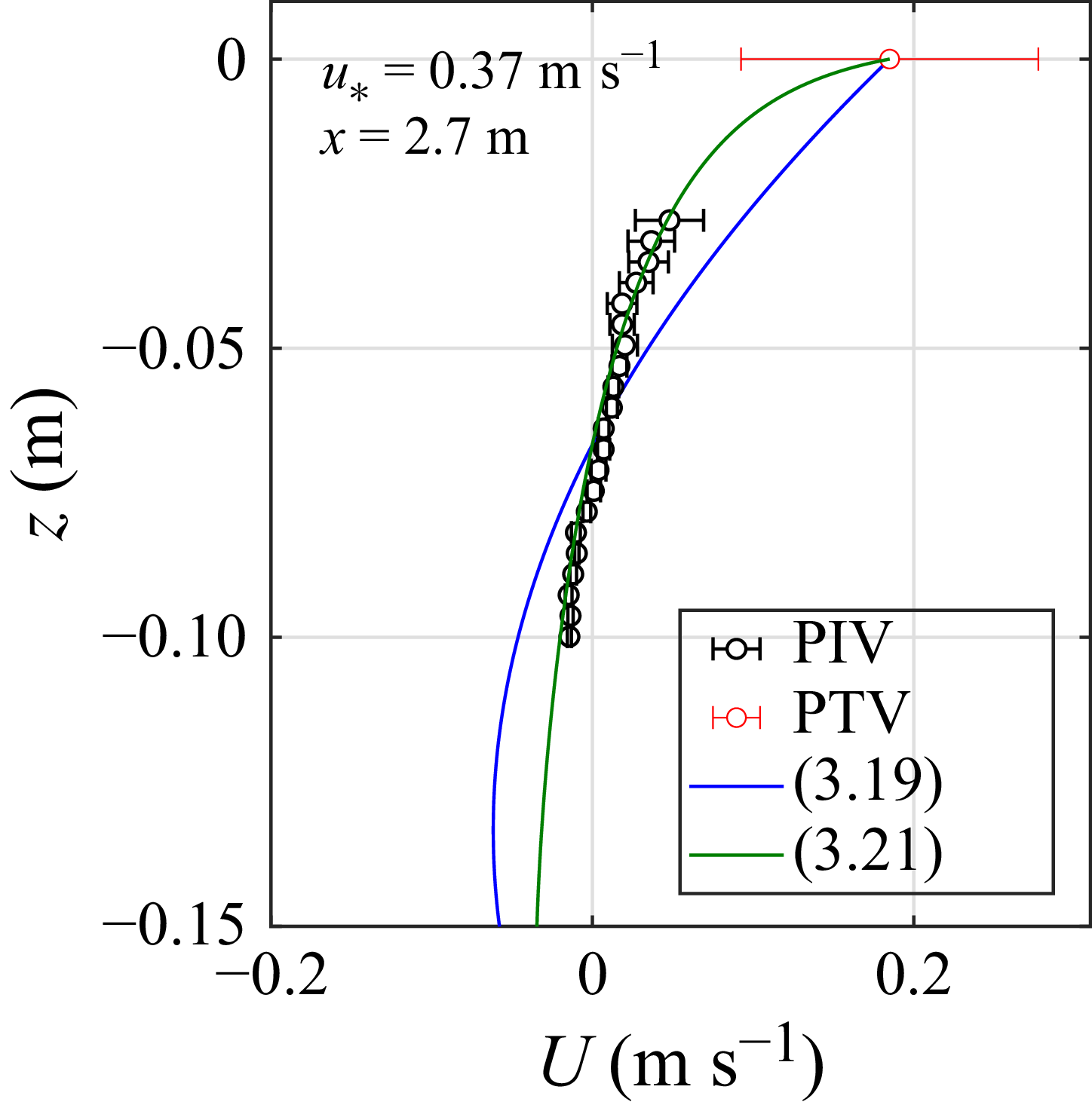


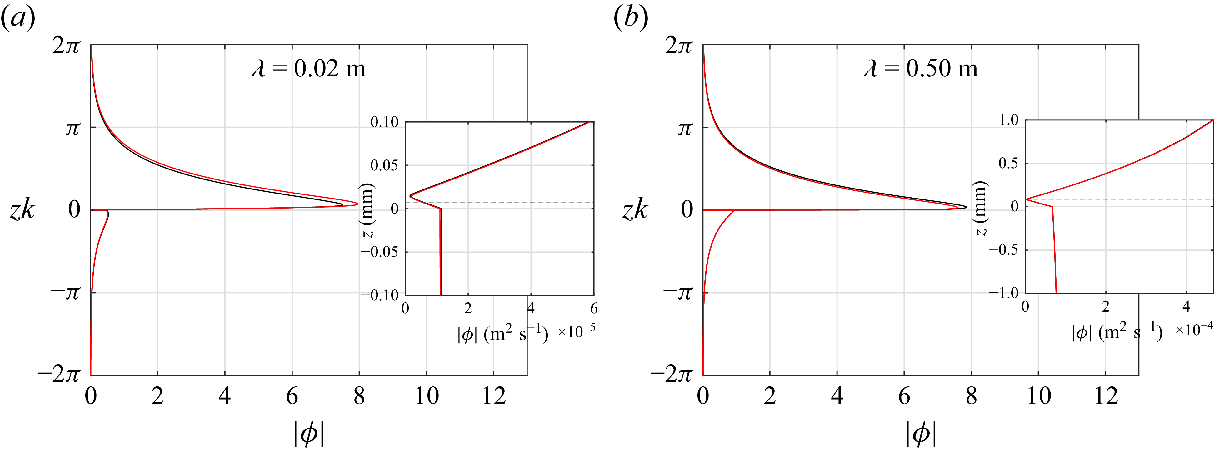


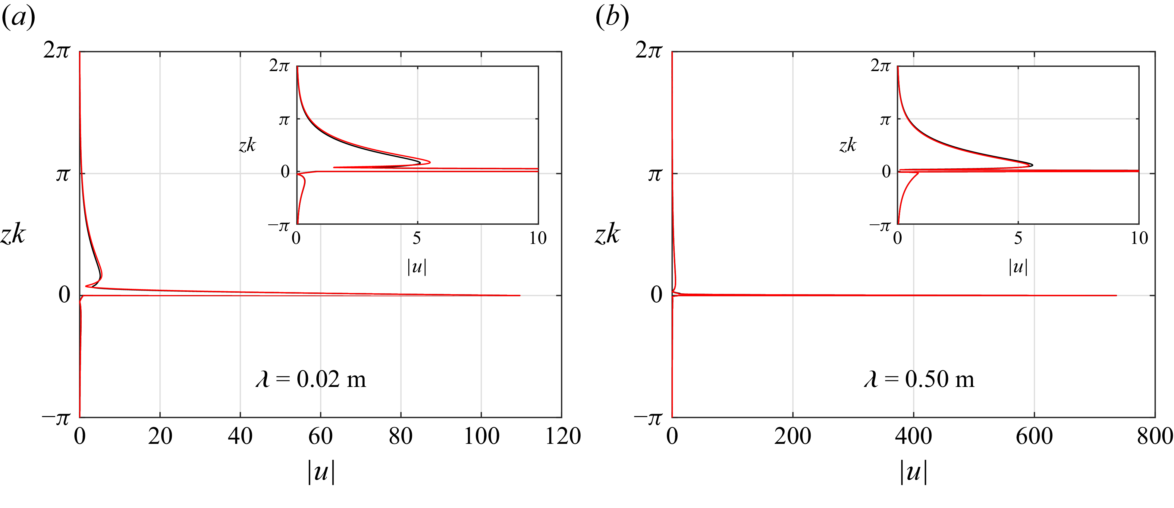


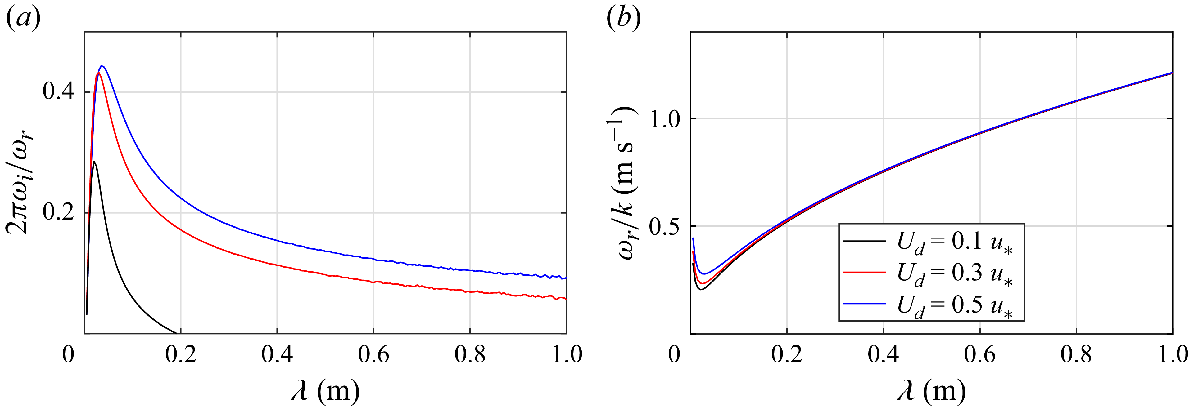


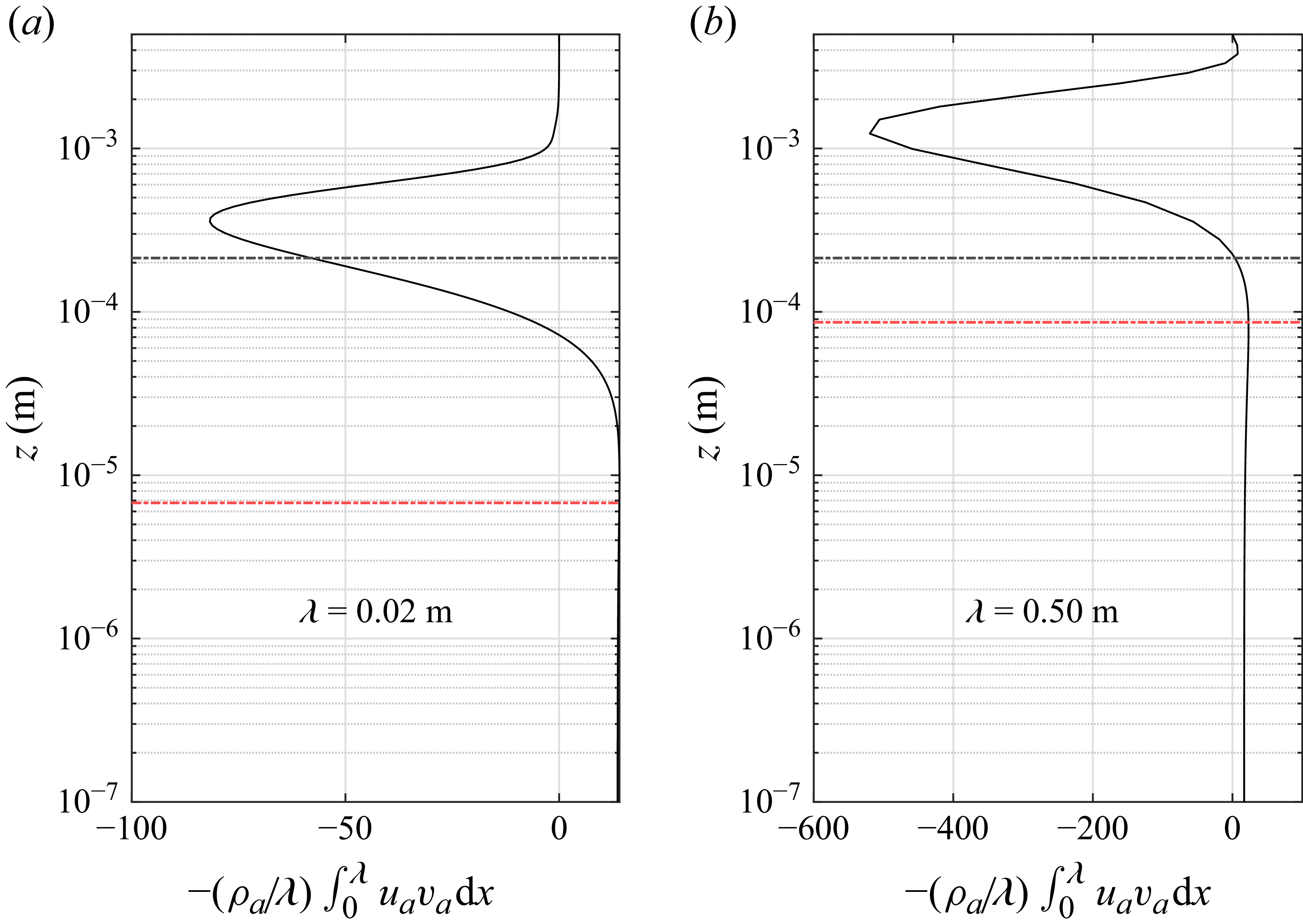


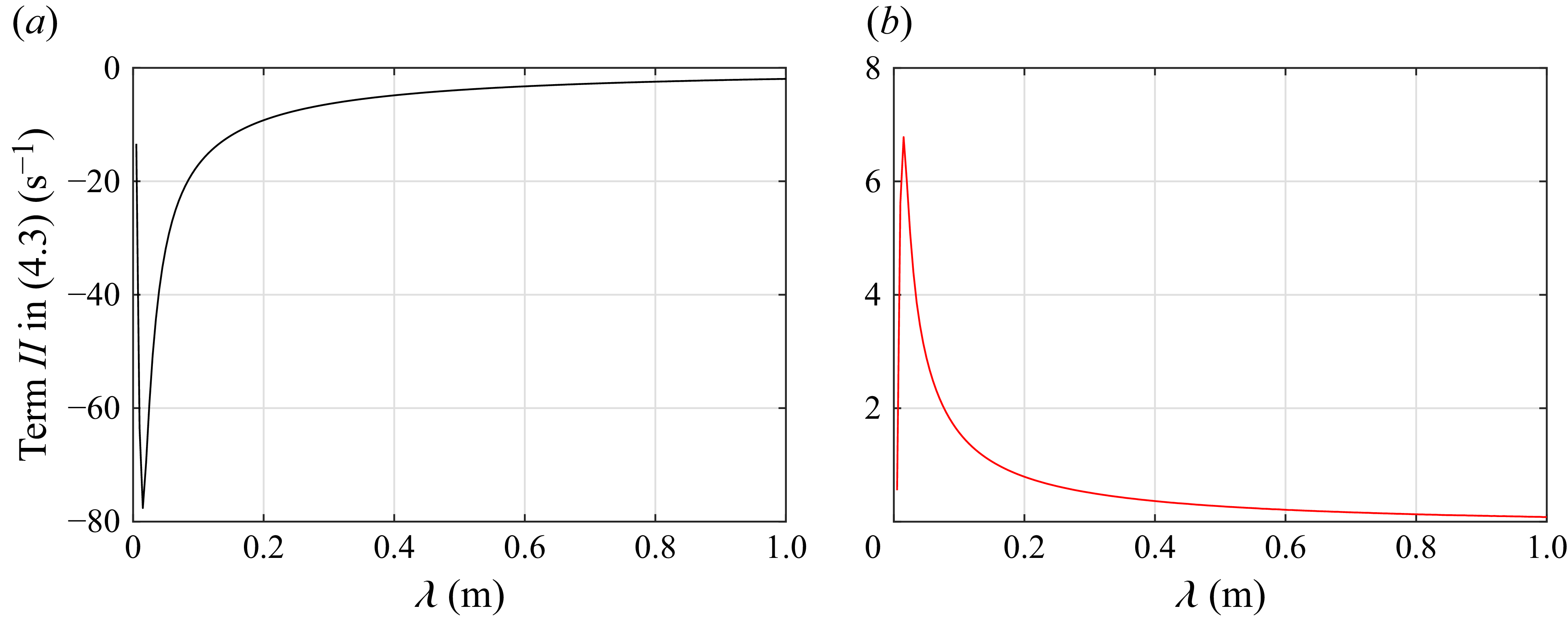


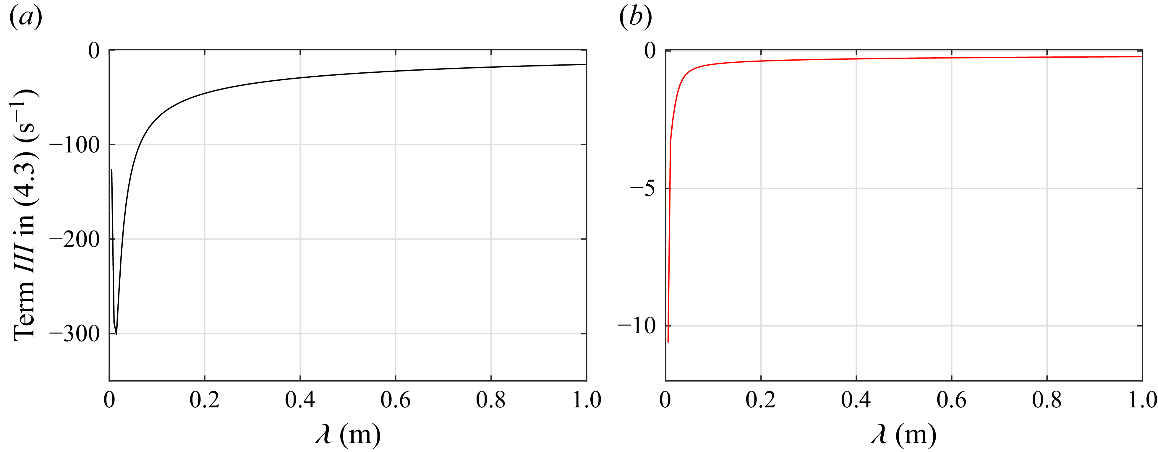


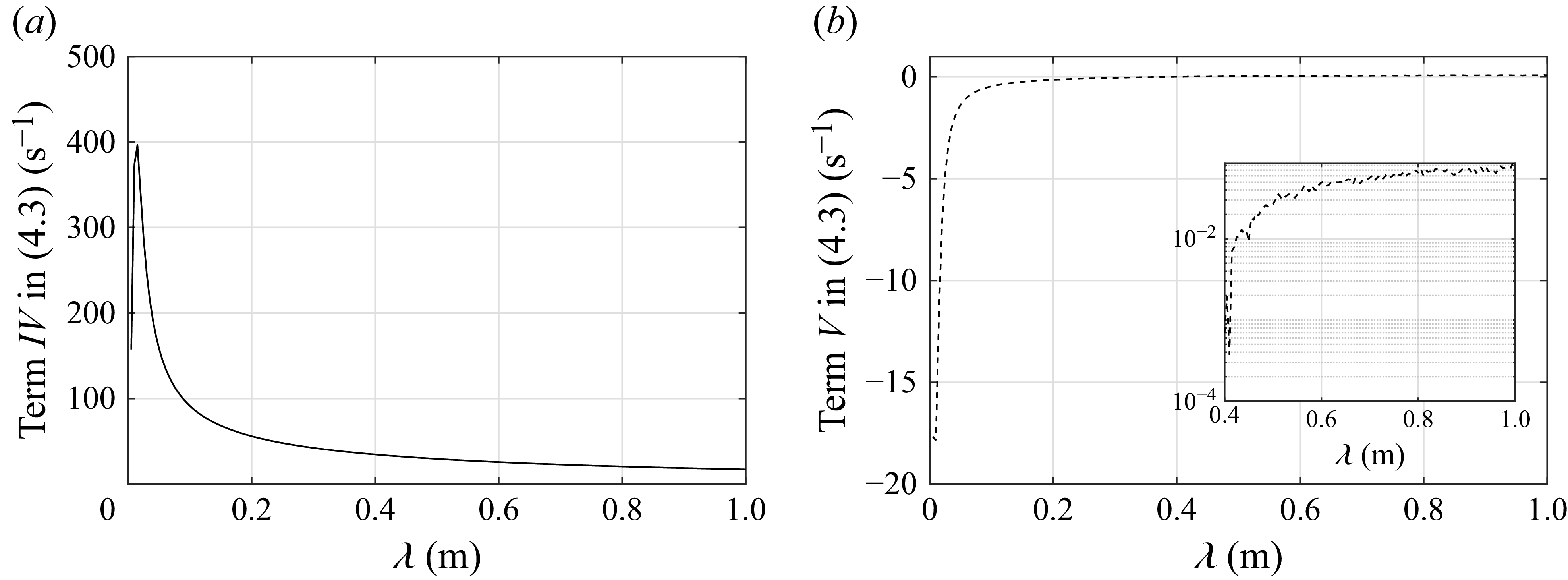


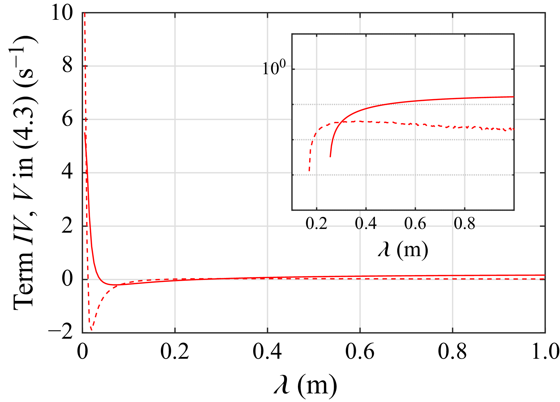


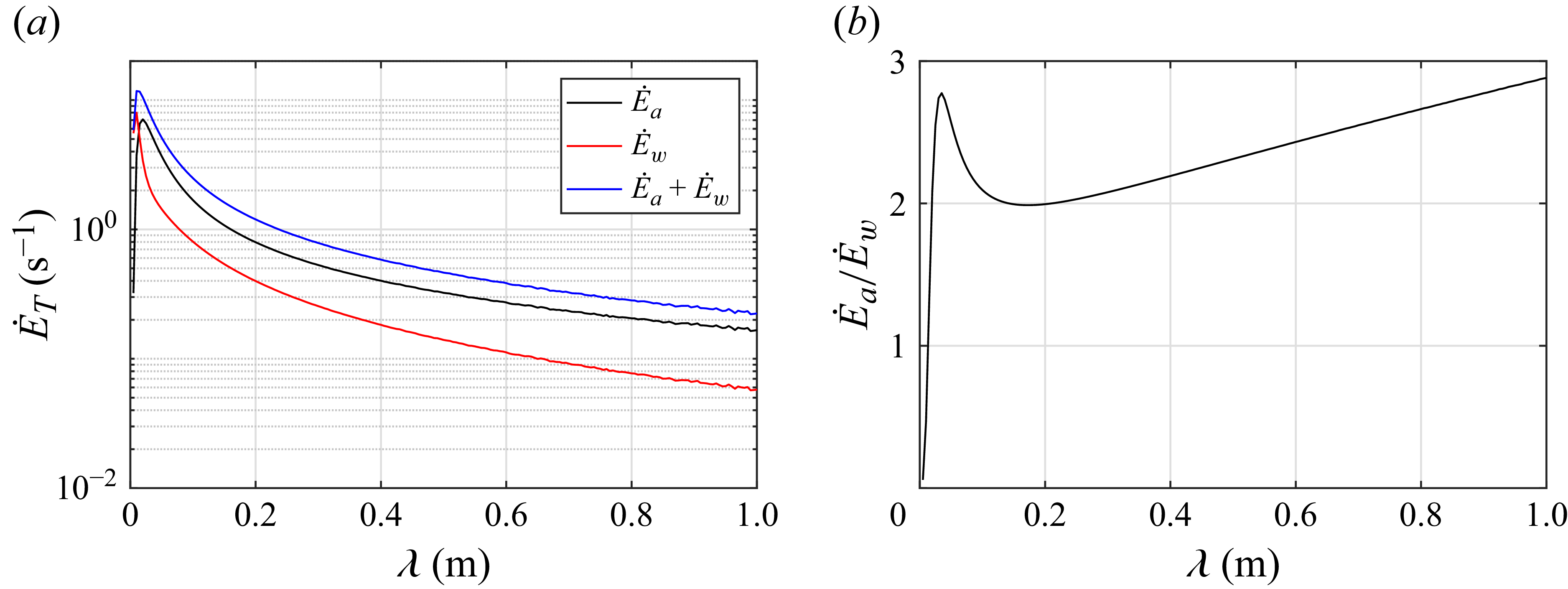


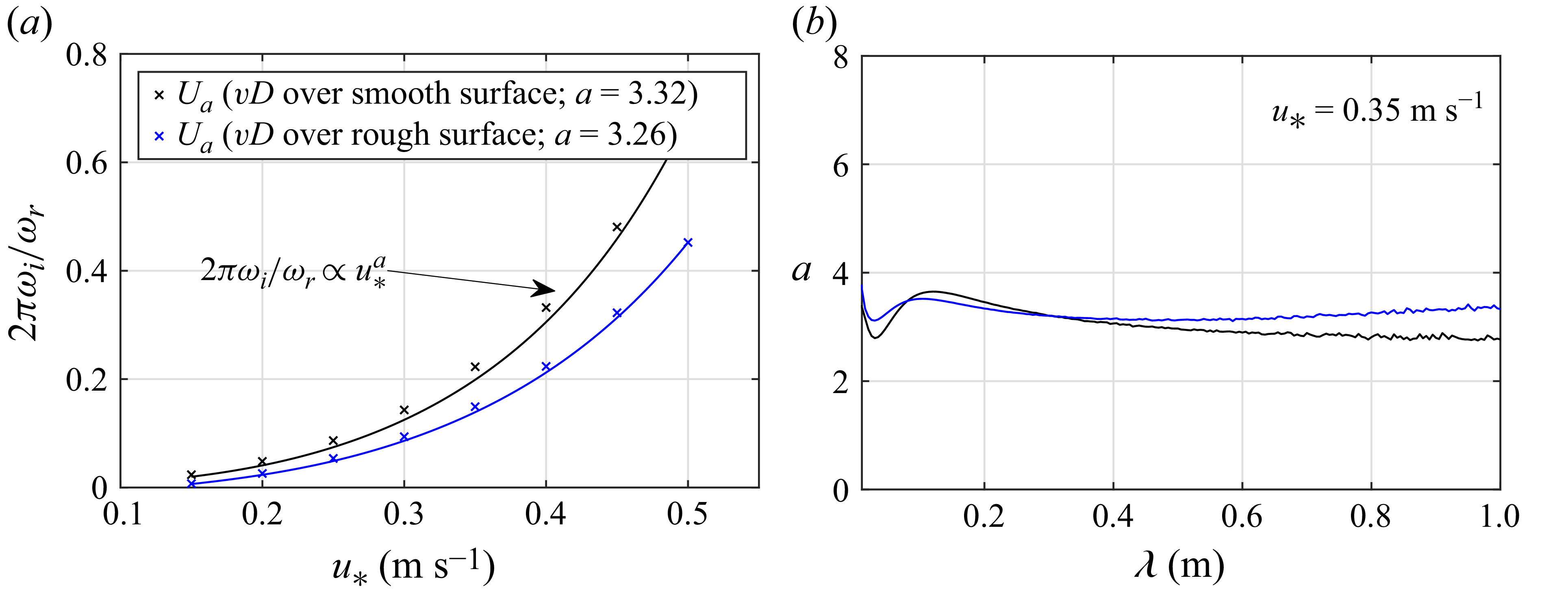


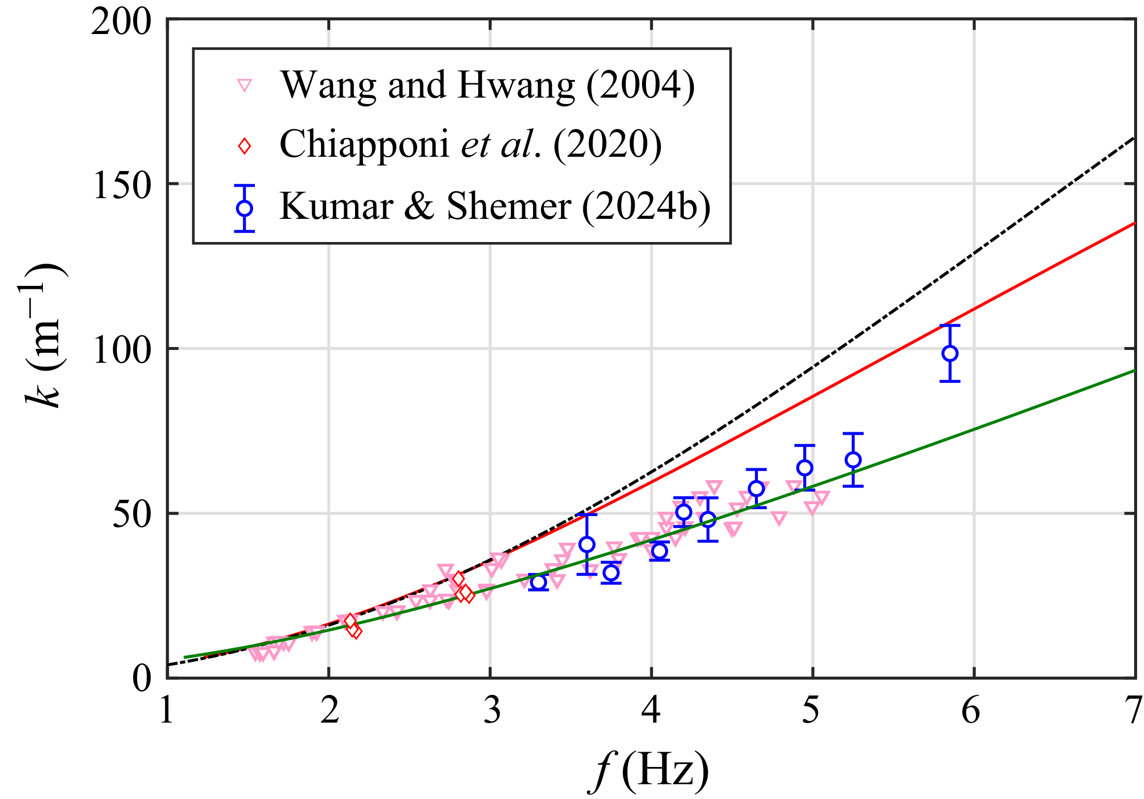


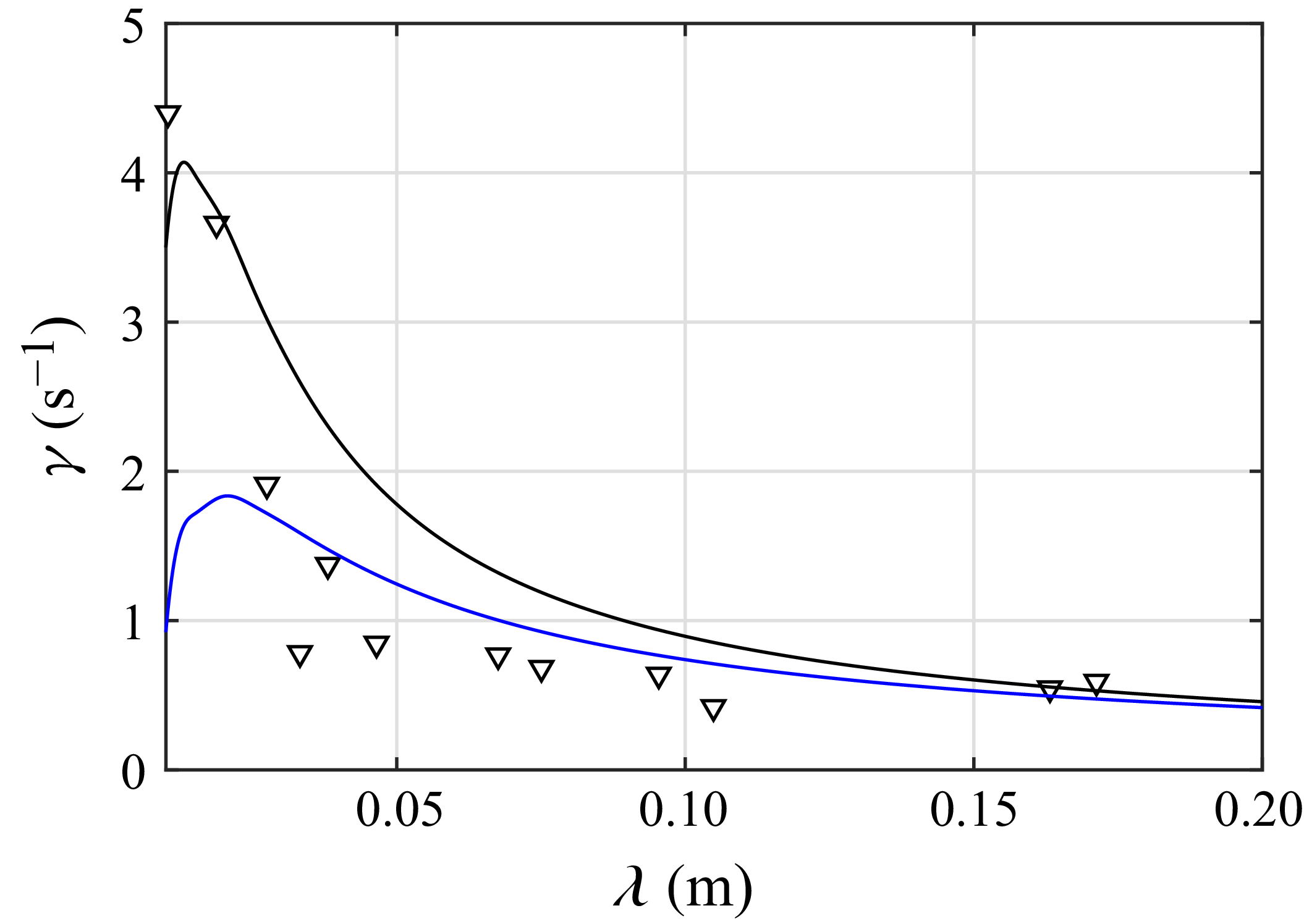


 Open access