2.1 Optical configuration

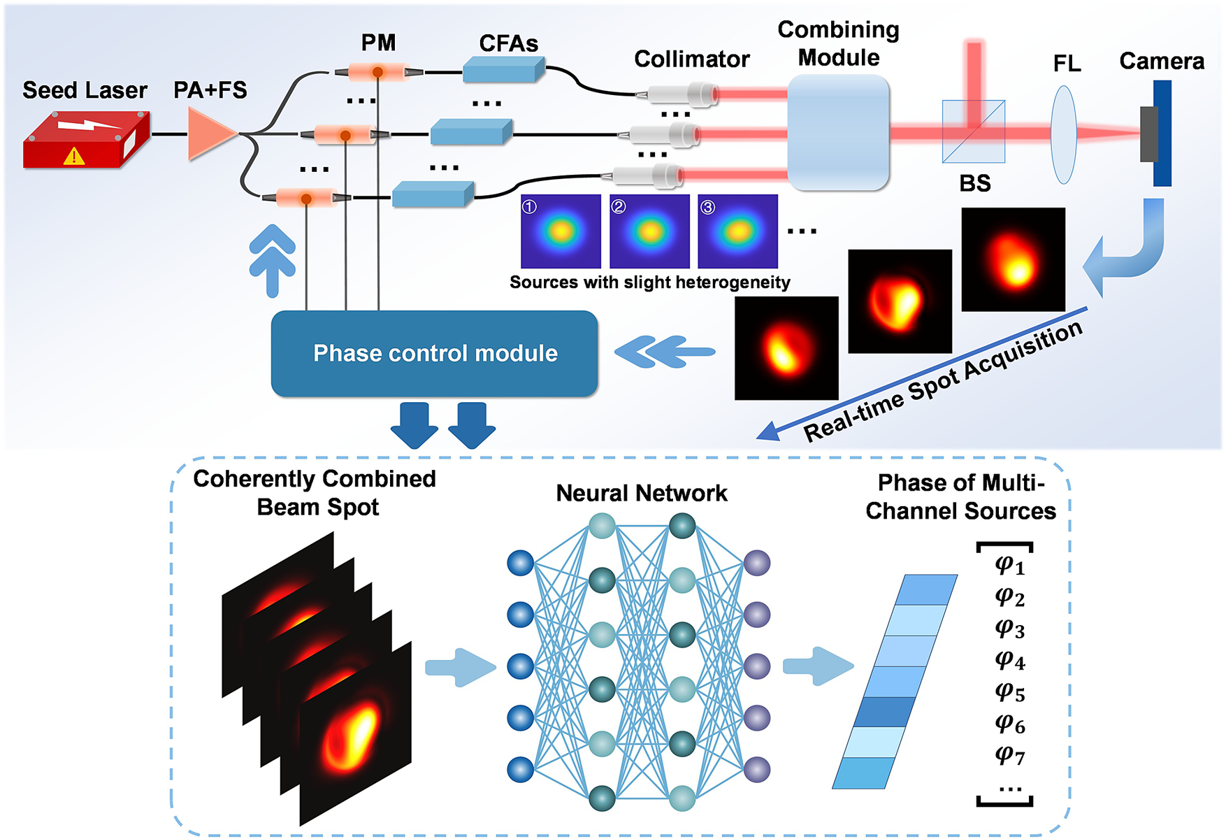
The optical configuration enabling neural-network-based phase locking for filled-aperture CBC is illustrated in Figure 1. A seed laser comprises a single-frequency fiber laser and a high-frequency phase modulator to spectrally broaden the output and suppress stimulated Brillouin scattering (SBS). The beam passes through a pre-amplifier before being split into multiple channels via a beam splitter, serving as seeds for individual channels. Then, each channel incorporates a low-frequency phase modulator and cascaded amplifiers, followed by a collimator. The combining module encompasses any filled-aperture coherent combining scheme, such as diffractive optical elements^[ Reference Redmond, Ripin, Yu, Augst, Fan, Thielen, Rothenberg and Goodno^35], photonic lanterns^[ Reference Montoya, Aleshire, Hwang, Fontaine, Velázquez-Benítez, Martz, Fan and Ripin^36] or polarizing beam splitters^[ Reference Uberna, Bratcher and Tiemann^37]. A fraction of the combined output is diverted to a simulated camera via a beam splitter and a lens. The combined laser spot pattern is then processed by the phase control module, which outputs the control voltages for phase modulators. This module hosts a neural network trained to decode phase states from the spot pattern. The critical challenge lies in establishing a one-to-one mapping between the spot pattern and multi-source phases and overcoming phase ambiguity. Our approach utilizes source mode nonuniformity to break ambiguity constraints, followed by neural-network-based decoupling of deep features within the pattern. Detailed explanation follows in subsequent sections.

Figure 1

The optical configuration enabling neural-network-based phase locking for filled-aperture CBC. PA, pre-amplifier; FS, fiber splitter; PM, phase modulator; CFA, cascaded fiber amplifiers; BS, beam splitter; FL, focus lens.

To provide sufficient data for the neural network, a large number of output intensity profiles and corresponding phase distributions need to be generated. Starting from the optical fields emitted by individual fibers, we simulate the field evolution of each source and finally compute the coherent combination to obtain the output beam profile. Given that multiple propagation processes are involved and the transverse size of the field may vary significantly at different planes, the Fresnel diffraction integral algorithm, which offers higher precision, is adopted here. The governing equation is as follows^[ Reference Hudson^38]:

(1) $$\begin{align}u\left(x,y\right)&=\frac{\exp (ikd)\cdot \exp \left[\frac{i k}{2d}\left({x}^2+{y}^2\right)\right]}{i\lambda d}\underset{-\infty }{\overset{+\infty }{\iint }}{u}_0^{\prime}\left({x}_0,{y}_0\right)\nonumber\\&\quad\cdot \exp \left[\frac{i k}{2d}\left({x_0}^2+{y_0}^2\right)\right] \nonumber\\&\quad \cdot\exp \left[-\frac{i k}{d}\left({x}_0x+{y}_0y\right)\right]\mathrm{d}{x}_0{\mathrm{d}y}_0,\end{align}$$

where $u(x,y)$ denotes the diffracted optical field at the observation plane, ${u}_0^{\prime}({x}_0,{y}_0)$ is the complex amplitude distribution at the source plane, $k$ is the wavenumber with $\lambda$ being the wavelength of the incident light and $d$ is the propagation distance between the source plane and the observation plane. The coordinates $({x}_0,{y}_0)$ and $(x,y)$ represent the transverse positions in the source and observation planes, respectively.

Direct evaluation of this equation is computationally intensive. Therefore, a secondary transformation has to be applied. By discretizing the integral term in Equation (1), the summation can be reformulated as matrix operations, allowing all terms to be evaluated simultaneously. This can significantly improve computational efficiency. The implementation is described in Ref. [Reference Gong, Li, Chen, Fang and Zhou39].

The effect of the lens on the optical field is represented by a quadratic phase factor:

(2) $$\begin{align}{u}_1^{\prime}\left({x}_1,{y}_1\right)=\exp \left(-i\frac{k}{2f}\left({x_1}^2+{y_1}^2\right)\right)\cdot {u}_1\left({x}_1,{y}_1\right),\end{align}$$

where $f$ is the focal length of the lens and $({x}_1,{y}_1)$ denote the transverse coordinates in the lens plane. The quadratic phase factor describes the modulation introduced by the lens, which enables focusing at the focal plane.

With the above equations, we are now equipped to simulate the final coherently combined field. Note that ${u}_0^{\prime}({x}_0,{y}_0)$ , the complex amplitude distribution at the source plane, represents the optical field of each source after phase modulation:

(3) $$\begin{align}{u}_{0j}^{\prime}\left({x}_0,{y}_0\right)=\exp \left(i{\varphi}_j\right)\cdot {u}_{0j}\left({x}_0,{y}_0\right),\end{align}$$

where the subscript $j$ is used to label different laser sources.

2.2 Nonuniformity among multiple fiber laser sources

To proceed, it is necessary to determine the field distribution of each laser source. As is well known, CBC typically requires polarization-maintaining, narrow-linewidth fiber lasers as the light sources^[ Reference Wang, Peng, Liu, Yang, Yu, Wang, Wang, Feng, Sun, Ma, Gao and Tang^40]. In theory, we desire these sources to have identical output power, linewidth, beam quality and polarization extinction ratio (PER) – in other words, to be uniform. However, in practice, especially when a large number of fiber laser sources are involved, it is virtually impossible to ensure complete consistency among all output characteristics, regardless of how carefully the system is managed. This leads to unavoidable nonuniformity among sources in CBC systems. This nonuniformity can manifest as differences in power, linewidth, mode distribution and PER. In this work, we focus particularly on modal nonuniformity. Due to the differences in fiber bending, fiber length, splicing conditions and other factors, the gain evolution in nominally identical fiber lasers can still vary^[ Reference Schermer and Cole^41], even if the differences are small. This phenomenon is especially common in large-mode-area fibers. Consequently, the modal power distribution and relative phase of the output beams differ across sources, leading to differences in their output intensity profiles^[ Reference Schermer and Cole^41].

For filled-aperture CBC, the output beams from all channels are spatially overlapped in both the near-field and far-field. This results in high beam quality and minimizes energy loss due to sidelobes^[ Reference Zhou, Tao, Feng, Zhang, Li, Xin, Peng, Lin, Wang, Yan and Jing^28]. However, such overlap introduces a significant issue. Consider an ideal scenario in which all lasers have identical power and Gaussian beam profiles, and their beam directions are perfectly aligned. Under such conditions, a given combined beam intensity profile could result from many different phase configurations, making it impossible to determine the exact relative phase of each source. This phase ambiguity assumes that all output beam profiles are identical, a condition that, as discussed above, is not realistic in practice. Based on this consideration, we take advantage of the modal nonuniformity, which ensures that even with the same set of relative phases, different sources produce distinct combined beam profiles. This effectively ‘labels’ each laser source with a unique modal feature. These distinct ‘labels’ manifest as identifiable differences in the combined beam intensity pattern, thus enabling a reliable mapping from the output beam to the underlying phase configuration.

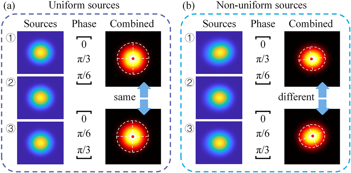
To illustrate this concept more intuitively, we consider a simplified case involving three fiber laser sources. As shown in Figure 2(a), suppose all three sources emit Gaussian beams. Phase shifts of 0, π/3 and π/6 are applied, with one beam serving as a reference (phase = 0). Swapping the phases of the other two beams results in the same combined intensity profile. This is a clear example of phase ambiguity. In contrast, when higher-order modes are introduced into the source fields, making the beam profiles non-identical (Figure 2(b)), the combined beam intensity patterns become distinguishable when the applied phase shifts are swapped. The phase ambiguity is resolved by modal nonuniformity.

Figure 2

CBC beam intensity distribution with uniform sources and nonuniform sources. (The red dots indicate the centroid positions of the combined beam.)

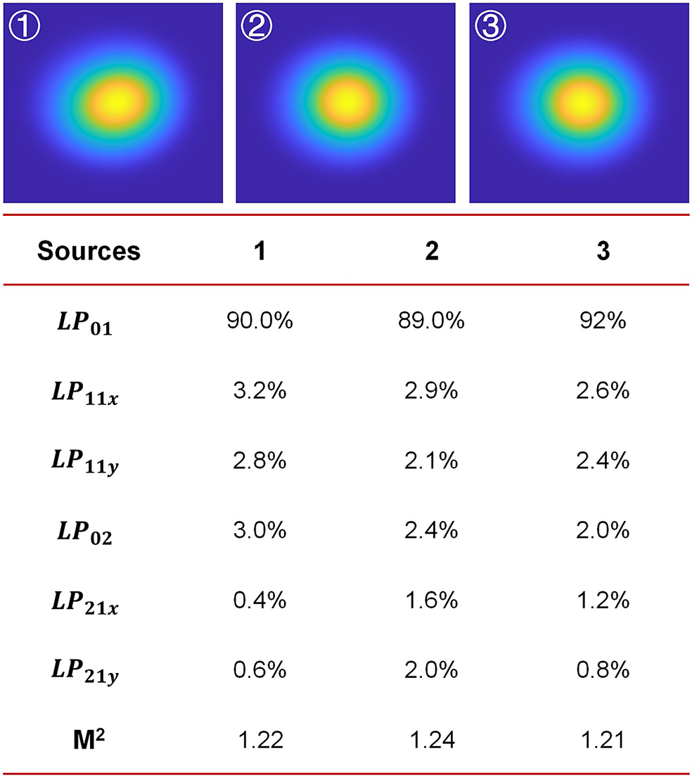
By adjusting the proportions of higher-order mode content, slight variations in the output beam profiles of the fibers can be introduced. An example of the mode power distribution for three sources is shown in Figure 3. The fiber parameters are set as 25/400 μm with a numerical aperture (NA) of 0.065. For such fibers, the stable guided mode is LP₀₁. The LP₀₁ mode accounts for approximately 90% of the total power, while all other modes together constitute about 10%. The beam quality factor (M ²) of each source is calculated to be close to 1.2.

Figure 3

The mode power distribution and beam quality for nonuniform sources.

Once the output fields of all sources are obtained, the dataset required for training the network can be efficiently generated using a computer. By randomly assigning phases to each source, the intensity distribution of each beam can be calculated using Equation (1). The intensity distribution of the combined beam can be given by the following:

(4) $$\begin{align}I\left({x}_{\mathrm{fp}},{y}_{\mathrm{fp}}\right)={\left|\sum \limits_{j=1}^n{u}_{\mathrm{fp}j}\left({x}_{\mathrm{fp}},{y}_{\mathrm{fp}}\right)\right|}^2,\end{align}$$

where $({x}_{\text{fp}},{y}_{\text{fp}})$ are the transverse coordinates of the focal plane, ${u}_{\text{fp}j}({x}_{\text{fp}},{y}_{\text{fp}})$ represents the focal-plane field contribution from different laser sources, the index $j$ labels each individual source and $n$ is the total number of laser sources. It is important to note that practical CBC requires beam alignment. Accordingly, our simulation also incorporates beam alignment considerations. For simplicity, this is modeled as centroid alignment. The centroid of each source’s output field is calculated using the following expression:

(5) $$\begin{align}\overline{x_0}&=\frac{\int_{-\infty}^{+\infty }{\int}_{-\infty}^{+\infty } xI\left(x,y\right)\mathrm{d}x\mathrm{d}y}{\int_{-\infty}^{+\infty }{\int}_{-\infty}^{+\infty }I\left(x,y\right)\mathrm{d}x\mathrm{d}y},\nonumber\\\overline{y_0}&=\frac{\int_{-\infty}^{+\infty }{\int}_{-\infty}^{+\infty } yI\left(x,y\right)\mathrm{d}x\mathrm{d}y}{\int_{-\infty}^{+\infty }{\int}_{-\infty}^{+\infty }I\left(x,y\right)\mathrm{d}x\mathrm{d}y},\end{align}$$

where $I$ is the intensity distribution of the optical field on this plane.

Due to the modal nonuniformity among the sources, slight deviations in the beam centroid positions naturally exist. After aligning the centroids of all output fields on the focal plane, the intensity distribution of the combined beam can be calculated. This intensity profile, after normalization, serves as the input to the neural network. Normalization is applied not only to meet the requirements of neural network training, but also to account for the automatic exposure behavior commonly present in camera-based beam acquisition systems. For the network output, prior studies have shown that representing each phase using its sine and cosine components improves prediction accuracy and avoids the discontinuity inherent in phase periodicity^[ Reference Zhou, Tao, Feng, Zhang, Li, Xin, Peng, Lin, Wang, Yan and Jing^28]. Therefore, we adopt a 1×2 $n$ vector as the network output, where $n$ is the number of beams.

2.3 Neural network construction

Although the source nonuniformity can help mitigate the phase ambiguity problem, the mapping between the combined speckle and the multi-source phase distribution is generally very hard to resolve, especially as the number of sources increases. Therefore, we leverage the strong learning capability of neural networks to model this complex relationship.

From a conceptual perspective, a neural network can be viewed as a function approximator that learns the relationship between an input (the measured speckle intensity distribution) and an output (the corresponding multi-source phase distribution) directly from examples. Unlike conventional phase estimation or optimization-based approaches, this strategy does not require iterative calculations or detailed physical inversion models. Instead, the network infers the phase information through a single forward pass once training is completed, which significantly reduces computational complexity and is particularly suitable for multi-channel coherent beam combining systems. As the first choice, the Visual Geometry Group (VGG) neural network is adopted due to its implementation simplicity, sufficient depth and extensive validation in prior studies^[ Reference Hou, An, Chang, Ma, Li, Zhi, Huang, Su, Wu, Ma and Zhou^22, Reference Hou, An, Chang, Ma, Li, Huang, Zhi, Wu, Su, Ma and Zhou^23, Reference Zhou, Tao, Feng, Zhang, Li, Xin, Peng, Lin, Wang, Yan and Jing^28]. Given that the objective is to demonstrate the feasibility and robustness of neural-network-based phase estimation rather than to benchmark different network designs, the VGG neural network provides a suitable balance between model capacity and implementation transparency. The VGG network used in this work consists of two main components: a feature extraction module and a regression prediction module. The input to the network is a single-channel speckle image generated from filled-aperture CBC. The image is then passed through seven cascaded convolution blocks for feature extraction. Each block contains multiple 3×3 convolutional layers with rectified linear unit (ReLU) activation and the same padding, followed by a 2×2 max-pooling layer with a stride of 2 for spatial down-sampling. The number of feature channels increases from 64 in the first block to 512 in the last block, enabling hierarchical extraction of spatial features from the speckle patterns. The regression prediction module consists of three fully connected layers with 4096 neurons each, both using ReLU activation. Dropout with a rate of 0.5 is applied after each fully connected layer to reduce overfitting. The output layer contains 14 neurons with a tanh activation function, constraining the predicted values to the range [−Reference Xiong, Ma, Wu, Su, Zhou and Si1,1]. The outputs are reshaped into a 14×1 vector corresponding to the phase-related parameters of the individual light sources. In total, the VGG network employed here comprises 19 convolution layers and 3 fully connected layers, enabling an end-to-end mapping from speckle images to target phase vectors via progressive spatial compression.

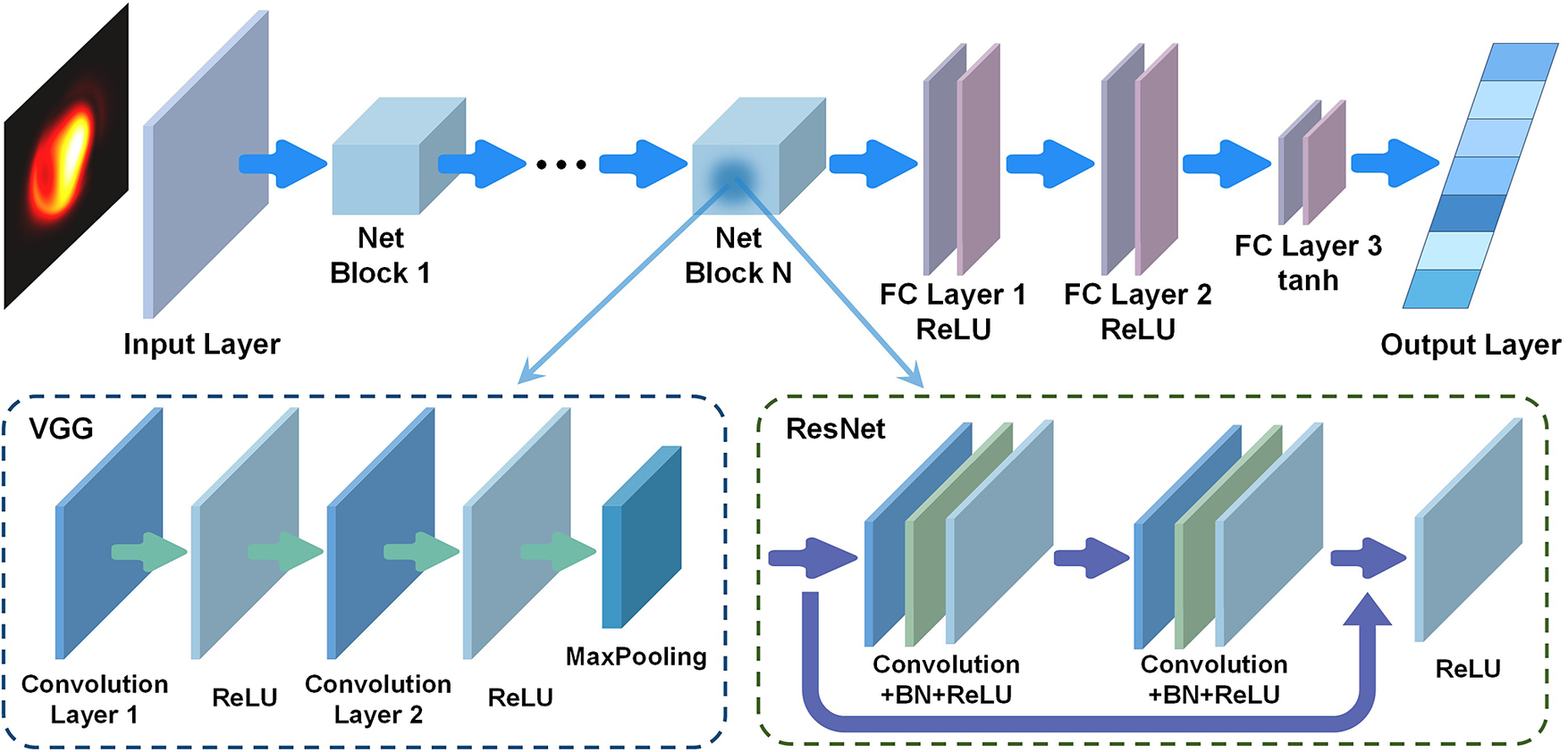
In addition, the ResNet neural network, which has demonstrated outstanding performance in image recognition tasks^[ Reference Haque, Lim and Kang^42, Reference Liu, Jin, Li, Wu, Ma, Su, Leng and Zhou^43], is also employed for phase reconstruction. The ResNet architecture is a deep convolutional neural network that introduces residual connections to facilitate the training of deeper models. Instead of learning a direct mapping between the input and output of a convolutional block, ResNet learns a residual mapping, where the input feature map is added to the output of the convolutional layers. This design helps alleviate gradient vanishing and improves training stability. Each residual block typically consists of convolutional layers followed by batch normalization (BN) and nonlinear activation, with a shortcut connection that bypasses these layers. The ResNet network used in this work differs from the VGG network primarily in the construction of the network blocks, as illustrated in Figure 4. Since the ResNet blocks here do not include max-pooling operations, down-sampling is applied between blocks. Before entering the fully connected layers, average pooling is performed to reduce the spatial dimensions. Moreover, we also investigate an MLP model for phase retrieval. This model has a much simpler structure. After flattening the speckle image into a one-dimensional vector, only two fully connected layers are used to compress it to the size of the target phase vector. The hidden-layer size in the MLP is 6.

Figure 4

The structure of the VGG and ResNet neural networks employed in this work. BN, batch normalization.

3.1 25-channel filled-aperture CBC utilizing the VGG network

For the 25-channel CBC task, 35,000 data pairs are generated using the method described above. Each fiber laser is collimated with a lens of 75 mm focal length. For systems with fewer channels, fewer sampling points and shorter focal lengths are sufficient. This is because, with a larger number of beams, the nonuniform characteristics among sources become more complex and require higher spatial resolution to distinguish. Increasing the focal length and sampling density helps improve the accuracy of phase reconstruction by the network.

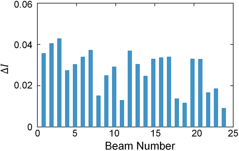
To quantitatively characterize the differences in source field distribution, the following definition is introduced:

(6) $$\begin{align}\begin{array}{c}\Delta {I}_i=\frac{\int_{-\infty}^{+\infty }{\int}_{-\infty}^{+\infty}\left|{I}_i\left(x,y\right)-{I}_1\left(x,y\right)\right|\mathrm{d}x\mathrm{d}y}{\int_{-\infty}^{+\infty }{\int}_{-\infty}^{+\infty }{I}_1\left(x,y\right)\mathrm{d}x\mathrm{d}y}.\end{array}\end{align}$$

Here, $i$ denotes the index of the light source and ${I}_i$ represents the normalized optical field of the $i$ th source. This quantity is used to evaluate the nonuniformity of the laser sources employed in the simulations. The values of $\Delta I$ of fiber lasers with identical configurations are measured and are generally no greater than 0.08. The distribution of $\Delta I$ for the light sources in the 25-channel simulations is shown in Figure 5. The values of $\Delta I$ fall within the range observed in the experimental measurements.

Figure 5

Distribution of ΔI for the light sources in the 25-channel simulations.

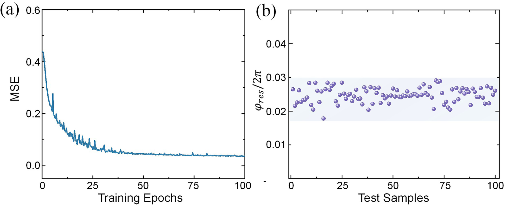
The network is trained in a supervised manner using the mean squared error (MSE) as the loss function. The VGG network is trained using a batch size of 128, with stochastic gradient descent with momentum as the optimizer. Model optimization is performed using the Adam optimizer with the learning rate of 0.003. The momentum factor is set to be 0.5, and the number of training epochs to be 100. Among the 35,000 data pairs, 30,000 are used for training, 3500 for validation and 1500 for testing. The loss curve is shown in Figure 6(a). Within the first 25 epochs, the loss drops rapidly below 0.10, and further decreases to 0.038 by the end of training. This indicates that the mapping between the speckle pattern and the multi-source phase distribution is successfully learned. Figure 6(b) shows the phase residuals of 100 prediction samples, with a mean value of λ/39. These results demonstrate that the proposed method achieves high accuracy and enables single-step phase locking.

Figure 6

Reconstruction results of the VGG network: (a) the loss curve for data pairs and (b) the phase residuals of 100 prediction samples.

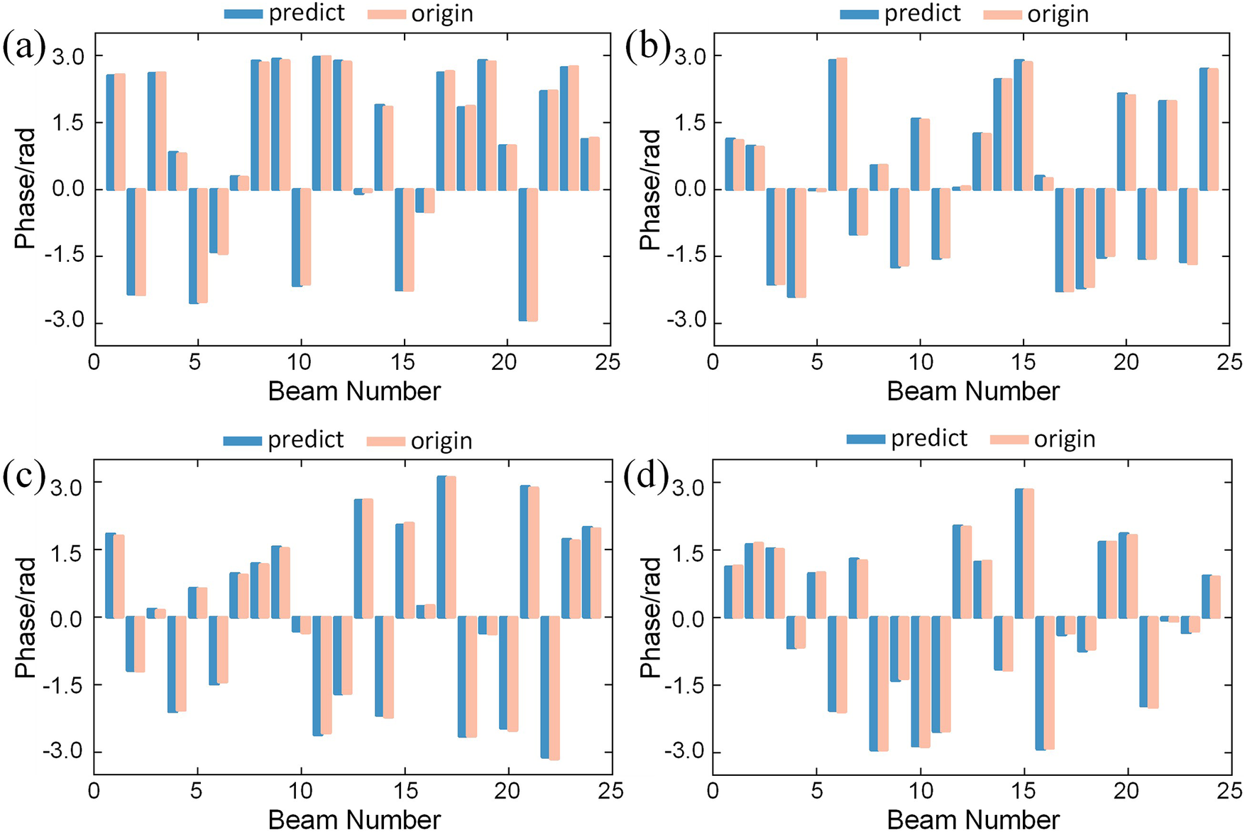
To illustrate the accuracy of our method, four test samples are selected. The predicted phases are obtained and compared with the original phase, as shown in Figure 7. It is worth noting that the neural network performs single-step prediction. In the selected samples, the predicted phases of the 24 channels (excluding the reference channel) show high consistency with the original values.

Figure 7

The predicted phases and original phase for four test samples after single-step prediction.

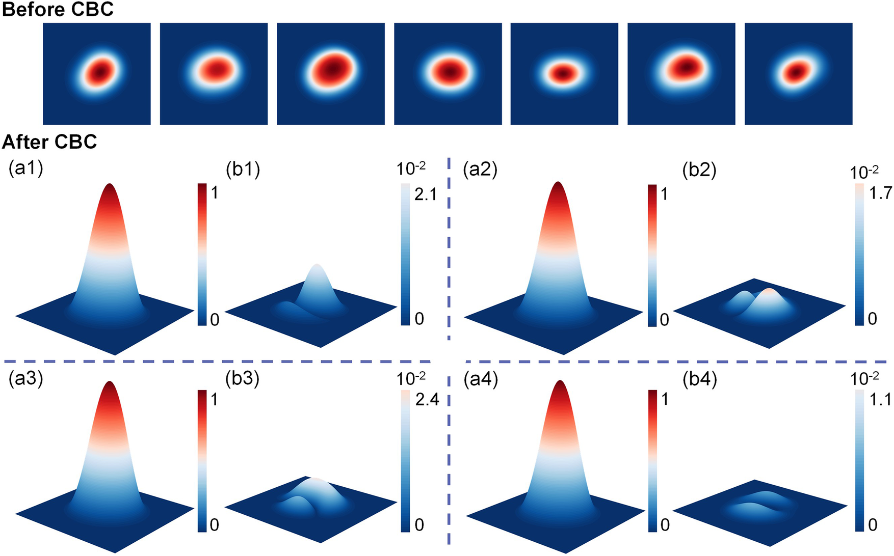
The difference in the combined beam intensity distribution before and after phase locking is shown in Figure 8. Before phase locking, due to the randomness of the phases, the beam profiles exhibit significant variations. After phase locking, the normalized intensity distribution of the beam is shown in Figures 8(a1)–(a4). There is no noticeable difference in the beam intensity distribution. Figures 8(b1)–(b4) present the difference between the ideal normalized combined beam intensity, which corresponds to zero phase difference across all sources, and the intensity distribution obtained using our phase locking method. The maximum deviation remains of the order of 10^–2. This indicates that the phase recovered by the neural network exhibits not only high accuracy but also strong stability.

Figure 8

The intensity distribution before and after the neural network phase locking. (a1)–(a4) Normalized intensity distribution after phase locking. (b1)–(b4) The difference from the ideal intensity distribution.

Figure 9

(a) Evolution of the loss functions during training. (b) Phase error after prediction for the VGG, ResNet and MLP networks.

For CBC with a larger number of channels, our method remains applicable. A simulation is conducted for 49-channel filled-aperture CBC. As previously analyzed, source nonuniformity is essential for enabling phase locking via neural networks. With more channels, the distinctive features of individual sources become more susceptible to being overwhelmed by noise. This imposes higher demands on the network’s ability to extract such features. Therefore, the number of training samples needs to be increased, and network parameters have been further optimized. 80,000 data pairs are used, namely 70,000 for training, 5000 for validation and 5000 for testing. The learning rate is decreased to 0.001 and the number of epochs is increased to 500. The phase residual reaches λ/24, which is acceptable for practical use, and the phase locking is still achieved in a single step.

3.2 Transferring to other networks

Our proposed method also exhibits strong adaptability to different neural network architectures, allowing targeted network design based on the quality of the training data. To illustrate this, we perform nine-channel filled-aperture CBC, which enables faster training. A relatively small dataset of 10,000 pattern–phase pairs is sufficient to achieve phase recovery. Among them, 8000 pairs are used as the training set, 1000 as the validation set and 1000 as the test set. We evaluate the recovery performance using three types of neural networks: the VGG, ResNet and MLP. The VGG network uses the same structure and parameters as in the 25-channel CBC case. The ResNet network, widely recognized for its effectiveness in image recognition tasks in computer vision, has been introduced in detail above. For the specific case of nine-channel CBC, we adopt four residual blocks, each consisting of two convolutional layers with 3×3 kernels. Compared to these convolutional networks, the MLP network is significantly simpler. The three networks have parameter scales of 248.38, 20.23 and 68.09 MB, respectively.

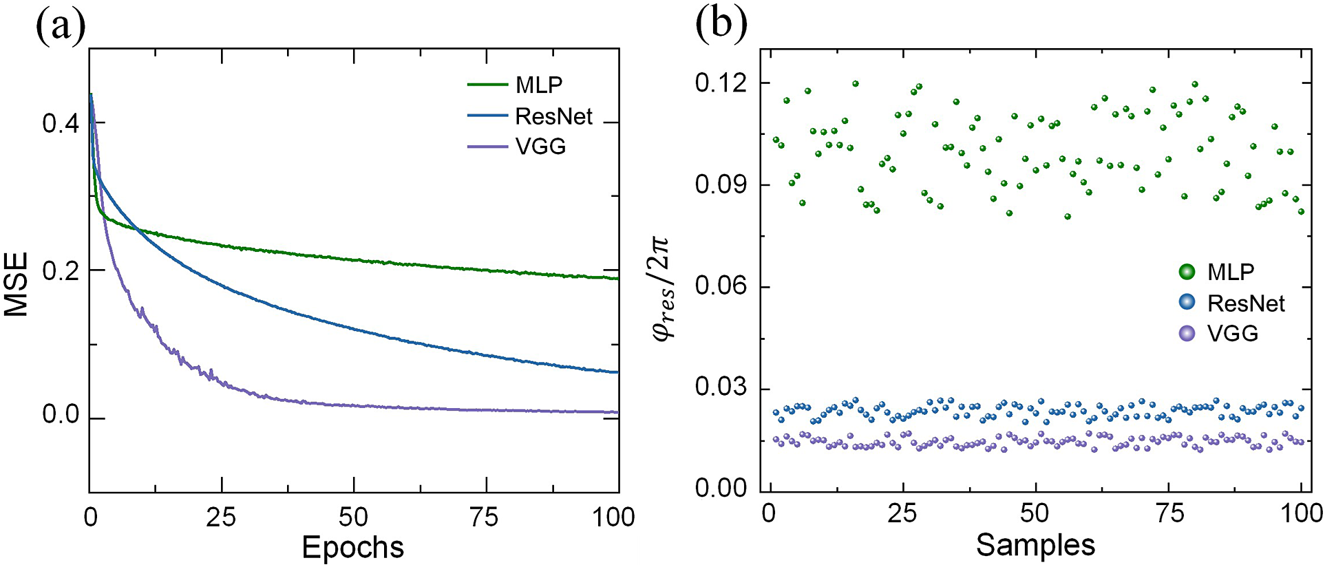
Figure 9 shows the evolution of the loss functions during training and the phase error after prediction for these three networks. Using the adopted VGG-based network, the training loss decreases below 0.10 within the first 25 epochs and further converges to 0.008 in subsequent epochs, corresponding to a mean phase estimation error of approximately λ/68. For reference, the ResNet network yields a final mean phase estimation error of approximately λ/38. Due to the simple structure and limited ability to extract deep features from the input images, the MLP network performs poorly. It maintains a high loss throughout training, with a final mean phase error of λ/10 and significant fluctuations, making it unsuitable for practical coherent beam combining applications. It should be noted that the goal of this comparison is not to benchmark different neural network architectures, but rather to validate the effectiveness of learning-based phase estimation under nonuniformity conditions.

Figure 10

(a) Convergence process of the SPGD algorithm and (b) the neural network method.

Figure 11

(a) Combining efficiency after introducing dynamic noise (the inset shows the results over a shorter time span). (b) Noise intensity distribution before and after phase locking.

The results show that different convolutional neural network architectures can be applied to the proposed phase estimation framework. The VGG-based network exhibits stable convergence behavior, while the ResNet-based network shows different learning characteristics, potentially due to the use of residual connections, which may influence feature representation in regression tasks^[ Reference Wang, Li and Vasconcelos^44]. These observations indicate that the proposed method is not restricted to a specific network design and can be extended to alternative architectures with appropriate training and optimization.

3.3 Comparison with SPGD and dynamic phase-locking simulation

Compared with traditional common-path phase-locking methods, the neural network method enables one-step, rapid prediction and compensation of phase. We selected 10 different multi-source phase distributions and performed phase reconstruction using both the widely adopted SPGD algorithm and our proposed method. The average combining efficiency across each step can serve as an indicator of the convergence capability of two methods. The SPGD algorithm employed here uses combined efficiency as the loss function, defined in Ref. [Reference Zhou, Feng, Xie, Li, Zhang, Tao, Lin, Wang, Yan and Jing5]. As shown in Figure 10(a), the SPGD method requires approximately 400 epochs to converge, whereas our approach achieves convergence in a single step (Figure 10(b)). The comparison demonstrates a significant advantage in convergence speed.

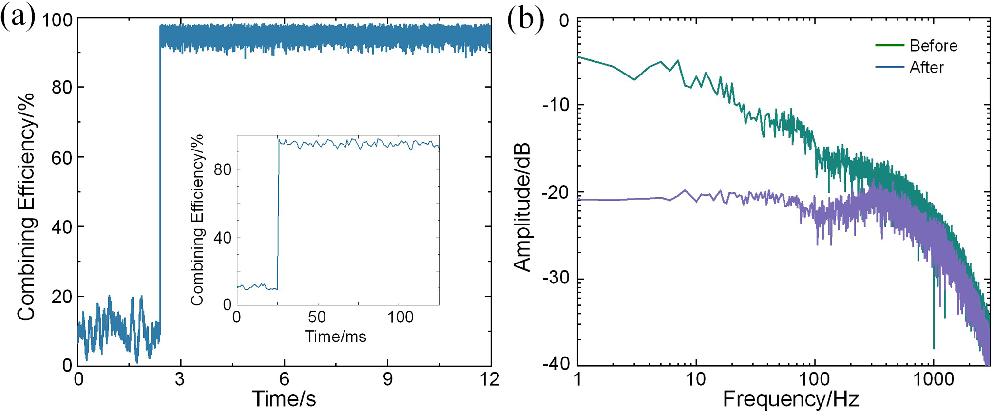
The above analysis is based on static phase reconstruction. However, in practical CBC, the phase is not constant but rather fluctuates dynamically, leading to time-varying combining efficiency. To evaluate the robustness of our approach under dynamic noise, simulation of dynamic phase locking using the VGG neural network is conducted. The simulation involves nine channels, and the size of the training dataset is the same as in the previous section. The phase-locking procedure involves two main steps: collecting the far-field beam spot and reconstructing the corresponding phase. The time required for one complete locking step is defined as the locking duration and determines the locking repetition rate. It is important to note that beam sampling occurs at the beginning of a locking step, while the reconstructed phase is applied to each channel at the end. This introduces a delay, meaning the reconstructed phase, which is based on the earlier sampled pattern, may differ from the actual noise phase when applied. This may lead to reduced accuracy under dynamic conditions compared to static ones.

Dynamic phase noise is modeled using bandwidth-limited white noise^[ Reference Augst, Fan and Sanchez^45], reflecting the dominance of low-frequency noise in practical systems. The phase noise amplitude is set to λ/20^[ Reference Jones, Stacey and Scott^46], and the locking repetition rate is 1 kHz. Figure 11(a) shows the combined efficiency before and after locking. Without phase locking, the efficiency fluctuates at a low level due to both static and dynamic phase errors. Once phase locking is initiated, the low-frequency phase noise below the locking rate is largely compensated, leading to a significant improvement in efficiency, with an average around 97% and notably reduced fluctuations. The residual fluctuations are caused by high-frequency noise, which is more difficult to compensate. Figure 11(b) displays the noise power spectral density before and after locking. It clearly shows that phase noise below 1 kHz is effectively suppressed, indicating a 1 kHz locking bandwidth. In practice, higher bandwidths can be achieved by adopting faster phase control devices.