


1. Introduction
Fluid flow and solute dispersion through slender annular conduits is fundamental to various biological and engineered systems. Examples include microfluidic devices (Zhao & Bau Reference Zhao and Bau2007; Hardoüin et al. Reference Hardoüin, Laurent, Lopez-Leon, Ignés-Mullol and Sagués2020), catheter flows (Dash, Jayaraman & Mehta Reference Dash, Jayaraman and Mehta1996; Sarkar & Jayaraman Reference Sarkar and Jayaraman2001), transport in xylem and phloem (Nakad et al. Reference Nakad, Witelski, Domec, Sevanto and Katul2021), flow in bones (Cowin & Cardoso Reference Cowin and Cardoso2015), the subarachnoid space in the brain, spinal chord and optic nerve sheath (Loth, Yardimci & Alperin Reference Loth, Yardimci and Alperin2001; Sánchez et al. Reference Sánchez, Martinez-Bazan, Gutiérrez-Montes, Criado-Hidalgo, Pawlak, Bradley, Haughton and Lasheras2018; Salerno, Cardillo & Camporeale Reference Salerno, Cardillo and Camporeale2020; Rossinelli et al. Reference Rossinelli, Fourestey, Killer, Neutzner, Iaccarino, Remonda and Berberat2024) and perivascular spaces (PVSs) in the brain (Iliff et al. Reference Iliff2012; Xie et al. Reference Xie2013; Jessen et al. Reference Jessen, Munk, Lundgaard and Nedergaard2015; Rasmussen, Mestre & Nedergaard Reference Rasmussen, Mestre and Nedergaard2018; Nedergaard & Goldman Reference Nedergaard and Goldman2020; Kelley Reference Kelley2021). A characteristic feature of the above geometries is that the axial extent considerably exceeds the radial dimension, leading to a large aspect ratio. As a result, solute transport can often be described as an effective dispersion in the axial direction, referred to as Taylor or Taylor–Aris dispersion (Taylor Reference Taylor1953; Aris Reference Aris1956; Frankel & Brenner Reference Frankel and Brenner1989; Mercer & Roberts Reference Mercer and Roberts1994). The shearing effect of fluid flow leads to fast diffusive transport and rapid homogenisation across the cross-section, resulting in an enhanced effective diffusion coefficient along the axial direction. This enhanced diffusion coefficient typically scales as $ \textit{Pe}^2$
, where
$ \textit{Pe}^2$
, where $ \textit{Pe}= U_b a/\kappa$
is the Péclet number quantifying the ratio of diffusion and advection timescales, expressed in terms of the mean fluid velocity
$ \textit{Pe}= U_b a/\kappa$
is the Péclet number quantifying the ratio of diffusion and advection timescales, expressed in terms of the mean fluid velocity $U_b$
, the radial dimension
$U_b$
, the radial dimension $a$
and the diffusion coefficient of the solute
$a$
and the diffusion coefficient of the solute $\kappa$
(Taylor Reference Taylor1953; Aris Reference Aris1956). Taylor dispersion has been extensively studied across a range of configurations, including cylindrical tubes (Taylor Reference Taylor1954; Mercer & Roberts Reference Mercer and Roberts1990, Reference Mercer and Roberts1994), annular geometries (Sankarasubramanian & Gill Reference Sánchez, Martinez-Bazan, Gutiérrez-Montes, Criado-Hidalgo, Pawlak, Bradley, Haughton and Lasheras1971; Fallon & Chauhan Reference Fallon and Chauhan2005; Paul Reference Paul2009; Chu et al. Reference Chu, Garoff, Tilton and Khair2020) and more complex domains (Frankel & Brenner Reference Frankel and Brenner1991; Rosencrans Reference Rosencrans1997), with emphasis on understanding how the flow conditions and geometry modulate solute transport.
$\kappa$
(Taylor Reference Taylor1953; Aris Reference Aris1956). Taylor dispersion has been extensively studied across a range of configurations, including cylindrical tubes (Taylor Reference Taylor1954; Mercer & Roberts Reference Mercer and Roberts1990, Reference Mercer and Roberts1994), annular geometries (Sankarasubramanian & Gill Reference Sánchez, Martinez-Bazan, Gutiérrez-Montes, Criado-Hidalgo, Pawlak, Bradley, Haughton and Lasheras1971; Fallon & Chauhan Reference Fallon and Chauhan2005; Paul Reference Paul2009; Chu et al. Reference Chu, Garoff, Tilton and Khair2020) and more complex domains (Frankel & Brenner Reference Frankel and Brenner1991; Rosencrans Reference Rosencrans1997), with emphasis on understanding how the flow conditions and geometry modulate solute transport.
Spatiotemporal fluctuations in channel boundaries have been found to significantly impact solute dispersion (Marbach & Alim Reference Marbach and Alim2019; Chakrabarti & Saintillan Reference Chakrabarti and Saintillan2020; Chang & Santiago Reference Chang and Santiago2023; Chang & Santiago Reference Chang and Santiago2023; Wang et al. Reference Wang, Dean, Marbach and Zakine2023; Alexandre, Guérin & Dean Reference Alexandre, Guérin and Dean2025). These fluctuations can be induced by wall deformation, peristalsis, arbitrary spatial variations and absorption in the channel walls, and can alter the transient concentration profiles that shape long-term dispersion behaviour. Two important mechanisms have been identified that modulate dispersion in the presence of spatiotemporal pulsations (Marbach, Dean & Bocquet Reference Marbach, Dean and Bocquet2018; Marbach & Alim Reference Marbach and Alim2019). The first mechanism is entropic slowdown, which acts as a negative contribution to the effective dispersion (Martens et al. Reference Martens, Straube, Schmid, Schimansky-Geier and Hänggi2013; Yang et al. Reference Yang, Liu, Li, Marchesoni, Hänggi and Zhang2017; Marbach et al. Reference Marbach, Dean and Bocquet2018; Marbach & Alim Reference Marbach and Alim2019). As the channel walls oscillate in space, solute particles get trapped in the cavities and constrictions created in the channel boundaries, making it difficult to traverse along the channel, and consequently counteracting dispersion. The second mechanism is shuttle dispersion, which arises from the alternating shear profile created due to the pulsations (Watson Reference Watson1983; Schmidt, McCready & Ostafin Reference Schmidt, McCready and Ostafin2005; Marbach & Alim Reference Marbach and Alim2019). The oscillating axial flow induced by the pulsations transport solutes back and forth and positively aids the diffusive spread, enhancing effective dispersion. The relative dominance of these two mechanisms is modulated by the wavelength and frequency of the travelling fluctuations and the bulk-flow speed in the channel (Marbach et al. Reference Marbach, Dean and Bocquet2018; Marbach & Alim Reference Marbach and Alim2019). Particularly, this modulation of solute dispersion is critical in biological flows, where vessels and surrounding spaces undergo regular pulsations. Dispersion in fluctuating annular channels has received comparatively less attention than cylindrical channels (Aris Reference Aris1959; Sankarasubramanian & Gill Reference Sánchez, Martinez-Bazan, Gutiérrez-Montes, Criado-Hidalgo, Pawlak, Bradley, Haughton and Lasheras1971; Tsangaris & Athanassiadis Reference Tsangaris and Athanassiadis1985; Kumar Roy, Saha & Debnath Reference Kumar Roy, Saha and Debnath2017; Chu et al. Reference Chu, Garoff, Tilton and Khair2020), although they are prevalent across various biological contexts like PVSs in the brain (Mestre et al. Reference Mestre, Tithof, Du, Song, Peng, Sweeney, Olveda, Thomas, Nedergaard and Kelley2018; Tithof et al. Reference Tithof, Kelley, Mestre, Nedergaard and Thomas2019, Reference Tithof, Boster, Bork, Nedergaard, Thomas and Kelley2022; Kelley Reference Kelley2021; Troyetsky et al. Reference Troyetsky, Tithof, Thomas and Kelley2021; Kelley & Thomas Reference Kelley and Thomas2023).
The PVSs are near-annular conduits that line the brain’s vasculature, forming an efficient transport pathway for cerebrospinal fluid (CSF) and metabolic waste. While PVSs are realistically eccentric, elliptical and imperfect annuli (Mestre et al. Reference Mestre, Tithof, Du, Song, Peng, Sweeney, Olveda, Thomas, Nedergaard and Kelley2018; Tithof et al. Reference Tithof, Kelley, Mestre, Nedergaard and Thomas2019; Vinje, Bakker & Rognes Reference Vinje, Bakker and Rognes2021), the slow and viscous nature of the flow is amenable to simplified annular assumptions with an effective hydraulic resistance (Tithof et al. Reference Tithof, Kelley, Mestre, Nedergaard and Thomas2019), particularly in reduced-order models of PVSs (Daversin-Catty, Gjerde & Rognes Reference Daversin-Catty, Gjerde and Rognes2022; Tithof et al. Reference Tithof, Boster, Bork, Nedergaard, Thomas and Kelley2022; Mukherjee, Mirzaee & Tithof Reference Mukherjee, Mirzaee and Tithof2023). These approximations are convenient since PVSs are longer compared with their width, resulting in an aspect ratio (ratio of length to the width) that is sufficiently large (Daversin-Catty et al. Reference Daversin-Catty, Vinje, Mardal and Rognes2020, Reference Daversin-Catty, Gjerde and Rognes2022; Tithof et al. Reference Tithof, Boster, Bork, Nedergaard, Thomas and Kelley2022; Mukherjee et al. Reference Mukherjee, Mirzaee and Tithof2023). Interestingly, PVSs undergo dynamic spatiotemporal fluctuations in their geometry due to the fluctuations in the compliant vessel wall that forms their inner boundary. These deformations arise from travelling waves in different phases of sleep, cardiac pulsations and acute ionic waves in seizures and spreading depression (Mestre et al. Reference Mestre, Tithof, Du, Song, Peng, Sweeney, Olveda, Thomas, Nedergaard and Kelley2018; Mestre et al. Reference Mestre2020; Bojarskaite et al. Reference Bojarskaite, Vallet, Bjørnstad, Gullestad, Kristin, Cunen, Heuser, Kuchta, Mardal and Enger2023; Mukherjee et al. Reference Mukherjee, Mirzaee and Tithof2023). Solute dispersion behaviour within the PVS, in the presence of these pulsations, is critical for understanding the details of the CSF-mediated waste clearance mechanism in the central nervous system (also known as the ‘glymphatic system’), because impaired clearance has been linked to the development of neurodegenerative conditions such as Alzheimer’s disease (Iliff et al. Reference Iliff2012; Xie et al. Reference Xie2013; Mukherjee & Tithof Reference Mukherjee and Tithof2022; Watkins, Mukherjee & Tithof Reference Watkins, Mukherjee and Tithof2024).
Historically, several analytical approaches have been developed to quantify Taylor dispersion through slender channels exhibiting spatial or spatiotemporal fluctuations. While Taylor’s seminal work on shear-induced diffusion enhancement was rooted in mathematical intuitions and experiments (Taylor Reference Taylor1953), Aris formalised the theory based on the method of moments (Aris Reference Aris1956, Reference Aris1959). Subsequent developments include asymptotic expansions (Chatwin Reference Chatwin1970), generalised Taylor dispersion theory introduced by Frankel and Brenner (Frankel & Brenner Reference Frankel and Brenner1989, Reference Frankel and Brenner1991; Chakrabarti & Saintillan Reference Chakrabarti and Saintillan2020), method of moments with Dirac’s bra–ket formalism (Vedel & Bruus Reference Vedel and Bruus2012), Lagrangian approaches incorporating Ficks–Jacobs equations (Martens et al. Reference Martens, Straube, Schmid, Schimansky-Geier and Hänggi2013), Kubo-type formulas using the generalised Fokker–Planck equation (Guérin & Dean Reference Guérin and Dean2015; Alexandre et al. Reference Alexandre, Guérin and Dean2025) and centre manifold theory (Mercer & Roberts Reference Mercer and Roberts1990, Reference Mercer and Roberts1994; Rosencrans Reference Rosencrans1997; Marbach & Alim Reference Marbach and Alim2019). Many of these methods rely on asymptotic techniques that predict the long-term behaviour as well as incorporate the short-term evolution of the solute concentration (Chang & Santiago Reference Chang and Santiago2023).
The schematic of the physical system studied in this paper, showing Taylor–Aris dispersion in an annular domain representing a PVS segment. The pulsatile artery is portrayed in red, the surrounding PVS in blue and the CSF flow profile is depicted by white arrows and curves. The solute profile is shown by black dots. The red arrows indicate the shearing caused by the CSF flow profile, which creates radial and axial solute gradients, where advection coupled with radial diffusion enhances axial spreading beyond pure molecular diffusion. The schematic is not drawn to scale.

Motivated by perivascular transport, in this study, we implement asymptotic techniques based on the centre manifold theory, to analyse solute dispersion in annular channels with a spatiotemporally pulsating inner boundary. The centre manifold theory has previously proven effective in quantifying dispersion in geometries with spatiotemporally fluctuating cross-sections (Mercer & Roberts Reference Mercer and Roberts1990, Reference Mercer and Roberts1994; Rosencrans Reference Rosencrans1997; Marbach & Alim Reference Marbach and Alim2019). Rooted in nonlinear dynamical systems theory (Wiggins Reference Wiggins2003; Carr Reference Carr2012), the theory projects the slow axial variation of the cross-sectionally averaged solute concentration on a low-dimensional invariant manifold. This yields accurate long-time effective solutions that effectively capture the influence of flow and geometry variations on solute transport (Mercer & Roberts Reference Mercer and Roberts1990). The main question addressed in this study is how travelling wave-induced deformations of an annular conduit modulate solute dispersion. We derive long-time effective dispersion coefficients, where the influence of the pulsations is separated from the bulk-flow-induced dispersion by additive, phase-averaged correction terms to the effective dispersion equation. The analytical framework developed here is general and can be readily extended to slender annular channels undergoing arbitrary spatiotemporal deformations. Our objective is to elucidate how travelling wave-induced pulsations associated with different brain states, such as during sleep, locomotion and acute physiological conditions, influence solute dispersion in PVSs.
The paper is organised as follows. In § 2 we introduce the governing equations, derive the generalised fluid flow profile induced by pulsations and discuss the implementation of the asymptotic dispersion theory. In § 3 we present our main findings. We begin by deriving a generalised Taylor–Aris dispersion description and obtaining expressions for the long-time effective dispersion coefficients in an annular segment subjected to sinusoidal spatiotemporal deformations of its inner boundary. We next compare the dispersion coefficients with known analytical results for dispersion in annuli with stationary boundaries. We then discuss the dependence of the dispersion coefficients on the wavelength and frequencies of wall deformations in the PVSs. We further demonstrate the applicability of our model using available experimental data. Lastly, we present our concluding remarks in § 4. For clarity, we use the Appendix for presenting validations with numerical simulations of the axisymmetric advection–diffusion equations and detailed derivations supporting the main text.
2. Approach
Figure 1 illustrates the physical system under consideration. We seek long-time effective solutions of solute dispersion in a slender annular channel, where the inner boundary undergoes a spatiotemporal deformation described by
 \begin{align} r_i(x,t) = r_{i,b} \left[1 + \phi \sin \left( \frac {2 \pi }{\lambda } (x- c t) \right) \right] \! . \end{align}
This form of sinusoidal wall deformation wave models a range of physiologically relevant pulsations that the arterial wall of the PVS may exhibit under both normal and acute conditions. Examples include vasomotion due to slow neuronal waves during sleep (Bojarskaite et al. Reference Bojarskaite, Vallet, Bjørnstad, Gullestad, Kristin, Cunen, Heuser, Kuchta, Mardal and Enger2023), functional hyperaemia, depolarisation events (Mestre et al. Reference Mestre2020; Mukherjee et al. Reference Mukherjee, Mirzaee and Tithof2023), neural simulations (Murdock et al. Reference Murdock2024) and vasomotion induced by cardiac pulsations (Mestre et al. Reference Mestre, Tithof, Du, Song, Peng, Sweeney, Olveda, Thomas, Nedergaard and Kelley2018; Kedarasetti, Drew & Costanzo Reference Kedarasetti, Drew and Costanzo2022). Here, $c = f\lambda$
is the wave speed, where
$c = f\lambda$
is the wave speed, where $\lambda$
is the wavelength and
$\lambda$
is the wavelength and $f$
is the frequency,
$f$
is the frequency, $r_{i,b}$
is the base arterial radius and
$r_{i,b}$
is the base arterial radius and $0 \leq \phi \leq 1$
is the normalised amplitude of the wave. The inner radius subjected to the pulsations is bounded in the range
$0 \leq \phi \leq 1$
is the normalised amplitude of the wave. The inner radius subjected to the pulsations is bounded in the range $r_{i,b}(1-\phi ) \leq r_i \leq r_{i,b} (1+\phi )$
where
$r_{i,b}(1-\phi ) \leq r_i \leq r_{i,b} (1+\phi )$
where $\sin \theta = -1$
and
$\sin \theta = -1$
and $\sin \theta = 1$
correspond to maximum expansion and maximum contraction of the PVS, respectively, with
$\sin \theta = 1$
correspond to maximum expansion and maximum contraction of the PVS, respectively, with $\theta =2\pi (x-ct)/\lambda$
being the wave phase. The outer wall, representing the astrocyte endfeet and surrounding brain parenchyma, is assumed to be rigid and stationary with a radius of
$\theta =2\pi (x-ct)/\lambda$
being the wave phase. The outer wall, representing the astrocyte endfeet and surrounding brain parenchyma, is assumed to be rigid and stationary with a radius of $r_o$
. With a stationary
$r_o$
. With a stationary $r_o$
, it is straightforward to obtain an expression of the PVS width or gap
$r_o$
, it is straightforward to obtain an expression of the PVS width or gap $\delta _r = \delta _{r,b} - \phi r_{i,b} \sin \theta$
. We use
$\delta _r = \delta _{r,b} - \phi r_{i,b} \sin \theta$
. We use $\delta _{r,b}=12\ \unicode{x03BC}$
m and
$\delta _{r,b}=12\ \unicode{x03BC}$
m and $r_{i,b}=23 \ \unicode{x03BC}$
m for most of the study, corresponding to a representative pial PVS (Mestre et al. Reference Mestre, Tithof, Du, Song, Peng, Sweeney, Olveda, Thomas, Nedergaard and Kelley2018). The exception is § 3.3.4 where we use
$r_{i,b}=23 \ \unicode{x03BC}$
m for most of the study, corresponding to a representative pial PVS (Mestre et al. Reference Mestre, Tithof, Du, Song, Peng, Sweeney, Olveda, Thomas, Nedergaard and Kelley2018). The exception is § 3.3.4 where we use $r_{i,b}\approx 6 \ \unicode{x03BC}$
m and
$r_{i,b}\approx 6 \ \unicode{x03BC}$
m and $\delta _{r,b}\approx 6 \ \unicode{x03BC}$
m corresponding to an experimentally measured penetrating PVS (Bojarskaite et al. Reference Bojarskaite, Vallet, Bjørnstad, Gullestad, Kristin, Cunen, Heuser, Kuchta, Mardal and Enger2023). In the schematic, a representative artery undergoing a sinusoidal deformation is shown in red and the surrounding PVS in blue. The CSF velocity profile in the PVS is indicated in white. This flow profile induces rapid diffusion of the solute concentration in the radial direction, resulting in a nearly uniform profile across the cross-section and varying slowly along the channel length. The radial diffusion and cross-sectional homogenisation are indicated by red arrows.
$\delta _{r,b}\approx 6 \ \unicode{x03BC}$
m corresponding to an experimentally measured penetrating PVS (Bojarskaite et al. Reference Bojarskaite, Vallet, Bjørnstad, Gullestad, Kristin, Cunen, Heuser, Kuchta, Mardal and Enger2023). In the schematic, a representative artery undergoing a sinusoidal deformation is shown in red and the surrounding PVS in blue. The CSF velocity profile in the PVS is indicated in white. This flow profile induces rapid diffusion of the solute concentration in the radial direction, resulting in a nearly uniform profile across the cross-section and varying slowly along the channel length. The radial diffusion and cross-sectional homogenisation are indicated by red arrows.
We next discuss the phase-space spanned by wavelength and frequency of travelling waves in the brain. Recent studies suggest that neuronal oscillations in the brain cortex organise themselves as travelling waves with distinct wavelengths and frequencies (Muller et al. Reference Muller, Piantoni, Koller, Cash, Halgren and Sejnowski2016; Zhang et al. Reference Zhang, Watrous, Patel and Jacobs2018; Liang et al. Reference Liang, Song, Liu, Gong, Zhou and Knöpfel2021, Reference Liang, Liang, Song, Liu, Knöpfel, Gong and Zhou2023; Bhattacharya et al. Reference Bhattacharya, Brincat, Lundqvist and Miller2022). These include delta waves ( $0.1 \lesssim f \lesssim 4$
Hz), theta waves (
$0.1 \lesssim f \lesssim 4$
Hz), theta waves ( $4 \lesssim f \lesssim 8$
Hz), alpha waves (
$4 \lesssim f \lesssim 8$
Hz), alpha waves ( $8 \lesssim f \lesssim 12$
Hz), beta waves (
$8 \lesssim f \lesssim 12$
Hz), beta waves ( $12 \lesssim f \lesssim 35$
Hz) and gamma waves (
$12 \lesssim f \lesssim 35$
Hz) and gamma waves ( $f \gtrsim 35$
Hz). Spreading depolarisation waves with very low frequencies have typical velocities and wavelengths of
$f \gtrsim 35$
Hz). Spreading depolarisation waves with very low frequencies have typical velocities and wavelengths of $\mathcal{O}(1)\,\rm {mm\,s}^{-1}$
and
$\mathcal{O}(1)\,\rm {mm\,s}^{-1}$
and $\mathcal{O}(1)\,\text{mm}$
, respectively (Mukherjee et al. Reference Mukherjee, Mirzaee and Tithof2023). Overall, a complex ionic dynamics in the brain during different phases of sleep and wakefulness regulates the generation and propagation of these oscillations (Somjen Reference Somjen2004; Ding et al. Reference Ding, O’donnell, Xu, Kang, Goldman and Nedergaard2016). Indeed, recent in vivo experiments in naturally sleeping and awake mice demonstrate how the vasomotion induced by these waves can dynamically modulate the PVS geometry (Bojarskaite et al. Reference Bojarskaite, Vallet, Bjørnstad, Gullestad, Kristin, Cunen, Heuser, Kuchta, Mardal and Enger2023). Such vasomotion result from the sensitivity of the arterial lumen to ionic fluctuations, particularly in potassium and calcium concentrations (Knot & Nelson Reference Knot and Nelson1998; Farr & David Reference Farr and David2011). Similarly, neuronal depolarisation waves induced during seizures, strokes and migraines can induce alterations in the PVS geometry through vasomotion (Mestre et al. Reference Mestre2020; Mukherjee et al. Reference Mukherjee, Mirzaee and Tithof2023). Furthermore, recent studies indicate that externally applied neural simulations can drive CSF flow and transport, potentially by inducing arterial vasomotion (Cheng et al. Reference Cheng2020; Murdock et al. Reference Murdock2024).
$\mathcal{O}(1)\,\text{mm}$
, respectively (Mukherjee et al. Reference Mukherjee, Mirzaee and Tithof2023). Overall, a complex ionic dynamics in the brain during different phases of sleep and wakefulness regulates the generation and propagation of these oscillations (Somjen Reference Somjen2004; Ding et al. Reference Ding, O’donnell, Xu, Kang, Goldman and Nedergaard2016). Indeed, recent in vivo experiments in naturally sleeping and awake mice demonstrate how the vasomotion induced by these waves can dynamically modulate the PVS geometry (Bojarskaite et al. Reference Bojarskaite, Vallet, Bjørnstad, Gullestad, Kristin, Cunen, Heuser, Kuchta, Mardal and Enger2023). Such vasomotion result from the sensitivity of the arterial lumen to ionic fluctuations, particularly in potassium and calcium concentrations (Knot & Nelson Reference Knot and Nelson1998; Farr & David Reference Farr and David2011). Similarly, neuronal depolarisation waves induced during seizures, strokes and migraines can induce alterations in the PVS geometry through vasomotion (Mestre et al. Reference Mestre2020; Mukherjee et al. Reference Mukherjee, Mirzaee and Tithof2023). Furthermore, recent studies indicate that externally applied neural simulations can drive CSF flow and transport, potentially by inducing arterial vasomotion (Cheng et al. Reference Cheng2020; Murdock et al. Reference Murdock2024).
Before proceeding further, it is important to clarify the regime where Taylor–Aris dispersion is expected to influence solute transport in the PVSs. In this regime, the shear-induced alteration of the concentration profile results in gradients that are smoothed out by diffusion in the radial direction, operating on a timescale of $\tau _{\textit{diff}}^r \sim \delta _{r,b}^2/\kappa$
, promoting rapid homogenisation of the concentration field across the cross-section. For Taylor–Aris dispersion to dominate, the cross-sectional homogenisation acts on a faster timescale than axial advection
$\tau _{\textit{diff}}^r \sim \delta _{r,b}^2/\kappa$
, promoting rapid homogenisation of the concentration field across the cross-section. For Taylor–Aris dispersion to dominate, the cross-sectional homogenisation acts on a faster timescale than axial advection $\tau _{{adv}} \sim L/U_b$
, that is
$\tau _{{adv}} \sim L/U_b$
, that is $\tau _{\textit{diff}}^r \lt \tau _{{adv}}$
, where
$\tau _{\textit{diff}}^r \lt \tau _{{adv}}$
, where $\delta _{r,b}$
and
$\delta _{r,b}$
and $L$
are the PVS width and length, respectively, and
$L$
are the PVS width and length, respectively, and $U_b$
is the average flow speed. Rearranging, the condition yields the bound
$U_b$
is the average flow speed. Rearranging, the condition yields the bound $ \textit{Pe}_b \lt L/\delta _{r,b}$
, where
$ \textit{Pe}_b \lt L/\delta _{r,b}$
, where $ \textit{Pe}_b = U_b \delta _{r,b}/\kappa$
is the Péclet number, describing the competition between bulk flow and diffusion. An additional bound can be derived by noting that the solute molecule travels a relatively large axial extent of
$ \textit{Pe}_b = U_b \delta _{r,b}/\kappa$
is the Péclet number, describing the competition between bulk flow and diffusion. An additional bound can be derived by noting that the solute molecule travels a relatively large axial extent of $U_b \delta _{r,b}^2/\kappa \gt \delta _{r,b}$
in the radial diffusion time, which yields
$U_b \delta _{r,b}^2/\kappa \gt \delta _{r,b}$
in the radial diffusion time, which yields $1 \lt {Pe}_b \lt \varGamma$
, where
$1 \lt {Pe}_b \lt \varGamma$
, where $\varGamma = L/\delta _{r,b}$
is the aspect ratio of the PVS.
$\varGamma = L/\delta _{r,b}$
is the aspect ratio of the PVS.
To provide further context, consider the example of solute transport in the PVS involving amyloid beta peptides and tau proteins, both of which are linked with the development of Alzheimer’s disease and other related disorders (Iliff et al. Reference Iliff, Chen, Plog, Zeppenfeld, Soltero, Yang, Singh, Deane and Nedergaard2014; Mukherjee & Tithof Reference Mukherjee and Tithof2022). The typical width of pial PVSs (located at the surface of the brain) surrounding the middle cerebral artery in mice is measured to be around $\delta _{r,b} = 40\,\unicode{x03BC} \text{m}$
(Mestre et al. Reference Mestre, Tithof, Du, Song, Peng, Sweeney, Olveda, Thomas, Nedergaard and Kelley2018). Considering an arterial length of 11 mm (Lee et al. Reference Lee, Lee, Hong, Won, Lee, Kang, Chang and Hong2014; Kirst et al. Reference Kirst2020), we get an aspect ratio of
$\delta _{r,b} = 40\,\unicode{x03BC} \text{m}$
(Mestre et al. Reference Mestre, Tithof, Du, Song, Peng, Sweeney, Olveda, Thomas, Nedergaard and Kelley2018). Considering an arterial length of 11 mm (Lee et al. Reference Lee, Lee, Hong, Won, Lee, Kang, Chang and Hong2014; Kirst et al. Reference Kirst2020), we get an aspect ratio of $\varGamma = 275$
. Now, using typical values of diffusion coefficients of amyloid beta (
$\varGamma = 275$
. Now, using typical values of diffusion coefficients of amyloid beta ( $\kappa _{{A{\text-}beta}} \approx 1 \times 10^{-10} \ \text{m}^2\,\text{s}^{-1}$
Mukherjee & Tithof Reference Mukherjee and Tithof2022) and tau proteins (
$\kappa _{{A{\text-}beta}} \approx 1 \times 10^{-10} \ \text{m}^2\,\text{s}^{-1}$
Mukherjee & Tithof Reference Mukherjee and Tithof2022) and tau proteins ( $\kappa _{{tau}} \approx 3 \times 10^{-12} \ \text{m}^2\,\text{s}^{-1}$
Scholz & Mandelkow Reference Scholz and Mandelkow2014), and a measured CSF mean speed of around 20
$\kappa _{{tau}} \approx 3 \times 10^{-12} \ \text{m}^2\,\text{s}^{-1}$
Scholz & Mandelkow Reference Scholz and Mandelkow2014), and a measured CSF mean speed of around 20 $\unicode{x03BC}$
m s−1, yields Péclet number values of
$\unicode{x03BC}$
m s−1, yields Péclet number values of $ \textit{Pe}_{{A{\text-}beta}} \approx 8$
and
$ \textit{Pe}_{{A{\text-}beta}} \approx 8$
and $ \textit{Pe}_{{tau}} \approx 267$
. Both values lie within the range where Taylor dispersion is expected to significantly enhance axial transport. In reality, PVSs, both pial as well as penetrating into the cortex, exhibit significant variations in geometry (Tithof et al. Reference Tithof, Boster, Bork, Nedergaard, Thomas and Kelley2022). Additionally, other disease-relevant solute molecules like apolipoprotein E (Achariyar et al. Reference Achariyar2016) and alpha-synuclein (Nedergaard & Goldman Reference Nedergaard and Goldman2020), linked with Alzheimer’s and Parkinson’s disease, have low diffusivity, yielding Péclet numbers that lie within the bounds of the Taylor–Aris dispersion regime. These estimates highlight the importance of Taylor–Aris dispersion in the transport of a broad range of solutes and macromolecules in the PVSs. In the presence of spatiotemporal pulsations of the PVS induced by the travelling waves, an additional timescale
$ \textit{Pe}_{{tau}} \approx 267$
. Both values lie within the range where Taylor dispersion is expected to significantly enhance axial transport. In reality, PVSs, both pial as well as penetrating into the cortex, exhibit significant variations in geometry (Tithof et al. Reference Tithof, Boster, Bork, Nedergaard, Thomas and Kelley2022). Additionally, other disease-relevant solute molecules like apolipoprotein E (Achariyar et al. Reference Achariyar2016) and alpha-synuclein (Nedergaard & Goldman Reference Nedergaard and Goldman2020), linked with Alzheimer’s and Parkinson’s disease, have low diffusivity, yielding Péclet numbers that lie within the bounds of the Taylor–Aris dispersion regime. These estimates highlight the importance of Taylor–Aris dispersion in the transport of a broad range of solutes and macromolecules in the PVSs. In the presence of spatiotemporal pulsations of the PVS induced by the travelling waves, an additional timescale $T\,=\,\lambda /c$
modulates the classical Taylor–Aris dispersion description above, as will be elucidated in this work. Our analytical relies on the comparison of the characteristic transport timescales discussed so far and are summarised in table 1, for ease of reference. A complete list of all parameters used in this paper is summarised in table 3 in Appendix A.
$T\,=\,\lambda /c$
modulates the classical Taylor–Aris dispersion description above, as will be elucidated in this work. Our analytical relies on the comparison of the characteristic transport timescales discussed so far and are summarised in table 1, for ease of reference. A complete list of all parameters used in this paper is summarised in table 3 in Appendix A.
Characteristic timescales used in this study. The typical magnitudes are obtained by considering an annular conduit of comparable dimensions to a pial PVS segment in murine brain, with baseline PVS width of $\delta _{{r,b}} = 12 \ \unicode{x03BC}$
m, length
$\delta _{{r,b}} = 12 \ \unicode{x03BC}$
m, length $L = 6$
mm and bulk-flow magnitude of
$L = 6$
mm and bulk-flow magnitude of $U_b = 10 \, \unicode{x03BC}$
m s−1. The wave parameters span physiologically relevant travelling waves observed in the brain. The kinematic viscosity of CSF (water-like) is
$U_b = 10 \, \unicode{x03BC}$
m s−1. The wave parameters span physiologically relevant travelling waves observed in the brain. The kinematic viscosity of CSF (water-like) is $\nu \approx 1 \times 10^{-6}$ $\text{m}^2\,\text{s}^{-1}$
. The solute considered is amyloid beta with diffusion coefficient
$\text{m}^2\,\text{s}^{-1}$
. The solute considered is amyloid beta with diffusion coefficient $\kappa \approx 1 \times 10^{-10}$ $\text{m}^2\,\text{s}^{-1}$
.
$\text{m}^2\,\text{s}^{-1}$
.

2.1. Governing equations of solute transport
The transport of a solute with concentration $c(r,x,t)$
within a long and slender annulus is governed by the advection–diffusion equation as
$c(r,x,t)$
within a long and slender annulus is governed by the advection–diffusion equation as
 \begin{align} \frac {\partial c}{\partial t} = -u\frac {\partial c}{\partial x} - v\frac {\partial c}{\partial r} + \kappa \frac {\partial ^2 c}{\partial x^2} + \kappa \frac {1}{r} \frac {\partial }{\partial r} \left (r \frac {\partial c}{\partial r}\right ). \end{align}
Here, the axial and radial velocities are $u(r,x,t)$
and
$u(r,x,t)$
and $v(r,x,t)$
, respectively, and
$v(r,x,t)$
, respectively, and $\kappa$
is the diffusion coefficient of the solute. We assume axisymmetry and the coordinate system is cylindrical. We normalise the concentration with a reference maximum value, such that
$\kappa$
is the diffusion coefficient of the solute. We assume axisymmetry and the coordinate system is cylindrical. We normalise the concentration with a reference maximum value, such that $0 \leq c(r,x,t) \leq 1$
.
$0 \leq c(r,x,t) \leq 1$
.
Equation (2.2) presents significant challenges in numerically modelling dispersion in slender channels because of the need to resolve the steep radial gradients of the concentration alongside long-range axial variations. As mentioned earlier, fast radial diffusion leads to rapid homogenisation of the concentration across the cross-section, making the cross-sectionally averaged concentration an effective representation of the solute distribution. The relatively slower evolution of the solute along the axial direction can be captured by the reduced one-dimensional model for the average concentration $C(x,t)$
, as
$C(x,t)$
, as
 \begin{align} \frac {\partial C}{\partial t} = -U_{\textit{eff}}\frac {\partial C}{\partial x} + \kappa _{\textit{eff}} \frac {\partial ^2 C}{\partial x^2}. \end{align}
Here, $U_{\textit{eff}}$
and
$U_{\textit{eff}}$
and $\kappa _{\textit{eff}}$
are the effective solute drift and diffusivity, respectively. The shear-induced homogenisation enhances axial dispersion, resulting in an effective diffusion coefficient that exceeds molecular diffusivity (
$\kappa _{\textit{eff}}$
are the effective solute drift and diffusivity, respectively. The shear-induced homogenisation enhances axial dispersion, resulting in an effective diffusion coefficient that exceeds molecular diffusivity ( $\kappa _{\textit{eff}} \gt \kappa$
). Equation (2.3) conveniently bridges the gap between theory and experiments where solute spreading is typically measured along the channel. The resulting reduced-order model also provides a simplified, yet physiologically accurate, representation of solute transport that is also computationally efficient. The solute drift represents the time rate of change of the first moment (or centroid) of the solute bolus, as defined by
$\kappa _{\textit{eff}} \gt \kappa$
). Equation (2.3) conveniently bridges the gap between theory and experiments where solute spreading is typically measured along the channel. The resulting reduced-order model also provides a simplified, yet physiologically accurate, representation of solute transport that is also computationally efficient. The solute drift represents the time rate of change of the first moment (or centroid) of the solute bolus, as defined by $\langle xC\rangle =({1}/{L})\int _0^L xC(x,t){\rm d}x$
. In the absence of pulsations, the effective solute drift is equal to the cross-sectionally averaged, or bulk axial velocity
$\langle xC\rangle =({1}/{L})\int _0^L xC(x,t){\rm d}x$
. In the absence of pulsations, the effective solute drift is equal to the cross-sectionally averaged, or bulk axial velocity $U_b$
. However, when the flow is unsteady or exhibits substantial axial variations, such as those induced by a moving boundary,
$U_b$
. However, when the flow is unsteady or exhibits substantial axial variations, such as those induced by a moving boundary, $U_{\textit{eff}}$
can deviate from
$U_{\textit{eff}}$
can deviate from $U_b$
(Marbach & Alim Reference Marbach and Alim2019). Our overall goal is to find the effective dispersion coefficients,
$U_b$
(Marbach & Alim Reference Marbach and Alim2019). Our overall goal is to find the effective dispersion coefficients, $\kappa _{\textit{eff}}$
and
$\kappa _{\textit{eff}}$
and $U_{\textit{eff}}$
, in a long and slender annular channel that is subjected to spatiotemporal fluctuations corresponding to travelling waves in the brain.
$U_{\textit{eff}}$
, in a long and slender annular channel that is subjected to spatiotemporal fluctuations corresponding to travelling waves in the brain.
2.2. Fluid flow profile
We consider an annular segment undergoing spatiotemporal pulsations of its inner radius of the form shown in (2.1). Under the lubrication approximation and in the limit of negligible wave-induced inertia, the velocity profile can be treated as quasi-Poiseuille, driven by a spatiotemporally varying axial pressure gradient $\partial p(x,t) /\partial x$
that is induced by the wall pulsations. The flow profile is given by (White Reference White2006)
$\partial p(x,t) /\partial x$
that is induced by the wall pulsations. The flow profile is given by (White Reference White2006)
 \begin{align} u = -\frac {1}{4 \mu } \frac {\partial p}{\partial x} \left [r_o^2 - r^2 + \frac {r_o^2 - r_i^2}{\ln (r_i/r_o)} \ln (r_o/r)\right ], \end{align}
where $\mu$
is the coefficient of dynamic viscosity of the fluid. Equation (2.4) has the familiar form of the Poiseuille flow profile which is valid under the approximations described below. A detailed derivation of this flow profile is provided in Appendix B, where we non-dimensionalise the axisymmetric momentum equation using a length scale of
$\mu$
is the coefficient of dynamic viscosity of the fluid. Equation (2.4) has the familiar form of the Poiseuille flow profile which is valid under the approximations described below. A detailed derivation of this flow profile is provided in Appendix B, where we non-dimensionalise the axisymmetric momentum equation using a length scale of $\lambda$
in the axial direction, baseline PVS width
$\lambda$
in the axial direction, baseline PVS width $\delta _{r,b}$
in the radial direction and a timescale of wave period
$\delta _{r,b}$
in the radial direction and a timescale of wave period $T = 1/f = \lambda /c$
. Doing so, we obtain two non-dimensional parameters, the wavenumber, defined as
$T = 1/f = \lambda /c$
. Doing so, we obtain two non-dimensional parameters, the wavenumber, defined as $k_w = \delta _{r,b}/\lambda$
and the wave-induced Reynolds number
$k_w = \delta _{r,b}/\lambda$
and the wave-induced Reynolds number $\textit{Re}_w = c \delta _{r,b}^2/\lambda \nu$
.
$\textit{Re}_w = c \delta _{r,b}^2/\lambda \nu$
.
The wavenumber $k_w= \delta _{r,b}/\lambda$
quantifies the inner wall curvature of the annular conduit subjected to the pulsatile deformation. For PVS geometries subjected to pulsations, we find
$k_w= \delta _{r,b}/\lambda$
quantifies the inner wall curvature of the annular conduit subjected to the pulsatile deformation. For PVS geometries subjected to pulsations, we find $k_w \sim \mathcal{O}(10^{-3})$
, enabling the lubrication approximation and implying
$k_w \sim \mathcal{O}(10^{-3})$
, enabling the lubrication approximation and implying $\partial _r p = 0$
. Additionally, the deformation amplitude is weak
$\partial _r p = 0$
. Additionally, the deformation amplitude is weak $ \phi \ll 1$
, which together with
$ \phi \ll 1$
, which together with $k_w \ll 1$
ensures that the instantaneous wall curvature remains small at all times. Here,
$k_w \ll 1$
ensures that the instantaneous wall curvature remains small at all times. Here, $\textit{Re}_w$
is the ratio of the timescale of viscous diffusion
$\textit{Re}_w$
is the ratio of the timescale of viscous diffusion $\tau _\nu \,=\, \delta _{r,b}^2/\nu$
and the wave passage time over one wavelength
$\tau _\nu \,=\, \delta _{r,b}^2/\nu$
and the wave passage time over one wavelength $T$
. For the physiological wave parameters and PVS dimensions considered here, we find that
$T$
. For the physiological wave parameters and PVS dimensions considered here, we find that $\textit{Re}_w \sim \mathcal{O}(10^{-3})$
, indicating negligible wave-induced inertia. Indeed,
$\textit{Re}_w \sim \mathcal{O}(10^{-3})$
, indicating negligible wave-induced inertia. Indeed, $\textit{Re}_w$
is related to the Womersley number, defined using the mean PVS width,
$\textit{Re}_w$
is related to the Womersley number, defined using the mean PVS width, $ \textit{Wo} \,=\, \delta _{r,b} \sqrt {\omega /\nu }$
, as
$ \textit{Wo} \,=\, \delta _{r,b} \sqrt {\omega /\nu }$
, as $\textit{Re}_w = \textit{Wo}^2/2\pi$
, and past studies have indicated that
$\textit{Re}_w = \textit{Wo}^2/2\pi$
, and past studies have indicated that $ \textit{Wo} \ll 1$
for CSF flow through the spinal canal and PVSs (Sánchez et al. Reference Sánchez, Martinez-Bazan, Gutiérrez-Montes, Criado-Hidalgo, Pawlak, Bradley, Haughton and Lasheras2018; Kelley & Thomas Reference Kelley and Thomas2023). Under the limits of
$ \textit{Wo} \ll 1$
for CSF flow through the spinal canal and PVSs (Sánchez et al. Reference Sánchez, Martinez-Bazan, Gutiérrez-Montes, Criado-Hidalgo, Pawlak, Bradley, Haughton and Lasheras2018; Kelley & Thomas Reference Kelley and Thomas2023). Under the limits of $k_w \ll 1$
,
$k_w \ll 1$
, $\phi \ll 1$
and
$\phi \ll 1$
and $\textit{Re}_w \ll 1$
, that is small wall curvature and negligible wave-induced inertia, the quasi-Poiseuille flow profile (2.4) is recovered from (B7) (Appendix B).
$\textit{Re}_w \ll 1$
, that is small wall curvature and negligible wave-induced inertia, the quasi-Poiseuille flow profile (2.4) is recovered from (B7) (Appendix B).
Additionally, when the ratio of the annular thickness to the inner radius is substantially smaller than unity, that is $\delta _r/r_i \ll 1$
, the flow profile above can be simplified into a parabolic flow profile by expanding the logarithmic term (White Reference White2006)
$\delta _r/r_i \ll 1$
, the flow profile above can be simplified into a parabolic flow profile by expanding the logarithmic term (White Reference White2006)
 \begin{align} u = -\frac {1}{4 \mu } \frac {\partial p}{\partial x} \left [2(r_o - r)(r - r_i)\right ]. \end{align}
The thin annulus approximation is appropriate for PVSs, as the annular thickness is typically small. Specifically, the annular cross-sectional area ratio of the PVS to the artery, $\gamma =\pi (r_o^2 - r_{i,b}^2)/\pi r_{i,b}^2$
, has an upper limit of 1.4 for pial PVS in mice (Tithof et al. Reference Tithof, Boster, Bork, Nedergaard, Thomas and Kelley2022), which yields an upper limit of
$\gamma =\pi (r_o^2 - r_{i,b}^2)/\pi r_{i,b}^2$
, has an upper limit of 1.4 for pial PVS in mice (Tithof et al. Reference Tithof, Boster, Bork, Nedergaard, Thomas and Kelley2022), which yields an upper limit of $\delta _{r,b}/r_{i.b} = 0.55$
and supports the use of the thin annulus assumption. The pressure gradient term can be substituted in (2.5) by rearranging the expression with the cross-sectionally averaged velocity
$\delta _{r,b}/r_{i.b} = 0.55$
and supports the use of the thin annulus assumption. The pressure gradient term can be substituted in (2.5) by rearranging the expression with the cross-sectionally averaged velocity $U(x,t) =({1}/{\pi (r_o^2 -r_i^2)})\int _{r_i}^{r_o} u (2\pi r) {\rm d}r$
, as
$U(x,t) =({1}/{\pi (r_o^2 -r_i^2)})\int _{r_i}^{r_o} u (2\pi r) {\rm d}r$
, as
 \begin{align} u(r,x,t) = 6U(x,t) \left [\frac {(r_o-r)(r-r_i)}{(r_o-r_i)^2} \right ]\!. \end{align}
The flow profile (2.6) is parabolic with a maximum velocity of $3U/2$
at the centreline of the annulus,
$3U/2$
at the centreline of the annulus, $r=(r_i+r_0)/2$
. The flow is governed by Dirichlet boundary conditions at the walls. The spatiotemporal contractions in the inner wall imply that a radial component to the velocity must be present. The boundary conditions at the outer wall is
$r=(r_i+r_0)/2$
. The flow is governed by Dirichlet boundary conditions at the walls. The spatiotemporal contractions in the inner wall imply that a radial component to the velocity must be present. The boundary conditions at the outer wall is $u(r=r_o,t) = 0$
and
$u(r=r_o,t) = 0$
and $v(r=r_o,t) = 0$
. Similarly, at the inner wall, we have
$v(r=r_o,t) = 0$
. Similarly, at the inner wall, we have $u(r=r_i,t) = 0$
and
$u(r=r_i,t) = 0$
and $v(r=r_i,t) = \partial r_i/\partial t$
. Using the continuity equation
$v(r=r_i,t) = \partial r_i/\partial t$
. Using the continuity equation $-({1}/{r})({\partial (rv)}/{\partial r}) =({\partial u}/{\partial x})$
and applying the boundary conditions yields the following expression for the radial component of the velocity:
$-({1}/{r})({\partial (rv)}/{\partial r}) =({\partial u}/{\partial x})$
and applying the boundary conditions yields the following expression for the radial component of the velocity:
 \begin{align} v(r,x,t) & = \frac {6}{(r_o-r_i)^2} \frac {\partial U}{\partial x} \left [ \frac {r^3}{4} - (r_o+r_i)\frac {r^2}{3} + r_o r_i \frac {r}{2} + \frac {r_o^4}{12r} - \frac {r_i r_o^3}{6r} \right ] \nonumber \\[4pt]& \qquad - U \frac {\partial r_i}{\partial x} \left [ \frac {(r_o-r)^3(3r+r_o)}{2r(r_o-r_i)^3} \right ]\!. \end{align}
The expressions of both the radial and axial components of the velocity depend on the cross-sectionally averaged velocity $U(x,t)$
. Using conservation of mass on a control volume enveloping the annular segment, it can be shown that the cross-sectionally averaged fluid velocity
$U(x,t)$
. Using conservation of mass on a control volume enveloping the annular segment, it can be shown that the cross-sectionally averaged fluid velocity $U(x,t)$
relates to the spatiotemporally varying cross-section by (Ottesen Reference Ottesen2003; Sherwin et al. Reference Sherwin, Franke, Peiró and Parker2003)
$U(x,t)$
relates to the spatiotemporally varying cross-section by (Ottesen Reference Ottesen2003; Sherwin et al. Reference Sherwin, Franke, Peiró and Parker2003)
 \begin{align} \frac {\partial A}{\partial t} + \frac {\partial Q}{\partial x} = 0, \end{align}
where $A(x,t) = \pi (r_o^2 - r_i^2(x,t))$
is the cross-sectional area, and
$A(x,t) = \pi (r_o^2 - r_i^2(x,t))$
is the cross-sectional area, and $Q(x,t) = A(x,t)U(x,t)$
is the volume flow rate. An expression for
$Q(x,t) = A(x,t)U(x,t)$
is the volume flow rate. An expression for $U(x,t)$
can be obtained by integrating (2.8),
$U(x,t)$
can be obtained by integrating (2.8), $\int _{Q_{x=0}}^{Q} \partial (Q) = -\int _0^x ( {\partial A}/{\partial t}) {\rm d}x$
, and considering an inlet condition for the flow rate
$\int _{Q_{x=0}}^{Q} \partial (Q) = -\int _0^x ( {\partial A}/{\partial t}) {\rm d}x$
, and considering an inlet condition for the flow rate $Q(x=0,t)$
. The expression of
$Q(x=0,t)$
. The expression of $Q(x,t)$
obtained after such integration is
$Q(x,t)$
obtained after such integration is
 \begin{align} Q(x,t) = Q(x{=}0,t) - {2\pi c \phi r_{i,b}^2} \left [ \sin (\theta ) {+} \sin (2 \pi f t ) {-} \frac {\phi }{4} [\cos (2\theta )\ {-}\cos (4\pi f t)] \right ] , \end{align}
where $\theta = (2 \pi /\lambda ) (x-ct)$
. We assume that the volumetric flow rate at the inlet of the annular segment comprises of a steady and a temporally fluctuating component
$\theta = (2 \pi /\lambda ) (x-ct)$
. We assume that the volumetric flow rate at the inlet of the annular segment comprises of a steady and a temporally fluctuating component
 \begin{align} Q(0,t) = Q_b + 2\pi c \phi r_{i,b}^2 \left [ \sin (2\pi f t) + \frac {\phi }{4} \cos (4\pi f t) \right ], \end{align}
where $Q_b = \pi (r_o^2 - r_{i,b}^2) U_{{b}} = \pi r_{i,b}^2 \gamma U_{\text{b}}$
is the time-invariant part of the flow rate at the inlet and
$Q_b = \pi (r_o^2 - r_{i,b}^2) U_{{b}} = \pi r_{i,b}^2 \gamma U_{\text{b}}$
is the time-invariant part of the flow rate at the inlet and $U_b$
is the bulk-flow speed at the inlet. In the context of PVSs, this expression of flow rate at the inlet can be interpreted as the average volume flow rate of CSF in the subarachnoid space or pial PVSs branching into the cortex, before entering the PVS segment under investigation (Mestre et al. Reference Mestre, Tithof, Du, Song, Peng, Sweeney, Olveda, Thomas, Nedergaard and Kelley2018; Kedarasetti et al. Reference Kedarasetti, Drew and Costanzo2022). Equation (2.9) is directly obtained from integrating the one-dimensional mass conservation (2.8), which assumes incompressibility and impermeable, non-leaky walls. It is insightful to expand (2.9) in orders of the wave amplitude to yield
$U_b$
is the bulk-flow speed at the inlet. In the context of PVSs, this expression of flow rate at the inlet can be interpreted as the average volume flow rate of CSF in the subarachnoid space or pial PVSs branching into the cortex, before entering the PVS segment under investigation (Mestre et al. Reference Mestre, Tithof, Du, Song, Peng, Sweeney, Olveda, Thomas, Nedergaard and Kelley2018; Kedarasetti et al. Reference Kedarasetti, Drew and Costanzo2022). Equation (2.9) is directly obtained from integrating the one-dimensional mass conservation (2.8), which assumes incompressibility and impermeable, non-leaky walls. It is insightful to expand (2.9) in orders of the wave amplitude to yield
 \begin{align} \frac {Q(x,t)}{Q_b} = 1 - \frac {2\phi }{\gamma }\frac {c}{U_b} \sin \theta + \mathcal{O}(\phi ^2) , \end{align}
which is a convenient leading-order reduction with $\phi \ll 1$
, where
$\phi \ll 1$
, where $\gamma = (r_0^2 - r_{i,b}^2)/(r_{i,b}^2)$
is the PVS area ratio. The modulation to the bulk-flow rate is controlled by the dimensionless combination
$\gamma = (r_0^2 - r_{i,b}^2)/(r_{i,b}^2)$
is the PVS area ratio. The modulation to the bulk-flow rate is controlled by the dimensionless combination $({2\phi }/{\gamma })({c}/{U_b})$
, which couples the deformation amplitude, and the wave-to-bulk speed ratio. In our study,
$({2\phi }/{\gamma })({c}/{U_b})$
, which couples the deformation amplitude, and the wave-to-bulk speed ratio. In our study, $\phi /\gamma \sim \mathcal{O}(10^{-2})$
and the modulation is small when
$\phi /\gamma \sim \mathcal{O}(10^{-2})$
and the modulation is small when $c/U_b \lesssim 10^2$
. For small modulation, the reduction implies that the phase average of the flow rate over one period is equal to the bulk-flow rate at the inlet,
$c/U_b \lesssim 10^2$
. For small modulation, the reduction implies that the phase average of the flow rate over one period is equal to the bulk-flow rate at the inlet, $\langle Q \rangle = Q_b$
. In the small modulation regime, the flow rate reaches a maximum value of
$\langle Q \rangle = Q_b$
. In the small modulation regime, the flow rate reaches a maximum value of $Q = Q_b (1 +( {2\phi }/{\gamma })( {c}/{U_b}))$
when
$Q = Q_b (1 +( {2\phi }/{\gamma })( {c}/{U_b}))$
when $\sin \theta =-1$
, corresponding to PVS expansion, and a minimum value of
$\sin \theta =-1$
, corresponding to PVS expansion, and a minimum value of $Q_b(1 - ({2\phi }/{\gamma })( {c}/{U_b}))$
when
$Q_b(1 - ({2\phi }/{\gamma })( {c}/{U_b}))$
when $\sin \theta =1$
, corresponding to PVS contraction. However, for the physiological travelling waves we study, the wave speeds corresponding to travelling waves in the brain are much faster than the bulk-flow speed of CSF in the PVS with
$\sin \theta =1$
, corresponding to PVS contraction. However, for the physiological travelling waves we study, the wave speeds corresponding to travelling waves in the brain are much faster than the bulk-flow speed of CSF in the PVS with $10^2 \lesssim c/U_b \lesssim 3 \times 10^3$
. This implies strong oscillatory modulation to the flow rate in expansion and contraction events, and the
$10^2 \lesssim c/U_b \lesssim 3 \times 10^3$
. This implies strong oscillatory modulation to the flow rate in expansion and contraction events, and the $\mathcal{O}(\phi ^2)$
term becomes important. Accordingly, we employ (2.9) for all cases we study.
$\mathcal{O}(\phi ^2)$
term becomes important. Accordingly, we employ (2.9) for all cases we study.
The cross-sectionally averaged flow velocity can be then determined by dividing (2.9) by the area to yield
 \begin{align} U(x,t) = \frac {\gamma U_{{b}} - {2c \phi } \left [\sin (\theta ) - \frac {\phi }{4} \cos (2\theta ) \right ]}{\gamma + 1 - \{1+\phi \sin (\theta )\}^2}. \end{align}
For small modulation, (2.12) can be expanded in orders of the wave amplitude as $U = U_b +({2\phi }/{\gamma }) (U_b-c) \sin \theta + \mathcal{O}(\phi ^2)$
, which we will find to be a convenient simplification with
$U = U_b +({2\phi }/{\gamma }) (U_b-c) \sin \theta + \mathcal{O}(\phi ^2)$
, which we will find to be a convenient simplification with $\phi \ll 1$
, and implies that the phase average of the velocity is equal to the bulk fluid velocity,
$\phi \ll 1$
, and implies that the phase average of the velocity is equal to the bulk fluid velocity, $\langle U\rangle =U_b$
. Also, the bulk flow is unaffected by the pulsations when
$\langle U\rangle =U_b$
. Also, the bulk flow is unaffected by the pulsations when $c=U_b$
, or when the wave speed is equal in magnitude to the bulk-flow speed with the wave propagating downstream. At leading orders, the cross-sectionally averaged velocity reaches two peaks of magnitude
$c=U_b$
, or when the wave speed is equal in magnitude to the bulk-flow speed with the wave propagating downstream. At leading orders, the cross-sectionally averaged velocity reaches two peaks of magnitude $U=U_b + ({2\phi }/{\gamma })(U_b-c)$
when
$U=U_b + ({2\phi }/{\gamma })(U_b-c)$
when $\sin \theta =1$
, corresponding to PVS contraction, and
$\sin \theta =1$
, corresponding to PVS contraction, and $U=U_b + ( {2\phi }/{\gamma })(c-U_b)$
, when
$U=U_b + ( {2\phi }/{\gamma })(c-U_b)$
, when $\sin \theta =-1$
, corresponding to PVS expansion. The difference between the peaks corresponding to expansion and contraction is
$\sin \theta =-1$
, corresponding to PVS expansion. The difference between the peaks corresponding to expansion and contraction is $({4\phi }/{\gamma })(c-U_b)$
, implying that, for
$({4\phi }/{\gamma })(c-U_b)$
, implying that, for $c\gt U_b$
, PVS expansions results in faster mean axial flows than contractions, which holds for physiological travelling waves in the brain. The leading-order simplification is, however, only true when the modulation
$c\gt U_b$
, PVS expansions results in faster mean axial flows than contractions, which holds for physiological travelling waves in the brain. The leading-order simplification is, however, only true when the modulation $(2\phi /\gamma )(c/U_b) \lt \mathcal{O}(1)$
. Thus, similar to the flow rate, we implement the full equation of
$(2\phi /\gamma )(c/U_b) \lt \mathcal{O}(1)$
. Thus, similar to the flow rate, we implement the full equation of $U(x,t)$
(2.12) with all orders of
$U(x,t)$
(2.12) with all orders of $\phi$
to accommodate cases where the modulation is strong.
$\phi$
to accommodate cases where the modulation is strong.
We plot the spatiotemporal dynamics of the flow profile due to the peristaltic wall wave in figure 2, where the colour contours of the components of the velocity field $ u(r,x,t)$
and
$ u(r,x,t)$
and $v(r,x,t)$
are plotted at certain instances of time. The radial axis in the figure has been exaggerated for visualisation. The times chosen for the visualisation are at phases
$v(r,x,t)$
are plotted at certain instances of time. The radial axis in the figure has been exaggerated for visualisation. The times chosen for the visualisation are at phases $0$
,
$0$
, $2\pi /3$
and
$2\pi /3$
and $ 4\pi /3$
, respectively. Each panel shows
$ 4\pi /3$
, respectively. Each panel shows $u$
in the left and
$u$
in the left and $v$
in the right for the chosen times. Figure 2(a) shows the colour contours of
$v$
in the right for the chosen times. Figure 2(a) shows the colour contours of $u$
and
$u$
and $v$
respectively when
$v$
respectively when $t=0$
. The PVS expansion induces axial flow downstream (shown in red) while PVS contraction pushes fluid axially upstream. The maximum magnitude of the axial component generated is approximately 4 mm s−1 in either direction for this case. The radial component
$t=0$
. The PVS expansion induces axial flow downstream (shown in red) while PVS contraction pushes fluid axially upstream. The maximum magnitude of the axial component generated is approximately 4 mm s−1 in either direction for this case. The radial component $v$
is induced on either sides of the maximum expansion or contraction, aligning with locations where the axial flow is weak. Figures 2(b) and 2(c) show the colour contours of the axial and radial components at the phases
$v$
is induced on either sides of the maximum expansion or contraction, aligning with locations where the axial flow is weak. Figures 2(b) and 2(c) show the colour contours of the axial and radial components at the phases $2\pi /3$
and
$2\pi /3$
and $4\pi /3$
, respectively, and show expected trends of
$4\pi /3$
, respectively, and show expected trends of $u$
and
$u$
and $v$
, as discussed above.
$v$
, as discussed above.
The colour contours of the magnitude of the axial and radial components of the fluid velocity at three different instances of time. Here, $u$
is shown on the left and
$u$
is shown on the left and $v$
on the right of each panel. Time increases downward with:
$v$
on the right of each panel. Time increases downward with: ${(a) }\,t=0, {(b)}\,t=0.33\,\text{s}$
and
${(a) }\,t=0, {(b)}\,t=0.33\,\text{s}$
and ${(c) }\,t=0.67\,\text{s}$
, corresponding to three characteristic wave phases
${(c) }\,t=0.67\,\text{s}$
, corresponding to three characteristic wave phases $0,\,2\pi /3 \text{ and } 4\pi /3$
, of the wall deformation wave, respectively. The streamlines are overlaid on top of the colour contours. The radial axis is exaggerated for the ease of visualisation (
$0,\,2\pi /3 \text{ and } 4\pi /3$
, of the wall deformation wave, respectively. The streamlines are overlaid on top of the colour contours. The radial axis is exaggerated for the ease of visualisation ( $\delta _r \lt \lt L$
). Relevant parameters:
$\delta _r \lt \lt L$
). Relevant parameters: $\phi =0.03$
,
$\phi =0.03$
, $U_b=1\times 10^{-5}\, \rm {m\,s}^{-1}$
,
$U_b=1\times 10^{-5}\, \rm {m\,s}^{-1}$
, $L=6\, \text{mm}$
,
$L=6\, \text{mm}$
, $r_{i,b}=23\,\unicode{x03BC} \text{m}$
,
$r_{i,b}=23\,\unicode{x03BC} \text{m}$
, $r_o=35\,\unicode{x03BC} \text{m}$
.
$r_o=35\,\unicode{x03BC} \text{m}$
.

Figure 2 implies that the axial component of the velocity induced by the wave is two orders of magnitude greater than the radial component. This results from the large aspect ratio of the problem with the wavelength considerably exceeding the PVS width, $|u|_{\textit{max}}/|v|_{\textit{max}} \sim \lambda /\delta _{r,b} \sim \mathcal{O}(10^2)$
. The expression of the axial component of the fluid flow
$|u|_{\textit{max}}/|v|_{\textit{max}} \sim \lambda /\delta _{r,b} \sim \mathcal{O}(10^2)$
. The expression of the axial component of the fluid flow $u(r,x,t)$
in (2.6) predicts a time-varying parabolic flow profile that is largest along the centre. The expression of the radial component
$u(r,x,t)$
in (2.6) predicts a time-varying parabolic flow profile that is largest along the centre. The expression of the radial component $v(r,x,t)$
(2.7) consists of a first term that is proportional to
$v(r,x,t)$
(2.7) consists of a first term that is proportional to $\partial U/\partial x$
and accounts for axial inhomogeneity driving the radial velocity. The second term in
$\partial U/\partial x$
and accounts for axial inhomogeneity driving the radial velocity. The second term in $v(r,x,t)$
is proportional to
$v(r,x,t)$
is proportional to $-\partial r_i/\partial x$
or the peristaltic pumping. The radial velocity thus changes sign either side of a maximum expansion or contraction. We have
$-\partial r_i/\partial x$
or the peristaltic pumping. The radial velocity thus changes sign either side of a maximum expansion or contraction. We have $\partial U/\partial x\gt 0$
and
$\partial U/\partial x\gt 0$
and $\partial r_i/\partial x \lt 0$
on the upstream side of a PVS expansion, resulting in inward flow, for instance, 0 mm
$\partial r_i/\partial x \lt 0$
on the upstream side of a PVS expansion, resulting in inward flow, for instance, 0 mm $\leq x \leq $
2 mm, in figure 2(c). Similarly,
$\leq x \leq $
2 mm, in figure 2(c). Similarly, $\partial U/\partial x\lt 0$
and
$\partial U/\partial x\lt 0$
and $\partial r_i/\partial x \gt 0$
on the downstream side of the expansion resulting in radially outward flow, for instance 3 mm
$\partial r_i/\partial x \gt 0$
on the downstream side of the expansion resulting in radially outward flow, for instance 3 mm $\leq x \leq $
5 mm, in figure 2(c). The shear-driven advection of the solute induced by this fluid flow profile coupled with fast radial diffusion leads to enhanced Taylor–Aris dispersion of the solute concentration, as elaborated in the subsequent sections of the paper.
$\leq x \leq $
5 mm, in figure 2(c). The shear-driven advection of the solute induced by this fluid flow profile coupled with fast radial diffusion leads to enhanced Taylor–Aris dispersion of the solute concentration, as elaborated in the subsequent sections of the paper.
2.3. Asymptotic dispersion equation
We seek to find an asymptotic dispersion equation that separates the fast timescale of radial diffusion and the relatively slower timescale of axial advection. We use a straightforward perturbation expansion to obtain the reduced set of dispersion equations (Marbach & Alim Reference Marbach and Alim2019; Nayfeh Reference Nayfeh2024). We first transform (2.2) into its non-dimensional form to enable asymptotic expansion using characteristic scales such as
 \begin{align} x^* =\frac {x}{L}, \quad r^* =\frac {r}{\delta _{r,b}}, \quad t^* =\frac {t}{L/U_b}, \quad u^*=\frac {u}{U_b}, \quad {v^*=\frac {v}{U_b\, \delta _{r,b}/L}}, \quad U^*=\frac {U}{U_b}, \end{align}
where $L$
is the domain length,
$L$
is the domain length, $\delta _{r,b}$
is the mean annular thickness (PVS width) and
$\delta _{r,b}$
is the mean annular thickness (PVS width) and $U_b$
is the bulk-flow speed. The non-dimensional form of (2.2) is
$U_b$
is the bulk-flow speed. The non-dimensional form of (2.2) is
 \begin{align} \frac {1}{\varepsilon }\mathcal{L}c = \frac {\partial c}{\partial t^*} +u^*\frac {\partial c}{\partial x^*} +v^*\frac {\partial c}{\partial r^*} -\frac {\varepsilon }{{Pe}_b^2}\frac {\partial ^2 c}{\partial x^{*2}} , \end{align}
where $\mathcal{L}=({1}/{r^*})({\partial }/{\partial r^*}) (r^*( {\partial }/{\partial r^*}) )$
is the linear operator,
$\mathcal{L}=({1}/{r^*})({\partial }/{\partial r^*}) (r^*( {\partial }/{\partial r^*}) )$
is the linear operator, $\varepsilon =U_b\,\delta ^2_{r,b}/\kappa L$
is a small parameter and
$\varepsilon =U_b\,\delta ^2_{r,b}/\kappa L$
is a small parameter and $ \textit{Pe}_b = U_b\,\delta _{r,b}/\kappa$
is the base Péclet number. The small parameter
$ \textit{Pe}_b = U_b\,\delta _{r,b}/\kappa$
is the base Péclet number. The small parameter $\varepsilon = \tau ^{r}_{\textit{diff}} / \tau _{{adv}}$
is the ratio of the radial diffusion timescale
$\varepsilon = \tau ^{r}_{\textit{diff}} / \tau _{{adv}}$
is the ratio of the radial diffusion timescale $\tau ^{r}_{\textit{diff}} = \delta _{r,b}^2 / \kappa$
and the axial advection timescale
$\tau ^{r}_{\textit{diff}} = \delta _{r,b}^2 / \kappa$
and the axial advection timescale $\tau _{{adv}} = L / U_b$
.
$\tau _{{adv}} = L / U_b$
.
As discussed earlier, in the Taylor dispersion regime, $\varepsilon \ll 1$
. This approach of separating the fast and slow timescales is derived from the dynamical systems theory of centre manifolds (Carr & Muncaster Reference Carr and Muncaster1983; Wiggins Reference Wiggins2003). The centre manifold of a dynamical system is a type of ‘invariant manifold’ that can be obtained by linearising the dynamics about a reference point or trajectory and conducting an eigen vector analysis. The three invariant subspaces that the linearised dynamics of the system can evolve in are stable, unstable or centre. The dynamics typically evolves rapidly along the stable and unstable directions, and slowly along the centre direction, which describes the long-term behaviour of the dynamics. This theoretical framework has been found to be particularly useful to reduce the dimensions of physical systems that manifest a dynamics evolving on a fast and a slow timescale, such as Taylor dispersion (Roberts Reference Roberts1988; Mercer & Roberts Reference Mercer and Roberts1990, Reference Mercer and Roberts1994; Marbach & Alim Reference Marbach and Alim2019).
$\varepsilon \ll 1$
. This approach of separating the fast and slow timescales is derived from the dynamical systems theory of centre manifolds (Carr & Muncaster Reference Carr and Muncaster1983; Wiggins Reference Wiggins2003). The centre manifold of a dynamical system is a type of ‘invariant manifold’ that can be obtained by linearising the dynamics about a reference point or trajectory and conducting an eigen vector analysis. The three invariant subspaces that the linearised dynamics of the system can evolve in are stable, unstable or centre. The dynamics typically evolves rapidly along the stable and unstable directions, and slowly along the centre direction, which describes the long-term behaviour of the dynamics. This theoretical framework has been found to be particularly useful to reduce the dimensions of physical systems that manifest a dynamics evolving on a fast and a slow timescale, such as Taylor dispersion (Roberts Reference Roberts1988; Mercer & Roberts Reference Mercer and Roberts1990, Reference Mercer and Roberts1994; Marbach & Alim Reference Marbach and Alim2019).
Following Marbach & Alim (Reference Marbach and Alim2019), we seek a straightforward perturbation expansion in the small parameter $\varepsilon$
 \begin{align} c &= V_0\left [r^*, t^*; C\right ] + \varepsilon V_1\left [r^*, t^*; C, \frac {\partial C}{\partial x^*}\right ] + \varepsilon ^2 V_2\left [r^*, t^*; C, \frac {\partial C}{\partial x^*}, \frac {\partial ^2 C}{\partial {x^*}^2}\right ] + {\cdots} \nonumber \\[4pt]&= \sum _{n=0}^{\infty } \varepsilon ^n V_n\left [r^*, t^*; \left \{\frac {\partial ^j C}{\partial {x^*}^j}\right \},\, j \in [0,n]\right ]. \end{align}
We also look for the expansion of the cross-sectionally averaged concentration $C(x^*,t^*)$
as
$C(x^*,t^*)$
as
 \begin{align} \frac {\partial C}{\partial t^*} & = G_1\left [ C, \frac {\partial C}{\partial x^*} \right ] + \varepsilon G_2\left [ C, \frac {\partial C}{\partial x^*}, \frac {\partial ^2 C}{\partial {x^*}^2} \right ] + {\cdots} \nonumber \\[4pt] & = \sum _{n=1}^{\infty } \varepsilon ^{n-1} G_n \left \{ \left ( \frac {\partial ^j C}{\partial {x^*}^j} \right )\!, j \in [0,n] \right \}\!. \end{align}
We can now substitute (2.15)–(2.16) in (2.14) to obtain the successive orders of $V_n$
and
$V_n$
and $G_n$
$G_n$
 \begin{align} \frac {1}{\varepsilon }\mathcal{L}V_0 &+ \mathcal{L}V_1 + \varepsilon \,\mathcal{L}V_2 + {\cdots} \nonumber \\[3pt] = & \frac {\partial V_0}{\partial t^*} + \frac {\partial V_0}{\partial C}(G_1+\varepsilon G_2+{\cdots} ) + u^*\,\frac {\partial V_0}{\partial x^*} + v^*\,\frac {\partial V_0}{\partial r^*} - \frac {\varepsilon }{{Pe}_b^{2}}\, \frac {\partial ^2 V_0}{\partial {x^*}^2} \nonumber \\[3pt] &+ \varepsilon \left [ \frac {\partial V_1}{\partial t^*} + \frac {\partial V_1}{\partial C}(G_1+\varepsilon G_2+{\cdots} ) + \frac {\partial V_1}{\partial C}\, \frac {\partial (G_1+\varepsilon G_2+{\cdots} )}{\partial x^*} \right. \nonumber \\[3pt]& \left. + u^*\,\frac {\partial V_1}{\partial x^*} + v^*\,\frac {\partial V_1}{\partial r^*} - \frac {\varepsilon }{{Pe}_b^{2}}\, \frac {\partial ^2 V_1}{\partial {x^*}^2} \right ] \nonumber \\[3pt]&+ \varepsilon ^2\left [ \frac {\partial V_2}{\partial t^*} + \frac {\partial V_2}{\partial C}(G_1+\varepsilon G_2+{\cdots} ) + \frac {\partial V_2}{\partial C}\, \frac {\partial (G_1+\varepsilon G_2+{\cdots} )}{\partial x^*} \right. \nonumber \\[3pt]& \left. + \frac {\partial ^2 V_2}{\partial C^2}\, \frac {\partial ^2 (G_1+\varepsilon G_2+{\cdots} )}{\partial {x^*}^2} + u^*\,\frac {\partial V_2}{\partial x^*} + v^*\,\frac {\partial V_2}{\partial r^*} - \frac {\varepsilon }{{Pe}_b^{2}}\, \frac {\partial ^2 V_2}{\partial {x^*}^2} \right ] + {\cdots} .\end{align}
In the above, chain rule has been implemented for the differentiation of $V_n$
. Grouping the terms by order of
$V_n$
. Grouping the terms by order of $\varepsilon$
leads to the system of equations given by
$\varepsilon$
leads to the system of equations given by
 \begin{align} \begin{aligned} &\mathcal{L}V_0=0, \\ &\mathcal{L}V_1=\frac {\partial V_0}{\partial t^*} +\frac {\partial V_0}{\partial C}G_1 +u^*\frac {\partial V_0}{\partial x^*} +v^*\frac {\partial V_0}{\partial r^*}, \\ &\mathcal{L}V_2 = \frac {\partial V_1}{\partial t^*} +\frac {\partial V_1}{\partial C}G_1+\frac {\partial V_0}{\partial t^*}G_2 +\frac {\partial V_1}{\partial C}\frac {\partial G_1}{\partial x^*}+u^*\frac {\partial V_1}{\partial x^*} +v^*\frac {\partial V_1}{\partial r^*} -\frac {1}{{Pe}_b^2}\frac {\partial ^2 V_0}{\partial {x^*}^2}. \end{aligned} \end{align}
Here, we have included only two orders of the perturbation expansion, which we have found to be sufficient to resolve the full system. It is important to note that the system of equations in (2.18) can also be obtained by applying a Fourier transform to (2.14) with respect to the longitudinal spatial variable $x$
and using the asymptotic expansions for
$x$
and using the asymptotic expansions for $c(x^*,r^*,t^*)$
and
$c(x^*,r^*,t^*)$
and $C(x^*,t^*)$
. This has been implemented by Mercer & Roberts (Reference Mercer and Roberts1990, Reference Mercer and Roberts1994). All the orders of the perturbation expansion must also satisfy the boundary condition for the solute concentration. We have implemented a no-flux boundary condition for
$C(x^*,t^*)$
. This has been implemented by Mercer & Roberts (Reference Mercer and Roberts1990, Reference Mercer and Roberts1994). All the orders of the perturbation expansion must also satisfy the boundary condition for the solute concentration. We have implemented a no-flux boundary condition for $c(r^\ast ,x^\ast ,t^\ast )$
, such that
$c(r^\ast ,x^\ast ,t^\ast )$
, such that $({\partial c}/{\partial r^*})|_{r^* = (r^*_i,r^*_o)} = 0.$
where
$({\partial c}/{\partial r^*})|_{r^* = (r^*_i,r^*_o)} = 0.$
where $r^*_i= {r_i}/{\delta _{r,b}}$
and
$r^*_i= {r_i}/{\delta _{r,b}}$
and $r^*_o= {r_o}/{\delta _{r,b}}$
denote the normalised inner and outer radii, respectively. This yields the boundary condition
$r^*_o= {r_o}/{\delta _{r,b}}$
denote the normalised inner and outer radii, respectively. This yields the boundary condition
 \begin{align} \frac {\partial V_n}{\partial r^*} = 0 \hspace {5pt} \forall \hspace {5pt} \{n\geq 0 \land r^*=(r_o^\ast \lor r_i^\ast )\} . \end{align}
Finally, closing equations can be derived from the relation between the cross-sectionally averaged concentration field and the solute concentration, by $C = {2}/{(r_o^2 - r_{i}^2)} \int _{r_{i}}^{r_o} c r\, {\rm d}r$
. Using non-dimensional parameter
$C = {2}/{(r_o^2 - r_{i}^2)} \int _{r_{i}}^{r_o} c r\, {\rm d}r$
. Using non-dimensional parameter $r^*$
instead of
$r^*$
instead of $r$
and expanding
$r$
and expanding $C$
as per (2.15), yields
$C$
as per (2.15), yields
 \begin{align} \textstyle \frac {2}{r_o^{*2} - r_i^{*2}} \int _{r^*_i}^{r^*_o} V_0\, r^*\, {\rm d}r^* = C \quad \text{and}\quad \int _{r^*_i}^{r^*_o} V_n\, r^*\, {\rm d}r^* = 0 \hspace {3pt} \forall \hspace {5pt} {n\geq 1}. \end{align}
3. Results and discussion
3.1. Effective dispersion coefficients
We seek to obtain expressions for the effective dispersion coefficients $U_{\textit{eff}}$
and
$U_{\textit{eff}}$
and $\kappa _{\textit{eff}}$
in (2.3). Upon solving the system of equations in (2.18), we get
$\kappa _{\textit{eff}}$
in (2.3). Upon solving the system of equations in (2.18), we get
 \begin{align} \begin{aligned} &V_0 = C, \qquad \qquad \quad V_1 = U^*[f+g]\frac {\partial C}{\partial x^*} \\ &G_1 = -U^*\frac {\partial C}{\partial x^*}, \qquad G_2 = -2 \left [\frac {h_1(r^*_o)-h_1(r^*_i)}{r_o^{*2} - r_i^{*2}} \right ]\frac {\partial C}{\partial x^*} - 2\left [\frac {h_2(r^*_o)-h_2(r^*_i)}{r_o^{*2} - r_i^{*2}} \right ]\frac {\partial ^2 C}{\partial x^{*2}}, \end{aligned} \end{align}
where the expressions for $f$
,
$f$
, $g$
,
$g$
, $h_1$
and
$h_1$
and $h_2$
are detailed in Appendix D. Substituting in (2.16) yields
$h_2$
are detailed in Appendix D. Substituting in (2.16) yields
 \begin{align} \frac {\partial C}{\partial t} & = -\left [U +2\frac {U_b^2\,\delta ^2_{r,b}}{\kappa L} \left (\frac {h_1(r^*_o)-h_1(r^*_i)}{r_o^{*2} - r_i^{*2}} \right )\right ]\frac {\partial C}{\partial x} \nonumber \\[5pt]& \quad +\left [-2\frac {U_b^2\,\delta ^2_{r,b}}{\kappa }\left (\frac {h_2(r^*_o)-h_2(r^*_i)}{r_o^{*2} - r_i^{*2}} \right )\right ]\frac {\partial ^2 C}{\partial x^2} . \end{align}
Comparing (2.3) and (3.2), we get the formulations of the effective dispersion coefficients. Specifically, $U_{\textit{eff}} = U +2({U_b^2\,\delta ^2_{r,b}}/{\kappa L} )( ({h_1(r^*_o)-h_1(r^*_i)})/({r_o^{*2} - r_i^{*2}}) )$
and
$U_{\textit{eff}} = U +2({U_b^2\,\delta ^2_{r,b}}/{\kappa L} )( ({h_1(r^*_o)-h_1(r^*_i)})/({r_o^{*2} - r_i^{*2}}) )$
and $\kappa _{\textit{eff}} = -2( {U_b^2\,\delta ^2_{r,b}}/{\kappa }) (( {h_2(r^*_o)-h_2(r^*_i)})/({r_o^{*2} - r_i^{*2}}) )$
. We simplify and reorganise the coefficients to yield further physical insights in relation to the pulsatile inner radius
$\kappa _{\textit{eff}} = -2( {U_b^2\,\delta ^2_{r,b}}/{\kappa }) (( {h_2(r^*_o)-h_2(r^*_i)})/({r_o^{*2} - r_i^{*2}}) )$
. We simplify and reorganise the coefficients to yield further physical insights in relation to the pulsatile inner radius $r_i(x,t)$
and the cross-sectionally averaged fluid flow velocity
$r_i(x,t)$
and the cross-sectionally averaged fluid flow velocity $U(x,t)$
. The details of the simplification and the derivation are presented in Appendix E. The simplified effective dispersion coefficients are
$U(x,t)$
. The details of the simplification and the derivation are presented in Appendix E. The simplified effective dispersion coefficients are
 \begin{align} \kappa _{\textit{eff}} &= \kappa \big (1 + {Pe}^2\,\zeta _k \big ), \\[-12pt] \nonumber \end{align}
 \begin{align} U_{\textit{eff}} &= U \left (1 + \frac {\partial \eta }{\partial t}\,\xi _u + U\frac {\partial \eta }{\partial x}\,\zeta _u \right ) + \frac {\partial U}{\partial t}\,\rho _u, \\[10pt] \nonumber \end{align}
where $ \textit{Pe}=U(x,t)\delta _r(x,t)/\kappa$
is the local spatiotemporally varying Péclet number. The prefactors
$ \textit{Pe}=U(x,t)\delta _r(x,t)/\kappa$
is the local spatiotemporally varying Péclet number. The prefactors $\zeta _k(\eta )$
,
$\zeta _k(\eta )$
, $\xi _u(\eta )$
,
$\xi _u(\eta )$
, $\zeta _u(\eta )$
,
$\zeta _u(\eta )$
, $\rho _u(\eta )$
are log-polynomial functions of
$\rho _u(\eta )$
are log-polynomial functions of $\eta =r_i/r_o$
, the ratio of the inner and outer radii. Their full expressions are provided in the Appendix D. The expressions of the dispersion coefficients presented in (3.3)–(3.4) are cast in a way that is implementable for arbitrary forms of radial pulsations
$\eta =r_i/r_o$
, the ratio of the inner and outer radii. Their full expressions are provided in the Appendix D. The expressions of the dispersion coefficients presented in (3.3)–(3.4) are cast in a way that is implementable for arbitrary forms of radial pulsations $r_i(x,t)$
and mean axial flow profile
$r_i(x,t)$
and mean axial flow profile $U(x,t)$
.
$U(x,t)$
.
Equation (3.3) implies that the effective diffusivity gets enhanced compared with its base value due to the shear-induced cross-sectional homogenisation and enhanced axial spread. The enhancement scales as $ \textit{Pe}^2$
multiplied by a geometric factor
$ \textit{Pe}^2$
multiplied by a geometric factor $\zeta _k(\eta )$
. The form matches the typical expectation of diffusion coefficient enhancement in Taylor–Aris dispersion. It is interesting to note, however, that the enhancement is a function of a spatiotemporally varying ‘local’ Péclet number, implying that local variations in the geometry and the fluid velocity induced by pulsations, modulate the effective diffusivity.
$\zeta _k(\eta )$
. The form matches the typical expectation of diffusion coefficient enhancement in Taylor–Aris dispersion. It is interesting to note, however, that the enhancement is a function of a spatiotemporally varying ‘local’ Péclet number, implying that local variations in the geometry and the fluid velocity induced by pulsations, modulate the effective diffusivity.
The effective solute drift, given by (3.4), is similarly enhanced compared with the cross-sectionally averaged velocity $U(x,t)$
. The enhancement involves: (i) a correction due to the pulsatile wall motion,
$U(x,t)$
. The enhancement involves: (i) a correction due to the pulsatile wall motion, $\partial \eta /\partial t$
, with local dilation and contractions leading to local acceleration of the solute, (ii) a correction due to the spatial wall gradients,
$\partial \eta /\partial t$
, with local dilation and contractions leading to local acceleration of the solute, (ii) a correction due to the spatial wall gradients, $\partial \eta /\partial x$
, capturing entrainment of the solute in regions of varying cross-section and (iii) a correction due to the time-varying mean flow speed
$\partial \eta /\partial x$
, capturing entrainment of the solute in regions of varying cross-section and (iii) a correction due to the time-varying mean flow speed $\partial U/\partial t$
, indicating the response of solute transport to acceleration/deceleration of the mean flow.
$\partial U/\partial t$
, indicating the response of solute transport to acceleration/deceleration of the mean flow.
The effective dispersion coefficients derived in (3.3)–(3.4) are instantaneous and depend on the pulsatile geometry $\eta (x,t)$
and the mean flow speed
$\eta (x,t)$
and the mean flow speed $U(x,t)$
. This dependence is linked to the pulsatile timescale
$U(x,t)$
. This dependence is linked to the pulsatile timescale $T = \lambda /c$
, that enters parametrically through the spatiotemporally varying flow speed,
$T = \lambda /c$
, that enters parametrically through the spatiotemporally varying flow speed, $U = U_b +( {2\phi }/{\gamma }) (U_b-c) \sin \theta + \mathcal{O}(\phi ^2)$
, and geometry,
$U = U_b +( {2\phi }/{\gamma }) (U_b-c) \sin \theta + \mathcal{O}(\phi ^2)$
, and geometry, $\eta = \eta _{b} + \phi \eta _{b} \sin \theta$
. When averaged over a cycle,
$\eta = \eta _{b} + \phi \eta _{b} \sin \theta$
. When averaged over a cycle, $\langle U \rangle = U_b$
, at leading orders, and
$\langle U \rangle = U_b$
, at leading orders, and $\langle \delta _{r}\rangle = \delta _{r,b}$
; however, the pulsations produce additive enhancements to the long-time effective dispersion coefficients, as will be discussed below. To quantify the effect of the pulsations, we will find analysing the mean enhancements, given by
$\langle \delta _{r}\rangle = \delta _{r,b}$
; however, the pulsations produce additive enhancements to the long-time effective dispersion coefficients, as will be discussed below. To quantify the effect of the pulsations, we will find analysing the mean enhancements, given by $\langle (\kappa _{\textit{eff}} - \kappa )/\kappa \rangle$
and
$\langle (\kappa _{\textit{eff}} - \kappa )/\kappa \rangle$
and $\langle (U_{\textit{eff}} - U_b)/U_b \rangle$
, to be useful. For determining the mean enhancement values, we calculate the phase average of the dispersion coefficients over one period of the wave
$\langle (U_{\textit{eff}} - U_b)/U_b \rangle$
, to be useful. For determining the mean enhancement values, we calculate the phase average of the dispersion coefficients over one period of the wave $T=1/f$
and over the domain length
$T=1/f$
and over the domain length $L$
.
$L$
.
The colour contours of the diffusivity enhancement as a function of radius and annular thickness in a domain without pulsations and of length $L=6$
mm. The molecular diffusivity of the solute is
$L=6$
mm. The molecular diffusivity of the solute is $\kappa =10^{-10}\,\mathrm{m^2\,s}^{-1}$
and the bulk-flow velocity
$\kappa =10^{-10}\,\mathrm{m^2\,s}^{-1}$
and the bulk-flow velocity $U=10^{-5}$
m s−1. (a) Diffusivity enhancement from the analytical solution provided by Aris (Aris Reference Aris1959). (b) Diffusivity enhancement predicted by (3.4). (c) The normalised percentage error between the diffusivity enhancements in (a) and (b).
$U=10^{-5}$
m s−1. (a) Diffusivity enhancement from the analytical solution provided by Aris (Aris Reference Aris1959). (b) Diffusivity enhancement predicted by (3.4). (c) The normalised percentage error between the diffusivity enhancements in (a) and (b).

3.2. Taylor–Aris dispersion in a segment of PVS without pulsations
Before quantifying dispersion in a slender annulus with a pulsatile wall, we solve the classical problem of dispersion in a slender annulus with stationary walls, for which analytical solutions are available (Aris Reference Aris1959). This serves as a validation of the effective dispersion coefficients derived in the prior section. Additionally, this provides a benchmark for comparison when pulsatile walls are imposed. The validation involves comparing the mean enhancement in the effective diffusion coefficient of a solute, $ (\kappa _{\textit{eff}} - \kappa )/\kappa$
, between our asymptotic analysis, given by (3.3), and Aris’s analytical solution (presented in Appendix F).
$ (\kappa _{\textit{eff}} - \kappa )/\kappa$
, between our asymptotic analysis, given by (3.3), and Aris’s analytical solution (presented in Appendix F).
The length of the annular segment is prescribed as $L =6$
mm, which is comparable to unbranched segments of arteries measured in murine brain (Blinder et al. Reference Blinder, Shih, Rafie and Kleinfeld2010). Since the geometry is not undergoing pulsations,
$L =6$
mm, which is comparable to unbranched segments of arteries measured in murine brain (Blinder et al. Reference Blinder, Shih, Rafie and Kleinfeld2010). Since the geometry is not undergoing pulsations, $\delta _r = \delta _{r,b}$
and
$\delta _r = \delta _{r,b}$
and $r_i = r_{i,b}$
. We plot
$r_i = r_{i,b}$
. We plot $(\kappa _{\textit{eff}} - \kappa )/\kappa$
for various annular thicknesses
$(\kappa _{\textit{eff}} - \kappa )/\kappa$
for various annular thicknesses $\delta _r=r_o-r_i$
and inner radii
$\delta _r=r_o-r_i$
and inner radii $r_i$
for a solute amyloid beta with molecular diffusivity
$r_i$
for a solute amyloid beta with molecular diffusivity $\kappa =10^{-10} \ \rm{m^2\,s}^{-1}$
. It is important to note that, for this non-pulsatile case, the solute drift is simply equal to the cross-sectionally averaged flow profile,
$\kappa =10^{-10} \ \rm{m^2\,s}^{-1}$
. It is important to note that, for this non-pulsatile case, the solute drift is simply equal to the cross-sectionally averaged flow profile, $U_{\textit{eff}}=U$
. This can be verified from (3.4), where in the absence of wall pulsations,
$U_{\textit{eff}}=U$
. This can be verified from (3.4), where in the absence of wall pulsations, $U_{\textit{eff}}=U$
. We impose the parabolic flow profile in (2.6) with a mean of
$U_{\textit{eff}}=U$
. We impose the parabolic flow profile in (2.6) with a mean of $U = 10 \ \unicode{x03BC} \text{m}\,\text{s}^{-1}$
, which is comparable to flow speeds measured in vivo (Mestre et al. Reference Mestre, Tithof, Du, Song, Peng, Sweeney, Olveda, Thomas, Nedergaard and Kelley2018).
$U = 10 \ \unicode{x03BC} \text{m}\,\text{s}^{-1}$
, which is comparable to flow speeds measured in vivo (Mestre et al. Reference Mestre, Tithof, Du, Song, Peng, Sweeney, Olveda, Thomas, Nedergaard and Kelley2018).
Figure 3 shows the comparison between the analytical solution of the dispersion coefficient in panel (a) and the effective dispersion coefficient given by (3.3) plotted in panel (b). The analytical solution by Aris (Reference Aris1959) is presented in Appendix F. The colour contours of the diffusivity enhancement is plotted as a function of $r_i$
and
$r_i$
and $\delta _r$
in figure 3(a–b) in the range
$\delta _r$
in figure 3(a–b) in the range $0 \leq (\kappa _{\textit{eff}}-\kappa )/\kappa \leq 0.1$
. Overall, the shear-induced relative dispersion enhancement is always greater than zero and reaches a maximum value for lowest
$0 \leq (\kappa _{\textit{eff}}-\kappa )/\kappa \leq 0.1$
. Overall, the shear-induced relative dispersion enhancement is always greater than zero and reaches a maximum value for lowest $r_i$
and highest
$r_i$
and highest $\delta _r$
values considered. Comparing the analytical solution in (a) and the asymptotic solution in (b), we find similar enhancement with modest deviations for
$\delta _r$
values considered. Comparing the analytical solution in (a) and the asymptotic solution in (b), we find similar enhancement with modest deviations for $r_i \lesssim 10$
and
$r_i \lesssim 10$
and $\delta _r \gtrsim 20$
.
$\delta _r \gtrsim 20$
.
To further understand the source of this deviation, we plot the relative percentage error between the asymptotic and the analytical solution in figure 3(c). We find that our model performs particularly well when $\delta _r/r_i\lt 1$
. Indeed, this condition was an original assumption in our model allowing us to approximate the flow profile as parabolic. As
$\delta _r/r_i\lt 1$
. Indeed, this condition was an original assumption in our model allowing us to approximate the flow profile as parabolic. As $\delta _r$
decreases, the error between the model and Aris’s solution approaches zero, confirming the validity of the model in thin and slender annular geometries. However, when
$\delta _r$
decreases, the error between the model and Aris’s solution approaches zero, confirming the validity of the model in thin and slender annular geometries. However, when $\delta _r/r_i$
increases, the error becomes more significant due to deviations from the parabolic flow approximation, which neglects the logarithmic corrections inherent in the Poiseuille profile for annular flow. The diagonal in figure 3(c) represents
$\delta _r/r_i$
increases, the error becomes more significant due to deviations from the parabolic flow approximation, which neglects the logarithmic corrections inherent in the Poiseuille profile for annular flow. The diagonal in figure 3(c) represents $\delta _r = r_i$
, and separates the large and small error regimes. Overall, the dispersion coefficient agrees reasonably well with the analytical solution with a modest
$\delta _r = r_i$
, and separates the large and small error regimes. Overall, the dispersion coefficient agrees reasonably well with the analytical solution with a modest $10\,\%$
error when the annular thickness exceeds the inner radius thickness.
$10\,\%$
error when the annular thickness exceeds the inner radius thickness.
Spatial fluctuations of the inner radius (top), effective drift (middle) and the effective diffusivity (bottom) at select time instances for a wall deformation wave for varying frequencies and wavelengths incident on an annular segment representing a pial PVS. Panels show (a) $f=1$
Hz and
$f=1$
Hz and $\lambda =3$
mm, (b)
$\lambda =3$
mm, (b) $f=40$
Hz and
$f=40$
Hz and $\lambda =3$
mm and (c)
$\lambda =3$
mm and (c) $f=1$
Hz and
$f=1$
Hz and $\lambda =1$
mm. Relevant parameters:
$\lambda =1$
mm. Relevant parameters: $\phi =0.03$
,
$\phi =0.03$
, $U_b=1\times 10^{-5}\, \rm {m\,s}^{-1}$
,
$U_b=1\times 10^{-5}\, \rm {m\,s}^{-1}$
, $L=6\, \text{mm}$
,
$L=6\, \text{mm}$
, $r_{i,b}=23\,\unicode{x03BC} \text{m}$
,
$r_{i,b}=23\,\unicode{x03BC} \text{m}$
, $r_o=35\,\unicode{x03BC} \text{m}$
.
$r_o=35\,\unicode{x03BC} \text{m}$
.

3.3. Effective dispersion in a segment of PVS
We next quantify the behaviour of the dispersion coefficients in an annular PVS segment with pulsatile walls. The bulk-flow speed at the inlet is prescribed at $U_b = 10 \ \unicode{x03BC} \text{m}\,\text{s}^{-1}$
and the solute molecule studied is amyloid beta with
$U_b = 10 \ \unicode{x03BC} \text{m}\,\text{s}^{-1}$
and the solute molecule studied is amyloid beta with $\kappa = 10^{-10} \ \text{m}^2\,\text{s}^{-1}$
. The base value of the arterial radius is chosen as
$\kappa = 10^{-10} \ \text{m}^2\,\text{s}^{-1}$
. The base value of the arterial radius is chosen as $r_{i,b} = 23 \ \unicode{x03BC} \text{m}$
, and the base annular PVS width is
$r_{i,b} = 23 \ \unicode{x03BC} \text{m}$
, and the base annular PVS width is $\delta _{r,b} = 12 \ \unicode{x03BC} \text{m}$
, resulting in an area ratio of
$\delta _{r,b} = 12 \ \unicode{x03BC} \text{m}$
, resulting in an area ratio of $\gamma = 1.32$
, representing a typical pial PVS dimension in mice. The amplitude of the wall oscillation is prescribed at
$\gamma = 1.32$
, representing a typical pial PVS dimension in mice. The amplitude of the wall oscillation is prescribed at $\phi = 0.03$
. The PVS dimensions and value of the wave amplitude are consistent with experimental measurements in mice (Mestre et al. Reference Mestre, Tithof, Du, Song, Peng, Sweeney, Olveda, Thomas, Nedergaard and Kelley2018; Tithof et al. Reference Tithof, Boster, Bork, Nedergaard, Thomas and Kelley2022; Bojarskaite et al. Reference Bojarskaite, Vallet, Bjørnstad, Gullestad, Kristin, Cunen, Heuser, Kuchta, Mardal and Enger2023), and past numerical studies of perivascular flows (Mestre et al. Reference Mestre, Tithof, Du, Song, Peng, Sweeney, Olveda, Thomas, Nedergaard and Kelley2018; Carr et al. Reference Carr, Thomas, Liu and Shang2021; Kedarasetti et al. Reference Kedarasetti, Drew and Costanzo2022; Bojarskaite et al. Reference Bojarskaite, Vallet, Bjørnstad, Gullestad, Kristin, Cunen, Heuser, Kuchta, Mardal and Enger2023).
$\phi = 0.03$
. The PVS dimensions and value of the wave amplitude are consistent with experimental measurements in mice (Mestre et al. Reference Mestre, Tithof, Du, Song, Peng, Sweeney, Olveda, Thomas, Nedergaard and Kelley2018; Tithof et al. Reference Tithof, Boster, Bork, Nedergaard, Thomas and Kelley2022; Bojarskaite et al. Reference Bojarskaite, Vallet, Bjørnstad, Gullestad, Kristin, Cunen, Heuser, Kuchta, Mardal and Enger2023), and past numerical studies of perivascular flows (Mestre et al. Reference Mestre, Tithof, Du, Song, Peng, Sweeney, Olveda, Thomas, Nedergaard and Kelley2018; Carr et al. Reference Carr, Thomas, Liu and Shang2021; Kedarasetti et al. Reference Kedarasetti, Drew and Costanzo2022; Bojarskaite et al. Reference Bojarskaite, Vallet, Bjørnstad, Gullestad, Kristin, Cunen, Heuser, Kuchta, Mardal and Enger2023).
Since no analytical solutions for dispersion coefficients exist in the presence of pulsations, we compare our expressions with those obtained from a finite-difference simulations of the solute evolution. The dispersion coefficients from the simulations are obtained by calculating the moments of the solute concentration and the mean square displacement (MSD). The validation, presented in Appendix C, shows reasonable agreement between the dispersion coefficients obtained from simulations and from our analytical expressions.
We first examine the spatial variation of the inner radius and the dispersion coefficients for an annular segment at different frequencies and wavelengths of the wall wave at a fixed time $t=n/f$
, where
$t=n/f$
, where $n$
is an integer, corresponding to a phase of
$n$
is an integer, corresponding to a phase of $2\pi$
. Each panel in figure 4 shows the spatial variation of
$2\pi$
. Each panel in figure 4 shows the spatial variation of $r_i$
,
$r_i$
, $U_{\textit{eff}}$
and
$U_{\textit{eff}}$
and $\kappa _{\textit{eff}}$
from top to bottom, respectively. Figure 4(a) shows the case of
$\kappa _{\textit{eff}}$
from top to bottom, respectively. Figure 4(a) shows the case of $f=1$
Hz and
$f=1$
Hz and $\lambda =3$
mm. The sinusoidal fluctuation of the inner radius corresponding to (2.1) for
$\lambda =3$
mm. The sinusoidal fluctuation of the inner radius corresponding to (2.1) for $f=1$
Hz and
$f=1$
Hz and $\lambda =3$
mm is shown in the top plot. The effective solute drift undergoes smooth sinusoidal variations in space, with maxima and minima at
$\lambda =3$
mm is shown in the top plot. The effective solute drift undergoes smooth sinusoidal variations in space, with maxima and minima at $U_{\textit{eff}} = 139.5 $
and
$U_{\textit{eff}} = 139.5 $
and $U_{\textit{eff}} = -134 \ \unicode{x03BC} \text{m}\,\text{s}^{-1}$
, respectively. The dotted line indicates
$U_{\textit{eff}} = -134 \ \unicode{x03BC} \text{m}\,\text{s}^{-1}$
, respectively. The dotted line indicates $U_b$
. The diffusion coefficient exhibits a bimodal sinusoidal variation with peaks of
$U_b$
. The diffusion coefficient exhibits a bimodal sinusoidal variation with peaks of $\kappa _{\textit{eff}} \approx 2.11 \times 10^{-10} $
and
$\kappa _{\textit{eff}} \approx 2.11 \times 10^{-10} $
and $\kappa _{\textit{eff}} \approx 2.52 \times 10^{-10} \ \text{m}^2\,\text{s}^{-1}$
. Localised expansion of PVS, indicated by troughs in the radial deformation wave, correspond to enhancement in drift and diffusivity. The localised increase in the PVS area leads to forward flow downstream and enhancement in the diffusivity of the solute molecules, which scales as
$\kappa _{\textit{eff}} \approx 2.52 \times 10^{-10} \ \text{m}^2\,\text{s}^{-1}$
. Localised expansion of PVS, indicated by troughs in the radial deformation wave, correspond to enhancement in drift and diffusivity. The localised increase in the PVS area leads to forward flow downstream and enhancement in the diffusivity of the solute molecules, which scales as $\kappa _{\textit{eff}}/\kappa - 1 \sim U^2\delta _r^2/\kappa ^2$
. The peaks in the radial wave correspond to PVS contractions that result in backflow, as evident from the negative value of the drift. The magnitude of the backflow is smaller than the downstream axial flow and produces smaller peaks in the diffusivity.
$\kappa _{\textit{eff}}/\kappa - 1 \sim U^2\delta _r^2/\kappa ^2$
. The peaks in the radial wave correspond to PVS contractions that result in backflow, as evident from the negative value of the drift. The magnitude of the backflow is smaller than the downstream axial flow and produces smaller peaks in the diffusivity.
Figure 4(b) shows the results for $f=40$
Hz and
$f=40$
Hz and $\lambda =3$
mm. Increasing the frequency yields stronger upstream and downstream drifts with values of
$\lambda =3$
mm. Increasing the frequency yields stronger upstream and downstream drifts with values of $U_{\textit{eff}} = 5.3$
and
$U_{\textit{eff}} = 5.3$
and $U_{\textit{eff}} = -5.8$
mm s−1 during expansion and contraction, respectively. The diffusion coefficient exhibits oscillations in the range
$U_{\textit{eff}} = -5.8$
mm s−1 during expansion and contraction, respectively. The diffusion coefficient exhibits oscillations in the range $10^{-10}\ \text{m}^2\,\text{s}^{-1} \leq \kappa _{\textit{eff}} \leq 2.11 \times 10^{-7}\ \text{m}^2\,\text{s}^{-1}$
. Compared with panel (a), the contraction events produce peaks in diffusivity that are comparable to the expansion events, reflecting the symmetry in the induced forward and backward flow magnitude.
$10^{-10}\ \text{m}^2\,\text{s}^{-1} \leq \kappa _{\textit{eff}} \leq 2.11 \times 10^{-7}\ \text{m}^2\,\text{s}^{-1}$
. Compared with panel (a), the contraction events produce peaks in diffusivity that are comparable to the expansion events, reflecting the symmetry in the induced forward and backward flow magnitude.
The results for $f = 1$
Hz and
$f = 1$
Hz and $\lambda =1$
mm are shown in figure 4(c). The troughs in the inner radius fluctuations, corresponding to PVS expansion, again coincide with the peaks in solute drift and diffusivity. The contractions of the PVS correspond to troughs in the effective drift and reduced peaks in the diffusivity. The pulsations for this slower wave speed induce a relatively lower fluid flow compared with the previous two cases, as evident from the troughs and crests of the drift at
$\lambda =1$
mm are shown in figure 4(c). The troughs in the inner radius fluctuations, corresponding to PVS expansion, again coincide with the peaks in solute drift and diffusivity. The contractions of the PVS correspond to troughs in the effective drift and reduced peaks in the diffusivity. The pulsations for this slower wave speed induce a relatively lower fluid flow compared with the previous two cases, as evident from the troughs and crests of the drift at $U_{\textit{eff}} \approx -37.7 $
and
$U_{\textit{eff}} \approx -37.7 $
and $U_{\textit{eff}} \approx 52.8 \ \unicode{x03BC} \text{m}\,\text{s}^{-1}$
, respectively. As a consequence, the peaks of the diffusivity receive negligible enhancement from the baseline value of
$U_{\textit{eff}} \approx 52.8 \ \unicode{x03BC} \text{m}\,\text{s}^{-1}$
, respectively. As a consequence, the peaks of the diffusivity receive negligible enhancement from the baseline value of $\kappa$
.
$\kappa$
.
3.3.1. The effect of varying frequency $f$
and wavelength
$\lambda$
of the travelling pulsations
$f$
and wavelength
$\lambda$
of the travelling pulsations


We next analyse the effect of varying the frequency and wavelength of the radial deformation wave on the dispersion coefficients over a range of frequencies, $f \in [0.6, 40]$
Hz, and wavelengths,
$f \in [0.6, 40]$
Hz, and wavelengths, $\lambda /L \in [0.25, 15]$
. These frequency and wavelength bounds are physiologically informed to encompass travelling waves in the brain such as slow waves during sleep, cardiac pulsations and neural simulations, as discussed earlier. The amplitude of the wave is held constant at
$\lambda /L \in [0.25, 15]$
. These frequency and wavelength bounds are physiologically informed to encompass travelling waves in the brain such as slow waves during sleep, cardiac pulsations and neural simulations, as discussed earlier. The amplitude of the wave is held constant at $\phi = 0.03$
.
$\phi = 0.03$
.
The colour contours of mean enhancements of the Taylor–Aris dispersion coefficients for a solute in a pulsatile annular segment representing a pial PVS. The plot is over the range of physiologically relevant frequencies $f \in [0.6, 40]$
and normalised wavelengths
$f \in [0.6, 40]$
and normalised wavelengths $\lambda /L \in [0.25, 15]$
of travelling waves in the brain. The amplitude is held constant at
$\lambda /L \in [0.25, 15]$
of travelling waves in the brain. The amplitude is held constant at $\phi = 0.03$
. Contours of (a) mean diffusivity enhancement and (b) mean drift enhancement across the specified frequency and wavelength ranges. The white triangular and square markers are representative low- and high-frequency cases that are simulated in figure 9. The colours scale logarithmically in both the panels. Relevant parameters:
$\phi = 0.03$
. Contours of (a) mean diffusivity enhancement and (b) mean drift enhancement across the specified frequency and wavelength ranges. The white triangular and square markers are representative low- and high-frequency cases that are simulated in figure 9. The colours scale logarithmically in both the panels. Relevant parameters: $r_{i,b}=23 \,\unicode{x03BC} \text{m}$
,
$r_{i,b}=23 \,\unicode{x03BC} \text{m}$
, $r_o=35\, \unicode{x03BC} \text{m}$
,
$r_o=35\, \unicode{x03BC} \text{m}$
, $L=6\,\text{mm}$
,
$L=6\,\text{mm}$
, $U_b=10\,\unicode{x03BC} \rm {m\,s}^{-1}$
,
$U_b=10\,\unicode{x03BC} \rm {m\,s}^{-1}$
, $\kappa =1\times 10^{-10} \;\text{m}^2\,\text{s}^{-1}$
,
$\kappa =1\times 10^{-10} \;\text{m}^2\,\text{s}^{-1}$
, $\tau _{\textit{diff}}^r = 1.44$
s and
$\tau _{\textit{diff}}^r = 1.44$
s and $0.025\, \lesssim \,T\, \lesssim \, 10$
.
$0.025\, \lesssim \,T\, \lesssim \, 10$
.

We plot the spatiotemporally mean values of enhancements of the dispersion coefficients as a function of the wavelength and frequency in figure 5. The averaging was performed over one wave phase over $t=1/f$
and the entire domain length,
$t=1/f$
and the entire domain length, $L$
. We have found that our results do not substantially change upon changing
$L$
. We have found that our results do not substantially change upon changing $L$
, so the Y-axis is expressed in
$L$
, so the Y-axis is expressed in $\lambda /L$
for generality.
$\lambda /L$
for generality.
The mean enhancement in diffusivity is shown in figure 5(a). The data are represented as colours that scale logarithmically with red and blue denoting large and small magnitudes, respectively. Diffusivity increases with both wavelength and frequency, reaching a maximum value of $\langle (\kappa _{\textit{eff}} - \kappa )/\kappa \rangle \approx 2.2\times 10^6$
for
$\langle (\kappa _{\textit{eff}} - \kappa )/\kappa \rangle \approx 2.2\times 10^6$
for $\lambda /L = 15$
and
$\lambda /L = 15$
and $f=40$
Hz. The mean enhancement in solute drift
$f=40$
Hz. The mean enhancement in solute drift $\langle (U_{\textit{eff}} - U_b)/U_b \rangle$
is shown in figure 5(b). The colours indicate qualitatively similar enhancement behaviour as the diffusion coefficient, which increases in magnitude for larger wavelength and frequencies. The mean enhancement in the drift is negative for the frequencies and wavelengths studied, indicating a net upstream movement from right to left of the domain on average. The maximum enhancement in drift is
$\langle (U_{\textit{eff}} - U_b)/U_b \rangle$
is shown in figure 5(b). The colours indicate qualitatively similar enhancement behaviour as the diffusion coefficient, which increases in magnitude for larger wavelength and frequencies. The mean enhancement in the drift is negative for the frequencies and wavelengths studied, indicating a net upstream movement from right to left of the domain on average. The maximum enhancement in drift is $\langle (U_{\textit{eff}} - U_b)/U_b \rangle \sim \mathcal{O}(10^3)$
.
$\langle (U_{\textit{eff}} - U_b)/U_b \rangle \sim \mathcal{O}(10^3)$
.
3.3.2. Long-time effective dispersion coefficients
The mean enhancements in the dispersion coefficients, $\langle (\kappa _{\textit{eff}}-\kappa )/\kappa \rangle$
and
$\langle (\kappa _{\textit{eff}}-\kappa )/\kappa \rangle$
and $\langle (U_{\textit{eff}}-U_b)/U_b\rangle$
, obtained by phase averaging (3.3)–(3.4), represent the long-time effective dispersion coefficients of the solute. In this regime, the observation time satisfies
$\langle (U_{\textit{eff}}-U_b)/U_b\rangle$
, obtained by phase averaging (3.3)–(3.4), represent the long-time effective dispersion coefficients of the solute. In this regime, the observation time satisfies $t \gg T$
, such that many pulsation cycles have elapsed and the wave-induced contributions are phase averaged. Taking advantage of the fact that the phase average of a sinusoidal wave is zero, and using Taylor series expansions for small magnitude of pulsations, that is
$t \gg T$
, such that many pulsation cycles have elapsed and the wave-induced contributions are phase averaged. Taking advantage of the fact that the phase average of a sinusoidal wave is zero, and using Taylor series expansions for small magnitude of pulsations, that is $\Delta \eta \ll 1$
, the mean diffusivity enhancement can be written in terms of the bulk Péclet number
$\Delta \eta \ll 1$
, the mean diffusivity enhancement can be written in terms of the bulk Péclet number $ \textit{Pe}_b$
and the wave Péclet number
$ \textit{Pe}_b$
and the wave Péclet number $ \textit{Pe}_c =c\,\delta _{r,b}/\kappa$
, as
$ \textit{Pe}_c =c\,\delta _{r,b}/\kappa$
, as
 \begin{align} \left \langle \frac {\kappa _{\textit{eff}}-\kappa }{\kappa } \right \rangle & = \zeta _k(\eta _b) {Pe}_b^2 + \phi ^2 \left [\frac {2 \zeta _k(\eta _b)}{\gamma ^2}\left \{ {Pe}_c + \left (\frac {\sqrt {\gamma }}{2}-1\right ){Pe}_b \right \}^2 + \frac {\zeta _k''(\eta _b)}{4}\eta _b^2{Pe}_b^2\right ] \nonumber \\ & \quad + \mathcal{O}(\phi ^4) , \end{align}
where $\eta _b = r_{i,b}/r_o$
and
$\eta _b = r_{i,b}/r_o$
and $\gamma =(r_o/r_{i,b})^2 - 1$
is the area ratio, as before. Here,
$\gamma =(r_o/r_{i,b})^2 - 1$
is the area ratio, as before. Here, $\zeta _k(\eta _b)$
is the form factor in the diffusion coefficient expression shown by (3.3). The wave Péclet number,
$\zeta _k(\eta _b)$
is the form factor in the diffusion coefficient expression shown by (3.3). The wave Péclet number, $ \textit{Pe}_c =c\,\delta _{r,b}/\kappa$
, is a key dimensionless parameter which quantifies the competition between the timescales of radial diffusion
$ \textit{Pe}_c =c\,\delta _{r,b}/\kappa$
, is a key dimensionless parameter which quantifies the competition between the timescales of radial diffusion $\tau _{\textit{diff}}^r = \delta _{r,b}^2/\kappa$
and the wave-induced transport across a length equal to the annular width
$\tau _{\textit{diff}}^r = \delta _{r,b}^2/\kappa$
and the wave-induced transport across a length equal to the annular width $\delta _{r,b}/c$
. Indeed, the ratio of the wave-to-bulk Péclet numbers satisfies
$\delta _{r,b}/c$
. Indeed, the ratio of the wave-to-bulk Péclet numbers satisfies $ \textit{Pe}_c/{Pe}_b = c/U_b$
, and directly compares the transport induced by the travelling wave with that induced by the bulk flow. The details of the derivation of the mean diffusivity enhancement are provided in Appendix E.1. We find that only even orders of
$ \textit{Pe}_c/{Pe}_b = c/U_b$
, and directly compares the transport induced by the travelling wave with that induced by the bulk flow. The details of the derivation of the mean diffusivity enhancement are provided in Appendix E.1. We find that only even orders of $\phi$
are retained because the odd powers vanish upon phase averaging. Because measured pulsation amplitudes in the brain are small,
$\phi$
are retained because the odd powers vanish upon phase averaging. Because measured pulsation amplitudes in the brain are small, $\phi \ll 1$
, higher-order terms can be neglected, indicating that the mean diffusivity enhancement scales as the square of the wave amplitude
$\phi \ll 1$
, higher-order terms can be neglected, indicating that the mean diffusivity enhancement scales as the square of the wave amplitude $\phi$
.
$\phi$
.
Equation (3.5) decomposes the mean enhancement in diffusivity over the baseline $\langle (\kappa _{\textit{eff}} - \kappa )/\kappa \rangle$
, into enhancements due to the bulk flow and additive wave-induced correction terms. The first term in (3.5),
$\langle (\kappa _{\textit{eff}} - \kappa )/\kappa \rangle$
, into enhancements due to the bulk flow and additive wave-induced correction terms. The first term in (3.5), $\zeta _k(\eta _b) {Pe}_b^2$
, indicates the diffusivity enhancement due to the bulk flow
$\zeta _k(\eta _b) {Pe}_b^2$
, indicates the diffusivity enhancement due to the bulk flow $U_b$
, in the absence of the wave. This enhancement results from the shear induced by the bulk parabolic flow profile in the annular domain. The first term vanishes for
$U_b$
, in the absence of the wave. This enhancement results from the shear induced by the bulk parabolic flow profile in the annular domain. The first term vanishes for $U_b =0$
, or no bulk flow. The wall pulsations result in two additive, phase-averaged correction terms to the long-time effective diffusivity.
$U_b =0$
, or no bulk flow. The wall pulsations result in two additive, phase-averaged correction terms to the long-time effective diffusivity.
The first correction term, $\phi ^2 ( {2 \zeta _k'(\eta _b)}/{\gamma ^2})\left \{ {Pe}_c + (({\sqrt {\gamma }}/{2})-1 ){Pe}_b \right \}^2$
, is a positive contribution to the dispersion arising from the back-and-forth solute motion induced by the oscillatory axial flow. This phenomena is called ‘shuttle dispersion’ (Watson Reference Watson1983; Marbach & Alim Reference Marbach and Alim2019), where the pulsations induce oscillatory axial flows that advect the solute molecule forward and backward, inducing greater axial spread (Schmidt et al. Reference Schmidt, McCready and Ostafin2005). Shuttle dispersion increases for larger values of
$\phi ^2 ( {2 \zeta _k'(\eta _b)}/{\gamma ^2})\left \{ {Pe}_c + (({\sqrt {\gamma }}/{2})-1 ){Pe}_b \right \}^2$
, is a positive contribution to the dispersion arising from the back-and-forth solute motion induced by the oscillatory axial flow. This phenomena is called ‘shuttle dispersion’ (Watson Reference Watson1983; Marbach & Alim Reference Marbach and Alim2019), where the pulsations induce oscillatory axial flows that advect the solute molecule forward and backward, inducing greater axial spread (Schmidt et al. Reference Schmidt, McCready and Ostafin2005). Shuttle dispersion increases for larger values of $ \textit{Pe}_c$
, or when the wave transports solute across the gap faster than diffusion. Indeed, shuttle dispersion is non-zero even without any bulk flow,
$ \textit{Pe}_c$
, or when the wave transports solute across the gap faster than diffusion. Indeed, shuttle dispersion is non-zero even without any bulk flow, $U_b =0$
but increases with bulk flow due to the corresponding increment in
$U_b =0$
but increases with bulk flow due to the corresponding increment in $ \textit{Pe}_b$
. The shuttle dispersion term vanishes at the critical speed ratio of
$ \textit{Pe}_b$
. The shuttle dispersion term vanishes at the critical speed ratio of
 \begin{align} \left ( \frac {c}{U_b} \right )_{{sh}}= \left ( \frac {{Pe}_{c}}{{Pe}_b} \right )_{{sh}}= 1 - \frac {\sqrt {\gamma }}{2}. \end{align}
Below this limit, the shuttle dispersion is negligible, while above this limit, shuttle dispersion contributes significantly to the Taylor dispersion of the solute. For $ \textit{Pe}_c/{Pe}_b \gg 1$
, which correspond to travelling waves in the brain, the diffusivity scales as
$ \textit{Pe}_c/{Pe}_b \gg 1$
, which correspond to travelling waves in the brain, the diffusivity scales as $ \textit{Pe}_c^2$
or
$ \textit{Pe}_c^2$
or $c^2$
. Since,
$c^2$
. Since, $c=f \lambda$
, this implies that for constant
$c=f \lambda$
, this implies that for constant $\lambda$
, diffusivity increases quadratically with frequency, and vice versa. The quadratic dependence on
$\lambda$
, diffusivity increases quadratically with frequency, and vice versa. The quadratic dependence on $f$
and
$f$
and $\lambda$
agrees with the nature of the contours of the mean diffusivity enhancement plotted against the frequency and wavelength in figure 5(a).
$\lambda$
agrees with the nature of the contours of the mean diffusivity enhancement plotted against the frequency and wavelength in figure 5(a).
The second correction term, $\phi ^2 ( {\zeta _k''(\eta _b)}/{4})\eta _b^2{Pe}_b^2$
, is independent of the wave speed. Indeed, this term is negative because
$\phi ^2 ( {\zeta _k''(\eta _b)}/{4})\eta _b^2{Pe}_b^2$
, is independent of the wave speed. Indeed, this term is negative because $\zeta _k''(\eta _b) \lt 0$
for a thin annulus. This negative contribution to the dispersion is called ‘entropic slowdown’ resulting from the solute molecules being transiently trapped in the cavities and constrictions created by wall pulsations. Entropic slowdown is independent of the wave speed
$\zeta _k''(\eta _b) \lt 0$
for a thin annulus. This negative contribution to the dispersion is called ‘entropic slowdown’ resulting from the solute molecules being transiently trapped in the cavities and constrictions created by wall pulsations. Entropic slowdown is independent of the wave speed $c$
but depends on the form factor
$c$
but depends on the form factor $\zeta _k(\eta )$
. The ratio of the entropic slowdown correction to the first term is
$\zeta _k(\eta )$
. The ratio of the entropic slowdown correction to the first term is $\mathcal{O}(10^{-2})$
, which implies that there is a very minor influence of the slowdown in annular geometries corresponding to PVSs. The effect is localised in the confinements created by pulsations and does not substantially influence the overall dispersion enhancement. Additionally, entropic slowdown is only significant below the critical wave speed at which the shuttle dispersion vanishes.
$\mathcal{O}(10^{-2})$
, which implies that there is a very minor influence of the slowdown in annular geometries corresponding to PVSs. The effect is localised in the confinements created by pulsations and does not substantially influence the overall dispersion enhancement. Additionally, entropic slowdown is only significant below the critical wave speed at which the shuttle dispersion vanishes.
Indeed, a critical ratio of the wave-to-bulk Péclet numbers can be obtained by equating the second-order wave-induced correction term in (3.5) to zero. At this speed, the contribution of the pulsations, both shuttle dispersion and entropic slowdown, to the enhancement in diffusivity vanishes. This critical ratio is
 \begin{align} \left ( \frac {c}{U_b} \right )_{{cr}} = \left (\frac {{Pe}_{c}}{{Pe}_b} \right )_{{cr}}= 1-\frac {\sqrt {\gamma }}{2} \pm \frac {\gamma }{2\sqrt {2(\gamma +1)}} \sqrt {-\frac {\zeta _k''(\eta _b)}{\zeta _k(\eta _b)}}. \end{align}
At this critical limit, the shuttle dispersion is fully nullified by the entropic slowdown. For $ \textit{Pe}_c/{Pe}_b \leq ({Pe}/{Pe}_b)_{c,{cr}}$
, shuttle dispersion is negligible, and dominated by entropic slowdown, which is independent of the wave speed. It is important to note that the expression in (3.7) can be positive or negative, indicating that the wave speed can be in the same direction as
$ \textit{Pe}_c/{Pe}_b \leq ({Pe}/{Pe}_b)_{c,{cr}}$
, shuttle dispersion is negligible, and dominated by entropic slowdown, which is independent of the wave speed. It is important to note that the expression in (3.7) can be positive or negative, indicating that the wave speed can be in the same direction as $U_b$
, as in the present case, or opposite.
$U_b$
, as in the present case, or opposite.
It is interesting to note that the long-time effective diffusivity given by (3.5) is not always ‘asymptotic’ in the classical sense of Taylor–Aris dispersion, because the wave-induced timescale $T$
can be comparable to or even smaller than the radial diffusion timescale
$T$
can be comparable to or even smaller than the radial diffusion timescale $\tau ^r_{\textit{diff}}$
, in certain regimes (table 1). This is particularly true at high wave speeds, where with
$\tau ^r_{\textit{diff}}$
, in certain regimes (table 1). This is particularly true at high wave speeds, where with $T\lt \tau ^r_{\textit{diff}}$
, the instantaneous cross-sectional homogenisation of the solute is not guaranteed in a single pulsation period. A direct relationship, in terms of wave Péclet number, can be obtained when the radial diffusion timescale equals the wave-induced timescale
$T\lt \tau ^r_{\textit{diff}}$
, the instantaneous cross-sectional homogenisation of the solute is not guaranteed in a single pulsation period. A direct relationship, in terms of wave Péclet number, can be obtained when the radial diffusion timescale equals the wave-induced timescale $\lambda /c = \delta _{r,b}^2/\kappa$
, which yields
$\lambda /c = \delta _{r,b}^2/\kappa$
, which yields $ \textit{Pe}_c k_w = \tau ^r_{\textit{diff}}/T$
, where
$ \textit{Pe}_c k_w = \tau ^r_{\textit{diff}}/T$
, where $k_w = \delta _{r,b}/\lambda$
is the wavenumber, as described in § 2.2. Below this bound on the wave Péclet number, the system can be considered asymptotic in the classic Taylor–Aris dispersion sense when
$k_w = \delta _{r,b}/\lambda$
is the wavenumber, as described in § 2.2. Below this bound on the wave Péclet number, the system can be considered asymptotic in the classic Taylor–Aris dispersion sense when $ \textit{Pe}_c \ll \lambda /\delta _{r,b}$
. Expressing the bound in terms of the PVS area ratio
$ \textit{Pe}_c \ll \lambda /\delta _{r,b}$
. Expressing the bound in terms of the PVS area ratio $\gamma = 2( {\delta _{r,b}}/{r_{i,b}}) + ( {\delta _{r,b}^2}/{r_{i,b}^2})$
, yields
$\gamma = 2( {\delta _{r,b}}/{r_{i,b}}) + ( {\delta _{r,b}^2}/{r_{i,b}^2})$
, yields
 \begin{align} \left (\frac {{Pe}_c}{{Pe}_b} \right )_{\textit{TA}} = \frac {\chi }{(\sqrt {\gamma + 1} -1)^2} , \end{align}
where $\chi = \lambda \kappa /(U_b r_{i,b}^2)$
is a wavelength transport parameter related to the ratio of the timescale of advection over one wavelength
$\chi = \lambda \kappa /(U_b r_{i,b}^2)$
is a wavelength transport parameter related to the ratio of the timescale of advection over one wavelength $\lambda /U_b$
to the diffusion timescale over the arterial radius
$\lambda /U_b$
to the diffusion timescale over the arterial radius $r_{i,b}^2/\kappa$
. For pial PVS parameters in mice and a wavelength equal to
$r_{i,b}^2/\kappa$
. For pial PVS parameters in mice and a wavelength equal to $\lambda /L \sim \mathcal{O}(1)$
, we find that
$\lambda /L \sim \mathcal{O}(1)$
, we find that $\chi \sim \mathcal{O}(10^{2})$
.
$\chi \sim \mathcal{O}(10^{2})$
.
Equation (3.8) provides a threshold, below which, the cross-sectional homogenisation of the solute is completed at every wave period, $\tau _{\textit{diff}}^r \lt T$
. In this regime, the dispersion coefficients can be considered ‘asymptotic’ in the classical Taylor–Aris dispersion sense with
$\tau _{\textit{diff}}^r \lt T$
. In this regime, the dispersion coefficients can be considered ‘asymptotic’ in the classical Taylor–Aris dispersion sense with $\tau ^r_{\textit{diff}}\lt T \ll \tau _{{adv}}$
. However, even with
$\tau ^r_{\textit{diff}}\lt T \ll \tau _{{adv}}$
. However, even with $T\leq \tau ^r_{\textit{diff}}$
, the combined effect of the oscillatory shear and the radial diffusion, produces net axial spreading that grows linearly with time upon phase averaging. The oscillatory shear repeatedly redistributes the solute while the diffusion acts cumulatively over many cycles. Over long times
$T\leq \tau ^r_{\textit{diff}}$
, the combined effect of the oscillatory shear and the radial diffusion, produces net axial spreading that grows linearly with time upon phase averaging. The oscillatory shear repeatedly redistributes the solute while the diffusion acts cumulatively over many cycles. Over long times $t \gg T$
, the average contribution of these mechanisms corresponds to two correction terms, which are additive, to the base Taylor–Aris dispersion due to the bulk flow in (3.5).
$t \gg T$
, the average contribution of these mechanisms corresponds to two correction terms, which are additive, to the base Taylor–Aris dispersion due to the bulk flow in (3.5).
Equation (3.5) thus represents the long-time, effective, phase-averaged dispersion coefficient by averaging over many pulsation cycles. These long-time dispersion coefficients are asymptotic or pre-asymptotic in relation to transverse homogenisation, depending on whether $ \textit{Pe}_c/{Pe}_b$
lies below or above the bound in (3.8). In both regimes, using finite-difference simulations of (2.2) we find that the oscillatory MSD exhibits linear growth in time and yields effective diffusivity values consistent with (3.5). A representative validation in the asymptotic regime is presented in Appendix C. In the absence of wall pulsations, the dispersion coefficients reduce to the classical Taylor–Aris results and show good agreement with the Aris solution, as elaborated in § 3.2. Thus, overall, the pulsation-induced effect is now separated from the bulk-flow-induced dispersion by the two additive correction terms which correspond to shuttle dispersion and entropic slowdown.
$ \textit{Pe}_c/{Pe}_b$
lies below or above the bound in (3.8). In both regimes, using finite-difference simulations of (2.2) we find that the oscillatory MSD exhibits linear growth in time and yields effective diffusivity values consistent with (3.5). A representative validation in the asymptotic regime is presented in Appendix C. In the absence of wall pulsations, the dispersion coefficients reduce to the classical Taylor–Aris results and show good agreement with the Aris solution, as elaborated in § 3.2. Thus, overall, the pulsation-induced effect is now separated from the bulk-flow-induced dispersion by the two additive correction terms which correspond to shuttle dispersion and entropic slowdown.
The colour contours of the mean enhancement in diffusivity $\langle (\kappa _{\textit{eff}} - \kappa )/\kappa \rangle$
, normalised by its value in the absence of pulsations
$\langle (\kappa _{\textit{eff}} - \kappa )/\kappa \rangle$
, normalised by its value in the absence of pulsations $\zeta _k {Pe}_b^2$
, plotted as a function of area ratio and wave-to-bulk Péclet number ratio following (3.5). (a) For
$\zeta _k {Pe}_b^2$
, plotted as a function of area ratio and wave-to-bulk Péclet number ratio following (3.5). (a) For $ \textit{Pe}_c/{Pe}_b \leq 10$
. The white dotted line is the wave-to-bulk Péclet number ratio at which shuttle dispersion vanishes
$ \textit{Pe}_c/{Pe}_b \leq 10$
. The white dotted line is the wave-to-bulk Péclet number ratio at which shuttle dispersion vanishes $({Pe}_c/{Pe}_b)_{{sh}}$
(3.6). The black dotted line is the critical wave-to-bulk Péclet number ratio
$({Pe}_c/{Pe}_b)_{{sh}}$
(3.6). The black dotted line is the critical wave-to-bulk Péclet number ratio $({Pe}_c/{Pe}_b)_{{cr}}$
at which the wave does not contribute to any enhancement ((3.7)). (b) For
$({Pe}_c/{Pe}_b)_{{cr}}$
at which the wave does not contribute to any enhancement ((3.7)). (b) For $10^{-3} \leq {Pe}_c/{Pe}_b \leq 10^6$
, with colours scaling logarithmically. The black vertical dashed lines denote a representative range of physiological travelling waves in the brain 1 mm s−1
$10^{-3} \leq {Pe}_c/{Pe}_b \leq 10^6$
, with colours scaling logarithmically. The black vertical dashed lines denote a representative range of physiological travelling waves in the brain 1 mm s−1 $\lesssim c \lesssim $
30 mm s−1 Liang et al. (Reference Liang, Liang, Song, Liu, Knöpfel, Gong and Zhou2023). The grey solid line is computed using (3.8), with
$\lesssim c \lesssim $
30 mm s−1 Liang et al. (Reference Liang, Liang, Song, Liu, Knöpfel, Gong and Zhou2023). The grey solid line is computed using (3.8), with $\chi =567.1$
, corresponding to a representative PVS, and provides the bound of
$\chi =567.1$
, corresponding to a representative PVS, and provides the bound of $ \textit{Pe}_c/{Pe}_b$
beyond which
$ \textit{Pe}_c/{Pe}_b$
beyond which $\tau ^r_{\textit{diff}}\gt T$
. The black solid horizontal line represents the area ratio
$\tau ^r_{\textit{diff}}\gt T$
. The black solid horizontal line represents the area ratio $(\gamma \approx 1.32)$
corresponding to a representative pial PVS geometry used in the majority of the study, and the white diamond marker represents waves with constant speed of
$(\gamma \approx 1.32)$
corresponding to a representative pial PVS geometry used in the majority of the study, and the white diamond marker represents waves with constant speed of $c=30 \,\text{mm}\,\text{s}^{-1}$
shown in figure 8. The white star indicates
$c=30 \,\text{mm}\,\text{s}^{-1}$
shown in figure 8. The white star indicates $\gamma \approx 3$
and
$\gamma \approx 3$
and $ \textit{Pe}_c/{Pe}_b \approx 100$
corresponding to the penetrating PVS results in table 2.
$ \textit{Pe}_c/{Pe}_b \approx 100$
corresponding to the penetrating PVS results in table 2.

Figure 6 shows the colour map of the magnitude of mean enhancements in diffusivity, induced by the wave, as a function of the wave-to-bulk Péclet number ratio and area ratio, based on the analytical expression in (3.5). In order to quantify the effect of the wave, we have normalised the mean enhancement in diffusivity $\langle (\kappa _{\textit{eff}}-\kappa )/\kappa \rangle$
by its value in the absence of pulsations
$\langle (\kappa _{\textit{eff}}-\kappa )/\kappa \rangle$
by its value in the absence of pulsations $\zeta _k {Pe}_b^2$
(3.5). The mean enhancement in diffusivity, normalised by its value in the absence of pulsations, is plotted figure 6(a), over a small range of wave-to-bulk Péclet number ratio,
$\zeta _k {Pe}_b^2$
(3.5). The mean enhancement in diffusivity, normalised by its value in the absence of pulsations, is plotted figure 6(a), over a small range of wave-to-bulk Péclet number ratio, $10^{-3} \leq {Pe}_c/{Pe}_b \leq 10^1$
. The white dotted line in figure 6(a) indicates where shuttle dispersion is absent following (3.6). The critical Péclet number ratio
$10^{-3} \leq {Pe}_c/{Pe}_b \leq 10^1$
. The white dotted line in figure 6(a) indicates where shuttle dispersion is absent following (3.6). The critical Péclet number ratio $({Pe}_c/{Pe}_b)_{{cr}}$
is shown by the black dotted line and follows (3.7), separating negative enhancement (blue) from positive enhancement (red) due to the pulsations. Along this black dotted line, the wave-induced dispersion enhancement vanishes (green region). Below the black dotted line, entropic slowdown dominates shuttle dispersion, indicated by the deep blue area. Entropic slowdown gets enhanced for smaller values of
$({Pe}_c/{Pe}_b)_{{cr}}$
is shown by the black dotted line and follows (3.7), separating negative enhancement (blue) from positive enhancement (red) due to the pulsations. Along this black dotted line, the wave-induced dispersion enhancement vanishes (green region). Below the black dotted line, entropic slowdown dominates shuttle dispersion, indicated by the deep blue area. Entropic slowdown gets enhanced for smaller values of $\gamma$
or for slender or tighter PVS geometries. Tighter PVS geometries and slower wave speeds relative to the bulk flow increase the residence time of the solute in the geometric constrictions, thereby enhancing entropic slowdown. Overall, entropic slowdown is most prominent for area ratios
$\gamma$
or for slender or tighter PVS geometries. Tighter PVS geometries and slower wave speeds relative to the bulk flow increase the residence time of the solute in the geometric constrictions, thereby enhancing entropic slowdown. Overall, entropic slowdown is most prominent for area ratios $\gamma \lesssim 1.8$
and for
$\gamma \lesssim 1.8$
and for $ \textit{Pe}_c/{Pe}_b \lesssim 10$
.
$ \textit{Pe}_c/{Pe}_b \lesssim 10$
.
Figure 6(b) shows the diffusivity enhancement over a broader range of $10^{-3} \leq {Pe}_c/{Pe}_b \leq 10^6$
, relevant for the brain waves studied. The black dashed lines indicate the approximate upper and lower bounds of the physiological wave-to-bulk speed ratios. The abscissa is plotted on a logarithmic scale, and the colour contours of the diffusivity enhancement also scale logarithmically. For
$10^{-3} \leq {Pe}_c/{Pe}_b \leq 10^6$
, relevant for the brain waves studied. The black dashed lines indicate the approximate upper and lower bounds of the physiological wave-to-bulk speed ratios. The abscissa is plotted on a logarithmic scale, and the colour contours of the diffusivity enhancement also scale logarithmically. For $ \textit{Pe}_c \gg {Pe}_b$
, from (3.5), the diffusivity enhances as
$ \textit{Pe}_c \gg {Pe}_b$
, from (3.5), the diffusivity enhances as $({Pe}_c/{Pe}_b)^2$
. The solid grey line in the plot indicates the limit
$({Pe}_c/{Pe}_b)^2$
. The solid grey line in the plot indicates the limit $({Pe}_c/{Pe}_b)_{\textit{TA}}$
beyond which the long-time effective dispersion coefficients can be considered pre-asymptotic, with respect to transverse homogenisation following (3.8). The limit is representative and calculated using a PVS width of
$({Pe}_c/{Pe}_b)_{\textit{TA}}$
beyond which the long-time effective dispersion coefficients can be considered pre-asymptotic, with respect to transverse homogenisation following (3.8). The limit is representative and calculated using a PVS width of $r_{i,b}= 23\,\unicode{x03BC} \text{m}$
,
$r_{i,b}= 23\,\unicode{x03BC} \text{m}$
, $\lambda =5L$
,
$\lambda =5L$
, $U_b=10\,\unicode{x03BC} \rm {m\,s}^{-1}$
and
$U_b=10\,\unicode{x03BC} \rm {m\,s}^{-1}$
and $\kappa =10^{-10} \,\text{m}^2\, \text{s}^{-1}$
, yielding a value of
$\kappa =10^{-10} \,\text{m}^2\, \text{s}^{-1}$
, yielding a value of $\chi =567.1$
. The enhancement scales as
$\chi =567.1$
. The enhancement scales as $\gamma ^{-2}$
as evident from (3.5), and shown by the variation across the area ratios, except in regions where entropic slowdown dominates at low wave speeds and small area ratios in figure 6(b). This indicates that narrower annular geometries yield stronger enhancement. The black dashed vertical line indicate a representative delta wave, whereas the solid horizontal line indicates the area ratio
$\gamma ^{-2}$
as evident from (3.5), and shown by the variation across the area ratios, except in regions where entropic slowdown dominates at low wave speeds and small area ratios in figure 6(b). This indicates that narrower annular geometries yield stronger enhancement. The black dashed vertical line indicate a representative delta wave, whereas the solid horizontal line indicates the area ratio $\gamma = 1.32$
corresponding to a representative pial PVS used in most of the study. The white star indicates
$\gamma = 1.32$
corresponding to a representative pial PVS used in most of the study. The white star indicates $\gamma \approx 3$
and
$\gamma \approx 3$
and $ \textit{Pe}_c/{Pe}_b$
studied in § 3.3.4.
$ \textit{Pe}_c/{Pe}_b$
studied in § 3.3.4.
An expression for the average enhancement in solute drift can be similarly obtained by spatiotemporal averaging (3.4), and using Taylor expansions, as elaborated in Appendix E.2. The average solute drift can then be written as
 \begin{align} \left \langle \frac {U_{\textit{eff}}-U_b}{U_b} \right \rangle = \left (1-\frac {c}{U_b}\right )\frac {2\phi ^2}{\gamma ^2} + \mathcal{O}(\phi ^4) = \left (1-\frac {{Pe}_c}{{Pe}_b}\right )\frac {2\phi ^2}{\gamma ^2} + \mathcal{O}(\phi ^4). \end{align}
The prefactor $1-c/U_b$
in the expression indicates the competition between the bulk flow and the wave speed in enhancing the solute drift. Solute drift is not enhanced when
$1-c/U_b$
in the expression indicates the competition between the bulk flow and the wave speed in enhancing the solute drift. Solute drift is not enhanced when $c\,=\, U_b$
, implying the solutes simply ride along the bulk flow downstream when the wave speed matches the bulk flow. Any value of the wave speed
$c\,=\, U_b$
, implying the solutes simply ride along the bulk flow downstream when the wave speed matches the bulk flow. Any value of the wave speed $c \neq U_b$
always results in an enhancement in solute drift. When
$c \neq U_b$
always results in an enhancement in solute drift. When $c\lt U_b$
the enhancement in drift is positive downstream. The pulsations act as a pump reinforcing the bulk flow. When
$c\lt U_b$
the enhancement in drift is positive downstream. The pulsations act as a pump reinforcing the bulk flow. When $c \gt U_b$
, the drift is enhanced towards the opposite direction of the fluid flow, implying that fast waves push the solute against the bulk flow and reverses the transport direction.
$c \gt U_b$
, the drift is enhanced towards the opposite direction of the fluid flow, implying that fast waves push the solute against the bulk flow and reverses the transport direction.
For the brain waves that we have studied $c \gg U_b$
and the average drift is in the reverse direction of the bulk flow and linearly varies with
$c \gg U_b$
and the average drift is in the reverse direction of the bulk flow and linearly varies with $-c/U_b$
, that is faster waves lead to stronger drift in the upstream direction. This implies that, for a constant wavelength, the average drift scales linearly with frequency, and for a constant frequency, the average drift will scale linearly with wavelength. The linear dependence of drift on
$-c/U_b$
, that is faster waves lead to stronger drift in the upstream direction. This implies that, for a constant wavelength, the average drift scales linearly with frequency, and for a constant frequency, the average drift will scale linearly with wavelength. The linear dependence of drift on $f$
and
$f$
and $\lambda$
agrees with the nature of the contours of the mean drift enhancement plotted against the frequency and wavelength in figure 5(b). Similar to the diffusivity, the average drift also scales quadratically with the wave amplitude. This implies that small amplitude waves make negligible contribution to enhancing solute drift, but any change in amplitude can induce a second-order change in drift. The average drift is also related to the PVS area ratio with an inverse quadratic relation, implying that enhancement is suppressed in wide annuli with large
$\lambda$
agrees with the nature of the contours of the mean drift enhancement plotted against the frequency and wavelength in figure 5(b). Similar to the diffusivity, the average drift also scales quadratically with the wave amplitude. This implies that small amplitude waves make negligible contribution to enhancing solute drift, but any change in amplitude can induce a second-order change in drift. The average drift is also related to the PVS area ratio with an inverse quadratic relation, implying that enhancement is suppressed in wide annuli with large $\gamma$
.
$\gamma$
.
Figure 7 shows the mean enhancements in drift as functions of the area ratio and the wave-to-bulk Péclet number ratio, over both narrower and broader ranges of the latter, following the same conventions as figure 6. The mean enhancement is positive for $c \lt U_b$
. The drift enhancement vanishes when
$c \lt U_b$
. The drift enhancement vanishes when $c = U_b$
, as indicated by the white dotted lines in figure 7(a). For
$c = U_b$
, as indicated by the white dotted lines in figure 7(a). For $c \gt U_b$
, the drift becomes negative, and for
$c \gt U_b$
, the drift becomes negative, and for $c \gg U_b$
, it scales linearly with the wave-to-bulk speed ratio, consistent with (3.9).
$c \gg U_b$
, it scales linearly with the wave-to-bulk speed ratio, consistent with (3.9).
The contours of the mean enhancement in effective drift following (3.9), is shown for two different ranges of wave-to-bulk Péclet number ratio. (a) For $ \textit{Pe}_c/{Pe}_b \leq 10$
. The white dotted line indicates the speed ratio where solute drift is not enhanced. (b) For
$ \textit{Pe}_c/{Pe}_b \leq 10$
. The white dotted line indicates the speed ratio where solute drift is not enhanced. (b) For $10^{-3} \leq {Pe}_c/{Pe}_b \leq 10^6$
, with colours scaling logarithmically in the plot. The black dashed lines denote a representative physiological range of wave speeds
$10^{-3} \leq {Pe}_c/{Pe}_b \leq 10^6$
, with colours scaling logarithmically in the plot. The black dashed lines denote a representative physiological range of wave speeds $100 \lesssim {Pe}_c/{Pe}_b \lesssim 3000$
. The black solid horizontal line represents the area ratio
$100 \lesssim {Pe}_c/{Pe}_b \lesssim 3000$
. The black solid horizontal line represents the area ratio $(\gamma \approx 1.32)$
corresponding to the pial PVS simulations in figures 5 and 8, and the white diamond marker represents the waves with constant speed of
$(\gamma \approx 1.32)$
corresponding to the pial PVS simulations in figures 5 and 8, and the white diamond marker represents the waves with constant speed of $c=30\, \text{mm}\,\text{s}^{-1}$
shown in figure 8. The white star indicates the area ratio
$c=30\, \text{mm}\,\text{s}^{-1}$
shown in figure 8. The white star indicates the area ratio $(\gamma \approx 3)$
and Péclet number ratio
$(\gamma \approx 3)$
and Péclet number ratio $({Pe}_c/{Pe}_b \approx 100)$
corresponding to penetrating PVSs as in table 2.
$({Pe}_c/{Pe}_b \approx 100)$
corresponding to penetrating PVSs as in table 2.

The above results highlight the role of the wave parameters in modulating dispersion coefficient within the PVS. It is important to note, however, that we have used a constant amplitude $\phi =0.03$
for all the cases, whereas physiological data suggest a dependency of the amplitude on the frequency. Nevertheless, the results provide fundamental insights into the enhancement of dispersion coefficients identifying regimes where the wave does not induce any enhancement, where it induces negative enhancement and where the wave-induced enhancement is quadratic positive. These regimes can be crucial in applications like externally applied neural stimulation (Cheng et al. Reference Cheng2020; Murdock et al. Reference Murdock2024), which may generate constant amplitude pulsations.
$\phi =0.03$
for all the cases, whereas physiological data suggest a dependency of the amplitude on the frequency. Nevertheless, the results provide fundamental insights into the enhancement of dispersion coefficients identifying regimes where the wave does not induce any enhancement, where it induces negative enhancement and where the wave-induced enhancement is quadratic positive. These regimes can be crucial in applications like externally applied neural stimulation (Cheng et al. Reference Cheng2020; Murdock et al. Reference Murdock2024), which may generate constant amplitude pulsations.
It is interesting to compare the enhancements in dispersion coefficients of representative low- and high-frequency cases that correspond to slow waves from figure 5. We find that for $\lambda /L = 5$
, low-frequency delta waves (shown by triangular symbol) yield lesser enhancement in diffusivity than high-frequency gamma waves (square symbol). Solute drift on the other hand is enhanced more in the upstream direction due to gamma waves. This is important because while delta waves are associated with CSF flow during non-rapid eye movement (NREM) sleep, gamma waves are typically associated with wakefulness heightened cognitive functions, like mediation and exercise (Hofle et al. Reference Hofle, Paus, Reutens, Fiset, Gotman, Evans and Jones1997; Ding et al. Reference Ding, O’donnell, Xu, Kang, Goldman and Nedergaard2016; Fultz et al. Reference Fultz, Bonmassar, Setsompop, Stickgold, Rosen, Polimeni and Lewis2019; Bojarskaite et al. Reference Bojarskaite, Vallet, Bjørnstad, Gullestad, Kristin, Cunen, Heuser, Kuchta, Mardal and Enger2023). This implies that gamma waves may promote enhanced net transport in the PVSs. The enhancements induced by the gamma waves are related to the greater wave speed of gamma waves at a constant amplitude, enhancing
$\lambda /L = 5$
, low-frequency delta waves (shown by triangular symbol) yield lesser enhancement in diffusivity than high-frequency gamma waves (square symbol). Solute drift on the other hand is enhanced more in the upstream direction due to gamma waves. This is important because while delta waves are associated with CSF flow during non-rapid eye movement (NREM) sleep, gamma waves are typically associated with wakefulness heightened cognitive functions, like mediation and exercise (Hofle et al. Reference Hofle, Paus, Reutens, Fiset, Gotman, Evans and Jones1997; Ding et al. Reference Ding, O’donnell, Xu, Kang, Goldman and Nedergaard2016; Fultz et al. Reference Fultz, Bonmassar, Setsompop, Stickgold, Rosen, Polimeni and Lewis2019; Bojarskaite et al. Reference Bojarskaite, Vallet, Bjørnstad, Gullestad, Kristin, Cunen, Heuser, Kuchta, Mardal and Enger2023). This implies that gamma waves may promote enhanced net transport in the PVSs. The enhancements induced by the gamma waves are related to the greater wave speed of gamma waves at a constant amplitude, enhancing $ \textit{Pe}_c/{Pe}_b$
. Physiologically, however, this enhancement may be moderated if the amplitude diminishes with frequency or if the wave speed is constant, as discussed in the next section.
$ \textit{Pe}_c/{Pe}_b$
. Physiologically, however, this enhancement may be moderated if the amplitude diminishes with frequency or if the wave speed is constant, as discussed in the next section.
3.3.3. Physiological enhancement of dispersion coefficients
We hypothesise that the amplitude of the radial deformation induced by the travelling waves is variable, and depends on their frequency. The hypothesis is physiologically grounded, since experiments on travelling waves have indicated that the power of a wave scales as the inverse of the frequency (Bojarskaite et al. Reference Bojarskaite, Vallet, Bjørnstad, Gullestad, Kristin, Cunen, Heuser, Kuchta, Mardal and Enger2023). Indeed, low-frequency delta waves have the larger amplitudes (Tononi & Cirelli Reference Tononi and Cirelli2006; Bojarskaite et al. Reference Bojarskaite, Vallet, Bjørnstad, Gullestad, Kristin, Cunen, Heuser, Kuchta, Mardal and Enger2023; Magazù, & Caccamo Reference Magazù and Caccamo2024). Since amplitude typically scales with the square root of power (Zhou et al. Reference Zhou, Sheremet, Qin, Kennedy, DiCola, Burke and Maurer2019; Mason, Barry & Clarke Reference Mason, Barry and Clarke2022; Ng, Jing & Westover Reference Ng, Jing and Westover2022), we propose an empirical relation between the amplitude and the frequency of a brain wave
 \begin{align} \phi (f) = \frac {\alpha }{\sqrt {f}}. \end{align}
The coefficient $\alpha \approx 0.023$
can be obtained by noting that
$\alpha \approx 0.023$
can be obtained by noting that $\phi \approx 0.03$
when
$\phi \approx 0.03$
when $f \approx 0.6$
Hz in the experiments by Bojarskaite et al. (Reference Bojarskaite, Vallet, Bjørnstad, Gullestad, Kristin, Cunen, Heuser, Kuchta, Mardal and Enger2023).
$f \approx 0.6$
Hz in the experiments by Bojarskaite et al. (Reference Bojarskaite, Vallet, Bjørnstad, Gullestad, Kristin, Cunen, Heuser, Kuchta, Mardal and Enger2023).
Using the above relation, we plot the dispersion coefficient enhancements in figure 8. We note that the mean enhancement of diffusivity plotted in figure 8(a) is yet again maximised at higher frequencies and wavelengths, however, the absolute value is smaller in comparison with figure 5. As discussed earlier, for the range of frequencies of brain travelling waves, the mean enhancement in diffusivity scales as $\langle (\kappa _{\textit{eff}} - \kappa )/\kappa \rangle \sim \phi ^2 c^2$
because of shuttle dispersion with the wave speed
$\langle (\kappa _{\textit{eff}} - \kappa )/\kappa \rangle \sim \phi ^2 c^2$
because of shuttle dispersion with the wave speed $c=f\lambda$
. When the amplitude varies with frequency, the scaling reduces to
$c=f\lambda$
. When the amplitude varies with frequency, the scaling reduces to $\langle (\kappa _{\textit{eff}} - \kappa )/\kappa \rangle \sim f \lambda ^2$
, implying linear dependence with frequency and quadratic dependence with the wavelength. The maximum value of
$\langle (\kappa _{\textit{eff}} - \kappa )/\kappa \rangle \sim f \lambda ^2$
, implying linear dependence with frequency and quadratic dependence with the wavelength. The maximum value of $\langle (\kappa _{\textit{eff}} - \kappa ) /\kappa \rangle = 3.4\times 10^4$
occurs at the largest frequency and wavelength studied.
$\langle (\kappa _{\textit{eff}} - \kappa ) /\kappa \rangle = 3.4\times 10^4$
occurs at the largest frequency and wavelength studied.
The colour contours of the mean enhancement in drift are shown in figure 8(b). At large wave speeds, the mean enhancement scales as $\langle (U_{\textit{eff}}- U_b)/U_b\rangle \sim -c \phi ^2$
. Incorporating the amplitude–frequency relationship, the scaling reduces to
$\langle (U_{\textit{eff}}- U_b)/U_b\rangle \sim -c \phi ^2$
. Incorporating the amplitude–frequency relationship, the scaling reduces to $\langle (U_{\textit{eff}}- U_b)/ U_b\rangle \sim -\lambda$
, implying a linear dependence with the wavelength and consequently an inverse dependence with frequency. The effect is evident in figure 8(b), where the magnitude of the mean drift enhancement increases with the wavelength. The maximum value of the enhancement is
$\langle (U_{\textit{eff}}- U_b)/ U_b\rangle \sim -\lambda$
, implying a linear dependence with the wavelength and consequently an inverse dependence with frequency. The effect is evident in figure 8(b), where the magnitude of the mean drift enhancement increases with the wavelength. The maximum value of the enhancement is $\langle (U_{\textit{eff}}-U_b)/U_b \rangle \approx -5.9$
.
$\langle (U_{\textit{eff}}-U_b)/U_b \rangle \approx -5.9$
.
Mean enhancements of the Taylor–Aris dispersion coefficients for a solute in a slender pial perivascular segment with pulsations where the amplitude diminishes with frequency according to (3.10). All other parameters are identical to figure 5. Colour contours of (a) diffusivity enhancement and (b) drift enhancement, across the specified frequency and wavelength ranges. The dashed line represents a constant wave speed of $c=f\lambda =30$
mm s−1. The white triangular, square and circular symbols are different cases simulated in figure 9. The colours scale logarithmically in (a).
$c=f\lambda =30$
mm s−1. The white triangular, square and circular symbols are different cases simulated in figure 9. The colours scale logarithmically in (a).

In mice, where most of the experimental progress in the glymphatic system has been made, the wavelength-to-domain length ratio is expected to lie in the lower bound of our study. Recent experiments demonstrate that cortical slow wave in mice organise themselves with a constant wave velocity of $c = f \times \lambda = \mathcal{O}(10^1)$
mm s−1 on average, under certain regimes like in wakefulness, under anasthesia or during sleep (Liang et al. Reference Liang, Song, Liu, Gong, Zhou and Knöpfel2021, Reference Liang, Liang, Song, Liu, Knöpfel, Gong and Zhou2023). This observation motivates our next hypothesis regarding physiological brain-wave organisation: Do the slow waves organise such that their wave speed is constant under a certain brain state? Since
$c = f \times \lambda = \mathcal{O}(10^1)$
mm s−1 on average, under certain regimes like in wakefulness, under anasthesia or during sleep (Liang et al. Reference Liang, Song, Liu, Gong, Zhou and Knöpfel2021, Reference Liang, Liang, Song, Liu, Knöpfel, Gong and Zhou2023). This observation motivates our next hypothesis regarding physiological brain-wave organisation: Do the slow waves organise such that their wave speed is constant under a certain brain state? Since $c=f\lambda$
, this hypothesis implies higher-frequency waves produce a lower wavelength, and vice versa.
$c=f\lambda$
, this hypothesis implies higher-frequency waves produce a lower wavelength, and vice versa.
The dashed lines through the colour maps in figure 8 denote a constant wave speed of $c=30$
mm s−1, which lies towards the upper bounds of physiologically observed wave speed ranges in Liang et al. (Reference Liang, Liang, Song, Liu, Knöpfel, Gong and Zhou2023). The wavelength corresponding to this wave speed, for a representative delta wave (
$c=30$
mm s−1, which lies towards the upper bounds of physiologically observed wave speed ranges in Liang et al. (Reference Liang, Liang, Song, Liu, Knöpfel, Gong and Zhou2023). The wavelength corresponding to this wave speed, for a representative delta wave ( $f=1$
Hz), is
$f=1$
Hz), is $\lambda =c/f = 30$
mm, which is equivalent to
$\lambda =c/f = 30$
mm, which is equivalent to $\lambda =5L$
for the pial segment considered. Considering a constant wave speed combined with the amplitude–frequency relation, it is straightforward to show that the mean diffusivity enhancement scales as
$\lambda =5L$
for the pial segment considered. Considering a constant wave speed combined with the amplitude–frequency relation, it is straightforward to show that the mean diffusivity enhancement scales as $\langle (\kappa _{\textit{eff}} - \kappa )/\kappa \rangle \sim \lambda$
or equivalently,
$\langle (\kappa _{\textit{eff}} - \kappa )/\kappa \rangle \sim \lambda$
or equivalently, $\sim 1/f$
. This linear dependence on the wavelength and inverse dependence on frequency can be probed from the magnitude of the mean enhancement along the constant-speed line in figure 8(a). This implies that, at higher wavelengths, low-frequency delta waves enhance the diffusion coefficient by a factor of
$\sim 1/f$
. This linear dependence on the wavelength and inverse dependence on frequency can be probed from the magnitude of the mean enhancement along the constant-speed line in figure 8(a). This implies that, at higher wavelengths, low-frequency delta waves enhance the diffusion coefficient by a factor of $10^2$
, whereas waves with frequency
$10^2$
, whereas waves with frequency $f \gtrsim 5$
Hz barely contribute to the enhancement. The mean enhancement in drift has a similar behaviour to diffusivity, where the enhancement scales linearly with wavelength and inversely with frequency. This is evident by observing the constant-speed line in figure 8(b), indicating enhanced upstream drift at lower frequencies. We find that the drift enhancement is negligible for
$f \gtrsim 5$
Hz barely contribute to the enhancement. The mean enhancement in drift has a similar behaviour to diffusivity, where the enhancement scales linearly with wavelength and inversely with frequency. This is evident by observing the constant-speed line in figure 8(b), indicating enhanced upstream drift at lower frequencies. We find that the drift enhancement is negligible for $f \gtrsim 5$
Hz.
$f \gtrsim 5$
Hz.
Solute concentration evolution in an annular domain subjected to radial deformations. The colour contours of $c$
for (a) no radial deformation and radial deformation corresponding to brain waves in the rest of the panels. Radial deformations corresponding to (b) a delta wave with
$c$
for (a) no radial deformation and radial deformation corresponding to brain waves in the rest of the panels. Radial deformations corresponding to (b) a delta wave with $f=1$
Hz,
$f=1$
Hz, $\lambda /L=5$
and
$\lambda /L=5$
and $\phi =0.03$
, (c) a gamma wave with
$\phi =0.03$
, (c) a gamma wave with $f=40$
Hz,
$f=40$
Hz, $\lambda /L=5$
and
$\lambda /L=5$
and $\phi =0.03$
, (d) a gamma wave with
$\phi =0.03$
, (d) a gamma wave with $f=40$
Hz,
$f=40$
Hz, $\lambda /L=5$
and
$\lambda /L=5$
and $\phi \approx 3.7 \times 10^{-3}$
and (e) a gamma wave with
$\phi \approx 3.7 \times 10^{-3}$
and (e) a gamma wave with $f=40$
Hz,
$f=40$
Hz, $\lambda /L=0.125$
and
$\lambda /L=0.125$
and $\phi \approx 3.7 \times 10^{-3}$
. The radial axis is exaggerated for the ease of visualisation (
$\phi \approx 3.7 \times 10^{-3}$
. The radial axis is exaggerated for the ease of visualisation ( $\delta _r \lt \lt L$
). Relevant simulation parameters:
$\delta _r \lt \lt L$
). Relevant simulation parameters: $r_{i,b}=23\,\unicode{x03BC} \text{m}$
,
$r_{i,b}=23\,\unicode{x03BC} \text{m}$
, $r_o=35\,\unicode{x03BC} \text{m}$
,
$r_o=35\,\unicode{x03BC} \text{m}$
, $L=6\,\text{mm}$
,
$L=6\,\text{mm}$
, $U_b=10\,\unicode{x03BC} \rm {m\,s}^{-1}$
,
$U_b=10\,\unicode{x03BC} \rm {m\,s}^{-1}$
, $\kappa =1\times 10^{-10} \;\text{m}^2\,\text{s}^{-1}$
. The colour varies in the range
$\kappa =1\times 10^{-10} \;\text{m}^2\,\text{s}^{-1}$
. The colour varies in the range $0\leq c \leq 1$
. The wave period is
$0\leq c \leq 1$
. The wave period is $T=1$
s in panel (b) and
$T=1$
s in panel (b) and $T=0.025$
s in panels (c–e).
$T=0.025$
s in panels (c–e).

In order to visualise the solute-evolution dynamics resulting from the above-mentioned physiological mechanisms of radial deformation, we plot the colour contours of the solute concentration field in figure 9. The solute concentration fields are obtained by solving the advection–diffusion (2.2) using a finite-difference approach that is implemented in Matlab. The details of the numerical approach are provided in the Appendix C.
Figure 9(a) plots the colour contours of the solute concentration field at four different times, for the case of no pulsations. The panels show the temporal evolution of the concentration field with time increasing from left to right. The concentration field is initiated as a Gaussian at $x=L/4$
of the form provided in Appendix C. The boundary conditions are no flux on all the material walls. As time progresses, axial spreading of the concentration field results from the shear-induced deformation by the parabolic flow profile in the background, which induces cross-sectional homogenisation of the concentration field.
$x=L/4$
of the form provided in Appendix C. The boundary conditions are no flux on all the material walls. As time progresses, axial spreading of the concentration field results from the shear-induced deformation by the parabolic flow profile in the background, which induces cross-sectional homogenisation of the concentration field.
Figure 9(b) plots the concentration fields in the domain with pulsations corresponding to a representative delta wave with $f=1$
Hz and
$f=1$
Hz and $\lambda /L=5$
, with an amplitude of
$\lambda /L=5$
, with an amplitude of $\phi =0.03$
. The dispersion enhancements in this scenario correspond to the white triangular symbol in the colour maps of dispersion coefficients plotted in figure 5. The mean diffusivity enhancement is expected to be
$\phi =0.03$
. The dispersion enhancements in this scenario correspond to the white triangular symbol in the colour maps of dispersion coefficients plotted in figure 5. The mean diffusivity enhancement is expected to be $\langle (\kappa _{\textit{eff}} - \kappa )/\kappa \rangle \approx \mathcal{O}(10^2)$
. This is evident from the concentration fields, where the shear-induced deformation induced by the pulsatile flow yields rapid axial spreading of the concentration field via shuttle dispersion. The drift enhancement is expected to be
$\langle (\kappa _{\textit{eff}} - \kappa )/\kappa \rangle \approx \mathcal{O}(10^2)$
. This is evident from the concentration fields, where the shear-induced deformation induced by the pulsatile flow yields rapid axial spreading of the concentration field via shuttle dispersion. The drift enhancement is expected to be $\langle (U_{\textit{eff}} - U_b)/U_b \rangle \approx - \mathcal{O}(1)$
, or a weak upstream drift on an average of the concentration field.
$\langle (U_{\textit{eff}} - U_b)/U_b \rangle \approx - \mathcal{O}(1)$
, or a weak upstream drift on an average of the concentration field.
It is important to note that, since the drift represents the time rate of change of the centroid of the concentration (as defined in (C2) and (C5)), the travelling wave induces, on average, a negative displacement of this centroid. However, the axial flow profile remains parabolic on average. Near its centre, the concentration field is stretched out in the downstream direction by the positive bulk flow, with the effect of the wave on the drift only significant to $\mathcal{O}(\phi ^2)$
. Near the top and bottom walls, the weak negative drift induces axial stretching in the upstream direction. The enhanced diffusivity also leads to greater axial spread. The axial stretching of the concentration field is evident from comparing figure 9(b) with the case of no pulsations in figure 9(a). Additionally, the solute concentration at the bottom wall lingers longer compared with the top wall, because of the transient trapping of the solutes by the radial velocity induced at the bottom wall.
$\mathcal{O}(\phi ^2)$
. Near the top and bottom walls, the weak negative drift induces axial stretching in the upstream direction. The enhanced diffusivity also leads to greater axial spread. The axial stretching of the concentration field is evident from comparing figure 9(b) with the case of no pulsations in figure 9(a). Additionally, the solute concentration at the bottom wall lingers longer compared with the top wall, because of the transient trapping of the solutes by the radial velocity induced at the bottom wall.
Figure 9(c) plots the identical scenario presented in figure 9(b) but for a representative gamma wave with $f= 40$
Hz,
$f= 40$
Hz, $\lambda /L = 5$
. The amplitude is kept constant at
$\lambda /L = 5$
. The amplitude is kept constant at $\phi =0.03$
, similar to the delta wave. The regime corresponds to the white square symbols in the colour maps of the dispersion coefficient enhancement in figure 5. The strong upstream drift and the large enhancement in diffusivity in this scenario induces rapid axial spreading of the concentration field. The centre of the concentration field is stretched out in the downstream and transported out of the domain. The concentration field near the top and bottom walls is transported upstream and exits from the left boundary.
$\phi =0.03$
, similar to the delta wave. The regime corresponds to the white square symbols in the colour maps of the dispersion coefficient enhancement in figure 5. The strong upstream drift and the large enhancement in diffusivity in this scenario induces rapid axial spreading of the concentration field. The centre of the concentration field is stretched out in the downstream and transported out of the domain. The concentration field near the top and bottom walls is transported upstream and exits from the left boundary.
Figure 9(d) plots the frequency-dependent amplitude scenario for parameters corresponding to a gamma wave in figure 9(c). As the frequency increases within the gamma range, the amplitude decreases to $\phi = 3.7 \times 10^{-3}$
according to (3.10). The corresponding regime in dispersion coefficients is shown in figure 8 by the white square symbol. The weak amplitude leads to moderate axial stretching of the concentration profile, and induces a weak upstream drift, in agreement with the values predicted in figure 8. Finally, the concentration fields of the solute for the constant-wave-speed scenario is shown in figure 9(e). Here, maintaining a constant wave speed reduces the wavelength to
$\phi = 3.7 \times 10^{-3}$
according to (3.10). The corresponding regime in dispersion coefficients is shown in figure 8 by the white square symbol. The weak amplitude leads to moderate axial stretching of the concentration profile, and induces a weak upstream drift, in agreement with the values predicted in figure 8. Finally, the concentration fields of the solute for the constant-wave-speed scenario is shown in figure 9(e). Here, maintaining a constant wave speed reduces the wavelength to $\lambda /L = 0.125$
for a representative gamma wave with
$\lambda /L = 0.125$
for a representative gamma wave with $f=40$
Hz. The corresponding dispersion enhancements are shown by the circular data points in figure 8, with the dashed line plotting
$f=40$
Hz. The corresponding dispersion enhancements are shown by the circular data points in figure 8, with the dashed line plotting $c=f\lambda =30$
mm s−1. The dispersion enhancement is negligible in this scenario, as evident from the moderate axial stretching and drift of the concentration profile, and nearly identical to figure 9(a).
$c=f\lambda =30$
mm s−1. The dispersion enhancement is negligible in this scenario, as evident from the moderate axial stretching and drift of the concentration profile, and nearly identical to figure 9(a).
We next plot the cross-sectionally averaged concentration $C(x,t)$
as a function of
$C(x,t)$
as a function of $x$
in figure 10. When pulsations are absent, the Gaussian profile used for initiation at
$x$
in figure 10. When pulsations are absent, the Gaussian profile used for initiation at $t=0$
, is preserved with time, as expected in classical Taylor–Aris dispersion. This is shown in figure 10(a), where the radial diffusion timescale is
$t=0$
, is preserved with time, as expected in classical Taylor–Aris dispersion. This is shown in figure 10(a), where the radial diffusion timescale is $\tau _{\textit{diff}}^r = 1.44$
s. For pulsations with
$\tau _{\textit{diff}}^r = 1.44$
s. For pulsations with $T \lesssim \tau _{\textit{diff}}^r$
, since the cross-sectional homogenisation does not get completed within a pulsation cycle, we observe deviations from the Gaussian profiles in figure 10(b–d). The departure from the Gaussian profile is moderate in figure 10(b) with
$T \lesssim \tau _{\textit{diff}}^r$
, since the cross-sectional homogenisation does not get completed within a pulsation cycle, we observe deviations from the Gaussian profiles in figure 10(b–d). The departure from the Gaussian profile is moderate in figure 10(b) with $T\sim \tau _{\textit{diff}}^r$
and becomes more pronounced in figure 10(c), where
$T\sim \tau _{\textit{diff}}^r$
and becomes more pronounced in figure 10(c), where $T =0.025$
s, corresponding to the regime that is pre-asymptotic with respect to cross-sectional homogenisation of the solute. The departure from the Gaussian profile is reduced in figure 10(d) because of the frequency-dependent amplitude, even with
$T =0.025$
s, corresponding to the regime that is pre-asymptotic with respect to cross-sectional homogenisation of the solute. The departure from the Gaussian profile is reduced in figure 10(d) because of the frequency-dependent amplitude, even with $T \ll \tau _{\textit{diff}}^r$
. Interestingly, we find the profiles to be approximately Gaussian again in figure 10(e) even if the regime is pre-asymptotic. This is because the dispersion coefficient enhancement is moderated by the frequency-dependent amplitude, as well as the constant imposed wave speed. Together, these effects produce small wavelengths, weak amplitude and consequently negligible enhancement in dispersion coefficients.
$T \ll \tau _{\textit{diff}}^r$
. Interestingly, we find the profiles to be approximately Gaussian again in figure 10(e) even if the regime is pre-asymptotic. This is because the dispersion coefficient enhancement is moderated by the frequency-dependent amplitude, as well as the constant imposed wave speed. Together, these effects produce small wavelengths, weak amplitude and consequently negligible enhancement in dispersion coefficients.
The cross-sectionally averaged solute concentration profile $C(x,t)$
as a function of the axial extent
$C(x,t)$
as a function of the axial extent $x$
corresponding to the contours of the concentration shown in figure 9. The different times are indicated by the colours labelled in panel (a). We show
$x$
corresponding to the contours of the concentration shown in figure 9. The different times are indicated by the colours labelled in panel (a). We show $C(x,t)$
as a function of
$C(x,t)$
as a function of $x$
in a domain with: (a) no radial deformation
$x$
in a domain with: (a) no radial deformation $\phi =0$
, (b) deformations corresponding to a representative delta wave, (c) a gamma wave, (d) a gamma wave with frequency-dependent amplitude and (e) a gamma wave with frequency-dependent amplitude and constant wave velocity of a delta wave at 30 mm s−1. The radial diffusion timescale
$\phi =0$
, (b) deformations corresponding to a representative delta wave, (c) a gamma wave, (d) a gamma wave with frequency-dependent amplitude and (e) a gamma wave with frequency-dependent amplitude and constant wave velocity of a delta wave at 30 mm s−1. The radial diffusion timescale $\tau _{\textit{diff}}^r = 1.44$
s for all cases. The radial diffusion timescale
$\tau _{\textit{diff}}^r = 1.44$
s for all cases. The radial diffusion timescale $\tau _{\textit{diff}}^r = 1.44$
s for all cases. The wave period is
$\tau _{\textit{diff}}^r = 1.44$
s for all cases. The wave period is $T=1$
s in panel (b) and
$T=1$
s in panel (b) and $T=0.025$
s in panels (c–e).
$T=0.025$
s in panels (c–e).

3.3.4. Analysing dispersion enhancement across murine brain states in an experimentally measured penetrating PVS
We now extend our analysis of dispersion coefficient enhancement on experimental data of pulsations of a penetrating PVS of mice from Bojarskaite et al. (Reference Bojarskaite, Vallet, Bjørnstad, Gullestad, Kristin, Cunen, Heuser, Kuchta, Mardal and Enger2023). The penetrating PVS and vasculature data in the experiment were measured using two-photon microscopy on naturally sleeping mice. We extract the base lumen radii, wave amplitudes and PVS widths across eight different brain states corresponding to: wake before sleep (WBS), NREM, intermediate sleep (IS), rapid eye movement (REM), wake after sleep (WAS), quiet wakefulness (QW), whisking (whisk) and locomotion (loco). We note that both $r_{i,b}$
and
$r_{i,b}$
and $\delta _{r,b}$
change across these brain states in the experiment. Additionally, there are significant variations in the wave amplitude
$\delta _{r,b}$
change across these brain states in the experiment. Additionally, there are significant variations in the wave amplitude $\phi$
across these states.
$\phi$
across these states.
We specifically focus on the effect of low-frequency waves ( $f = 1$
Hz, and
$f = 1$
Hz, and $\lambda =1$
mm) on the dispersion coefficients in these regimes. We model a travelling radial pulsation wave (2.1) with a wave speed of
$\lambda =1$
mm) on the dispersion coefficients in these regimes. We model a travelling radial pulsation wave (2.1) with a wave speed of $c= 1$
mm s−1, which lies towards the lower ends of physiologically observed wave-speed ranges (Liang et al. Reference Liang, Liang, Song, Liu, Knöpfel, Gong and Zhou2023). With penetrating PVS lengths varying from
$c= 1$
mm s−1, which lies towards the lower ends of physiologically observed wave-speed ranges (Liang et al. Reference Liang, Liang, Song, Liu, Knöpfel, Gong and Zhou2023). With penetrating PVS lengths varying from $250 \ \unicode{x03BC}$
m to 1 mm (Asgari, de Zélicourt & Kurtcuoglu Reference Asgari, de Zélicourt and Kurtcuoglu2016; Kedarasetti et al. Reference Kedarasetti, Drew and Costanzo2022; Bojarskaite et al. Reference Bojarskaite, Vallet, Bjørnstad, Gullestad, Kristin, Cunen, Heuser, Kuchta, Mardal and Enger2023), this yields a wavelength-to-domain length ratio varying in the range
$250 \ \unicode{x03BC}$
m to 1 mm (Asgari, de Zélicourt & Kurtcuoglu Reference Asgari, de Zélicourt and Kurtcuoglu2016; Kedarasetti et al. Reference Kedarasetti, Drew and Costanzo2022; Bojarskaite et al. Reference Bojarskaite, Vallet, Bjørnstad, Gullestad, Kristin, Cunen, Heuser, Kuchta, Mardal and Enger2023), this yields a wavelength-to-domain length ratio varying in the range $1\lesssim \lambda /L \lesssim 4$
. We hold the bulk-flow speed constant at
$1\lesssim \lambda /L \lesssim 4$
. We hold the bulk-flow speed constant at $U_b=10 \ \,\unicode{x03BC}$
m s−1, yielding a Péclet number ratio of
$U_b=10 \ \,\unicode{x03BC}$
m s−1, yielding a Péclet number ratio of $ \textit{Pe}_c/{Pe}_b = 100$
. Our goal here is not to reproduce the exact waveform measured experimentally, but to demonstrate that our theoretical framework provides a flexible approach that can be readily applied to physiologically measured pulsation data.
$ \textit{Pe}_c/{Pe}_b = 100$
. Our goal here is not to reproduce the exact waveform measured experimentally, but to demonstrate that our theoretical framework provides a flexible approach that can be readily applied to physiologically measured pulsation data.
The effective dispersion coefficients for this wave can be obtained from ((3.3)–(3.4)) from our analysis. The resulting enhancements in the dispersion coefficients are summarised in table 2. We find that the enhancement in dispersion coefficients is modest, with a maximum of approximately 5 % for drift and 1 % for diffusivity, over the molecular diffusivity. When normalised with the bulk-flow dispersion, the diffusivity enhancement, induced only by the wave, is $ ( {\langle (\kappa _{\textit{eff}}-\kappa ) /\kappa \rangle }/{\zeta _k {Pe}_b^2} )- 1 \sim \mathcal{O}(1)$
, indicating that the wave induces a correction comparable to steady bulk-flow-induced dispersion.
$ ( {\langle (\kappa _{\textit{eff}}-\kappa ) /\kappa \rangle }/{\zeta _k {Pe}_b^2} )- 1 \sim \mathcal{O}(1)$
, indicating that the wave induces a correction comparable to steady bulk-flow-induced dispersion.
Enhancements in effective dispersion coefficients for a solute in a penetrating PVS for a representative delta waves ( $f \approx 1$
Hz,
$f \approx 1$
Hz, $c=1$
mm s−1 and
$c=1$
mm s−1 and $\lambda =1$
mm) and sinusoidal wall deformation (2.1) but with experimental values of lumen radii, PVS width and wave amplitude, during various brain states, namely WBS, NREM, IS, REM, WAS, QW, whisk and loco in mice, determined from supplementary tables 3, 4, 7 and 8 from Bojarskaite et al. (Reference Bojarskaite, Vallet, Bjørnstad, Gullestad, Kristin, Cunen, Heuser, Kuchta, Mardal and Enger2023). The solute considered is amyloid beta with
$\lambda =1$
mm) and sinusoidal wall deformation (2.1) but with experimental values of lumen radii, PVS width and wave amplitude, during various brain states, namely WBS, NREM, IS, REM, WAS, QW, whisk and loco in mice, determined from supplementary tables 3, 4, 7 and 8 from Bojarskaite et al. (Reference Bojarskaite, Vallet, Bjørnstad, Gullestad, Kristin, Cunen, Heuser, Kuchta, Mardal and Enger2023). The solute considered is amyloid beta with $\kappa = 10^{-10}$ $\text{m}^2\,\text{s}^{-1}$
, the bulk-flow velocity is
$\text{m}^2\,\text{s}^{-1}$
, the bulk-flow velocity is $U_b =10 \,\unicode{x03BC} \text{m}\,\text{s}^{-1}$
,
$U_b =10 \,\unicode{x03BC} \text{m}\,\text{s}^{-1}$
, $T=1$
s and
$T=1$
s and $0.20 \ \text{s} \leq \tau _{\textit{diff}}^r \leq 0.46 \ \text{s}$
.
$0.20 \ \text{s} \leq \tau _{\textit{diff}}^r \leq 0.46 \ \text{s}$
.

The comparatively small enhancement, relative to the pial PVS regimes considered earlier (for instance figure 8), arises due to several contributing factors. Firstly, the wave speed studied is $c=1$
mm s−1 compared with
$c=1$
mm s−1 compared with $c=30$
mm s−1 in pial PVS, resulting in reduced enhancements that scale as
$c=30$
mm s−1 in pial PVS, resulting in reduced enhancements that scale as $c^2$
. Secondly, the penetrating PVS have wider geometries, with
$c^2$
. Secondly, the penetrating PVS have wider geometries, with $r_{i,b} \approx 6\,\unicode{x03BC}$
m and
$r_{i,b} \approx 6\,\unicode{x03BC}$
m and $r_o \approx 12\,\unicode{x03BC}$
m, yielding a mean area ratio of
$r_o \approx 12\,\unicode{x03BC}$
m, yielding a mean area ratio of $\gamma \sim 3$
. Since enhancements scale as
$\gamma \sim 3$
. Since enhancements scale as $\gamma ^{-2}$
, larger
$\gamma ^{-2}$
, larger $\gamma$
yields weaker wave-induced enhancements. Finally, the smaller PVS gap for the penetrating PVS (approximately
$\gamma$
yields weaker wave-induced enhancements. Finally, the smaller PVS gap for the penetrating PVS (approximately $\delta _{r,b} =6 \,\unicode{x03BC}$
m compared with
$\delta _{r,b} =6 \,\unicode{x03BC}$
m compared with $\delta _{r,b} =12 \, \unicode{x03BC}$
m for the representative pial PVS) reduces the bulk-flow-induced diffusivity
$\delta _{r,b} =12 \, \unicode{x03BC}$
m for the representative pial PVS) reduces the bulk-flow-induced diffusivity $\zeta _k {Pe}_b^2$
. Table 2 shows that, across the different brain states, the variation in enhancements is driven by change in geometry and pulsation amplitudes, consistent with the scaling
$\zeta _k {Pe}_b^2$
. Table 2 shows that, across the different brain states, the variation in enhancements is driven by change in geometry and pulsation amplitudes, consistent with the scaling $\phi ^2 \gamma ^{-2}$
for fixed
$\phi ^2 \gamma ^{-2}$
for fixed $ \textit{Pe}_c/{Pe}_b$
((3.5) and (3.9)). The white stars in figures 6(b) and 7(b) represent the penetrating PVS results, characterised by larger
$ \textit{Pe}_c/{Pe}_b$
((3.5) and (3.9)). The white stars in figures 6(b) and 7(b) represent the penetrating PVS results, characterised by larger $\gamma$
and smaller
$\gamma$
and smaller $c$
, while the diamond symbols represents the pial PVS results. Although the diffusivity enhancement is largest during the NREM sleep state, in qualitative agreement with Bojarskaite et al. (Reference Bojarskaite, Vallet, Bjørnstad, Gullestad, Kristin, Cunen, Heuser, Kuchta, Mardal and Enger2023), the magnitude of enhancement is sensitive to the chosen wave speed. For instance, if the wave speed was increased from
$c$
, while the diamond symbols represents the pial PVS results. Although the diffusivity enhancement is largest during the NREM sleep state, in qualitative agreement with Bojarskaite et al. (Reference Bojarskaite, Vallet, Bjørnstad, Gullestad, Kristin, Cunen, Heuser, Kuchta, Mardal and Enger2023), the magnitude of enhancement is sensitive to the chosen wave speed. For instance, if the wave speed was increased from $c=1\, $
to
$c=1\, $
to $c=30 \,\text{mm}\,\text{s}^{-1}$
, which is the upper bound of the physiological travelling waves in mice, for the NREM case, the diffusivity enhancement induced by the wave relative to bulk flow would increase to
$c=30 \,\text{mm}\,\text{s}^{-1}$
, which is the upper bound of the physiological travelling waves in mice, for the NREM case, the diffusivity enhancement induced by the wave relative to bulk flow would increase to $\langle (\kappa - \kappa _{\textit{eff}})/\kappa \rangle /\zeta _k {Pe}_b^2 -1\sim \mathcal{O}(10^3)$
. These estimates highlight how physiological parameters can be incorporated in our theoretical framework.
$\langle (\kappa - \kappa _{\textit{eff}})/\kappa \rangle /\zeta _k {Pe}_b^2 -1\sim \mathcal{O}(10^3)$
. These estimates highlight how physiological parameters can be incorporated in our theoretical framework.
3.4. Discussion
Overall, we find that the enhancement in dispersion coefficients is governed by the wave-to-bulk Péclet number ratio $ \textit{Pe}_c/{Pe}_b$
and the PVS area ratio
$ \textit{Pe}_c/{Pe}_b$
and the PVS area ratio $\gamma$
. In the limit of
$\gamma$
. In the limit of $ \textit{Pe}_c/{Pe}_b \gtrsim \mathcal{O}(1)$
, the effective diffusivity and drift enhancement induced by the wall deformation wave scale as
$ \textit{Pe}_c/{Pe}_b \gtrsim \mathcal{O}(1)$
, the effective diffusivity and drift enhancement induced by the wall deformation wave scale as
 \begin{align} & \left \langle \frac {\kappa _{\textit{eff}}-\kappa }{\kappa } \right \rangle \sim \zeta _k \,{Pe}_b^{\,2} \left [ 1 + \mathcal{O}\left ( \phi ^2 \gamma ^{-2} \left (\frac {{Pe}_c}{{Pe}_b}\right )^2 \right ) \right ] \quad \text{and} \nonumber \\& \left \langle \frac {U_{\textit{eff}}-U_b}{U_b} \right \rangle \sim -\mathcal{O}\left ( \phi ^2 \gamma ^{-2} \left (\frac {{Pe}_c}{{Pe}_b}\right ) \right ) \!, \end{align}
implying stronger enhancements, induced by the wave, for narrower PVSs and for waves faster than the bulk flow (figures 6–7). On the other hand, for $ \textit{Pe}_c/{Pe}_b \lesssim \mathcal{O}(1)$
, we find entropic slowdown in diffusivity and positive downstream drift.
$ \textit{Pe}_c/{Pe}_b \lesssim \mathcal{O}(1)$
, we find entropic slowdown in diffusivity and positive downstream drift.
For a representative pial PVS with $\gamma =1.32$
and a delta wave (
$\gamma =1.32$
and a delta wave ( $f=1$
Hz,
$f=1$
Hz, $c=30$
mm s−1,
$c=30$
mm s−1, $\lambda =5L$
), yielding
$\lambda =5L$
), yielding $ \textit{Pe}_c/{Pe}_b \,=\, 3\times 10^3$
, we get a diffusivity enhancement
$ \textit{Pe}_c/{Pe}_b \,=\, 3\times 10^3$
, we get a diffusivity enhancement $\langle (\kappa _{\textit{eff}}-\kappa )/\kappa \rangle =65.14$
over the molecular diffusivity, and a drift enhancement yielded of
$\langle (\kappa _{\textit{eff}}-\kappa )/\kappa \rangle =65.14$
over the molecular diffusivity, and a drift enhancement yielded of $\langle (U_{\textit{eff}}-U_b)/U_b\rangle = -3.14$
. When normalised by the bulk-flow contribution, the wave-induced enhancement of diffusivity is
$\langle (U_{\textit{eff}}-U_b)/U_b\rangle = -3.14$
. When normalised by the bulk-flow contribution, the wave-induced enhancement of diffusivity is $\langle (\kappa _{\textit{eff}}-\kappa )/\kappa \rangle /\zeta _k {Pe}_b^2 -1 = 9.35\times 10^3$
. At higher frequencies, physiological mechanisms like frequency-dependent amplitude (3.10), and approximately constant wave velocity reduce the enhancement (figure 8). For instance, a representative gamma wave in the pial PVS geometry yields a wave-induced diffusivity enhancement of
$\langle (\kappa _{\textit{eff}}-\kappa )/\kappa \rangle /\zeta _k {Pe}_b^2 -1 = 9.35\times 10^3$
. At higher frequencies, physiological mechanisms like frequency-dependent amplitude (3.10), and approximately constant wave velocity reduce the enhancement (figure 8). For instance, a representative gamma wave in the pial PVS geometry yields a wave-induced diffusivity enhancement of $\langle (\kappa _{\textit{eff}}-\kappa )/\kappa \rangle /\zeta _k {Pe}_b^2 -1 = 140.1$
while drift enhancement of
$\langle (\kappa _{\textit{eff}}-\kappa )/\kappa \rangle /\zeta _k {Pe}_b^2 -1 = 140.1$
while drift enhancement of $-0.0467$
.
$-0.0467$
.
In contrast, for a representative penetrating PVS with $\gamma =3$
subjected to delta wave pulsations with a low wave speed of
$\gamma =3$
subjected to delta wave pulsations with a low wave speed of $c=1$
mm s−1 (yielding
$c=1$
mm s−1 (yielding $\lambda \sim 4L$
) and
$\lambda \sim 4L$
) and $ \textit{Pe}_c/{Pe}_b = 10^2$
(§ 3.3.4), we find a maximum enhancement of
$ \textit{Pe}_c/{Pe}_b = 10^2$
(§ 3.3.4), we find a maximum enhancement of $\langle (\kappa _{\textit{eff}}-\kappa )/\kappa \rangle \approx 1\,\%$
for effective diffusivity over the molecular value, and
$\langle (\kappa _{\textit{eff}}-\kappa )/\kappa \rangle \approx 1\,\%$
for effective diffusivity over the molecular value, and $\langle (U_{\textit{eff}}-U_b)/U_b \rangle \approx -5\,\%$
for effective drift. The reduction arises because of lower wave speeds, smaller PVS gaps
$\langle (U_{\textit{eff}}-U_b)/U_b \rangle \approx -5\,\%$
for effective drift. The reduction arises because of lower wave speeds, smaller PVS gaps $\delta _{r,b}$
, but with larger values of
$\delta _{r,b}$
, but with larger values of $\gamma$
(star symbols in figure 6–7).
$\gamma$
(star symbols in figure 6–7).
It is useful to compare our results with previous studies on dispersion enhancement in PVSs. Troyetsky et al. (Reference Troyetsky, Tithof, Thomas and Kelley2021) used an oscillating axial pressure gradient and found a diffusivity enhancement of 5 % over the molecular diffusivity in an annular geometry with $\gamma =6.85$
and
$\gamma =6.85$
and $r_{i,b}=7.21 \ \unicode{x03BC}$
m subjected to oscillation of
$r_{i,b}=7.21 \ \unicode{x03BC}$
m subjected to oscillation of $f=5$
Hz, representative of cardiac pulsations. With identical parameters, our model yields comparable magnitudes, for wave speed of
$f=5$
Hz, representative of cardiac pulsations. With identical parameters, our model yields comparable magnitudes, for wave speed of $c\approx 3.5\, \text{mm}\,\text{s}^{-1}$
(corresponding to
$c\approx 3.5\, \text{mm}\,\text{s}^{-1}$
(corresponding to $\lambda =0.7$
mm) and amplitude of
$\lambda =0.7$
mm) and amplitude of $\phi =3\,\%$
. Sharp, Carare & Martin (Reference Sharp, Carare and Martin2019) reported diffusion enhancement of
$\phi =3\,\%$
. Sharp, Carare & Martin (Reference Sharp, Carare and Martin2019) reported diffusion enhancement of $\mathcal{O}(10^2) - \mathcal{O}(10^3)$
over free diffusion for
$\mathcal{O}(10^2) - \mathcal{O}(10^3)$
over free diffusion for $f=1$
Hz, for non-porous periarterial channels, with porous channels inducing lesser enhancement. These magnitudes are consistent with our model predictions for
$f=1$
Hz, for non-porous periarterial channels, with porous channels inducing lesser enhancement. These magnitudes are consistent with our model predictions for $c\approx 0.1-0.8\, \text{m}\,\text{s}^{-1}$
. It is useful to note that our flow generation mechanism differs from the above studies of pressure-driven dispersion, as our pressure field is not externally imposed, but emerges as a consequence of the spatiotemporal variations of the inner radius
$c\approx 0.1-0.8\, \text{m}\,\text{s}^{-1}$
. It is useful to note that our flow generation mechanism differs from the above studies of pressure-driven dispersion, as our pressure field is not externally imposed, but emerges as a consequence of the spatiotemporal variations of the inner radius $r_i(x,t)$
.
$r_i(x,t)$
.
Troyetsky et al. (Reference Troyetsky, Tithof, Thomas and Kelley2021) also evaluated the enhancements from Asgari et al. (Reference Asgari, de Zélicourt and Kurtcuoglu2016) to be 27 %–110 % over molecular diffusivity in a porous PVS model ( $f=10$
Hz,
$f=10$
Hz, $\lambda =0.1$
m,
$\lambda =0.1$
m, $\phi =2 \,\%$
,
$\phi =2 \,\%$
, $r_{i,b}=23 \ \unicode{x03BC}$
m and
$r_{i,b}=23 \ \unicode{x03BC}$
m and $\gamma = 1.05$
). For identical parameters, our open-annulus model calculates a diffusion enhancement of
$\gamma = 1.05$
). For identical parameters, our open-annulus model calculates a diffusion enhancement of $O(10^4)$
over the molecular diffusivity. This difference may be attributed to the fact that Asgari et al. (Reference Asgari, de Zélicourt and Kurtcuoglu2016) uses a porous medium with a porosity of
$O(10^4)$
over the molecular diffusivity. This difference may be attributed to the fact that Asgari et al. (Reference Asgari, de Zélicourt and Kurtcuoglu2016) uses a porous medium with a porosity of $0.2$
while we treat the PVSs as open annular conduits. Finally, the fluid–structure interaction simulations by Bojarskaite et al. (Reference Bojarskaite, Vallet, Bjørnstad, Gullestad, Kristin, Cunen, Heuser, Kuchta, Mardal and Enger2023) employed the exact waveform from their experiments, and found diffusivity enhancement by
$0.2$
while we treat the PVSs as open annular conduits. Finally, the fluid–structure interaction simulations by Bojarskaite et al. (Reference Bojarskaite, Vallet, Bjørnstad, Gullestad, Kristin, Cunen, Heuser, Kuchta, Mardal and Enger2023) employed the exact waveform from their experiments, and found diffusivity enhancement by $30\,\%$
for 70 kDa tracers (
$30\,\%$
for 70 kDa tracers ( $\kappa = \mathcal{O}(10^{-11}) \text{m}^2\,\text{s}^{-1}$
), and
$\kappa = \mathcal{O}(10^{-11}) \text{m}^2\,\text{s}^{-1}$
), and $140\,\%$
for 2000 kDa tracers (
$140\,\%$
for 2000 kDa tracers ( $\kappa = \mathcal{O}(10^{-12}) \text{m}^2\,\text{s}^{-1}$
), due to low frequencies of
$\kappa = \mathcal{O}(10^{-12}) \text{m}^2\,\text{s}^{-1}$
), due to low frequencies of $0.1-1$
Hz during the NREM sleep state. Our model determines an enhancement of
$0.1-1$
Hz during the NREM sleep state. Our model determines an enhancement of $14\,\%$
and
$14\,\%$
and $111\,\%$
over the free diffusion for the 70 and 2000 kDa tracers, respectively, for an identical PVS geometry using an ideal sinusoidal radial deformation with
$111\,\%$
over the free diffusion for the 70 and 2000 kDa tracers, respectively, for an identical PVS geometry using an ideal sinusoidal radial deformation with $f\sim 1 \,\text{Hz}$
,
$f\sim 1 \,\text{Hz}$
, $c\sim 1$
mm s−1.
$c\sim 1$
mm s−1.
4. Conclusions
We have used asymptotic expansions to quantify the influence of travelling radial deformations on the effective dispersion coefficients of a solute in an annular segment that is subjected to spatiotemporal deformations in its inner boundary. The domain replicates a segment of PVS in the brain subjected to wall deformations that correspond to travelling waves in the brain. We have presented a careful study that builds in complexity from analysing the dispersion coefficients in a domain without pulsations to quantifying the dispersion behaviour in different physiological regimes spanned by the wavelength and frequency of the deformation. Our intention was to quantify parameter regimes that enhance or suppress dispersion in slender pulsating annular channels. Our approach has allowed us to probe the complex dependence of the dispersion coefficients on the wave parameters in PVSs, where many fundamental theoretical questions remain. We analyse these questions at a level of quantitative detail that is currently not possible experimentally.
We have shown that perivascular solute dispersion is dominated by shuttle dispersion induced by travelling waves that deform the arterial lumen at speeds much faster than the bulk-flow speed. The mean enhancements in diffusivity and drift scale as the square of the wave amplitude. We also observe entropic slowdown of diffusivity at wave speeds comparable to the bulk-flow speed. We explore physiologically relevant regimes, such as frequency-dependent amplitude and constant wave speed of brain pulsations, which can moderate dispersion at higher frequencies. The travelling wave considered in this study is a sinusoidal wall deformation. However, the analytical approach developed can be extended to accommodate arbitrary forms of the travelling pulsatile wave.
A physical understanding of these fundamental contributions to the dispersion dynamics will be useful on several levels. The identification of the important features will guide the development of the theoretical ideas necessary to describe the dispersion dynamics of solutes in eccentric annular PVSs, branching PVSs, porous PVSs and incorporating a compliant and absorbent outer wall. For instance, a recent study showed that selective permeability of the channel walls to fluid, but not solute, can reduce effective dispersion (Gan et al. Reference Gan, Guo, Thomas, Boster, Shang and Kelley2025). Incorporating an identical boundary condition in our theoretical framework would be an interesting direction in the future. Our results overall suggest that it may be possible to control the dispersion behaviour by modulating the properties of the travelling deformation wave. Control of dispersion in this sense could be achieved by the use of externally applied neural stimulation that drive pulsations of particular wave speeds across a PVS.
List of parameters used in this paper.

Funding
This work is supported by the National Aeronautics and Space Administration (award numbers: 80NSSC22M0031, 80NSSC24M0157, 80NSSC25M0013), the National Institutes of Health (award number 1R21EB036217-01) and the National Science Foundation (award number CBET–2447492).
Declaration of interests
The authors report no conflict of interest.
Appendix A. List of parameters used in the study
We present a comprehensive summary of the different symbols and parameters used in this paper in table 3.
Appendix B. Derivation of the flow profile in a slender annulus subjected to weak spatiotemporal fluctuations
We begin with the governing equations of momentum for an incompressible flow in an annular domain in the axisymmetric formulation
 \begin{align} \frac {\partial u}{\partial t} + v\frac {\partial u}{\partial r} +u\frac {\partial u}{\partial x} &= -\frac {1}{\rho }\frac {\partial p}{\partial x} +\nu \left [\frac {1}{r}\frac {\partial }{\partial r}\left (r\frac {\partial u}{\partial r}\right ) +\frac {\partial ^2 u}{\partial x^2} \right ] \!, \\[-12pt] \nonumber \end{align}
 \begin{align} \frac {\partial v}{\partial t} +v\frac {\partial v}{\partial r} +u\frac {\partial v}{\partial x} &=-\frac {1}{\rho } \frac {\partial p}{\partial r} +\nu \left [ \frac {1}{r}\frac {\partial }{\partial r} \left (r\frac {\partial v}{\partial r}\right ) +\frac {\partial ^2 v}{\partial x^2} -\frac {v}{r^2}\right ]\!. \\[10pt] \nonumber \end{align}
We next non-dimensionalise these equations with the appropriate scales, which include the wave parameters governing the wall pulsations, such as wavelength $\lambda$
, wave speed
$\lambda$
, wave speed $c$
and wave period,
$c$
and wave period, $T=\lambda /c$
 \begin{align} \tilde {t}=\frac {tc}{\lambda },\quad \tilde {x}=\frac {x}{\lambda },\quad \tilde {r}=\frac {r}{\delta _{r,b}},\quad \tilde {u}=\frac {u}{c},\quad \tilde {v}=\frac {v}{c} \frac {\lambda }{\delta _{r,b}},\quad \tilde {p}=\frac {p}{\mu \lambda c/\delta _{r,b}^2}. \end{align}
The non-dimensionalised axial momentum equation yields
 \begin{align} \frac {c^2}{\lambda }\frac {\partial \tilde {u}}{\partial \tilde {t}} + \frac {c^2}{\lambda } \tilde {v}\frac {\partial \tilde {u}}{\partial \tilde {r}} +\frac {c^2}{\lambda } \tilde {u}\frac {\partial \tilde {u}}{\partial \tilde {x}} &= -\frac {1}{\rho }\frac {\mu c}{\delta _{r,b}^2} \frac {\partial \tilde {p}}{\partial \tilde {x}} +\frac {\mu }{\rho } \left [\frac {c}{\delta _{r,b}^2} \frac {1}{\tilde {r}}\frac {\partial }{\partial \tilde {r}}\left (\tilde {r}\frac {\partial \tilde {u}}{\partial \tilde {r}}\right ) +\frac {c}{\lambda ^2} \frac {\partial ^2 \tilde {u}}{\partial \tilde {x}^2} \right ] \\[-12pt] \nonumber \end{align}
 \begin{align} \Rightarrow \frac {c^2}{\lambda } \left [\frac {\partial \tilde {u}}{\partial \tilde {t}} + \tilde {v}\frac {\partial \tilde {u}}{\partial \tilde {r}} + \tilde {u}\frac {\partial \tilde {u}}{\partial \tilde {x}} \right ] &= \frac {\mu }{\rho c\delta _{r,b}}\frac {\lambda }{\delta _{r,b}} \frac {c^2}{\lambda } \left [-\frac {\partial \tilde {p}}{\partial \tilde {x}} +\frac {1}{\tilde {r}}\frac {\partial }{\partial \tilde {r}}\left (\tilde {r}\frac {\partial \tilde {u}}{\partial \tilde {r}}\right ) +\frac {\delta _{r,b}^2}{\lambda ^2} \frac {\partial ^2 \tilde {u}}{\partial \tilde {x}^2} \right ] \\[-12pt] \nonumber \end{align}
 \begin{align} \Rightarrow \frac {\partial \tilde {u}}{\partial \tilde {t}} + \tilde {v}\frac {\partial \tilde {u}}{\partial \tilde {r}} + \tilde {u}\frac {\partial \tilde {u}}{\partial \tilde {x}} &= \frac {1}{{Re}_w}\left [-\frac {\partial \tilde {p}}{\partial \tilde {x}} +\frac {1}{\tilde {r}}\frac {\partial }{\partial \tilde {r}}\left (\tilde {r}\frac {\partial \tilde {u}}{\partial \tilde {r}}\right ) +k_w^2 \frac {\partial ^2 \tilde {u}}{\partial \tilde {x}^2} \right ] \\[-12pt] \nonumber \end{align}
 \begin{align} \Rightarrow {Re}_w\left [ \frac {\partial \tilde {u}}{\partial \tilde {t}} + \tilde {v}\frac {\partial \tilde {u}}{\partial \tilde {r}} + \tilde {u}\frac {\partial \tilde {u}}{\partial \tilde {x}}\right ] &= -\frac {\partial \tilde {p}}{\partial \tilde {x}} +\frac {1}{\tilde {r}}\frac {\partial }{\partial \tilde {r}}\left (\tilde {r}\frac {\partial \tilde {u}}{\partial \tilde {r}}\right ) +k_w^2 \frac {\partial ^2 \tilde {u}}{\partial \tilde {x}^2}, \\[10pt] \nonumber \end{align}
while the non-dimensionalised radial momentum yields
 \begin{align} & \frac {c^2\delta _{r,b}}{\lambda ^2}\frac {\partial \tilde {v}}{\partial \tilde {t}} + \frac {c^2\delta _{r,b}}{\lambda ^2} \tilde {v}\frac {\partial \tilde {v}}{\partial \tilde {r}} +\frac {c^2\delta _{r,b}}{\lambda ^2} \tilde {u}\frac {\partial \tilde {v}}{\partial \tilde {x}} \nonumber \\ & = -\frac {1}{\rho }\frac {\mu \lambda c}{\delta _{r,b}^3} \frac {\partial \tilde {p}}{\partial \tilde {r}} +\frac {\mu }{\rho } \left [\frac {c}{\lambda \delta _{r,b}} \frac {1}{\tilde {r}}\frac {\partial }{\partial \tilde {r}}\left (\tilde {r}\frac {\partial \tilde {v}}{\partial \tilde {r}}\right ) +\frac {c}{\lambda \delta _{r,b}} \frac {\partial ^2 \tilde {v}}{\partial \tilde {x}^2} -\frac {c}{\lambda \delta _{r,b}} \frac {\tilde {v}}{\tilde {r}^2} \right ] \end{align}
 \begin{align} & \Rightarrow \frac {c^2 \delta _{r,b}}{\lambda ^2} \left [\frac {\partial \tilde {v}}{\partial \tilde {t}} + \tilde {v}\frac {\partial \tilde {v}}{\partial \tilde {r}} + \tilde {u}\frac {\partial \tilde {v}}{\partial \tilde {x}} \right ] = -\frac {\nu \lambda c}{\delta _{r,b}^3} \frac {\partial \tilde {p}}{\partial \tilde {r}} + \frac {\nu c}{\lambda \delta _{r,b}} \left [\frac {1}{\tilde {r}}\frac {\partial }{\partial \tilde {r}}\left (\tilde {r}\frac {\partial \tilde {v}}{\partial \tilde {r}}\right ) + \frac {\partial ^2 \tilde {v}}{\partial \tilde {x}^2} -\frac {\tilde {v}}{\tilde {r}^2} \right ] \\[-12pt] \nonumber \end{align}
 \begin{align} & \Rightarrow \frac {\delta _{r,b}^2}{\lambda ^2} \frac {c\delta _{r,b}^2}{\lambda \nu } \left [\frac {\partial \tilde {v}}{\partial \tilde {t}} + \tilde {v}\frac {\partial \tilde {v}}{\partial \tilde {r}} + \tilde {u}\frac {\partial \tilde {v}}{\partial \tilde {x}} \right ] = -\frac {\partial \tilde {p}}{\partial \tilde {r}} + \frac {\delta _{r,b}^2}{\lambda ^2} \left [\frac {1}{\tilde {r}}\frac {\partial }{\partial \tilde {r}}\left (\tilde {r}\frac {\partial \tilde {v}}{\partial \tilde {r}}\right ) + \frac {\partial ^2 \tilde {v}}{\partial \tilde {x}^2} -\frac {\tilde {v}}{\tilde {r}^2} \right ] \\[-12pt] \nonumber \end{align}
 \begin{align} & \Rightarrow k_w^2\, {Re}_w \left [\frac {\partial \tilde {v}}{\partial \tilde {t}} + \tilde {v}\frac {\partial \tilde {v}}{\partial \tilde {r}} + \tilde {u}\frac {\partial \tilde {v}}{\partial \tilde {x}} \right ] = -\frac {\partial \tilde {p}}{\partial \tilde {r}} + k_w^2 \left [\frac {1}{\tilde {r}}\frac {\partial }{\partial \tilde {r}}\left (\tilde {r}\frac {\partial \tilde {v}}{\partial \tilde {r}}\right ) + \frac {\partial ^2 \tilde {v}}{\partial \tilde {x}^2} -\frac {\tilde {v}}{\tilde {r}^2} \right ]. \\[10pt] \nonumber \end{align}
We obtain two non-dimensional parameters
 \begin{align} &\text{wavenumber } \quad k_w=\frac {\delta _{r,b}}{\lambda }, \\[-12pt] \nonumber \end{align}
 \begin{align} &\text{and the wave-induced Reynolds number } \quad {Re}_w = \frac {\rho c\delta _{r,b}}{\mu }k_w = \frac {c\delta _{r,b}^2}{\lambda \nu }. \\[10pt] \nonumber \end{align}
The wavenumber $k_w$
, defined here, physically interprets the inner wall curvature of the annular conduit. The wave-induced Reynolds number
$k_w$
, defined here, physically interprets the inner wall curvature of the annular conduit. The wave-induced Reynolds number $\textit{Re}_w$
is the ratio of the timescale of viscous diffusion in the transverse direction
$\textit{Re}_w$
is the ratio of the timescale of viscous diffusion in the transverse direction $\tau _\nu = \delta _{r,b}^2/\nu$
to the wave passage time over one wavelength, or simply, the wave period
$\tau _\nu = \delta _{r,b}^2/\nu$
to the wave passage time over one wavelength, or simply, the wave period $T=\lambda /c = 1/f$
. It is also straightforward to obtain a relation between
$T=\lambda /c = 1/f$
. It is also straightforward to obtain a relation between $\textit{Re}_w$
and the Womersley number defined using the radial length scale,
$\textit{Re}_w$
and the Womersley number defined using the radial length scale, $ \textit{Wo} = \delta _{r,b} \sqrt {\omega /\nu }$
, and the Stokes number,
$ \textit{Wo} = \delta _{r,b} \sqrt {\omega /\nu }$
, and the Stokes number, ${Stk} = {Wo}^2$
, such that
${Stk} = {Wo}^2$
, such that
 \begin{align} {Re}_w = \frac {1}{2\pi } {Wo}^2 = \frac {1}{2\pi } {Stk} . \end{align}
The typical width of PVS is considerably smaller than the wavelength of the wall pulsations $\delta _{r,b} \ll \lambda$
. For the parameters used in this study, we find the maximum value of the wavenumber to be
$\delta _{r,b} \ll \lambda$
. For the parameters used in this study, we find the maximum value of the wavenumber to be $k_{max}=\delta _{r,b}/\lambda _{min} = 8\times 10^{-3}$
. Additionally, the deformation amplitude is weak
$k_{max}=\delta _{r,b}/\lambda _{min} = 8\times 10^{-3}$
. Additionally, the deformation amplitude is weak $ \phi \lt 1$
, ensuring both the instantaneous and baseline values of
$ \phi \lt 1$
, ensuring both the instantaneous and baseline values of $\delta _r$
remain smaller than the wavelength. With
$\delta _r$
remain smaller than the wavelength. With $k_w \ll 1$
, the radial momentum (B11) simplifies to
$k_w \ll 1$
, the radial momentum (B11) simplifies to
 \begin{align} \frac {\partial \tilde {p}}{\partial \tilde {r}} = 0 . \end{align}
Thus the pressure is independent of the radial direction. Indeed, this is the well-known lubrication theory approximation which has been widely used in the context of pulsatile wall-induced flow in slender conduits (Shapiro, Jaffrin & Weinberg Reference Shapiro, Jaffrin and Weinberg1969; Li & Brasseur Reference Li and Brasseur1993). Additionally, in the ranges of physiologically informed wave speeds $c$
and wavelengths
$c$
and wavelengths $\lambda$
considered for the current study, we get a maximum wave-induced Reynolds number of
$\lambda$
considered for the current study, we get a maximum wave-induced Reynolds number of $\textit{Re}_{w,{max}}= f_{\textit{max}}\delta _{r,b}^2 /\nu \approx 6\times 10^{-3}$
, which enables us to assume that inertial effects are negligible;
$\textit{Re}_{w,{max}}= f_{\textit{max}}\delta _{r,b}^2 /\nu \approx 6\times 10^{-3}$
, which enables us to assume that inertial effects are negligible; $\textit{Re}_w \ll 1$
is in agreement with past studies which have shown that the Womersley number of CSF flow through the spinal canal and the PVS is much less than 1 (Sánchez et al. Reference Sánchez, Martinez-Bazan, Gutiérrez-Montes, Criado-Hidalgo, Pawlak, Bradley, Haughton and Lasheras2018; Kelley & Thomas Reference Kelley and Thomas2023). These limits (
$\textit{Re}_w \ll 1$
is in agreement with past studies which have shown that the Womersley number of CSF flow through the spinal canal and the PVS is much less than 1 (Sánchez et al. Reference Sánchez, Martinez-Bazan, Gutiérrez-Montes, Criado-Hidalgo, Pawlak, Bradley, Haughton and Lasheras2018; Kelley & Thomas Reference Kelley and Thomas2023). These limits ( $k_w \ll 1$
,
$k_w \ll 1$
, $\textit{Re}_w \ll 1$
) are indeed reasonably good global approximations even when
$\textit{Re}_w \ll 1$
) are indeed reasonably good global approximations even when $k_w$
and
$k_w$
and $\textit{Re}_w$
are finitely small (Jaffrin Reference Jaffrin1973; Takabatake & Ayukawa Reference Takabatake and Ayukawa1982; Takabatake, Ayukawa & Mori Reference Takabatake, Ayukawa and Mori1988). With the above limits, the left-hand side of (B7) and the term
$\textit{Re}_w$
are finitely small (Jaffrin Reference Jaffrin1973; Takabatake & Ayukawa Reference Takabatake and Ayukawa1982; Takabatake, Ayukawa & Mori Reference Takabatake, Ayukawa and Mori1988). With the above limits, the left-hand side of (B7) and the term $k_w^2 \partial _{\tilde {x}}^2 \tilde {u}$
on the right-hand side can thus be omitted, to yield the following reduced equation:
$k_w^2 \partial _{\tilde {x}}^2 \tilde {u}$
on the right-hand side can thus be omitted, to yield the following reduced equation:
 \begin{align} 0=-\frac {\partial \tilde {p}}{\partial \tilde {x}} +\frac {1}{\tilde {r}}\frac {\partial }{\partial \tilde {r}}\left (\tilde {r}\frac {\partial \tilde {u}}{\partial \tilde {r}}\right )\! . \end{align}
We can now dimensionalise (B16), and apply standard treatment of no-slip boundary conditions at the inner and outer radii (White Reference White2006), yielding the quasi-Poiseuille velocity profile
 \begin{align} u(r,x,t) = -\frac {1}{4 \mu } \frac {\partial p(x,t)}{\partial x} \left [r_o^2 - r^2 + \frac {r_o^2 - r_i^2}{\ln (r_i/r_o)} \ln (r_o/r)\right ]\!, \end{align}
that is driven by a spatiotemporally varying axial pressure gradient $\partial _xp(x,t)$
induced by the wall pulsations.
$\partial _xp(x,t)$
induced by the wall pulsations.
Appendix C. Validation of effective dispersion coefficients using solute transport simulations in a segment of PVS
In the manuscript, we have presented a validation of the effective dispersion coefficient for a case with no pulsations, $\phi =0$
, in figure 3, where we found reasonable agreement with the analytical solution by Aris (Reference Aris1959) (elaborated in Appendix F). In order to validate the dispersion coefficients in the case of PVS with pulsations, we conduct finite-difference simulations of the advection–diffusion equation governing the solute dynamics (2.2). Our finite-difference numerical simulations are in two-dimensional and yield
$\phi =0$
, in figure 3, where we found reasonable agreement with the analytical solution by Aris (Reference Aris1959) (elaborated in Appendix F). In order to validate the dispersion coefficients in the case of PVS with pulsations, we conduct finite-difference simulations of the advection–diffusion equation governing the solute dynamics (2.2). Our finite-difference numerical simulations are in two-dimensional and yield $c(r,x,t)$
, however, to compare with theory we compute the cross-sectionally averaged concentration
$c(r,x,t)$
, however, to compare with theory we compute the cross-sectionally averaged concentration $C(x,t) = {2}/({r_o^2- r_i^2}) ( \int _{r_i}^{r_o} c(r,x,t) r {\rm d}r )$
from the simulated concentration fields. The mean solute concentration,
$C(x,t) = {2}/({r_o^2- r_i^2}) ( \int _{r_i}^{r_o} c(r,x,t) r {\rm d}r )$
from the simulated concentration fields. The mean solute concentration, $m_0$
, centroid of the solute,
$m_0$
, centroid of the solute, $m_1$
and the variance of the solute concentration profile,
$m_1$
and the variance of the solute concentration profile, $m_2$
, are given as
$m_2$
, are given as
 \begin{align} m_0(t) &= \frac {1}{L}\int _0^L C(x,t)\ {\rm d}x = \langle C\rangle, \\[-12pt] \nonumber \end{align}
 \begin{align} m_1(t) &= \frac {1}{L}\int _0^L x C(x,t) \ {\rm d}x = \langle xC\rangle , \\[-12pt] \nonumber \end{align}
 \begin{align} m_2(t) &= \frac {1}{L}\int _0^Lx^2 C(x,t) \ {\rm d}x = \langle x^2 C\rangle , \\[10pt] \nonumber \end{align}
where $m_p$
with
$m_p$
with $p=0,1,2\ldots$
is the pth moment in Aris’s method of moments (Aris Reference Aris1956, Reference Aris1959).
$p=0,1,2\ldots$
is the pth moment in Aris’s method of moments (Aris Reference Aris1956, Reference Aris1959).
Multiplying $x$
to the both sides of the one-dimensional advection–diffusion equation governing
$x$
to the both sides of the one-dimensional advection–diffusion equation governing $C(x,t)$
(2.3) and integrating it along the length, we obtain
$C(x,t)$
(2.3) and integrating it along the length, we obtain
 \begin{align} \frac {1}{L} \frac {\partial }{\partial t}\int _0^L x C\ {\rm d}x = -\frac {U_{\textit{eff}}}{L}\int _0^L x\frac {\partial C}{\partial x}\ {\rm d}x + \frac {\kappa _{\textit{eff}}}{L}\int _0^L x\frac {\partial ^2 C}{\partial x^2}\ {\rm d}x . \end{align}
Using the boundary condition that the solute concentration never reach the ends of the domain $C|_{x=0,L}=0$
, the equation can be reduced to
$C|_{x=0,L}=0$
, the equation can be reduced to
 \begin{align} \frac {\partial m_1}{\partial t} = U_{\textit{eff}}\boldsymbol{\cdot }m_0. \end{align}
This relationship indicates that the effective advection coefficient of a solute can be obtained by computing the slope of the line that fits $m_1/m_0$
versus
$m_1/m_0$
versus $t$
$t$
 \begin{align} \frac {\partial }{\partial t} \left (\frac {m_1}{m_0} \right ) = U_{\textit{eff}} . \end{align}
Similarly, we can obtain the expression for $m_2$
by multiplying
$m_2$
by multiplying $x^2$
with both sides of (2.3), integrating along the length and applying the boundary conditions
$x^2$
with both sides of (2.3), integrating along the length and applying the boundary conditions $C|_{x=0,L}=0$
 \begin{align} \Rightarrow \frac {\partial m_2}{\partial t} = 2 U_{\textit{eff}} \boldsymbol{\cdot }m_1 + 2 \kappa _{\textit{eff}} \boldsymbol{\cdot }m_0 . \end{align}
The MSD of a passive solute at time $t$
, relative to a reference position
$t$
, relative to a reference position $x_0$
, is defined as a quantitative measure of the deviation of the position of a particle from the reference position over time
$x_0$
, is defined as a quantitative measure of the deviation of the position of a particle from the reference position over time
 \begin{align} \text{MSD} = \frac {1}{m_0} \int _0^L (x-x_0)^2 C\ dx = \frac {m_2}{m_0} - 2x_0\frac {m_1}{m_0} + x_0^2. \end{align}
Choosing the reference as the instantaneous mean position, $x_0 = \langle x C \rangle /\langle C \rangle = {m_1}/{m_0}$
yields
$x_0 = \langle x C \rangle /\langle C \rangle = {m_1}/{m_0}$
yields
 \begin{align} \text{MSD} = \frac {m_2}{m_0} - \left (\frac {m_1}{m_0}\right )^2 . \end{align}
Performing the time derivative of the MSD, (C9), we obtain a relation with the effective diffusion coefficient
 \begin{align} \frac {\partial }{\partial t} \left [\frac {m_2}{m_0} - \left (\frac {m_1}{m_0}\right )^2\right ] = 2\kappa _{\textit{eff}} . \end{align}
Thus, the slope of the line that fits the temporal variation of MSD is equal to twice the effective diffusion coefficient.
We next solve for the effective dispersion coefficient using finite-difference simulations of (2.2) and computing the moments and MSD of the solute concentration in Matlab. Due to the flow reversals induced by wall-driven pulsations, characterised by oscillatory to-and-fro motion, a second-order upwind scheme is employed. A first-order explicit Euler Runge–Kutta scheme time integration scheme was implemented. The boundary condition is no flux on the material walls, and the initial condition is a Gaussian distribution of the solute, given by $c(r,x,t=0)=\exp { [({-\beta (x-L/4)^2})/{2\sigma ^2} ]}$
, where
$c(r,x,t=0)=\exp { [({-\beta (x-L/4)^2})/{2\sigma ^2} ]}$
, where $\sigma =15$
is the standard deviation,
$\sigma =15$
is the standard deviation, $\beta = 10^{10}$
and
$\beta = 10^{10}$
and $L=6\,\text{mm}$
is the domain length. The Gaussian initial condition is identical to the concentration profile shown in figure 9(a) at
$L=6\,\text{mm}$
is the domain length. The Gaussian initial condition is identical to the concentration profile shown in figure 9(a) at $t=0$
. The numerical simulations are implemented in Matlab. Two different cases have been considered; one with no wall pulsations,
$t=0$
. The numerical simulations are implemented in Matlab. Two different cases have been considered; one with no wall pulsations, $\phi =0$
, and another with spatiotemporally pulsating inner walls with
$\phi =0$
, and another with spatiotemporally pulsating inner walls with $\phi =5 \times 10^{-3}$
. The solute considered has a diffusivity of
$\phi =5 \times 10^{-3}$
. The solute considered has a diffusivity of $\kappa \approx 10^{-10} \text{m}^2\,\text{s}^{-1}$
, which is comparable to amyloid beta.
$\kappa \approx 10^{-10} \text{m}^2\,\text{s}^{-1}$
, which is comparable to amyloid beta.
Figures 11(a) and 11(b) show the case without pulsations. The base PVS width is $\delta _{r,b}=4\ \unicode{x03BC} \text{m}$
and the Péclet number, computed using the maximum fluid velocity, is 2. The temporal evolution of MSD is plotted in figure 11(a). The MSD increases linearly with time and the effective diffusion coefficient can be obtained by computing the slope of the line and dividing by two, yielding
$\delta _{r,b}=4\ \unicode{x03BC} \text{m}$
and the Péclet number, computed using the maximum fluid velocity, is 2. The temporal evolution of MSD is plotted in figure 11(a). The MSD increases linearly with time and the effective diffusion coefficient can be obtained by computing the slope of the line and dividing by two, yielding $\kappa _{\textit{eff}} = 3.04\times 10^{-11} \ \text{m}^2\,\text{s}^{-1}$
, which is comparable to the effective diffusion coefficient from the solutions by Aris (Appendix F) (Aris Reference Aris1959; Troyetsky et al. Reference Troyetsky, Tithof, Thomas and Kelley2021), which predict a diffusivity of
$\kappa _{\textit{eff}} = 3.04\times 10^{-11} \ \text{m}^2\,\text{s}^{-1}$
, which is comparable to the effective diffusion coefficient from the solutions by Aris (Appendix F) (Aris Reference Aris1959; Troyetsky et al. Reference Troyetsky, Tithof, Thomas and Kelley2021), which predict a diffusivity of $\kappa _{\textit{eff}} = 3.03\times 10^{-11} \ \text{m}^2\,\text{s}^{-1}$
. The temporal evolution of
$\kappa _{\textit{eff}} = 3.03\times 10^{-11} \ \text{m}^2\,\text{s}^{-1}$
. The temporal evolution of $m_1/m_0$
is shown in figure 11(b). The slope of the line returns a value of
$m_1/m_0$
is shown in figure 11(b). The slope of the line returns a value of $U_{\textit{eff}} = 1.06 \times 10^{-5}$
m s−1, which is comparable to the mean fluid velocity of the steady parabolic flow profile,
$U_{\textit{eff}} = 1.06 \times 10^{-5}$
m s−1, which is comparable to the mean fluid velocity of the steady parabolic flow profile, $9.12\,\unicode{x03BC} \text{m}\,\text{s}^{-1}$
.
$9.12\,\unicode{x03BC} \text{m}\,\text{s}^{-1}$
.
Comparison of the effective diffusivity and drift obtained from finite-difference simulations and analytical equations based on Aris’s solution (Appendix F). (a) Temporal evolution of the MSD obtained from the finite-difference simulations. (b) Temporal variations of the centroid of the solute concentration $m_1$
normalised with the mean solute concentration
$m_1$
normalised with the mean solute concentration $m_0$
. (c) The MSD as a function of time for a pulsating wall
$m_0$
. (c) The MSD as a function of time for a pulsating wall $(\phi = 5 \times 10^{-3})$
case for amyloid beta monomers
$(\phi = 5 \times 10^{-3})$
case for amyloid beta monomers $(\kappa = 10^{-10} \text{m}^2\,\text{s}^{-1})$
, obtained from the finite-difference simulations. (d) Value of
$(\kappa = 10^{-10} \text{m}^2\,\text{s}^{-1})$
, obtained from the finite-difference simulations. (d) Value of $m_1/m_0$
as a function of time for the same case as (c). Relevant parameters:
$m_1/m_0$
as a function of time for the same case as (c). Relevant parameters: $r_{i,b}=17 \,\unicode{x03BC} \text{m}$
,
$r_{i,b}=17 \,\unicode{x03BC} \text{m}$
, $r_o=21\, \unicode{x03BC} \text{m}$
,
$r_o=21\, \unicode{x03BC} \text{m}$
, $L=6\,\text{mm}$
,
$L=6\,\text{mm}$
, $U_b=10\,\unicode{x03BC} \rm {m\,s}^{-1}$
. Wave frequency for panels (c) and (d) is
$U_b=10\,\unicode{x03BC} \rm {m\,s}^{-1}$
. Wave frequency for panels (c) and (d) is $f=1$
Hz.
$f=1$
Hz.

Figures 11(c) and 11(d) show the case of a PVS subjected to pulsations induced by a low-frequency travelling wave with $\phi = 5 \times 10^{-3}$
. We compare the computed diffusivity and drift obtained from the simulations with the long-time effective expressions. The pulsations induce oscillations to the computed MSD, which still increases linearly, on average, with time, as shown in figure 11(c). The best-fit line to the distribution is shown by the dashed line in black, the slope of which is expected to correspond to twice the effective diffusion coefficient
$\phi = 5 \times 10^{-3}$
. We compare the computed diffusivity and drift obtained from the simulations with the long-time effective expressions. The pulsations induce oscillations to the computed MSD, which still increases linearly, on average, with time, as shown in figure 11(c). The best-fit line to the distribution is shown by the dashed line in black, the slope of which is expected to correspond to twice the effective diffusion coefficient $2\kappa _{\textit{eff}}$
. For this case, we get an effective diffusion coefficient of
$2\kappa _{\textit{eff}}$
. For this case, we get an effective diffusion coefficient of $\kappa _{\textit{eff}} = 4.11\times 10^{-10}\,\text{m}^2\,\text{s}^{-1}$
from the finite-difference simulations, which is approximately
$\kappa _{\textit{eff}} = 4.11\times 10^{-10}\,\text{m}^2\,\text{s}^{-1}$
from the finite-difference simulations, which is approximately $11.1\,\%$
more than
$11.1\,\%$
more than $\kappa _{\textit{eff}} =3.65\times 10^{-10}\,\text{m}^2\,\text{s}^{-1}$
, the diffusion coefficient obtained from the asymptotic analysis.
$\kappa _{\textit{eff}} =3.65\times 10^{-10}\,\text{m}^2\,\text{s}^{-1}$
, the diffusion coefficient obtained from the asymptotic analysis.
Figure 11(d) shows the temporal evolution of $m_1/m_0$
. The slope of the best-fit line to the data yields a value of
$m_1/m_0$
. The slope of the best-fit line to the data yields a value of $U_{\textit{eff}} = 6.22$ $\unicode{x03BC}$
m s−1 which under-predicts the effective advection coefficient obtained from the asymptotic analysis by
$\unicode{x03BC}$
m s−1 which under-predicts the effective advection coefficient obtained from the asymptotic analysis by $36.7\,\%$
. Several factors, like Péclet number, and the numerical approach implemented contribute to the deviations observed between the computed and the asymptotically obtained dispersion coefficients. The finite-difference approach induces several non-physical errors like numerical diffusion and truncation errors, implying that the order of accuracy of the numerical approach, as well as factors like grid spacing when computing the integral for the moments, contribute to the deviation. A key challenge is to resolve the fast radial diffusion. Additionally, the first moment may be strongly sensitive to the finite-domain boundary. Further errors can be attributed to the exponentially small terms arising from the initial displacement of the centroid of the Gaussian profile in the simulations, which is expected to deviate from the theory, that assumes a well-mixed tracer (Young & Jones Reference Young and Jones1991). For the case with pulsations, this error may amplify because of transient displacements of the solute centroid resulting from pulsations.
$36.7\,\%$
. Several factors, like Péclet number, and the numerical approach implemented contribute to the deviations observed between the computed and the asymptotically obtained dispersion coefficients. The finite-difference approach induces several non-physical errors like numerical diffusion and truncation errors, implying that the order of accuracy of the numerical approach, as well as factors like grid spacing when computing the integral for the moments, contribute to the deviation. A key challenge is to resolve the fast radial diffusion. Additionally, the first moment may be strongly sensitive to the finite-domain boundary. Further errors can be attributed to the exponentially small terms arising from the initial displacement of the centroid of the Gaussian profile in the simulations, which is expected to deviate from the theory, that assumes a well-mixed tracer (Young & Jones Reference Young and Jones1991). For the case with pulsations, this error may amplify because of transient displacements of the solute centroid resulting from pulsations.
Appendix D. Expressions of the functions obtained from the asymptotic expansion
The expanded expressions of the spatiotemporal functions $f$
,
$f$
, $g$
,
$g$
, $h_1$
and
$h_1$
and $h_2$
referenced in (3.1) are given as
$h_2$
referenced in (3.1) are given as
 \begin{align} f & = f(r^*,r^*_i,r^*_o)=-\frac {r^{*2}}{4} \nonumber \\ & \quad + \frac {1}{(r^*_o-r^*_i)^2} \left \{-\frac {3r^{*4}}{8} + \frac {2}{3}(r^*_i+r^*_o)r^{*3} - \frac {3}{2}r^*_i r^*_o r^{*2} + \frac {1}{2}r_i^{*2} r_o^{*2} ln(r^*) \right \} , \\[-12pt] \nonumber \end{align}
 \begin{align} g=&\ g(r^*_i,r^*_o)= - \frac {2}{r_o^{*2}-r_i^{*2}} \left \{\int _{r^*_i}^{r^*_o} f(r^*,r^*_i,r^*_o)r^*\, {\rm d}r^* \right \} , \\[-12pt] \nonumber \end{align}
 \begin{align} h_1 & = h_1(r^*) = \int \left [(f+g)r^*\frac {\partial U^*}{\partial t^*} + U^*r^*\left (\frac {\partial f}{\partial t^*}+\frac {\partial g}{\partial t^*} \right ) - U^*(f+g)r^* \frac {\partial U^*}{\partial x^*}\right . \notag \\[5pt]&\qquad \qquad \left .+ u^*(f+g)r^*\frac {\partial U^*}{\partial x^*} + u^*U^*r^*\left (\frac {\partial f}{\partial x^*}+\frac {\partial g}{\partial x^*} \right ) + v^*U^*r^* \frac {\partial f}{\partial r^*}\right ] \, {\rm d}r^* ,\\[-12pt] \nonumber \end{align}
 \begin{align} h_2 = &\ h_2(r^*) = \int \left [-\frac {1}{{Pe}^2}r^* - U^{*2}(f+g)r^* + u^*U^*(f+g)r^* \right ] \, {\rm d}r^*. \\[10pt] \nonumber \end{align}
Substituting the expressions for $G_1$
and
$G_1$
and $G_2$
in (3.1) yields
$G_2$
in (3.1) yields $\partial _t C$
. Accordingly, the non-dimensional, cross-sectionally averaged solute concentration
$\partial _t C$
. Accordingly, the non-dimensional, cross-sectionally averaged solute concentration $C(x,t)$
in a straight annular channel, with a pulsating inner radius
$C(x,t)$
in a straight annular channel, with a pulsating inner radius $r^*_i$
, a fixed outer radius
$r^*_i$
, a fixed outer radius $r^*_o$
and a parabolic axial velocity profile, characterised by a radially averaged flow velocity
$r^*_o$
and a parabolic axial velocity profile, characterised by a radially averaged flow velocity $U(x,t)$
, is approximated by
$U(x,t)$
, is approximated by
 \begin{align} \frac {\partial C}{\partial t^*} = -U^*\frac {\partial C}{\partial x^*} -2\varepsilon \left [\frac {h_1(r^*_o)-h_1(r^*_i)}{r_o^{*2} - r_i^{*2}} \right ]\frac {\partial C}{\partial x^*} -2\varepsilon \left [\frac {h_2(r^*_o)-h_2(r^*_i)}{r_o^{*2} - r_i^{*2}} \right ]\frac {\partial ^2 C}{\partial x^{*2}} , \end{align}
and returning to dimensional form, we arrive at (3.2), given as
 \begin{align} \frac {\partial C}{\partial t} & = -\left [U +2\frac {U_b^2\,\delta ^2_{r,b}}{\kappa L} \left (\frac {h_1(r^*_o)-h_1(r^*_i)}{r_o^{*2} - r_i^{*2}} \right )\right ]\frac {\partial C}{\partial x} \nonumber \\[5pt]& \quad +\left [-2\frac {U_b^2\,\delta ^2_{r,b}}{\kappa }\left (\frac {h_2(r^*_o)-h_2(r^*_i)}{r_o^{*2} - r_i^{*2}} \right )\right ]\frac {\partial ^2 C}{\partial x^2} . \end{align}
Simplifying and reorganising the terms in this equation, we get
 \begin{align} \kappa _{\textit{eff}} &= \kappa \left (1 + \frac {U^2}{\kappa ^2}\,\zeta _k(r_i) \right ), \\[-12pt] \nonumber \end{align}
 \begin{align} U_{\textit{eff}} &= U \left (1 + \frac {\partial r_i}{\partial t}\,\xi _u(r_i) + \frac {\partial r_i}{\partial x}\,\zeta _u(r_i) \right ) + \frac {\partial U}{\partial t}\,\rho _u(r_i). \\[10pt] \nonumber \end{align}
Calculated coefficients of the effective advection and diffusion expression terms.

Redefining the functions as $\zeta _k(r_i) \rightarrow \delta _r^2\zeta _k(\eta )$
,
$\zeta _k(r_i) \rightarrow \delta _r^2\zeta _k(\eta )$
, $\xi _u(r_i) \rightarrow ( {1}/{r_o})\xi _u(\eta )$
and
$\xi _u(r_i) \rightarrow ( {1}/{r_o})\xi _u(\eta )$
and $\zeta _u(r_i) \rightarrow ({1}/{r_o})U\zeta _u(\eta )$
, where
$\zeta _u(r_i) \rightarrow ({1}/{r_o})U\zeta _u(\eta )$
, where $\eta =r_i/r_o$
, we can rewrite the expressions for
$\eta =r_i/r_o$
, we can rewrite the expressions for $\kappa _{\textit{eff}}$
and
$\kappa _{\textit{eff}}$
and $U_{\textit{eff}}$
as in § 3.1, given as
$U_{\textit{eff}}$
as in § 3.1, given as
 \begin{align} \kappa _{\textit{eff}} &= \kappa \big (1 + {Pe}^2\,\zeta _k(\eta ) \big ) , \\[-12pt] \nonumber \end{align}
 \begin{align} U_{\textit{eff}} &= U \left (1 + \frac {\partial \eta }{\partial t}\,\xi _u(\eta ) + U\frac {\partial \eta }{\partial x}\,\zeta _u(\eta ) \right )\!. \\[10pt] \nonumber \end{align}
In the above, we neglect the term associated with $\partial _t U$
. The coefficients of
$\partial _t U$
. The coefficients of $\rho _u$
are of the orders of
$\rho _u$
are of the orders of $\mathcal{O}(10^{-15})$
and lower, rendering its contribution negligible compared with the rest of the terms in the equation. The respective expressions for the redefined
$\mathcal{O}(10^{-15})$
and lower, rendering its contribution negligible compared with the rest of the terms in the equation. The respective expressions for the redefined $\xi _u(\eta )$
,
$\xi _u(\eta )$
, $\zeta _u(\eta )$
,
$\zeta _u(\eta )$
, $\rho _u(\eta )$
and
$\rho _u(\eta )$
and $\zeta _k(\eta )$
are given as
$\zeta _k(\eta )$
are given as
 \begin{align} \xi _u(\eta ) = r_o^2 \left [\sum _{p=0}^{12} A_p\eta ^p + 2\eta ^5(\eta -1)^2(\eta +1) \ln \eta \right ]/\big [(\eta -1)^8(\eta +1)^3\kappa \big ], \\[-28pt] \nonumber \end{align}
 \begin{align} \zeta _u(\eta ) = r_o^2\left [\sum _{p=0}^{12} B_p \eta ^p + \sum _{p=0}^{6} C_p \eta ^{2+p} \ln \eta \right ]/\big [(\eta -1)^8(\eta +1)^3 \kappa \big ], \\[-28pt] \nonumber \end{align}
 \begin{align} \zeta _k(\eta ) = \left [\sum _{p=0}^{16} D_p\, \eta ^p + \frac {1}{2}\eta ^4(\eta -1)^2(\eta +1)\ln \eta \right ] / \big [(\eta -1)^{9}(\eta +1)^2\big ] . \\[0pt] \nonumber \end{align}
The functions $\zeta _k(\eta )$
,
$\zeta _k(\eta )$
, $\xi _k(\eta )$
and
$\xi _k(\eta )$
and $\zeta _u(\eta )$
are given by log-polynomial expansions of
$\zeta _u(\eta )$
are given by log-polynomial expansions of $\eta =r_i/r_o$
, the ratio of instantaneous inner radius to the outer radius. The polynomial order is
$\eta =r_i/r_o$
, the ratio of instantaneous inner radius to the outer radius. The polynomial order is $p$
. The coefficients obtained in these expressions,
$p$
. The coefficients obtained in these expressions, $A_p$
to
$A_p$
to $D_p$
, are reported in table 4.
$D_p$
, are reported in table 4.
Appendix E. Derivation of mean dispersion coefficients
E.1. Mean diffusivity enhancement
Consider the cross-sectionally averaged velocity equation, given in (2.12), as follows:
 \begin{align} U(x,t) = \frac {\gamma U_b - 2c\phi \left [ \sin (\theta ) - \frac {\phi }{4}\cos (2\theta ) \right ]}{\gamma +1 - \left \{1+ \phi \sin (\theta )\right \}^2} . \end{align}
This can be simplified to the following equation under the assumption ${2\phi }/{\gamma }\lt 1$
, given as:
${2\phi }/{\gamma }\lt 1$
, given as:
 \begin{align} U = U_b + \frac {2\phi }{\gamma } (U_b-c) \sin \theta + \frac {4\phi ^2}{\gamma ^2} (U_b-c) \sin ^2\theta +\mathcal{O}(\phi ^3) . \end{align}
The expression of the dimensionless quantity, $\zeta _k(\eta )$
used in (3.3), called the form factor, is defined in (D13). Multiplying
$\zeta _k(\eta )$
used in (3.3), called the form factor, is defined in (D13). Multiplying $\zeta _k$
with
$\zeta _k$
with $U^2\delta _r^2$
, where the annular thickness is defined as
$U^2\delta _r^2$
, where the annular thickness is defined as
 \begin{align} \delta _r = r_o-r_i = \delta _{r,b} - \phi r_{i,b}\sin \theta , \end{align}
dividing with $\kappa ^2$
and taking the phase average of the whole term, we get
$\kappa ^2$
and taking the phase average of the whole term, we get
 \begin{align} \left \langle \frac {U^2 \delta _r^2}{\kappa ^2} \boldsymbol{\cdot }\zeta _k(\eta ) \right \rangle &= \frac {U^2\delta _{r,b}^2}{\kappa ^2} \langle \zeta _k(\eta )\rangle + \phi ^2\frac {\left [- U_br_{i,b} + \frac {2\delta _{r,b}}{\gamma } (U_b-c)\right ]^2}{\kappa ^2} \langle \zeta _k(\eta ) \sin ^2\theta \rangle \\[-12pt] \nonumber \end{align}
 \begin{align} \Rightarrow \langle {Pe}^2 \boldsymbol{\cdot }\zeta _k(\eta )\rangle &= {Pe}_b^2 \langle \zeta _k(\eta ) \rangle + \phi ^2 \frac {1}{\gamma } \left [\left (1-\frac {2}{\sqrt {\gamma }}\right ){Pe}_b + \frac {2}{\sqrt {\gamma }}{Pe}_c\right ]^2 \langle \zeta _k(\eta ) \sin ^2\theta \rangle , \\[10pt] \nonumber \end{align}
where $ \textit{Pe}_b = U_b\delta _{r,b}/\kappa$
and
$ \textit{Pe}_b = U_b\delta _{r,b}/\kappa$
and $ \textit{Pe}_c=c\,\delta _{r,b}/\kappa$
. This expression excludes the means of odd powers of
$ \textit{Pe}_c=c\,\delta _{r,b}/\kappa$
. This expression excludes the means of odd powers of $\sin \theta$
since
$\sin \theta$
since $\langle \sin ^l \theta \rangle =0$
when
$\langle \sin ^l \theta \rangle =0$
when $l$
is odd. The expression for
$l$
is odd. The expression for $\zeta _k(\eta )$
is expanded around
$\zeta _k(\eta )$
is expanded around $\eta _b=r_{i,b}/r_o$
, given as
$\eta _b=r_{i,b}/r_o$
, given as
 \begin{align} \zeta _k(\eta ) &= \zeta _k(\eta _b) + \zeta _k'(\eta _b)\Delta \eta + \frac {\zeta _k''(\eta _b)}{2}\Delta \eta ^2 \\[-12pt] \nonumber \end{align}
 \begin{align} &=\zeta _k(\eta _b) + \zeta _k'(\eta _b)\phi \eta _b\sin \theta + \frac {\zeta _k''(\eta _b)}{2}\phi ^2\eta _b^2\sin ^2 \theta , \\[10pt] \nonumber \end{align}
since $\Delta \eta = \eta -\eta _b= \phi \eta _b \sin \theta$
. The averages used in (E5) above are expressed as
$\Delta \eta = \eta -\eta _b= \phi \eta _b \sin \theta$
. The averages used in (E5) above are expressed as
 \begin{align} \langle \zeta _k(\eta )\rangle &=\zeta _k(\eta _b)+ \frac {\zeta _k''(\eta _b)}{4}\phi ^2 \eta _b^2 , \\[-12pt] \nonumber \end{align}
 \begin{align} \langle \zeta _k(\eta )\sin ^2\theta \rangle &= \frac {\zeta _k(\eta _b)}{2}+ \frac {3\zeta _k''(\eta _b)}{16}\phi ^2 \eta _b^2. \\[10pt] \nonumber \end{align}
Replacing these terms in (E5), we get the averaged diffusion enhancement as
 \begin{align} \left \langle \frac {\kappa _{\textit{eff}}-\kappa }{\kappa } \right \rangle &= \big \langle {Pe}^2 \boldsymbol{\cdot }\zeta _k(\eta ) \big \rangle \\[-12pt] \nonumber \end{align}
 \begin{align} &= \zeta _k(\eta _b)\boldsymbol{\cdot }{Pe}_b^2 \nonumber \\ & \quad + \phi ^2 \left [ \frac {\zeta _k(\eta _b)}{2\gamma } \left \{\left (1-\frac {2}{\sqrt {\gamma }}\right ){Pe}_b + \frac {2}{\sqrt {\gamma }}{Pe}_c\right \}^2 + \frac {\zeta _k''(\eta _b)}{4}\eta _b^2\,{Pe}_b^2\right ] + \mathcal{O}(\phi ^4). \\[10pt] \nonumber \end{align}
This is the same expression of the phase-averaged diffusion enhancement given in (3.5).
E.2. Mean solute drift enhancement
We lead from the equation of the effective advection (3.4) by dividing it with $U_b$
and subtracting
$U_b$
and subtracting $1$
as follows:
$1$
as follows:
 \begin{align} \frac {U_{\textit{eff}}-U_b}{U_b} &=-1+ \frac {U}{U_b}\left (1+\frac {\partial \eta }{\partial t}\xi _u + U\frac {\partial \eta }{\partial x}\zeta _u\right ) . \end{align}
We purposefully neglect the third term on the right-hand side of (3.4) since the coefficients of $\rho _u$
are of the orders if
$\rho _u$
are of the orders if $\mathcal{O}(10^{-15})$
and lower. Taking the mean of this equation, we get
$\mathcal{O}(10^{-15})$
and lower. Taking the mean of this equation, we get
 \begin{align} \left \langle \frac {U_{\textit{eff}}-U_b}{U_b} \right \rangle &= -1 + \frac {1}{U_b}\langle U\rangle +\frac {1}{U_b} \left \langle \frac {\partial \eta }{\partial t} \,U\,\xi _u(\eta ) \right \rangle +\frac {1}{U_b} \left \langle \frac {\partial \eta }{\partial x} \,U^2\,\zeta _u(\eta ) \right \rangle , \end{align}
and the phase averages required in the above equation are defined as
 \begin{align} \langle U\rangle &= U_b + (U_b-c) \frac {2\phi ^2}{\gamma ^2} , \\[-12pt] \nonumber \end{align}
 \begin{align} \left \langle \frac {\partial \eta }{\partial t} \,U\,\xi _u(\eta ) \right \rangle &= -2\pi f\eta _b\phi \left \langle \cos \theta \left [U_b + (U_b-c) \left ( \frac {2\phi }{\gamma }\sin \theta + \frac {4\phi ^2}{\gamma ^2}\sin ^2 \theta \right ) \right ] \xi _u(\eta ) \right \rangle \\[-12pt] \nonumber \end{align}
 \begin{align} &= 0 , \\[-12pt] \nonumber \end{align}
 \begin{align} \left \langle \frac {\partial \eta }{\partial x} \,U^2\,\zeta _u(\eta ) \right \rangle &= \frac {2\pi }{\lambda } \eta _b\phi \left \langle \cos \theta \left [U_b + (U_b-c) \left ( \frac {2\phi }{\gamma }\sin \theta + \frac {4\phi ^2}{\gamma ^2}\sin ^2 \theta \right ) \right ]^2 \zeta _u(\eta ) \right \rangle \\[-12pt] \nonumber \end{align}
 \begin{align} &= 0. \\[10pt] \nonumber \end{align}
The second and third terms are zero since $\langle \cos ^l\theta \sin ^m\theta \rangle = 0$
when either of
$\langle \cos ^l\theta \sin ^m\theta \rangle = 0$
when either of $l$
or
$l$
or $m$
is odd. Thus, the advection enhancement takes the form
$m$
is odd. Thus, the advection enhancement takes the form
 \begin{align} \left \langle \frac {U_{\textit{eff}}-U_b}{U_b} \right \rangle &=-1 + \frac {1}{U_b} \left [U_b + (U_b - c)\frac {2\phi ^2}{\gamma ^2}\right ] \\[-12pt] \nonumber \end{align}
 \begin{align} &= \left (1-\frac {c}{U_b}\right )\frac {2\phi ^2}{\gamma ^2}. \\[10pt] \nonumber \end{align}
Appendix F. Analytical solution of diffusivity enhancement in an annular domain
The enhancement term for the lateral diffusion $R_s$
in an annular geometry with
$R_s$
in an annular geometry with $r_o$
and
$r_o$
and $r_i$
as the outer and inner radii, respectively, given by Aris (Reference Aris1959) is
$r_i$
as the outer and inner radii, respectively, given by Aris (Reference Aris1959) is
 \begin{align} R_s = \kappa '\frac {U_b^2(r_o^2-r_i^2)}{\kappa ^2}, \end{align}
where $U_b$
is the mean flow velocity of the fluid, and
$U_b$
is the mean flow velocity of the fluid, and $\kappa '=\kappa _{11}-2\kappa _{12}+\kappa _{13}$
, where
$\kappa '=\kappa _{11}-2\kappa _{12}+\kappa _{13}$
, where
 \begin{align} & \kappa _{11} \nonumber \\ & = \frac {36(5 - 11\eta ^2)\varSigma ^2 + 4(38 - 16\eta ^2 - 124\eta ^4) \varSigma + 3(11 + 11\eta ^2 - 25\eta ^4 - 73\eta ^6) - 36\eta ^8\varSigma ^{-1}} {144(1 - \eta ^2)S^2}, \end{align}
 \begin{align} \kappa _{12} &= \frac {9(1 - 3\eta ^2)\varSigma + (4 - 5\eta ^2 - 23\eta ^4) - 6\eta ^6 \varSigma ^{-1}}{24(1 - \eta ^2)S}, \\[-12pt] \nonumber \end{align}
 \begin{align} \kappa _{13} &= \frac {1 - 3\eta ^2 - 2\eta ^4\varSigma ^{-1}}{8(1 - \eta ^2)}, \\[10pt] \nonumber \end{align}
where $\eta =r_i/r_o$
,
$\eta =r_i/r_o$
, $\varSigma =(1-\eta ^2)/\ln \eta ^2$
and
$\varSigma =(1-\eta ^2)/\ln \eta ^2$
and $S=1 +\eta ^2 + 2\varSigma$
. Hence, the effective diffusion is given as
$S=1 +\eta ^2 + 2\varSigma$
. Hence, the effective diffusion is given as $\kappa _{\textit{eff}}=\kappa (1+R_s)$
without any component of oscillatory flow (Troyetsky et al. Reference Troyetsky, Tithof, Thomas and Kelley2021).
$\kappa _{\textit{eff}}=\kappa (1+R_s)$
without any component of oscillatory flow (Troyetsky et al. Reference Troyetsky, Tithof, Thomas and Kelley2021).


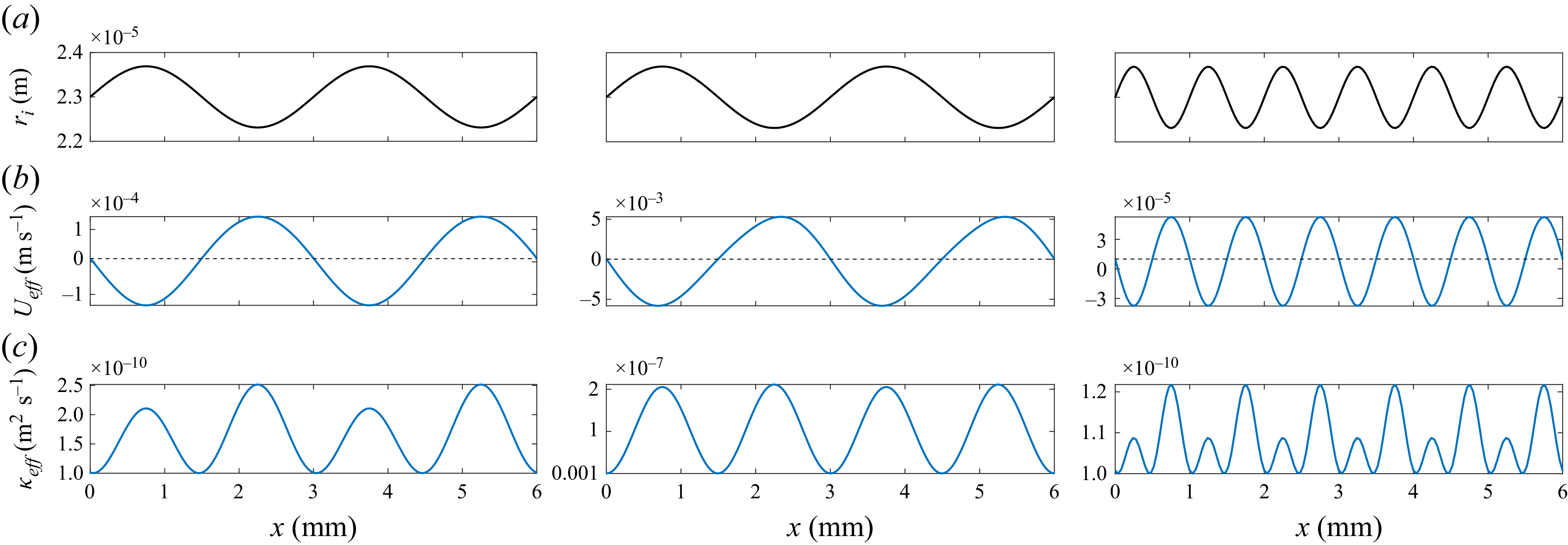


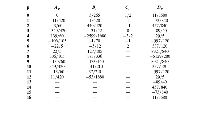

 Open access