


1. Introduction
The lowest limb of the ocean meridional overturning circulation is influenced by bottom topography and in some places channelled through narrow gaps. In some cases, ocean basins are connected by two or more deep passages. Examples include the Denmark Strait/Iceland Scotland Ridge/Faroe Bank Channel system separating the Nordic Seas from the North Atlantic Ocean, the Vema and Hunter Channels separating the Argentine and Brazil Basins and the Chain and Romanche Fracture Zones separating basins lying to the west and east of the mid-Atlantic Ridge. All of these passages contain topographic sills that the passing dense water spills over and that exert hydraulic control. The partitioning of the volume transport between the passages depends on factors such as the relative sill heights and passage widths, the broader circulation patterns that exist upstream of the sills, frictional bottom drag and possibly other factors.
A particularly representative and important example of deep flow in multiple passages occurs in the central Pacific at around 9  $^\circ$S, where the entire northward flow of Antarctic bottom water is funnelled through a set of parallel gaps, primarily the Samoan Passage but also a small gap in the Robbie Ridge to the west and a broad passage to the east of the Manihiki Plateau (figure 1b). A volume transport of 6.0 Sv (
 $1\ {\rm Sv} \equiv 10^6 {\rm m}^3\ {\rm s}^{-1}$) for the Samoan Passage was estimated from direct current meter measurements by Roemmich, Hautala & Rudnick (Reference Roemmich, Hautala and Rudnick1996) and Rudnick (Reference Rudnick1997), while a more recent field campaign resulted in an estimate of 5.4 Sv (Voet et al. Reference Voet, Alford, Girton, Carter, Mickett and Klymak2016). Roemmich et al. (Reference Roemmich, Hautala and Rudnick1996) also made hydrography-based transport estimates for the other gaps and found 1.1 Sv for Robbie Ridge and 2.8 Sv for the flow around the Manihiki Plateau. The Samoan Passage itself is complex and contains a number of branching channels with several sills. The dense flows in the various channels are observed to spill over the various sills, suggesting hydraulic control, and some of the highest levels of energy dissipation and mixing are found in the lee of the sills (Alford et al. Reference Alford, Girton, Voet, Carter, Mickett and Klymak2013; Voet et al. Reference Voet, Girton, Alford, Carter, Klymak and Mickett2015; Carter et al. Reference Carter, Voet, Alford, Girton, Mickett, Klymak, Pratt, Pearson-Potts, Cusack and Tan2019; Cusack et al. Reference Cusack, Voet, Alford, Girton, Carter, Pratt, Tan and Pearson-Potts2019). On the other hand, the 2.8 Sv of flow that passes to the east of Manihiki is observed to be concentrated in a deep western boundary current (Roemmich et al. Reference Roemmich, Hautala and Rudnick1996), one that is not constrained by a channel geometry. Although this flow encounters some deep ridges, model simulations (Pratt et al. Reference Pratt, Voet, Pacini, Tan, Alford, Carter, Girton and Menemenlis2019) suggest that it flows around, rather than over, the ridges and thus does not experience hydraulic control.
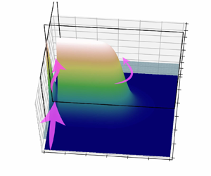
(a) Schematic picture of the circulation integral. Upstream boundary flow enters the channel and causes perturbations in terms of Kelvin waves to circle the island counter-clockwise and re-enter the channel from downstream. (b) Topography of the Samoan Passage and Manihiki Plateau region. Transports estimated from a hydrographic campaign (violet dots) across Robbie Ridge, Samoan Passage and to the east of the Manihiki Plateau by Roemmich et al. (Reference Roemmich, Hautala and Rudnick1996) are marked. The southernmost arrow shows the total transport, indicating the deep western boundary current. Panels (c) and (d) show cross-section bathymetry structures at the sill of the western and eastern paths (red sections in (b)).

These applications raise some broad questions concerning the nature of hydraulics when the incoming flow branches into multiple passages. This work mainly focuses on the hydraulics of the flow that splits around an island. In this case, a narrow channel to the west of the island and a broad passage to the east of the island form a two-passage system (figure 1a). Hydraulic control generally implies that a sill or width constriction (or both) chokes the flow and thereby exerts an influence that extends far upstream. This means that upstream conditions cannot be specified independently of the geometric conditions (sill height, channel width, etc.) at the most constricted section. Upstream influence can be demonstrated (e.g. Baines Reference Baines1995; Pratt & Chechelnitsky Reference Pratt and Chechelnitsky1997) by establishing a hydraulically controlled steady state and then raising the sill level slightly. The flow then is choked to a greater degree and a transient disturbance is produced that propagates upstream and alters the conditions there. In models of hydraulics with rotation, most notably that of Gill (Reference Gill1977), this disturbance takes the form of a Kelvin wave that is trapped to one of the sidewalls of the channel. For our Southern Hemisphere application, a Kelvin wave propagates with the wall to its left, and an upstream-propagating wave generated within the channel would therefore be trapped to the eastern wall of the channel, also the boundary of the island. The wave would travel counter-clockwise around the island and re-enter the channel from downstream, with unknown consequences. Conditions far upstream would not be influenced, and one would presumably be free to set them independently of any consideration for the geometric conditions in the channel.
A feature that makes the Samoan Passage application novel is that the main branch of the throughflow (that through the Samoan Passage) is hydraulically controlled, and subject to elevated levels of turbulence that typically occur in overflows, whereas the eastern branch is not. Is this dynamically consistent? An argument against such a scheme can be expressed using Kelvin's circulation theorem, written for a streamline that coincides with the boundary of the Manihiki Plateau ( $C_l$)
 \begin{equation} \frac{\partial}{\partial t}\oint_{C_l}\boldsymbol{u}\boldsymbol{\cdot}\boldsymbol{l}\,\mathrm{d}s +\oint_{C_l}(f+\zeta)\boldsymbol{u}\boldsymbol{\cdot}\boldsymbol{n}\,\mathrm{d}s =\delta{B}+\oint_{C_l}\boldsymbol{D}\boldsymbol{\cdot}\boldsymbol{l}\,\mathrm{d}s.\end{equation}
 The above can be obtained by integrating the tangential component of the shallow-water equations (Pratt et al. Reference Pratt, Voet, Pacini, Tan, Alford, Carter, Girton and Menemenlis2019), which assume the flow is contained in a single, homogeneous bottom layer. Here,  $\boldsymbol {u}$ is the horizontal velocity of the flow,
  $f$ is the Coriolis parameter,
  $\zeta$ is the relative vorticity of the flow. The unit vectors
  $\boldsymbol {l}$ and
  $\boldsymbol {n}$ are tangent and normal to the contour
  $C_l$ that starts and ends immediately upstream and downstream of a hypothetical hydraulic jump, and
  $s$ is the arc length measured positive in the counter-clockwise direction (figure 1a). The second term on the left-hand side of (1.1) is zero due to the no-normal-flow condition along
  $C_l$. The effect of bottom friction
  $\boldsymbol {D}$ is represented by its integral along
  $C_l$, and the effect of energy dissipation in a possible hydraulic jump is represented by the drop
  $\delta B$ in the Bernoulli function across the jump. Most rotating hydraulic theories assume that
  $\boldsymbol {D}$ is zero, but a finite value of
  $\delta {B}$ is still permitted in acknowledgement that a hydraulically controlled flow generally has supercritical flow downstream of the sill, and that this supercritical flow undergoes a transition back to subcritical via a dissipative jump. If the flow is controlled in the Samoan Passage, but not on the eastern side of the Manihiki Plateau, then a single jump will occur and
  $\delta {B}$ will be positive. In this case, a steady state cannot exist in the absence of bottom drag: indeed the flow would develop an accelerating, counter-clockwise circulation around the island. Thus, a steady-state flow that is inviscid, at least away from hydraulic jumps, can apparently not be controlled within one branch, but not the other. A steady state is possible if both branches are hydraulically controlled and both contain hydraulic jumps that produce the same
  $\delta {B}$ along the wall of the island. Alternatively, a steady state with hydraulic control in just one passage is possible if frictional drag along the alternative pathway is sufficiently large.
In order to explore these issues more deeply, we consider an idealized, shallow-water system with a single channel, bounded by a sidewall to the west and by an island or a deep-sea plateau (referred to as the ‘island’) to the east. For simplicity, the Robbie Ridge gap is disregarded and the multiple channels within the Samoan Passage are combined into a single channel. The flow is confined to a homogeneous deep layer and is fed by a northward boundary current that is trapped on the western sidewall. The channel contains a shallow sill that acts to hydraulically control the flow, whereas the abyssal plane to the east of the island has no sills or ridges. We assume that the flow has uniform potential vorticity, at least upstream of any hydraulic jumps, and our analytical model is an extension to the Gill (Reference Gill1977) hydraulic model for uniform (and non-zero) potential vorticity. The model flow contains Kelvin waves but not potential vorticity waves. Southern Hemisphere rotation is assumed, meaning that a Kelvin wave propagates with the wall to its left. In addition to the traditional, idealized topography in which sidewalls are vertical and signal transmission is due to Kelvin waves, we will consider the more realistic case in which the bottom topography varies continuously and the layer thickness goes to zero at the edges. Kelvin waves are then replaced by a frontal wave (Stern Reference Stern1980) whose properties are described in detail in Pratt & Whitehead (Reference Pratt and Whitehead2008). We will also consider numerical models for the latter type of topography.
In addition to the practical matter of predicting how the deep transport is partitioned between the channel and the eastern abyssal plain from our extended theory (§ 2), we wish to explore several conceptual issues using numerical models (§ 3). To begin with, we wish to determine whether and under what circumstances a steady-state solution is possible. We also wish to examine hydraulic transitions in the channel, including hydraulic jumps, at least to the extent possible within the confines of the model. In addition, we wish to better understand the conditions that support a steady state, and to examine how the upstream influence is altered in such a state. Finally, we wish to discuss the hydraulic control of the channel flow responding to more than one pathway (e.g. the Samoan Passage deep flow splitting between two major pathways) (Whitehead Reference Whitehead2003; Girton et al. Reference Girton2019). We will go beyond the traditional idealized topography in which sidewalls are vertical and signal transmission is due to Kelvin waves. We will do so using a more realistic topography in which the channel has a parabolic cross-section allowing the layer thickness to vanish at each edge.
2. Theory for rotating hydraulic transport
The hydraulics of a steady, single-layer flow with uniform (but non-zero) potential vorticity in a rotating channel with rectangular cross-section was described by Gill (Reference Gill1977). In his model, the flow is assumed to funnel from a wide upstream basin through a single narrow passage into the downstream basin. For flows that are hydraulically controlled, either by a topographic sill located within the narrow channel, or by the narrows itself, prediction of the volume transport is one of the fundamental goals. In particular, one would like to predict the total transport given certain key topographic information such as the height of the sill, along with other information on upstream conditions. Gill (Reference Gill1977) showed that the flow is confined to boundary currents along each wall, and that in the upstream reservoir these currents are separated by a wide, stagnant interior region. He chose to characterize the upstream state by the layer depth within the stagnant region and by the value of the transport streamfunction there. The latter specifies how the total transport is partitioned between the two boundary currents. In practice, the interior value of the transport streamfunction is not easy to observe and so alternative formulations of the upstream condition have been suggested (Whitehead & Salzig Reference Whitehead and Salzig2001; Whitehead Reference Whitehead2003). The situation depicted in figure 1 is fundamentally different because there is no upstream influence, meaning that one is free to impose an upstream condition with an arbitrary volume transport. The object is no longer to calculate the total transport but rather to predict how it is partitioned between the channel and the wide passage to the east. In the case of the Samoan Passage, the upstream flow takes the form of a broad, northward deep western boundary current which is trapped to the Tonga-Kermadec Ridge (Warren & Voorhis Reference Warren and Voorhis1970).
We next extend Gill's shallow-water model to the domain bounded to the west by a wall ( $x=0$), and containing a channel that is bounded to the west by that wall and to the east by an island (figure 2a). In view of the Samoan Passage application, we assume Southern Hemisphere rotation, so that the value of the Coriolis parameter
  $f<0$. The circulation is fed from the south by a boundary current that flows northward (positive
  $y$-direction) along the western wall. The domain can be roughly split into three parts: the upstream basin, the channel and east of the island. The bottom in the upstream basin and the region to the east of the island are assumed to be flat and bounded by vertical walls. Far to the east, the layer is assumed to be stagnant, and with constant thickness
  $D_\infty$ (figure 2b), also known as the potential depth. The most important horizontal length scale is the Rossby radius of deformation (
 $L_D=\sqrt {(g'D_\infty )}/|f|$) based on the potential depth. As Gill (Reference Gill1977) showed, all boundary currents will have this width, regardless of the local layer depth. We also employ the approximations, common in hydraulics, that the width of the channel and the bottom topography vary in the along-channel (
 $y$) direction over a scale that is long compared with
  $L_D$. The cross-channel velocity and fluid acceleration are then arguably much smaller in magnitude than the along-channel counterparts, implying that the dynamics is semi-geostrophic. The theory for a controlled flow with uniform potential vorticity is developed for both a channel with a rectangular cross-section (figure 2c), in which it is possible for the fluid depth to vanish and the flow to separate at the eastern wall, and also for a channel with parabolic cross-section (figure 2d), for which the layer thickness along each edge is always zero. We disregard friction for the time being but will introduce it in the numerical simulations. The treatment proceeds using variables that have been rendered non-dimensional using a generic depth scale
  $D$ for layer thickness
  $d$ and topographic elevation
  $h$, a corresponding Rossby radius
  $L_d=\sqrt {(g'D)}/|f|$ for the cross-channel distance
  $x$ (usually smaller than
  $L_D$ defined by the potential depth) and the long gravity wave speed
  $\sqrt {(g'D)}$ for the northward velocity
  $v$. The constant
  $g'$ represents the gravitational acceleration, reduced in proportion to the relative density difference between the lower (active) layer and overlying, less dense fluid (i.e. the so-called ‘reduced gravity’
  $g'=g({\Delta \rho }/{\rho _0})$). In this paper, star superscripts are used to denote dimensional variables (represented by
  $()^*$). Examples of dimensionless variables include
  $d=d^*/D$,
  $h=h^*/D$,
  $x=x^*/L_d$,
  $v=v^*/\sqrt {g'D}$. Although the Southern Hemisphere rotation is assumed throughout the paper, the theory is easy to be adapted to Northern Hemisphere applications. The following subsections develop predictions of the partitioning of transport between two passages, one narrow and containing a sill and the other broad and with a flat bottom. We first explore the case in which the narrow channel has a rectangular cross-section and then proceed to the case of a parabolic cross-section.
(a) An overlook sketch of a two-passage system. A narrow channel is located between the western boundary and an island, leaving a vast passage to the east of the island. (b) The cross-section of the upstream basin. The rectangular (c) and parabolic (d) cross-sections of the channel.

2.1. Rectangular channel theory
As in the Gill (Reference Gill1977) model, the potential vorticity  $q^*={(f+{\partial v^*}/{\partial x^*}-{\partial v^*}/{\partial y^*})}/{d^*}$ is assumed to be constant, eliminating Rossby waves from consideration. The value of the potential vorticity may be obtained by evaluating the expression for potential vorticity in the stagnant region far to the east of the boundaries, where the dimension depth is
  $D_\infty$, and thus
  $q^*={f}/{D_\infty }$. The scale for potential vorticity is
  ${|f|}/{D}$.
The non-dimensional expression for the semigeostrophic potential vorticity q in a Southern Hemisphere channel is then
 \begin{equation} q=\frac{-1+\dfrac{\partial v}{\partial x}}{d}={-}\frac{D}{D_\infty}. \end{equation}
The semigeostrophic approximation also requires that the northward velocity is geostrophically balanced
 \begin{equation} v={-}\frac{\partial (d+h)}{\partial x}. \end{equation}
Assuming the bottom elevation  $h(y)$ in the along-channel direction and eliminating v between these two yields a relationship for the cross-channel (x) structure of the layer thickness
  $d$
$d$
 \begin{equation} \frac{\partial^2 d}{\partial x^2} - |q|d ={-}1. \end{equation}
 Since there is no upstream influence in our multi-passage system, the western boundary current can be defined independently and can solely represent the upstream condition. Assuming that the upstream basin is infinitely wide compared with the Rossby radius of deformation in the upstream basin  $L_D$, the solution of flow along the western wall (
 $x=0$) in the upstream region may be written as
 \begin{equation} \left. \begin{array}{c@{}}
d(x)=|q|^{{-}1}+[d(x=0)-|q|^{{-}1}]\,{\rm
e}^{-|q|^{1/2}x},\\ v(x)=|q|^{1/2}[d(x=0)-|q|^{{-}1}]\,{\rm
e}^{-|q|^{1/2}x}. \end{array}\right\}
\end{equation}
\begin{equation} \left. \begin{array}{c@{}}
d(x)=|q|^{{-}1}+[d(x=0)-|q|^{{-}1}]\,{\rm
e}^{-|q|^{1/2}x},\\ v(x)=|q|^{1/2}[d(x=0)-|q|^{{-}1}]\,{\rm
e}^{-|q|^{1/2}x}. \end{array}\right\}
\end{equation}
The solutions of (2.3) in the channel are given by
 \begin{equation} \left. \begin{array}{c@{}}
d(x)=|q|^{{-}1}+\hat{d}\dfrac{\sinh[|q|^{1/2}(x-x_0)]}{\sinh(\tfrac{1}{2}|q|^{1/2}w)}
+(\bar{d}-|q|^{{-}1})\dfrac{\cosh[|q|^{1/2}(x-x_0)]}{\cosh(\tfrac{1}{2}|q|^{1/2}w)},\\
v(x)=|q|^{1/2}\left[\hat{d}\dfrac{\cosh[|q|^{1/2}(x-x_0)]}{\sinh(\tfrac{1}{2}|q|^{1/2}w)}
+(\bar{d}-|q|^{{-}1})\dfrac{\sinh[|q|^{1/2}(x-x_0)]}{\cosh(\tfrac{1}{2}|q|^{1/2}w)}\right],
\end{array}\right\} \end{equation}
\begin{equation} \left. \begin{array}{c@{}}
d(x)=|q|^{{-}1}+\hat{d}\dfrac{\sinh[|q|^{1/2}(x-x_0)]}{\sinh(\tfrac{1}{2}|q|^{1/2}w)}
+(\bar{d}-|q|^{{-}1})\dfrac{\cosh[|q|^{1/2}(x-x_0)]}{\cosh(\tfrac{1}{2}|q|^{1/2}w)},\\
v(x)=|q|^{1/2}\left[\hat{d}\dfrac{\cosh[|q|^{1/2}(x-x_0)]}{\sinh(\tfrac{1}{2}|q|^{1/2}w)}
+(\bar{d}-|q|^{{-}1})\dfrac{\sinh[|q|^{1/2}(x-x_0)]}{\cosh(\tfrac{1}{2}|q|^{1/2}w)}\right],
\end{array}\right\} \end{equation}
where  $x_0$ is at the centre of the channel,
  $w$ is the width of the channel,
 \begin{equation} \bar{d}=\frac{d\left(x_0-\dfrac{w}{2}\right)+d\left(x_0+\dfrac{w}{2}\right)}{2}\quad {\rm and}\quad \hat{d}=\frac{-d\left(x_0-\dfrac{w}{2}\right)+d\left(x_0+\dfrac{w}{2}\right)}{2}, \end{equation}
represent the average and difference of the flow thickness at walls. The corresponding average and difference of  $v$ at the walls are given by
 \begin{equation} \left. \begin{array}{c@{}}
\bar{v}=\dfrac{v\left(x_0-\dfrac{w}{2}\right)+v\left(x_0+\dfrac{w}{2}\right)}{2}={-}|q|^{1/2}T^{{-}1}\hat{d},\\
\hat{v}=\dfrac{-v\left(x_0-\dfrac{w}{2}\right)+v\left(x_0+\dfrac{w}{2}\right)}{2}={-}|q|^{1/2}T(\bar{d}-|q|^{{-}1}),
\end{array}\right\},
\end{equation}
\begin{equation} \left. \begin{array}{c@{}}
\bar{v}=\dfrac{v\left(x_0-\dfrac{w}{2}\right)+v\left(x_0+\dfrac{w}{2}\right)}{2}={-}|q|^{1/2}T^{{-}1}\hat{d},\\
\hat{v}=\dfrac{-v\left(x_0-\dfrac{w}{2}\right)+v\left(x_0+\dfrac{w}{2}\right)}{2}={-}|q|^{1/2}T(\bar{d}-|q|^{{-}1}),
\end{array}\right\},
\end{equation}
where  $T=\tanh (\frac {1}{2}|q|^{1/2}w)$.
We then define a transport streamfunction  $\varPsi$ from the along-channel velocity
  $vd={\partial \varPsi }/{\partial x}$. Since the interior of the upstream basin is stagnant, the streamfunction there is constant. For convenience, we take
  $\varPsi =0$ in the interior basin (
 $x\gg 0$), which allows
  $\varPsi$ at any streamline to be given by the flow flux between that streamline and the stagnant basin interior. For example, the western wall can be treated as a single streamline extending from the upstream basin toward the channel because of the condition of no normal flux. Given the transport
  $Q$ of the western boundary current in the upstream basin, we find
  $\varPsi =-Q$ along the western wall. Here,
  $Q$ can be approximated by integrating
  $vd\equiv -d({\partial d}/{\partial x})$ from
  $x=0$ to a point in the basin interior where
  $d(x\gg 0)\approx |q|^{-1}$ and
  $v(x\gg 0)\approx 0$
 \begin{equation} Q\simeq{-}\frac{|q|^{{-}2}-d^2(x=0)}{2}.\end{equation}
From (2.4) and (2.8), we get  $d(x=0)\simeq \sqrt {2Q+\!|q|^{-2}}$ and
  $v(x=0)\simeq |q|^{1/2}(\sqrt {2Q+\!|q|^{-2}} -\!|q|^{-1})$. For an inviscid flow that has a constant
  $q$, the Bernoulli function
  $B\!=\!{v^2}/{2}\!+d\!+h$ is conserved along streamlines (Crocco Reference Crocco1937)
 \begin{equation} q=\frac{\mathrm{d}B}{\mathrm{d}\varPsi}.\end{equation}
Integrating (2.9) from the basin interior where  $B(x\gg 0)\approx |q|^{-1}$ and utilizing
  $\varPsi (x=0)=-Q$, the Bernoulli function at the western wall is determined by
  $Q$ and
  $q$
$q$
 \begin{equation} B(x=0)\simeq|q|Q+|q|^{{-}1}. \end{equation}
 The no-normal-flux boundary condition also ensures that the island boundary is a streamline ( $\varPsi =-\varPsi _0$). If the upstream inflow splits as it approaches the entrance of the channel, a streamline originating from the upstream western boundary current area would meet the island boundary at a stagnation point upstream of the sill (
 $P$ in figure 2a). The streamfunctions at that streamline and at the island boundary share the same value. It is worth noting that a stagnation point located downstream of the sill on the island boundary is also possible, in which case the flow immediately to the east of the splitting streamline has to turn around as it approaches the stagnation point. An upstream/downstream stagnation point corresponds to a uniformly northward flow/reversal flow in the eastern part of the channel. In regions upstream of and at the sill, where the flow cannot undergo a hydraulic jump, we may assume that
  $v$ and
  $d$ are continuous and compute the transport through the channel
  $Q_1$ by integrating
  $-d({\partial d}/{\partial x})$ between the two sidewalls of the channel
 \begin{equation} Q_1={-}2\hat{d}\bar{d}. \end{equation}
From definition,  $\varPsi _0=Q-Q_1=Q+2\hat {d}\bar {d}$.
The average Bernoulli function in the channel
 \begin{align} \bar{B}&=\frac{B\left(x_0-\dfrac{w}{2}\right)+B\left(x_0+\dfrac{w}{2}\right)}{2}\nonumber\\ &=\frac{v^2\left(x_0-\dfrac{w}{2}\right)+v^2\left(x_0+\dfrac{w}{2}\right)}{4} +\frac{d\left(x_0-\dfrac{w}{2}\right)+d\left(x_0+\dfrac{w}{2}\right)}{2}+h, \end{align}
can be simplified by substituting  ${(v^2(x_0-{w}/{2})+v^2(x_0+{w}/{2}))}/{2}$ with
  $\bar {v}^2+\hat {v}^2$ and employing (2.7)
 \begin{equation} \bar{B}=\tfrac{1}{2}|q|[T^{{-}2}\hat{d}^2+T^2(\bar{d}-|q|^{{-}1})^2]+\bar{d}+h. \end{equation}
Also,  $\bar {B}$ can be rearranged as
  ${(B(x_0+{w}/{2})-B(x_0-{w}/{2}))}/{2}+B(x_0-{w}/{2})$. Since
  $q$ is constant, the first term can be written in terms of
  $Q_1$ and
  $q$ following (2.9)
 \begin{equation} \bar{B}={-}\frac{|q|Q_1}{2}+B\left(x_0-\frac{w}{2}\right),\end{equation}
where  $B(x_0-{w}/{2})$ is conserved along the streamline at the western wall, and thus can be expressed by
  $Q$ and
  $q$ from (2.10).
Combining (2.13) and (2.14) by substituting (2.10) and (2.11) relates a single unknown flow property in the channel  $\bar {d}$ to the local geometric parameters
  $h, w$ by the equation
 \begin{align} \mathcal{G}(\bar{d}\,|\,h;w;q;Q;Q_1) & = \frac{Q^2_1}{4T^2\bar{d}^2}+T^2(\bar{d}-|q|^{{-}1})^2+2|q|^{{-}1}\bar{d}\nonumber\\ &\quad -2|q|^{{-}1}(|q|Q+|q|^{{-}1}-h)+Q_1=0. \end{align}
We are primarily interested in flows that are hydraulically controlled by a sill (maximum bottom elevation) that lies within the channel. Such flows approach the sill in a subcritical state that allows upstream propagation by at least one of the waves permitted under the semigeostrophic approximation. Upon reaching the sill, the flow undergoes a transition to a supercritical state in which the same wave propagates downstream. At the transition the wave is stationary, meaning that it is technically possible to locally alter the steady flow without changing the upstream conditions. As shown by Gill (Reference Gill1977), this critical condition is given by  ${\partial \mathcal {G}}/{\partial \bar {d}}|_c=0$ and leads here to
 \begin{equation} (1-T^2_c)|q|^{{-}1}+T^2_c\bar{d}_c=\frac{Q^2_{1_c}}{4T_c^2\bar{d}_c^3},\end{equation}
where the subscript  $()_c$ denotes quantities evaluated at the critical section. Elimination of
  $\bar {d}_c$ between (2.15), evaluated at the critical section, and (2.16) determines the critical transport in the channel
  $Q_{1_c}$ in terms of the topography of the critical section
  $w_c$,
  $h_c$, and the upstream conditions
  $q$ and
  $Q$. In the dimensionalized form, the determination of
  $Q^*_{1_c}$ depends on
  $w^*_c$,
  $h^*_c$,
  $D_\infty$ and
  $Q^*$.
It is possible that the flow in the channel may become separated from the eastern wall and thereby take on a width  $w_e$ that is less than the local channel width. In this case, it is easy to show that
  $Q_1=2\bar {d}^2$, so that
  $\bar {d}$ becomes fixed, and it is better to use
  $w_e$ as the primary variable characterizing the flow. Equation (2.15) is now replaced by
 \begin{align} \mathcal{G}(T_e\,|\,\bar{d};h;q;Q) & = T_e^2(\bar{d}-|q|^{{-}1})^2+T_e^{{-}2}\bar{d}^2+2\bar{d}^2+2|q|^{{-}1}\bar{d}\nonumber\\ &\quad -2|q|^{{-}1}(|q|Q+|q|^{{-}1}-h)=0, \end{align}
where  $T_e=\tanh (|q|^{1/2}w_e/2)$. The width and the transport of a separated flow under hydraulic control can be solved by substituting the critical condition
  ${\partial \mathcal {G}}/{\partial T_e}|_c=0$ into (2.17).
2.2. Parabolic channel theory
The need to distinguish between separated and non-separated states is a consequence of the unrealistic assumption of vertical sidewalls and is eliminated by the use of a channel cross-section with continuously varying bottom elevation. A parabolic cross-section is almost invariably a better approximation to conditions in nature and has been considered by Borenäs & Lundberg (Reference Borenäs and Lundberg1986) within the context of uniform potential vorticity. We do, however, continue to assume that the upstream basin is bounded by vertical walls, and we employ the same streamline configuration as in the rectangular channel case. Therefore, the upstream condition is specified by the value of the potential vorticity and by the transport of the upstream western boundary current. Now we give the derivation of the analogue of (2.15) and (2.16) for a parabolic channel and the procedure for estimating the partitioning of inflow transport.
Consider a channel with parabolic cross-sectional bottom elevation, in dimensional variables
 \begin{equation} h^*=h^*_0+{\alpha}(x^*-x_0^*)^2,\end{equation}
where  $h^*_0$ is the height of the channel bottom at its deepest point, and has value zero in the upstream bottom. Equation (2.18) is non-dimensionalized using
  $L_d=\sqrt {g'D}/|f|$ for the cross-sectional dimension
  $x$ and
  $D$ for the bottom topography
  $h$ to yield
 \begin{equation} h=h_0+\frac{(x-x_0)^2}{r}, \end{equation}
where  $r={|f|^2}/{g'\alpha }$ is the non-dimensional shape parameter, large for a ‘wide’ channel (one for which the radius of curvature
  ${\gg }L_d$).
The non-dimensional governing equations for the flow in a parabolic channel are given by
 \begin{equation} \left. \begin{array}{c@{}}
\displaystyle\dfrac{\partial^2 d}{\partial x^2} - |q|d
={-}1-2r^{{-}1},\\ \displaystyle v={-}\dfrac{\partial
(d+h)}{\partial x}, \end{array}\right\}
\end{equation}
\begin{equation} \left. \begin{array}{c@{}}
\displaystyle\dfrac{\partial^2 d}{\partial x^2} - |q|d
={-}1-2r^{{-}1},\\ \displaystyle v={-}\dfrac{\partial
(d+h)}{\partial x}, \end{array}\right\}
\end{equation}
which can be solved analytically given the boundary conditions  $d(x_0-a)=d(x_0+b)=0$, where
  $x=x_0-a$ and
  $x=x_0+b$ are the locations where the interface intersects the bottom (figure 2d)
 \begin{equation} \left. \begin{array}{c@{}}
d(x)=\dfrac{1+2r^{{-}1}}{|q|\sinh(|q|^{1/2}(a+b))}[\sinh(|q|^{1/2}(x-x_0-b))\\
\hspace{8pt}-\sinh(|q|^{1/2}(x-x_0+a))]+\dfrac{1+2r^{{-}1}}{|q|},\\
v(x)={-}\dfrac{1+2r^{{-}1}}{|q|^{1/2}\sinh(|q|^{1/2}(a+b))}[\cosh(|q|^{1/2}(x-x_0-b))\\
-\cosh(|q|^{1/2}(x-x_0+a))]-2r^{{-}1}(x-x_0).
\end{array}\right\} \end{equation}
\begin{equation} \left. \begin{array}{c@{}}
d(x)=\dfrac{1+2r^{{-}1}}{|q|\sinh(|q|^{1/2}(a+b))}[\sinh(|q|^{1/2}(x-x_0-b))\\
\hspace{8pt}-\sinh(|q|^{1/2}(x-x_0+a))]+\dfrac{1+2r^{{-}1}}{|q|},\\
v(x)={-}\dfrac{1+2r^{{-}1}}{|q|^{1/2}\sinh(|q|^{1/2}(a+b))}[\cosh(|q|^{1/2}(x-x_0-b))\\
-\cosh(|q|^{1/2}(x-x_0+a))]-2r^{{-}1}(x-x_0).
\end{array}\right\} \end{equation}
The volume flux  $Q_1$ can be obtained by integrating
  $-d({\partial (d+h)}/{\partial x})$ across the channel
 \begin{align} Q_1&=(a-b)\frac{1+2r^{{-}1}}{|q|r}\{2|q|^{{-}1/2}[\sinh^{{-}1}(|q|^{1/2}(a+b))\nonumber\\ &\quad -\coth(|q|^{1/2}(a+b))]+(a+b)\}, \end{align}
and the wall-average Bernoulli function in the channel is again defined by
 \begin{equation} \bar{B}=\frac{B(x_0-a)+B(x_0+b)}{2}, \end{equation}
where  $B(x_0-a)$ and
  $B(x_0+b)$ are Bernoulli functions at the western and eastern edges of the flow, respectively,
 \begin{align} \left. \begin{aligned}
B(x_0-a)&=\dfrac{1}{2}\left\{-\dfrac{1+2r^{{-}1}}{|q|^{1/2}\sinh(|q|^{1/2}(a+b))}[\cosh(|q|^{1/2}(a+b))-1]+2r^{{-}1}a
\right\}^2\\ &\quad +h_0+\dfrac{a^2}{r},\\
B(x_0+b)&=\dfrac{1}{2}\left\{-\dfrac{1+2r^{{-}1}}{|q|^{1/2}\sinh(|q|^{1/2}(a+b))}[1-\cosh(|q|^{1/2}(a+b))]-2r^{{-}1}b
\right\}^2\\ &\quad +h_0+\dfrac{b^2}{r}. \end{aligned}\right\}
\end{align}
\begin{align} \left. \begin{aligned}
B(x_0-a)&=\dfrac{1}{2}\left\{-\dfrac{1+2r^{{-}1}}{|q|^{1/2}\sinh(|q|^{1/2}(a+b))}[\cosh(|q|^{1/2}(a+b))-1]+2r^{{-}1}a
\right\}^2\\ &\quad +h_0+\dfrac{a^2}{r},\\
B(x_0+b)&=\dfrac{1}{2}\left\{-\dfrac{1+2r^{{-}1}}{|q|^{1/2}\sinh(|q|^{1/2}(a+b))}[1-\cosh(|q|^{1/2}(a+b))]-2r^{{-}1}b
\right\}^2\\ &\quad +h_0+\dfrac{b^2}{r}. \end{aligned}\right\}
\end{align}
As before, we invoke conservation of the Bernoulli function and volume flux between the upstream region, where ((2.10), (2.14)) are still valid, and the sill section of the parabolic channel. This connection is made for streamlines that originate upstream and that pass through the channel. Use of (2.22)–(2.24) leads to an equation for the width ( $a+b$) of the current
 \begin{align}
&\mathcal{G}((a+b)\,|\,h_0;r;q;Q;Q_1)\nonumber\\ &\quad =
\frac{1}{2}\left\{\frac{(1+2r^{{-}1})[\cosh(|q|^{1/2}(a+b))-1]}{|q|^{1/2}\sinh(|q|^{1/2}(a+b))}\right\}^2\nonumber\\
&\qquad
-\frac{(1+2r^{{-}1})[\cosh(|q|^{1/2}(a+b))-1]}{r|q|^{1/2}\sinh(|q|^{1/2}(a+b))}(a+b)\nonumber\\
&\qquad
+\frac{r+2}{4r^2}[(a+b)^2+(a-b)^2]+\frac{|q|Q_1}{2}-|q|Q-|q|^{{-}1}+h_0=0,
\end{align}
\begin{align}
&\mathcal{G}((a+b)\,|\,h_0;r;q;Q;Q_1)\nonumber\\ &\quad =
\frac{1}{2}\left\{\frac{(1+2r^{{-}1})[\cosh(|q|^{1/2}(a+b))-1]}{|q|^{1/2}\sinh(|q|^{1/2}(a+b))}\right\}^2\nonumber\\
&\qquad
-\frac{(1+2r^{{-}1})[\cosh(|q|^{1/2}(a+b))-1]}{r|q|^{1/2}\sinh(|q|^{1/2}(a+b))}(a+b)\nonumber\\
&\qquad
+\frac{r+2}{4r^2}[(a+b)^2+(a-b)^2]+\frac{|q|Q_1}{2}-|q|Q-|q|^{{-}1}+h_0=0,
\end{align}
where  $(a-b)$ is connected with
  $(a+b)$ via (2.22)
 \begin{align} (a-b)&=\frac{|q|rQ_1}{1+2r^{{-}1}}\{2|q|^{{-}1/2}[\sinh^{{-}1}(|q|^{1/2}(a+b))\nonumber\\ &\quad -\coth(|q|^{1/2}(a+b))]+(a+b)\}^{{-}1}. \end{align}
The dimensionalized form of (2.25) is  $\mathcal {G^*}((a^*+b^*)\,|\,h^*_0;\alpha ;D_\infty ;Q^*;Q^*_1)=0$. The critical condition can be achieved by taking
  ${\partial \mathcal {G}}/{\partial (a+b)}|_c=0$
 \begin{align} &\frac{2(1+2r_c^{{-}1})^2}{|q|^2r_c^2}[{\rm csch}(|q|^{1/2}(a+b)_c)- \coth(|q|^{1/2}(a+b)_c)]\nonumber\\ &\qquad \times \{|q|^{{-}1/2}(r_c+2)\,{\rm csch}(|q|^{1/2}(a+b)_c)[{\rm csch}(|q|^{1/2}(a+b)_c)-\coth(|q|^{1/2}(a+b)_c)]\nonumber\\ &\qquad +|q|^{{-}1/2}+(a+b)_c\,{\rm csch}(|q|^{1/2}(a+b)_c)\}+\frac{(1+2r_c^{{-}1})^2}{|q|^2r_c^2}(a+b)_c\nonumber\\ &\quad =\frac{2{\rm csch}(|q|^{1/2}(a+b)_c)[{\rm csch}(|q|^{1/2}(a+b)_c)-\coth(|q|^{1/2}(a+b)_c)]+1}{\{2q^{{-}1/2}[{\rm csch}(|q|^{1/2}(a+b)_c)-\coth(|q|^{1/2}(a+b)_c)]+(a+b)_c\}^3}Q^2_{1_c}, \end{align}
where all variables with subscript  $c$ denote quantities evaluated at the critical section. Solving the controlled volume flux
  $Q_{1_c}$ by eliminating
  $(a+b)_c$ between
  $\mathcal {G}((a+b)_c\,|\,h_{0_c};r_c;q;Q;Q_{1_c})$ and (2.27) is not easy. Instead, we solve the critical level of
  $(a+b)_c$ numerically by optimizing
  $Q_{1_c}$ while satisfying the constraints (2.25)–(2.27) using the interior-point algorithm (Byrd, Gilbert & Nocedal Reference Byrd, Gilbert and Nocedal2000).
2.3. Dependence of the flow variable on geometry
The theory described in §§ 2.1 and in 2.2 can be employed to predict the partitioning of the inflow transport  $Q$ given the upstream conditions (
 $q$ and
  $Q$) for different sill topographic parameters (
 $w_c$ and
  $h_c$ for a rectangular cross-section or
  $r_c$ and
  ${h_0}_c$ for a parabolic cross-section). Furthermore, various topographic regimes can be characterized by the different features of the flow as shown in figures 3 and 4(a). Only results for the upstream conditions
  $q=-1$ and
  $Q=0.5$ are shown, which are selected to represent the inflow upstream of the Samoan Passage (see the Samoan Passage application in more detail in § 4.1). Different
  $q$ and
  $Q$ yield qualitatively similar regime boundaries.
The theoretical critical transport  $Q_{1_c}$ in the rectangular channel is contoured as a function of the channel width
  $w_c$ and bottom height
  $h_c$ at the critical section (sill). The upstream condition is set by the potential vorticity (
 $q=-1$) and volume transport (
 $Q=0.5$) of the upstream inflow. The transport to the east of the island is
  $Q-Q_{1_c}$. Above the curve
  $Q_{1_c}=0$ the channel flow is topographically blocked; below the curve
  $Q_{1_c}=0.5$ the volume transport in the channel exceeds that of the upstream flow and the theory is considered invalid (dark shades). The flow is separated from the eastern wall to the right of the dashed curve (light shades). The triangles show the predicted
  $Q_{1_c}$ for the Samoan Passage topography.

(a) Value of  $Q_{1_c}$ as a function of
  $r_c$ and
  ${h_0}_c$ for a hydraulically controlled flow in a parabolic channel from theory (contours). The inflow has a potential vorticity of
  $q=-1$, and a transport of
  $Q=0.5$. The flow tends to be blocked by the sill in the regime of large
  ${h_0}_c$. Below the
  $Q_{1_c}=0.5$ contour is the regime where the theory becomes no longer valid (dark shades). On the right of the dashed grey curve, the predicted channel flow at the western boundary is southward, suggesting a reversal circulation (light shades). Numbers in black and red are results from the theory and numerical model, respectively; ‘nan’ (dark shades) represents null values. Insets (b–i) show the time-mean (
 $100\leq t\leq 400$) northward velocity
  $v$ (red suggesting positive) and interface height
  $d+h$ (black contours) in the channel of selected topographic parameters from the numerical simulation.

Figure 3 suggests four separate regimes. Above the  $Q_{1_c}=0$ contour, the flow is topographically blocked by the sill. In the regime below the
  $Q_{1_c}=0.5$ contour, the predicted critical transport
  $Q_{1_c}$ is larger than the inflow transport
  $Q$, meaning that part of the transport must be sourced from regions to the east or north of the island. If this is the case, the potential vorticity of the channel flow is partially set by downstream conditions, and the stagnation point (P in figure 2a) would no longer exist. We have elected not to venture into this regime since the conditions do not seem realistic. In the regime lying to the right of the dashed curve, the flow is separated from the eastern wall at the sill section. Therefore the flow is controlled only by the bottom elevation
  $h_c$ while
  $Q_{1_c}$ remains constant for an increasing
  $w_c$. However, historical laboratory experiments (Shen Reference Shen1981; Pratt Reference Pratt1987) and numerical simulations (Pratt, Helfrich & Chassignet Reference Pratt, Helfrich and Chassignet2000) have both suggested that hydraulic control of separated sill flows is very difficult to establish, so this regime may only exist in theory. In the regime lying between the
  $Q_{1_c}=0$ and
  $Q_{1_c}=0.5$ contours, and on the left of the separation curve, the flow in the channel is hydraulically controlled and
  $Q_{1_c}$ decreases with increasing
  $h_c$ and decreasing
  $w_c$.
As shown in figure 4(a), there are four topographic regimes for flow in the channel with a parabolic cross-section. Similar to the rectangular cross-section case, the flow is likely to be blocked by the sill in the regime of large  ${h_0}_c$ (especially when
  ${h_0}_c\geq 1.4$), where the theory predicted
  $Q_{1_c}$ is very close to zero. In the topographic regime below the
  $Q_{1_c}=0.5$ contour, the predicted
  $Q_{1_c}$ is larger than
  $Q$, and the theory is again considered invalid. Different from the rectangular cross-section case, there is no boundary separation for a flow in a channel with varying topography. However, for a wide channel with
  $r_c$ lying on the right of the dashed curve, the theory produces a southward flow at the western boundary of the channel, suggesting a reversal circulation. One may imagine that a stagnation point must be located upstream of the sill at the western boundary, which connects the streamline following the western boundary and the streamline that constitutes the other boundary of the reversal circulation. In the final regime (left of the dashed curve, above
  $Q_{1_c}=0.5$ and moderate
  ${h_0}_c$), the predicted channel flow is hydraulically controlled.
3. Numerical exploration of time-dependent hydraulic adjustment
The theoretical model described in § 2 is limited to a steady, semigeostrophically balanced, inviscid channel flow. Most importantly, it assumes that the flow in the channel is hydraulically controlled under certain given upstream conditions despite the possible influence from the flow to the east of the island. As sketched in figure 1(a), a Kelvin wave or a frontal wave may propagate into the channel from downstream and, if it is large enough, alter the flow at the sill. In this section, we turn to a numerical model and show that persistent hydraulic control in the channel requires a certain amount of frictional drag acting on the flow to the east of the island. This result is anticipated by the circulation integral described in the introduction. Since a varying bottom topography is more realistic than vertical walls in the ocean, numerical experiments in this section are designed only to study flow passing a parabolic channel.
3.1. Numerical method
The numerical model used for this study was first described in Helfrich, Kuo & Pratt (Reference Helfrich, Kuo and Pratt1999) in a study of the nonlinear Rossby adjustment problem in a rotating channel. The model solves the non-dimensional shallow-water equations in flux form
 $$\begin{gather} \frac{\partial}{\partial t}(ud)+\frac{\partial}{\partial x}\left(u^2d+\frac{1}{2}d^2\right)+\frac{\partial}{\partial y}(uvd)-{\rm sign}(f)vd+d\frac{\partial h}{\partial x}={-}\lambda{ud}, \end{gather}$$
 $$\begin{gather}\frac{\partial}{\partial t}(vd)+\frac{\partial}{\partial y}\left(v^2d+\frac{1}{2}d^2\right)+\frac{\partial}{\partial x}(uvd)+{\rm sign}(f)ud+d\frac{\partial h}{\partial y}={-}\lambda{vd}, \end{gather}$$
 $$\begin{gather}\frac{\partial d}{\partial t}+\frac{\partial }{\partial x}(ud)+\frac{\partial }{\partial y}(vd)=0, \end{gather}$$
where  $\lambda$ is the Rayleigh friction coefficient. Here, we choose to work with a linear parameterization of the bottom friction (or the ‘Rayleigh friction’ representing the momentum loss in a bottom Ekman layer) because it is more numerically stable than the more commonly used quadratic bottom drag. The model allows for ‘dry regions’ (defined by layer thickness
  $d<10^{-4}$) and permits the formation of sharp hydraulic jumps and bores, at the same time ensuring that the proper shock-joining conditions on mass and momentum flux are satisfied. The model assumes constant background rotation (
 $f$-plane physics) and the
  $x$-direction (cross-channel) and
  $y$-direction (along-channel) continue to act as eastward and northward coordinates. The non-dimensional variables in the model have been formed using slightly different scaling than that given in the theory. In particular (i) lengths in the
  $x$-direction and the
  $y$-direction are both scaled by the Rossby radius of deformation
  $L_d$ and therefore
  $u$ and
  $v$ are both scaled by the free long gravity wave speed
  $\sqrt {g'D}$ (i.e. non-semigeostrophic;
  $|v/u|\sim O(1)$); (ii) the time is scaled by
  $1/|f|$ (i.e. time dependent); (iii)
  $\lambda$ is scaled by
  $|f|$.
As shown in figure 5(a), a channel with a parabolic cross-section is introduced between the island and the western boundary of the model domain (figure 5b). The channel contains an obstacle having a Gaussian shape in the along-channel direction (figure 5c)
 \begin{equation} h(x,y)=\left[h_s+\frac{(x-x_s)^2}{r_s}\right]{\rm e}^{-{(y-y_s)^2}/{2\sigma^2_s}},\quad 0\leq x\leq 2x_s, \end{equation}
where  $(x_s,y_s)$ and
  $(r_s,h_s)$ denote the location and the topographic parameters of the topographic saddle point (sill), respectively, and
  $\sigma _s$ indicates the channel length. The sloping western sidewall in the channel joins continuously to the vertical sidewalls of the western boundary north and south of the channel. A logistic function (figure 5b) makes up the sloping eastern boundary of the island, which gradually joins the sea bottom
 \begin{equation} h(x,y)=\frac{1}{1+{\rm e}^{{(x-x_i)}/{\sigma_i}}}h(0,y),\quad x>2x_s, \end{equation}
where  $x_i$ and
  $\sigma _i$ indicate the starting point of the island's eastern slope and the span of the slope, respectively.
(a) Model domain and topography. The initial layer surface ( $d+h=1$) is represented by a light blue sheet. (b) The cross-channel topography at
  $y_s=35$, looking towards downstream. The channel is parabolic. (c) The side view of a section across the deepest point in the channel, showing the along-channel Gaussian topography. The topographic parameters
  $\sigma _s$,
  $\sigma _i$ and
  $x_i$ are set to 5, 5 and 30, respectively.

We consider a set of simulations in which the flow in the interior of the domain is initially at rest, and the interface height  $d+h$ is set to unity. At
  $t=0$, a steady, northward, geostrophically balanced flow with total volume flux
  $Q=0.5$ and with potential vorticity
  $q=-1$ is introduced across the southern boundary of the model domain. The profiles of northward velocity and layer thickness take the form of the boundary current described by (2.4). The boundary conditions at the western and eastern walls of the domain are free slip and no normal flux, and radiation conditions (Orlanski Reference Orlanski1976) are used at the northern boundary of the domain. The numerical domain is 60 units in both the
  $x$-direction and the
  $y$-direction, with spacing in the
  $y$-direction of
  $\Delta y=0.1$. The cross-channel grid spacing and time steps range from (
 $\Delta x=0.1$ and
  $\Delta t=0.01$) for wide channels with
  $r_s>1$ to (
 $\Delta x=0.05$ and
  $\Delta t=0.002$) for narrow channels with
  $r_s<1$. The validity of the numerical results was tested by reducing
  $\Delta x$,
  $\Delta y$ and
  $\Delta t$ by one half and by doubling the range of
  $x$ and
  $y$ while maintaining the same channel and island geometry. The former set of experiments can better resolve features in regions of hydraulic transients (see § 3.3) but also show more oscillations near discontinuities. Besides these small oscillations, all test runs show essentially the same overall flow patterns as models used for the analysis.
3.2. Friction and no-friction experiments
Several friction and no-friction numerical runs were made for comparison with results from the theory and to explore phenomena such as hydraulic transitions and signal transmissions from downstream that are not addressed by the theory. In a no-friction experiment, the Rayleigh friction coefficient  $\lambda$ is zero everywhere in the model domain. In a friction experiment,
  $\lambda$ is set to zero between the western wall (
 $x=0$) and
  $x=15$, which includes the channel and much of the western boundary layer to keep the calculations close to the inviscid theories, whereas
  $\lambda =0.2$ is added to
  $x>15$, which includes the boundary layer on the east coast of the island.
Numerical results from two sets of topographic parameters ( $r_s=1.3$,
  $h_s=0.6$) and (
 $r_s=0.2$,
  $h_s=0.6$), which represent the Samoan Passage (see details in § 4.1) and a nominal narrow channel, respectively, are examined closely. Time series of the volume transport in the channel (
 $Q_1$) and east of the island (
 $Q_2$) were calculated at
  $y_s$=35, the latitude of both the sill and the minimum width in the channel. From inviscid theories, this topographic saddle point coincides with the critical section (i.e.
  $r_c=r_s$,
  ${h_0}_c=h_s$) had the flow becomes hydraulically controlled in the channel (Pratt & Whitehead Reference Pratt and Whitehead2008, § 1.4).
3.2.1. Persistent hydraulic control in the friction experiments
As shown in figure 6(c,d,g,h), beginning at  $t\approx 50$,
  $Q_1$ from the simulation becomes quite close to the critical value
  ${Q_1}_c$ predicted by the theory for (
 $r_c=r_s$,
  ${h_0}_c=h_s$), suggesting that the hydraulic control is established after the adjustment of Kelvin waves and frontal waves to the topography of the channel (Pratt et al. Reference Pratt, Helfrich and Chassignet2000). The constant
  $Q_1$ after
  $t\approx 50$ persists until
  $t\approx 250$, then
  $Q_1$ from the no-friction experiments starts to drop, while
  $Q_1$ from the friction experiments remains relatively unchanged. After
  $t\approx 400$, the transport calculated at the southern boundary of the model domain
  $Q$ starts to show irregular variations, which may be due to the contamination with Kelvin waves that are initialized by the errors of the radiation boundary condition at the northern boundary of the domain and propagate along the domain's eastern boundary into the upstream section. The small decrease in
  $Q_1$ after
  $t\approx 400$ in figure 6(c) is likely due to the same process. Aside from these numerical artifacts, only the friction experiments yield persistent hydraulic control, while the no-friction experiments show a continuous transport adjustment. In fact,
  $Q_1$ in figure 6(g,h) continues to decrease towards zero as we run the simulation until
  $t=2000$ (not shown). We have run experiments with
  $\lambda =0.2$ everywhere of the model domain and also found a persistent hydraulic control in the channel, except for the magnitude difference in
  $Q_1$ due to the friction-induced flow spindown (not shown).
Numerical results from the (a–d) friction experiments (Rayleigh friction added to  $x>15$) and the (e–h) no-friction experiments. (a,e) Flow speed
  $\sqrt {u^2+v^2}$ at
  $t=800$, with colour bar shown at the upper right corner of (a). The interface heights
  $d+h$ of 1.2 and 1.4 are marked with thick black contours. The bathymetry contours
  $h=0.6$ along the western boundary of the channel and around the island are shown by the cyan and green dashed curves respectively in (a) and partly in (b). (b, f) A magnified view of the modelled flow in the channel (
 $x\in [0, 6]$). Meridional velocity
  $v$ is shown in colours (red for northward flow and blue for southward flow, with colour bar shown at the lower left corner of (b)). The
  $d+h$ contours are shown at 0.1 intervals. The grey lines indicate the location of the sill. Panels (a,b,e, f) are all for topographic parameters (
 $r_s=1.3$,
  $h_s=0.6$). Volume transport time series for parameters (
 $r_s=1.3$,
  $h_s=0.6$) (c,g) and (
 $r_s=0.2$,
  $h_s=0.6$) (d,h). Here,
  $Q$,
$Q$,  $Q_1$ and
  $Q_2$ represent the transport of the flow in the upstream basin, in the channel and along the eastern flank of the island, respectively. Theory predictions
  ${Q_1}_c$ for a hydraulically controlled channel flow at (
 $r_c=r_s$,
  ${h_0}_c=h_s$) are indicated by the dashed lines.

3.2.2. Transport adjustment by frontal waves in the no-friction experiments
In order to examine the role that transients may play in the transport adjustment, we show Hovmöller diagrams of the interface height  $d+h$ along two circuits: one following the western boundary of the channel (the cyan dashed curve in figure 6a,b) and the other circling the island (the green dashed curve in figure 6a,b). Both of the circuits are isobaths with
  $h=0.6$. The coastal trapped waves that propagate along these circuits see zero layer thickness along the respective in-shore edges and are similar to the frontal waves described by Stern (Reference Stern1980). Like southern hemisphere Kelvin waves, they tend to propagate with the boundary to their left, at least in the absence of a mean flow. The Hovmöller diagrams for the west circuit figure 7(a,c), show that a set of these waves arrives in the channel prior to
  $t\approx 50$, carrying with them the initial surge in transport and establishing hydraulic control at the sill. In the friction experiments, after the hydraulic control is established,
  $d+h$ in regions upstream of and at the sill remains relatively constant with time. The closed contours downstream of the sill denote eddies (also seen in figure 6b). However, in the no-friction experiments,
  $d+h$ changes significantly in regions upstream of and at the sill after
  $t\approx 250$ and eddy formation ceases downstream of the sill.
Time evolution of the interface height ( $d+h$) at the bathymetry contour
  $h=0.6$ (a,c) along the western boundary of the channel (west circuit: cyan dashed curve in figure 6a) and (b,d) around the island (east circuit: green dashed curve in figure 6a). Panels (a,b), (c,d) show results from the friction and no-friction experiments, respectively. Both experiments use topographic parameters (
 $r_s=1.3$,
  $h_s=0.6$). The
  $y$ coordinate in (a,c) is the distance from the most upstream point of the west circuit, in (b, d) is the distance from P1 around the island in a counter-clockwise direction. The contour interval is 0.05. The frontal waves that propagate counter-clockwise along the island and penetrate the channel from downstream are highlighted in a grey arrow in (d) with the phase speed marked (
 $c=0.3$).

The evolving interface elevation  $d+h$ along the east circuit is shown in figures 7(b) and 7(d). For the case without friction, figure 7(d), the leading edge of frontal waves circles the island (counter-clockwise along segment P1–P2) with a speed of
  $c\approx 0.3$ and penetrates back up into the channel at
  $t\approx 300$ with a seemingly higher speed (segment P2–sill–P1). Thereafter,
  $d+h$ gradually increases between P2 and the sill, leading to flooding of the hydraulic control at the sill. Comparison with figure 6(e, f), reveals the presence of a circum-island flow, in particular, some southward penetration of this flow back into the channel from the north. In the friction experiments, the frontal waves along the east circuit disperse due to the frictional drags and do not appear to enter the channel (figure 7b). This may be explained by the diffusive boundary layer as a result of bottom friction derived by Pratt (Reference Pratt1997), whose width expands proportionally with the square root of the distance from the flow source.
3.2.3. Comparing theory with model
Here, we confine attention to the friction model output, since the no-friction model does not support a steady-state hydraulic control in the channel. Time-averaged  $Q_1$ from
  $t=300$ to
  $t=400$ has been calculated at selected topographic parameters (triangles in figures 4a and 8a), and the numerical results are compared with
  ${Q_1}_c$ predicted by the theory at (
 $r_c=r_s$,
  ${h_0}_c=h_s$). Horizontal and cross-sectional flow structures are shown in the insets in figures 4 and 8, respectively. The most notable difference in flow structures between model and theory is in the regime to the right of the dashed curve in figures 4(a) and 8(a), where the theory predicts a southward flow at the western boundary of the channel (red arrows in figure 8g,h,i) while the model produces a jet-like flow positioned in the centre of the channel (blue arrows in figure 8g,h,i). Besides these differences, the model and theory produce similar
  $Q_1$ above the
  ${Q_1}_c=0.5$ isocontour (light shaded area). Below the
  ${Q_1}_c=0.5$ isocontour (dark shaded area), where the theory is formally invalid, the predicted
  ${Q_1}_c$ from theory is much larger than the inflow transport of 0.5 but the model yields
  $Q_1$ values close to 0.5.
Same as in figure 4, but insets for  $v$ and
  $d+h$ at the sill (
 $y_s$). Red vectors and curves are analytical solutions from the theory. Blue vectors and areas are results from numerical runs averaged over
  $100\leq t\leq 400$.

3.3. Hydraulic transition in the friction experiments
Hydraulic jumps in rotating systems have been studied primarily in channels with rectangular cross-sections. A variety of structures have been found, including jumps that resemble a stationary Kelvin bore (Pratt Reference Pratt1983; Pratt et al. Reference Pratt, Helfrich and Chassignet2000). If the approaching supercritical flow is separated from one of the sidewalls of the channel, the jump can take the form of a sudden expansion in the flow width, so that the downstream (subcritical state) has finite depth all across the channel (Pratt Reference Pratt1987; Pratt et al. Reference Pratt, Helfrich and Chassignet2000; Pratt, Riemenschneider & Helfrich Reference Pratt, Riemenschneider and Helfrich2007). In the latter case, the abrupt change in fluid depth that typically occurs across a jump is absent: depth changes may occur but they are more gradual. Here we will show that supercritical-to-subcritical transitions occur in the friction experiments, the novel feature being that they occur in a channel with a rounded cross-section. In this subsection, numerical results are averaged from  $t=100$ to
  $t=800$.
3.3.1. A subcritical-to-supercritical-to-subcritical transition of the channel flow
In order to assess the flow criticality within the channel, we have computed the eigenmodes (the cross-stream structures of wave amplitudes) and corresponding propagation speeds of waves (eigenvalues) at positions along the channel following Pratt et al. (Reference Pratt, Riemenschneider and Helfrich2007). Each mode corresponds to a pair of waves, and we are particularly interested in long frontal waves, in which the two members of a pair are trapped to opposite edges. The linear wave mode calculation has been done by assuming a parallel flow in a steady state and including a small viscous term in the perturbation equations as detailed in Appendix A. The background flow velocity  $V(x)$ is the time-averaged meridional velocity from various numerical runs and the background profile of the flow thickness
  $D(x)$ is computed by integrating
  $-V(x)-h_x$, in accordance with the semi-geostrophic balance relations (2.2). This is to avoid the large
  $D_x$ at the edges of the flow due to the numerical scheme in which a very thin layer of water (
 $d=0.0001$) was placed on top of the ‘dry’ areas.
As shown in figure 9, the lowest modes (0th modes: modes with no zero crossings) correspond to a pair of frontal waves that decay from the western ( $\hat {v}_+$ in figure 9b,e,h) and eastern (
 $\hat {v}_-$ in figure 9c, f,i) edges of the flow. These waves tend to propagate in the downstream and upstream directions, respectively, provided that the background flow is stagnant. If that was the case, the flow is subcritical everywhere in all presented simulations. However, with the presence of the background flow, some of these waves may become stationary or propagate backward, thus hydraulic transitions may occur. In the no-friction experiments, the two frontal waves are found to propagate in opposite directions throughout the channel (figure 9g), indicating subcritical flow throughout the channel, at least with respect to the lowest modes. In the friction experiments, for topographic parameters representing the Samoan Passage (
 $r_s=1.3$,
  $h_s=0.6$), a transition from subcritical to critical to supercritical occurs near the sill (
 $34< y<35.5$) (figure 9a). The supercritical flow then terminates in an abrupt transition back to subcritical flow (
 $y\approx 36$). In the narrow-channel experiments (
 $r_s=0.2$,
  $h_s=0.6$), the transition from subcritical to supercritical occurs more upstream of the sill and the supercritical flow occupies a larger range in
  $y$. A transition back to subcritical flow occurs further downstream of the sill (figure 9d). Nevertheless, this hydraulic transition of flow confirms that the channel flow in the friction experiments is, in fact, hydraulically controlled, an essential assumption of the theory proposed in § 2.
The left (a–c), middle (d–f) and right (g–i) panels show modal results calculated from time-mean model output from the friction experiment, friction experiment for a narrow-channel case and no-friction experiment, respectively. Here,  $h_s=0.6$ for all three experiments. The top panels show the phase speeds (
 $c_r$, the subscript
  $()_r$ denotes the real component) for the lowest modes along the channel. The bottom panels show the cross-sectional structure of the eigenfunction
  $\hat {v}$ normalized by its maximum for the lowest mode. The solid black curves, thick grey curves and dashed black curves represent modes at an upstream section
  $y=32$, the sill
  $y=35$ and a downstream section
  $y=38$, respectively (see a, d, g). For a pair of frontal wave modes,
  $\hat {v}_+$ and
  $\hat {v}_-$ correspond to waves that are downstream propagating and upstream propagating relative to the background flow, respectively.

3.3.2. The change in energy and potential vorticity through the hydraulic transition
The supercritical-to-subcritical hydraulic transition that occurs immediately downstream of the sill in the friction experiments shows very different characteristics from hydraulic jumps in rotating channels with rectangular cross-sections in that (i) streamlines over the sill do not show a sudden expansion in width (figure 10a); (ii) the interface height of flow does not show an abrupt ‘jump’ (figure 10b). Despite the gradual variations in flow characteristics across the hydraulic transition, it is of interest to see how much energy dissipation occurs in the transition and to further assess the implications for the distribution of potential vorticity in the flow. We will demonstrate in § 3.4 that the persistent hydraulic control in the friction experiments is a result of the frictional dissipation along the island balancing the energy dissipation in the hydraulic transition.
Time-averaged results from the friction experiment for the Samoan Passage topographic parameters ( $r_s=1.3$,
  $h_s=0.6$). (a) Transport streamlines with
  $\varPsi$ ranging between
  $-$0.5 and
  $-$0.42 (dashed black contours) and between
  $-$0.38 and
  $-$0.28 (solid black contours). The contour interval is 0.02. (b) The magnitude of transport
  $|\boldsymbol {u}d|$ (colours) and the interface height
  $d+h$ (thin black contours). The thick dashed black curves and solid black curves in (a) and (b) represent streamlines
  $\varPsi =-0.46$ and
  $\varPsi =-0.3$, respectively. Flow properties along the two streamlines are shown in (c–f). The grey horizontal lines in (a,b) and vertical lines in (c–f) mark the location of the sill.

We have based our theory in § 2 on the criteria that for an inviscid, steady flow,  $B$ is conserved along a streamline and
  $q$ remains constant (2.9). As shown in figure 10(e, f),
  $B$ and
  $q$ indeed remain constant along the two selected streamlines shown in figure 10(a,b) until slightly downstream of the sill. Note that the results are from the friction experiments where friction is added only to the east of the island and the flow is inviscid in the channel. We know from the wave mode analysis that a transition of flow from subcritical to critical to supercritical takes place near the sill, which is consistent with the descending flow surface (figure 10c) and the flow acceleration (figure 10d) along streamlines. As the flow passes the sill and across the region of hydraulic transition from supercritical to subcritical, both
  $B$ and
  $q$ decrease along streamlines. The acceleration ceases while the flow continues to descend. Since only frontal waves that decay from the eastern edge of the flow change directions across the hydraulic transition and thus contribute to the hydraulic transition, it is not surprising that changes in
  $B$ and
  $q$ along the streamline near the eastern edge of the flow exceed those along the streamline near the western boundary of the channel.
To assess the distribution of potential vorticity in the flow, we show in figure 11(b)  $q$ at sections upstream of the sill, at the sill and downstream of the sill, respectively. In the channel with smoothly varying cross-section,
  $d$ goes to zero at the flow edges and can result in extreme
  $q$ and
  $B$ (figure 11a–c). Away from the flow edges,
  $q$ remains at its initial value imposed at the southern boundary of the model domain upstream of and at the sill, but it is reduced significantly after the supercritical-to-subcritical transition is passed. The change in
  $q$ across a hydraulic jump in a rotating channel can be calculated from the energy dissipation from shock theory (Pratt Reference Pratt1983)
 \begin{equation} \langle q \rangle=\frac{{\rm d}\langle B \rangle}{{\rm d}\varPsi}, \end{equation}
where 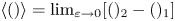 $\langle ()\rangle =\lim _{\varepsilon \to 0} [()_2-()_1]$ represents the change in the indicated property across a shock. Although our model does not show a typical shock, we can still quantitatively estimate the change in
  $q$ by applying (3.6) to the region containing the hydraulic transition. From model output, we estimate
  $\langle B \rangle$ and
  $\langle q \rangle$ from the differences between a downstream section
  $y=40$ and the sill
  $y=35$ (‘
 $\times$’ symbols in figure 11d,e), and between the sill and a upstream section
  $y=30$ (‘
 $+$’ symbols), respectively. Over
  $35\leq y\leq 40$,
  $\langle B \rangle$ and
  $\langle q \rangle$ both show a large magnitude at larger
  $\varPsi$, which corresponds to streamlines near the eastern edge of the flow;
  $\langle q \rangle$ calculated from (3.6) overestimates but agrees with the order of magnitude of change (lower solid curve in figure 11d). On the contrary,
  $\langle q \rangle$ computed over
  $30\leq y\leq 35$ and predicted from theory (upper solid curve in figure 11d) are both near zero. This further confirms the existence of a dissipative hydraulic transition downstream of the sill, across which the potential vorticity decreases. Since the friction model contains no explicit friction in this region, the dissipation must arise from implicit dissipation due to the numerical scheme. The same is true for in past simulations using the same model, e.g. Pratt et al. (Reference Pratt, Helfrich and Chassignet2000).
(a–c) Flow thickness  $d$, potential vorticity
  $q$ and Bernoulli function
  $B$ at the southern boundary of the model domain
  $y=0$ (dotted curves), the upstream channel entrance at
  $y=30$ (solid black curves), the sill at
  $y=35$ (grey thick curves) and a downstream section at
  $y=40$ (dashed black curves). Triangles and circles mark locations of streamlines
  $\varPsi =-0.46$ (thick dashed curves in figure 10a,b) and
  $\varPsi =-0.3$ (thick solid curves in figure 10a,b), respectively. (d,e) Along-streamline change in
  $q$ and
  $B$ between the sill and the upstream section (‘
 $+$’ symbols) and between the downstream section and the sill (‘
 $\times$’ symbols), respectively. Results are from the time-averaged friction model output for topographic parameters (
 $r_s=1.3$,
  $h_s=0.6$), except that the solid curves in (d) are predictions from shock theory.

3.4. The hydraulics of splitting flow
The circulation integral (1.1) expresses the need for friction to act on the east side of the island in order to support a steady, hydraulically controlled flow in the channel. We now return to the steady form of this integral as it applies in the numerical model
 \begin{equation} \oint_{C_l}(f+\zeta)\boldsymbol{u}\boldsymbol{\cdot}\boldsymbol{n}\,\mathrm{d}s =\delta{B}-\oint_{C_l}\lambda\boldsymbol{u}\boldsymbol{\cdot}\boldsymbol{l}\,\mathrm{d}s, \end{equation}
and contrast the various terms and balances that arise in the friction and no-friction experiments. In both model settings, the island topography varies smoothly. Therefore, at the edge of the flow, the layer thickness vanishes and values of velocity are particularly susceptible to numerical noise. With this in mind, we have opted to consider an alternative contour  $C_l$ that lies slightly offshore of the island where the layer depth is finite and noise is a minor issue. The constructed
  $C_l$ consists of a streamline that coincides with the eastern edge of the flow in the channel
  $S_4$, a streamline around the island
  $S_2$, a meridional segment
  $S_1$ and a zonal segment
  $S_3$ that connect
  $S_2$ and
  $S_4$ at the entrance and downstream of the channel, respectively (figure 12a). The transport streamfunction and all the variables in (3.7) are computed from the friction model output averaged over
  $100\leq t\leq 800$. The Rayleigh friction coefficient
  $\lambda$ was set to zero within the channel and 0.2 at
  $x>15$ for the friction experiments, therefore the integrations of the friction term along
  $S_1$ and
  $S_4$ are both zero. Equation (3.7) can then be re-written as
 \begin{equation} -\int_{S_1}q(ud)\,\mathrm{d} y+\int_{S_3}q(vd)\,\mathrm{d}\kern0.7pt x =\delta{B}-\int_{S_2}\lambda\boldsymbol{u}\boldsymbol{\cdot}\boldsymbol{l}\,\mathrm{d}s+\int_{S_3}\lambda u\,\mathrm{d}\kern0.7pt x. \end{equation}
(a) An example of an integration contour for Kelvin's circulation theorem analysis:  $S_1$ along
  $x=2.1$,
  $S_2$ the streamline of
  $\varPsi =-0.1$,
  $S_3$ along
  $y=45.9$ and
  $S_4$ the streamline of
  $\varPsi =-0.3$. (b) Terms of the simplified Kelvin circulation theorem for a steady flow as expressed in (3.8). Results are calculated from different choices of integration circuits and shown with black vertical lines as
  $\pm$ one standard deviation about the mean. Also shown are the sum of terms on the left-hand side (LH) of (3.8), the sum of the right-hand side (RH) terms and the difference between the two terms (LH-RH). (a) and (b) are both from the time-averaged friction model output. (c) Same as in (b) but for the terms calculated from the no-friction model output averages. Topographic parameters for both experiments are (
 $r_s=1.3$,
  $h_s=0.6$).

We calculate the terms in (3.8) using several, slightly different, choices of the integration contour;  $S_2$ and
  $S_4$ are defined to coincide with
  $\varPsi$ ranging from
  $-$0.1 to
  $-$0.02 and
  $-$0.38 to
  $-$0.24, respectively;
  $S_1$ and
  $S_3$ are chosen to lie in the range of
  $1\leq x\leq 3$ and
  $44\leq y\leq 50$, respectively. Bringing together the terms in (3.8) calculated from all the choices of integration circuits shows that the left and right sides of the equation are nearly balanced (figure 12b). In particular, the positive Bernoulli difference between upstream and downstream of the hydraulic transition is primarily balanced by the negative bottom friction integral.
For comparison, we compute the transport streamfunction from the time-averaged no-friction numerical model results and calculate all the terms in (3.8) (figure 12c). Choices for the integration contour are the same as for the friction model results, except that we restrict  $S_4$ to a more limited range of
  $\varPsi$,
  $-$0.38 to
  $-$0.32 due to the large noise near the eastern edge of the flow. For the no-friction experiments, the frictional dissipation term is exactly zero. The gain of potential vorticity is also very close to zero with very small variance. A positive time evolution term
 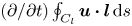 $({\partial }/{\partial t})\oint _{C_l}\boldsymbol {u}\boldsymbol {\cdot }\boldsymbol {l}\,\mathrm {d}s$ is needed to balance the small but positive
  $\delta {B}$, which explains the accelerating counter-clockwise circulation around the island shown in figure 6(e).
4. Samoan Passage
It has been revealed from recent observations that the Samoan Passage overflow is hydraulically controlled over a series of sills (Alford et al. Reference Alford, Girton, Voet, Carter, Mickett and Klymak2013), justifying the use of hydraulic theory to predict the partitioning of transport between the Samoan Passage and the eastern Manihiki Plateau.
As summarized in table 1, Whitehead (Reference Whitehead1998) treated the Samoan Passage as the only pathway of flow between two basins and neglected the existence of the path along the eastern flank of the Manihiki Plateau. The author used a ‘wide-channel’ assumption (i.e. a channel being much wider than the Rossby radius of deformation) and proposed a formula to estimate the transport of the controlled flow assuming zero potential vorticity (i.e. flow originated from an infinitely deep reservoir). A more detailed model from Girton et al. (Reference Girton2019) used the realistic cross-passage topography and considered a flow with non-zero potential vorticity. However, the model ignores flows around Manihiki Plateau and no critical condition is imposed, meaning that the estimated transport may not correspond to the hydraulically controlled flow and thus is smaller than other estimates from hydraulic theory. The model also requires considerable hydrographic measurements across the passage, which is not advantageous for long-term monitoring of transport. Pratt et al. (Reference Pratt, Voet, Pacini, Tan, Alford, Carter, Girton and Menemenlis2019) considered the pathway east of Manihiki and used an extended form of the Island Rule (Godfrey Reference Godfrey1989) to assess the transport partitioning of the northward deep western boundary current (DWBC). Although their formulation does not explicitly require nor lead to the presence of hydraulic control in the Samoan Passage, the transport prediction does rely on measurements of the turbulent dissipation there, a process that is amplified by hydraulic jumps downstream of the sills, and these exist only in the presence of hydraulic control. Moreover, their predicted transport depends upon, and is quite sensitive to, the value of the bottom drag coefficient around the island.
Volume transport through the Samoan Passage from different theories. PV stands for potential vorticity.

The theory we put forth in § 2 can also be employed to compute the hydraulically controlled transport in the Samoan Passage provided that the flow is of uniform potential vorticity and the cross-section topography can be simplified as a rectangle or a parabola. The excess transport of the northward DWBC is diverted east of the Manihiki Plateau and its value is obtained by subtracting the transport through the Samoan Passage from the total transport of the inflow. We particularly note that the flow in the Samoan Passage is hydraulically controlled whereas the branch to the east of the Manihiki Plateau is not, and the persisting hydraulic control in the Samoan Passage is accompanied by persisting turbulent mixing associated with hydraulic jumps downstream of the sills (Cusack et al. Reference Cusack, Voet, Alford, Girton, Carter, Pratt, Tan and Pearson-Potts2019). As detailed in § 3, friction along the eastern boundary of the plateau is required not only to support such a regime but also to support the decrease in Bernoulli function across the hydraulic transition of the controlled branch. Therefore, we consider for the Samoan Passage case the coastline of the Manihiki Plateau must be long enough, or the actual value of the friction coefficient must be large enough or both, for the existence of the persisting hydraulic control and the persisting hydraulic jump. The predicted division of transport from our theory does not depend on the values of the friction coefficient nor the size of the island, which is different from the model in Pratt et al. (Reference Pratt, Voet, Pacini, Tan, Alford, Carter, Girton and Menemenlis2019).
4.1. Samoan Passage transport from theory
In the non-dimensional version of our theory, the potential vorticity  $q$ and the upstream inflow volume flux
  $Q$ are upstream conditions required to estimate the critical transport through the channel
  ${Q_1}_c$. In the dimensionalized form, the potential depth
  $D_\infty$ serves as one upstream condition required for our theory. The interface of the Samoan Passage overflow is chosen to be the 1
  $^\circ$C isotherm, the most commonly accepted upper boundary of the DWBC in the Southern Pacific Ocean (Reid & Lonsdale Reference Reid and Lonsdale1974; Rudnick Reference Rudnick1997). Based on this,
  $D_\infty =1000$ m is determined according to the layer thickness below the 1
  $^\circ$C isotherm at the entrance to the passage (bottom depth
  $\sim$5200 m taken from figure 3 in Pratt et al. Reference Pratt, Voet, Pacini, Tan, Alford, Carter, Girton and Menemenlis2019 and figure 2 in Voet et al. Reference Voet, Girton, Alford, Carter, Klymak and Mickett2015). For the other upstream condition, we took the total transport below the 1.0
  $^{\circ }$C isotherm (
 $Q^*=9.9$ Sv) from Roemmich et al. (Reference Roemmich, Hautala and Rudnick1996) based on hydrographic measurements along a section crossing the Samoan Passage and the Manihiki Plateau. Note that we ignored the existence of the Robbie Ridge, which contains a transport of 1.1 Sv in Roemmich et al. (Reference Roemmich, Hautala and Rudnick1996), and assumed that the total transport of 9.9 Sv is partitioned between the Samoan Passage and east of the Manihiki Plateau. Values of
  $g'$ and
  $f$ are also required for the transport estimation, which are taken from Girton et al. (Reference Girton2019) (
 $4\times 10^{-4}$ m s
 $^{-2}$) and estimated at 8
  $^\circ$S (
 $2\times 10^{-5}$ s
 $^{-1}$), respectively. Given a generic depth scaling in the channel
  $D=1000$ m yields
  $L_d\approx 31$ km and dimensionless upstream conditions
  $q=-1$ and
  $Q\approx 0.5$. Note that the resulting
  ${Q^*_1}_c$ in the dimensional form does not depend on the value of
  $D$.
$D$.
Additional to upstream conditions, geometric parameters of the critical section are needed to estimate  ${Q^*_1}_c$. Here, we assume that the critical section lies at the sill according to the inviscid hydraulic theory. Observations have shown that the transport in the Samoan Passage splits into two major pathways, each with multiple contractions and sills (Voet et al. Reference Voet, Girton, Alford, Carter, Klymak and Mickett2015; Girton et al. Reference Girton2019). From a visual inspection of figure 3 in Girton et al. (Reference Girton2019), the 1.0
  $^{\circ }$C isotherm is located near 4000 m and spans over a distance of approximately 20 and 40 km at the western path sill (P2) and the eastern path sill (P4), respectively (also see in figure 1c,d). The two sills are approximately 600 and 400 m above the sea bottom depth at the entrance to the Samoan Passage. When determining the topographic parameters representing the Samoan Passage, we treated the two pathways as one channel with a sill height of 600 m and a width of 50 km, and further assumed that the contraction in the channel width is located at the sill. Values of
  $h^*_c=600$ m and
  $w^*_c=50$ km are considered as geometric parameters at the critical section and used in estimating the overflow transport from theory. Non-dimensional versions are
  $h_c=0.6$ and
  $w_c\approx 1.6$, respectively. For comparison, we also estimated the transport partitioning for the narrow- and shallow-channel limit (
 $h_c=0.6$,
  $w_c=0.6$) and the wide- and deep-channel limit (
 $h_c=0.4$,
  $w_c=1.6$). Considering that our estimate of the local geometry is rather subjective, the range of estimates can be seen as an uncertainty estimate to some extent. We then fit the Samoan Passage to a parabola by assuming
  $w^*_c$ to be the width of the overflow interface and
  $d^*_c=500$ m to be the thickness of flow between the deepest point of the parabola and the interface. The latter value is taken from figure 3 in Girton et al. (Reference Girton2019). The curvature parameter is
  $\alpha \approx 8\times 10^{-7}$ m
 $^{-1}$, or in the non-dimensional form
  $r_c\approx 1.3$, and the non-dimensional sill height at the bottom of the parabola is
  ${h_0}_c=0.6$. The two limits for sensitivity test are (
 ${h_0}_c=0.6$,
  $r_c=0.2$) and (
 ${h_0}_c=0.4$,
  $r_c=1.3$), respectively.
Our theory for a rectangular channel yields a transport in the Samoan Passage of  ${Q^*_1}_c=7.4$ Sv (
 ${Q_1}_c\approx 0.38$), and the sensitivity test yields transports of 4.3 and 10.2 Sv (
 ${Q_1}_c\approx 0.22$ and 0.52) for geometric parameters under narrow-channel limit and wide-channel limit, respectively. To compare, the parabolic channel formulation predicts
  ${Q^*_1}_c=6.0$ Sv (
 ${Q_1}_c\approx 0.3$), and results from the sensitivity test are
  ${Q^*_1}_c=3.3$ and 8.5 Sv (
 ${Q_1}_c\approx 0.17$ and 0.43). Transports estimated from the parabolic channel theory are smaller than the estimates for a rectangular channel. As shown in figures 3 and 4(a), except for the wide-channel limit, our selected topographic parameters are within the regime of a hydraulically controlled flow. Overall, the theory-based transport estimates lie reasonably close to the time-mean estimates of 5.4 Sv (Voet et al. Reference Voet, Alford, Girton, Carter, Mickett and Klymak2016) and 6.0 Sv (Rudnick Reference Rudnick1997) obtained from moored measurements.
4.2. Two major pathways of flow in the Samoan Passage
Let us now consider a case where there are two narrow parabolic channels to the west of the island, which is a more realistic representation for the Samoan Passage. The western channel is narrower and shallower at the sill ( $w_W^*=20$ km,
  ${h_0}_W^*=600$ m) and the eastern channel (note the difference from the ‘eastern passage’, which refers to the vast passage to the east of the island; the ‘eastern channel’ is part of the Samoan Passage and thus is narrow) is wider and deeper at the sill (
 $w_E^*=40$ km,
  ${h_0}_E^*=400$ m) (figure 13a,e). Dimensionless topographic parameters for the two channels are (
 $r_W\approx 0.18$,
  ${h_0}_W=0.6$) and (
 $r_E\approx 0.72$,
  ${h_0}_E=0.4$), respectively. Whitehead (Reference Whitehead2003) proposed an analytical solution to the partitioning of inflow among multiple channels by assuming such a scenario that the meridional inflow tends to pass through the westernmost channel, where the hydraulic control is preferentially established. The residuals of the inflow, as a consequence, make their way to the second westernmost passage. If the flow in the second westernmost channel is also hydraulically controlled and the critical transport combined is less than the transport of the inflow, the residuals will enter the next passage to the east, and so on for the rest of the eastern passages. In other words, the hydraulic control in a western channel is independent of processes within the passages to its east. This scenario has been adopted by Girton et al. (Reference Girton2019) to estimate the transport through the Samoan Passage, although many historical numerical simulations (e.g. Helfrich & Pratt Reference Helfrich and Pratt2003) as well as ours suggest that, even when the inflow approaches along the western wall, it veers offshore and enters the channel from the eastern side, which is due to the topographic beta effect.
Numerical results from the friction experiments but with two channels. (a) Magnified view of the northward velocity  $v$ (colour) and the interface height
  $d+h$ (contours) in the channel at
  $t=400$. Panels (b) and (c) show the predicted transport (solid curves) and transport calculated from numerical simulations (dots) given different widths and sill heights of the eastern channel, while keeping other topographic parameters unchanged. Panels (a,d,e) are from the same model topographic parameters as indicated above (d). (d) Time series for the transport of the inflow
  $Q$, total transport of the two channels
  $Q_{1W}+Q_{1E}$, transport in the western channel
  $Q_{1W}$, transport in the eastern channel
  $Q_{1E}$ and transport along the eastern flank of the island
  $Q_2$. Numerical results and analytical solutions for the critical transport are shown in solid lines and dashed lines, respectively. (e) Values of
  $v$ and
  $d+h$ at the sill (grey line in (a)). Red vectors and curves are analytical solutions from the theory. Blue vectors and areas are results from numerical runs averaged over
  $t=100\text{--} 400$.

Despite these flaws, here we give an estimate of transport in the two channels within the Samoan Passage based on Whitehead (Reference Whitehead2003). We then compare the results with the transport computed from the numerical simulations to evaluate the validity of the theory. To implement the theory, first we compute the controlled transport in the western channel using upstream conditions and the topographic features of the sill. Then we compute the Bernoulli function along the eastern boundary of the western channel, which would be the same as the Bernoulli function along the western boundary of the eastern channel in the scenario suggested by Whitehead (Reference Whitehead2003). The along-boundary Bernoulli function combined with sill topography provides enough information to compute the critical transport of the eastern channel. Using this methodology, we compute a series of critical transports in the two channels by changing the width (figure 13b) or height (figure 13c) of the eastern channel while keeping other topographic parameters unchanged.
Theory predicts transports of  ${Q_{1W}}_c\approx 0.17$ and
  ${Q_{1E}}_c\approx 0.28$, or dimensionally, 3.3 Sv and 5.6 Sv for the western channel and eastern channel in the Samoan Passage, respectively. However, numerical results are both smaller than the theory predictions (
 ${Q_{1W}}\approx 0.13$,
  ${Q_{1E}}\approx 0.26$; or dimensionally, 2.5 and 5.0 Sv), especially for the transport in the western channel. By changing the topography of the eastern channel while leaving the western channel unchanged, we find the difference between model results and theoretical predictions is most evident when the eastern channel is wide and deep. Both theory and model assume inviscid flow in the two channels, which allows frontal waves to propagate along the boundary of the separation land of the two channels and connect the two channels. In this case, the western channel is not independent from processes in the eastern channel. However, since the mismatch between the theory and model is reasonably small, especially when the eastern channel is of modest width and height, one may still use the theory to estimate the transport.
5. Summary
This work has examined the hydraulics of a flow passing between ocean basins through a twin passage, one narrow and containing a topographic sill, and the other broad, using shallow-water theory and numerical simulations. We regard the Samoan Passage and the Manihiki Plateau system in the Southern Hemisphere as a prototype, where the northward-flowing DWBC splits into two flows: one entering the Samoan Passage and being hydraulically controlled by topography, the other passing to the east of Manihiki as a boundary current that is likely not controlled. Our problem is different from historical models such as Whitehead, Leetmaa & Knox (Reference Whitehead, Leetmaa and Knox1974) and Gill (Reference Gill1977), which considered two basins connected by a single channel, in that upstream disturbances such as Kelvin/frontal waves initiated at the critical section do not propagate back into the upstream basin and therefore do not exert any upstream influence. Those waves instead propagate along the boundary of the island eventually arriving downstream, a feature that makes it possible to specify the upstream transport independently of the characteristics of the sill.
In § 2, we propose formulae for both rectangular and parabolic channel cross-sections that connect properties (potential vorticity and transport) of the upstream inflow (DWBC) and the geometry of the sill (height and width) with the transport of the hydraulically controlled flow in the channel. The channel flow is choked by topography, meaning that not all the upstream transport can enter the channel. Had there been only one passage, hydraulic adjustment would occur in the upstream basin as well as in the channel (Pratt et al. Reference Pratt, Helfrich and Chassignet2000). In our case, the excess transport is carried by a boundary current that flows along the eastern boundary of the island and joins the channel outflow in the downstream basin. As long as the formulae successfully predict the critical transport in the Samoan Passage, we can then simply subtract that transport from the total transport of the DWBC to determine the transport to the east of Manihiki.
The fact that the Kelvin/frontal waves initiated upstream of the sill propagate along the eastern boundary of the island instead of entering the upstream basin (i.e. no upstream influence) raises the question of how the hydraulically controlled flow in the channel can persist under the condition that those waves may eventually go around the island and enter the channel from downstream. To answer this question, we employed a numerical model and found that a steady-state hydraulic control of an inviscid channel flow is only possible if some frictional drag has been added to the east of the island (friction experiments in § 3). From the model output, we found that the lowest frontal wave modes trapped to the east edge of the channel flow undergo a transition from supercritical to subcritical downstream of the sill. Flow characteristics within the region of the hydraulic transition from our simulations are particularly of interest since the channel in our model has rounded topographic cross-sections and the channel flow has no upstream influence due to our model set-up, which differs from other historical numerical models with vertical walls that have a single channel. Following a streamline passing through the channel, both Bernoulli function and potential vorticity decrease across the hydraulic transition. This non-conservation shows asymmetry in the cross-channel direction with a larger change near the east edge of the flow than the west edge of the flow. Moreover, the declines are gradual and the flow does not reveal features of a rotating shock nor a transverse hydraulic jump as produced by historical numerical models with vertical walls (e.g. Pratt Reference Pratt1983, Reference Pratt1987; Pratt et al. Reference Pratt, Helfrich and Chassignet2000, Reference Pratt, Riemenschneider and Helfrich2007). By examining the terms in the equation for the Kelvin circulation theorem, we found that the decrease in Bernoulli function must be balanced by the frictional energy dissipation in the flow to the east of the island, or the flow that encircles the island will accelerate and no steady state can be achieved. The latter is the case in the no-friction experiments in § 3, where circum-island frontal waves intrude into the channel from downstream and the flow becomes subcritical everywhere and there is thus a lack of control.
We also examined cases in which the passage between the island and the western boundary consists of two separate channels. It is possible to predict the distribution of transports in the two channels by assuming that both are hydraulically controlled and that conditions in the eastern channel do not affect those in the western channel. Transports estimated based on these assumptions agree with numerical results to within 10 % when the width of the eastern channel is small or when the height of the eastern channel sill is tall ( $r_{E}\leq 0.5$,
  ${h_0}_E\geq 0.4$).
Acknowledgements
S.T. gratefully acknowledges the support of the Chinese Scholarship Council during her visit at Woods Hole Oceanographic Institute. The work has benefited from critical readings by A. Saberi and discussions with D. Yuan. We also thank three anonymous reviewers for their valuable comments.
Funding
This work was supported by the National Science Foundation under grants OCE-1029268, OCE-1029483, OCE-1657264, OCE-1657795, OCE-1657870 and OCE-1658027.
Declaration of interests
The authors report no conflict of interest.
Author contributions
The first author was primarily responsible for the development of the theory, all of the computations and most of the writing of the manuscript, although considerable input was provided by the second author. The work was initiated three years ago and all eight authors contributed to its development as part of regular discussions that took place as the work unfolded. All eight co-authors have read drafts of the manuscripts.
Data availability statement
Codes that solve the hydraulic theory and make all plots are openly available at the repository (https://github.com/ShuwenTan-PO/GillModel). Contact S.T. for codes and output files for the numerical model.
Appendix A. Wave mode calculation
Flow properties ( $u, v, d$) may be separated into a background steady state (
 $U, V, D$) and a perturbation (
 $u', v', d'$). The shallow-water equations can then be linearized to obtain the linear equations of perturbations. A one-directional wave-like perturbation may take the form
 \begin{equation} \phi'(x,y,t)=Re[\hat{\phi}(x)\,{\rm e}^{{\rm i}l(y-ct)}], \end{equation}
where  $\phi '$ represents a perturbation of any flow property,
  $\hat {\phi }$ is a complex,
  $x$-dependent eigenfunction,
  $c$ is a complex phase speed and
  $l$ is the wavenumber in the
  $y$-direction.
The problem can be further simplified by assuming a parallel background flow of  $U=0$,
  $V=V(x)$ and
  $D=D(x)$, and the linear equations of perturbations then yield (derived from (3.1)–(3.3))
 \begin{equation} \left. \begin{array}{c@{}}
\sigma\hat{u}={-}\left({\rm
i}lV-\nu\dfrac{\partial^2}{\partial x^2}+\nu
l^2\right)\hat{u} +{\rm
sign}(f)\hat{v}-\dfrac{\partial}{\partial x}\hat{d},\\
\sigma\hat{v}={-}(V_x+{\rm sign}(f))\hat{u}-\left({\rm
i}lV-\nu\dfrac{\partial^2}{\partial x^2}+\nu
l^2\right)\hat{v}-{\rm i}l\hat{d},\\
\sigma\hat{d}={-}\left(D\dfrac{\partial}{\partial
x}+D_x\right)\hat{u}-{\rm i}lD\hat{v}-{\rm i}lV\hat{d},
\end{array}\right\} \end{equation}
\begin{equation} \left. \begin{array}{c@{}}
\sigma\hat{u}={-}\left({\rm
i}lV-\nu\dfrac{\partial^2}{\partial x^2}+\nu
l^2\right)\hat{u} +{\rm
sign}(f)\hat{v}-\dfrac{\partial}{\partial x}\hat{d},\\
\sigma\hat{v}={-}(V_x+{\rm sign}(f))\hat{u}-\left({\rm
i}lV-\nu\dfrac{\partial^2}{\partial x^2}+\nu
l^2\right)\hat{v}-{\rm i}l\hat{d},\\
\sigma\hat{d}={-}\left(D\dfrac{\partial}{\partial
x}+D_x\right)\hat{u}-{\rm i}lD\hat{v}-{\rm i}lV\hat{d},
\end{array}\right\} \end{equation}
where  $\sigma =-\textrm {i}lc$ is the growth rate. Since we focus on the flow through the channel,
  $\lambda$ is not present in (A2). For a parallel,
  $x$-dependent background flow, the form drag introduced by the varying topography in the
  $y$-direction must be balanced by the viscous force. So it is reasonable to include a small viscosity
  $\nu$ in (A2), although the numerical model may not contain any frictional terms. A small viscous term also helps to smooth out the wave modes with many wiggles (e.g. singular modes that are discontinuous in
  $x$, underresolved modes that have a large wavenumber, etc.). Here,
  $\nu =10^{-7}$ is used to compute the wave modes, for it is large enough to result in some smooth modes and also small enough to give results similar to those computed from the inviscid equations;
  $l$ is set to
  $10^{-6}$ since the long waves are prone to being non-dispersive and the most relevant to the flow hydraulics. The boundary conditions at the free edges are
 $$\begin{gather} D\hat{u}=0, \end{gather}$$
 $$\begin{gather}D\nu\frac{\partial \hat{u}}{\partial x}=0, \end{gather}$$
which are automatically satisfied for finite values of velocity and viscous momentum flux at free edges since  $D=0$ there.
The matrix eigenvalue equations (A2) are solved numerically using the cross-channel profiles of  $V$ and
  $D$ at locations between
  $y=30$ and
  $y=40$ from the numerical simulations. From the many wave mode solutions, the Poincaré waves (or mixed potential vorticity–gravity waves) can be easily identified by their extremely large phase speeds/very high frequency and the undulating
  $\hat {u}$ with amplitudes larger than those of
  $\hat {v}$ and
  $\hat {d}$. Most of these modes are highly unstable. However, it is the frontal waves whose speeds are comparable to the flow speed that are most relevant to the hydraulic behaviours. We therefore exclude the Poincaré wave modes that have a large
  $\hat {u}$ and sort the rest of the modes by phase speed. The lowest and the second-lowest mode pairs are featured with none (0
 $^{th}$ mode) and one zero crossings (1th mode), respectively. We find that most of these modes (and almost all for the 0th modes) have phase speeds lying outside of the range of
  $V(x)$. The amplitude of the 0th modes peaks near and decays from the edges of the flow, which confirms that the modes we selected are frontal waves that have similar decaying features as Kelvin waves.


 Open access