





1. Introduction
Solute transport in fractured rock networks plays a central role in a wide range of subsurface applications (Berkowitz Reference Berkowitz2002), including carbon sequestration (Szulczewski et al. Reference Szulczewski, MacMinn, Herzog and Juanes2012), nuclear waste storage (Tsang et al. Reference Tsang, Birkholzer and Rutqvist2015) and geothermal energy extraction (Ren et al. Reference Ren, Kong, Pang and Wang2023). Fractured media, such as that shown in figure 1(a), constitute a particular class of porous material characterised by networks of high-permeability fractures embedded within a comparatively low-permeability rock matrix (Berre, Doster & Keilegavlen Reference Berre, Doster and Keilegavlen2019). These fractures often possess large aspect ratios and arise through a variety of geological processes including tectonic deformation (Bonnet et al. Reference Bonnet, Bour, Odling, Davy, Main, Cowie and Berkowitz2001), thermo-mechanical stresses (Safari & Ghassemi Reference Safari and Ghassemi2015) and biological activity in the subsurface (Stembridge Reference Stembridge1978). Although mixing within fracture systems exerts a first-order control on many fluid-borne processes, including solute dilution (Zhao, Li & Jiang Reference Zhao, Li and Jiang2014), geochemical reactions (Lee, Yoon & Kang Reference Lee, Yoon and Kang2023) and biological activity (Bochet et al. Reference Bochet2020; Schuler et al. Reference Schuler2024), flow through fracture networks can generate complex mixing dynamics that are not fully understood (Hyman & Jiménez-Martínez Reference Hyman and Jiménez-Martínez2018; Hallack et al. Reference Hallack, Bolster, Hyman, Sweeney and Viswanathan2025).
Fracture networks consist of finite-sized three-dimensional (3-D) intersecting fractures, often with large aspect ratios. Denoting the characteristic fracture aperture by $\ell$
and the fracture width by
$\ell$
and the fracture width by $L$
, these systems satisfy
$L$
, these systems satisfy $\ell \ll L$
. Consequently, flow and transport within individual fractures appear effectively two-dimensional (2-D) at the fracture scale
$\ell \ll L$
. Consequently, flow and transport within individual fractures appear effectively two-dimensional (2-D) at the fracture scale $L$
, while remaining intrinsically 3-D at the aperture scale
$L$
, while remaining intrinsically 3-D at the aperture scale $\ell$
. The narrow geometry of fracture apertures typically renders inertial effects generally negligible, such that the flow is Stokesian at the aperture scale
$\ell$
. The narrow geometry of fracture apertures typically renders inertial effects generally negligible, such that the flow is Stokesian at the aperture scale $\ell$
and can often be approximated by Darcy flow at the fracture scale
$\ell$
and can often be approximated by Darcy flow at the fracture scale $L$
.
$L$
.
These geometric considerations motivate the widely used discrete fracture network (DFN) framework, in which fracture systems are represented as a complex of 2-D fracture planes connected by one-dimensional (1-D) intersections embedded within a 3-D matrix (figure 1 b) (Jing & Stephansson Reference Jing and Stephansson2007). In this approach, Darcy flow equations are solved on the fracture surfaces with coupling through the intersections, yielding a computationally tractable representation of flow and transport. Considerable progress has recently been made in understanding solute dispersion within such DFN models (Hyman et al. Reference Hyman, Painter, Viswanathan, Makedonska and Karra2015; Hyman Reference Hyman2020; Hyman et al. Reference Hyman, Sweeney, Gable, Svyatsky, Lipnikov and Moulton2022; Dentz & Hyman Reference Dentz and Hyman2023; Davy et al. Reference Davy, Le Goc, Darcel, Pinier, Selroos and Le Borgne2024). However, an outstanding challenge is to understand and predict mixing dynamics within fracture networks (figure 2).
(a) Fractured rock in Cape Otway, Victoria, Australia, with fractures indicated by superimposed red lines and intersections as green dots. Orange bands around fractures indicate regions of chemical activity. (b) Oblique view of a simple DFN comprising $N_F=5$
fractures labelled
$N_F=5$
fractures labelled $F_n$
(
$F_n$
( $n=1:N_F$
) and
$n=1:N_F$
) and $N_I=8$
intersections labelled
$N_I=8$
intersections labelled $I_m$
, (
$I_m$
, ( $m=1:N_I)$
(green lines). Inlet fractures
$m=1:N_I)$
(green lines). Inlet fractures $F_2$
and
$F_2$
and $F_4$
, and outlet fractures
$F_4$
, and outlet fractures $F_3$
and
$F_3$
and $F_5$
terminate at and intersect with the central fracture
$F_5$
terminate at and intersect with the central fracture $F_1$
. Streamlines are coloured red or blue respectively depending upon whether they enter via
$F_1$
. Streamlines are coloured red or blue respectively depending upon whether they enter via $F_2$
or
$F_2$
or $F_4$
(as indicated by coloured arrows) and are routed through
$F_4$
(as indicated by coloured arrows) and are routed through $F_1$
before exiting via
$F_1$
before exiting via $F_3$
or
$F_3$
or $F_5$
(as indicated by coloured arrows). (c) Plan view of streamline topology in fracture
$F_5$
(as indicated by coloured arrows). (c) Plan view of streamline topology in fracture $F_1$
in panel (b), indicating routing from ‘source’ intersections
$F_1$
in panel (b), indicating routing from ‘source’ intersections $I_1$
,
$I_1$
, $I_3$
(green lines) to ‘sink’ intersections
$I_3$
(green lines) to ‘sink’ intersections $I_2$
,
$I_2$
, $I_4$
(green lines) via separating streamlines (black lines) and critical points (black points). Red and blue arrows respectively indicate unstable and stable manifolds. Symbol
$I_4$
(green lines) via separating streamlines (black lines) and critical points (black points). Red and blue arrows respectively indicate unstable and stable manifolds. Symbol $\psi _1$
denotes direction of increasing
$\psi _1$
denotes direction of increasing $\psi _1$
– streamfunction
$\psi _1$
– streamfunction $\psi _1$
– along an intersection.
$\psi _1$
– along an intersection.

Advective mixing in fracture networks (computed via DFN.lab) comprising fractures $F_n$
and faces
$F_n$
and faces $f_n$
(defined in § 3.1 as 2-D cross-sections of 3-D fractures at their boundary) that exhibit (a, b) fracture mixing only and (c, d) intersection mixing only. (a) Fracture mixing arising from red and blue streamlines entering inlet faces
$f_n$
(defined in § 3.1 as 2-D cross-sections of 3-D fractures at their boundary) that exhibit (a, b) fracture mixing only and (c, d) intersection mixing only. (a) Fracture mixing arising from red and blue streamlines entering inlet faces $f_1$
and
$f_1$
and $f_2$
. There streamlines are interleaved as ‘parcels’ that exit at outlet faces
$f_2$
. There streamlines are interleaved as ‘parcels’ that exit at outlet faces $f_3$
and
$f_3$
and $f_4$
, resulting in large-scale fracture mixing. (b) Mapping of inlet concentration field in faces
$f_4$
, resulting in large-scale fracture mixing. (b) Mapping of inlet concentration field in faces $f_1$
and
$f_1$
and $f_2$
to
$f_2$
to $f_3$
and
$f_3$
and $f_4$
via the fracture mixing map
$f_4$
via the fracture mixing map ${\mathcal{M}_F}$
(3.10) corresponding to the fracture mixing shown in panel (a) in terms of local streamfunctions
${\mathcal{M}_F}$
(3.10) corresponding to the fracture mixing shown in panel (a) in terms of local streamfunctions $(\psi _{1,n},\psi _{2,n})$
,
$(\psi _{1,n},\psi _{2,n})$
, $n=1:4$
(defined in § 3.1) at face
$n=1:4$
(defined in § 3.1) at face $f_n$
. (c) Intersection mixing arising from streamline routing at intersections. Red and blue streamlines entering inlet faces
$f_n$
. (c) Intersection mixing arising from streamline routing at intersections. Red and blue streamlines entering inlet faces $f_1$
and
$f_1$
and $f_2$
are finely interleaved before exiting at outlet faces
$f_2$
are finely interleaved before exiting at outlet faces $f_3$
and
$f_3$
and $f_4$
, resulting in fine-scale intersection mixing. (d) Mapping of inlet concentration field in faces
$f_4$
, resulting in fine-scale intersection mixing. (d) Mapping of inlet concentration field in faces $f_1$
and
$f_1$
and $f_2$
to
$f_2$
to $f_3$
and
$f_3$
and $f_4$
via the intersection mixing map
$f_4$
via the intersection mixing map ${\mathcal{M}_I}$
(3.9) corresponding to the intersection mixing shown in panel (c) in terms of local streamfunctions
${\mathcal{M}_I}$
(3.9) corresponding to the intersection mixing shown in panel (c) in terms of local streamfunctions $(\psi _{1,n},\psi _{2,n})$
at face
$(\psi _{1,n},\psi _{2,n})$
at face $f_n$
.
$f_n$
.

Although mixing of diffusive species such as solutes and colloids is of direct practical importance, these processes cannot be properly understood without first resolving the underlying advective dynamics (Metcalfe, Lester & Trefry Reference Metcalfe, Lester and Trefry2023). Advective mixing – comprising the stretching, folding, cutting and rearrangement of fluid elements – provides the kinematic foundation upon which diffusion, colloidal transport, chemical reactions and biological processes act (Zhao et al. Reference Zhao, Li and Jiang2014; Lee et al. Reference Lee, Yoon and Kang2023; Schuler et al. Reference Schuler2024). Quantitative prediction of these processes therefore requires a detailed understanding of the advective drivers of mixing. In the dynamical systems literature, fluid stirring is often referred to simply as mixing (Arnold & Avez Reference Arnold and Avez1968), whereas in the physical sciences, mixing typically denotes the combined action of advection and diffusion (Villermaux Reference Villermaux2019). Here we distinguish advective mixing, arising purely from fluid deformation, from solute mixing, which results from the combined effects of advection and diffusion. Despite recent progress, the fundamental mechanisms governing advective mixing in fracture networks remain poorly understood.
This gap is reflected in the substantial body of work examining solute mixing at fracture intersections (Berkowitz, Naumann & Smith Reference Berkowitz, Naumann and Smith1994; Park et al. Reference Park, de Dreuzy, Lee and Berkowitz2001; Li Reference Li2002; Hyman & Jiménez-Martínez Reference Hyman and Jiménez-Martínez2018; Sherman et al. Reference Sherman, Hyman, Bolster, Makedonska and Srinivasan2019). Many existing models represent mixing at intersections through flux-weighted random streamline routing, which effectively assumes instantaneous mixing and corresponds to a vanishing Péclet number. Such approaches cannot readily be generalised to finite Péclet numbers, and are incompatible with the deterministic and reversible nature of advective transport. Furthermore, because DFN models represent fractures as 2-D surfaces connected by 1-D intersections, transverse concentration profiles across the fracture aperture cannot be resolved. These limitations hinder development of analytic models of solute mixing in fracture networks and identification of the network properties that govern mixing.
A central question therefore concerns the extent to which dimensional reduction in DFN models constrains the admissible mixing dynamics. Recent work has begun to quantify mixing metrics such as the growth rate of material interfaces in DFNs (Hallack et al. Reference Hallack, Bolster, Hyman, Sweeney and Viswanathan2025), yet the underlying mechanisms remain unclear. In particular, because the flow within DFN models is restricted to 2-D fracture planes, the resulting steady flows must be non-chaotic according to the Poincaré–Bendixson theorem (Katok & Hasselblatt Reference Katok and Hasselblatt1995) (despite the 2-D fractures being embedded in a 3-D matrix). This restriction leads to characteristic non-chaotic mixing signatures, such as the algebraic growth of material interfaces observed in recent studies (Hallack et al. Reference Hallack, Bolster, Hyman, Sweeney and Viswanathan2025). Although it is recognised that topological complexity can generate chaotic advection under steady flow in pore networks and granular matter Lester et al. (Reference Lester, Heyman, Méheust and Le Borgne2025a ), it is unclear to what extent these dynamics are hindered by the constrained geometry inherent to fracture networks.
While parsimonious representations of transport, mixing and reactions in fracture networks are essential for large-scale modelling, properly resolving these 3-D mixing mechanisms is equally important. Representing fractures as strictly 2-D objects constrains the admissible Lagrangian kinematics, suppresses the influence of fracture roughness on transport and mixing, and may eliminate key processes such as fluid stretching and chaotic advection. Once these mixing mechanisms are resolved, it is then possible to develop faithful reduced-order representations of fluid-borne processes in fracture networks.
The aim of this study is therefore to elucidate and quantify the advective dynamics that govern mixing in 3-D DFNs in which fractures possess finite thickness. We consider the propensity for complex advective mixing dynamics such as chaotic advection and discontinuous mixing to arise in these networks, and develop an appropriate Lagrangian framework to represent advective mixing. Building on this understanding, we develop a highly accurate yet computationally efficient framework for modelling advective mixing in 3-D DFNs which is verified against numerical simulations performed using the open source code DFN.lab (Le Goc et al. Reference Le Goc, Pinier, Darcel, Lavoine, Doolaeghe, de Simone, De Dreuzy and Davy2019), https://fractorylab.org/dfnlab-software. Although DFN.lab is a 2-D DFN code, we show that via the use of a streamfunction coordinate system (the validity of which is established in § 2.3) that the 3-D flow field (in streamfunction coordinates) can be reconstructed from these 2-D simulations via local flux balances (see Appendix B). This proposed approach provides a basis for identification of the network properties that govern advective mixing, the development of quantitative mixing theories for large-scale networks, and facilitates the prediction of advection-mediated processes including solute dispersion, mixing and biogeochemical reactions in 3-D fracture networks. Similar to 2-D DFN models, the flow in 3-D DFNs is assumed to be steady and governed by isotropic Darcy flow throughout the fracture network. The implications of these assumptions are examined in § 2.1. The paper is structured as follows. In § 2, we develop a streamline coordinate system for advective mixing which is used to uncover the fundamental mixing mechanisms in 3-D DFNs. In § 3, we use the streamline coordinate system to construct a parsimonious representation of advective mixing in 3-D DFNs and in § 4, we verify this model against fully resolved DFN simulations. Conclusions and implications are discussed in § 5.
2. Advective mixing in fracture networks
2.1. Chaotic advection in fracture networks
To analyse advective mixing in fracture networks, we first consider the propensity for these systems to admit complex mixing dynamics and use this assessment to develop a parsimonious representation of advective mixing. We focus on fracture networks at negligible Reynolds number, $Re \ll 1$
, with large fracture aspect ratio
$Re \ll 1$
, with large fracture aspect ratio $\ell \ll L$
. Under these conditions, inertia-driven mixing mechanisms, such as those that arise at fracture intersections (Lee & Kang Reference Lee and Kang2020; Yang et al. Reference Yang, Chen, Lee and Kang2024), are absent. However, complex mixing dynamics may also arise in inertialess flows in topologically complex domains.
$\ell \ll L$
. Under these conditions, inertia-driven mixing mechanisms, such as those that arise at fracture intersections (Lee & Kang Reference Lee and Kang2020; Yang et al. Reference Yang, Chen, Lee and Kang2024), are absent. However, complex mixing dynamics may also arise in inertialess flows in topologically complex domains.
In the Stokes regime, steady flow in fracture networks may generate chaotic advection in a manner analogous to porous networks or granular media (Lester et al. Reference Lester, Metcalfe and Trefry2013, Reference Lester, Heyman, Méheust and Le Borgne2025a
). Pore and fracture networks both involve merging and branching of streamlines at pore junctions and fracture intersections, respectively, giving rise to localised stagnation points $\boldsymbol{x}_p$
, and associated unstable and stable 2-D hyperbolic manifolds; material surfaces that respectively undergo exponential stretching and contraction which are shown in figures 1(c), 3, 4, 5 and 7. If these manifolds intersect transversely, fluid elements undergo exponential stretching and folding, leading to chaotic advection (Ottino Reference Ottino1989). Indeed, several studies (Mourzenko et al. Reference Mourzenko, Yousefian, Kolbah, Thovert and Adler2002; Johnson, Brown & Stockman Reference Johnson, Brown and Stockman2006; Zhao et al. Reference Zhao, Li and Jiang2014) have examined steady 3-D Stokes flow in wide and rough fracture intersections, and found that although chaotic advection was not explicitly diagnosed, velocity fields were observed that exhibited 3-D structure consistent with non-trivial streamline braiding and thus chaotic advection (Boyland, Aref & Stremler Reference Boyland, Aref and Stremler2000). Conversely, tangential intersections between 2-D manifolds prohibit chaotic advection as the exponential expansion and contraction of hyperbolic manifolds exactly cancel. As fracture networks comprising narrow fractures impose strongly constrained geometries that favour near-tangential manifold intersections, the prevalence of chaotic advection under steady Stokes flow is unclear.
$\boldsymbol{x}_p$
, and associated unstable and stable 2-D hyperbolic manifolds; material surfaces that respectively undergo exponential stretching and contraction which are shown in figures 1(c), 3, 4, 5 and 7. If these manifolds intersect transversely, fluid elements undergo exponential stretching and folding, leading to chaotic advection (Ottino Reference Ottino1989). Indeed, several studies (Mourzenko et al. Reference Mourzenko, Yousefian, Kolbah, Thovert and Adler2002; Johnson, Brown & Stockman Reference Johnson, Brown and Stockman2006; Zhao et al. Reference Zhao, Li and Jiang2014) have examined steady 3-D Stokes flow in wide and rough fracture intersections, and found that although chaotic advection was not explicitly diagnosed, velocity fields were observed that exhibited 3-D structure consistent with non-trivial streamline braiding and thus chaotic advection (Boyland, Aref & Stremler Reference Boyland, Aref and Stremler2000). Conversely, tangential intersections between 2-D manifolds prohibit chaotic advection as the exponential expansion and contraction of hyperbolic manifolds exactly cancel. As fracture networks comprising narrow fractures impose strongly constrained geometries that favour near-tangential manifold intersections, the prevalence of chaotic advection under steady Stokes flow is unclear.
The common assumption of isotropic Darcy flow in 3-D DFNs further constrains the Lagrangian kinematics. Within fractures, steady 3-D Stokes flow may be validly approximated as a Hele-Shaw flow with variable aperture $h(\boldsymbol{x})\sim \ell$
across the fracture. Hence, for
$h(\boldsymbol{x})\sim \ell$
across the fracture. Hence, for $\ell \ll L$
, the flow in fractures can be validly approximated as an isotropic heterogeneous Darcy flow (Bear Reference Bear1972)
$\ell \ll L$
, the flow in fractures can be validly approximated as an isotropic heterogeneous Darcy flow (Bear Reference Bear1972)
 \begin{equation} \boldsymbol{v}(\boldsymbol{x})=-\frac {k(\boldsymbol{x})}{\mu }\boldsymbol{\nabla }p(\boldsymbol{x}), \end{equation}
where $\mu$
is the fluid viscosity and the permeability
$\mu$
is the fluid viscosity and the permeability $k(\boldsymbol{x})=h(\boldsymbol{x})^2/12$
. For 2-D and 3-D DFNs, it is assumed that isotropic Darcy flow extends throughout the entire fracture network. This renders the velocity field helicity-free (Sposito Reference Sposito2001; Lester et al. Reference Lester, Dentz, Bandopadhyay and Le Borgne2021), where from (2.1), the helicity density (Moffatt Reference Moffatt1969), defined as
$k(\boldsymbol{x})=h(\boldsymbol{x})^2/12$
. For 2-D and 3-D DFNs, it is assumed that isotropic Darcy flow extends throughout the entire fracture network. This renders the velocity field helicity-free (Sposito Reference Sposito2001; Lester et al. Reference Lester, Dentz, Bandopadhyay and Le Borgne2021), where from (2.1), the helicity density (Moffatt Reference Moffatt1969), defined as $\mathcal{H}(\boldsymbol{x}) \equiv \boldsymbol{v}\boldsymbol{\cdot }(\boldsymbol{\nabla }\times \boldsymbol{v})$
, vanishes identically as
$\mathcal{H}(\boldsymbol{x}) \equiv \boldsymbol{v}\boldsymbol{\cdot }(\boldsymbol{\nabla }\times \boldsymbol{v})$
, vanishes identically as
 \begin{equation} \mathcal{H}(\boldsymbol{x})\equiv \boldsymbol{v}(\boldsymbol{x})\boldsymbol{\cdot }(\boldsymbol{\nabla }\times \boldsymbol{v}(\boldsymbol{x}))=\frac {1}{\mu ^2}k(\boldsymbol{x})\boldsymbol{\nabla }p(\boldsymbol{x})\boldsymbol{\cdot }(\boldsymbol{\nabla }k(\boldsymbol{x})\times \boldsymbol{\nabla }p(\boldsymbol{x}))=0. \end{equation}
Although anisotropic 3-D Darcy flow relaxes this constraint (Lester et al. Reference Lester, Metcalfe, Trefry and Dentz2025b
), such formulations have not, to our knowledge, been implemented in fracture network models. For isotropic Darcy flow, the condition $\mathcal{H}(\boldsymbol{x})=0$
implies that the flow is globally integrable (i.e. non-chaotic) in simply connected domains in the sense of Arnol’d (Reference Arnol’d1965). However, this integrability may not persist in multiply connected domains such as fracture networks.
$\mathcal{H}(\boldsymbol{x})=0$
implies that the flow is globally integrable (i.e. non-chaotic) in simply connected domains in the sense of Arnol’d (Reference Arnol’d1965). However, this integrability may not persist in multiply connected domains such as fracture networks.
Beyond fracture networks, the question of whether chaotic advection can arise under steady isotropic 3-D Darcy flow in topologically complex (multiply connected) domains is relevant to many applications, including transport processes in groundwater systems, resin transfer moulding and packed-bed reactors. Although Camacho & Neto (Reference Camacho and Neto1981) showed that closed (recirculating) streamlines in multiply connected domains can break global integrability, such streamlines cannot arise in Darcy flow (Bear Reference Bear1972). Nevertheless, multiply connected domains typically contain numerous stagnation points according to the Poincaré–Hopf theorem (Poincaré Reference Poincaré1881, Reference Poincaré1882; Hopf Reference Hopf1927). At such points, the Frobenius theorem (Frobenius Reference Frobenius1877) – which links zero helicity density to integrability – breaks down, meaning the flow is only locally integrable. Consequently, both steady 3-D Stokes flow and isotropic Darcy flow in multiply connected domains may admit chaotic advection through fluid deformation at stagnation points. However, the zero helicity density nature of isotropic Darcy flow means that streamline braiding (another potential mechanism for chaotic advection) can only occur in Stokes flow.
The degree of chaotic advection in fracture networks due to stagnation points may be estimated using a simple model for the dimensionless Lyapunov exponent $\lambda _\infty \equiv \hat {\lambda }_\infty \tau _v$
developed for random porous networks (Lester, Metcalfe & Trefry Reference Lester, Metcalfe and Trefry2013), where
$\lambda _\infty \equiv \hat {\lambda }_\infty \tau _v$
developed for random porous networks (Lester, Metcalfe & Trefry Reference Lester, Metcalfe and Trefry2013), where $\hat \lambda _\infty$
is the dimensional Lyapunov exponent and
$\hat \lambda _\infty$
is the dimensional Lyapunov exponent and $\tau _v$
is the mean advection time between fracture intersections. In Appendix A.1 we apply this model to fracture networks with aspect ratio
$\tau _v$
is the mean advection time between fracture intersections. In Appendix A.1 we apply this model to fracture networks with aspect ratio $\ell /L$
and obtain the estimate
$\ell /L$
and obtain the estimate $\lambda _\infty \approx \ell /(8L) \ll 1$
, which is substantially smaller than those reported for random porous networks (
$\lambda _\infty \approx \ell /(8L) \ll 1$
, which is substantially smaller than those reported for random porous networks ( $\lambda _\infty \approx 0.1178$
) or granular media (
$\lambda _\infty \approx 0.1178$
) or granular media ( $\lambda _\infty \approx 0.17$
–
$\lambda _\infty \approx 0.17$
– $0.21$
) (Heyman et al. Reference Heyman, Lester, Turuban, Méheust and Le Borgne2020; Souzy et al. Reference Souzy, Lhuissier, Méheust, Le Borgne and Metzger2020; Heyman, Lester & Le Borgne Reference Heyman, Lester and Le Borgne2021). In Appendix A.2 we show that under Stokes flow, vorticity is generated at no-slip boundaries which can lead to helicity generation in the bulk. This suggests that the strongly constrained geometry of fracture networks renders chaotic advection negligible, although further investigation is required to establish this conclusion more firmly.
$0.21$
) (Heyman et al. Reference Heyman, Lester, Turuban, Méheust and Le Borgne2020; Souzy et al. Reference Souzy, Lhuissier, Méheust, Le Borgne and Metzger2020; Heyman, Lester & Le Borgne Reference Heyman, Lester and Le Borgne2021). In Appendix A.2 we show that under Stokes flow, vorticity is generated at no-slip boundaries which can lead to helicity generation in the bulk. This suggests that the strongly constrained geometry of fracture networks renders chaotic advection negligible, although further investigation is required to establish this conclusion more firmly.
2.2. Model scope and assumptions
Accordingly, we assume chaotic advection is negligible in large aspect ratio ( $\ell \ll L$
) fracture networks. For simplicity of exposition, we also assume that intersections involve at most two fractures (precluding higher-order junctions) and that pressure gradients along intersections are negligible. To account for dead-end fractures which arise from pressure gradients along intersections (and play an important role in advective transport (Kang et al. Reference Kang, Hyman, Han and Dentz2020; Yoon et al. Reference Yoon, Hyman, Han and Kang2023)), we partition each intersection into ‘inflow’ and ‘outflow’ segments relative to the dead-end fracture. This yields a piecewise-constant approximation of the pressure gradient along intersections (§ 2.4).
$\ell \ll L$
) fracture networks. For simplicity of exposition, we also assume that intersections involve at most two fractures (precluding higher-order junctions) and that pressure gradients along intersections are negligible. To account for dead-end fractures which arise from pressure gradients along intersections (and play an important role in advective transport (Kang et al. Reference Kang, Hyman, Han and Dentz2020; Yoon et al. Reference Yoon, Hyman, Han and Kang2023)), we partition each intersection into ‘inflow’ and ‘outflow’ segments relative to the dead-end fracture. This yields a piecewise-constant approximation of the pressure gradient along intersections (§ 2.4).
Under these assumptions, advective mixing is both deterministic and reversible, and is governed entirely by streamline organisation within the network. To quantify this process, we consider both streamline routing (§§ 2.3, 2.4) and the steady transport of a continuously injected, non-diffusive tracer. As tracer concentration is conserved along streamlines, mixing is controlled solely by their transverse organisation and is independent of the Lagrangian travel time $\tau$
. Consequently, shear-driven mechanisms (e.g. Taylor–Aris dispersion) and purely advective longitudinal dispersion (Dentz & Hyman Reference Dentz and Hyman2023) are neglected. The present framework can, however, be extended (through characterisation of the Lagrangian travel time statistics (Davy et al. Reference Davy, Le Goc, Darcel, Pinier, Selroos and Le Borgne2024)) to incorporate time-dependent processes such as solute diffusion and reaction (§ 5).
$\tau$
. Consequently, shear-driven mechanisms (e.g. Taylor–Aris dispersion) and purely advective longitudinal dispersion (Dentz & Hyman Reference Dentz and Hyman2023) are neglected. The present framework can, however, be extended (through characterisation of the Lagrangian travel time statistics (Davy et al. Reference Davy, Le Goc, Darcel, Pinier, Selroos and Le Borgne2024)) to incorporate time-dependent processes such as solute diffusion and reaction (§ 5).
Resolving streamline dynamics at both the aperture scale $\ell$
and fracture scale
$\ell$
and fracture scale $L$
, we show that advective mixing is governed by streamline routing through fractures and their intersections (§ 2.4), leading to discontinuous mixing via cutting-and-shuffling (CS) of fluid elements (Sturman Reference Sturman2012; Park et al. Reference Park, Umbanhowar, Ottino and Lueptow2016; Smith et al. Reference Smith, Rudman, Lester and Metcalfe2017), rather than the stretching-and-folding (SF) mechanisms characteristic of chaotic advection in porous media (§ 2.6). We also assess the contribution of fluctuating fluid deformation superimposed on this process.
$L$
, we show that advective mixing is governed by streamline routing through fractures and their intersections (§ 2.4), leading to discontinuous mixing via cutting-and-shuffling (CS) of fluid elements (Sturman Reference Sturman2012; Park et al. Reference Park, Umbanhowar, Ottino and Lueptow2016; Smith et al. Reference Smith, Rudman, Lester and Metcalfe2017), rather than the stretching-and-folding (SF) mechanisms characteristic of chaotic advection in porous media (§ 2.6). We also assess the contribution of fluctuating fluid deformation superimposed on this process.
This discontinuous mixing is naturally represented by a graph-based formulation (§ 3), the mixing graph ${\mathcal{G}_M}$
, which extends the conventional DFN intersection graph
${\mathcal{G}_M}$
, which extends the conventional DFN intersection graph ${\mathcal{G}_I}$
(Hyman et al. Reference Hyman, Hagberg, Srinivasan, Mohd-Yusof and Viswanathan2017). Comparison with fully resolved DFN simulations in § 4 demonstrates that
${\mathcal{G}_I}$
(Hyman et al. Reference Hyman, Hagberg, Srinivasan, Mohd-Yusof and Viswanathan2017). Comparison with fully resolved DFN simulations in § 4 demonstrates that ${\mathcal{G}_M}$
accurately captures advective mixing, supporting both the discontinuous mixing mechanism and its parsimonious graph representation. By linking mixing dynamics directly to network topology,
${\mathcal{G}_M}$
accurately captures advective mixing, supporting both the discontinuous mixing mechanism and its parsimonious graph representation. By linking mixing dynamics directly to network topology, ${\mathcal{G}_M}$
enables quantitative analysis of advective mixing in large random networks using both numerical and analytical approaches. This also provides a foundation for ab initio modelling of time-dependent transport processes, including solute diffusion, chemical reactions and colloidal transport.
${\mathcal{G}_M}$
enables quantitative analysis of advective mixing in large random networks using both numerical and analytical approaches. This also provides a foundation for ab initio modelling of time-dependent transport processes, including solute diffusion, chemical reactions and colloidal transport.
2.3. Streamfunction coordinate system
To resolve advective mixing in 3-D DFNs as a deterministic and reversible process, we quantify streamline routing via a streamline coordinate system, the existence of which is guaranteed if $\mathcal{H}(\boldsymbol{x})=0$
, ensuring the existence of a holonomic (coherent) (Schutz Reference Schutz1980) coordinate frame. As the 3-D DFN velocity field
$\mathcal{H}(\boldsymbol{x})=0$
, ensuring the existence of a holonomic (coherent) (Schutz Reference Schutz1980) coordinate frame. As the 3-D DFN velocity field $\boldsymbol{v}(\boldsymbol{x})$
is globally integrable, it may be expressed in terms of the dual streamfunctions (Lester et al. Reference Lester, Dentz, Singh and Bandopadhyay2023)
$\boldsymbol{v}(\boldsymbol{x})$
is globally integrable, it may be expressed in terms of the dual streamfunctions (Lester et al. Reference Lester, Dentz, Singh and Bandopadhyay2023)
 \begin{equation} \boldsymbol{v}(\boldsymbol{x})=Q\boldsymbol{\nabla }\hat \psi _1(\boldsymbol{x})\times \boldsymbol{\nabla }\hat \psi _2(\boldsymbol{x}), \end{equation}
where $Q$
is the total volumetric flow rate through the fracture network, and the streamfunctions (
$Q$
is the total volumetric flow rate through the fracture network, and the streamfunctions ( $\hat \psi _1,\hat \psi _2$
) are orthogonal (
$\hat \psi _1,\hat \psi _2$
) are orthogonal ( $\boldsymbol{\nabla }\hat \psi _1\boldsymbol{\cdot }\boldsymbol{\nabla }\hat \psi _2=0$
) and normalised (
$\boldsymbol{\nabla }\hat \psi _1\boldsymbol{\cdot }\boldsymbol{\nabla }\hat \psi _2=0$
) and normalised ( $\hat \psi _1\in [0,1],\hat \psi _2\in [0,1]$
). As the dual streamfunctions are non-unique (Lester et al. Reference Lester, Dentz, Bandopadhyay and Le Borgne2021), we define without loss of generality that the
$\hat \psi _1\in [0,1],\hat \psi _2\in [0,1]$
). As the dual streamfunctions are non-unique (Lester et al. Reference Lester, Dentz, Bandopadhyay and Le Borgne2021), we define without loss of generality that the $\hat \psi _1$
and
$\hat \psi _1$
and $\hat \psi _2$
streamfunctions respectively vary along the fracture width (
$\hat \psi _2$
streamfunctions respectively vary along the fracture width ( ${\sim} L$
) and aperture (
${\sim} L$
) and aperture ( ${\sim} \ell$
).
${\sim} \ell$
).
The dual streamfunctions are analogous to the single streamfunction $\psi (x_1,x_2)$
for a 2-D incompressible flow,
$\psi (x_1,x_2)$
for a 2-D incompressible flow, $\boldsymbol{v}=\boldsymbol{\nabla }\psi \times \hat {\boldsymbol{e}}_3$
, which may be extruded into a 3-D flow in the
$\boldsymbol{v}=\boldsymbol{\nabla }\psi \times \hat {\boldsymbol{e}}_3$
, which may be extruded into a 3-D flow in the $x_3$
direction as
$x_3$
direction as $\boldsymbol{v}=\boldsymbol{\nabla }\psi _1\times \boldsymbol{\nabla }\psi _2$
, with
$\boldsymbol{v}=\boldsymbol{\nabla }\psi _1\times \boldsymbol{\nabla }\psi _2$
, with $\psi _1=\psi$
and
$\psi _1=\psi$
and $\psi _2=x_3$
. Hence, the dual streamfunction representation provides a natural 3-D extension of 2-D incompressible flow (Bear Reference Bear1972). In both cases, the flow is globally integrable as there exist
$\psi _2=x_3$
. Hence, the dual streamfunction representation provides a natural 3-D extension of 2-D incompressible flow (Bear Reference Bear1972). In both cases, the flow is globally integrable as there exist $d$
-1 (where
$d$
-1 (where $d$
is Eulerian dimension of the flow) invariants of the flow given by the streamfunctions (as
$d$
is Eulerian dimension of the flow) invariants of the flow given by the streamfunctions (as $\boldsymbol{v}\boldsymbol{\cdot }\boldsymbol{\nabla }\hat \psi _1=\boldsymbol{v}\boldsymbol{\cdot }\boldsymbol{\nabla }\hat \psi _2=0$
).
$\boldsymbol{v}\boldsymbol{\cdot }\boldsymbol{\nabla }\hat \psi _1=\boldsymbol{v}\boldsymbol{\cdot }\boldsymbol{\nabla }\hat \psi _2=0$
).
As the streamfunctions $\hat \psi _1$
,
$\hat \psi _1$
, $\hat \psi _2$
are invariant, streamlines are confined to coherent 2-D streamsurfaces
$\hat \psi _2$
are invariant, streamlines are confined to coherent 2-D streamsurfaces $\hat \psi _1=$
const.,
$\hat \psi _1=$
const., $\hat \psi _2=$
const. (henceforth termed
$\hat \psi _2=$
const. (henceforth termed $\hat \psi _1$
- and
$\hat \psi _1$
- and $\hat \psi _2$
-streamsurfaces) and the flow is termed epi-2D (Yoshida & Morrison Reference Yoshida and Morrison2017). Hence, 1-D streamlines arise at the intersection of
$\hat \psi _2$
-streamsurfaces) and the flow is termed epi-2D (Yoshida & Morrison Reference Yoshida and Morrison2017). Hence, 1-D streamlines arise at the intersection of $\hat \psi _1$
- and
$\hat \psi _1$
- and $\hat \psi _2$
-streamsurfaces, and so each 1-D streamline may be uniquely labelled as the streamfunction pair
$\hat \psi _2$
-streamsurfaces, and so each 1-D streamline may be uniquely labelled as the streamfunction pair $(\hat \psi _1,\hat \psi _2)$
.
$(\hat \psi _1,\hat \psi _2)$
.
From (2.1)–(2.3), the fluid pressure gradient $\boldsymbol{\nabla }p(\boldsymbol{x})$
is also orthogonal to the streamfunctions (
$\boldsymbol{\nabla }p(\boldsymbol{x})$
is also orthogonal to the streamfunctions (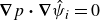 $\boldsymbol{\nabla }p\boldsymbol{\cdot }\boldsymbol{\nabla }\hat {\psi }_i=0$
,
$\boldsymbol{\nabla }p\boldsymbol{\cdot }\boldsymbol{\nabla }\hat {\psi }_i=0$
, $i=1,2$
), and so provides a structured, orthogonal 3-D Lagrangian coordinate system
$i=1,2$
), and so provides a structured, orthogonal 3-D Lagrangian coordinate system $\boldsymbol \zeta \equiv (\zeta _1,\zeta _2,\zeta _3)\equiv (\hat \psi _1,\hat \psi _2,p)$
. The transform from Eulerian space
$\boldsymbol \zeta \equiv (\zeta _1,\zeta _2,\zeta _3)\equiv (\hat \psi _1,\hat \psi _2,p)$
. The transform from Eulerian space $\boldsymbol{x}=(x_1,x_2,x_3)$
to
$\boldsymbol{x}=(x_1,x_2,x_3)$
to $\boldsymbol \zeta$
completely quantifies advective mixing. We note that the coordinate system
$\boldsymbol \zeta$
completely quantifies advective mixing. We note that the coordinate system $\boldsymbol \zeta$
naturally resolves advective mixing in rough fractures and intersections of variable aperture fractures, as the 2-D boundaries of 3-D fractures correspond to coherent
$\boldsymbol \zeta$
naturally resolves advective mixing in rough fractures and intersections of variable aperture fractures, as the 2-D boundaries of 3-D fractures correspond to coherent $\hat \psi _1$
- or
$\hat \psi _1$
- or $\hat \psi _2$
-streamsurfaces. Streamline coordinates will be used extensively to quantify advective mixing in 3-D DFNs.
$\hat \psi _2$
-streamsurfaces. Streamline coordinates will be used extensively to quantify advective mixing in 3-D DFNs.
2.4. Intersection and fracture mixing
We consider simple 3-D DFNs (figure 2) as a basis to develop methods that extend to arbitrarily large networks. Despite their simplicity, these systems exhibit two distinct mixing mechanisms controlled by fracture geometry and connectivity. In the top configuration, streamline routing within fractures produces large-scale mixing at the fracture length scale $L$
, whereas in the bottom configuration, routing at intersections induces fine-scale mixing at the aperture scale
$L$
, whereas in the bottom configuration, routing at intersections induces fine-scale mixing at the aperture scale $\ell$
. These define fracture mixing (at length scale
$\ell$
. These define fracture mixing (at length scale $L$
) and intersection mixing (at length scale
$L$
) and intersection mixing (at length scale $\ell$
).
$\ell$
).
We denote the 2-D cross-section immediately adjacent to an intersection as a face $f_n$
(
$f_n$
( $n=1{:}N_f$
). Under the assumption of negligible longitudinal pressure gradients along intersections, the velocity field
$n=1{:}N_f$
). Under the assumption of negligible longitudinal pressure gradients along intersections, the velocity field $\boldsymbol{v}(\boldsymbol{x})$
is orthogonal to all faces
$\boldsymbol{v}(\boldsymbol{x})$
is orthogonal to all faces $f_n$
. Hence, each face is classified as an inlet
$f_n$
. Hence, each face is classified as an inlet $f_n^i$
or outlet
$f_n^i$
or outlet $f_n^o$
relative to its adjacent intersection; by convention, we define an inflow face (i.e. that with fluid flowing into the network) to be an outlet face
$f_n^o$
relative to its adjacent intersection; by convention, we define an inflow face (i.e. that with fluid flowing into the network) to be an outlet face $f_n^o$
and likewise an outflow face (i.e. that with fluid flowing out of the network) to be an inlet face
$f_n^o$
and likewise an outflow face (i.e. that with fluid flowing out of the network) to be an inlet face $f_n^i$
. Streamlines thus traverse the network periodically encountering outlet faces, fractures, inlet faces and intersections in sequence.
$f_n^i$
. Streamlines thus traverse the network periodically encountering outlet faces, fractures, inlet faces and intersections in sequence.
(a) Schematic of two intersecting fractures $F_1$
,
$F_1$
, $F_2$
of characteristic aperture
$F_2$
of characteristic aperture $\ell$
and width
$\ell$
and width $L$
forming an intersection
$L$
forming an intersection $I_1$
. Streamlines are separated by a continuous line of hyperbolic stagnation points
$I_1$
. Streamlines are separated by a continuous line of hyperbolic stagnation points $\boldsymbol{x}_p$
at the fracture intersection, and the associated stable (blue) and unstable (red) hyperbolic manifolds route surrounding streamlines (black) to their respective outlet faces. (b) Schematic detailing intersection
$\boldsymbol{x}_p$
at the fracture intersection, and the associated stable (blue) and unstable (red) hyperbolic manifolds route surrounding streamlines (black) to their respective outlet faces. (b) Schematic detailing intersection $I_1$
shown in panel (a) depicting the inlet faces
$I_1$
shown in panel (a) depicting the inlet faces $f^i_1$
,
$f^i_1$
, $f^i_2$
associated with fracture
$f^i_2$
associated with fracture $F_1$
and outlet faces
$F_1$
and outlet faces $f^o_1$
,
$f^o_1$
, $f^o_2$
associated with fracture
$f^o_2$
associated with fracture $F_2$
. Also shown are the local streamfunctions
$F_2$
. Also shown are the local streamfunctions $\psi _{1,n}\in [0,1]$
,
$\psi _{1,n}\in [0,1]$
, $\psi _{2,n}\in [0,1]$
, and associated
$\psi _{2,n}\in [0,1]$
, and associated $\psi _{1,n}$
- and
$\psi _{1,n}$
- and $\psi _{2,n}$
-streamsurfaces that are respectively oriented along the fracture width
$\psi _{2,n}$
-streamsurfaces that are respectively oriented along the fracture width $L$
and fracture aperture
$L$
and fracture aperture $\ell$
of each face. Similar to panel (a), the hyperbolic point
$\ell$
of each face. Similar to panel (a), the hyperbolic point $\boldsymbol{x}_p$
and associated manifolds route streamlines into downstream outlet faces. Local streamfunctions
$\boldsymbol{x}_p$
and associated manifolds route streamlines into downstream outlet faces. Local streamfunctions $\psi _2$
govern routing of streamlines, which leads to cutting and shuffling of fluid elements leaving
$\psi _2$
govern routing of streamlines, which leads to cutting and shuffling of fluid elements leaving $f^i_1$
,
$f^i_1$
, $f^i_2$
and arriving at
$f^i_2$
and arriving at $f^o_1$
,
$f^o_1$
, $f^o_2$
.
$f^o_2$
.

Schematic of the complete set of distinct streamline topologies in a cross-section (a–d) X-, (e–f) T- and (g) L-shaped intersection. Each cross-section corresponds to a $\hat \psi _1$
-streamsurface, hence, the streamline topology is the same as that for a steady 2-D flow. Stagnation points
$\hat \psi _1$
-streamsurface, hence, the streamline topology is the same as that for a steady 2-D flow. Stagnation points $\boldsymbol{x}_p$
and corresponding (blue) stable and (red) unstable hyperbolic manifolds (which act as separating streamlines) act to route fluid parcels through inlet
$\boldsymbol{x}_p$
and corresponding (blue) stable and (red) unstable hyperbolic manifolds (which act as separating streamlines) act to route fluid parcels through inlet $f_n^i$
and outlet
$f_n^i$
and outlet $f_n^o$
faces of the intersection. Black arrows indicate flow direction.
$f_n^o$
faces of the intersection. Black arrows indicate flow direction.

As shown in figure 3, intersection mixing is governed by streamline routing between inlet and outlet faces. Owing to the epi-2-D nature of isotropic Darcy flow, streamlines lie on $\hat \psi _1$
-streamsurfaces and exhibit the topology of steady 2-D planar flow. Within each surface, routing is determined by separatrices connected to the stagnation point
$\hat \psi _1$
-streamsurfaces and exhibit the topology of steady 2-D planar flow. Within each surface, routing is determined by separatrices connected to the stagnation point $\boldsymbol{x}_p$
. This topology is invariant across
$\boldsymbol{x}_p$
. This topology is invariant across $\hat \psi _1$
-streamsurfaces, such that zero-dimensional (0-D) stagnation points and 1-D separatrices correspond to 1-D stagnation lines and 2-D separating
$\hat \psi _1$
-streamsurfaces, such that zero-dimensional (0-D) stagnation points and 1-D separatrices correspond to 1-D stagnation lines and 2-D separating $\hat \psi _1$
-streamsurfaces spanning the 3-D intersection. Intersections of two fractures may also form X-, T- or L-shaped cross-sections, with four, three or two faces, respectively (figure 4). These admit seven distinct planar streamline topologies, distinguished by inlet–outlet configuration and stagnation structure. As only
$\hat \psi _1$
-streamsurfaces spanning the 3-D intersection. Intersections of two fractures may also form X-, T- or L-shaped cross-sections, with four, three or two faces, respectively (figure 4). These admit seven distinct planar streamline topologies, distinguished by inlet–outlet configuration and stagnation structure. As only $\hat \psi _2$
varies within each
$\hat \psi _2$
varies within each $\hat \psi _1$
-streamsurface, it fully characterises streamline routing during intersection mixing.
$\hat \psi _1$
-streamsurface, it fully characterises streamline routing during intersection mixing.
Similar to intersection mixing, fracture mixing is driven by the routing of streamlines within fractures to different faces $f_n$
. As streamlines are confined to
$f_n$
. As streamlines are confined to $\hat \psi _2$
-streamsurfaces (figure 5
a), streamline topology within each fracture is the same as that of a 2-D planar flow. Within each
$\hat \psi _2$
-streamsurfaces (figure 5
a), streamline topology within each fracture is the same as that of a 2-D planar flow. Within each $\hat \psi _2$
-streamsurface, streamlines are routed by separating streamlines connected to stagnation points and other critical points (defined in §§ 2.5). Similar to intersection mixing, these 0-D critical points and 1-D separating streamlines manifest as 1-D critical lines and 2-D separating
$\hat \psi _2$
-streamsurface, streamlines are routed by separating streamlines connected to stagnation points and other critical points (defined in §§ 2.5). Similar to intersection mixing, these 0-D critical points and 1-D separating streamlines manifest as 1-D critical lines and 2-D separating $\hat \psi _1$
-streamsurfaces across the full 3-D fracture.
$\hat \psi _1$
-streamsurfaces across the full 3-D fracture.
As shown in figure 5(a), even simple fractures (e.g. $F_2$
) connecting a single source (
$F_2$
) connecting a single source ( $I_1$
) and sink (
$I_1$
) and sink ( $I_2$
) contain multiple separatrices that partition flow between faces, yielding more complex topologies than for intersection mixing (figure 4). Figure 5(b) illustrates the treatment of dead-end fractures under the assumption of constant pressure along intersections. By splitting the intersection
$I_2$
) contain multiple separatrices that partition flow between faces, yielding more complex topologies than for intersection mixing (figure 4). Figure 5(b) illustrates the treatment of dead-end fractures under the assumption of constant pressure along intersections. By splitting the intersection $I_1$
in figure 5(a) into ‘inflow’ and ‘outflow’ components (with respect to the dead-end fracture
$I_1$
in figure 5(a) into ‘inflow’ and ‘outflow’ components (with respect to the dead-end fracture $F_1$
), streamlines are routed from
$F_1$
), streamlines are routed from $I_1$
to
$I_1$
to $I_3$
via the same mechanism as in non-dead-end fractures. Figure 6(a) shows typical streamlines (computed using DFN.lab) for an X-shaped intersection. The flux-weighted random streamline routing in DFN.lab distributes red and blue streamlines across both outlets, whereas deterministic routing (figure 4
b) directs all streamlines of a given type into at least one outlet. This discrepancy highlights the limitations of random routing for representing advective – and thus also finite-
$I_3$
via the same mechanism as in non-dead-end fractures. Figure 6(a) shows typical streamlines (computed using DFN.lab) for an X-shaped intersection. The flux-weighted random streamline routing in DFN.lab distributes red and blue streamlines across both outlets, whereas deterministic routing (figure 4
b) directs all streamlines of a given type into at least one outlet. This discrepancy highlights the limitations of random routing for representing advective – and thus also finite- $Pe$
– mixing. Figure 6(b) shows the corresponding routing in a dead-end fracture, where
$Pe$
– mixing. Figure 6(b) shows the corresponding routing in a dead-end fracture, where $I_3$
is split into
$I_3$
is split into $I_3$
and
$I_3$
and $I_4$
; the resulting intersection graphs are shown in figure 6(c), with intersections as nodes and fractures as edges.
$I_4$
; the resulting intersection graphs are shown in figure 6(c), with intersections as nodes and fractures as edges.
(a) Schematic of a simple fracture network (at the fracture scale $L$
) comprising fractures
$L$
) comprising fractures $F_n$
(where
$F_n$
(where $F_1$
and
$F_1$
and $F_3$
respectively are inlet and outlet fractures) and intersections
$F_3$
respectively are inlet and outlet fractures) and intersections $I_m$
(green lines), separating streamlines (black lines) and critical points (black dots). Separating streamlines route fluid ‘parcels’ from ‘source’ intersection faces to different ‘sink’ intersection faces. Stagnation (critical) points are denoted
$I_m$
(green lines), separating streamlines (black lines) and critical points (black dots). Separating streamlines route fluid ‘parcels’ from ‘source’ intersection faces to different ‘sink’ intersection faces. Stagnation (critical) points are denoted $\boldsymbol{x}_p$
(with corresponding hyperbolic stable (blue) and unstable (red) manifolds), while terminal and interior critical points are unlabelled. All separating streamlines either originate or terminate at stagnation or terminal critical points. (b) Same schematic as panel (a), but with a dead-end fracture (
$\boldsymbol{x}_p$
(with corresponding hyperbolic stable (blue) and unstable (red) manifolds), while terminal and interior critical points are unlabelled. All separating streamlines either originate or terminate at stagnation or terminal critical points. (b) Same schematic as panel (a), but with a dead-end fracture ( $F_1$
) which is treated by splitting intersection
$F_1$
) which is treated by splitting intersection $I_1$
in panel (a) into an ‘outflow’ intersection
$I_1$
in panel (a) into an ‘outflow’ intersection $I_1$
and an ‘inflow’ intersection
$I_1$
and an ‘inflow’ intersection $I_3$
, with streamlines routed in
$I_3$
, with streamlines routed in $F_1$
from
$F_1$
from $I_1$
to
$I_1$
to $I_3$
.
$I_3$
.

(a) Random, flux-weighted routing of streamlines through an X-shaped intersection, computed using DFN.lab. Note that random routing directs both red and blue inlet streamlines into both outlet fractures, which cannot occur for deterministic streamlines. (b) Random, flux-weighted routing of streamlines through a dead-end fracture $F_3$
, computed using DFN.lab. Note that intersection
$F_3$
, computed using DFN.lab. Note that intersection $I_3$
in panel (a) can be split into two separate fractures
$I_3$
in panel (a) can be split into two separate fractures $I_3$
,
$I_3$
, $I_4$
. (c) Intersection graphs
$I_4$
. (c) Intersection graphs ${\mathcal{G}_I}$
depicting (top) the X-shaped intersection shown in panel (a) and (bottom) the X-shaped intersection with dead-end shown in panel (b).
${\mathcal{G}_I}$
depicting (top) the X-shaped intersection shown in panel (a) and (bottom) the X-shaped intersection with dead-end shown in panel (b).

Despite the differences in complexity of streamline topology and the presence of dead-end fractures, fracture mixing is very similar to intersection mixing in that it is driven by streamline routing. Hence, critical points, lines and surfaces control both intersection and fracture mixing in 3-D DFNs.
2.5. Critical points, lines and surfaces
The inherent topological complexity of fracture networks gives rise to critical features – stagnation points and lines, separating streamlines and streamsurfaces (figures 3, 4, 5) – that control streamline routing and advective mixing. In 3-D DFNs, stagnation points $\boldsymbol{x}_p$
arise at junctions within fractures, which are connected to separating streamlines that route fluid parcels to/from different intersections within the fracture. In addition to stagnation points, terminal critical points shown (figure 5
a) arise at the termini of 1-D intersections and differentiate flows into or out of different faces
$\boldsymbol{x}_p$
arise at junctions within fractures, which are connected to separating streamlines that route fluid parcels to/from different intersections within the fracture. In addition to stagnation points, terminal critical points shown (figure 5
a) arise at the termini of 1-D intersections and differentiate flows into or out of different faces $f_n$
on each side of an intersection. Hence, in fracture flows, there are additional separating streamlines that originate or terminate at terminal critical points, and these separating streamlines can either originate or terminate at stagnation points, terminal points or midway along faces
$f_n$
on each side of an intersection. Hence, in fracture flows, there are additional separating streamlines that originate or terminate at terminal critical points, and these separating streamlines can either originate or terminate at stagnation points, terminal points or midway along faces $f_n$
, forming the interior critical points shown in figure 5(a). Together, these critical points and their associated separating streamlines act to route fluid elements from parts of outlet faces
$f_n$
, forming the interior critical points shown in figure 5(a). Together, these critical points and their associated separating streamlines act to route fluid elements from parts of outlet faces $f_n^o$
to parts of inlet faces
$f_n^o$
to parts of inlet faces $f_n^i$
, leading to discontinuous mixing as discussed in the following.
$f_n^i$
, leading to discontinuous mixing as discussed in the following.
2.6. Discontinuous mixing in fractured media
Although stretching and folding (SF) of fluid elements around stagnation points in 3-D DFNs cannot generate significant chaotic advection, it does generate discontinuous mixing (Sturman Reference Sturman2012; Smith et al. Reference Smith, Umbanhowar, Lueptow and Ottino2019), involving cutting-and-shuffling (CS) of fluid elements. CS is akin to shuffling of a deck of infinitely divisible cards, where an initially continuous set of streamlines is ‘cut’ into a set of streamline ‘parcels’ that are then ‘shuffled’ and recombined in a different arrangement. In the language of ergodic theory (Arnold & Avez Reference Arnold and Avez1968), mixing via CS is weak mixing, as compared with strong mixing under SF; however, CS mixing can still lead to rapid and complete (ergodic) advective mixing (Sturman Reference Sturman2012; Smith et al. Reference Smith, Umbanhowar, Lueptow and Ottino2019).
(a) Stretching and folding (SF) due to hold-up of a fluid element (shaded, shown at successive times) at the stagnation point $\boldsymbol{x}_p$
of a fracture intersection. As the ‘legs’ of the fluid element are advected downstream into separate outlets, the element is stretched exponentially in time at
$\boldsymbol{x}_p$
of a fracture intersection. As the ‘legs’ of the fluid element are advected downstream into separate outlets, the element is stretched exponentially in time at $\boldsymbol{x}_p$
. Further downstream, the legs of the element are effectively disconnected (‘cut’) when their intersection with an arbitrary planar cross-section (vertical dashed line)
$\boldsymbol{x}_p$
. Further downstream, the legs of the element are effectively disconnected (‘cut’) when their intersection with an arbitrary planar cross-section (vertical dashed line) $P_o$
is considered. (b) Merger of two fluid elements (dark and light shading) as they approach a stagnation point
$P_o$
is considered. (b) Merger of two fluid elements (dark and light shading) as they approach a stagnation point $\boldsymbol{x}_p$
of a fracture intersection. Within the planar cross-section
$\boldsymbol{x}_p$
of a fracture intersection. Within the planar cross-section $P_o$
, these elements are essentially merged next to each other (as the width of the separating fluid decays exponentially at
$P_o$
, these elements are essentially merged next to each other (as the width of the separating fluid decays exponentially at $\boldsymbol{x}_p$
) effectively ‘shuffling’ fluid elements together. In unison, the stretching and folding (SF) motions shown in panels (a) and (b) manifest as cutting and shuffling (CS) actions when considered within the cross-section
$\boldsymbol{x}_p$
) effectively ‘shuffling’ fluid elements together. In unison, the stretching and folding (SF) motions shown in panels (a) and (b) manifest as cutting and shuffling (CS) actions when considered within the cross-section $P_o$
.
$P_o$
.

Figure 7(a) illustrates how stretching and folding (SF) near a stagnation point $\boldsymbol{x}_p$
manifests as cutting and shuffling (CS): part of a fluid element is held up at
$\boldsymbol{x}_p$
manifests as cutting and shuffling (CS): part of a fluid element is held up at $\boldsymbol{x}_p$
, stretched and folded across the intersection, and then ‘cut’ downstream as its legs disconnect in the cross-section
$\boldsymbol{x}_p$
, stretched and folded across the intersection, and then ‘cut’ downstream as its legs disconnect in the cross-section $P_0$
. Conversely, two fluid elements passing near
$P_0$
. Conversely, two fluid elements passing near $\boldsymbol{x}_p$
(figure 7
b) are effectively merged, ‘shuffling’ them together. Thus, the local SF dynamics project as CS in
$\boldsymbol{x}_p$
(figure 7
b) are effectively merged, ‘shuffling’ them together. Thus, the local SF dynamics project as CS in $P_0$
. The fine-scale interleaving in figure 2(c) exemplifies CS at intersections, while hold-up at fracture critical points produces large-scale CS (figure 2
a). A similar mechanism occurs in open porous networks, though these admit both SF and CS (Lester et al. Reference Lester, Heyman, Méheust and Le Borgne2025a
).
$P_0$
. The fine-scale interleaving in figure 2(c) exemplifies CS at intersections, while hold-up at fracture critical points produces large-scale CS (figure 2
a). A similar mechanism occurs in open porous networks, though these admit both SF and CS (Lester et al. Reference Lester, Heyman, Méheust and Le Borgne2025a
).
Although persistent exponential stretching is absent in 3-D DFNs, fluctuating stretching arises from local velocity variations. CS without deformation corresponds to piecewise isometries (PWIs), while CS with stretching yields piecewise smooth (PWS) transforms (Kreczak, Sturman & Wilson Reference Kreczak, Sturman and Wilson2017). In DFNs, this stretching is sub-exponential and bounded, reflecting non-chaotic flow. Sections 3 and 4 show that mixing is exactly described by PWS transforms which are quantified via a graph-based representation of advective mixing that is developed in the following section.
(a) Intersection of local streamfunctions ( $\psi _{1,n},\psi _{2,n}$
) within the face
$\psi _{1,n},\psi _{2,n}$
) within the face $f_n$
of the fracture network (with dimensions
$f_n$
of the fracture network (with dimensions ${\sim} L\,\times {\sim} \ell$
) that define a streamline with local velocity
${\sim} L\,\times {\sim} \ell$
) that define a streamline with local velocity $\boldsymbol{v}_n$
. (b) Distribution of the local
$\boldsymbol{v}_n$
. (b) Distribution of the local $\psi _{1,n}$
(vertical lines) and
$\psi _{1,n}$
(vertical lines) and $\psi _{2,n}$
(horizontal lines) streamsurfaces over the face
$\psi _{2,n}$
(horizontal lines) streamsurfaces over the face $f_n$
of a rough fracture of variable aperture. The mapping from local spatial coordinates
$f_n$
of a rough fracture of variable aperture. The mapping from local spatial coordinates $(x\prime_{1,n},x\prime_{2,n})$
in panel (b) to local streamfunction coordinates
$(x\prime_{1,n},x\prime_{2,n})$
in panel (b) to local streamfunction coordinates $(\psi _{1,n},\psi _{2,n})$
in panel (c) generates a structured orthogonal coordinate system over face
$(\psi _{1,n},\psi _{2,n})$
in panel (c) generates a structured orthogonal coordinate system over face $f_n$
. Note this structured grid is also depicted throughout the intersection shown in figure 3(b).
$f_n$
. Note this structured grid is also depicted throughout the intersection shown in figure 3(b).

3. Graph representation of advective mixing
To develop a graph representation of mixing, we begin by labelling the $N_F$
fractures within the fracture network as
$N_F$
fractures within the fracture network as $F_n$
with
$F_n$
with $n=1:N_F$
and the
$n=1:N_F$
and the $N_I$
intersections as
$N_I$
intersections as $I_n$
with
$I_n$
with $n=1:N_I$
(where
$n=1:N_I$
(where $N_F\leqslant N_I$
), where, as shown in figure 1(b), inlets and outlets to the network are also considered as intersections. The number of inlet, interior and outlet intersections are respectively denoted
$N_F\leqslant N_I$
), where, as shown in figure 1(b), inlets and outlets to the network are also considered as intersections. The number of inlet, interior and outlet intersections are respectively denoted $N_{I_i},N_{I_b},N_{I_o}$
, such that
$N_{I_i},N_{I_b},N_{I_o}$
, such that $N_I=N_{I_i}+N_{I_b}+N_{I_o}$
, and the
$N_I=N_{I_i}+N_{I_b}+N_{I_o}$
, and the $N_I$
intersections
$N_I$
intersections $I_n$
are ordered such that
$I_n$
are ordered such that $n=1:N_{I_i}$
are the inlet intersections,
$n=1:N_{I_i}$
are the inlet intersections, $n=N_{I_i}+1:N_{I_i}+N_{I_b}$
are the interior intersections, and
$n=N_{I_i}+1:N_{I_i}+N_{I_b}$
are the interior intersections, and $n=N_{I}-N_{I_o}:N_I$
are the outlet intersections.
$n=N_{I}-N_{I_o}:N_I$
are the outlet intersections.
3.1. Global and local streamfunctions
Under this framework, the invariant streamfunctions $(\hat \psi _1$
,
$(\hat \psi _1$
, $\hat \psi _2)\in [0,1]\times [0,1]$
in (2.3) are termed global streamfunctions as they uniquely label each streamline over the entire fracture network. In addition to these global streamfunctions, we also define local streamfunctions
$\hat \psi _2)\in [0,1]\times [0,1]$
in (2.3) are termed global streamfunctions as they uniquely label each streamline over the entire fracture network. In addition to these global streamfunctions, we also define local streamfunctions $(\psi _{1,n},\psi _{2,n})$
(shown in figure 8) over each face
$(\psi _{1,n},\psi _{2,n})$
(shown in figure 8) over each face $f_n$
of the network (e.g. figures 2
b and 2
d). These local streamfunctions characterise the local distribution of streamlines over
$f_n$
of the network (e.g. figures 2
b and 2
d). These local streamfunctions characterise the local distribution of streamlines over $f_n$
and so facilitate quantification of advective mixing.
$f_n$
and so facilitate quantification of advective mixing.
The local streamfunctions are also normal $(\psi _{1,n},\psi _{2,n})\in [0,1]\times [0,1]$
) and orthogonal (
$(\psi _{1,n},\psi _{2,n})\in [0,1]\times [0,1]$
) and orthogonal ( $\boldsymbol{\nabla }\psi _{1,n}\boldsymbol{\cdot }\boldsymbol{\nabla }\psi _{2,n}=0$
), and are quantified in terms of the local velocity field
$\boldsymbol{\nabla }\psi _{1,n}\boldsymbol{\cdot }\boldsymbol{\nabla }\psi _{2,n}=0$
), and are quantified in terms of the local velocity field $\boldsymbol{v}_n$
as
$\boldsymbol{v}_n$
as
 \begin{equation} \boldsymbol{v}_n(\boldsymbol{x})\equiv \boldsymbol{v}(\boldsymbol{x})\,\,\forall \,\,\boldsymbol{x}\in S_n, \end{equation}
where $S_n$
is the 2-D surface that spans the face
$S_n$
is the 2-D surface that spans the face $f_n$
. Consistent with the dual streamfunction representation (2.3), the local streamfunctions
$f_n$
. Consistent with the dual streamfunction representation (2.3), the local streamfunctions $(\psi _{1,n},\psi _{2,n})$
are then defined as
$(\psi _{1,n},\psi _{2,n})$
are then defined as
 \begin{equation} \boldsymbol{v}_n(\boldsymbol{x})\equiv Q_n\boldsymbol{\nabla }\psi _{1,n}(\boldsymbol{x})\times \boldsymbol{\nabla }\psi _{2,n}(\boldsymbol{x}),\quad n=1:N_{I},\quad \psi _{i,n}\in [0,1],\quad i=1,2, \end{equation}
where $Q_n$
is the volumetric flow rate through face
$Q_n$
is the volumetric flow rate through face $f_n$
. From (3.2), the face
$f_n$
. From (3.2), the face $f_n$
is bound by four stream surfaces:
$f_n$
is bound by four stream surfaces: $\psi _{1,n}=0$
,
$\psi _{1,n}=0$
, $\psi _{1,n}=1$
,
$\psi _{1,n}=1$
, $\psi _{2,n}=0$
,
$\psi _{2,n}=0$
, $\psi _{2,n}=1$
. As
$\psi _{2,n}=1$
. As $\boldsymbol{\nabla }\psi _{1,n}$
and
$\boldsymbol{\nabla }\psi _{1,n}$
and $\boldsymbol{\nabla }\psi _{2,n}$
are both parallel to
$\boldsymbol{\nabla }\psi _{2,n}$
are both parallel to $S_n$
, the fluid flow rate
$S_n$
, the fluid flow rate $Q_n$
through this face is then conserved (Bear Reference Bear1972)
$Q_n$
through this face is then conserved (Bear Reference Bear1972)
 \begin{equation} Q_n=\iint _{S_n}\boldsymbol{v}_n(\boldsymbol{x})\boldsymbol{\cdot }\text{d}\boldsymbol{S}=Q_n\int _0^1\int _0^1\text{d}\psi _{1,n}\,\text{d}\psi _{2,n}=Q_n. \end{equation}
The local streamfunctions $(\psi _{1,n},\psi _{2,n})$
represent a local re-labelling of the global streamfunctions over face
$(\psi _{1,n},\psi _{2,n})$
represent a local re-labelling of the global streamfunctions over face $f_n$
. For example, if the
$f_n$
. For example, if the $\hat \psi _1$
-streamsurface
$\hat \psi _1$
-streamsurface $\hat \psi _1=a=$
const. intersects face
$\hat \psi _1=a=$
const. intersects face $f_n$
, this streamsurface also satisfies
$f_n$
, this streamsurface also satisfies $\psi _{1,n}=b=$
const., but in general
$\psi _{1,n}=b=$
const., but in general $a\neq b$
. Hence, a streamline may be labelled by the unique pair of global streamfunctions
$a\neq b$
. Hence, a streamline may be labelled by the unique pair of global streamfunctions $(\hat \psi _{1},\hat \psi _{2})$
that are invariant over the entire network, but this streamline also traverses the fracture network via a sequence of faces
$(\hat \psi _{1},\hat \psi _{2})$
that are invariant over the entire network, but this streamline also traverses the fracture network via a sequence of faces $f_{n_1}, f_{n_2},\ldots$
with local streamfunction values
$f_{n_1}, f_{n_2},\ldots$
with local streamfunction values $(\psi _{1,n_1},\psi _{2,n_1}),(\psi _{1,n_2},\psi _{2,n_2}),\ldots$
. As such, the global streamfunctions
$(\psi _{1,n_1},\psi _{2,n_1}),(\psi _{1,n_2},\psi _{2,n_2}),\ldots$
. As such, the global streamfunctions $(\hat \psi _1,\hat \psi _2)$
are used to label a given streamline, while the local streamfunctions
$(\hat \psi _1,\hat \psi _2)$
are used to label a given streamline, while the local streamfunctions $(\psi _{1,n},\psi _{2,n})$
are used to characterise the local position of that streamline in face
$(\psi _{1,n},\psi _{2,n})$
are used to characterise the local position of that streamline in face $f_n$
. Hence, advective mixing can be quantified by the evolution of
$f_n$
. Hence, advective mixing can be quantified by the evolution of $(f_n,\psi _{1,n},\psi _{2,n})$
for a given streamline.
$(f_n,\psi _{1,n},\psi _{2,n})$
for a given streamline.
As illustrated in figure 8, $\psi _{1,n}$
varies along the fracture width (
$\psi _{1,n}$
varies along the fracture width ( ${\sim} L$
) of face
${\sim} L$
) of face $f_n$
and
$f_n$
and $\psi _{2,n}$
varies along the fracture aperture (
$\psi _{2,n}$
varies along the fracture aperture ( ${\sim} \ell$
), with streamlines arising at the intersection of local
${\sim} \ell$
), with streamlines arising at the intersection of local $\psi _{1,n}$
- and
$\psi _{1,n}$
- and $\psi _{2,n}$
-streamsurfaces. We also introduce the local Eulerian spatial coordinates
$\psi _{2,n}$
-streamsurfaces. We also introduce the local Eulerian spatial coordinates $(x^\prime_{1,n},x^\prime_{2,n})\in [0,{\sim} L]\times [0,{\sim} \ell ]$
(figure 8
b) that span
$(x^\prime_{1,n},x^\prime_{2,n})\in [0,{\sim} L]\times [0,{\sim} \ell ]$
(figure 8
b) that span $f_n$
and their dimensionless counterparts
$f_n$
and their dimensionless counterparts $(x_{1,n},x_{2,n})\in [0,1]\times [0,1]$
. Figure 8(c) shows that the mapping from local spatial coordinates
$(x_{1,n},x_{2,n})\in [0,1]\times [0,1]$
. Figure 8(c) shows that the mapping from local spatial coordinates $(x^\prime_{1,n},x^\prime_{2,n})$
to local streamfunction coordinates
$(x^\prime_{1,n},x^\prime_{2,n})$
to local streamfunction coordinates $(\psi _{1,n},\psi _{2,n})$
allows rough fractures with variable aperture to be mapped onto a structured orthogonal grid. As shown in figure 3(b), this means that even if rough, 3-D intersections are spanned and bounded by a structured orthogonal grid of
$(\psi _{1,n},\psi _{2,n})$
allows rough fractures with variable aperture to be mapped onto a structured orthogonal grid. As shown in figure 3(b), this means that even if rough, 3-D intersections are spanned and bounded by a structured orthogonal grid of $\hat \psi _1$
- and
$\hat \psi _1$
- and $\hat \psi _2$
-streamsurfaces, where the
$\hat \psi _2$
-streamsurfaces, where the $\hat \psi _1$
-streamsurfaces are coherent 2-D cross-sections of the intersection.
$\hat \psi _1$
-streamsurfaces are coherent 2-D cross-sections of the intersection.
For fracture networks with only one inlet fracture (i.e. $N_{I_i}=1$
), the outlet face (where fluid enters the network) is defined as
$N_{I_i}=1$
), the outlet face (where fluid enters the network) is defined as $f_n=f^o_1$
with flow rate
$f_n=f^o_1$
with flow rate $Q_1^o$
. Hence, the total network flow rate is
$Q_1^o$
. Hence, the total network flow rate is $Q=Q^o_1$
, and from (2.3), (3.2), we can also define the global and local streamfunctions to coincide over face
$Q=Q^o_1$
, and from (2.3), (3.2), we can also define the global and local streamfunctions to coincide over face $f_n$
as
$f_n$
as
 \begin{align} \psi _{1,n=1}\equiv \hat \psi _1 && \psi _{2,n=1}\equiv \hat \psi _2. \end{align}
Conversely, for fracture networks with multiple inlet fractures ( $N_{I_i}\gt 1$
), the corresponding outlet faces can be defined as
$N_{I_i}\gt 1$
), the corresponding outlet faces can be defined as $f_n=f^o_n$
with
$f_n=f^o_n$
with $n=1:I_i$
, and the total network flow rate
$n=1:I_i$
, and the total network flow rate $Q$
is
$Q$
is
 \begin{equation} Q=\sum _{n=1}^{N_{I_i}}Q^o_{n}, \end{equation}
where $Q_{n,1}^o$
is the total flowrate through face
$Q_{n,1}^o$
is the total flowrate through face $f_n^o$
. From (2.3), (3.2), we can uniquely define the global streamfunctions by spanning the
$f_n^o$
. From (2.3), (3.2), we can uniquely define the global streamfunctions by spanning the $\hat \psi _1$
streamfunction over the
$\hat \psi _1$
streamfunction over the $N_{I_i}$
ordered inlets as
$N_{I_i}$
ordered inlets as
 \begin{align} \psi _{1,m}\equiv \frac {1}{Q^o_{m,1}}\left (Q\,\hat \psi _1-\sum _{n=1}^{m-1}Q^o_{n,1}\right ) && \psi _{2,m}\equiv \hat \psi _2,\quad m\in [1:N_{I_i}], \end{align}
where $m$
is the index of the outlet face
$m$
is the index of the outlet face $f^o_m$
corresponding to
$f^o_m$
corresponding to $\psi _{1,m}$
,
$\psi _{1,m}$
, $\hat \psi _1$
. Note the flow rates in (3.6) arise from normalisation of the streamfunctions in (2.3), (3.2). The local streamfunctions
$\hat \psi _1$
. Note the flow rates in (3.6) arise from normalisation of the streamfunctions in (2.3), (3.2). The local streamfunctions $(\psi _{1,n},\psi _{2,n})$
for the remaining faces (i.e.
$(\psi _{1,n},\psi _{2,n})$
for the remaining faces (i.e. $n\gt N_{I_i}$
) in the network are defined by (3.2). Together, the local and global streamfunctions can be used to quantify intersection and fracture mixing.
$n\gt N_{I_i}$
) in the network are defined by (3.2). Together, the local and global streamfunctions can be used to quantify intersection and fracture mixing.
3.2. Intersection and fracture mixing maps
We first develop a method to route streamlines between faces in the network. As a streamline is advected from face $f_j$
(with local streamfunctions
$f_j$
(with local streamfunctions $\psi _{1,j},\psi _{2,j}$
) in the network, the next face
$\psi _{1,j},\psi _{2,j}$
) in the network, the next face $f_k$
it encounters (and local streamfunctions
$f_k$
it encounters (and local streamfunctions $\psi _{1,k},\psi _{2,k}$
) is determined by streamline routing. The relationship between these faces and local streamfunctions can be efficiently encoded via two classes of algebraic maps we term mixing maps. If face
$\psi _{1,k},\psi _{2,k}$
) is determined by streamline routing. The relationship between these faces and local streamfunctions can be efficiently encoded via two classes of algebraic maps we term mixing maps. If face $f_j$
is an inlet face, the streamline then passes through an intersection and
$f_j$
is an inlet face, the streamline then passes through an intersection and $(f_k,\psi _{1,k},\psi _{2,k})$
is determined by an intersection mixing map
$(f_k,\psi _{1,k},\psi _{2,k})$
is determined by an intersection mixing map ${\mathcal{M}_I}$
. Conversely, if face
${\mathcal{M}_I}$
. Conversely, if face $f_j$
is an outlet face, the streamline then passes through a fracture and
$f_j$
is an outlet face, the streamline then passes through a fracture and $(f_k,\psi _{1,k},\psi _{2,k})$
is determined by a fracture mixing map
$(f_k,\psi _{1,k},\psi _{2,k})$
is determined by a fracture mixing map ${\mathcal{M}_F}$
. As streamlines are routed through either intersections or fractures with fixed global streamfunctions
${\mathcal{M}_F}$
. As streamlines are routed through either intersections or fractures with fixed global streamfunctions $(\hat \psi _1,\hat \psi _2)$
, the relationship between the local streamfunctions at faces
$(\hat \psi _1,\hat \psi _2)$
, the relationship between the local streamfunctions at faces $f_j$
and
$f_j$
and $f_k$
is given by the mappings between the global and local streamfunctions at these faces.
$f_k$
is given by the mappings between the global and local streamfunctions at these faces.
For the case of intersection mixing, we show in Appendix B that if the spatial distribution of areal fluxes,
 \begin{equation} q_n(x_1)\equiv \int _0^1 ||\boldsymbol{v}_n|| \,\text{d}\psi _{2,n}=Q_n\boldsymbol{\nabla }\psi _{1,n}, \end{equation}
between the inlet face $f_j$
and outlet face
$f_j$
and outlet face $f_k$
of an intersection are proportional, i.e.
$f_k$
of an intersection are proportional, i.e. $q_j(x_1)/q_k(x_1)=$
const., then the local
$q_j(x_1)/q_k(x_1)=$
const., then the local $\psi _1$
streamfunctions are equivalent, i.e.
$\psi _1$
streamfunctions are equivalent, i.e. $\psi _{1,k}=\psi _{1,j}$
. Hence, streamline routing only alters the
$\psi _{1,k}=\psi _{1,j}$
. Hence, streamline routing only alters the $\psi _2$
coordinate. This condition renders intersection mixing a PWI transform, where fluid elements are cut and shuffled with respect to
$\psi _2$
coordinate. This condition renders intersection mixing a PWI transform, where fluid elements are cut and shuffled with respect to $\psi _2$
without stretching in the
$\psi _2$
without stretching in the $\psi _1$
direction. As such, the local streamfunctions evolve according to
$\psi _1$
direction. As such, the local streamfunctions evolve according to
 \begin{align} (\psi _{2,k},f_k)={\mathcal{M}_I}(\psi _{2,j},f_j) && \psi _{1,k}=\psi _{1,j}. \end{align}
If the flux condition is violated, i.e. $q_j(x_1)/q_k(x_1)\neq$
const., then intersection mixing is a PWS transform, where fluid stretching along the
$q_j(x_1)/q_k(x_1)\neq$
const., then intersection mixing is a PWS transform, where fluid stretching along the $\psi _1$
direction can occur in conjunction with cutting and shuffling with respect to
$\psi _1$
direction can occur in conjunction with cutting and shuffling with respect to $\psi _2$
. In this case, the intersection mixing map
$\psi _2$
. In this case, the intersection mixing map ${\mathcal{M}_I}$
acts on both local streamfunctions as
${\mathcal{M}_I}$
acts on both local streamfunctions as
 \begin{equation} (\psi _{1,k},\psi _{2,k},f_k)={\mathcal{M}_I}(\psi _{1,j},\psi _{2,j},f_j). \end{equation}
We refer to (3.8) and (3.9) respectively as the PWI and PWS representations of ${\mathcal{M}_I}$
, where the PWI map is significantly simpler in that it can be completely quantified solely in terms of the total fluxes
${\mathcal{M}_I}$
, where the PWI map is significantly simpler in that it can be completely quantified solely in terms of the total fluxes $Q_n$
through faces, whereas the PWS map requires the areal fluxes
$Q_n$
through faces, whereas the PWS map requires the areal fluxes $q_n(x_1)$
as a function of
$q_n(x_1)$
as a function of $x_1$
along each face of the intersection (see Appendix B for details). Throughout §§ 2 and 3, we use
$x_1$
along each face of the intersection (see Appendix B for details). Throughout §§ 2 and 3, we use ${\mathcal{M}_I}$
arbitrarily to denote either the PWI or PWS maps, and in § 4, we will directly test each representation by comparison against numerical simulation.
${\mathcal{M}_I}$
arbitrarily to denote either the PWI or PWS maps, and in § 4, we will directly test each representation by comparison against numerical simulation.
During fracture mixing, streamlines flow from the outlet face $f_k$
to the inlet face
$f_k$
to the inlet face $f_l$
. The large aspect ratio
$f_l$
. The large aspect ratio $\ell \ll L$
renders the variation between
$\ell \ll L$
renders the variation between $\psi _{2,j}$
and
$\psi _{2,j}$
and $\psi _{2,k}$
negligible (
$\psi _{2,k}$
negligible ( $\mathcal{O}(\ell /L)$
), and so only the local
$\mathcal{O}(\ell /L)$
), and so only the local $\psi _1$
streamfunction is significantly altered
$\psi _1$
streamfunction is significantly altered
 \begin{align} (\psi _{1,l},f_l)&={\mathcal{M}_F}(\psi _{1,k},f_k) && \psi _{2,l}=\psi _{2,k}. \end{align}
For a given streamline, the overall map $\mathcal{M}$
which quantifies the evolution of local streamfunctions through the fracture network is given by a sequential composition of
$\mathcal{M}$
which quantifies the evolution of local streamfunctions through the fracture network is given by a sequential composition of ${\mathcal{M}_F}$
,
${\mathcal{M}_F}$
, ${\mathcal{M}_I}$
as
${\mathcal{M}_I}$
as
 \begin{equation} \mathcal{M}={\mathcal{M}_F}\circ {\mathcal{M}_I}\circ \ldots {\mathcal{M}_F}\circ {\mathcal{M}_I}, \end{equation}
reflecting that streamlines sequentially travel through fractures and intersections. Hence, the maps ${\mathcal{M}_I}$
,
${\mathcal{M}_I}$
, ${\mathcal{M}_F}$
encode properties of the fracture network that govern the streamline routing process. Note that
${\mathcal{M}_F}$
encode properties of the fracture network that govern the streamline routing process. Note that ${\mathcal{M}_F}$
,
${\mathcal{M}_F}$
, ${\mathcal{M}_I}$
are local in that they are specific to each face
${\mathcal{M}_I}$
are local in that they are specific to each face $f_n$
. From (3.11), the routing of a given streamline is characterised by the sequence of local streamfunctions and faces
$f_n$
. From (3.11), the routing of a given streamline is characterised by the sequence of local streamfunctions and faces $f_{n_j}$
for
$f_{n_j}$
for $j=1,\ldots ,N$
it traverses through the fracture network
$j=1,\ldots ,N$
it traverses through the fracture network
 \begin{equation} \{(\psi _{1,f_{n_1}},\psi _{2,f_{n_1}},f_{n_1}),(\psi _{1,f_{n_2}},\psi _{2,f_{n_2}},f_{n_2}),\ldots ,(\psi _{1,f_{n_N}},\psi _{2,f_{n_N}},f_{n_N})\}, \end{equation}
where
 \begin{equation} (\psi _{1,f_{n_i}},\psi _{2,f_{n_i}},f_{n_i})={\mathcal{M}_F}\circ {\mathcal{M}_I}\circ \ldots {\mathcal{M}_F}\circ {\mathcal{M}_I} (\psi _{1,f_{n_1}},\psi _{2,f_{n_1}},f_{n_1}). \end{equation}
This characterisation of local streamfunctions $(\psi _{1,n},\psi _{2,n})$
and faces
$(\psi _{1,n},\psi _{2,n})$
and faces $f_n$
completely quantifies advective mixing within the fracture network. Algebraic expressions for
$f_n$
completely quantifies advective mixing within the fracture network. Algebraic expressions for ${\mathcal{M}_I}$
,
${\mathcal{M}_I}$
, ${\mathcal{M}_F}$
based on respective flux balances within intersections and fractures are derived in Appendix B. In the following subsection, they are embedded in an efficient graph representation of mixing.
${\mathcal{M}_F}$
based on respective flux balances within intersections and fractures are derived in Appendix B. In the following subsection, they are embedded in an efficient graph representation of mixing.
3.3. Intersection graph ${\mathcal{G}_I}$

Previous studies have used graph representations to quantify flow and transport in DFNs, via both fracture graphs ${\mathcal{G}_F}$
(where vertices represent fractures and edges represent intersections) and intersection graphs (vice versa)
${\mathcal{G}_F}$
(where vertices represent fractures and edges represent intersections) and intersection graphs (vice versa) ${\mathcal{G}_I}$
. To accommodate the mixing mechanisms identified in § 2, we extend the intersection graph
${\mathcal{G}_I}$
. To accommodate the mixing mechanisms identified in § 2, we extend the intersection graph ${\mathcal{G}_I}$
to form the mixing graph
${\mathcal{G}_I}$
to form the mixing graph ${\mathcal{G}_M}$
. The intersection graph
${\mathcal{G}_M}$
. The intersection graph ${\mathcal{G}_I}$
is defined by the set of
${\mathcal{G}_I}$
is defined by the set of $N_I$
vertices given by the intersections
$N_I$
vertices given by the intersections $I_m$
and the set of
$I_m$
and the set of $N_e$
graph edges
$N_e$
graph edges $e_n$
(with weights
$e_n$
(with weights $Q_n$
) given by flows between intersections within each fracture; hence,
$Q_n$
) given by flows between intersections within each fracture; hence, ${\mathcal{G}_I}$
is a weighted acyclic directed graph (WADG). Here, we use modified nomenclature where the
${\mathcal{G}_I}$
is a weighted acyclic directed graph (WADG). Here, we use modified nomenclature where the $n$
th inlet (outlet) face of intersection
$n$
th inlet (outlet) face of intersection $I_m$
is denoted
$I_m$
is denoted $f_{m,n}^i$
,
$f_{m,n}^i$
, $n=1:N_{I_i}$
with flow rate
$n=1:N_{I_i}$
with flow rate $Q_{m,n}^i$
(
$Q_{m,n}^i$
( $f_{m,n}^o$
,
$f_{m,n}^o$
, $n=1:N_{I_o}$
with flow rate
$n=1:N_{I_o}$
with flow rate $Q_{m,n}^o$
), where
$Q_{m,n}^o$
), where $N_m^i\in [1,3]$
(
$N_m^i\in [1,3]$
( $N_m^o\in [1,3]$
) is the total number of inlet (outlet) faces of intersection
$N_m^o\in [1,3]$
) is the total number of inlet (outlet) faces of intersection $I_m$
. Using this nomenclature, all interior intersections
$I_m$
. Using this nomenclature, all interior intersections $I_m$
satisfy flow conservation
$I_m$
satisfy flow conservation
 \begin{equation} Q_m=\sum _{n=1}^{N_m^i}Q^i_{m,n}=\sum _{n=1}^{N_m^o}Q^o_{m,n}\quad \text{for}\quad m=N_{I_i}+1:N_I-N_{I_o}. \end{equation}
Note that each inlet into the overall fracture network is considered to be an intersection $I_m$
with one outlet face (
$I_m$
with one outlet face ( $N_m^o=1$
) and each outlet is considered to be an intersection
$N_m^o=1$
) and each outlet is considered to be an intersection $I_m$
with only one inlet face (
$I_m$
with only one inlet face ( $N_m^i=1$
). From (3.5), the total flow rate through the network is
$N_m^i=1$
). From (3.5), the total flow rate through the network is
 \begin{equation} Q= \sum _{m=1}^{N_{I_i}}Q^o_{m,1}=\sum _{m=N_I-N_{I_o}}^{N_I}Q^i_{m,1}. \end{equation}
These properties mean that the intersection graph ${\mathcal{G}_I}$
may also be classified as a zero-capacity flow network (Ahuja, Magnanti & Orlin Reference Ahuja, Magnanti and Orlin1993). Figure 9(a) shows the intersection graph
${\mathcal{G}_I}$
may also be classified as a zero-capacity flow network (Ahuja, Magnanti & Orlin Reference Ahuja, Magnanti and Orlin1993). Figure 9(a) shows the intersection graph ${\mathcal{G}_I}$
for the simple DFN shown in figure 1(b), which comprises
${\mathcal{G}_I}$
for the simple DFN shown in figure 1(b), which comprises $N_F=5$
fractures and
$N_F=5$
fractures and $N_I=8$
intersections, which comprise
$N_I=8$
intersections, which comprise $N_{I,i}=2$
inlet intersections,
$N_{I,i}=2$
inlet intersections, $N_{I_b}=4$
interior intersections and
$N_{I_b}=4$
interior intersections and $N_{I_o}=2$
outlet intersections.
$N_{I_o}=2$
outlet intersections.
(a) Intersection graph ${\mathcal{G}_I}$
of a simple DFN depicting intersections
${\mathcal{G}_I}$
of a simple DFN depicting intersections $I_m$
(white vertices) and connecting flows as directed edges
$I_m$
(white vertices) and connecting flows as directed edges $e_n$
(red arrows). (b) Expansion of intersections
$e_n$
(red arrows). (b) Expansion of intersections $I_m$
in panel (a) into intersection clusters
$I_m$
in panel (a) into intersection clusters $C_m$
comprising inlet faces
$C_m$
comprising inlet faces $f^i_{m,n}$
(grey vertices) and outlet faces
$f^i_{m,n}$
(grey vertices) and outlet faces $f^o_{m,n}$
(white vertices), and connecting flows as directed edges (blue arrows). (c) Mixing graph
$f^o_{m,n}$
(white vertices), and connecting flows as directed edges (blue arrows). (c) Mixing graph ${\mathcal{G}_M}$
formed by replacing the
${\mathcal{G}_M}$
formed by replacing the $N_I$
intersection vertices
$N_I$
intersection vertices $I_m$
of
$I_m$
of ${\mathcal{G}_I}$
shown in panel (a) with the clusters
${\mathcal{G}_I}$
shown in panel (a) with the clusters $C_m$
shown in panel (b), and connecting the inlet faces
$C_m$
shown in panel (b), and connecting the inlet faces $f^i_{m,n}$
(grey vertices) and outlet faces
$f^i_{m,n}$
(grey vertices) and outlet faces $f^o_{m,n}$
(white vertices) via streamline connections within fractures. Red arrows depict connection of faces via intersections and streamline routing via the intersection map
$f^o_{m,n}$
(white vertices) via streamline connections within fractures. Red arrows depict connection of faces via intersections and streamline routing via the intersection map ${\mathcal{M}_I}$
and blue arrows depict connection of faces via fractures and streamline routing via the intersection map
${\mathcal{M}_I}$
and blue arrows depict connection of faces via fractures and streamline routing via the intersection map ${\mathcal{M}_F}$
.
${\mathcal{M}_F}$
.

3.4. Mixing graph
${\mathcal{G}_M}$

As the intersection graph ${\mathcal{G}_I}$
does not resolve the intersection faces
${\mathcal{G}_I}$
does not resolve the intersection faces $f_n$
, it must be extended to form the mixing graph
$f_n$
, it must be extended to form the mixing graph ${\mathcal{G}_M}$
. Each intersection
${\mathcal{G}_M}$
. Each intersection $I_m$
is accompanied by
$I_m$
is accompanied by $N^i_m$
inlet faces
$N^i_m$
inlet faces $f^i_{m,n}$
ordered in the direction of increasing
$f^i_{m,n}$
ordered in the direction of increasing $\psi _{2,n}$
as
$\psi _{2,n}$
as $n=1:N^i_m$
, and
$n=1:N^i_m$
, and $N^o_m$
outlet faces
$N^o_m$
outlet faces $f^o_{m,n}$
ordered in the same manner as
$f^o_{m,n}$
ordered in the same manner as $n=1:N^o_m$
. Hence, an intersection cluster
$n=1:N^o_m$
. Hence, an intersection cluster $C_m$
can be formed for each intersection
$C_m$
can be formed for each intersection $I_m$
(shown in figure 9
b) that comprises the inlet faces
$I_m$
(shown in figure 9
b) that comprises the inlet faces $f^i_{m,n}$
and outlet faces
$f^i_{m,n}$
and outlet faces $f^o_{m,n}$
connected by
$f^o_{m,n}$
connected by $I_m$
. Then,
$I_m$
. Then, ${\mathcal{G}_M}$
is formed by replacing each of the intersection vertices
${\mathcal{G}_M}$
is formed by replacing each of the intersection vertices $I_m$
in
$I_m$
in ${\mathcal{G}_I}$
with its intersection cluster
${\mathcal{G}_I}$
with its intersection cluster $C_m$
. Note that the inlet (
$C_m$
. Note that the inlet ( $I_1$
,
$I_1$
, $I_2$
) and outlet intersections (
$I_2$
) and outlet intersections ( $I_7$
,
$I_7$
, $I_8$
) in figure 9(b) only contain a single outlet face
$I_8$
) in figure 9(b) only contain a single outlet face $f^o_{m,n}$
or inlet face
$f^o_{m,n}$
or inlet face $f^i_{m,n}$
, and so their intersection clusters
$f^i_{m,n}$
, and so their intersection clusters $C_m$
comprise a single vertex. The directed graph edges between inlet
$C_m$
comprise a single vertex. The directed graph edges between inlet $f^i_{m,n}$
and outlet
$f^i_{m,n}$
and outlet $f^o_{m,n}$
faces (blue arrows in figure 9) are termed intersection edges as they are associated with flow through intersections, and the directed edges between outlet
$f^o_{m,n}$
faces (blue arrows in figure 9) are termed intersection edges as they are associated with flow through intersections, and the directed edges between outlet $f^o_{m,n}$
and inlet
$f^o_{m,n}$
and inlet $f^i_{m,n}$
faces (red arrows in figure 9) are termed fracture edges and are associated with flow through fractures. Similar to
$f^i_{m,n}$
faces (red arrows in figure 9) are termed fracture edges and are associated with flow through fractures. Similar to ${\mathcal{G}_I}$
,
${\mathcal{G}_I}$
, ${\mathcal{G}_M}$
is both a WADG and a flow network.
${\mathcal{G}_M}$
is both a WADG and a flow network.
As shown in figure 9(c), streamlines are advected through the graph vertices via the periodic sequence (outlet face, inlet face, outlet face, …). The intersection maps ${\mathcal{M}_I}$
and fracture maps
${\mathcal{M}_I}$
and fracture maps ${\mathcal{M}_F}$
respectively apply at the intersection and fracture edges of the graph, forming a dynamic process known as a sequential dynamical system (SDS) (Mortveit & Reidys Reference Mortveit and Reidys2007), a class of discrete dynamical system embedded in graph structures such as
${\mathcal{M}_F}$
respectively apply at the intersection and fracture edges of the graph, forming a dynamic process known as a sequential dynamical system (SDS) (Mortveit & Reidys Reference Mortveit and Reidys2007), a class of discrete dynamical system embedded in graph structures such as ${\mathcal{G}_M}$
. Here, the topology of the SDS (fracture network) is encoded by
${\mathcal{G}_M}$
. Here, the topology of the SDS (fracture network) is encoded by ${\mathcal{G}_M}$
, and the dynamics (streamline routing) are encoded by the maps
${\mathcal{G}_M}$
, and the dynamics (streamline routing) are encoded by the maps ${\mathcal{M}_{I}}$
,
${\mathcal{M}_{I}}$
, ${\mathcal{M}_F}$
respectively acting at intersection edges and fracture edges. The evolution of a scalar concentration field under the action of
${\mathcal{M}_F}$
respectively acting at intersection edges and fracture edges. The evolution of a scalar concentration field under the action of ${\mathcal{G}_M}$
is shown in figure 10, which highlights the CS actions that control mixing.
${\mathcal{G}_M}$
is shown in figure 10, which highlights the CS actions that control mixing.
3.5. Quantification of
${\mathcal{G}_M}$
and computational overhead

The information required to construct the mixing graph ${\mathcal{G}_M}$
under the PWI or PWS models is summarised as follows. First, the fractures and intersections of the network must be identified as well as the intersection graph
${\mathcal{G}_M}$
under the PWI or PWS models is summarised as follows. First, the fractures and intersections of the network must be identified as well as the intersection graph ${\mathcal{G}_I}$
(figure 9
a), including identification of dead-end fractures and splitting intersections into ‘inflow only’ or ‘outflow only’ regions with respect to the dead-end fracture (see § 2.4 for details). For each intersection, the relevant faces
${\mathcal{G}_I}$
(figure 9
a), including identification of dead-end fractures and splitting intersections into ‘inflow only’ or ‘outflow only’ regions with respect to the dead-end fracture (see § 2.4 for details). For each intersection, the relevant faces $f_n$
must be identified along with their volumetric flow rates
$f_n$
must be identified along with their volumetric flow rates $Q_n$
and the relative ordering of these faces around the intersection as detailed in Appendix B. This information is sufficient to quantify the intersection mixing map
$Q_n$
and the relative ordering of these faces around the intersection as detailed in Appendix B. This information is sufficient to quantify the intersection mixing map ${\mathcal{M}_I}$
under the PWI model. For the PWS model, the areal fluxes
${\mathcal{M}_I}$
under the PWI model. For the PWS model, the areal fluxes $q_n(x_1)$
along the faces are also required to quantify
$q_n(x_1)$
along the faces are also required to quantify ${\mathcal{M}_I}$
. For the fracture mixing map
${\mathcal{M}_I}$
. For the fracture mixing map ${\mathcal{M}_F}$
, the separating streamlines in each fracture must be identified, along with the streamline topology (figure 1
c) that routes streamlines from face to face within the fracture and the associated fluxes
${\mathcal{M}_F}$
, the separating streamlines in each fracture must be identified, along with the streamline topology (figure 1
c) that routes streamlines from face to face within the fracture and the associated fluxes $Q_{j,n}$
, as detailed in Appendix B. This topological information allows construction of the clusters
$Q_{j,n}$
, as detailed in Appendix B. This topological information allows construction of the clusters ${\mathcal{C}_m}$
associated with each intersection (figure 9
b), facilitating construction of the mixing graph
${\mathcal{C}_m}$
associated with each intersection (figure 9
b), facilitating construction of the mixing graph ${\mathcal{G}_M}$
(figure 9
b) and quantification of advective mixing via the maps
${\mathcal{G}_M}$
(figure 9
b) and quantification of advective mixing via the maps ${\mathcal{M}_I}$
,
${\mathcal{M}_I}$
, ${\mathcal{M}_F}$
.
${\mathcal{M}_F}$
.
Hence, the information required to quantify the PWI (PWS) model can be readily determined from DFN models by identifying all faces $f_n$
and computing the flow rates
$f_n$
and computing the flow rates $Q_n$
(
$Q_n$
( $q_n(x_1)$
), and computing the separating streamlines within the fractures and the associated fluxes
$q_n(x_1)$
), and computing the separating streamlines within the fractures and the associated fluxes $Q_{j,n}$
between these streamlines. As shown in figure 1(c), these separating streamlines can be identified and constructed by integrating tracer streamlines forward and backward in time from stagnation points and the end points of intersections. Hence, the mixing graph
$Q_{j,n}$
between these streamlines. As shown in figure 1(c), these separating streamlines can be identified and constructed by integrating tracer streamlines forward and backward in time from stagnation points and the end points of intersections. Hence, the mixing graph ${\mathcal{G}_M}$
can be constructed from minimal information from the DFN, and resolves the complex advective mixing dynamics with minimal computational overhead. This information (distribution of fluxes, streamline topology, etc.) can also be characterised in a statistical sense, facilitating development of stochastic models of advective mixing in large random DFNs.
${\mathcal{G}_M}$
can be constructed from minimal information from the DFN, and resolves the complex advective mixing dynamics with minimal computational overhead. This information (distribution of fluxes, streamline topology, etc.) can also be characterised in a statistical sense, facilitating development of stochastic models of advective mixing in large random DFNs.
Streamline routing fracture networks is computed efficiently via ${\mathcal{G}_M}$
. For a given streamline, we denote
${\mathcal{G}_M}$
. For a given streamline, we denote $n_F$
,
$n_F$
, $n_I=n_F+1$
respectively as the number of fractures and intersections routed from network inlet to outlet. From the operations in Appendix B, the number of floating point operations (FLOPS) for the fracture map
$n_I=n_F+1$
respectively as the number of fractures and intersections routed from network inlet to outlet. From the operations in Appendix B, the number of floating point operations (FLOPS) for the fracture map ${\mathcal{M}_F}$
is
${\mathcal{M}_F}$
is $n_o+n_i+2$
. For the intersection map
$n_o+n_i+2$
. For the intersection map ${\mathcal{M}_I}$
, the PWI model also incurs
${\mathcal{M}_I}$
, the PWI model also incurs $n_o+n_i+2$
FLOPS, whereas the PWS model incurs
$n_o+n_i+2$
FLOPS, whereas the PWS model incurs $n_o+n_i+4$
function valuations (
$n_o+n_i+4$
function valuations ( $q_n(x_1)$
,
$q_n(x_1)$
, $\varPsi _{1,n}(x_1)$
,
$\varPsi _{1,n}(x_1)$
, $X_{1,n}(\psi _1)$
) of
$X_{1,n}(\psi _1)$
) of $p^2$
FLOPS each if they involve order
$p^2$
FLOPS each if they involve order $p$
spline functions. Thus this advection of
$p$
spline functions. Thus this advection of $N$
streamlines requires
$N$
streamlines requires $N(\langle n_F\rangle +p^2\langle n_I\rangle )(\langle n_o\rangle +\langle n_i\rangle +1)$
FLOPS, where
$N(\langle n_F\rangle +p^2\langle n_I\rangle )(\langle n_o\rangle +\langle n_i\rangle +1)$
FLOPS, where $\langle n\rangle$
denotes the average of
$\langle n\rangle$
denotes the average of $n$
and
$n$
and $p=1$
for the PWI model.
$p=1$
for the PWI model.
3.6. Scalar transport and mixing measures
To quantify advective mixing in 3-D DFNs, we consider mixing of a non-diffusive scalar with a steady concentration distribution field $c$
that is defined in terms of the inlet concentration distribution (i.e. over the network inlets) as
$c$
that is defined in terms of the inlet concentration distribution (i.e. over the network inlets) as $c_0(\hat \psi _1, \hat \psi _2)$
. For simplicity of exposition, we consider the inlet distribution
$c_0(\hat \psi _1, \hat \psi _2)$
. For simplicity of exposition, we consider the inlet distribution $c_0(\hat \psi _1, \hat \psi _2)=H(1/2-\hat \psi _1)$
(where
$c_0(\hat \psi _1, \hat \psi _2)=H(1/2-\hat \psi _1)$
(where $H$
is the Heaviside step function), but note that the complete mixing properties of the fracture network depends upon the mixing characteristics across all possible
$H$
is the Heaviside step function), but note that the complete mixing properties of the fracture network depends upon the mixing characteristics across all possible $c_0$
. The local solute concentration distribution
$c_0$
. The local solute concentration distribution $c_n(\psi _{1,n},\psi _{2,n})$
at each inlet face
$c_n(\psi _{1,n},\psi _{2,n})$
at each inlet face $f_n$
,
$f_n$
, $n=1:N_{I_i}$
of the fracture network may be given in terms of the local streamfunctions as
$n=1:N_{I_i}$
of the fracture network may be given in terms of the local streamfunctions as
 \begin{equation} c_n(\psi _{1,n},\psi _{2,n})\equiv c_0 \left[\hat \psi _1(\psi _{1,n},n),\hat \psi _2(\psi _{2,n},n)\right],\quad n=1:N_{I_i}. \end{equation}
As the scalar concentration is invariant along streamlines, then for all faces,
 \begin{equation} c_n(\psi _{1,n},\psi _{2,n})=c_0\left [ \hat \psi _1(\psi _{1,n},\psi _{2,n},n), \hat \psi _2(\psi _{1,n},\psi _{2,n},n)\right ],\quad n=1:N_I. \end{equation}
Schematic of the evolution of the 2-D concentration profile $c_n(\psi _{1,n},\psi _{2,n})$
(coloured rectangles) at each face
$c_n(\psi _{1,n},\psi _{2,n})$
(coloured rectangles) at each face $f_n$
of the fracture network shown in figure 1(b), represented in terms of the mixing graph
$f_n$
of the fracture network shown in figure 1(b), represented in terms of the mixing graph ${\mathcal{G}_M}$
shown in figure 9(c). As shown, the inlet concentration field at the fracture inlets
${\mathcal{G}_M}$
shown in figure 9(c). As shown, the inlet concentration field at the fracture inlets $f^o_{3,1}$
and
$f^o_{3,1}$
and $f^o_{4,1}$
comprises red and blue coloured segments that only vary in the
$f^o_{4,1}$
comprises red and blue coloured segments that only vary in the $\psi _1$
direction. Dashed green horizontal (vertical) lines represent splitting or ‘cutting’ due to intersection (fracture) mixing, and solid green horizontal (vertical) lines represent merging or ‘shuffling’ due to intersection (fracture) mixing.
$\psi _1$
direction. Dashed green horizontal (vertical) lines represent splitting or ‘cutting’ due to intersection (fracture) mixing, and solid green horizontal (vertical) lines represent merging or ‘shuffling’ due to intersection (fracture) mixing.

Figure 10 shows evolution of $c_n$
across the intersection faces
$c_n$
across the intersection faces $f_n$
for the simple fracture network shown in figure 1(b) (under the PWI model for
$f_n$
for the simple fracture network shown in figure 1(b) (under the PWI model for ${\mathcal{M}_I}$
). This figure illustrates how advective mixing acts to cut and shuffle the local concentration field
${\mathcal{M}_I}$
). This figure illustrates how advective mixing acts to cut and shuffle the local concentration field $c_n$
in both the
$c_n$
in both the $\psi _{1,n}$
and
$\psi _{1,n}$
and $\psi _{2,n}$
directions via the respective fracture (
$\psi _{2,n}$
directions via the respective fracture ( ${\mathcal{M}_F}$
) and intersection (
${\mathcal{M}_F}$
) and intersection ( ${\mathcal{M}_I}$
) mixing mechanisms.
${\mathcal{M}_I}$
) mixing mechanisms.
To examine mixing over the entire fracture network, it is useful to construct the outlet concentration distribution $c_{\textit{out}}$
as the aggregated concentration distribution over the network outlets. To do so, we aggregate all inlet faces
$c_{\textit{out}}$
as the aggregated concentration distribution over the network outlets. To do so, we aggregate all inlet faces $f^i_{m,1}$
of the outlet intersections
$f^i_{m,1}$
of the outlet intersections $I_m$
with
$I_m$
with $m=N_I - N_{I_o} + 1:N_I$
by defining a global outlet streamfunction
$m=N_I - N_{I_o} + 1:N_I$
by defining a global outlet streamfunction $\hat \psi _1^{\textit{out}} \in [0,1]$
that concatenates the local
$\hat \psi _1^{\textit{out}} \in [0,1]$
that concatenates the local $\psi _1$
streamfunctions
$\psi _1$
streamfunctions $\psi _{1,m}$
weighted by their respective fluxes
$\psi _{1,m}$
weighted by their respective fluxes $Q_m$
as
$Q_m$
as
 \begin{equation} \hat \psi _1^{\textit{out}} \equiv \frac {1}{Q} \left ( \sum _{j=N_I - N_{I_o} + 1}^{m-1} Q_j + Q_m \psi _{1,m} \right ),\qquad m=N_I - N_{I_o} + 1: N_I. \end{equation}
As these outlets are concatenated along the $\psi _1$
coordinate, the global
$\psi _1$
coordinate, the global $\psi _2$
streamfunction at the outlet is simply
$\psi _2$
streamfunction at the outlet is simply $\hat \psi _2^{\textit{out}}=\psi _{2,m}$
. Hence, the outlet global streamfunctions can be expressed in terms of the global streamfunctions as
$\hat \psi _2^{\textit{out}}=\psi _{2,m}$
. Hence, the outlet global streamfunctions can be expressed in terms of the global streamfunctions as
 \begin{align} \hat \psi _1^{\textit{out}}= \hat \psi _1^{\textit{out}}\left( \hat \psi _1, \hat \psi _2\right), && \hat \psi _2^{\textit{out}}= \hat \psi _2^{\textit{out}}\left( \hat \psi _1, \hat \psi _2\right). \end{align}
The outlet concentration profile $c_{\textit{out}}$
is then
$c_{\textit{out}}$
is then
 \begin{align} c_{\textit{out}}\left(\hat \psi _1,\hat \psi _2\right)\equiv c_0\left[\hat \psi ^{\textit{out}}_1\left(\hat \psi _1,\hat \psi _2\right),\hat \psi ^{\textit{out}}_2\left(\hat \psi _1,\hat \psi _2\right)\right], \end{align}
which provides a convenient basis for quantification of mixing over the entire fracture network. Figure 11 shows how the inlet concentration $c_0(\hat \psi _1,\hat \psi _2)$
is mapped to the outlet concentration
$c_0(\hat \psi _1,\hat \psi _2)$
is mapped to the outlet concentration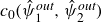 $c_0(\hat \psi _1^{\textit{out}},\hat \psi _2^{\textit{out}})$
for the concentration field shown in figure 10.
$c_0(\hat \psi _1^{\textit{out}},\hat \psi _2^{\textit{out}})$
for the concentration field shown in figure 10.
Mapping of the inlet concentration $c_0(\hat \psi _1,\hat \psi _2)$
shown in figure 10 to the outlet concentration
$c_0(\hat \psi _1,\hat \psi _2)$
shown in figure 10 to the outlet concentration $c_{\textit{out}}(\hat \psi _1,\hat \psi _2)\equiv c_0(\hat \psi ^{\textit{out}}_1,\hat \psi ^{\textit{out}}_2)$
. The resultant concentration profile is a direct result of the CS actions mediated by the separating streamsurfaces (indicated by green dashed lines) in the DFN.
$c_{\textit{out}}(\hat \psi _1,\hat \psi _2)\equiv c_0(\hat \psi ^{\textit{out}}_1,\hat \psi ^{\textit{out}}_2)$
. The resultant concentration profile is a direct result of the CS actions mediated by the separating streamsurfaces (indicated by green dashed lines) in the DFN.

In Appendix C, we show that under purely advective (non-dissipative) mixing, typical mixing measures such as concentration variance do not alter between $c_0$
and
$c_0$
and $c_{\textit{out}}$
. Instead we use a multi-scale mixing measure, the (squared) mix-norm
$c_{\textit{out}}$
. Instead we use a multi-scale mixing measure, the (squared) mix-norm $\varPhi ^2_{2\textit{-D}}$
(Mathew, Mezić & Petzold Reference Mathew, Mezić and Petzold2005), which robustly measures the degree of mixing by integrating over the scale-dependent concentration variance
$\varPhi ^2_{2\textit{-D}}$
(Mathew, Mezić & Petzold Reference Mathew, Mezić and Petzold2005), which robustly measures the degree of mixing by integrating over the scale-dependent concentration variance $\phi ^2_{2-D}(c_{\textit{out}},s)$
as
$\phi ^2_{2-D}(c_{\textit{out}},s)$
as
 \begin{equation} \varPhi ^2_{2\textit{-D}}\equiv \frac {1}{L}\int _0^L \phi ^2_{2\textit{-D}}(c_{\textit{out}},s)\,\text{d}s, \end{equation}
see Appendix C for details.
The 2-D concentration field $c_{\textit{out}}(\hat \psi _1,\hat \psi _2)$
and mixing measures
$c_{\textit{out}}(\hat \psi _1,\hat \psi _2)$
and mixing measures $\phi ^2_{2\textit{-D}}$
,
$\phi ^2_{2\textit{-D}}$
, $\varPhi ^2_{2\textit{-D}}$
provide a complete quantification of advective mixing over the fracture network. In Appendix C, we also show that a coarse-grained 1-D (
$\varPhi ^2_{2\textit{-D}}$
provide a complete quantification of advective mixing over the fracture network. In Appendix C, we also show that a coarse-grained 1-D ( $\hat \psi _1$
-only) representation also provides a highly accurate representation of advective mixing for
$\hat \psi _1$
-only) representation also provides a highly accurate representation of advective mixing for $\ell \ll L$
. In some instances, this coarse-grained representation is preferable to simplify visualisation of mixing and connect with observable concentration fields. Following Appendix C, a simple coarse-graining approach is employed which consists of averaging
$\ell \ll L$
. In some instances, this coarse-grained representation is preferable to simplify visualisation of mixing and connect with observable concentration fields. Following Appendix C, a simple coarse-graining approach is employed which consists of averaging $c_0$
and
$c_0$
and $c_{\textit{out}}$
with respect to
$c_{\textit{out}}$
with respect to $\hat \psi _2$
to yield
$\hat \psi _2$
to yield
 \begin{equation} c(\hat \psi _1)\equiv \int _0^1 c\left(\hat \psi _{1},\hat \psi _{2}\right)\,\text{d}\hat \psi _2,\quad c=c_0, c_{\textit{out}}, \end{equation}
where $c(\hat \psi _1)$
is differentiated from
$c(\hat \psi _1)$
is differentiated from $c(\hat \psi _1,\hat \psi _2)$
by its argument. Similarly, the global streamfunctions can be coarse-grained as
$c(\hat \psi _1,\hat \psi _2)$
by its argument. Similarly, the global streamfunctions can be coarse-grained as $\hat \psi _2^{\textit{out}})\mapsto \hat \psi _1^{\textit{out}}$
. Note that this averaging yields a simplified representation of advective mixing rather than a physical mixing process. The associated 1-D scale-dependent variance
$\hat \psi _2^{\textit{out}})\mapsto \hat \psi _1^{\textit{out}}$
. Note that this averaging yields a simplified representation of advective mixing rather than a physical mixing process. The associated 1-D scale-dependent variance $\phi ^2_{1\textit{-D}}(s)$
and mix-norm
$\phi ^2_{1\textit{-D}}(s)$
and mix-norm $\varPhi ^2_{1\textit{-D}}$
are defined analogously as their respective 2-D counterparts in (C5), (C6), and are related to the 2-D measures as
$\varPhi ^2_{1\textit{-D}}$
are defined analogously as their respective 2-D counterparts in (C5), (C6), and are related to the 2-D measures as
 \begin{align} \phi ^2_{1\textit{-D}}(s)= \begin{cases} 0\quad &0\lt s\leqslant \ell ,\\ \phi ^2_{2\textit{-D}}(s)\quad &\ell \lt s\leqslant L, \end{cases} && \varPhi ^2_{1\textit{-D}}=\varPhi ^2_{2\textit{-D},L}. \end{align}
Hence, the 1-D representation provides an accurate representation of mixing dynamics and the associated 1-D mixing measures $\phi ^2_{1\textit{-D}}$
,
$\phi ^2_{1\textit{-D}}$
, $\varPhi ^2_{1\textit{-D}}$
provide accurate estimates of their 2-D counterparts
$\varPhi ^2_{1\textit{-D}}$
provide accurate estimates of their 2-D counterparts $\phi ^2_{2\textit{-D}}$
,
$\phi ^2_{2\textit{-D}}$
, $\varPhi ^2_{2\textit{-D}}$
.
$\varPhi ^2_{2\textit{-D}}$
.
Many 2-D DFN models perform similar averaging on physical grounds, based on the assumption of complete mixing at fracture intersections. The validity of this assumption is quantified by the two Péclet numbers associated with the $\psi _1$
and
$\psi _1$
and $\psi _2$
coordinates, defined as
$\psi _2$
coordinates, defined as
 \begin{align} Pe_\|\equiv \frac {v_c L}{D_m}, && Pe_\bot \equiv \frac {v_c\ell }{D_m}, \end{align}
where $v_c$
is the characteristic velocity scale and
$v_c$
is the characteristic velocity scale and $D_m$
is the diffusion coefficient. Under such models, solute mixing is considered to be advection-dominated in the
$D_m$
is the diffusion coefficient. Under such models, solute mixing is considered to be advection-dominated in the $\psi _1$
direction (
$\psi _1$
direction ( $Pe_\|\gg 1$
) and diffusion-dominated in the
$Pe_\|\gg 1$
) and diffusion-dominated in the $\psi _2$
direction (
$\psi _2$
direction ( $Pe_\bot \ll 1$
), justifying the ‘well-mixed’ assumption commonly evoked at fracture intersections (Hyman & Jiménez-Martínez Reference Hyman and Jiménez-Martínez2018). However, such models cannot be readily generalised beyond these limits. Note that the averaging process (3.22) is not equivalent to such physical diffusion as it is applied as a post-processing step to the outlet concentration distribution
$Pe_\bot \ll 1$
), justifying the ‘well-mixed’ assumption commonly evoked at fracture intersections (Hyman & Jiménez-Martínez Reference Hyman and Jiménez-Martínez2018). However, such models cannot be readily generalised beyond these limits. Note that the averaging process (3.22) is not equivalent to such physical diffusion as it is applied as a post-processing step to the outlet concentration distribution $c_{\textit{out}}$
rather than a continual diffusion process throughout the fracture network.
$c_{\textit{out}}$
rather than a continual diffusion process throughout the fracture network.
(a,c) Isometric and (b,d) top views of test (a, b) DFN A and (c, d) DFN B.

4. Numerical simulations
4.1. Test DFNs and numerical method
The mixing measures $c_{\textit{out}}$
,
$c_{\textit{out}}$
, $\varPhi ^2_{1\textit{-D}}$
,
$\varPhi ^2_{1\textit{-D}}$
, $\phi ^2_{1\textit{-D}}(s)$
used to validate the advective mixing theory and associated mixing graph
$\phi ^2_{1\textit{-D}}(s)$
used to validate the advective mixing theory and associated mixing graph ${\mathcal{G}_M}$
by comparison with numerical simulations performed via the 2-D DFN simulation code DFN.lab (Le Goc et al. Reference Le Goc, Pinier, Darcel, Lavoine, Doolaeghe, de Simone, De Dreuzy and Davy2019). We consider two different test DFNs and test
${\mathcal{G}_M}$
by comparison with numerical simulations performed via the 2-D DFN simulation code DFN.lab (Le Goc et al. Reference Le Goc, Pinier, Darcel, Lavoine, Doolaeghe, de Simone, De Dreuzy and Davy2019). We consider two different test DFNs and test ${\mathcal{G}_M}$
under both the PWI (3.8) and PWS (3.9) variants of the intersection map
${\mathcal{G}_M}$
under both the PWI (3.8) and PWS (3.9) variants of the intersection map ${\mathcal{M}_I}$
. The first DFN considered (denoted DFN A) is shown in figures 12(a) and 12(b), and corresponds to the DFN shown in figure 1(b), which is less disordered than the second DFN considered (denoted DFN B) shown in figures 12(c) and 12(d). For both DFNs, flow in each fracture is modelled as a steady planar 2-D Darcy flow with uniform transmissivity. A prescribed pressure differential between the DFN inlets and outlets fixes the total volumetric flow at
${\mathcal{M}_I}$
. The first DFN considered (denoted DFN A) is shown in figures 12(a) and 12(b), and corresponds to the DFN shown in figure 1(b), which is less disordered than the second DFN considered (denoted DFN B) shown in figures 12(c) and 12(d). For both DFNs, flow in each fracture is modelled as a steady planar 2-D Darcy flow with uniform transmissivity. A prescribed pressure differential between the DFN inlets and outlets fixes the total volumetric flow at $Q=1$
. The inlet concentration is set to
$Q=1$
. The inlet concentration is set to $c_0(\hat \psi _1,\hat \psi _2)=0$
in one inlet fracture and
$c_0(\hat \psi _1,\hat \psi _2)=0$
in one inlet fracture and $c_0(\hat \psi _1,\hat \psi _2)=1$
in the other. The two outlets collect the discharge and all other boundaries are no-flux. DFN.lab is used to solve the flow and advect approximately
$c_0(\hat \psi _1,\hat \psi _2)=1$
in the other. The two outlets collect the discharge and all other boundaries are no-flux. DFN.lab is used to solve the flow and advect approximately $10^6$
streamlines that are seeded along the network inlets in a flux-weighted manner. Note that while a large number of streamlines are required to robustly test the accuracy of the mixing graph, only a small number of critical streamlines are required to quantify the mixing graph as described in § 3.5.
$10^6$
streamlines that are seeded along the network inlets in a flux-weighted manner. Note that while a large number of streamlines are required to robustly test the accuracy of the mixing graph, only a small number of critical streamlines are required to quantify the mixing graph as described in § 3.5.
4.2. Construction of mixing graph
${\mathcal{G}_M}$

From these numerical results, the topology of the mixing graph ${\mathcal{G}_M}$
is then determined by the connectivity (via streamlines) between fractures and intersections, and the edge weights of
${\mathcal{G}_M}$
is then determined by the connectivity (via streamlines) between fractures and intersections, and the edge weights of ${\mathcal{G}_M}$
are determined by the flow rates
${\mathcal{G}_M}$
are determined by the flow rates $Q_n$
between faces. The intersection
$Q_n$
between faces. The intersection ${\mathcal{M}_I}$
and fracture
${\mathcal{M}_I}$
and fracture ${\mathcal{M}_F}$
maps that operate respectively on intersection edges and fracture edges are determined from streamline routing. Note that for the PWI model (3.8), the intersection maps
${\mathcal{M}_F}$
maps that operate respectively on intersection edges and fracture edges are determined from streamline routing. Note that for the PWI model (3.8), the intersection maps ${\mathcal{M}_I}$
are determined solely from streamline routing data and the local
${\mathcal{M}_I}$
are determined solely from streamline routing data and the local $\psi _1$
streamfunction is invariant over an intersection. Conversely,
$\psi _1$
streamfunction is invariant over an intersection. Conversely, $\psi _1$
can vary under the PWS model (3.10), as is quantified by the flux distribution
$\psi _1$
can vary under the PWS model (3.10), as is quantified by the flux distribution $q_n$
over face
$q_n$
over face $f_n$
as detailed in Appendix B. Two-dimensional DFN models such as DFN.lab do not resolve the
$f_n$
as detailed in Appendix B. Two-dimensional DFN models such as DFN.lab do not resolve the $\psi _2$
coordinate, but instead perform random flux-weighted streamline routing at intersections, which is physically consistent with well-mixed conditions in the
$\psi _2$
coordinate, but instead perform random flux-weighted streamline routing at intersections, which is physically consistent with well-mixed conditions in the $\psi _2$
coordinate and the 1-D mixing representation outlined in Appendix C. Conversely, the PWI and PWS models for
$\psi _2$
coordinate and the 1-D mixing representation outlined in Appendix C. Conversely, the PWI and PWS models for ${\mathcal{G}_M}$
perform completely deterministic streamline routing based on the mixing maps
${\mathcal{G}_M}$
perform completely deterministic streamline routing based on the mixing maps ${\mathcal{M}_I}$
,
${\mathcal{M}_I}$
, ${\mathcal{M}_F}$
. We note that while the methods detailed in § 3 allow both
${\mathcal{M}_F}$
. We note that while the methods detailed in § 3 allow both $\psi _1$
and
$\psi _1$
and $\psi _2$
to be resolved, in this section we only compare 1-D mixing results between DFN.lab and the mixing graph
$\psi _2$
to be resolved, in this section we only compare 1-D mixing results between DFN.lab and the mixing graph ${\mathcal{G}_M}$
.
${\mathcal{G}_M}$
.
Development and application of the mixing graph ${\mathcal{G}_M}$
and the mixing maps
${\mathcal{G}_M}$
and the mixing maps ${\mathcal{M}_I}$
(PWI model) and
${\mathcal{M}_I}$
(PWI model) and ${\mathcal{M}_F}$
for DFN A results in the 2-D concentration fields shown in figure 10. This clearly illustrates the impact of intersection and fracture mixing mechanisms upon the local concentration field
${\mathcal{M}_F}$
for DFN A results in the 2-D concentration fields shown in figure 10. This clearly illustrates the impact of intersection and fracture mixing mechanisms upon the local concentration field $c_n(\psi _{1,n},\psi _{2,n})$
at each face
$c_n(\psi _{1,n},\psi _{2,n})$
at each face $f_n$
, and the corresponding 1-D mixing plot is shown in figure 18(d).
$f_n$
, and the corresponding 1-D mixing plot is shown in figure 18(d).
4.3. Comparison of advective mixing in test DFNs
Figure 13 compares the 1-D mixing plots (see details in Appendix D) for both test DFNs generated by DFN.lab and ${\mathcal{G}_M}$
under both the PWI and PWS models. Figure 13(a) and table 1 show that the PWI model fairly accurately captures the mixing dynamics generated by DFN.lab for DFN A in terms of both the outlet concentration distribution
${\mathcal{G}_M}$
under both the PWI and PWS models. Figure 13(a) and table 1 show that the PWI model fairly accurately captures the mixing dynamics generated by DFN.lab for DFN A in terms of both the outlet concentration distribution $c_{\textit{out}}(\hat \psi _1)$
and mapping
$c_{\textit{out}}(\hat \psi _1)$
and mapping $\hat \psi _1\mapsto \hat \psi _1^{\textit{out}}$
, although some minor differences are apparent. In these plots, CS of fluid elements is clearly shown by the cut and shuffled 1-D lines in the
$\hat \psi _1\mapsto \hat \psi _1^{\textit{out}}$
, although some minor differences are apparent. In these plots, CS of fluid elements is clearly shown by the cut and shuffled 1-D lines in the $\hat \psi _1-\hat \psi _1^{\textit{out}}$
plane, as well as the impact of intersection mixing which dilutes the 1-D outlet concentration field as
$\hat \psi _1-\hat \psi _1^{\textit{out}}$
plane, as well as the impact of intersection mixing which dilutes the 1-D outlet concentration field as $0\lt c_{\textit{out}}(\hat \psi _1)\lt 1$
. An inherent property of the PWI model is that it produces straight lines in the
$0\lt c_{\textit{out}}(\hat \psi _1)\lt 1$
. An inherent property of the PWI model is that it produces straight lines in the $\hat \psi _1-\hat \psi _1^{\textit{out}}$
plane as fluid parcels only undergo CS in the
$\hat \psi _1-\hat \psi _1^{\textit{out}}$
plane as fluid parcels only undergo CS in the $\psi _1$
coordinate without deformation (stretching or compression); hence, the mapping
$\psi _1$
coordinate without deformation (stretching or compression); hence, the mapping $\hat \psi _1\mapsto \hat \psi _1^{\textit{out}}$
is piecewise linear. Conversely, the DFN.lab results show some evidence of streamline deformation, as indicated by the slight curvature of lines in the
$\hat \psi _1\mapsto \hat \psi _1^{\textit{out}}$
is piecewise linear. Conversely, the DFN.lab results show some evidence of streamline deformation, as indicated by the slight curvature of lines in the $\hat \psi _1-\hat \psi _1^{\textit{out}}$
plane.
$\hat \psi _1-\hat \psi _1^{\textit{out}}$
plane.
Comparison of the 1-D mixing plots for (a, b) DFN A and (c,d) DFN B generated by DFN.lab and ${\mathcal{G}_M}$
under the (a,c) PWI and (b,d) PWS models. Colour bars denote inlet
${\mathcal{G}_M}$
under the (a,c) PWI and (b,d) PWS models. Colour bars denote inlet $c_0(\hat \psi _1)$
and outlet
$c_0(\hat \psi _1)$
and outlet $c_{\textit{out}}(\hat \psi _1)$
concentration distributions, and shaded bands indicate overlap regions of intersection mixing leading to
$c_{\textit{out}}(\hat \psi _1)$
concentration distributions, and shaded bands indicate overlap regions of intersection mixing leading to $0\lt c_{\textit{out}}(\hat \psi _1)\lt 1$
.
$0\lt c_{\textit{out}}(\hat \psi _1)\lt 1$
.

Figure 13(b) and table 1 shows that for DFN A, the PWS model predicts the outlet concentration $c_{\textit{out}}(\hat \psi _1)$
and streamfunctions
$c_{\textit{out}}(\hat \psi _1)$
and streamfunctions $\hat \psi _1^{\textit{out}}$
almost exactly due to resolution of fluid deformation during advective mixing. The difference between the PWI and PWS models is more pronounced for DFN B, consistent with the more disordered nature of this DFN. Figure 13(c) shows a significant level of discrepancy between the PWI model and the DFN.lab results, whereas the PWS model (figure 13
d) accurately reproduces the mixing dynamics generated by DFN.lab. As many fracture networks typically exhibit a much larger level of disorder than DFN B, the impact of fluid deformation upon advective mixing is likely to be more pronounced than that indicated in figures 13(c) and 13(d).
$\hat \psi _1^{\textit{out}}$
almost exactly due to resolution of fluid deformation during advective mixing. The difference between the PWI and PWS models is more pronounced for DFN B, consistent with the more disordered nature of this DFN. Figure 13(c) shows a significant level of discrepancy between the PWI model and the DFN.lab results, whereas the PWS model (figure 13
d) accurately reproduces the mixing dynamics generated by DFN.lab. As many fracture networks typically exhibit a much larger level of disorder than DFN B, the impact of fluid deformation upon advective mixing is likely to be more pronounced than that indicated in figures 13(c) and 13(d).
Comparison of 1-D mix-norm values $\varPhi ^2_{1\textit{-D}}$
for the test DFNs between the DFN.lab results and the PWI and PWS models for
$\varPhi ^2_{1\textit{-D}}$
for the test DFNs between the DFN.lab results and the PWI and PWS models for ${\mathcal{G}_M}$
.
${\mathcal{G}_M}$
.

Figure 14 shows that that while the PWS model results very closely match the DFN.lab results for both test DFNs, the PWI model results slightly deviate at small to intermediate scales for DFN A and in a more pronounced fashion for DFN B. This is consistent with the $\varPhi ^2_{1\textit{-D}}$
values in table 1, which indicates that the PWI model for DFN A and B incurs respective mix-norm errors of 1.4 % and 10.5 %, whereas the PWS model is highly accurate. The excellent level of agreement between DFN.lab and the PWS model confirms that advective mixing in fracture networks follows a PWS discontinuous mixing process.
$\varPhi ^2_{1\textit{-D}}$
values in table 1, which indicates that the PWI model for DFN A and B incurs respective mix-norm errors of 1.4 % and 10.5 %, whereas the PWS model is highly accurate. The excellent level of agreement between DFN.lab and the PWS model confirms that advective mixing in fracture networks follows a PWS discontinuous mixing process.
Comparison of multi-scale variance $\phi ^2_{1\textit{-D}}(s)$
for (a) DFN A and (b) DFN B between DFN.lab results (blue dots) and the PWS (orange crosses) and PWI (grey crosses) models for
$\phi ^2_{1\textit{-D}}(s)$
for (a) DFN A and (b) DFN B between DFN.lab results (blue dots) and the PWS (orange crosses) and PWI (grey crosses) models for ${\mathcal{G}_M}$
.
${\mathcal{G}_M}$
.

4.4. Advective mixing in iterated fracture networks
To highlight the utility of the graph-based approach, we also consider iterated mixing in DFN B, where the outlet concentration distribution $c_{\textit{out}}(\hat \psi _1)$
for one iteration of the network forms the inlet concentration distribution
$c_{\textit{out}}(\hat \psi _1)$
for one iteration of the network forms the inlet concentration distribution $c_0(\hat \psi _1)$
for the following iteration. The 1-D mixing plots in figure 15 show that under both the PWI and PWS models, this DFN exhibits rapid and complete mixing with increasing iteration number
$c_0(\hat \psi _1)$
for the following iteration. The 1-D mixing plots in figure 15 show that under both the PWI and PWS models, this DFN exhibits rapid and complete mixing with increasing iteration number $n$
, where the outlet concentration
$n$
, where the outlet concentration $c_{\textit{out}}\rightarrow 1/2$
as
$c_{\textit{out}}\rightarrow 1/2$
as $n\rightarrow \infty$
. Similarly, figure 16 shows that the 1-D mix-norm
$n\rightarrow \infty$
. Similarly, figure 16 shows that the 1-D mix-norm $\varPhi ^2_{1\textit{-D}}(n)$
for both models converges towards zero with
$\varPhi ^2_{1\textit{-D}}(n)$
for both models converges towards zero with $n$
as a power-law (
$n$
as a power-law (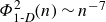 $\varPhi ^2_{1\textit{-D}}(n)\sim n^{-7}$
), reflecting weak ergodic mixing (algebraic decay) of the PWI and PWS transforms. Figure 16 also shows that
$\varPhi ^2_{1\textit{-D}}(n)\sim n^{-7}$
), reflecting weak ergodic mixing (algebraic decay) of the PWI and PWS transforms. Figure 16 also shows that $\varPhi ^2_{1\textit{-D}}(n)$
is quite similar between the PWI and the PWS models, suggesting that although the PWI model does not resolve the detailed mixing dynamics, this has minimal impact on quantifying mixing in larger fracture networks.
$\varPhi ^2_{1\textit{-D}}(n)$
is quite similar between the PWI and the PWS models, suggesting that although the PWI model does not resolve the detailed mixing dynamics, this has minimal impact on quantifying mixing in larger fracture networks.
Evolution of 1-D mixing plots for iterated mixing in DFN B under the (a–d) PWS and (e–h) PWI mixing graph representations after $n=2$
,
$n=2$
, $n=4$
,
$n=4$
, $n=8$
and
$n=8$
and $n=16$
iterations.).
$n=16$
iterations.).

Decay of 1-D mix-norm $\varPhi ^2_{1\textit{-D}}(n)$
as a function of iteration number
$\varPhi ^2_{1\textit{-D}}(n)$
as a function of iteration number $n$
for the orthogonal DFN under the PWS and PWI models.
$n$
for the orthogonal DFN under the PWS and PWI models.

5. Conclusions
In this study, we identify the fundamental mechanisms controlling advective mixing in three-dimensional (3-D) DFNs and leverage these insights to develop a parsimonious, graph-based representation of advective mixing. We examine the Lagrangian kinematics of 3-D DFNs under steady, isotropic Darcy flow. Although this assumption precludes chaotic advection, such effects are shown to be negligible due to the highly constrained geometry of fracture networks. Instead, the intrinsic topological complexity of fracture networks gives rise to stagnation points and critical lines that regulate mixing through streamline routing.
We show that mixing is governed by discontinuous mixing, whereby fluid elements undergo cutting and shuffling (CS) as streamlines are routed through fractures and their intersections. We identify two distinct mechanisms: fracture mixing and intersection mixing, which respectively control mixing within individual fractures and at their intersections. These mechanisms operate over widely separated length scales: fracture mixing cuts and shuffles fluid elements at the fracture scale $L$
, whereas intersection mixing acts at the much smaller aperture scale
$L$
, whereas intersection mixing acts at the much smaller aperture scale $\ell$
, with
$\ell$
, with $\ell \ll L$
. This CS process is illustrated in figure 11, which shows how the tracer concentration field
$\ell \ll L$
. This CS process is illustrated in figure 11, which shows how the tracer concentration field $c_0$
over the inlets to the DFN (figure 1
b,c) is mapped to the outlet concentration distribution via cutting and shuffling of fluid elements.
$c_0$
over the inlets to the DFN (figure 1
b,c) is mapped to the outlet concentration distribution via cutting and shuffling of fluid elements.
Hence, the mixing dynamics in DFNs differs fundamentally from granular media, where mixing arises purely through continuous stretching and folding (SF) of fluid elements, and also from 3-D porous networks, which exhibit a combination of continuous (SF) and discontinuous cutting and shuffling (CS) dynamics (Lester et al. Reference Lester, Heyman, Méheust and Le Borgne2025a ). As the geometry of porous materials becomes increasingly constrained – from granular media to pore networks to fractured networks – the dominant mixing behaviour correspondingly transitions from continuous (SF), to mixed (SF/CS) and ultimately to predominantly discontinuous (CS) dynamics.
A streamfunction coordinate system is used to construct intersection ${\mathcal{M}_I}$
and fracture
${\mathcal{M}_I}$
and fracture ${\mathcal{M}_F}$
mixing maps that compactly encode advective mixing. We consider two variants of the intersection map
${\mathcal{M}_F}$
mixing maps that compactly encode advective mixing. We consider two variants of the intersection map ${\mathcal{M}_I}$
: a piecewise smooth (PWS) model that accounts for fluid deformation arising from velocity fluctuations, and a piecewise isometric (PWI) model that neglects this effect. These maps are embedded within a mixing graph
${\mathcal{M}_I}$
: a piecewise smooth (PWS) model that accounts for fluid deformation arising from velocity fluctuations, and a piecewise isometric (PWI) model that neglects this effect. These maps are embedded within a mixing graph ${\mathcal{G}_M}$
– an enriched extension of the intersection graph
${\mathcal{G}_M}$
– an enriched extension of the intersection graph ${\mathcal{G}_I}$
(Ahuja et al. Reference Ahuja, Magnanti and Orlin1993) – that represents the topology of connected fractures and intersections. The mixing graph
${\mathcal{G}_I}$
(Ahuja et al. Reference Ahuja, Magnanti and Orlin1993) – that represents the topology of connected fractures and intersections. The mixing graph ${\mathcal{G}_M}$
enables efficient streamline routing through the fracture network and predictive modelling of advective mixing in DFNs. Via CS, the PWI and PWS models both encode mixing interfaces that grow linearly from intersection to intersection in the network, which is consistent with the algebraic growth rates observed by Hallack et al. (Reference Hallack, Bolster, Hyman, Sweeney and Viswanathan2025).
${\mathcal{G}_M}$
enables efficient streamline routing through the fracture network and predictive modelling of advective mixing in DFNs. Via CS, the PWI and PWS models both encode mixing interfaces that grow linearly from intersection to intersection in the network, which is consistent with the algebraic growth rates observed by Hallack et al. (Reference Hallack, Bolster, Hyman, Sweeney and Viswanathan2025).
The PWS and PWI formulations of the mixing graph ${\mathcal{G}_M}$
are evaluated against numerical simulations of flow and transport in two test DFNs using the DFN.lab software package. The PWS model reproduces the mixing dynamics with high accuracy (
${\mathcal{G}_M}$
are evaluated against numerical simulations of flow and transport in two test DFNs using the DFN.lab software package. The PWS model reproduces the mixing dynamics with high accuracy ( $\mathcal{O}(10^{-5})$
), confirming that the underlying discontinuous mixing is piecewise smooth and characterised by cutting and shuffling coupled with fluctuating fluid stretching. In contrast, the PWI mixing graph representation yields small errors
$\mathcal{O}(10^{-5})$
), confirming that the underlying discontinuous mixing is piecewise smooth and characterised by cutting and shuffling coupled with fluctuating fluid stretching. In contrast, the PWI mixing graph representation yields small errors $(\mathcal{O}(10^{-2}))$
for one test DFN and larger errors
$(\mathcal{O}(10^{-2}))$
for one test DFN and larger errors $(\mathcal{O}(10^{-1}))$
for a more disordered network, indicating that structural disorder promotes fluid deformation. Despite these discrepancies at the local scale, the PWS and PWI models exhibit similar mixing behaviour under iterated mixing representative of larger fracture networks. We also note that a simple modification of the PWI method provides an excellent approximation of the PWS method; although beyond the scope of thus study, this method shall be explored further in the future.
$(\mathcal{O}(10^{-1}))$
for a more disordered network, indicating that structural disorder promotes fluid deformation. Despite these discrepancies at the local scale, the PWS and PWI models exhibit similar mixing behaviour under iterated mixing representative of larger fracture networks. We also note that a simple modification of the PWI method provides an excellent approximation of the PWS method; although beyond the scope of thus study, this method shall be explored further in the future.
This convergence suggests that deformation-induced effects may become negligible at larger scales. Overall, we find that although advective mixing in fracture networks is only weakly ergodic, it remains efficient due to interplay of fine-scale intersection mixing at length scale $\ell$
and fracture-scale mixing at length scale
$\ell$
and fracture-scale mixing at length scale $L$
efficiently which brings fluid elements from disparate regions of the network into contact. Together, these complementary mechanisms drive rapid advective mixing in 3-D DFNs.
$L$
efficiently which brings fluid elements from disparate regions of the network into contact. Together, these complementary mechanisms drive rapid advective mixing in 3-D DFNs.
The mixing graph framework readily supports upscaled analytic and numerical models of mixing and transport in large fracture networks, for example, through stochastic formulations or random graphs conditioned on laboratory or field observations. The key DFN properties that govern advective mixing are (i) the distribution of fluid fluxes between fractures and their intersections and (ii) the network topology defined by these connected elements. As the distribution of fluxes at fractures and intersections control the advective mixing process, fracture networks with more uniform flux distributions (given the same topology) generate more efficient mixing and highly non-uniform flux distributions lead to ‘short-circuiting’ involving inefficient CS actions that are not even distributed throughout $\psi _1$
,
$\psi _1$
, $\psi _2$
. The quantification of these properties in large-scale fracture networks would then provide a solid foundation for the development of predictive theories of advective mixing, as well as efficient numerical methods for simulation of transport and mixing.
$\psi _2$
. The quantification of these properties in large-scale fracture networks would then provide a solid foundation for the development of predictive theories of advective mixing, as well as efficient numerical methods for simulation of transport and mixing.
The advent of such tools and insights establishes a rigorous framework for future studies of fluid-borne processes in fractured media. As shown in figures 10 and 11, advective mixing in 3-D DFNs is controlled by separating streamsurfaces that encode the series of CS actions that evolve the 2-D concentration distribution $c_n(\psi _{1,n},\psi _{2,n})$
at each face
$c_n(\psi _{1,n},\psi _{2,n})$
at each face $f_n$
in the network. While the mixing maps
$f_n$
in the network. While the mixing maps ${\mathcal{M}_I}$
,
${\mathcal{M}_I}$
, ${\mathcal{M}_F}$
can be used to advect arbitrary streamlines, such that the streamfunctions are mapped from face to face throughout the network as
${\mathcal{M}_F}$
can be used to advect arbitrary streamlines, such that the streamfunctions are mapped from face to face throughout the network as $(\psi _{1,n},\psi _{2,n}) \xrightarrow{{\mathcal{M}_I}, {\mathcal{M}_F}} (\psi _{1,m},\psi _{2,m})$
, they can also be employed to resolve these separating streamsurfaces and construct advective maps
$(\psi _{1,n},\psi _{2,n}) \xrightarrow{{\mathcal{M}_I}, {\mathcal{M}_F}} (\psi _{1,m},\psi _{2,m})$
, they can also be employed to resolve these separating streamsurfaces and construct advective maps ${\mathcal{A}_I}$
,
${\mathcal{A}_I}$
, ${\mathcal{A}_F}$
that propagate the local concentration field
${\mathcal{A}_F}$
that propagate the local concentration field $c_n$
throughout the network as
$c_n$
throughout the network as $c_n \xrightarrow{{\mathcal{A}_I}, {\mathcal{A}_F}} c_m$
. This framework not only provides an efficient means of propagating the concentration field under advective mixing, but also establishes a foundation for modelling time-dependent processes such as solute mixing and dispersion, chemical reactions and biological activity.
$c_n \xrightarrow{{\mathcal{A}_I}, {\mathcal{A}_F}} c_m$
. This framework not only provides an efficient means of propagating the concentration field under advective mixing, but also establishes a foundation for modelling time-dependent processes such as solute mixing and dispersion, chemical reactions and biological activity.
For example, given the residence-time distribution $\tau _n$
over each fracture
$\tau _n$
over each fracture $n$
in the DFN (assuming negligible travel time
$n$
in the DFN (assuming negligible travel time $\tau _n=0$
over an intersection), then the distribution of Lagrangian travel times
$\tau _n=0$
over an intersection), then the distribution of Lagrangian travel times $t_n(\psi _{1,n},\psi _{2,n})=\sum _{i=1}^n\tau _i$
over each face generates the temporal maps
$t_n(\psi _{1,n},\psi _{2,n})=\sum _{i=1}^n\tau _i$
over each face generates the temporal maps $\mathcal{T}_F$
,
$\mathcal{T}_F$
, $\mathcal{T}_I=I$
that propagate
$\mathcal{T}_I=I$
that propagate $t_n$
through the network. For solute mixing, methods that combine CS and diffusion processes (Ashwin, Nicol & Kirkby Reference Ashwin, Nicol and Kirkby2002; Kreczak Reference Kreczak2019) can be used to generate diffusive maps
$t_n$
through the network. For solute mixing, methods that combine CS and diffusion processes (Ashwin, Nicol & Kirkby Reference Ashwin, Nicol and Kirkby2002; Kreczak Reference Kreczak2019) can be used to generate diffusive maps $\mathcal{D}_F=\mathcal{D}_F({\mathcal{A}_F},\mathcal{T}_F)$
,
$\mathcal{D}_F=\mathcal{D}_F({\mathcal{A}_F},\mathcal{T}_F)$
, $\mathcal{D}_I={\mathcal{A}_I}$
that propagate the solute concentration
$\mathcal{D}_I={\mathcal{A}_I}$
that propagate the solute concentration $c_n$
throughout the network. This allows solute mixing in intersections to be properly resolved for finite transverse Péclet numbers (
$c_n$
throughout the network. This allows solute mixing in intersections to be properly resolved for finite transverse Péclet numbers ( $Pe_\bot$
in (3.24)), without resorting to extreme approximations such as complete mixing or streamline routing at intersections. Conversely, solute mixing in fractures is governed by the longitudinal Péclet number (
$Pe_\bot$
in (3.24)), without resorting to extreme approximations such as complete mixing or streamline routing at intersections. Conversely, solute mixing in fractures is governed by the longitudinal Péclet number ( $Pe_{||}$
), where
$Pe_{||}$
), where $Pe_{||}=L/\ell \,Pe_\bot$
. Similar approaches can also be developed for longitudinal and transverse dispersion, and reactive transport.
$Pe_{||}=L/\ell \,Pe_\bot$
. Similar approaches can also be developed for longitudinal and transverse dispersion, and reactive transport.
Acknowledgements
Views and opinions expressed are those of the author(s) only and do not necessarily reflect those of the European Union or the European Research Council Executive Agency. Neither the European Union nor the granting authority can be held responsible for them. T.L.B. and J.H. also acknowledge Campus France. The authors gratefully acknowledge the Fractory (a joint laboratory of Itasca, the CNRS and the University of Rennes) for making DFN.lab available for this study.
Funding
This research was funded by the European Union under the grants MSCA COFUND 101034328 (REDI) and ERC 101042466 (CHORUS). We also acknowledge PHC FASIC (CHAOSTRALIA).
Data availability statement
The numerical codes and relevant data are available at https://gitlab.com/stefanoascione93/dfn_mixing.
Declaration of interests
The authors report no conflict of interest.
Appendix A. Chaotic advection in fracture networks
A.1. Estimation of Lyapunov exponent in fracture networks
Lester et al. (Reference Lester, Heyman, Méheust and Le Borgne2025a
) show that the Lyapunov exponent $\hat {\lambda }_\infty$
in ordered pore networks is controlled by the orientation angles
$\hat {\lambda }_\infty$
in ordered pore networks is controlled by the orientation angles $\delta$
,
$\delta$
, $\Delta$
between manifolds as
$\Delta$
between manifolds as
 \begin{equation} \hat {\lambda }_\infty (\delta ,\varDelta )=\max (\ln (|\xi |\pm \sqrt {\xi ^2-1}),0),\quad \xi =\frac {9}{8}\cos \delta -\frac {1}{8}\cos (2\Delta +\delta ), \end{equation}
with $\delta \in [-\pi ,\pi ]$
,
$\delta \in [-\pi ,\pi ]$
, $\Delta \in [-\pi ,\pi ]$
. For random pore networks with
$\Delta \in [-\pi ,\pi ]$
. For random pore networks with $\delta$
,
$\delta$
, $\varDelta$
both uniformly distributed between
$\varDelta$
both uniformly distributed between $-\pi$
and
$-\pi$
and $\pi$
, the average Lyapunov exponent is given by the ensemble average
$\pi$
, the average Lyapunov exponent is given by the ensemble average
 \begin{equation} \lambda _\infty \equiv \frac {1}{4\pi ^2}\int _{-\pi }^\pi \int _{-\pi }^\pi \hat {\lambda }_\infty (\delta ,\varDelta )\,\text{d}\delta \,\text{d}\Delta \approx 0.1178. \end{equation}
For fracture networks, these angles are constrained as $\delta \in [-\alpha ,\alpha ]$
,
$\delta \in [-\alpha ,\alpha ]$
, $\Delta \in [-\alpha ,\alpha ]$
, where
$\Delta \in [-\alpha ,\alpha ]$
, where $\alpha =\arctan (\ell /L)\approx \ell /L\ll 1$
. Assuming these angles are uniformly distributed in fracture networks within these limits, then
$\alpha =\arctan (\ell /L)\approx \ell /L\ll 1$
. Assuming these angles are uniformly distributed in fracture networks within these limits, then $\hat \lambda _\infty$
is symmetric about
$\hat \lambda _\infty$
is symmetric about $\delta =0$
,
$\delta =0$
, $\varDelta =0$
,
$\varDelta =0$
,
 \begin{equation} \lambda _\infty \equiv \frac {1}{2\alpha ^2}\int _{0}^\alpha \int _{-\alpha }^\alpha \hat {\lambda }_\infty (\delta ,\varDelta )\,\text{d}\delta \,\text{d}\Delta . \end{equation}
As $\hat \lambda _\infty \gt 0$
for
$\hat \lambda _\infty \gt 0$
for $\varDelta \gt 0$
and
$\varDelta \gt 0$
and $-\varDelta /2\lt \delta \lt \varDelta$
, then to leading order, the
$-\varDelta /2\lt \delta \lt \varDelta$
, then to leading order, the $\delta$
integral in (A3) can be approximated by Simpson’s rule as
$\delta$
integral in (A3) can be approximated by Simpson’s rule as
 \begin{equation} \int _{-\alpha }^\alpha \hat \lambda _\infty (\delta ,\varDelta )\,\text{d}\alpha =\int _{-\Delta /2}^\Delta \hat \lambda _\infty (\delta ,\varDelta )\,\text{d}\alpha \approx \frac {3\Delta }{4}\frac {4}{3}\hat \lambda _\infty (\delta =\Delta /4,\Delta )\approx \frac {3}{4}\Delta ^2+\mathcal{O}(\Delta ^3). \end{equation}
Integrating with respect $\varDelta$
over
$\varDelta$
over $\varDelta \in [0,\alpha ]$
then yields
$\varDelta \in [0,\alpha ]$
then yields
 \begin{equation} \lambda _\infty \approx \frac {1}{2\alpha ^2}\frac {\alpha ^3}{4}=\frac {\alpha }{8}\approx \frac {1}{8}\frac {\ell }{L}\ll 1. \end{equation}
A.2. Generation of helicity density in fracture networks
We show that under Stokes flow, the helicity density is generated at fracture boundaries by consideration of the helicity density evolution equation (Moffatt Reference Moffatt1969) that arises from the incompressible Navier–Stokes and vorticity equations
 \begin{align} \frac {{\textrm D}\boldsymbol{v}}{{\textrm D}t}&=-\frac {1}{\rho }\boldsymbol{\nabla }p+\nu \boldsymbol{\nabla} ^2\boldsymbol{v},\quad \boldsymbol{\nabla }\boldsymbol{\cdot }\boldsymbol{v}=0, \end{align}
 \begin{align} \frac {{\textrm D}\boldsymbol \omega }{{\textrm D}t}&=\boldsymbol \omega \boldsymbol{\cdot }\boldsymbol{\nabla }\boldsymbol{v}+\nu \boldsymbol{\nabla} ^2\boldsymbol \omega ,\quad \boldsymbol{\nabla }\boldsymbol{\cdot }\boldsymbol \omega =0, \end{align}
 \begin{equation} \frac {{\textrm D}h}{{\textrm D}t}=\frac {{\textrm D}\boldsymbol{v}}{{\textrm D}t}\boldsymbol{\cdot }\boldsymbol \omega +\frac {{\textrm D}\boldsymbol \omega }{{\textrm D}t}\boldsymbol{\cdot }\boldsymbol{v}=\nu \big [\boldsymbol{v}\boldsymbol{\cdot }\boldsymbol{\nabla} ^2\boldsymbol \omega +\boldsymbol \omega \boldsymbol{\cdot }\boldsymbol{\nabla} ^2\boldsymbol{v}\big ]+\boldsymbol{\nabla }\boldsymbol{\cdot }\left [\boldsymbol \omega \left (-\frac {p}{\rho }+\frac {1}{2}v^2\right )\right ], \end{equation}
where the first term on the right-hand side represents viscous helicity dissipation and the second term on the right-hand side represents conservative helicity density flux. From (A7), under Stokes flow the vorticity vector satisfies $\nabla^2\boldsymbol\omega=\boldsymbol{0}$
, hence vorticity is only generated at the no-slip domain boundaries and then it diffuses into the bulk. From (A8), vorticity in the bulk can generate non-zero helicity via the first term on the right-hand of (A8) (Moffatt Reference Moffatt1969).
$\nabla^2\boldsymbol\omega=\boldsymbol{0}$
, hence vorticity is only generated at the no-slip domain boundaries and then it diffuses into the bulk. From (A8), vorticity in the bulk can generate non-zero helicity via the first term on the right-hand of (A8) (Moffatt Reference Moffatt1969).
Appendix B. Quantification of mixing maps
${\mathcal{M}_I}$
,
${\mathcal{M}_F}$


B.1. Quantification of the intersection mixing map
${\mathcal{M}_I}$

B.1.1. Differentiation of PWI and PWS transforms
The difference between the PWI and PWS transforms can be clearly demonstrated for the case of flow through a T-shaped intersection such as the $\hat \psi _1$
-streamsurface shown in figure 4(e). Under the assumption of zero flow along the intersection, streamlines are confined to
$\hat \psi _1$
-streamsurface shown in figure 4(e). Under the assumption of zero flow along the intersection, streamlines are confined to $\hat \psi _1$
-streamsurfaces that are also planes of constant
$\hat \psi _1$
-streamsurfaces that are also planes of constant $x_1$
. Denoting the faces in figure 4(e) as
$x_1$
. Denoting the faces in figure 4(e) as $f_1\equiv f_1^i$
,
$f_1\equiv f_1^i$
, $f_2\equiv f_1^o$
,
$f_2\equiv f_1^o$
, $f_3\equiv f_2^o$
, an overall flux balance gives
$f_3\equiv f_2^o$
, an overall flux balance gives $Q_1=Q_2+Q_3$
. An areal flux balance within a
$Q_1=Q_2+Q_3$
. An areal flux balance within a $\hat \psi _1$
-streamsurface also means that the areal fluxes
$\hat \psi _1$
-streamsurface also means that the areal fluxes $q_n(x_1)$
(3.7) are related as
$q_n(x_1)$
(3.7) are related as
 \begin{align} q_1(x_1)=&\int _0^1||\boldsymbol{v}_1||\,\text{d}\psi _{2,1}=Q_1\boldsymbol{\nabla }\psi _{1,1}, \end{align}
 \begin{align} q_2(x_1)=&\int _0^1||\boldsymbol{v}_2||\,\text{d}\psi _{2,2}=Q_2\boldsymbol{\nabla }\psi _{1,2}=\int _0^{\psi _{2,1}^\star }||\boldsymbol{v}_1||\,\text{d}\psi _{2,1}=\psi _{2,1}^\star Q_1\boldsymbol{\nabla }\psi _{1,1}=\psi _{2,1}^\star q_1(x_1), \end{align}
 \begin{align} q_3(x_1) &=\int _0^1||\boldsymbol{v}_3||\,\text{d}\psi _{2,3}=Q_3\boldsymbol{\nabla }\psi _{1,3}=\int _{\psi _{2,1}^\star }^1||\boldsymbol{v}_1||\,\text{d}\psi _{2,1}=(1-\psi _{2,1}^\star ) Q_1\boldsymbol{\nabla }\psi _{1,1} \nonumber\\ & =(1-\psi _{2,1}^\star ) q_1(x_1), \end{align}
where $\psi _{2,1}^\star$
is the
$\psi _{2,1}^\star$
is the $\psi _{2,1}$
value of the separating streamline in the inlet. Extending this relationship along the entire longitudinal coordinate
$\psi _{2,1}$
value of the separating streamline in the inlet. Extending this relationship along the entire longitudinal coordinate $x_1$
of the intersection,
$x_1$
of the intersection, $\psi _{2,1}^\star (x_1)$
varies with
$\psi _{2,1}^\star (x_1)$
varies with $x_1$
as
$x_1$
as
 \begin{equation} \psi _{2,1}^\star (x_1)=\frac {q_2(x_1)}{q_1(x_1)}=1-\frac {q_3(x_1)}{q_1(x_1)}, \end{equation}
and hence $\psi _{2,1}^\star (x_1)$
is invariant along the intersection if the ratio of areal fluxes is constant throughout.
$\psi _{2,1}^\star (x_1)$
is invariant along the intersection if the ratio of areal fluxes is constant throughout.
As only critical features such as separating streamlines control streamline routing and advective mixing, the condition $q_1(x_1)/q_2(x_1)=$
const. means that intersection mixing does not vary with
$q_1(x_1)/q_2(x_1)=$
const. means that intersection mixing does not vary with $x_1$
and the separating streamline only depends upon the volumetric fluxes as
$x_1$
and the separating streamline only depends upon the volumetric fluxes as
 \begin{equation} \psi _{2,1}^\star =\frac {Q_2}{Q_1}=1-\frac {Q_3}{Q_1}. \end{equation}
Thus, intersection mixing may be determined completely from the volumetric fluxes $Q_1$
,
$Q_1$
, $Q_2$
,
$Q_2$
, $Q_3$
. This formulation (B5) is consistent with the PWI transform, where stretching due to velocity fluctuations is negligible, whereas the variable flux case (B4) is consistent with the PWS transform. As the local
$Q_3$
. This formulation (B5) is consistent with the PWI transform, where stretching due to velocity fluctuations is negligible, whereas the variable flux case (B4) is consistent with the PWS transform. As the local $\psi _{1,n}$
streamfunction also depends upon the areal fluxes, if
$\psi _{1,n}$
streamfunction also depends upon the areal fluxes, if $q_1(x_1)/q_2(x_1)=$
const., then these are equivalent as
$q_1(x_1)/q_2(x_1)=$
const., then these are equivalent as
 \begin{equation} \psi _{1,1}(x_1)=\frac {1}{Q_1}\int _0^{x_1}q_1(x_1^\prime )\,\text{d}x_1^\prime =\frac {1}{Q_2}\int _0^{x_1}q_2(x_1^\prime )\,\text{d}x_1^\prime =\psi _{1,2}(x_1), \end{equation}
hence, all the $\psi _{1,n}$
streamfunctions are invariant over an intersection under the PWI model.
$\psi _{1,n}$
streamfunctions are invariant over an intersection under the PWI model.
These concepts can be readily generalised to the various intersection and streamline topologies shown in figure 4, leading to the result that the intersection mixing dynamics along $x_1$
is also invariant if the ratio of areal fluxes
$x_1$
is also invariant if the ratio of areal fluxes $q_j(x_1)/q_k(x_1)=$
const. for all faces
$q_j(x_1)/q_k(x_1)=$
const. for all faces $f_j$
,
$f_j$
, $f_k$
adjacent to a common intersection. Under this condition, the local
$f_k$
adjacent to a common intersection. Under this condition, the local $\psi _1$
-streamfunctions are invariant, i.e.
$\psi _1$
-streamfunctions are invariant, i.e. $\psi _{1,j}=\psi _{1,k}$
for all faces
$\psi _{1,j}=\psi _{1,k}$
for all faces $f_j$
,
$f_j$
, $f_k$
, and intersection mixing is completely characterised via the PWI transform in terms of the volumetric fluxes
$f_k$
, and intersection mixing is completely characterised via the PWI transform in terms of the volumetric fluxes $Q_j$
,
$Q_j$
, $Q_k$
, etc. Conversely, if any of the areal flux ratios
$Q_k$
, etc. Conversely, if any of the areal flux ratios $q_j(x_1)/q_k(x_1)\neq$
const., then
$q_j(x_1)/q_k(x_1)\neq$
const., then $\psi _{1,j}\neq \psi _{1,k}$
and so local streamfunctions are not invariant and the PWS transform is required to resolve the variable mixing dynamics along the intersection.
$\psi _{1,j}\neq \psi _{1,k}$
and so local streamfunctions are not invariant and the PWS transform is required to resolve the variable mixing dynamics along the intersection.
To explicitly quantify the intersection mixing map ${\mathcal{M}_I}$
for the PWI (3.8) and PWS (3.9) transforms, we now consider the routing of streamlines through a
${\mathcal{M}_I}$
for the PWI (3.8) and PWS (3.9) transforms, we now consider the routing of streamlines through a $\hat \psi _1$
-streamsurface embedded in intersection as they flow from an inlet face
$\hat \psi _1$
-streamsurface embedded in intersection as they flow from an inlet face $f^i_{n^i}$
to an outlet face
$f^i_{n^i}$
to an outlet face $f^o_{n^o}$
, as shown in figure 3(b). This routing is governed by the local streamfunctions
$f^o_{n^o}$
, as shown in figure 3(b). This routing is governed by the local streamfunctions $(\psi _{1,n}, \psi _{2,n})$
defined on each face
$(\psi _{1,n}, \psi _{2,n})$
defined on each face $f_n$
.
$f_n$
.
B.1.2. Piecewise isometric (PWI) model
(a) Schematic supporting flux balance (B8) for the streamline topology shown in figure 4(b). The dotted vertical line depicts an arbitrary reference line corresponding to $Q_\psi =0$
and the local
$Q_\psi =0$
and the local $\psi _{2,n}$
streamfunctions at each face
$\psi _{2,n}$
streamfunctions at each face $f_n$
are shown. The black line depicts a typical streamline routed through the intersection. (b) Schematic of supporting flux balances (B19), (B21) for fracture mixing based on typical streamline topology (such as shown in figure 1
c) around a pair of intersections (green lines). Separating streamlines (thick black lines) connect to critical points (black dots), routing topologically distinct ‘parcels’ of streamlines with the fracture. The critical streamnumber
$f_n$
are shown. The black line depicts a typical streamline routed through the intersection. (b) Schematic of supporting flux balances (B19), (B21) for fracture mixing based on typical streamline topology (such as shown in figure 1
c) around a pair of intersections (green lines). Separating streamlines (thick black lines) connect to critical points (black dots), routing topologically distinct ‘parcels’ of streamlines with the fracture. The critical streamnumber $\psi _1^\star$
identifies a given streamline (thin black line) connecting face
$\psi _1^\star$
identifies a given streamline (thin black line) connecting face $f_j$
to
$f_j$
to $f_k$
.
$f_k$
.

As detailed in section B.1.1, the local $\psi _{1,n}$
streamfunction of face
$\psi _{1,n}$
streamfunction of face $f_n$
is invariant with respect to
$f_n$
is invariant with respect to $x_1$
under the PWI model. For a given intersection, this streamfunction is invariant across all inlet
$x_1$
under the PWI model. For a given intersection, this streamfunction is invariant across all inlet $f^i_n$
and outlet
$f^i_n$
and outlet $f^o_n$
faces, i.e.
$f^o_n$
faces, i.e.
 \begin{equation} \psi _{1,f^i_1}(x_1)=\cdots \psi _{1,f^i_{N^i}}(x_1)=\psi _{1,f^o_1}(x_1)=\cdots \psi _{1,f^o_{N^o}}(x_1). \end{equation}
In this case, streamline routing depends only on the distribution of flow rates $Q_n$
through the faces of
$Q_n$
through the faces of $I_m$
and the inlet streamline face number and
$I_m$
and the inlet streamline face number and $\psi _2$
streamnumber. Under the PWI model, the intersection map
$\psi _2$
streamnumber. Under the PWI model, the intersection map ${\mathcal{M}_I}$
returns the outlet face
${\mathcal{M}_I}$
returns the outlet face $f_{n^o}$
and local
$f_{n^o}$
and local $\psi _2$
streamfunction
$\psi _2$
streamfunction $\psi _{2,n^o}$
given the inlet face
$\psi _{2,n^o}$
given the inlet face $f_{n^i}$
and local
$f_{n^i}$
and local $\psi _2$
streamfunction
$\psi _2$
streamfunction $\psi _{2,{n_i}}$
. As shown in figure 17(a), this map can be quantified by considering a flux balance over the inlets and outlets of the intersection, where the inlet and outlet faces and local
$\psi _{2,{n_i}}$
. As shown in figure 17(a), this map can be quantified by considering a flux balance over the inlets and outlets of the intersection, where the inlet and outlet faces and local $\psi _2$
-streamfunctions are connected via a common streamline. By choosing an arbitrary reference line (dotted vertical line in figure 17
a), the inlet (outlet) faces of the intersection can be numbered in ascending order from this line in the clockwise (counter-clockwise) direction as
$\psi _2$
-streamfunctions are connected via a common streamline. By choosing an arbitrary reference line (dotted vertical line in figure 17
a), the inlet (outlet) faces of the intersection can be numbered in ascending order from this line in the clockwise (counter-clockwise) direction as $f^i_n$
, with
$f^i_n$
, with $n=1:N_i$
(
$n=1:N_i$
( $f^o_n$
,
$f^o_n$
, $n=1:N_o$
), where
$n=1:N_o$
), where $N_i$
(
$N_i$
( $N_o$
) is the total number of inlets (outlets) of the intersection. Similarly, the local
$N_o$
) is the total number of inlets (outlets) of the intersection. Similarly, the local $\psi _2$
streamfunctions for the inlets (outlets) also increase in the same clockwise (counter-clockwise) direction.
$\psi _2$
streamfunctions for the inlets (outlets) also increase in the same clockwise (counter-clockwise) direction.
As the flux $Q_n^i$
(
$Q_n^i$
( $Q_n^o$
) through inlet (outlet) face
$Q_n^o$
) through inlet (outlet) face $f^i_n$
(
$f^i_n$
( $f^o_n$
) between streamlines
$f^o_n$
) between streamlines $\psi _{2,n}=0$
and
$\psi _{2,n}=0$
and $\psi _{2,n}=\psi$
is
$\psi _{2,n}=\psi$
is $\psi \,Q^i_n$
(
$\psi \,Q^i_n$
( $\psi \,Q^o_n$
), then the cumulative flux
$\psi \,Q^o_n$
), then the cumulative flux $Q_{\psi _2}$
into and out of the intersection from the reference line to a given streamline through face
$Q_{\psi _2}$
into and out of the intersection from the reference line to a given streamline through face $f_{n^i}$
with inlet
$f_{n^i}$
with inlet $\psi _2$
streamfunction
$\psi _2$
streamfunction $\psi _{2,n^i}$
is
$\psi _{2,n^i}$
is
 \begin{equation} \sum _{n=1}^{n^i-1}Q^n_n+Q^i_{n^i}\,\psi _{2,f^i_{n^i}}=\sum _{n=1}^{n^o-1}Q^o_{n}+Q^o_{n^o}\,\psi _{2,f^o_{n^o}}\equiv Q_{\psi _2}. \end{equation}
Note that this equation holds for any intersection and 2-D streamline topology, regardless of the number and arrangement of inlets and outlets. From this cumulative flux, the outlet face index $n^o$
is computed as
$n^o$
is computed as
 \begin{equation} \sum _{n=1}^{n^o-1}Q^o_{n}\leqslant Q_{\psi _2}\lt \sum _{n=1}^{n^o}Q^o_{n}, \end{equation}
and by re-arranging (B8), the local streamfunctions on the outlet face $n^o$
are given as
$n^o$
are given as
 \begin{align} \psi _{1,f^o_{n^o}}=\psi _{1,f^i_{n^i}} && \psi _{2,f^o_{n^o}}= \frac {Q_{\psi _2}-\sum _{j=1}^{n^o-1}Q^o_{n}}{Q^o_{n^o}}. \end{align}
Equations (B9), (B10) define the map ${\mathcal{M}_I}$
which is piecewise isometric in that streamlines are cut and shuffled with respect to the local
${\mathcal{M}_I}$
which is piecewise isometric in that streamlines are cut and shuffled with respect to the local $\psi _2$
coordinate, while
$\psi _2$
coordinate, while $\psi _1$
remains unchanged.
$\psi _1$
remains unchanged.
B.1.3. Piecewise smooth (PWS) model
For the piecewise smooth (PWS) model, the PWI assumption (B7) is relaxed, such that, in general, the local $\psi _{1}$
streamfunctions at each face
$\psi _{1}$
streamfunctions at each face $f_n$
of the intersection may have different values at the same
$f_n$
of the intersection may have different values at the same $x_1$
coordinate along the intersection. The mapping between the
$x_1$
coordinate along the intersection. The mapping between the $\psi _{1,n}$
and
$\psi _{1,n}$
and $x_1$
coordinates for each face of the intersection is captured by the monotone maps
$x_1$
coordinates for each face of the intersection is captured by the monotone maps
 \begin{equation} \varPsi _{1,n}(x_1),\qquad X_{1,n}(\psi _1), \end{equation}
where $X_{1,n}$
is the inverse of
$X_{1,n}$
is the inverse of $\varPsi _{1,n}$
and
$\varPsi _{1,n}$
and $\varPsi _{1,n}$
can be determined from the areal flux
$\varPsi _{1,n}$
can be determined from the areal flux $q_n(x_1)$
through face
$q_n(x_1)$
through face $f_n$
as
$f_n$
as
 \begin{equation} \varPsi _{1,n}(x_1)\equiv \psi _{1,n}(x_1)=\frac {1}{Q_n}\int _0^{x_1}q_n(x_1^\prime )\,\text{d}x_1^\prime , \end{equation}
which is monotone increasing as $\boldsymbol{v}_n(\boldsymbol{x})$
is positive; hence, the inverse function
$\boldsymbol{v}_n(\boldsymbol{x})$
is positive; hence, the inverse function $X_{1,n}(\psi _1)$
is well defined. As the streamlines entering and leaving the intersection have the same
$X_{1,n}(\psi _1)$
is well defined. As the streamlines entering and leaving the intersection have the same $x_1$
coordinate, the PWS analogue of (B13) is
$x_1$
coordinate, the PWS analogue of (B13) is
 \begin{equation} x_1=X_{1,f^i_{1}}\big(\psi _{1,f^i_{1}}\big)= \cdots = X_{1,f^i_{N^i}}\big(\psi _{1,f^i_{N^i}}\big) =X_{1,f^o_{1}}\big(\psi _{1,f^o_{1}}\big)= \cdots = X_{1,f^o_{N^o}}\big(\psi _{1,f^o_{N^o}}\big). \end{equation}
Streamline routing then can be determined by first computing the $x_1$
coordinate for an incoming streamline as
$x_1$
coordinate for an incoming streamline as
 \begin{equation} x_1=X_{1,n^i} \big(\psi _{1,n^i}\big), \end{equation}
where, using the same notation as for the PWI model, $n_i$
denotes the inlet face that contains the streamline. Following the same approach as for the PWI model, we define the cumulative areal flux as
$n_i$
denotes the inlet face that contains the streamline. Following the same approach as for the PWI model, we define the cumulative areal flux as
 \begin{equation} \sum _{n=1}^{n^i-1}q^i_{n}(x_1)+q^i_{n^i}(x_1)\,\psi _{2,f^i_{n^i}}=\sum _{n=1}^{n^o-1}q^o_{n}(x_1)+q^o_{n^o}(x_1)\,\psi _{2,f^o_{n^o}}\equiv q_{\psi _2}. \end{equation}
From this cumulative flux, we can compute the outlet face index $n^o$
via
$n^o$
via
 \begin{equation} \sum _{n=1}^{n^o-1}q^o_{n}(x_1)\leqslant q_\psi \lt \sum _{n=1}^{n^o}q^o_{n}(x_1), \end{equation}
and by re-arranging (B15), the local streamfunctions on the outlet face are given as
 \begin{align} \psi _{1,f^o_{n^o}}=\varPsi _{1,f^o_{n^o}}(x_1), && \psi _{2,f^o_{n^o}}= \frac {q_\psi -\sum _{n=1}^{n^o-1}q^o_{n}(x_1)}{q^o_{n^o}(x_1)}. \end{align}
Equations (B16), (B17) define the map ${\mathcal{M}_I}$
under the PWS model.
${\mathcal{M}_I}$
under the PWS model.
B.2. Quantification of the fracture mixing map
${\mathcal{M}_F}$

As shown in figures 1(c) and 5, fracture mixing arises from streamline routing within fractures between intersections. As the local $\psi _2$
streamfunction is considered to be invariant over a fracture, fracture mixing is quantified solely in terms of the local
$\psi _2$
streamfunction is considered to be invariant over a fracture, fracture mixing is quantified solely in terms of the local $\psi _1$
streamfunctions flowing from outlet face
$\psi _1$
streamfunctions flowing from outlet face $f_j$
(
$f_j$
( $\psi _{1,j}$
) and to inlet face
$\psi _{1,j}$
) and to inlet face $f_k$
(
$f_k$
( $\psi _{1,k}$
). Figure 17(b) shows that separating streamlines connected to critical points divide the total flux
$\psi _{1,k}$
). Figure 17(b) shows that separating streamlines connected to critical points divide the total flux $Q_j$
from or into face
$Q_j$
from or into face $f_j$
into coherent streamline ‘parcels’ with fluxes
$f_j$
into coherent streamline ‘parcels’ with fluxes $Q_{j,n}$
with
$Q_{j,n}$
with $n=1:N_j$
such that
$n=1:N_j$
such that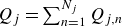 $Q_j=\sum _{n=1}^{N_j}Q_{j,n}$
. These parcels are ordered in the same manner as the local
$Q_j=\sum _{n=1}^{N_j}Q_{j,n}$
. These parcels are ordered in the same manner as the local $\psi _{1}$
streamfunction, which is ordered such that for outlet (inlet) faces, it is increasing in a clockwise (counter-clockwise) around a 1-D intersection line. Mapping of
$\psi _{1}$
streamfunction, which is ordered such that for outlet (inlet) faces, it is increasing in a clockwise (counter-clockwise) around a 1-D intersection line. Mapping of $\psi _{1,j}$
to
$\psi _{1,j}$
to $\psi _{1,k}$
via the fracture mixing map
$\psi _{1,k}$
via the fracture mixing map ${\mathcal{M}_F}$
is then given in terms of the flow rates leaving
${\mathcal{M}_F}$
is then given in terms of the flow rates leaving $f_j$
and entering
$f_j$
and entering $f_k$
as
$f_k$
as
 \begin{equation} Q_j\psi _{1,j}=\sum _{n=1}^{n^o-1}Q_{j,n}+\psi _{1}^\star Q_{j,n^o}, \end{equation}
where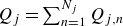 $Q_j=\sum _{n=1}^{N_j}Q_{j,n}$
is the total flow rate flowing through outlet face
$Q_j=\sum _{n=1}^{N_j}Q_{j,n}$
is the total flow rate flowing through outlet face $f_j$
, and the critical streamnumber
$f_j$
, and the critical streamnumber $\psi _1^\star$
quantifies the proportion of the flux
$\psi _1^\star$
quantifies the proportion of the flux $Q_{j,n^o}$
that corresponds to the streamline quantified by
$Q_{j,n^o}$
that corresponds to the streamline quantified by $\psi _{1,j}$
. In (B18),
$\psi _{1,j}$
. In (B18), $n_o$
is the number of the streamline parcel that contains the streamline with local streamfunction
$n_o$
is the number of the streamline parcel that contains the streamline with local streamfunction $\psi _{1,j}$
, which satisfies
$\psi _{1,j}$
, which satisfies
 \begin{equation} \sum _{n=1}^{n^o-1}Q_{j,n}\lt Q_j\psi _{1,j}\leqslant \sum _{n=1}^{n^o}Q_{j,n}. \end{equation}
From (B18) and (B19), both $n^o$
and
$n^o$
and $\psi _1$
can be computed directly from the flow rates
$\psi _1$
can be computed directly from the flow rates $Q_{j,n}$
leaving
$Q_{j,n}$
leaving $f_j$
and the streamfunction
$f_j$
and the streamfunction $\psi _{1,j}$
. Similarly,
$\psi _{1,j}$
. Similarly, $\psi _{1,k}$
and the parcel
$\psi _{1,k}$
and the parcel $n_i$
that contains the streamline entering
$n_i$
that contains the streamline entering $f_k$
are computed as
$f_k$
are computed as
 \begin{equation} Q_k\psi _{1,k}=\sum _{n=1}^{n^i-1}Q_{k,n}+\psi _{1}^\star Q_{k,n^i}, \end{equation}
where $n_i$
satisfies
$n_i$
satisfies
 \begin{equation} \sum _{n=1}^{n^i-1}Q_{k,n}\lt Q_k\psi _{1,k}\leqslant \sum _{n=1}^{n^i}Q_{k,n}. \end{equation}
Hence, (B18)–(B21) define the fracture mixing map ${\mathcal{M}_F}$
and facilitate updating of
${\mathcal{M}_F}$
and facilitate updating of $\psi _{1,j}\mapsto \psi _{1,k}$
as well as the edge mapping
$\psi _{1,j}\mapsto \psi _{1,k}$
as well as the edge mapping $j\mapsto k$
. Together, the mixing maps
$j\mapsto k$
. Together, the mixing maps ${\mathcal{M}_I}$
,
${\mathcal{M}_I}$
, ${\mathcal{M}_F}$
determine the local stream numbers (
${\mathcal{M}_F}$
determine the local stream numbers ( $\psi _{1,n}$
,
$\psi _{1,n}$
, $\psi _{2,n}$
) and the faces
$\psi _{2,n}$
) and the faces $f_n$
that streamlines visit as they propagate through the network.
$f_n$
that streamlines visit as they propagate through the network.
The mixing graph ${\mathcal{G}_M}$
(which quantifies the fracture network topology and fluxes as a WADG), along with the ordering and orientation of fluid parcels from face to face (edge to edge) throughout the fracture network (graph) is sufficient to fully characterise the PWI intersection maps
${\mathcal{G}_M}$
(which quantifies the fracture network topology and fluxes as a WADG), along with the ordering and orientation of fluid parcels from face to face (edge to edge) throughout the fracture network (graph) is sufficient to fully characterise the PWI intersection maps ${\mathcal{M}_I}$
and the fracture maps
${\mathcal{M}_I}$
and the fracture maps ${\mathcal{M}_F}$
. For the PWS intersection maps
${\mathcal{M}_F}$
. For the PWS intersection maps ${\mathcal{M}_I}$
, the monotone maps
${\mathcal{M}_I}$
, the monotone maps $\varPsi _{1,n}(x_1)$
or
$\varPsi _{1,n}(x_1)$
or $X_{1,n}(\psi _1)$
must also be determined at each face throughout the network. As this can be achieved efficiently via spline functions, both the PWI and PWS models generate parsimonious representations of the Lagrangian kinematics and thus advective mixing within fracture networks.
$X_{1,n}(\psi _1)$
must also be determined at each face throughout the network. As this can be achieved efficiently via spline functions, both the PWI and PWS models generate parsimonious representations of the Lagrangian kinematics and thus advective mixing within fracture networks.
Appendix C. Mixing measures
The evolution of the concentration field within the fracture network can be characterised in terms of the local concentration mean $\bar {c}_n$
and variance
$\bar {c}_n$
and variance $\sigma ^2_n$
at each face
$\sigma ^2_n$
at each face $f_n$
, which are defined as
$f_n$
, which are defined as
 \begin{align} \bar {c}_n\equiv \int _0^1\int _0^1 c_n(\psi _1,\psi _2)\,\text{d}\psi _1\,\text{d}\psi _2&& \sigma _{c_n}^2\equiv \int _0^1\int _0^1 [c_n(\psi _1,\psi _2)-\bar {c}_n]^2 \,\text{d}\psi _1\,\text{d}\psi _2. \end{align}
Although these measures can vary at each face $f_n$
within the DFN, the global inlet concentration mean and variance,
$f_n$
within the DFN, the global inlet concentration mean and variance,
 \begin{align} \bar {c}_{0}\equiv \frac {1}{Q}\sum _{n=1}^{N_{I_i}}Q_n \bar {c}_n, && \sigma _{0}^2\equiv \frac {1}{Q}\sum _{n=1}^{N_{I_i}}Q_n\left (\sigma _{c_n}^2+\bar {c}_0^2-\bar {c}_n^2\right ), \end{align}
are preserved throughout the fracture network in the sense that the global outlet mean and variance are equivalent
 \begin{align} \bar {c}_{\textit{out}}\equiv \frac {1}{Q}\sum _{n=N_I-N_{I_o}}^{N_I}Q_n \bar {c}_n = \bar {c}_0, && \sigma _{\textit{out}}^2\equiv \frac {1}{Q}\sum _{n=N_I-N_{I_o}}^{N_I}Q_n\left (\sigma _{c_n}^2+\bar {c}_{\textit{out}}^2-\bar {c}_n^2\right )=\sigma _0^2, \end{align}
due to the non-dissipative nature of purely advective mixing. A different mixing measure is the mix-norm metric (Mathew et al. Reference Mathew, Mezić and Petzold2005), a multi-scale mixing measure which robustly measures the degree of mixing by integrating over a scale-dependent concentration variance. The mix-norm is maximal if the concentration field is separated at the largest possible scale (such as the concentration distributions shown in figures 2
a and 2
b), and vanishes if and only if the scalar field is perfectly homogenised at the smallest scale (Thiffeault Reference Thiffeault2012). The mix-norm can be computed from the global outlet concentration field $ c_{\textit{out}}(\hat \psi _{1},\hat \psi _{2})$
in terms of the rescaled (dimensional) global streamfunctions
$ c_{\textit{out}}(\hat \psi _{1},\hat \psi _{2})$
in terms of the rescaled (dimensional) global streamfunctions $\hat \psi _1^\prime \equiv L\, \hat \psi _1\in [0,L]$
,
$\hat \psi _1^\prime \equiv L\, \hat \psi _1\in [0,L]$
, $\hat \psi _2^\prime \equiv \ell \, \hat \psi _2\in [0,\ell ]$
as follows. First, we define the average of
$\hat \psi _2^\prime \equiv \ell \, \hat \psi _2\in [0,\ell ]$
as follows. First, we define the average of $c_{\textit{out}}-\bar {c}_0$
over a square of dimension
$c_{\textit{out}}-\bar {c}_0$
over a square of dimension $s$
centred over
$s$
centred over $\hat \psi _1$
,
$\hat \psi _1$
, $\hat \psi _2$
as
$\hat \psi _2$
as
 \begin{equation} { d}\big(s, \hat \psi _1^\prime ,\hat \psi _2^\prime \big) \equiv \frac {\ell \,L}{s^2} \int _{\max \big(\hat \psi _1^\prime - s/2,0\big)}^{\min \big(\hat \psi _1^\prime + s/2,L\big)} \int _{\max \big(\hat \psi _2^\prime - s/2,0\big)}^{\min \big(\hat \psi _2^\prime + s/2,\ell \big)} c_{\textit{out}}(\xi _1/L, \xi _2/\ell )-\bar {c}_0 \, \text{d}\xi _2 \, \text{d}\xi _1. \end{equation}
Note that for $s\gt \ell$
, all variance in
$s\gt \ell$
, all variance in $c_{\textit{out}}$
with respect to
$c_{\textit{out}}$
with respect to $\hat \psi _2^\prime$
is integrated out in (C4), hence,
$\hat \psi _2^\prime$
is integrated out in (C4), hence, $d^2$
is not a function of
$d^2$
is not a function of $\hat \psi _2^\prime$
for
$\hat \psi _2^\prime$
for $s\gt \ell$
. The square of this fluctuation is then integrated over
$s\gt \ell$
. The square of this fluctuation is then integrated over $\hat \psi _1\prime$
,
$\hat \psi _1\prime$
, $\hat \psi _2\prime$
to give the scale-dependent variance
$\hat \psi _2\prime$
to give the scale-dependent variance $\phi ^2(s)$
with
$\phi ^2(s)$
with $s\in [0,L]$
as
$s\in [0,L]$
as
 \begin{equation} \phi ^2(s) \equiv \frac {1}{\ell \, L}\int _0^L \int _0^\ell d^2\big(s,\hat \psi _1^\prime ,\hat \psi _2^\prime \big) \, \text{d}\hat \psi _1^\prime \, \text{d}\hat \psi _2^\prime , \end{equation}
such that for $s\gt \ell$
,
$s\gt \ell$
, $\phi ^2(s)$
only depends on variations in the
$\phi ^2(s)$
only depends on variations in the $\hat \psi _1$
direction. Integrating this scale-dependent variance over
$\hat \psi _1$
direction. Integrating this scale-dependent variance over $s$
yields the 2-D mix-norm
$s$
yields the 2-D mix-norm $\varPhi ^2_{2\textit{-D}}$
 \begin{equation} \begin{aligned} \varPhi ^2_{2\textit{-D}} \equiv \frac {1}{L}\int _0^L \phi ^2(c_{\textit{out}}, s) \, \text{d}s =&\frac {1}{L}\int _0^\ell \phi ^2(s) \, \text{d}s +\frac {1}{L}\int _\ell ^L \phi ^2(s) \, \text{d}s ,\\ =&\varPhi ^2_{2\textit{-D},\ell }+\varPhi ^2_{2\textit{-D},L} \end{aligned} \end{equation}
which quantifies the degree of mixing from the smallest scale $s=0$
to the largest scale
$s=0$
to the largest scale $s=L$
. As shown in (C6), the mix-norm can be separated into the (
$s=L$
. As shown in (C6), the mix-norm can be separated into the ( $\hat \psi _1$
,
$\hat \psi _1$
, $\hat \psi _2$
)-dependent microscopic mix-norm
$\hat \psi _2$
)-dependent microscopic mix-norm $\varPhi ^2_{2\textit{-D},\ell }$
, which quantifies mixing over scales
$\varPhi ^2_{2\textit{-D},\ell }$
, which quantifies mixing over scales $s\in [0,\ell ]$
, and the
$s\in [0,\ell ]$
, and the $\hat \psi _1$
-dependent macroscopic mix-norm
$\hat \psi _1$
-dependent macroscopic mix-norm $\varPhi ^2_{2\textit{-D},L}$
, which quantifies mixing over scales
$\varPhi ^2_{2\textit{-D},L}$
, which quantifies mixing over scales $s\in [\ell ,L]$
. As
$s\in [\ell ,L]$
. As $\ell \ll L$
, then
$\ell \ll L$
, then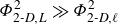 $\varPhi ^2_{2\textit{-D},L}\gg \varPhi ^2_{2\textit{-D},\ell }$
; hence, the mix-norm is accurately approximated by the macroscopic mix-norm as
$\varPhi ^2_{2\textit{-D},L}\gg \varPhi ^2_{2\textit{-D},\ell }$
; hence, the mix-norm is accurately approximated by the macroscopic mix-norm as
 \begin{equation} \varPhi ^2_{2\textit{D}}(c_{\textit{out}})=\varPhi ^2_{2\textit{D},L}(c_{\textit{out}})+\mathcal{O}(\ell /L). \end{equation}
As the macroscopic mix-norm only depends upon $\hat \psi _1$
, (C7) suggests that mixing in fracture networks can be accurately quantified as a 1-D process. We note however that both streamfunctions are critical to modelling processes such as intersection mixing at arbitrary Péclet number.
$\hat \psi _1$
, (C7) suggests that mixing in fracture networks can be accurately quantified as a 1-D process. We note however that both streamfunctions are critical to modelling processes such as intersection mixing at arbitrary Péclet number.
Examples of 1-D mixing plots for fracture networks that exhibit (a) no mixing ( $\hat \psi _1^{\textit{out}}=\hat \psi _1$
), (b) fracture mixing only (figure 2
a), (c) intersection mixing only (figure 2
c) , and (d) combined intersection and fracture mixing (figure 1
b). The top horizontal strip on each plot shows the inlet 1-D concentration distribution
$\hat \psi _1^{\textit{out}}=\hat \psi _1$
), (b) fracture mixing only (figure 2
a), (c) intersection mixing only (figure 2
c) , and (d) combined intersection and fracture mixing (figure 1
b). The top horizontal strip on each plot shows the inlet 1-D concentration distribution $c_0(\hat \psi _1)$
and the right vertical strip shows the outlet 1-D concentration distribution
$c_0(\hat \psi _1)$
and the right vertical strip shows the outlet 1-D concentration distribution $c_{\textit{out}}(\hat \psi _1)$
that correspond to the 2-D concentration fields shown in figures 2(b) and 2(d) and the associated faces are denoted
$c_{\textit{out}}(\hat \psi _1)$
that correspond to the 2-D concentration fields shown in figures 2(b) and 2(d) and the associated faces are denoted $f_n$
. Each plot shows the global streamfunction mapping
$f_n$
. Each plot shows the global streamfunction mapping $\hat \psi _1\mapsto \hat \psi _1^{\textit{out}}$
(indicated by black arrows) that also maps
$\hat \psi _1\mapsto \hat \psi _1^{\textit{out}}$
(indicated by black arrows) that also maps $c_0\mapsto c_{\textit{out}}$
, and each point (which is coloured with respect to its inlet concentration value
$c_0\mapsto c_{\textit{out}}$
, and each point (which is coloured with respect to its inlet concentration value $c_0$
) in the
$c_0$
) in the $\hat \psi _1-\hat \psi _1^{\textit{out}}$
plane corresponds to a given streamline; hence, continuous sets of streamlines form lines in the 1-D mixing plot. Fracture mixing in panel (b) acts to macroscopically cut and shuffle continuous segments of lines along
$\hat \psi _1-\hat \psi _1^{\textit{out}}$
plane corresponds to a given streamline; hence, continuous sets of streamlines form lines in the 1-D mixing plot. Fracture mixing in panel (b) acts to macroscopically cut and shuffle continuous segments of lines along $\hat \psi _1^{\textit{out}}$
, whereas intersection mixing in panel (c) acts to microscopically cut and shuffles individual streamlines with respect to
$\hat \psi _1^{\textit{out}}$
, whereas intersection mixing in panel (c) acts to microscopically cut and shuffles individual streamlines with respect to $\hat \psi _2^{\textit{out}}$
(not resolved), leading to ‘overlap’ (grey region) of streamlines with the same
$\hat \psi _2^{\textit{out}}$
(not resolved), leading to ‘overlap’ (grey region) of streamlines with the same $\psi _1^{\textit{out}}$
but different
$\psi _1^{\textit{out}}$
but different $c_0$
values that thus generate
$c_0$
values that thus generate $1\lt c_{\textit{out}}(\hat \psi _1)\lt 0$
. Panel (d) shows the one-dimensional mixing plot for the fracture network shown in figure 1(b) and its corresponding mixing graph
$1\lt c_{\textit{out}}(\hat \psi _1)\lt 0$
. Panel (d) shows the one-dimensional mixing plot for the fracture network shown in figure 1(b) and its corresponding mixing graph ${\mathcal{G}_M}$
representation in figure 10. Horizontal and vertical bars respectively indicate inlet
${\mathcal{G}_M}$
representation in figure 10. Horizontal and vertical bars respectively indicate inlet $c_0(\hat \psi _1)$
and outlet
$c_0(\hat \psi _1)$
and outlet $c_{\textit{out}}(\hat \psi _1)$
concentration distributions,
$c_{\textit{out}}(\hat \psi _1)$
concentration distributions, $f_n$
indicates inlet and outlet faces, coloured lines in the
$f_n$
indicates inlet and outlet faces, coloured lines in the $\hat \psi _1-\hat \psi _1^{\textit{out}}$
plane indicate streamlines that are cut and shuffled via both fracture and intersection mixing, and grey bars indicate ‘overlap’ regions where intersection mixing occurs (and hence dilution of
$\hat \psi _1-\hat \psi _1^{\textit{out}}$
plane indicate streamlines that are cut and shuffled via both fracture and intersection mixing, and grey bars indicate ‘overlap’ regions where intersection mixing occurs (and hence dilution of $c_{\textit{out}}(\hat \psi _1)$
).
$c_{\textit{out}}(\hat \psi _1)$
).

Appendix D. One-dimensional mixing plots
Associated with the 1-D mixing representation (3.22) are the 1-D mixing plots shown in figure 18 which provide a simplified representation of mixing over the entire fracture network. These plots show how the global streamfunction $\hat \psi _1$
over the network inlets is mapped to the outlet global streamfunction
$\hat \psi _1$
over the network inlets is mapped to the outlet global streamfunction $\hat \psi _1^{\textit{out}}$
over the outlets, and so represent cutting and shuffling of streamlines with respect to the
$\hat \psi _1^{\textit{out}}$
over the outlets, and so represent cutting and shuffling of streamlines with respect to the $\hat {\psi }_1$
coordinate. These plots also show how the step-wise inlet concentration field
$\hat {\psi }_1$
coordinate. These plots also show how the step-wise inlet concentration field $c_0(\hat \psi _1)=H(1/2-\hat \psi _1)$
(where
$c_0(\hat \psi _1)=H(1/2-\hat \psi _1)$
(where $H$
is the Heaviside step function) is mapped to the outlet concentration field
$H$
is the Heaviside step function) is mapped to the outlet concentration field $c_{\textit{out}}(\hat \psi _1)$
, where the colour bars in figure 18 may be considered as 1-D analogues (
$c_{\textit{out}}(\hat \psi _1)$
, where the colour bars in figure 18 may be considered as 1-D analogues ( $\hat {\psi _1}$
only) of the 2-D inlet and outlet concentration fields shown in figure 10.
$\hat {\psi _1}$
only) of the 2-D inlet and outlet concentration fields shown in figure 10.
To clearly explain these plots, we first consider the 1-D mixing plot shown in figure 18(a) for the trivial case of a fracture network with no mixing ( $\hat \psi _1^{\textit{out}}=\hat \psi _1$
). For this plot, each streamline advected through the network arises as a discrete point (with colour corresponding to
$\hat \psi _1^{\textit{out}}=\hat \psi _1$
). For this plot, each streamline advected through the network arises as a discrete point (with colour corresponding to $c_0(\hat {\psi }_1)$
) in the
$c_0(\hat {\psi }_1)$
) in the $\hat \psi _1{-}\hat \psi _1^{\textit{out}}$
plane. Hence, these points form a 45
$\hat \psi _1{-}\hat \psi _1^{\textit{out}}$
plane. Hence, these points form a 45 $^\circ$
line which is red from
$^\circ$
line which is red from $(0,0)$
to
$(0,0)$
to $(1/2,1/2)$
and blue from
$(1/2,1/2)$
and blue from $(1/2,1/2)$
to
$(1/2,1/2)$
to $(1,1)$
, and the inlet and outlet concentration distributions are identical as
$(1,1)$
, and the inlet and outlet concentration distributions are identical as $c(\hat \psi _1)=c(\hat \psi _1^{\textit{out}})=c_{\textit{out}}(\hat \psi _1)$
.
$c(\hat \psi _1)=c(\hat \psi _1^{\textit{out}})=c_{\textit{out}}(\hat \psi _1)$
.
Figure 18(b) shows the 1-D mixing plot generated by the network shown in figure 2(a) that exhibits fracture mixing only. For this network, streamline routing within fractures generates CS of streamlines with respect to the $\psi _1$
coordinate, leading to the 2-D and 1-D concentration distributions shown respectively in figures 2(b) and 18(b). The latter figure highlights how fracture mixing acts to cut and shuffle sets of points along the vertical
$\psi _1$
coordinate, leading to the 2-D and 1-D concentration distributions shown respectively in figures 2(b) and 18(b). The latter figure highlights how fracture mixing acts to cut and shuffle sets of points along the vertical $\hat \psi _1^{\textit{out}}$
axis, which repositions (and in some cases, reflects) segments of the 45
$\hat \psi _1^{\textit{out}}$
axis, which repositions (and in some cases, reflects) segments of the 45 $^\circ$
line shown in figure 18(b). This results in large-scale fracture mixing of the 1-D concentration distribution
$^\circ$
line shown in figure 18(b). This results in large-scale fracture mixing of the 1-D concentration distribution $c(\hat \psi _1^{\textit{out}})$
shown in figure 18(b), which is equivalent to the 2-D concentration distribution
$c(\hat \psi _1^{\textit{out}})$
shown in figure 18(b), which is equivalent to the 2-D concentration distribution $c(\psi _{1,n},\psi _{2,n})$
shown in figure 2(b). Note that although values of the 1-D concentration field are unchanged
$c(\psi _{1,n},\psi _{2,n})$
shown in figure 2(b). Note that although values of the 1-D concentration field are unchanged $c_{\textit{out}}(\hat \psi _1)\in \{0,1\}$
, the 1-D scale-dependent variance
$c_{\textit{out}}(\hat \psi _1)\in \{0,1\}$
, the 1-D scale-dependent variance $\phi ^2_{1\textit{-D}}(s)$
and mix-norm
$\phi ^2_{1\textit{-D}}(s)$
and mix-norm $\varPhi ^2_{1\textit{-D}}$
decrease due to large-scale cutting and shuffling of the concentration field
$\varPhi ^2_{1\textit{-D}}$
decrease due to large-scale cutting and shuffling of the concentration field $c_{\textit{out}}(\hat \psi _1)$
. Repeat random fracture mixing processes would cut and shuffle this 1-D concentration distribution into smaller contiguous segments, driving
$c_{\textit{out}}(\hat \psi _1)$
. Repeat random fracture mixing processes would cut and shuffle this 1-D concentration distribution into smaller contiguous segments, driving $\varPhi ^2_{1\textit{-D}}\rightarrow 0$
, but the concentration values would still be limited to
$\varPhi ^2_{1\textit{-D}}\rightarrow 0$
, but the concentration values would still be limited to $c_{\textit{out}}(\hat \psi _1)\in \{0,1\}$
.
$c_{\textit{out}}(\hat \psi _1)\in \{0,1\}$
.
Figure 18(c) shows the 1-D mixing plot generated by the network shown in figure 2(c) that exhibits intersection mixing only. For this network, streamline routing within intersections generates CS actions with respect to the $\psi _2$
coordinate, leading to the 2-D and 1-D concentration distributions shown respectively in figures 2(d) and 18(c). For intersection mixing, the points (streamlines) that comprise the 45
$\psi _2$
coordinate, leading to the 2-D and 1-D concentration distributions shown respectively in figures 2(d) and 18(c). For intersection mixing, the points (streamlines) that comprise the 45 $^\circ$
line in figure 18(a) are cut and shuffled according to their
$^\circ$
line in figure 18(a) are cut and shuffled according to their $\hat \psi _2$
coordinate. In figure 18(c), this manifests as half the points along this line being reflected along the
$\hat \psi _2$
coordinate. In figure 18(c), this manifests as half the points along this line being reflected along the $\hat \psi _1^{\textit{out}}=1/2$
line, leading to multiple streamlines (points) with the same
$\hat \psi _1^{\textit{out}}=1/2$
line, leading to multiple streamlines (points) with the same $\hat \psi _1^{\textit{out}}$
streamfunction but different
$\hat \psi _1^{\textit{out}}$
streamfunction but different $\hat \psi _1$
(and thus
$\hat \psi _1$
(and thus $c_0$
) values. This ‘overlap’ with respect to
$c_0$
) values. This ‘overlap’ with respect to $\hat \psi _1^{\textit{out}}$
, which does not occur under fracture mixing (figure 18
b), is a clear signature of intersection mixing. Here, the
$\hat \psi _1^{\textit{out}}$
, which does not occur under fracture mixing (figure 18
b), is a clear signature of intersection mixing. Here, the $c=0$
and
$c=0$
and $c=1$
streamlines have the same
$c=1$
streamlines have the same $\hat \psi _1^{\textit{out}}$
value, and so these concentrations are averaged according to (3.22), leading to dilution of the outlet 1-D concentration
$\hat \psi _1^{\textit{out}}$
value, and so these concentrations are averaged according to (3.22), leading to dilution of the outlet 1-D concentration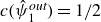 $c(\hat \psi _1^{\textit{out}})=1/2$
distribution, which is homogeneous according to the mixing measures
$c(\hat \psi _1^{\textit{out}})=1/2$
distribution, which is homogeneous according to the mixing measures $\phi ^2_{1\textit{-D}}(s)=\varPhi ^2_{1\textit{-D}}=0$
. Note that the fully resolved outlet 2-D concentration distribution (figure 10
d) has concentration values limited to
$\phi ^2_{1\textit{-D}}(s)=\varPhi ^2_{1\textit{-D}}=0$
. Note that the fully resolved outlet 2-D concentration distribution (figure 10
d) has concentration values limited to $c=\{0,1\}$
, and so its variance is unchanged. This discrepancy is solely due to the microscopic nature of intersection mixing – as it mixes at length scales
$c=\{0,1\}$
, and so its variance is unchanged. This discrepancy is solely due to the microscopic nature of intersection mixing – as it mixes at length scales $s\lesssim \ell$
, it is represented as fully mixed under the macroscopic 1-D representation
$s\lesssim \ell$
, it is represented as fully mixed under the macroscopic 1-D representation $s\gt \ell$
, but unmixed under the 2-D representation. As per (3.23), under such intersection mixing,
$s\gt \ell$
, but unmixed under the 2-D representation. As per (3.23), under such intersection mixing, $\phi ^2_{1\textit{-D}}(s)=0$
and
$\phi ^2_{1\textit{-D}}(s)=0$
and $\phi ^2_{2\textit{-D}}(s)\neq 0$
for
$\phi ^2_{2\textit{-D}}(s)\neq 0$
for $s\lt \ell$
, but
$s\lt \ell$
, but $\phi ^2_{1\textit{-D}}=\phi ^2_{2\textit{-D}}=0$
for
$\phi ^2_{1\textit{-D}}=\phi ^2_{2\textit{-D}}=0$
for $\ell \lt s\lt L$
; hence,
$\ell \lt s\lt L$
; hence, $\varPhi ^2_{1\textit{-D}}\approx \varPhi ^2_{2\textit{-D}}$
.
$\varPhi ^2_{1\textit{-D}}\approx \varPhi ^2_{2\textit{-D}}$
.
Figure 18(d) shows the 1-D mixing plot for the fracture network shown in figure 1(b) and the corresponding 2-D concentration fields shown in figure 10. The outlet faces in figure 10 show clear evidence of both fracture mixing (CS with respect to $\psi _{1,n}$
) and intersection mixing (CS with respect to
$\psi _{1,n}$
) and intersection mixing (CS with respect to $\psi _{2,n}$
). Similarly, the 1-D outlet concentration field
$\psi _{2,n}$
). Similarly, the 1-D outlet concentration field $c_{\textit{out}}(\hat \psi _1)$
in figure 18(d) shows clear evidence of CS along
$c_{\textit{out}}(\hat \psi _1)$
in figure 18(d) shows clear evidence of CS along $\hat \psi _1^{\textit{out}}$
and dilution due to CS along
$\hat \psi _1^{\textit{out}}$
and dilution due to CS along $\hat \psi _2^{\textit{out}}$
. Similarly, the mapping of lines in the
$\hat \psi _2^{\textit{out}}$
. Similarly, the mapping of lines in the $(\hat \psi _1, \hat \psi _1^{\textit{out}})$
plane show signatures of both fracture mixing from figure 18(b) and intersection mixing from figure 18(c), the latter of which leads to the overlap regions shown in figure 18(d) and dilution of
$(\hat \psi _1, \hat \psi _1^{\textit{out}})$
plane show signatures of both fracture mixing from figure 18(b) and intersection mixing from figure 18(c), the latter of which leads to the overlap regions shown in figure 18(d) and dilution of $c_{\textit{out}}(\hat \psi _1)$
.
$c_{\textit{out}}(\hat \psi _1)$
.


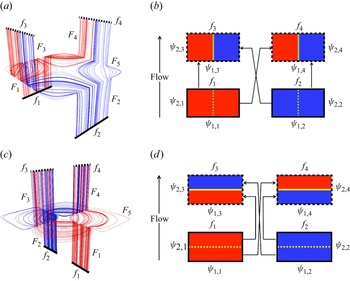


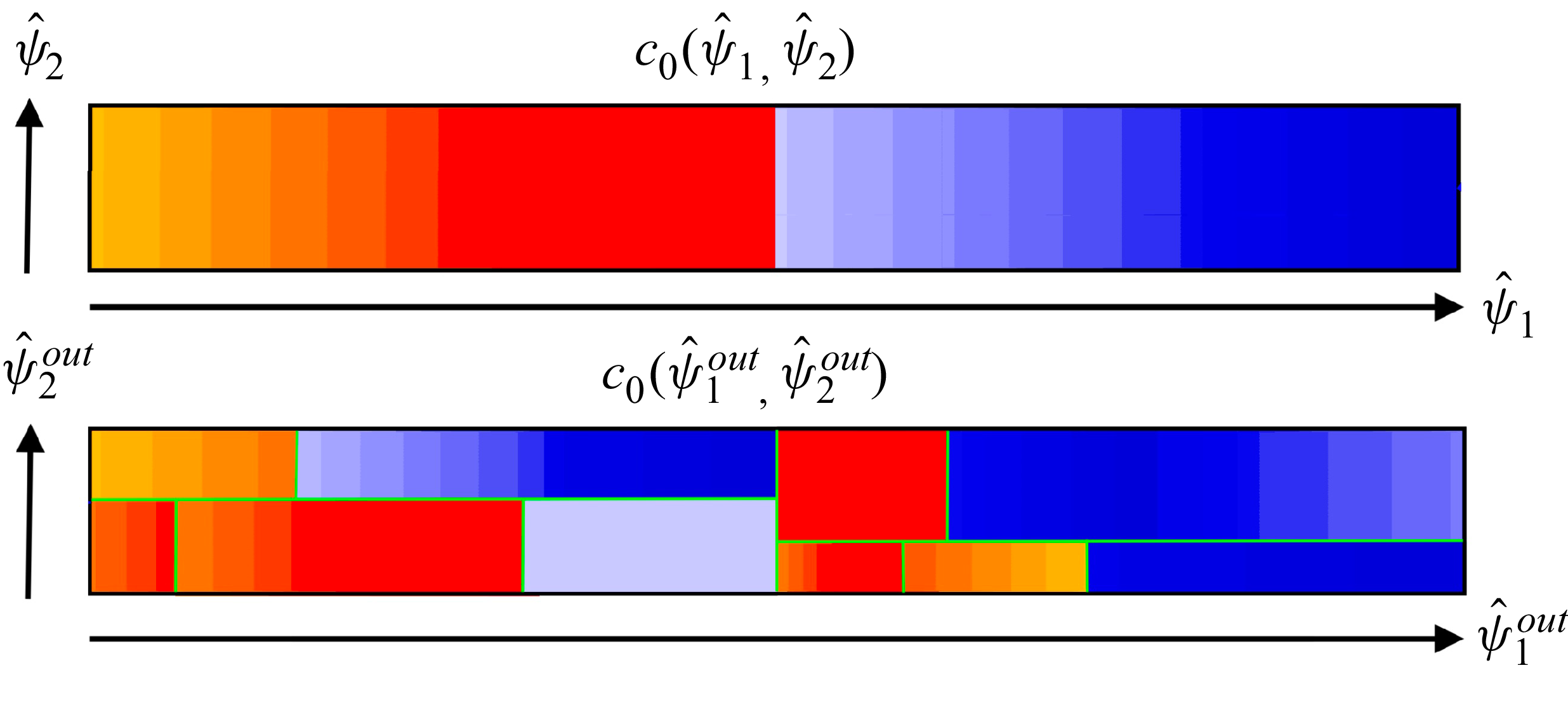


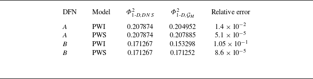


 Open access

