


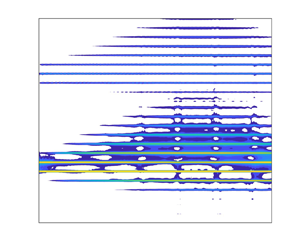



1. Introduction
Numerical solutions for free-surface flows can be obtained by solving the Navier–Stokes (N–S) equations with necessary boundary conditions. The free-surface location is part of the solution and the free-surface boundary conditions are nonlinear. When viscous/turbulent effects are negligible, the N–S equations reduce to Euler's equations. The direct numerical solutions of N–S and Euler's equations are computationally expensive for three-dimensional (3-D) problems, especially for large-scale problems, since the solution solver for the pressure Poisson equation (PPE) requires a significant amount of computing time. Furthermore, tracking the location of the free surface is also challenging. An attractive alternative is the so-called depth-integrated models, in which the model equations are solved only in horizontal dimensions after certain approximations are invoked for the vertical profiles of the velocity and pressure fields. Theoretically speaking, with proper descriptions of lateral boundary conditions and initial conditions, appropriate numerical algorithms could be selected to solve these two-dimensional horizontal (2-DH) model equations for transient free-surface flows, including water wave propagation and scattering problems and transient/steady hydraulic flow problems. Based on the background and procedures for deriving existing 2-DH models, they can be divided into two general categories: Boussinesq-type models and Green–Naghdi-type models. A brief review of each category is provided as follows.
Denoting  $H$ as the characteristic wave height, $k$ as the characteristic wavenumber and $h$ as the water depth, Boussinesq-type models adopt the Boussinesq approximation, where the nonlinearity, $\epsilon = H/h$, and frequency dispersion, $\mu ^2 =(kh)^2$, are equally small and require flows to be irrotational or weakly rotational. The traditional Boussinesq models are of $O(\mu ^2)$ (Peregrine Reference Peregrine1967). Over the last 40 years, great efforts have been made to extend the applicable range of the traditional Boussinesq equations from relatively shallow to deeper water and from weak to full nonlinearity (e.g. Madsen & Sørensen Reference Madsen and Sørensen1992; Nwogu Reference Nwogu1993; Liu Reference Liu1995; Wei et al. Reference Wei, Kirby, Grilli and Subramanya1995; Gobbi, Kirby & Wei Reference Gobbi, Kirby and Wei2000; Madsen & Agnon Reference Madsen and Agnon2003; Lynett & Liu Reference Lynett and Liu2004; Liu, Fang & Cheng Reference Liu, Fang and Cheng2018). Generally speaking, it is relatively straightforward to include the full nonlinearity. Wei et al. (Reference Wei, Kirby, Grilli and Subramanya1995) and Liu (Reference Liu1995) presented such models by specifying $\epsilon = O(1)$ and expanding the governing equations and boundary conditions only in terms of $\mu ^2$. These fully nonlinear models no longer satisfy the Boussinesq approximation. However, they have been called the Boussinesq-type models in the literature. It is more challenging to expand the model capability into deep-water depth regimes. Gobbi et al. (Reference Gobbi, Kirby and Wei2000) introduced the standard higher-order ( $\mu ^4$) extension of the traditional $\mu ^2$ Boussinesq model (Nwogu Reference Nwogu1993). Although the resulting model can indeed be applied to a deeper-water regime, the model equations contain fifth-order derivatives, requiring more boundary conditions and greater computing effort.
To avoid these issues, Lynett & Liu (Reference Lynett and Liu2004) introduced the multi-layer model concept. In their model, the wave motions in each layer satisfy the Boussinesq approximation, and the vertical profile of the horizontal velocity in each layer is approximated by quadratic polynomials being matched at the layer interface with the horizontal velocity in the adjacent layer. The resulting model only consists of spatial derivatives up to three. An alternative approach was first proposed by Agnon, Madsen & Schäffer (Reference Agnon, Madsen and Schäffer1999) and further developed by Madsen, Bingham & Liu (Reference Madsen, Bingham and Liu2002), whose approach was formulated based on the exact boundary condition and the approximated solution of the Laplace equation for irrotational flow. The vertical velocity component is retained in the formulation, and the resulting model consists of six coupled equations solving for free-surface elevations, horizontal gradient of the velocity potential at the surface, horizontal and vertical velocity components at the still water level and computational horizontal and vertical velocity components at an arbitrary level.
In general, Boussinesq-type models are useful tools for simulating wave transformations from deep water to shallow water, while maintaining a good balance between efficiency and accuracy. However, most Boussinesq-type models are only applicable up to the deep-water limit, which is restricted by the weakly dispersive assumption in the Boussinesq approximation. The basic assumption of weak rotationality further restricts models’ applications to wave–current interaction problems; only depth-uniform or very weakly sheared current can be considered in Boussinesq-type models. A concise literature review of these depth-integrated models can be found in Kirby (Reference Kirby2016).
Green–Naghdi-type models approximate the vertical profile of the velocity components, both horizontal and vertical, in a polynomial form in terms of the vertical coordinate. Following Kantorovich & Krylov (Reference Kantorovich and Krylov1958), the resulting momentum equations are satisfied in a weighted-averaged sense (Shields & Webster Reference Shields and Webster1988). If the vertical profile of the horizontal velocity is assumed to be depth-uniform, the simplest Green–Naghdi equations (Green, Laws & Naghdi Reference Green, Laws and Naghdi1974; Green & Naghdi Reference Green and Naghdi1976) or Serre equations (Serre Reference Serre1953) are derived, which have been used for studying waves generated by a moving pressure disturbance (Ertekin, Webster & Wehausen Reference Ertekin, Webster and Wehausen1986). Employing higher-degree polynomials for the velocity profiles, Webster, Duan & Zhao (Reference Webster, Duan and Zhao2011) derived more complicated Green–Naghdi-type models with more unknowns but better accuracy, which have been applied to study several wave transformation and wave–current interaction problems (Zhao, Duan & Ertekin Reference Zhao, Duan and Ertekin2014; Zhao et al. Reference Zhao, Li, Duan, Ertekin and Hayatdavoodi2023). However, in these models the vertical momentum equation was not satisfied exactly and the analytical expression for the non-hydrostatic pressure field was not available. Using a combined approach from Boussinesq-type shallow-water wave scaling and the polynomial representation of the horizontal velocity in Green–Naghdi equations, Zhang et al. (Reference Zhang, Kennedy, Panda, Dawson and Westerink2013) derived the Boussinesq–Green–Naghdi rotational water wave theory. The free coefficients used in the polynomial approximation have been optimised to achieve the best model performance in terms of various linear and nonlinear wave properties.
Yang & Liu (Reference Yang and Liu2020) (referred to as YL20 herein) presented two sets of depth-integrated wave–current models. The major difference between models developed by YL20 and other existing models is that YL20 models are based on the depth-integrated continuity equation and momentum (Euler's) equations in terms of horizontal velocity components and free-surface elevation. As mentioned earlier, these equations are exact and the free surface and bottom boundary conditions are also satisfied. More importantly, the vertical velocity component and the pressure field can be expressed analytically in terms of the horizontal velocity and the free-surface elevation. Approximating the vertical profiles of the horizontal velocity components by polynomials, and using the Galerkin and subdomain methods, YL20 constructed GK and SK models, respectively. By a theoretical linear analysis, the SK models demonstrated better accuracy than GK models and Green–Naghdi-type models in terms of various wave properties. Both SK and GK models were also validated with several laboratory experiments. The SK models were also extended to simulate waves interacting with arbitrarily sheared currents (Yang & Liu Reference Yang and Liu2022), which cannot be handled by Boussinesq-type and Green–Naghdi-type models.
In both Green–Naghdi models and YL20 models, one polynomial of a certain degree is used to approximate the horizontal velocity profile in the entire water column, yielding models of different complexity and accuracy. In this study, we formalise the approximation of the horizontal velocity components in the water column by using the finite-element method (FEM; Zienkiewicz, Taylor & Zhu Reference Zienkiewicz, Taylor and Zhu2013), i.e. the water column is divided into several elements, and the horizontal velocity profile within each element is approximated by shape functions in terms of the vertical coordinate. Whereas the continuity of horizontal velocity is satisfied automatically, the vertical velocity and pressure fields at the finite-element nodes are enforced. The resulting residuals from the horizontal momentum equations are minimised via the method of weighted residuals (Zienkiewicz et al. Reference Zienkiewicz, Taylor and Zhu2013). A set of 2-DH equations for horizontal velocities at finite-element nodes is derived. In this paper, the linear shape functions are adopted, although the formulations can be readily extended to higher-order shape functions. A theoretical analysis shows that the new models significantly outperform Green–Naghdi models in terms of their applicability over the range of water depth to wavelength ratios, while maintaining the advantage of dealing with waves interacting with vertically sheared currents compared with Boussinesq-type models. The resulting 2-DH model equations can be solved by using appropriate numerical algorithms with prescribed lateral boundary conditions and initial conditions. In the present paper, models employing two linear elements and three linear elements are numerically implemented in the 1-D horizontal domain with a five-point central differencing combined with a fourth-order Runge–Kutta method for time integration. Various numerical validations are performed to study nonlinear Stokes wave and bichromatic wave group propagation in deep water, sideband instability in deep water, regular wave transformation over a submerged shoal and newly conducted experiments of focusing wave group interacting with linearly sheared currents in deep water, and very good agreement is obtained between the numerical results and laboratory experiments.
This paper is organised as follows. First, § 2 summarises the mathematical derivation of the depth-integrated model. A general derivation of models employing any number of linear elements is presented. An analytical analysis is carried out in § 3 to examine the Stokes-wave-type properties of the new models; their performance is compared with other depth-integrated models. The mathematical models are implemented numerically and validated by benchmark laboratory experiments in § 4. Numerical experiments of the wave shoaling process from deep water to shallow water are conducted and discussed in § 5. Finally, conclusions and drawn in § 6.
2. Derivation of the 2-DH model equations
2.1. Exact governing equations in three dimensions
Assuming viscous and turbulent effects are negligible, the present models are based on 3-D Euler's equations with boundary conditions for incompressible fluid bounded by a free surface and a stationary bottom. The sea bottom and the free surface are prescribed by  $z^*=-h(x^*,y^*)$ and $z^*=\eta (x^*,y^*,t^*)$, respectively, where the $x^*$- and $y^*$-axes are located at the still water level and the $z^*$-axis points upwards. A $\sigma$-coordinate transformation is introduced in this derivation to map the water column from $[-h, \eta ]$ in the Cartesian coordinate, to a fixed range of $[0, 1]$ in the $\sigma$-coordinate. This transformation is defined as follows:
 \begin{equation} t=t^*, \quad x_i={x_i}^*, \quad \sigma=\frac{z^*+h}{h+\eta}=\frac{z^*+h}{H},\end{equation}
where  $i =1,2$ and $(x_1 =x,\ x_2 =y)$. The independent variables in the $\sigma$-coordinate are $({x_i},\sigma,t)$ with $\sigma$ being a function of the free-surface elevation $\eta (x_i^*,t^*)$ and sea-bottom configuration $h(x_i^*)$. The total water depth has been denoted as $H=h+\eta$. Finally, the Euler's equations and boundary conditions in the $\sigma$-coordinate are
 \begin{gather} \frac{\partial u_i}{\partial x_i}+\frac{\partial u_i}{\partial \sigma}\sigma_{x_i}+\frac{\partial w}{\partial \sigma}\sigma_z=0, \end{gather}
 \begin{gather}\frac{\partial u_i}{\partial t}+\frac{\partial u_i}{\partial \sigma}\sigma_t+u_j\left(\frac{\partial u_i}{\partial x_j}+\frac{\partial u_i}{\partial \sigma}\sigma_{x_i}\right )+w\frac{\partial u_i}{\partial \sigma}\sigma_z ={-}\frac{1}{\rho}\left(\frac{\partial p}{\partial x_i}+\frac{\partial p}{\partial \sigma}\sigma_{x_i}\right) , \end{gather}
 \begin{gather}\frac{\partial w}{\partial t}+\frac{\partial w}{\partial \sigma}\sigma_t+u_j \left (\frac{\partial w}{\partial x_j}+\frac{\partial w}{\partial \sigma}\sigma_{x_i}\right )+w \frac{\partial w}{\partial \sigma}\sigma_z ={-}\frac{1}{\rho}\frac{\partial p}{\partial \sigma}\sigma_z-g, \end{gather}
 \begin{gather} p|_s=0, \quad \sigma=1, \end{gather}
 \begin{gather}\frac{\partial \eta}{\partial t}+u_i|_s\frac{\partial \eta}{\partial x_i}=w|_s, \quad \sigma=1, \end{gather}
 \begin{gather}u_i|_b\frac{\partial h}{\partial x_i}+w|_b=0, \quad \sigma=0, \end{gather}
where  $u_i\ (i=1,2)$ and $w$ are the horizontal and vertical velocity components, respectively, and $p$ is the pressure field. The subscript $s$ and $b$ denote the physical variables being evaluated at the free surface and bottom, respectively. Here, the density of water, $\rho$, and the gravitational acceleration, $g$, are constants. The Euler's equations consist of continuity equation (2.2) and horizontal and vertical momentum equations (2.3) and (2.4), respectively. On the free surface, the dynamic and kinematic boundary conditions are specified in (2.5) and (2.6), respectively. Along the solid bottom, (2.7) represents the no-flux condition. Lastly, $\sigma _{t}$, $\sigma _{x_i}$, and $\sigma _{z}$ denote the partial derivatives of $\sigma$ with respect to $t^*$, $x_i^*$ and $z^*$, respectively, which can be obtained by the chain rule as follows:
 \begin{equation} \sigma_{t}={-}\sigma\frac{1}{H}\frac{\partial H}{\partial t}, \quad \sigma_{x_i}=\frac{1}{H}\left(\frac{\partial h}{\partial x_i}-\sigma\frac{\partial H}{\partial x_i}\right), \quad \sigma_{z}=\frac{1}{H}. \end{equation}
To close the problem, appropriate lateral boundary conditions and initial conditions need to be prescribed.
It is well-known that the governing equations and boundary conditions shown in (2.2)–(2.7) can be combined into a set of governing equations for the horizontal velocity components, which depend on the vertical coordinate. The procedure is outlined as follows. By vertically integrating the continuity equation (2.2) from  $\sigma =0$ to 1 and applying the boundary conditions, (2.6) and (2.7), the well-known depth-integrated continuity equation can be obtained, i.e.
 \begin{equation} \frac{\partial H}{\partial t}+\frac{\partial}{\partial x_i}\left [\int_{0}^{1}(H u_i) \,\mathrm{d}\sigma \right ]=0.\end{equation}
Note that the above equation is exact and represents the mass conservation, integrated over the water column.
On the other hand, the vertical velocity can be derived by vertically integrating the continuity equation (2.2) from the bottom ( $\sigma =0$) to an arbitrary elevation in the water column and applying the kinematic boundary condition (2.7) at the bottom. Thus,
 \begin{equation} w={-}{u_i}|_b\frac{\partial h}{\partial x_i}-H\left [\int_0^\sigma \left ( \frac{\partial u_i}{\partial x_i}+\frac{\partial u_i}{\partial \sigma}\sigma_{x_i} \right )\, \mathrm{d}\sigma\right ].\end{equation}
Similarly, the expression for the pressure field is derived by vertically integrating the vertical momentum equation (2.4) from an arbitrary elevation to the free surface ( $\sigma =1$) and applying the dynamic boundary condition (2.5). Hence,
 \begin{equation} p=\rho H\left[ g (1-\sigma)+ \int_\sigma^{1} \left(\frac{\partial w}{\partial t}+\frac{\partial w}{\partial \sigma}\sigma_t+u_j\left(\frac{\partial w}{\partial x_j}+\frac{\partial w}{\partial \sigma}\sigma_{x_i}\right)+w \frac{\partial w}{\partial \sigma}\sigma_z\right) \, \mathrm{d}\sigma\right],\end{equation}
where the first term represents the hydrostatic pressure and the second term is the non-hydrostatic pressure. Finally, by substituting the pressure field (2.11) into (2.3), the horizontal momentum equation can be organised into the following form:
 \begin{equation} \frac{\partial u_i}{\partial t}+\frac{\partial u_i}{\partial \sigma}\sigma_t+u_j\left (\frac{\partial u_i}{\partial x_j}+\frac{\partial u_i}{\partial \sigma}\sigma_{x_i}\right)+w\frac{\partial u_i}{\partial \sigma}\sigma_z ={-}g\frac{\partial (H-h) }{\partial x_i}- \frac{\partial p_{nh} }{\partial x_i}-\frac{\partial p_{nh}}{\partial \sigma}\sigma_{x_i}, \end{equation}
where
 \begin{equation} p_{nh}=H\int_{\sigma}^{1}\left [\frac{\partial w}{\partial t}+\frac{\partial w}{\partial \sigma}\sigma_t+u_j\left (\frac{\partial w}{\partial x_j}+\frac{\partial w}{\partial \sigma}\sigma_{x_i}\right )+w \frac{\partial w}{\partial \sigma}\sigma_z\right] \, \mathrm{d}\sigma.\end{equation}
Note that the vertical velocity  $w$ can be expressed in terms of $u_i$ and $H$, as shown in (2.10).
The above vertically integrated governing equations can be also found in Phillips (Reference Phillips1966), where they are derived in Cartesian coordinates. The 3-D Euler's equation and boundary conditions (2.2)–(2.7) are now organised into (2.9) and (2.12) without any approximations, in which only  $u_i$ and $H$ are unknown quantities to be solved. However, the horizontal velocity components $u_i$ still depend on the vertical coordinate. Therefore, to construct 2-DH models, approximations are needed for the vertical profile of the horizontal velocity components so as to remove the vertical dependency (Yang & Liu Reference Yang and Liu2020). Since the vertical integration has been used throughout the derivation, suggesting that the free surface must be a single-valued function. Therefore, the resulting models cannot be used for describing the wave overturning phenomena in the pre-plunging breaker, which is a restriction shared by all depth-integrated models.
2.2. Approximated governing equations in 2-DH
2.2.1. FEM discretisation in the water column
In this paper, the vertical profiles of the horizontal velocity components are approximated by adopting the finite-element discretisation (Zienkiewicz et al. Reference Zienkiewicz, Taylor and Zhu2013). The water column, spanning from  $\sigma =0$ to 1, is divided into several elements and different shape functions can be used to represent the velocity variations within each element. Here, we shall only employ the linear elements; namely, the horizontal velocity is assumed to be linear within each element. However, the procedure can be readily extended to use higher-order elements, resulting in more complex models.
As shown in figure 1, the water column is discretised into  $M$ linear elements with $(M+1)$ nodes. The global coordinates of the nodes are denoted as $c_k$, with element $e_k$ being defined in $c_k<\sigma < c_{k+1}$. Note that $e_1$ denotes the element connected to the bottom ( $\sigma =0$), while $e_M$ is next to the free surface ( $\sigma =1$). The trial horizontal velocity component in element $e_k$, i.e. $\tilde {u}_{i,k}$, is constructed as
 \begin{equation} \tilde{u}_{i,k} (x_i, \sigma, t) =u_{i,k}N^k_{1}+u_{i,k+1}N^k_{2}, \quad c_{k}<\sigma< c_{k+1}, \end{equation}
Sketch of the FEM discretisation of horizontal velocity in the water column. Elements are denoted as  $e_k$. Lines in colours, shape functions corresponding to each node; thick black line, approximated horizontal velocity profile.

where  $u_{i,k}$ and $u_{i,k+1}$ are the nodal horizontal velocities, which are also sketched in figure 1 for clarity. The shape function $N^k$, corresponding to the node with an elevation of $\sigma =c_k$, is defined (Zienkiewicz et al. Reference Zienkiewicz, Taylor and Zhu2013, p. 56) as
 \begin{equation}
N^k=\left\{\begin{array}{@{}ll} 0, & \sigma < c_{k-1}, \\
\displaystyle
N^{k-1}_2=\dfrac{\sigma-c_{k-1}}{c_{k}-c_{k-1}}, &
c_{k-1}\leqslant\sigma\leqslant c_{k}, \\ \displaystyle
N^{k}_1=\dfrac{\sigma-c_{k+1}}{c_{k}-c_{k+1}}, &
c_{k}<\sigma\leqslant c_{k+1},\\ \displaystyle 0, & \sigma
> c_{k+1}, \end{array} \right.
\end{equation}
\begin{equation}
N^k=\left\{\begin{array}{@{}ll} 0, & \sigma < c_{k-1}, \\
\displaystyle
N^{k-1}_2=\dfrac{\sigma-c_{k-1}}{c_{k}-c_{k-1}}, &
c_{k-1}\leqslant\sigma\leqslant c_{k}, \\ \displaystyle
N^{k}_1=\dfrac{\sigma-c_{k+1}}{c_{k}-c_{k+1}}, &
c_{k}<\sigma\leqslant c_{k+1},\\ \displaystyle 0, & \sigma
> c_{k+1}, \end{array} \right.
\end{equation}
in which both non-zero parts are linear functions in  $\sigma$. Note that the shape functions have only one non-zero part for the boundary nodes at the bottom and the free surface. Finally, the trial solution for the horizontal velocity in element $e_k$, can be written in the following general form:
 \begin{equation} \tilde{u}_{i,k} (x_i, \sigma, t)=\frac{1}{c_{k+1}-c_{k}}\left[(c_{k+1}-\sigma)u_{i,k}+(\sigma-c_{k})u_{i,k+1}\right ].\end{equation}
Substituting the approximated horizontal velocity as given in (2.16) into the exact depth-integrated continuity equation (2.9), the resulting depth-integrated continuity equation reads
 \begin{equation} \frac{\partial H}{\partial t}+\sum_{k=1}^{M}\frac{1}{2}\left\{(c_{k+1}-c_{k})\frac{\partial }{\partial x_i} \left[(u_{i,k}+u_{i,k+1}) H \right ]\right\} =0.\end{equation}
Once the approximation on the horizontal velocity profile is made, the vertical velocity can be found in (2.10). The vertical velocity within each element can be expressed in a piecewise manner as
 \begin{equation} \tilde{w}_k (x_i,\sigma,t)=\tilde{w}_{k-1}|_{{c_{k}}}-\frac{1}{\sigma_z }\int_{c_{k}}^\sigma \left(\frac{\partial \tilde{u}_{i,k}}{\partial x_i}+\frac{\partial \tilde{u}_{i,k}}{\partial \sigma}\sigma_{x_i}\right) \mathrm{d} \sigma, \quad c_{k}<\sigma< c_{k+1}. \end{equation}
For the lowest element adjacent to the bottom,  $k=1$ and $e_1: c_{1}<\sigma < c_{2}$, the boundary condition (2.7) is applied, i.e. $\tilde {w}_0|_{c_1=0}=w|_b$. The vertical velocity in the upper element can be obtained by integrating the continuity equation piecewisely and using the vertical velocity evaluated at the node shared with the lower element as the boundary condition. Substituting the approximation for the horizontal velocity equation (2.16) into (2.18), the vertical velocity in element $e_k$ is a quadratic function in terms of the vertical coordinate, which reads
 \begin{equation} \tilde{w}_k (x_i, \sigma, t)=w_{k,0}+w_{k,1}\sigma+w_{k,2}\sigma^2,\quad c_{k}<\sigma< c_{k+1}, \end{equation}
where
 \begin{equation} w_{k,0}=
\left\{\begin{array}{@{}ll} -u_{i,1}\dfrac{\partial h
}{\partial x_i}, & \text{if} \ k=1,\\
-u_{i,1}\dfrac{\partial h }{\partial
x_i}+\sum\limits_{m=1}^{k-1}\sum\limits_{n=1}^2c_{m+1}^n(w_{m,n}-w_{m+1,n}),
& \text{if} \ k>1; \end{array} \right.
\end{equation}
\begin{equation} w_{k,0}=
\left\{\begin{array}{@{}ll} -u_{i,1}\dfrac{\partial h
}{\partial x_i}, & \text{if} \ k=1,\\
-u_{i,1}\dfrac{\partial h }{\partial
x_i}+\sum\limits_{m=1}^{k-1}\sum\limits_{n=1}^2c_{m+1}^n(w_{m,n}-w_{m+1,n}),
& \text{if} \ k>1; \end{array} \right.
\end{equation}
the expressions for  $w_{k,1}$ and $w_{k,2}$ are lengthy and are shown in the supplementary material § A available at https://doi.org/10.1017/jfm.2024.604 for completeness.
Similarly, the pressure in each element can be also obtained in a piecewise manner from (2.11) as
 \begin{align} \tilde{p}_k(x_i, \sigma, t)&=\tilde{p}_{k+1}|_{{c_{k+1}}}+\rho gH (c_{k+1}-\sigma)\nonumber\\ &\quad + \rho H \int_\sigma^{c_{k+1}} \left[\frac{\partial \tilde{w}_k}{\partial t}+ \frac{\partial \tilde{w}_k}{\partial \sigma}\sigma_t+\tilde{u}_{j,k} \left(\frac{\partial \tilde{w}_k}{\partial x_j}+\frac{\partial \tilde{w}_k}{\partial \sigma}\sigma_{x_j}\right)+ \tilde{w}_k \frac{\partial \tilde{w}_k}{\partial \sigma}\sigma_z\right]\mathrm{d}\sigma, \nonumber\\ &\qquad c_{k}<\sigma< c_{k+1}, \end{align}
For the uppermost element next to the free surface,  $e_M: c_{M}<\sigma < c_{M+1}$, the boundary condition for the integration is the free-surface dynamic boundary condition, (2.5), i.e. $\tilde {p}_{M+1}|_{{c_{M+1}}}=p|_s =0$. In addition, the boundary condition for the lower element can be provided by the pressure evaluated at the element interface from the element above. By substituting the expressions for the horizontal and vertical velocity (2.16) and (2.19), the pressure field in element $e_k$ reads
 \begin{equation}
\tilde{p}_k (x_i, \sigma, t) =\rho H
(p_{k,0}+p_{k,1}\sigma+p_{k,2}\sigma^2+p_{k,3}\sigma^3+p_{k,4}\sigma^4),
\quad c_{k}<\sigma<
c_{k+1},\end{equation}
\begin{equation}
\tilde{p}_k (x_i, \sigma, t) =\rho H
(p_{k,0}+p_{k,1}\sigma+p_{k,2}\sigma^2+p_{k,3}\sigma^3+p_{k,4}\sigma^4),
\quad c_{k}<\sigma<
c_{k+1},\end{equation}
where
 \begin{equation} p_{k,0}=
\left\{\begin{array}{@{}ll} g
(1-\sigma)+\sum\limits_{n=1}^{4}p_{M,n}, & \text{if} \
k=M,\\ g
(1-\sigma)+\sum\limits_{n=1}^{4}p_{M,n}+\sum\limits_{m}^{M-1}\sum\limits_{n=1}^{4}c_{m+1}^n
(p_{m,n}-p_{m+1,n}), & \text{if}\ k< M. \end{array} \right.
\end{equation}
\begin{equation} p_{k,0}=
\left\{\begin{array}{@{}ll} g
(1-\sigma)+\sum\limits_{n=1}^{4}p_{M,n}, & \text{if} \
k=M,\\ g
(1-\sigma)+\sum\limits_{n=1}^{4}p_{M,n}+\sum\limits_{m}^{M-1}\sum\limits_{n=1}^{4}c_{m+1}^n
(p_{m,n}-p_{m+1,n}), & \text{if}\ k< M. \end{array} \right.
\end{equation}
The full expressions of  $p_{k,n},n=1,2,3,4$ are quite lengthy and are only shown in the supplementary material § B for brevity and completeness. The pressure field is a fourth-degree polynomial in terms of the vertical coordinate in each element. We reiterate here that in the present FEM approach with linear element discretisation, the corresponding horizontal velocity components are linear functions in $\sigma$, see (2.16), whereas the vertical velocity component is a quadratic function. These dependencies are the results of satisfying the conservation laws and boundary conditions.
2.2.2. Galerkin weighted residual method
The trial solutions of the vertical velocity and pressure fields are substituted into the re-organised exact horizontal momentum equation (2.12) to calculate the residual, which reads
 \begin{align} R_{i,k}=\frac{\partial \tilde{u}_{i,k}}{\partial t}+\frac{\partial \tilde{u}_{i,k}}{\partial \sigma}\sigma_t+\tilde{u}_{j,k}\left(\frac{\partial \tilde{u}_{i,k}}{\partial x_j}+\frac{\partial \tilde{u}_{i,k}}{\partial \sigma}\sigma_{x_j}\right)+\widetilde{w_k}\frac{\partial \tilde{u}_{i,k}}{\partial \sigma}\sigma_z +\frac{1}{\rho}\left(\frac{\partial \tilde{p}_k}{\partial x_i}+\frac{\partial \tilde{p}_k}{\partial \sigma}\sigma_{x_i}\right).\end{align}
By substituting the expressions for horizontal, vertical velocity and pressure field into the equation above, the residual in element  $e_k$ becomes
 \begin{equation} R_{i,k}=\sum_{n=0}^{4}R_{i,k,n}\sigma^{n}, \quad c_{k}<\sigma< c_{k+1}. \end{equation}
The detailed expressions for  $R_{i,k,n}$, are only shown in the supplementary material § C for brevity. The residual is also a fourth-degree polynomial.
To minimise the global errors caused by the approximations in velocity profile, the Galerkin weighted residual method is adopted, in which the shape function is used as the weighting function. The weighted residual corresponding to each node can be expressed as
 \begin{gather}
\int_0^1N^kR_i\,\mathrm{d}\sigma=\int_{c_{k-1}}^{c_{k}}
N^{k-1}_{2}R_{i,k-1}\,\mathrm{d}\sigma+\int_{c_k}^{c_{k+1}}
N^{k}_{1}R_{i,k}\,\mathrm{d}\sigma=0, \quad k=1,\ldots,
(M+1).
\end{gather}
\begin{gather}
\int_0^1N^kR_i\,\mathrm{d}\sigma=\int_{c_{k-1}}^{c_{k}}
N^{k-1}_{2}R_{i,k-1}\,\mathrm{d}\sigma+\int_{c_k}^{c_{k+1}}
N^{k}_{1}R_{i,k}\,\mathrm{d}\sigma=0, \quad k=1,\ldots,
(M+1).
\end{gather}
Thus, the total number of momentum equations is also  $(M+1)$, which makes the equation system closed. Since $R_{i,k,n}$ is a fourth-degree polynomial in terms of $\sigma$, the above equation can be written more explicitly as follows:
 \begin{equation} \sum_{n=0}^{4}\left( R_{i,k-1,n}\int_{c_{k-1}}^{c_{k}}N^{k-1}_{2}\sigma^{n}\,\mathrm{d}\sigma +R_{i,k,n}\int_{c_{k}}^{c_{k+1}}N^{k}_{1}\sigma^{n}\,\mathrm{d}\sigma\right )=0, \quad k=1,\ldots, (M+1). \end{equation}
The vertical integrals in the equation above can be integrated analytically, i.e.
 \begin{gather} \int_{c_{k-1}}^{c_{k}}N^{k-1}_{2}\sigma^{n}\,\mathrm{d}\sigma =F_1(k,n)=\frac{1}{c_{k}-c_{k-1}}\left(\frac{c_{k}^{n+2}-c_{k-1}^{n+2}}{n+2}-\frac{c_{k-1}(c_{k}^{n+1}-c_{k-1}^{n+1})}{n+1}\right), \end{gather}
 \begin{gather}\int_{c_{k}}^{c_{k+1}}N^{k}_{1}\sigma^{n}\,\mathrm{d}\sigma =F_2(k,n)=\frac{1}{c_{k}-c_{k+1}}\left(\frac{c_{k+1}^{n+2}-c_{k}^{n+2}}{n+2}-\frac{c_{k+1}(c_{k+1}^{n+1}-c_{k}^{n+1})}{n+1}\right), \end{gather}
which are only functions of constants  $c_k$ and $n$. Using the notation introduced previously, (2.27) can be written as
 \begin{equation} \sum_{n=0}^{4}(R_{i,k-1,n}F_1(k,n) +R_{i,k,n}F_2(k,n))=0, \end{equation}
for  $k =1,\ldots, (M+1)$. Equations (2.17) and (2.30) form the final depth-integrated equation system for solving the total water depth $H$ and nodal horizontal velocities $u_{i,k}$. Whereas the accuracy of models strongly depends on not only the number of elements but also element mesh configurations, the complexity of models is only determined by the number of elements. The resulting models are named as LFE- $M$, where $M$ denotes the number of linear elements.
While a general derivation of models employing any number of linear elements is presented above, for demonstration purposes, we show explicitly the model equations of a linearised two-linear-element model, i.e. LFE-2, on a constant water depth (i.e.  $h(x)=d$), in one-dimensional horizontal (1-DH) space. The depth-integrated continuity equation is
 \begin{equation} \frac{\partial \eta}{\partial t}+\frac{1}{2}d\left[c_2 \frac{\partial u_1}{\partial x}+\frac{\partial u_2}{\partial x}+(1-c_2)\frac{\partial u_3}{\partial x}\right]=0, \end{equation}
and three momentum equations are written in the following form for better clarity, i.e.
 \begin{equation} A_{ij}\frac{\partial u_j}{\partial t}+B_{ij}d^2\frac{\partial^3 u_j}{\partial x^2\partial t}+D_i g\frac{\partial \eta}{\partial x}=0,\end{equation}
where  $i=1,2,3$, $j=1,2,3$. Moreover, $A$,
$A$,  $B$ and $D$ are constant coefficients, depending only on $c_2$, and their detailed expressions are given in Appendix A for brevity. Similar to Boussinesq-type models, terms with mixed spatial and temporal derivatives provide the frequency dispersion effects. The linear theoretical analysis carried out in § 3 is also performed on the above-linearised model equations for the LFE-2 model. In terms of nonlinear terms, the highest spatial derivatives always remain at three regardless of the number of elements employed, whereas higher-order Boussinesq-type models require higher-order ( ${>}3$) spatial differentiations.
One of the major differences between the present approach and the direct FEM formulation, solving the 3-D Euler's equation, is that in the present approach the vertical velocity and the pressure field are eliminated by integrating the continuity equation and the vertical momentum equation. Therefore, the present models only solve the horizontal velocity components and the free-surface displacement in the 2-DH space that can be solved by various numerical algorithms. We reiterate that in the present models there are analytical expressions for the vertical velocity and the pressure field in each element, which are quadratic and fourth-degree polynomials in terms of the vertical coordinate, respectively.
3. Theoretical analysis of the model equations
In this section, a Stokes-wave-type Fourier analysis is conducted on the LFE- $M$ models to examine various linear and nonlinear wave properties on a flat bottom in 1-DH, i.e. $h(x)=d$. The sensitivity of the FEM mesh configuration is also demonstrated by using two to four elements with different mesh configurations.
3.1. Stokes-wave-type Fourier analysis
A Stokes-wave-type Fourier analysis is conducted on the resulting model equations to scrutinise various linear and nonlinear wave properties embedded in the model equations. This is achieved by substituting the following standard Stokes expansions into the resulting 1-DH governing equations, i.e.
 \begin{gather} H=h+\eta = d+ \epsilon a_1 \cos \theta +\epsilon^2 a_2 \cos 2\theta, \end{gather}
 \begin{gather}u_k=\epsilon u_{k1}\cos \theta +\epsilon^2 u_{k2} \cos 2\theta , \end{gather}
where  $\epsilon$ is the small nonlinear parameter defined as $\kappa a$ ( $\kappa$ is the wave number and $a$ is the typical wave amplitude), and $u_k=\{u_k,k=1,\ldots, M+1\}$ are the dependent horizontal velocity variables. The second subscript number $(1, 2)$ indicates the solutions at different orders of $\epsilon$ and $\theta =(\kappa x-\omega t)$ is the phase function, where $\omega$ is the wave angular frequency. In the leading order, we examine the following wave properties: phase velocity, group velocity, shoaling gradient, vertical profiles of horizontal and vertical velocity components and vertical profiles of the non-hydrostatic pressure field. For the second-order solution, only the second-order wave amplitude is studied. On the other hand, since potential flow assumption is not involved in the derivation of present models, the Doppler-shift effect of linear waves on both uniform and vertically linearly sheared currents embedded in the model equations is also studied. Using different mesh configurations, the model results are compared with analytical solutions from the Stokes wave theory and other existing depth-integrated models.
The analytical expressions of the vertical velocity and pressure field are given explicitly for the linearised model on a flat bottom. The coefficients in the vertical velocity expression (2.19) are
 \begin{equation} w_{k,1}=\frac{d \left[c_{k+1} ({u_k})_x-c_{k} ({u_{k+1}})_{x}\right]}{c_{k}-c_{k+1}},\quad w_{k,2}=\frac{d \left[({u_{k+1}})_{x}-({u_k})_x\right]}{2 \left(c_{k}-c_{k+1}\right)},\end{equation}
and the coefficients in the pressure field (2.22) are
 \begin{equation} p_{k,1}= {(w_{k,0}})_t,\quad p_{k,2}=\tfrac{1}{2}{(w_{k,1}})_t,\quad p_{k,3}=\tfrac{1}{3}{(w_{k,2}})_t,\quad p_{k,4}=0,\end{equation}
where the subscripts  $x$ and $t$ denote partial differentiation. Since all terms in $p_{k,4}$ are contributed by nonlinear terms, $p_{k,4}$ reduces to zero in the linearised model. In summary, for the linearised model on a flat bottom, although the horizontal velocity has a linear vertical profile in each element, the vertical velocity and pressure field exhibit a quadratic and cubic polynomial form with respect to the vertical coordinate, respectively.
3.2. Linear wave properties
The linear wave frequency dispersion relation, which is a fundamental property for surface wave phenomena, embedded in the LFE- $M$ models can be written in the following general form, i.e.
 \begin{equation} C_{m}^2=\frac{\omega^2}{\kappa^2}=gd\frac{1+\sum_{i=1}^{M} P_i(\kappa d)^{2i}}{1+\sum_{j=1}^{M+1} Q_j(\kappa d)^{2j}},\end{equation}
where  $C_{m}$ is the wave phase velocity obtained from the model equation, which will be compared with the exact analytical solutions of linear Stokes waves, i.e. $C^2_e=gd ({\tanh \kappa d}/{\kappa d})$. Here $P_i$ and $Q_j$ are various constant coefficients, which are presented as follows.
Taking the LFE-2 model as an example, substituting the solution form of (3.1) and (3.2) into the governing equations and collecting terms at the leading order, a linear equation system can be obtained as follows:
 \begin{equation} \left(\begin{array}{cccc} m_{11} & m_{12} & m_{13} & m_{14} \\ m_{21} & m_{22} & m_{23} & m_{24} \\ m_{31} & m_{32} & m_{33} & m_{34} \\ m_{41} & m_{42} & m_{43} & m_{44} \end{array} \right) \left(\begin{array}{c} a_1 \dfrac{g}{d} \\ u_{11}\\ u_{21}\\ u_{31}\\ \end{array} \right) ={\boldsymbol{\textit{A}}\boldsymbol{{\cdot}} \boldsymbol{\textit{X}}}= \left(\begin{array}{c} 0\\ 0\\ 0 \\ 0 \end{array} \right), \end{equation}
where  $m_{ij} =m_{ji}$ and their detailed expressions are
 \begin{equation}
\left.\begin{gathered}
m_{11}=\omega d/g, \quad m_{12}={-}\tfrac{1}{2} c_2 d
\kappa, \quad m_{13}={-}\tfrac{d \kappa}{2}, \quad m_{14}=\tfrac{1}{2} (c_2-1) d \kappa,\\
m_{22}=\tfrac{1}{60} c_2 \omega ({-}7 c_2^2 d^2 \kappa^2+15 c_2 d^2 \kappa^2+20),\\
m_{23}={-}\tfrac{1}{120} c_2 \omega (c_2^2 d^2 \kappa^2+10 c_2 d^2 \kappa^2-20 (d^2 \kappa^2+1)),\\
m_{24}=\tfrac{1}{12} (c_2-1){}^2 c_2 d^2 \kappa^2 \omega,\\
m_{33}={-}\tfrac{1}{60} \omega (c_2^2 d^2 \kappa^2+4 c_2 d^2 \kappa^2-8 d^2 \kappa^2-20),\\
m_{34}=\tfrac{1}{120} (c_2-1) \omega (c_2^2 d^2 \kappa^2+8 c_2 d^2 \kappa^2-9 d^2 \kappa^2-20),\\
m_{44}={-}\tfrac{1}{60} (c_2-1) \omega (3 c_2^2 d^2 \kappa^2-6 c_2 d^2 \kappa^2+3 d^2 \kappa^2+20). \end{gathered}\right\}
\end{equation}
\begin{equation}
\left.\begin{gathered}
m_{11}=\omega d/g, \quad m_{12}={-}\tfrac{1}{2} c_2 d
\kappa, \quad m_{13}={-}\tfrac{d \kappa}{2}, \quad m_{14}=\tfrac{1}{2} (c_2-1) d \kappa,\\
m_{22}=\tfrac{1}{60} c_2 \omega ({-}7 c_2^2 d^2 \kappa^2+15 c_2 d^2 \kappa^2+20),\\
m_{23}={-}\tfrac{1}{120} c_2 \omega (c_2^2 d^2 \kappa^2+10 c_2 d^2 \kappa^2-20 (d^2 \kappa^2+1)),\\
m_{24}=\tfrac{1}{12} (c_2-1){}^2 c_2 d^2 \kappa^2 \omega,\\
m_{33}={-}\tfrac{1}{60} \omega (c_2^2 d^2 \kappa^2+4 c_2 d^2 \kappa^2-8 d^2 \kappa^2-20),\\
m_{34}=\tfrac{1}{120} (c_2-1) \omega (c_2^2 d^2 \kappa^2+8 c_2 d^2 \kappa^2-9 d^2 \kappa^2-20),\\
m_{44}={-}\tfrac{1}{60} (c_2-1) \omega (3 c_2^2 d^2 \kappa^2-6 c_2 d^2 \kappa^2+3 d^2 \kappa^2+20). \end{gathered}\right\}
\end{equation}
By ensuring a non-trivial solution of the above equation system, the determinant of  $\boldsymbol {\textit {A}}$ is forced to be zero. For the LFE-2 model, the coefficients in the model solution of the linear frequency dispersion relation, (3.5), are
 \begin{gather}
P_1=\tfrac{1}{10}
({-}c_2^2+c_2+1), \quad P_2=\tfrac{1}{1600} c_2
(4 c_2^3-8 c_2^2-11 c_2+15),
\end{gather}
\begin{gather}
P_1=\tfrac{1}{10}
({-}c_2^2+c_2+1), \quad P_2=\tfrac{1}{1600} c_2
(4 c_2^3-8 c_2^2-11 c_2+15),
\end{gather}
 \begin{gather} \left.\begin{gathered} Q_1=\tfrac{1}{30} ({-}3 c_2^2+3 c_2+13),\quad Q_2=\tfrac{1}{400} (c_2^4-2 c_2^3-14 c_2^2+15 c_2+5),\\ Q_3=\tfrac{1}{4800}(c_2-1){}^2 c_2 (4 c_2+5). \end{gathered}\right\} \end{gather}
Similarly, the coefficients for the LFE-3 model are shown in Appendix B for brevity and completeness. The coefficients for the LFE-4 model are extremely lengthy and are not shown here. The corresponding approximated vertical profiles of the horizontal, vertical velocity and pressure field can be obtained by substituting the solutions of horizontal velocities from linearised momentum equations into (2.16), (2.19) and (2.22), respectively, whereas the coefficients in the polynomial expressions of vertical velocity and pressure field can be found in (3.4a–d). The procedures for obtaining these model results are carried out by using the symbolic manipulation software MathematicaTM, which are not shown here for brevity, but can be found in YL20.
As the approximated horizontal velocity profile depends on the finite-element mesh configuration, i.e. the choice of free parameters,  $c_k$, which denote the elevations of nodes, the resulting properties of model equations are also influenced by the mesh configuration. To demonstrate this, six different mesh configurations are tested for the LFE-2 as follows: $c_2=0.1$, 0.3, 0.5, 0.7, 0.8 and 0.9. The model results for the linear phase velocity are shown in figure 2(a). For a specified allowable relative error, the applicable range of LFE-2 model is extended significantly when the value of $c_2$ is increased, i.e. decreasing the length of the surface element. More specifically, by setting the relative error bound of 2 % (or $C_m/C_e = 0.98$), the applicable range of the LFE-2 model is extended from $\kappa d=3.61$ to $\kappa d=14.71$ by increasing $c_2$ from 0.1 to 0.8. This is not surprising, since wave motions are more intense near the free surface, especially for waves in deep water. However, when the $c_2$ value becomes too large (closer to 1), the relative errors do not grow monotonically as $\kappa d$ grows. For example, as shown by the line in cyan in figure 2(a), denoting the behaviour of the LFE-2 model with $c_2=0.9$, the accuracy of the model decreases when $\kappa d$ value increases from 2.5 to 10, followed by an increase in accuracy for even larger $\kappa d$ values, which reaches a local peak at $\kappa d\approx 23$ with 2 % relative error. Overall, based on the results shown in figure 2(a) the optimal mesh configuration ( $c_2$) for the LFE-2 model appears to be around 0.8. Similarly, for the LFE-3 model, the performance of four different mesh configurations with combinations of $(c_2, c_3)$ is shown in figure 2(b). If $c_2$ is fixed at 0.4, using the 2 % relative error bound rule, the applicable range of the model is almost doubled from $\kappa d = 7.7$ to $14.8$ by increasing $c_3$ value from 0.6 to 0.8. On the other hand, by increasing both $c_2$ and $c_3$ to (0.7, 0.9), the accuracy of the model is significantly extended up to $\kappa d\approx 29.5$ ( $2\,\%$ error). Lastly, if very large values (close to 1) are employed for both parameters, e.g. $(c_2, c_3)=(0.8, 0.95)$, although slight undulations are observed at relatively shallow water ( $\kappa d\approx 5.5$), which have a magnitude of less than $0.7\,\%$, the LFE-3 model can be applied to $\kappa d\approx 59.5$ with less than $2\,\%$ relative error in terms of phase velocity. This suggests again that a higher density of elements near the free surface is more desirable. The accuracy of the LFE-4 model in terms of phase velocity is illustrated by using five different mesh configurations, which is shown in figure 2(c). A similar trend can be found for the LFE-4 model. For example, the LFE-4 model can be applied to $\kappa d\approx 294$ with $2\,\%$ relative error using the combination of $(c_2, c_3, c_4)=(0.8, 0.95, 0.97)$, however, undulations with magnitudes of approximately $1\,\%$ relative error can be found in relatively shallow-water regimes, which peaked at $\kappa d\approx 125$ with a magnitude of $1.22\,\%$. We can conclude that the performance of the model is sensitive to mesh configurations. A general trend is that the more elements cluster near the free surface, the more accurate the results become. However, undulations of the accuracy at relatively shallower water deserve attention when elements are too close to the free surface.
The accuracy of the linear wave frequency dispersion relation with different mesh configurations: (a) LFE-2 model, nodal point locations  $c_2=0.1, 0.3, 0.5, 0.7, 0.8, 0.9$; (b) LFE-3 model, combinations of nodal point locations ( $c_2$, $c_3$) are (0.4, 0.6), (0.4, 0.8), (0.7, 0.9) and (0.8, 0.95), which are represented by lines from left to right; and (c) LFE-4 model, combinations of nodal point locations ( $c_2, c_3, c_4$) are (0.3, 0.5, 0.8), (0.5, 0.8, 0.9), (0.6, 0.8, 0.95), (0.8, 0.95, 0.97) and (0.8, 0.95, 0.99), which are represented by lines from left to right.

The above analysis indicates that to achieve the best model performance it is necessary to optimise the mesh configuration based on certain criteria. Same as the approach used for SK models in YL20, a total relative error,  $E_{total}$, being defined as the combination of relative errors induced by phase velocity, group velocity, integrated shoaling gradient, horizontal and vertical velocity profiles, is minimised to find the optimal mesh configuration, i.e.
 \begin{align} E_{total}&=\overline{E_{c}}+\overline{E_{c_g}}+\overline{E_{shoal}}+\overline{E_{u}}+\overline{E_{w}}\nonumber\\ &=\overline{\int_0^{\varOmega}\left|\frac{[C_m^2(\kappa d)-C_e^2(\kappa d)]W}{C_e^2(\kappa d)}\right| \mathrm{d}(\kappa d)} +\overline{\int_0^{\varOmega}\left| \frac{[{C_g}_m(\kappa d)-{C_g}_e(\kappa d)]W}{{C_g}_e(\kappa d)}\right| \mathrm{d} (\kappa d)}\nonumber\\ &\quad+\overline{\mathrm{exp}\left[\int_0^{\varOmega}\frac{(\gamma_e-\gamma_m)W}{\kappa d} \mathrm{d}(\kappa d)\right]-1}\nonumber\\ &\quad +\overline{\int_0^{\varOmega}\int_0^1\left|\frac{u_m(\sigma)-u_e(\sigma)}{u_e(1)}\right| \mathrm{d}\sigma W\,\mathrm{d} (\kappa d)}\nonumber\\ &\quad+\overline{\int_0^{\varOmega}\int_0^1 \left|\frac{w_m(\sigma)-w_e(\sigma)}{w_e(1)}\right| \mathrm{d}\sigma W\,\mathrm{d} (\kappa d)}, \end{align}
where the overbar denotes the normalisation by each error's median value. Here  $\varOmega$ is the upper limit of the range of $\kappa d$ considered, which is determined on a trial-and-error basis by achieving possibly larger $\kappa d$ values for overall accuracy without sacrificing local accuracy significantly (table 1). Subscripts $m$ and $e$ denote the model solutions and exact analytical linear solutions, respectively. The weighting function, $W=\mathrm {exp}[(2^{-\kappa d}-2^{-{\rm \pi} })\log 5]$, is designed to be exponentially decaying with respect to $\kappa d$ to address the importance of shallower-water regimes and to avoid possible large local errors. To illustrate the procedure, we shall present the results for the LFE-2 model. Figure 3(a) shows the variations of the relative errors from five linear wave properties vs different mesh configurations, i.e. different $c_2$ values. The optimised locations of the node for the vertical profiles of horizontal and vertical velocities are smaller than those concerning the other three linear wave properties. However, the differences in the optimised parameters for those five linear wave properties are relatively small. By calculating the total relative errors for different $c_2$ values ranging from 0 to 1 with an increment of 0.001 based on (3.10), we find the optimised free parameter for the LFE-2 model is 0.728, which means that the LFE-2 model achieves the best overall accuracy in terms of those five linear wave properties when the node is located at $\sigma =0.728$ (see figure 3b). Similarly, the optimised finite-element mesh configurations for other LFE- $M$ models are summarised in table 1. It is not surprising that when considering wave-alone problems, elements are arranged closer to the free surface (free parameters close to 1) where wave motions are stronger. However, it should be noted that the above optimisation processes and the resulting optimised free parameters, which are based on five dominant linear wave properties, are not unique, and often depend on the specific physical problem being examined. For example, as demonstrated in figure 2, in terms of linear wave frequency dispersion relation, larger applicable ranges of models can be achieved by using different sets of free parameters rather than the optimised free parameters, however, possible local errors may deserve special attention.
(a) Variations of relative errors from five linear wave properties vs mesh configuration parameter  $c_2$ for the LFE-2 model. (b) Variations of total relative error vs $c_2$, where the asterisk symbol denotes the location of the optimised $c_2$ value (smallest total error).

Summary of optimised mesh configuration parameters for various LFE- $M$ models.

The comparisons of various linear wave properties, including phase velocity, group velocity, shoaling gradient and integrated shoaling gradient (Chen & Liu Reference Chen and Liu1995), among the LFE-2 model and other existing depth-integrated models are displayed in figure 4. By specifying a relative error bound of 2 % for each linear property, the upper limits of applicable  $\kappa d$ values are summarised in table 2. First, considering the assumptions on the horizontal velocity profile, the LFE-2 model can be applied up to $\kappa d\approx 10.9$ in terms of phase velocity, which is essentially in very deep water and almost triples that of the GN-2 model (dashed lines in figure 4), which employs a linear horizontal velocity approximation in the entire water column. The S2 model developed in YL20 also assumes a linear horizontal velocity profile, but the horizontal momentum equation is a weighted average using the subdomain method. Whereas the applicable range of the S2 model is larger than the GN-2 model, it is only half that of the LFE-2 model. However, the number of velocity unknowns that need to be solved increased from two for the GN-2 and S2 models to three for the LFE-2 model. Second, comparing the present model with other models with the same number (three) of velocity unknowns, i.e. G3 and S3 models developed in YL20, the LFE-2 model still exhibits better accuracy. The applicable range of $\kappa d$ values for the LFE-2 model is 60 % more than that of the G3 model and slightly better than the S3 model for all three listed linear wave properties. Third, the accuracy of other two-layer model systems including the two-layer Boussinesq model with $\varDelta _{lin}=0.006$ optimisation (Lynett & Liu Reference Lynett and Liu2004), and the two-equidistant-layer non-hydrostatic model (Stelling & Zijlema Reference Stelling and Zijlema2003) are also shown in the same figure. For the linear wave phase velocity, all models show similar accuracy up to $\kappa d\approx 7$. However, for increasing $\kappa d$ values the G3 model deviates from the exact solution first, followed by the Boussinesq model, non-hydrostatic model, S3 model and LFE-2 model. Moreover, the non-hydrostatic model shows small undulations locally for $\kappa d<2$. The comparisons of group velocity, shoaling gradient and integrated shoaling gradient are shown in figures 4(b), 4(c) and 4(d), respectively. Similar to the behaviour of phase velocity, LFE-2 model also outperforms the other models. In general, these models also share the same feature that the applicable $\kappa d$ ranges in terms of group velocity and shoaling gradient are smaller than those in terms of phase velocity.
Comparisons of linear wave properties among LFE-2 model, GN-2 model (Shields & Webster Reference Shields and Webster1988), S2, G3 and S3 models (Yang & Liu Reference Yang and Liu2020), two-equidistant-layer non-hydrostatic model (Stelling & Zijlema Reference Stelling and Zijlema2003) and two-layer Boussinesq model (Lynett & Liu Reference Lynett and Liu2004).

Applicable upper limits of  $\kappa d$ values for the GN-2 model (Shields & Webster Reference Shields and Webster1988), S2, G3 and S3 models (Yang & Liu Reference Yang and Liu2020), two-layer Boussinesq model (Lynett & Liu Reference Lynett and Liu2004), two-layer non-hydrostatic model (Stelling & Zijlema Reference Stelling and Zijlema2003) and the LFE- $M$ models in terms of various linear properties. The error bound is set at 2 %.

The performance of LFE- $M$ models (up to four elements) using the optimised mesh configurations (table 1) in terms of various linear wave properties is shown in figure 5; the applicable ranges of $\kappa d$ values (with relative error bound of 2 %) are also summarised in table 2. YL20 has shown that SK models are superior to GK models, and thus only SK models are included in the same figure for comparisons. Although the difference between the S3 and LFE-2 model is not that obvious, by increasing the number of elements, the accuracy of LFE- $M$ models improves dramatically, which significantly outperforms SK models with the same number of unknowns (lines of the same colour in figure 5). In terms of linear wave phase velocity, whereas the LFE-2 model is applicable up to $\kappa d=10.9$, the LFE-4 model extends the applicable range significantly to $\kappa d=127.9$, which is essentially in infinitely deep water. Although the number of velocity unknowns increases from three for the LFE-2 model to five for the LFE-4 model, the improvement of the applicable range is more than a factor of 10, which demonstrates the advantage of the multi-element approach in enhancing model accuracy.
Comparisons of various linear wave properties between LFE- $M$ models and SK models.

One of the most critical approximations used in deriving depth-integrated models is the assumption on the vertical profile of the horizontal velocity, and it is always more challenging to reproduce the correct velocity profile than the correct phase velocity for depth-integrated models. For models with a two-layer formulation mentioned above, their underlying assumptions on the horizontal velocity profiles are drastically different. In the two-layer Boussinesq model, the horizontal velocity is a quadratic polynomial within each layer, resulting from the shallow-water wave scaling and weak horizontal vorticity assumptions being enforced in each layer. In addition, the velocity is continuous at the layer interface. However, in the two-layer non-hydrostatic model, the horizontal velocities are depth-uniform within each layer and they are discontinuous at the layer interface. On the other hand, a quadratic polynomial is employed in the G3 and S3 models to describe the vertical profile of the horizontal velocity in the entire water column, which has the advantage of being not only continuous but also differentiable.
The vertical profiles of horizontal velocity and vertical velocity for different  $\kappa d$ values are obtained from the LFE-2 model, and they are compared with the results from the G3 and S3 models and Stokes wave solutions as shown in figure 6(a–h), respectively. The LFE-2 model can reasonably capture the velocity profiles in the water column for those four representative $\kappa d$ values, covering from shallower- to deeper-water wave conditions. The velocities are continuous in the entire water column, but not necessarily smooth at the finite-element node, i.e. the interface between elements. Only slight underestimations can be observed for the horizontal velocities at the surface and element interface. For higher $\kappa d$ values, all models are struggling to capture the correct velocity profiles and, specifically, larger undulations can be observed for the G3 and S3 models, which is a result of the limited capability of the quadratic polynomial assumed. In terms of the vertical velocity, the LFE-2 model results demonstrate better agreement with the analytical solutions for all $\kappa d$ values considered. This is because the vertical profile is quadratic in each element as enforced by the continuity equation. The velocity profile is also smoother than the horizontal velocity at the interface between elements. The G3 and S3 models use a cubic polynomial to describe the vertical velocity in the entire water column, and for the deeper-water condition, $\kappa d =10$, large discrepancies appear at the lower part ( $\sigma <0.8$) of the velocity profile, where the velocity should be almost zero.
Comparisons among the G3 (green lines), S3 (red lines) and LFE-2 (blue lines) model results and Stokes wave solutions (black lines) for the vertical profiles of normalised (by the maximum Stokes wave solution) horizontal velocity (a–d), vertical velocity (e–h) and non-hydrostatic pressure field (i–l) for different  $\kappa d$ values.

To demonstrate the effects of using more elements in the LFE model, the model-analytical solution comparisons of the vertical profiles of normalised horizontal and vertical velocities for different  $\kappa d$ values are shown in figures 7(a–h) and 8(a–h) for the LFE-3 and LFE-4 models, respectively. Generally, very good agreements are achieved. Only some small local discrepancies are observed at the nodes. Moreover, the feature of near-zero horizontal velocity in the lower portion of the water column for deep-water waves is well captured by the LFE- $M$ models. However, the maximum horizontal velocity tends to be underestimated for relatively larger $\kappa d$ values. As discussed earlier, because of the quadratic profile of vertical velocity, the agreements for the vertical velocity profile are remarkable, which are better than the comparisons for the horizontal velocity profiles.
Comparisons of vertical profiles of normalised horizontal velocity (a–d), vertical velocity (e–h) and non-hydrostatic pressure field (i–l) for different  $\kappa d$ values between model solutions (blue line, LFE-3) and analytical solutions (black line).

Same as figure 7 but for the LFE-4 model.

Compared with the direct FEM approach, one of the most important features of the present models is that they avoid solving the PPE since the non-hydrostatic pressure field is eliminated through vertical integration. This would reduce the computational time significantly for a large-scale simulation. Moreover, in the depth-integrated models the gradient of the non-hydrostatic pressure field is represented by mixed spatial and temporal derivatives, see e.g. (2.32). It is, therefore, important to check the accuracy of the non-hydrostatic pressure field results. The approximated vertical profiles of the non-hydrostatic pressure field can be obtained from (2.22), and the results are shown in the lower panels of figures 6–8 for LFE-2, LFE-3 and LFE-4 models, respectively. The vertical profiles of the non-hydrostatic pressure field of SK models have been derived by Yang & Wang (Reference Yang and Wang2022), and the results from the S3 model are also shown in figure 6 for comparisons. The non-hydrostatic pressure field predicted by the S3 model shows significant undulations for higher  $\kappa d$ values, whereas the LFE-2 model provides very good agreements with the analytical solutions. As the non-hydrostatic pressure field is a cubic polynomial in each element, for models with more elements in much deeper water, the agreement between the model results and analytical solutions is still extremely good with only small undulations appearing at the highest node near the free surface, where the pressure field has a very large gradient. The above analysis shows that the present models are also reliable in providing not only velocity but also pressure field distribution.
3.3. Second-order nonlinear wave property
Nonlinearity can generate higher harmonic waves through various mechanisms, e.g. shoaling by bathymetric variations and wave–wave/current interaction. The nonlinear wave property is analysed at the second order and the obtained second-order wave amplitude ( ${a_2}_m$) is compared with Stokes waves theory (e.g. Skjelbreia & Hendrickson Reference Skjelbreia and Hendrickson1960), which reads
 \begin{equation} {a_2}_e=\frac{k{a_1}^2}{4}[3\coth^3\kappa d-\coth \kappa d].\end{equation}
The accuracy of the LFE-2 model's nonlinear wave property is represented by normalising the second-order wave amplitude obtained from the model ( ${a_2}_m$) by the theoretical value ( ${a_2}_e$) as shown in figure 9. The second-order wave amplitudes embedded in the GN-2, G3 and S3 models are also included in figure 9 for comparisons. Although the LFE-2 model shows slight undulations (less than $1\,\%$) at around $\kappa d\approx 2$, it achieves better accuracy compared with other models. By setting the relative error bound to be $5\,\%$, the applicable upper limits of $\kappa d$ values for the tested models are summarised in table 3. Although the GN-2 model, which assumes a linear horizontal velocity profile in the water column, is only applicable up to $\kappa d=1.5$, the LFE-2 model extends the applicability up to $\kappa d=6.0$, which is beyond the deep-water-wave limit. The applicable range of the present LFE-2 model doubles that of G3 model and is also better than the S3 model, although they all need to solve three horizontal velocity unknowns.
Comparisons on the accuracy of second-order wave amplitude among LFE-2, GN-2, G3 and S3 models.

Applicable upper limits of  $\kappa d$ values for the LFE-2, GN-2, G3 and S3 models in terms of second-order wave amplitude. The error bound is set at 5 %.

3.4. Wave–current interaction Doppler shift effect
Unlike the conventional depth-integrated models, e.g. Boussinesq-type models, the present models do not invoke the irrotational flow (or the weak rotationality) assumption. Thus, the present models can be used for studying waves interacting with vertically sheared currents that contain appreciable horizontal vorticity. Similar to the analysis that has been done in YL20, the frequency dispersion relation of linear waves on depth-uniform or linearly vertically sheared current embedded in the model equations, which represents the Doppler-shift effects induced by the presence of currents, is examined and compared with analytical solutions. Only the LFE-2 model is considered in this section since the analytical analysis of models with more elements is rather prohibitive. However, it can be expected that the behaviour of models using more elements should follow a trend similar to that observed for the LFE-2 model.
The linear wave frequency dispersion relation is modified when the wave propagates in an ambient current field, and the Doppler shift effect is the most direct consequence of current effects on waves. For example, the analytical solution for the modified frequency dispersion relation when waves riding on a vertically linearly sheared current (e.g. Thompson Reference Thompson1949; Nwogu Reference Nwogu2009) is
 \begin{equation} C-U_0={-}\frac{\varTheta}{2\kappa}\tanh \kappa d \pm \sqrt{\left (\frac{\varTheta}{2\kappa}\tanh \kappa d\right)^2+\frac{g}{\kappa}\tanh \kappa d}, \end{equation}
where  $C$ is the phase speed, $U_0$ is the current velocity on the free surface and $\varTheta$ represents the constant shear. It should be noted that the Doppler shift effect under a depth-uniform current can be recovered by setting $\varTheta =0$ in the above equation.
The expansions for the total water depth and total horizontal velocities for the combined wave–current solutions in the Cartesian coordinates can be expressed as
 \begin{gather} H=d+ \epsilon a_1\cos \theta, \end{gather}
 \begin{gather}u_k=\epsilon u_{k1}\cos \theta+U_0+\varTheta z, \end{gather}
where  $U_0$ and $\varTheta$ are prescribed, and $u_{k1}$ denotes the amplitude of the periodic orbital motion of linear waves. The combined wave and current solution (3.13) and (3.14) are substituted into the model equations to be examined and the procedure for obtaining the frequency dispersion relation is similar to that of pure-wave scenarios.
For the depth-uniform current scenario, it is verified that the coefficients in the expression of the frequency dispersion relation, (3.5), are the same as those for pure wave situations, meaning that the Doppler-shift effect induced by the depth-uniform current is indeed captured by the present LFE-2 model. For the vertically linearly sheared current, figure 10 shows the wave phase velocity, normalised by the exact solution (3.12) for the LFE-2 model. The upper and lower parts of the figure compare the normalised linear wave frequency dispersion relation for the following (wave and current are in the same direction) and opposing (wave and current are in the opposite direction) currents, respectively. The dimensionless parameter  $S=\varTheta d/\sqrt {gd}$ denotes the strength and direction of the vertical shear; $S=-0.4$, $-$0.2, 0, 0.2 and 0.4 are selected for demonstration. Relative to the pure-wave situation, the linear frequency dispersion associated with the models shows better accuracy for following currents with larger negative shear, and it is less accurate for following currents with larger positive shear, which is the opposite of what we have for opposing-current scenarios. The observed behaviour of the LFE-2 model is quite similar to that of the depth-integrated model derived in YL20; namely the accuracy of the embedded Doppler shift effect of the model only slightly deviates from the wave-alone scenario. Thus, without showing details, it is concluded that the present LFE-2 model also behaves better than the S3 and G3 models as shown by the analysis of the wave-alone frequency dispersion relation in § 3.2.
Normalised linear frequency dispersion for waves on vertically linearly sheared current for the LFE-2 model: red dotted,  $S=-0.4$; red dashed, $S=-0.2$; black, $S=0.0$; blue dashed, $S=0.2$; blue dotted, $S=0.4$.

4. Model validations
In this paper, the 1-DH versions of LFE-2 and LFE-3 models are implemented numerically using the same algorithm as discussed in YL20, i.e. employing a five-point central difference scheme for spatial discretisation and a fourth-order Runge–Kutta method for time integration. In this section numerical models are applied to a wide range of physical processes, including nonlinear deep-water wave propagation in constant water depth over long distance, bichromatic wave group propagation in deep water, sideband instability of deep water waves, regular wave transformation over a submerged bar and focusing wave group interacting with vertically sheared currents. All the following numerical results are obtained using the optimised mesh configurations in the water column as listed in table 1. All the numerical results are checked with experimental data with satisfactory agreement.
4.1. Nonlinear deep-water wave propagation in constant water depth
In this section, the capability of present models in simulating nonlinear deep-water waves propagating in constant depth over long distance is checked with available laboratory data. The experiments were performed in a long wave flume at the Tainan Hydraulics Laboratory of the National Cheng Kung University, Taiwan. The flume was 300 m in length, 5.0 m in width and 5.2 m in depth. It was equipped with a piston-type wavemaker at one end and a wave-absorbing structure at the opposite end; the maximum reflection coefficient was estimated at about 7 %. A total of 62 capacitance-type wave gauges were installed along the wave flume between  $x=15$ m and $x=226$ m downstream of the wavemaker ( $x=0$). Although many sets of experiments for regular and bichromatic waves were conducted (Hsiao et al. Reference Hsiao, Lynett, Hwung and Liu2005), only three regular non-breaking deep-water wave cases, Reg06, 03 and 24, are examined here, in which the water depth was a constant at $d=3.5$ m. The experimental wave conditions are summarised in table 4 (see also Hsiao et al. Reference Hsiao, Lynett, Hwung and Liu2005).
Summary of wave conditions conducted in § 4.1. The relative differences in phase velocity between numerical results and the experimental data are indicated in the last two columns.

In the numerical simulations, waves are generated by an internal wavemaker proposed by Hsiao et al. (Reference Hsiao, Lynett, Hwung and Liu2005) close to one end of the numerical wave flume, whereas sponge layers are arranged at both ends for absorbing outgoing waves. The spatial and temporal resolutions of the numerical simulations are approximately  $L/40$ and $T/45$, respectively, where $L$ is the wavelength and $T$ is the wave period of the incident waves. The duration of numerical simulations is 190 $T$ for cases Reg03 and Reg06 and 290 $T$ for case Reg24.
For case Reg06, the incident wave is in deep-water condition,  $\kappa d=5.5$, with $\kappa a=0.094$ (table 4). Figure 11 shows the comparisons of the time series of free-surface elevations between the numerical results of LFE-2 model and the experimental data at nine gauge stations, being evenly spaced by 24 m. In the figure, the horizontal locations of wave gauges are indicated by both absolute ( $x$) and normalised ( $x/L$) values, whereas the time axis is normalised by the wave period ( $t/T$). The black and red dashed lines are constructed by tracing the locations of a specified wave crest in time in the experimental data and numerical results, respectively. The slopes of these lines, $2.5052\ {\rm m}\ {\rm s}^{-1}$ and $2.5026\ {\rm m}\ {\rm s}^{-1}$, denote the wave phase speeds for the experimental data and numerical results, respectively, indicating that numerical waves travel about 0.1 % slower than those in the experiment. On the other hand, the numerically calculated phase velocity is 0.18 % larger than that of the linear wave theory, i.e. $2.498\ {\rm m}\ {\rm s}^{-1}$, which is in agreement with the theoretical analysis presented in § 3.2, i.e. the error in linear phase velocity at $\kappa d \approx 5.5$ is less than 0.3 % for the LFE-2 model, see figure 4.
Comparisons of the time series of free-surface elevations (normalised by incident wave amplitude,  $a = 0.06$ m) between numerical results using the LFE-2 model (red line) and experimental data (black line) for case Reg06. The time is normalised by the wave period $T=1.6$ s. The red and black dashed lines are obtained by tracing a specific wave crest in the numerical results and experimental data, respectively. The slopes of these lines are the wave phase velocities, which are $2.5052\ {\rm m}\ {\rm s}^{-1}$ and $2.5026\ {\rm m}\ {\rm s}^{-1}$ for the experimental data and numerical results, respectively.

To investigate the effects of nonlinearity, case Reg03 is simulated numerically, in which the incident wave has the same  $\kappa d$ value as that in Reg06, but the $\kappa a$ value increases to 0.157. The results of LFE-2 model are shown in figure 12. By tracing one of the wave crests in the numerical results and the experimental data as shown by the dashed lines in figure 12, the difference in phase velocities between numerical results ( $2.5290\ {\rm m}\ {\rm s}^{-1}$) and experimental data ( $2.5250\ {\rm m}\ {\rm s}^{-1}$) is about 0.16 %. Both numerical and experimental phase velocities are faster than that estimated from the linear wave theory ( $2.498\ {\rm m}\ {\rm s}^{-1}$) because of nonlinearity. Hsiao et al. (Reference Hsiao, Lynett, Hwung and Liu2005) reported that the two-layer Boussinesq model showed more significant phase differences from $x/L=26.52$ onwards, and the wave heights were also over-predicted at the last few gauge stations, which are attributed to the Boussinesq approximation. LFE-3 model was also used to simulate both cases Reg06 and Reg03, and the results are almost identical to those of LFE-2 model. They are not presented here for brevity.
Same as figure 11 but for case Reg03. The amplitude and period of incident waves are  $a=0.10$ m and $T=1.6$ s, respectively. The slopes of dashed lines are the wave phase velocities, which are $2.5290\ {\rm m}\ {\rm s}^{-1}$ and $2.5250\ {\rm m}\ {\rm s}^{-1}$ for the experimental data and numerical results, respectively.

Case Reg24 represents a very-deep-water condition with  $\kappa d = 8.3$, while the nonlinearity is moderate with $\kappa a=0.119$. LFE-2 model is first employed for simulation and the numerical results for the free-surface elevations are shown in figure 13. The numerical waves propagate at $2.0170\ {\rm m}\ {\rm s}^{-1}$ and is slower than the phase speed of the experimental waves, $2.0382\ {\rm m}\ {\rm s}^{-1}$. Although the phase speed difference is only about 1.05 %, noticeable phase differences are observed starting from $x/L=16.3$, increasing as waves propagate farther downstream. At $x/L=52.68$, the phase difference reaches approximately one-half of a wave period. Based on the linear analysis in § 3.2, the LFE-2 model has 0.8 % error in phase velocity at $\kappa d=8.3$ inherently (see figure 4), thus, the numerical results are expected to exhibit a phase difference of 0.64 wave period after propagating a distance of 80 wavelengths, without counting other possible factors, such as nonlinear effects and possible slight numerical dispersion. In fact, the phase difference reaches approximately 0.80 wave period at the last wave gauge ( $x/L=79.79$), and is close to the estimation based on linear analysis.
Same as figure 11 but for case Reg24. The amplitude and period of incident waves are  $a=0.05$ m and $T=1.3$ s, respectively. The slopes of dashed lines are the wave phase velocities, which are $2.0382\ {\rm m}\ {\rm s}^{-1}$ and $2.0170\ {\rm m}\ {\rm s}^{-1}$ for the experimental data and numerical results, respectively.

To demonstrate that the performance of the model improves when more elements are used in the water column, the LFE-3 model is applied to simulate case Reg24 as well. The comparisons between the numerical results and experimental measurements are shown in figure 14, indicating that the agreement is greatly improved by using the LFE-3 model. The difference between the numerical and experimental phase velocities is 0.06 %. Only a small discrepancy in phase appears at the last gauge station, which could probably be partially induced by reflected waves in the laboratory experiment. On the other hand, as waves propagate farther downstream, it is also challenging for the LFE-3 model to capture the correct amplitude modulations, which can be observed at a few gauge stations, e.g.  $x/L=43.58$ and 61.78.
Same as figure 11 but for case Reg24 using the LFE-3 model. The amplitude and period of incident waves are  $a=0.05$ m and $T=1.3$ s, respectively. The slopes of dashed lines are the wave phase velocities, which are $2.0382\ {\rm m}\ {\rm s}^{-1}$ and $2.0395\ {\rm m}\ {\rm s}^{-1}$ for the experimental data and numerical results, respectively.

In summary, it has been demonstrated that the LFE-3 model shows significant improvement over the LFE-2 model in deep water, suggesting the advantage of the multi-element approach in enhancing the model accuracy for deeper-water-wave condition and for long distance simulation. It is also important to note that for case Reg24 the LFE-3 model only requires approximately 10 % more computational time than the LFE-2 model.
4.2. Bichromatic deep-water wave group propagation
In this section, the numerical model is employed to investigate the propagation of bichromatic wave groups in deep water. The numerical results are checked with the experimental data of Stansberg (Reference Stansberg1993). The laboratory experiments were carried out in the wave flume of 260 m long and 10.5 m wide at Marintek. The configuration of the flume bottom is a step with a sudden change of bottom heights at a distance of 80 m from the wavemaker. In the experiments, the water depth was 10 m ( $=d_1$) in front of the step and 5 m ( $=d_2$) in the shallower part of the flume. The incident bichromatic wave group consists of two wave period components ( $T_1=2.1$ s and $T_2=1.904$ s), corresponding to $k_1d_1=9.1$ and $k_2d_1=11.1$ in a water depth of $d_1=10$ m. The amplitudes of wave components are identical at 0.078 m. Surface elevations were measured at six locations simultaneously.
Lynett (Reference Lynett2002) attempted to use a two-layer Boussinesq model to simulate the experiments and encountered many challenges. The propagation of bichromatic deep-water waves represents a more complicated process, in which not only the wave phase velocity, but also the wave group velocity and nonlinear interactions are important. More importantly, in intermediate and deep water, the cubic nonlinearity could be much stronger than the quadratic nonlinearity and generate superharmonic and subharmonic waves, whose amplitudes could be comparable to the amplitudes of the fundamental wave components. Most of the depth-integrated models are not capable of simulating these processes because of their poor accuracy in calculating the linear wave phase velocity and nonlinear properties (especially at the third order) in deep-water conditions. In this section, we demonstrate that the new models can capture most of these features accurately.
Before conducting the numerical experiments, we need to address the treatment of the bottom step configuration, which appears at  $x=80$ m in the laboratory experiments. For wave propagation, the step plays a very minor role as the incident wave components in the shallower-water-depth region ( $d_2 = 5$ m) are in deep-water condition (i.e. $k_1d_2=4.6$ and $k_2d_2=6.6$) and waves do not feel the bottom configuration. Thus, to simplify the problem Lynett (Reference Lynett2002) assumed a constant water depth throughout the flume. The 5 m depth was chosen because a deeper water depth would pose a challenge for the two-layer Boussinesq model. This is because the two-layer model contains an error of $5\,\%$ in linear wave phase velocity at $kd\approx 10$, leading to approximately $60\,\%$ of $T_1$ phase difference at the edge of the step ( $x=80$ m), even without considering nonlinear effects. On the other hand, the slope of the bathymetry becomes infinite at the step, which is difficult for most numerical models to deal with, especially the depth-integrated models. A common way to address the step issue is to replace the step with a smooth and differentiable configuration (e.g. Bingham & Zhang Reference Bingham and Zhang2007). To better reproduce the laboratory experiment, in the present numerical simulations using the LFE-3 model, the water depth is constructed by connecting two flume parts of different water depths smoothly using a hyperbolic function, i.e.
 \begin{equation} h(x)=\left (\frac{d_1+d_2}{2}\right )- \left (\frac{d_1-d_2}{2} \right )\tanh \left(\frac{2sx'}{d_1-d_2}\right),\end{equation}
where  $x'$ is the shifted $x$-axis, i.e. $x'=x-80$ and $s$ is the maximum slope for the entire bottom profile. The $s$ parameter is tuned to be reasonably large to better represent a step, but not too large to cause numerical instability. Figure 15 shows the step bottom configuration and corresponding slope by using three different $s$ parameters in (4.1). As expected, numerical results are almost identical by using different $s$ parameters as waves are in deep-water conditions throughout the domain. Finally, $s=2.5$ is used, so the first-order derivative ( ${{\rm d}h}/{{\rm d}\kern 0.06em x}$) of the bottom profile at $x=80$ m is 2.5 and the transition zone is approximately 5 m (see figure 15). In the numerical simulation, waves are generated by an internal wavemaker at $x=0$. The numerical wave flume is 260 m in length while sponge layers are implemented both upstream ( $-30\ {\rm m} < x< -15\ {\rm m}$) and downstream (215 m $< x<$ 230 m) for absorbing outgoing waves. Spatial and temporal resolutions of 0.1 m and 0.05 s are adopted in the numerical simulations, respectively.
Step bottom configuration (a) and corresponding slope (b) by using different  $s$ parameters in (4.1).

The comparisons of the time series of free-surface elevations between numerical results and experimental data at six locations from  $x=9.3$ m to $x=200$ m are shown in figure 16. For the first 80 m where both incident wave components are in very deep water ( $k_1d_1=9.1$ and $k_2d_1=11.1$ for $d_1 = 10$ m), the free-surface elevations can be accurately captured by the LFE-3 model, using the approximated step configuration. The agreement is also quite reasonable at $x=80$ m, where the local water depth is 7.5 m in the numerical model. However, discrepancies become more noticeable and continue to grow from $x=120$ m onwards. By checking the arrival times of the highest surface elevations, the phase difference between the numerical and experimental results is approximately $13\,\%$ of $T_1$ at $x=200$ m. However, the surface elevations calculated by the two-layer Boussinesq model show a phase difference of approximately $100\,\%$ of $T_1$ at the same location (Lynett Reference Lynett2002). This is because although the two-layer Boussinesq model can accurately capture the fundamental wave components, higher frequency wave components generated through nonlinear interactions (especially at the third order), which have larger $kd$ values, are well beyond the capability of the two-layer Boussinesq model.
Comparisons of the time series of free-surface elevations between numerical results obtained from the LFE-3 model (red line) and experimental data (black markers) for bichromatic wave propagation.

The contours of the spatial distribution of wave amplitude vs frequency obtained from the numerical results by using the fast Fourier transform (FFT) are shown in figure 17. As a reminder,  $\omega _1=2{\rm \pi} /T_1=0.476$ Hz and $\omega _2=2{\rm \pi} /T_2=0.525$ Hz. The overall picture indicates that the nonlinear effects take place very quickly near the wavemaker, generating both subharmonic and superharmonic wave components. More superharmonic wave components are being generated and become noticeable as waves propagate farther downstream, indicating more complex nonlinear interactions between various wave components. Whereas primary (relatively large-amplitude) wave components are in the range 0.4–0.8 Hz, higher wave frequencies can even go beyond 1.2 Hz.
The contours of the spatial distribution of wave amplitude vs frequency of bichromatic wave propagation obtained from the LFE-3 model. The amplitudes are in log scale (m).

To gain further insights, the harmonic wave amplitude distributions vs frequency over the range 0.4–0.8 Hz with a resolution of 0.0062 Hz are plotted at the wave gauge locations in figure 18. In each subplot, the thin dashed vertical lines indicate the locations of subharmonic and superharmonic frequencies through nonlinear interactions. The corresponding  $kd$ values, which are calculated based on the smoothed bottom step configuration, are only shown in subplots at $x=40$, 80 and 120 m for brevity. The generation and growth of wave components with frequencies of $(2\omega _1-\omega _2)$ and $(2\omega _2-\omega _1)$ are most noticeable, demonstrating the importance of the cubic nonlinearity in deep water. The amplitudes of these wave components become comparable to the fundamental wave components at $x=160$ m. Throughout this process the numerical model provides quite reasonable predictions of the generation and growth of different wave components, especially those components generated by cubic nonlinearity. However, The two-layer Boussinesq model significantly underestimates the amplitudes of wave components at $(2\omega _1-\omega _2)$ and $(2\omega _2-\omega _1)$ because of its poor accuracy in third-order nonlinear property in deep water.
Comparisons of harmonic wave amplitude distribution vs frequency for primary frequency components between numerical results (red line) and experimental data (black markers) at different locations. The thin dashed vertical lines indicate expected locations of subharmonic and superharmonic frequencies through nonlinear interactions, where the  $\omega$ combinations are shown to the right of the lines in (a).

Similar results of the wave amplitude distributions for the higher-harmonic components over the range 0.8–1.2 Hz are shown in figure 19. Note that the scale of the vertical axis of figure 19 is one order smaller than that of figure 18. The higher-harmonic wave components in this frequency range are primarily generated by the quadratic nonlinearity and their amplitudes are much smaller than those of fundamental wave components. The wave component at  $(\omega _1+\omega _2)$, corresponding to $kd=20.2$, is dominant at the initial stage. However, other superharmonic wave components become equally important at farther downstream locations, which have large $kd$ values up to 26.5, making the numerical simulations more difficult. Impressively, the agreement between the numerical results obtained from the LFE-3 model and experimental data is very reasonable.
Same as figure 18 but for higher-frequency wave components.

4.3. Sideband instability in deep water
The sideband instability was first reported by Benjamin & Feir (Reference Benjamin and Feir1967), who theoretically and experimentally showed that periodic wave trains in deep water are unstable subject to a pair of sideband disturbances. Following Benjamin & Feir (Reference Benjamin and Feir1967), the free-surface fluctuations of a wave train consisting of a carrier wave at frequency  $\omega _c$ and two sideband disturbances, whose frequencies slightly deviate from the fundamental frequency of the carrier wave, can be expressed as
 \begin{gather} \eta(x, t)=a_c\sin{(\omega_ct-\kappa_c x)}+a_+\sin{(\omega_+t-\kappa_+ x+\phi_+)}+a_-\sin{(\omega_-t-\kappa_- x+\phi_-)}, \end{gather}
 \begin{gather}\omega_{{\pm}}=\omega_c\pm\Delta \omega, \end{gather}
where  $a_c$, $a_+$ and $a_-$ are the amplitudes of the carrier wave and the upper and lower sidebands, respectively. The dimensionless frequency difference parameter $\beta$ is defined as $\beta =\Delta \omega /(\omega _c \kappa _c a_c)$, where $\kappa _c$ and $a_c$ are the wavenumber and amplitude of the carrier wave component. Benjamin & Feir (Reference Benjamin and Feir1967) found that the sideband occurs when $\kappa _c h>1.363$, and the most unstable condition is when $\beta =\pm 1$. Theoretical and numerical investigations on the evolution of nonlinear wave trains were also conducted by Zakharov (Reference Zakharov1968), Dysthe (Reference Dysthe1979) and Lo & Mei (Reference Lo and Mei1985), based on the nonlinear Schrödinger (NLS) equation. Madsen et al. (Reference Madsen, Bingham and Liu2002) simulated the sideband instability using a Boussinesq-type wave model.
To simulate the sideband instability, the model must be able to accurately resolve the frequency dispersion and nonlinearity. The capability of the present model in simulating the sideband instability is tested in this section. First, the wave modulation and the recurrence phenomenon are reproduced in a numerical experiment in a very long spatial and temporal domain. Second, the numerical model is validated against experimental data collected in a super-long wave flume (Chiang Reference Chiang2005). The LFE-3 model is applied in this section considering the deep-water wave conditions and long-distance simulations.
4.3.1. Recurrence
As discussed by Agnon et al. (Reference Agnon, Madsen and Schäffer1999), first- and second-order derivatives of  $\omega$ with respect to $\kappa$ are of great importance for modelling sideband instability. Thus, most Boussinesq-type models are not suitable for simulating the sideband instability because of their assumptions on weak dispersion. Madsen et al. (Reference Madsen, Bingham and Liu2002) derived a fully nonlinear and highly dispersive Boussinesq-type model and showed that for $\kappa d=25$ the model has a $2\,\%$ error in linear frequency dispersion accuracy; they then employed the model to study the sideband instability. If the same $2\,\%$ error criteria is applied, the present LFE-3 is suitable for simulating waves for $\kappa d=32.2$. Thus, it will be used to reproduce the numerical experiment conducted by Madsen et al. (Reference Madsen, Bingham and Liu2002).
In the numerical simulations, the water depth is  $2{\rm \pi}$ m and the period of the carrier wave is 2.006 s, corresponding to $\kappa d=2{\rm \pi}$. The amplitude of the carrier wave is 0.1 m, corresponding to $\kappa a_c=0.1$, and the amplitudes of two sidebands, ( $a_-, a_+$), are $5\,\%$ of the carrier wave amplitude. To create the most unstable condition ( $\beta =1$), $\Delta \omega /\omega _c$ is set to be equal to $\kappa a_c$ and the phase shift is $\phi _{\pm }=-{\rm \pi} /4$. The computational domain is approximately $250L_c$ and the simulation time is $1000T_c$, where $L_c$ and $T_c$ are the wavelength and wave period of the carrier wave, respectively. Sponge layers are implemented at both ends of the numerical domain to absorb outgoing waves.
Figure 20 shows a snapshot of the free-surface elevation at  $t=900T_c$ for demonstration purposes. The wave train first forms a massive pulse at $x/L_c=67$ with a normalised amplitude of $\eta /a_c=2.55$, then it returns to its initial state at $x/L_c=134$. This phenomenon is repeated with the next wave pulse appearing at $x/L_c=202$. The spatial variations of relative wave amplitudes (normalised by incident carrier wave amplitude $a_c$) of the carrier wave and its sidebands are shown in figure 21. The two sidebands in the numerical experiment appear to have a slightly slower growth rate than the theoretical predictions by Benjamin & Feir (Reference Benjamin and Feir1967) during the initial stage. The growth rates of upper and lower sidebands are not the same. Initially, the upper sideband grows faster than the lower sideband. However, near the peak of wave modulations the growth rate of the upper sideband becomes slows and the peak value of the upper sideband is actually smaller than the lower sideband in the vicinity of the peak modulation, which is consistent with findings in Lo & Mei (Reference Lo and Mei1985) based on the Schrödinger equation. The relative amplitudes of both sidebands reach their minima at $x/L_c=134$, with the relative amplitude of lower sideband being 0.04. However, the numerical results from Madsen et al. (Reference Madsen, Bingham and Liu2002) show that the relative amplitude drops to nearly zero at this location. Lastly, the recurrence length, which is determined by the distance between two minima of the carrier wave, is found to be $135L_c$, which is in good agreement with numerical results (141 $L_c$) from Madsen et al. (Reference Madsen, Bingham and Liu2002).
Snapshot of free-surface elevations (normalised by incident carrier wave amplitude  $a_c=0.1$ m) for nonlinear wave trains with one carrier wave and two sidebands. The horizontal distance is normalised by incident carrier wavelength $L_c=2{\rm \pi}$ m.

Spatial variations of amplitudes (normalised by incident carrier wave amplitude  $a_c=0.1$ m) of one carrier wave and two sidebands. The horizontal distance is normalised by incident carrier wavelength $L_c=2{\rm \pi}$ m.

4.3.2. Validations with experimental data
Several experiments on sideband instability have been reported. Lake et al. (Reference Lake, Yuen, Rungaldier and Ferguson1977)'s experiments confirmed that the initial stage of wave evolution was characterised by the exponential growth of sideband disturbance and the modulated wave train. Melville (Reference Melville1982) reported that the asymmetric growth of the sidebands corresponded to the onset of wave breaking. Su et al. (Reference Su, Bergin, Marler and Myrick1982)'s experiments focused on nonlinear instability of wave trains with large steepness in deep water. They found that two-dimensional (2-D) wave trains evolved into a series of 3-D spilling breakers, followed by a series of 2-D wave groups. Tulin & Waseda (Reference Tulin and Waseda1999) carried out their experiments in a wave flume 50 m long, studying the evolution of deep-water waves with wave breaking. They found that the frequency downshift was correlated with wave breaking.
Chiang (Reference Chiang2005) conducted a comprehensive laboratory study on the effects of wave steepness and different sideband disturbances on the evolution of initially uniform wave train. His experiments were performed in the same wave flume as discussed in § 4.1. Although both breaking and non-breaking cases were investigated, only the results for the frequency downshift induced by wave breaking were reported in Hwung, Chiang & Hsiao (Reference Hwung, Chiang and Hsiao2007). In this section, one set of experimental data for the evolution of non-breaking wave trains with a pair of initially imposed sidebands in deep water is employed to validate our models.
In the numerical simulations, the time series of free-surface elevations measured at the first wave gauge, located 15 m away from the wavemaker, are used as the boundary conditions. Since the measurements were taken at discrete times and the time increment between two successive sampling times is not the same as the numerical time steps used in the simulations, the FFT is first employed to construct the time series of free-surface elevations of the measurements. The resulting analytical solutions for the free-surface elevation are used to calculate the velocity based on linear wave theory and together they provide the boundary conditions on the left boundary. A sponge layer is implemented downstream of the computational domain to absorb outgoing waves. A summary of various wave parameters calculated from the measurement data at the first wave gauge can be found in table 5. Note that the amplitudes of the sidebands in both cases are more than 20 % of the carrier wave. In addition, the amplitude of the lower sideband is larger than the upper sideband. The numerical experiments are carried out for 280 carrier wave periods.
Summary of wave parameters conducted in § 4.3.2.

For the experimental case, while  $\kappa _c d=5.5$ for the carrier wave, $\kappa d$ values of the lower and upper sidebands are 4.5 and 6.6, respectively. The phase velocities of two sidebands normalised by the phase velocity of the carrier wave are also given in table 5. Figure 22 shows the comparisons of the time series of free-surface elevations (normalised by incident carrier wave amplitude $a_c$) between numerical results and experimental measurements at several wave gauges, where $x=0$ is the wavemaker location in the laboratory experiment. The results from LFE-3 model are in fairly good agreement with the experimental data up to $x/L_c=42.28$, which is 169 m away from the wavemaker. However, more significant discrepancies in both amplitude and phase appear at the last two wave gauges, in which the reflected waves in the laboratory experiments might also play a role. Spatial variations of the amplitudes of the carrier wave and sidebands are obtained by using discrete Fourier transformation with Hanning window. They are plotted in figure 23 with the corresponding experimental data. The agreement between numerical results and experimental data is fairly good. The amplitudes of the carrier wave decrease as waves propagate downstream and the two sidebands decrease slightly first and then increase to be comparable with the carrier wave near the peak modulation, located at $50< x/L_c<60$. The lower sideband is initially larger than the upper sideband and this trend remains so in the entire domain, except that the amplitudes of those two sidebands are comparable at $x/L_c=38$.
Comparisons of time series of free-surface elevations (normalised by incident carrier wave amplitude  $a_c=0.0678$ m) between numerical results (red lines) and experimental data (black lines). The real time is normalised by the carrier wave period $T_c=1.6$ s.

Comparisons of spatial variations of amplitudes (normalised by incident carrier wave amplitude  $a_c=0.0678$ m) of carrier wave and its sidebands between numerical results (line) and experimental data (markers). The horizontal distance is normalised by the carrier wavelength $L_c=3.997$ m.

4.4. Regular wave transformation over a submerged bar
Laboratory experiments of regular wave trains propagating over a submerged bar were conducted by Dingemans (Reference Dingemans1994). The submerged bar has a front slope of  $1/20$ and a back slope of $1/10$ which is placed in a still water depth of $0.86$ m (see figure 24). Regular wave trains of different conditions were generated at the left boundary and free-surface elevations were measured at several locations along the wave flume. Because of wave shoaling on the front slope, the wave amplitude grows and higher harmonics are generated on the slope and over the crest of the bar, which challenges the model's capability in accurately capturing shoaling effects, linear wave frequency dispersion and nonlinear harmonic generation. These experimental observations have been used as benchmark problems for testing many depth-integrated models (Beji & Battjes Reference Beji and Battjes1994; Lynett & Liu Reference Lynett and Liu2004; Yang & Liu Reference Yang and Liu2020).
Experimental set-up and gauge locations (normalised by incident wavelength) for wave transformation over a submerged bar (Dingemans Reference Dingemans1994). Blue line shows the instantaneous free-surface elevations at  $t=21T$.

The incident wave has an amplitude of  $a=0.02$ m and a period of $T=2.86$ s ( $\,f=0.35$ Hz), representing weakly nonlinear ( $\kappa a\approx 0.016$) waves propagating in a finite water depth of $\kappa d\approx 0.7$ with a wavelength of $L=7.72$ m. The locations of ten wave gauges for measuring time series of free-surface elevations are indicated in figure 24. Note that the total length of the submerged bar is equivalent to roughly three incident wavelengths. In the numerical simulations, waves are generated at the left boundary while a sponge layer (two to three times the incident wave wavelength) is implemented downstream to absorb outgoing waves. A spatial resolution of $\Delta x=0.05$ m and a temporal resolution of $\Delta t=0.025$ s have been tested to produce the converged numerical results. Figure 25 shows the comparisons of the time series of free-surface elevations (normalised by incident wave amplitude) at eight wave gauges between numerical results obtained from the LFE-2 model and experimental data. Numerical results from the S2 model (Yang & Liu Reference Yang and Liu2020), which assumes a linear profile for the horizontal velocity in the entire water column, are also denoted by black lines in the same figure and are almost identical to the LFE-2 model up to $x/L=3.94$. However, at the last three gauge stations, the LFE-2 model is still able to produce excellent agreement, whereas discrepancies appear for the S2 model, especially at $x/L=4.36$ and 5.32, where higher harmonic waves are already in deep-water conditions ( $\kappa d >{\rm \pi}$).
Comparisons of free-surface elevations (normalised by incident wave amplitude  $a=0.02\ {\rm m}$) between numerical results obtained from the LFE-2 model (blue line), S2 model (black line) and experimental data (Dingemans Reference Dingemans1994) (red circles) at eight wave gauges. The real time is normalised by incident wave period $T=2.86$ s.

The spatial variation of different harmonics along the wave flume for both experimental data and numerical results are shown in figure 26(a), and the corresponding spatial variation of local  $\kappa h$ values for different harmonics are also presented in figure 26(b). A significant amount of higher harmonics (up to sixth) are generated on the front slope and on the top of the submerged bar, and they are released as deep-water wave components behind the bar. For example, behind the submerged bar, the third harmonic has $\kappa h\approx 3.56$ (deep-water limit) and its amplitude is comparable to that of the first harmonic. For the fourth harmonic, $\kappa h = 6.31$ behind the submerged bar. However, its amplitude is relatively small. As shown in figure 26(a) the results of the first and second harmonics obtained from S2 model are in good agreement with the results obtained from the present model, LFE-2, and the experimental data throughout the entire domain. However, significant differences can be observed for higher harmonics in the region behind the submerged bar, and the numerical results from the LFE-2 model achieve better agreement with experimental data than the S2 model.
(a) Comparison of spatial variations of amplitudes of six harmonics (normalised by incident wave amplitude  $a=0.02$ m) between numerical results obtained from the LFE-2 model (thick line), S2 model (dash-dotted line) and experimental data (Dingemans Reference Dingemans1994). (b) Variations of local relative water depth ( $\kappa h$) for six harmonics; see (a) for the legend. The horizontal distance is normalised by incident wavelength $L=7.72$ m.

4.5. Focusing waves group interacting with vertically sheared currents
Laboratory experiments have been conducted to generate a wave–current environment at the Technology Centre for Offshore and Marine, Singapore (TCOMS), with the intention to further study the dynamic responses of an offshore structure (Li et al. Reference Li, Zhang, Zhang, Law, Cai and Santo2023). The deep-water ocean basin at TCOMS is 60 m in length, 48 m in width and the water depth can be adjusted from 0 m to 12 m. Focusing wave groups and currents can be generated by flap-type paddles and inflow devices, respectively. The experimental data of the wave and current field are employed to check the model's capability in dealing with deep-water waves on vertically sheared currents, which cannot be treated by potential flow-type (e.g. Boussinesq-type) models.
Three cases are considered here, namely, the pure focusing wave group, the focusing wave group interacting with depth-uniform currents and vertically linearly sheared currents. All the incident wave conditions are unidirectional and the currents are co-linear. The water depth is kept as a constant of 4.2 m. Time series of free-surface elevations are measured at three locations by an array of five wave gauges. The measurement arrays are installed at locations upstream, downstream and in the vicinity of the designed focal point. Similar experiments were conducted by Chen et al. (Reference Chen, Stagonas, Santo, Buldakov, Simons, Taylor and Zang2019) in a wave–current flume, which were used in YL20 to validate their models. The primary difference between these two sets of experiments is the  $\kappa d$ values. In Chen et al. (Reference Chen, Stagonas, Santo, Buldakov, Simons, Taylor and Zang2019) $\kappa d=0.97$, whereas in the experiments presented here $\kappa d=2.73$, representing deeper-water-wave conditions. The SK models developed in YL20 for $K<5$ are inadequate for simulating the present wave conditions.
Currents are generated by pumping water through a set of underwater conduits along the sidewalls of the basin and they are measured at nine vertical elevations in the water column, using a modular acoustic velocity sensor (MAVS) current meter. Current velocities without the presence of waves, measured in the middle of the basin, are shown by the markers in figure 27, and the linearly interpolated results are denoted by lines, which are used as the input current velocity in the numerical model. Mathematically, they can be described as  $u=0.1513+0.006\sigma$ and $u=0.0468+0.1485\sigma$ for nearly depth-uniform current and nearly linearly sheared current, respectively. In the absence of current, the incident focusing wave group follows a JONSWAP spectrum distribution and is designed to be crest-focused, with a significant wave height ( $H_s$) of 0.04 m and a peak wave period ( $T_p$) of 2.5 s, corresponding to $\kappa d=2.73$. A significant amount of energy is distributed in the deep-water regime, i.e. $\kappa d>{\rm \pi}$ (see figure 30(a–c) for the energy spectra). In the presence of currents, although the incident waves are relatively linear, it is anticipated that the wave group cannot reach the same focused stage as before (without current) because of modified dispersion relation through Doppler shift effect.
Measured current velocity (markers) and linearly interpolated results (lines) for depth-uniform current (blue) and linearly sheared current (red), respectively.

The time series of free-surface elevations measured at the wave gauge closest to the wavemaker ( $x=18.447$ m) are used as the input data in the numerical model for each case. Through numerical experiments, it is observed that the converged numerical results can be achieved for a spatial resolution of $\Delta x /L_p = 0.01$ and a temporal resolution of $\Delta t/T_p =0.02$, where $L_p=9.68$ m is the peak wavelength. Figure 28 shows the comparisons of free-surface elevations (normalised by significant wave height) between experimental data (black lines) and numerical results (red lines) obtained from the LFE-2 model (figure 28a) and LFE-3 model (figure 28b) for focusing wave group without current. Although the LFE-2 model already shows reasonable predictions, a better agreement is achieved by the LFE-3 model for capturing those higher-frequency wave components, which propagate at a slower speed compared with other wave components, because of its higher accuracy in the dispersion relation. As a result, the highest wave crest at the focal point ( $x=30$ m or $x/L_p=3.1$) reaches 0.146 m or 3.65 $H_s$. The corresponding energy spectra at three locations are also compared and presented in figure 30(a–c). The agreement is quite reasonable for the LFE-3 model, whereas some discrepancies (over-estimations) mainly appear at higher frequencies for the LFE-2 model.
Comparisons of free-surface elevations (normalised by significant wave height) between experimental data (black lines) and numerical results (red lines) obtained from the LFE-2 model (a) and LFE-3 model (b) for focusing wave group without current. The real time is normalised by the peak wave period  $T_p=2.5$ s.

Based on the above numerical experiments for focusing wave group propagation without current, only the LFE-3 model is employed for studying the wave–current interaction cases. In the numerical simulations, the target current field, being uniform in the  $x$ direction and shearing in the vertical direction, is initialised in the computational domain. This is achieved by providing the targeted velocity values at the finite-element nodes, including the bottom and surface. At the lateral (left) boundary, the free-surface elevations are obtained from experimental data after being reconstructed using FFT, whereas the velocities are specified by a linear summation of wave-induced horizontal velocity calculated using the FFT results and the target current field. Figure 29 shows the comparisons of free-surface elevations (normalised by significant wave height) between numerical results and experimental data for focusing wave group propagating over depth-uniform (figure 29a) and linearly sheared currents (figure 29b), respectively. First, the agreement between cases is fairly good with slight overestimation appearing near the focal point ( $x=30$ m or $x/L_p=3.1$) for the depth-uniform current case. For both cases, the crest-focused phenomena observed in the pure-wave case no longer exist at the focal point because of the modified dispersion relation in the presence of the current field, making smaller highest wave crests of 0.086 m (or 2.15 $H_s$) for the uniform-current case and 0.105 m (or 2.63 $H_s$) for the linearly sheared current case, respectively, as compared with 3.65 $H_s$ in the pure-wave scenario. Second, although the magnitudes of both current fields are close, i.e. $U_c/C\approx 0.044$, where $U_c$ and $C$ are current velocity and wave phase velocity, respectively, the modified dispersion relations and associated free-surface elevations are different because of their different underlying vertical profiles.
Comparisons of free-surface elevations (normalised by significant wave height) between numerical results obtained from the LFE-3 model (red line) and experimental data (black line) for waves on depth-uniform currents (a) and waves on linearly sheared currents (b). The real time is normalised by the peak wave period  $T_p=2.5$ s.

Comparisons of wave energy spectra at three locations between experimental data (black) and numerical results (LFE-3 model, red; LFE-2 model, blue) for (a–c) wave-alone, (d–f) waves on depth-uniform current and (g–i) waves on linearly sheared current. The  $\kappa d$ values corresponding to each $x$ tick are denoted above (a–c).

The wave energy spectra of the uniform current case and linearly sheared current case are presented in figure 30(d–f) and figure 30(g–i), respectively. The  $\kappa d$ values corresponding to each tick of the $x$-axis are denoted on top of figure 30(a–c). The calculated energy $E$ is normalised by the energy ( $E_{max}$) associated with the peak wave period at $x/L_p=2.23$ in the wave-alone case. The agreement between numerical results and experimental data is generally good except that numerical results are larger than the experimental data at $x=30$ m in the uniform-current case, which is consistent with the observations for the surface elevations, and this maybe caused by inaccurate measurements since energy dissipation should not be so prominent here. Lastly, the spatial variation of energy spectra is very small for each case. However, it can be expected that wave amplitudes decrease while wavelengths increase since waves are propagating in the same direction as currents (Peregrine Reference Peregrine1976). Although currents are relatively weak in these two cases, it is observed that the wave energy corresponding to the peak wave period reduces by approximately $10\,\%$ for wave–current cases compared with the wave-alone scenario.
5. Further discussions: shoaling process from deep to shallow water and harmonic generation in shallow water
The capability of the present models in simulating the wave shoaling process is further investigated in this section. First, the shoaling process of linear wave transformation from very deep water to shallow water is considered. In the numerical simulations, regular wave trains with a period of  $T=2$ s are generated by an internal wavemaker, located at $x=0$ m, while sponge layers are implemented at both ends of the computational domain to absorb outgoing waves. The deepest part of the bathymetry has a depth of 10 m and is connected to the shallowest depth of 0.1 m by a 1:20 slope. The first 60 m of the bathymetry, which is equivalent to about 10 wavelengths, is flat so that the phase velocity of the incident linear waves can be verified. The variation of local $\kappa h$ values calculated based on the linear wave theory is denoted by the blue line in figure 31(c), which reduces from 10.06 to 0.32 and covers the regime from very deep water to shallow water. The amplitude of the incident wave $A_0$ is specified as small enough to guarantee the entire shoaling process is linear. Numerical simulations are carried out by using both LFE-2 and LFE-3 models, and the calculated free-surface elevations are shown in figures 31(a) and 31(b), respectively, which are compared with the analytical solution of linear shoaling amplitude envelope (Madsen & Sørensen Reference Madsen and Sørensen1992), i.e.
 \begin{equation} \frac{A_x}{A}={-}\frac{G}{(1+G)^2}\left[1+\frac{1}{2}G(1-\cosh2\kappa h)\right]\frac{h_x}{h}, \end{equation}
where  $A$ is the local wave amplitude and $G=(2\kappa h)/(\sinh 2\kappa h)$.
(a,b) Comparisons between numerical results of free-surface elevations (red lines) and the corresponding analytical amplitude envelopes (blue lines) for linear waves shoaling over a 1 : 20 plane slope for the LFE-2 and LFE-3 models, respectively. (c) The variation of  $\kappa h$ values (blue line, linear wave theory; red circles, LFE-3 model) and $H/h$ values (black asterisks). Here $A_0$ denotes the incident wave amplitude and $H$ is the local wave height. The horizontal distance is normalised by incident wavelength $L=6.245$ m.

For waves in constant deep water depths, i.e.  $0< x<60$ m, the calculated phase velocity from the LFE-2 model is $3.0133\ {\rm m}\ {\rm s}^{-1}$, which is 3.5 % slower than that based on the linear wave theory, i.e. $3.1226\ {\rm m}\ {\rm s}^{-1}$. This is consistent with the theoretical analysis of the model equations as shown in figure 5(a). In terms of wave amplitude, even before reaching the toe of the slope, the generated wave amplitude by the LFE-2 model is already 13 % larger than the target wave amplitude. This is possibly because the generated waves propagate at a slower speed than the phase velocity specified in the internal wavemaker, which is based on linear wave theory. While the wave train travels on the slope, the wave amplitude gradually decreases, which is physically incorrect since the relative water depth is still quite large ( $\kappa h>{\rm \pi}$) and the shoaling effect should not play a role. In fact, this is consistent with the theoretical analysis as shown in figure 5(c) for the LFE-2 model that the shoaling gradient gradually deviates from zero to a negative value for increasing $\kappa d$ values. The effect of this negative value in shoaling gradient leads to a decrease in local wave amplitude. This indicates that the wave amplitude can modulate non-physically if the shoaling property of the model is not accurate enough in the deep-water regime. The numerical results of the LFE-3 model are shown in figure 31(b). The calculated phase velocity is $3.1125\ {\rm m}\ {\rm s}^{-1}$, which is almost the same as the theoretical estimation. The agreement between the computed free-surface amplitudes and the analytical solutions is also excellent everywhere. The wave amplitudes in the shallowest zone finally become almost 28 % larger than the incident wave amplitude. Lastly, the $\kappa h$ and $H/h$ values of each individual wave in the numerical results of the LFE-3 model are calculated, which are shown by red circles and black asterisks in figure 31(c), respectively. The agreement between the calculated $\kappa h$ values and linear estimations is excellent. The $H/h$ values significantly increase because of the shoaling process, but the largest value is still around 0.0026, indicating that the entire process is linear. This case shows that significant improvement in terms of phase velocity and shoaling accuracy can be achieved by using the LFE-3 model over the LFE-2 model.
Second, a nonlinear shoaling process is further investigated using the LFE-3 model. The bathymetry is almost the same as the linear shoaling case discussed above, except that the constant deep-water zone has been removed and the toe of the slope is located at  $x=0$ (see variations of $\kappa h$ shown in figure 32b). The incident wave period is the same as the linear case but the wave amplitude is $A_0=0.01$ m with $\kappa A_0=0.01$, corresponding to linear waves in very deep water. The computed free-surface elevations are shown in figure 32(a), which are compared with linear analytical amplitude envelopes. The shoaling process is almost linear and agrees well with linear analytical solutions for $x/L<30$, but apparent differences appear by further decreasing the water depth, which can be observed in figure 32(c). In the meantime, because of the increase in wave height induced by the shoaling process, the balance of the horizontal momentum equation of the mean flow causes a decrease in the mean free surface (setdown). This mean free surface (setdown) is calculated and shown in figure 32(c), which reaches 0.4 mm at the end of the slope. In the constant-shallow-water region, the free-surface elevations show significant nonlinear features with small secondary crests being generated and peaked wave crests that are more than twice the size of the wave troughs. The $\kappa h$ and $H/h$ values of each individual wave are calculated and shown in figure 32(b). It should be noted that the wavelength is defined as the horizontal distance between two leading wave crests, and the wave height is calculated by the maximum difference in free-surface elevations within one wave cycle. The computed $\kappa h$ values (blue circles) still agree well with linear estimations (blue line), and the $H/h$ values can go up to 0.37 in the shallowest water depth.
(a) Computed free-surface elevations (red line) by the LFE-3 model and analytical amplitude envelopes (blue lines); (b) spatial variations of  $\kappa h$ values (blue line, linear wave theory; red circles, LFE-3 model) and $H/h$ values (black asterisks); (c) computed free-surface elevations and mean free-surface elevations (setdown) for $22< x/L<40$; (d) spatial variations of normalised amplitudes (by incident wave amplitude $A_0=0.01$ m) of the first four harmonics for $22< x/L<40$. The dashed lines in (c,d) indicate the end of the slope. The horizontal distance is normalised by incident wavelength $L=6.245$ m.

A Fourier analysis is conducted in the time domain to obtain the spatial variation of the first four harmonics (normalised by incident wave amplitude), which are presented in figure 32(d). On the slope the first harmonic amplitude decreases slowly in an oscillatory manner first and then increases as the water depth becomes shallower because of shoaling. Before waves reach the constant shallow-water-depth zone, higher harmonic wave components are generated due to the quadratic nonlinearity. In the constant-shallow-water region, the nonlinear interactions among harmonic wave components are fully developed. In the present case, while the primary wave has a  $\kappa h=0.32$, the fourth harmonic corresponds to $\kappa h=1.72$, which is still in the intermediate-water-depth regime.
Several parameters associated with waves in the shallow-water region are listed in table 6, where  $\epsilon$ and $\mu$ are dimensionless small parameters indicating the nonlinearity and dispersiveness, respectively. For waves in this case, the nonlinear and dispersive effects are equally important as $\epsilon /\mu ^2=1$ and the Ursell number ( ${=}1/\delta = 1/1.39) =0.72$, indicating the waves are fairly nonlinear waves in shallow water. The energy exchange between first and second harmonics occurs within a short distance, and the amplitudes of the third and fourth harmonics are approximately 40 % and 20 % of the first harmonic, respectively, see figure 32(d). Very similar patterns of amplitude variations of different harmonics can be found in figure 4(a) in Bryant (Reference Bryant1973), in which wave parameters were $\epsilon =1/20$, $\mu ^2=1/20$, and $\epsilon /\mu ^2=1$, respectively. The beat length ( $L_b$) or recurrence length of first and second harmonics of the numerical results is approximately 10.2 m, which is close to the theoretical estimation based on the Korteweg–de Vries equation for two harmonics (Mei Reference Mei1989), i.e. 9.10 m. Furthermore, from the present numerical results the amplitude of the second harmonic is approximately 0.96 cm, which is smaller than the theoretical solution from Mei (Reference Mei1989), i.e. 1.2 cm. These discrepancies may be attributed to two factors: (1) the weakly dispersive and weakly nonlinear Korteweg–de Vries equation was used in Mei (Reference Mei1989); (2) only two harmonics were considered in the theoretical derivations of Mei (Reference Mei1989).
Wave parameters in the shallow-water zone in the nonlinear shoaling case in § 5. Theoretical estimations of beat length ( $L_b$) and amplitude of second harmonic ( $a_2$) from Mei (Reference Mei1989) are shown in brackets.

6. Concluding remarks
In this study, we first derived a set of depth-integrated continuity and momentum equations in terms of the horizontal velocity components and the free-surface displacement. These equations are exact equations and the boundary conditions on the free surface and the seabed are also satisfied exactly. However, the unknown variables (the horizontal velocity components) still depend on the vertical coordinate. By adopting the finite-element approach, i.e. dividing the water column into finite elements and approximating the horizontal velocity components in each element as a linear function, a set of nonlinear partial differential equations written in terms of the unknown horizontal velocity evaluated at the finite-element nodes and the free-surface displacement can be obtained by the weighted residual method. These resulting model equations depend on time and 2-DH coordinates. To find the solutions for the initial boundary value problem, lateral boundary conditions and initial conditions must be specified. Once the horizontal velocity components and the free-surface displacement are known, the vertical velocity component and the pressure field can be obtained from the exact expressions relating them to the horizontal velocity and free-surface displacement.
A general derivation of the mathematical model has been presented in § 2, which results in the linear-finite-element- $M$ model (LFE- $M$), which can incorporate $M$ number of linear elements. A theoretical analysis has been conducted on the LFE- $M$ models up to four linear elements. The mesh configurations (locations of the nodes) can be optimised to obtain more accurate solutions. While the LFE-2 model can be applied up to $\kappa d\approx 10.9$ with 2 % relative error in linear phase velocity, the LFE-4 model is accurate up to $\kappa d\approx 127.9$, which is practically an infinite water depth. Their capability of reproducing the vertical profiles of velocity and pressure fields, second-order nonlinear effects and Doppler-shift effects has also been verified. In terms of wave-alone problems, the present models also show superior properties compared with Green–Naghdi-type models with the same number of horizontal velocity unknowns. In terms of linear wave frequency dispersion, the applicability of the LFE-2, LFE-3 and LFE-4 models is 7 %, 109 % and 410 % larger than the S3, S4 and S5 models developed in YL20, respectively. The advantage of the multi-element approach in achieving better model performance is clearly demonstrated. However, the velocity and pressure profiles are continuous but not necessarily smooth in present models.
The LFE-2 and LFE-3 models have been numerically implemented using a five-point finite-difference method for 1-DH spatial discretisation and a fourth-order Runge–Kutta method for time integration. The results have been validated by either laboratory experiments or theoretical results for several benchmark problems, including the evolution of nonlinear Stokes wave propagation in deep water over a long distance, bichromatic wave group propagation in deep water, sideband instability of deep water waves, regular wave transformation over a submerged shoal and focusing wave group interacting with linearly sheared currents in deep water. Good agreement is found between numerical results and experimental data, demonstrating models’ high accuracy in linear and nonlinear (up to the third order) properties in deep water. New numerical experiments have also been conducted to demonstrate models’ capability in simulating the linear and nonlinear wave shoaling process from deep water to shallow water, including the harmonic generation in shallow water. The improvement from the LFE-2 to LFE-3 model has been clearly demonstrated with moderate extra computational time (approximately 10 %).
However, it remains a challenging problem for depth-integrated models to simulate flows with large velocity gradients in the vertical direction, e.g. strongly sheared flows interacting with deep-water waves. To consider such flows using the present models, the number of elements must be increased and the finite-element mesh must be optimised so that more elements are clustered in the areas with large velocity gradients. Several immediate extensions of the present models can be carried out in the future. First, higher-order shape functions in the finite-element discretisations of the horizontal velocity components can be implemented. Second, the dissipation mechanism induced by wave breaking and/or bottom friction can be incorporated. Third, the extension of the 1-DH to the 2-DH model and the introduction of wet and drying boundary algorithms are necessary for practical applications.
Supplementary material
Supplementary material is available at https://doi.org/10.1017/jfm.2024.604.
Funding
P.L.-F.L. would like to acknowledge the support from the National University of Singapore, Cornell University and the National Research Foundation in Singapore through a research grant (NRF2018NRF-NSFC003ES-002). This research is partially supported by the Yushan Fellow Program by the Ministry of Education (MOE), Taiwan (MOE-110-YSFEE-0005-003-P1). The work presented in this paper is a result of the research effort through the Enhancing Offshore System Productivity, Integrity and Survivability in Extreme Environments (ENSURE) programme supported by A*STAR under its RIE 2020 Industry Alignment Fund (grant number A19F1a0104).
Declaration of interests
The authors report no conflict of interest.
Appendix A. Constant coefficients in the linearised LFE-2 model
The coefficients in the linearised LFE-2 model are as follows:
 \begin{gather} \left.\begin{gathered} A_{11}=2,\quad A_{12}=1,\quad A_{13}=0,\quad A_{21}=\tfrac{1}{2}c_2,\quad A_{22}=1,\\ A_{23}=\tfrac{1}{2}(1 -c_2),\quad A_{31}=0,\quad A_{32}=1,\quad A_{33}=2,\\ \end{gathered}\right\} \end{gather}
 \begin{gather} \left.\begin{gathered}
B_{11}=\tfrac{1}{10} c_2 (7 c_2-15),\quad
B_{12}=\tfrac{1}{20} (c_2^2+10 c_2-20),\quad
B_{13}={-}\tfrac{1}{2} (c_2-1)^2,\\
B_{21}=\tfrac{1}{40} c_2 (c_2^2+10 c_2-20),\quad
B_{22}=\tfrac{1}{20} (c_2^2+4 c_2-8),\\
B_{23}={-}\tfrac{1}{40} (c_2-1)^2
(c_2+9),\quad B_{31}=\tfrac{1}{2}
(c_2-1) c_2, \\ B_{32}=\tfrac{1}{20}
(c_2-1) (c_2+9),\quad
B_{33}={-}\tfrac{3}{10} (c_2-1)^2.
\end{gathered}\right\} \end{gather}
\begin{gather} \left.\begin{gathered}
B_{11}=\tfrac{1}{10} c_2 (7 c_2-15),\quad
B_{12}=\tfrac{1}{20} (c_2^2+10 c_2-20),\quad
B_{13}={-}\tfrac{1}{2} (c_2-1)^2,\\
B_{21}=\tfrac{1}{40} c_2 (c_2^2+10 c_2-20),\quad
B_{22}=\tfrac{1}{20} (c_2^2+4 c_2-8),\\
B_{23}={-}\tfrac{1}{40} (c_2-1)^2
(c_2+9),\quad B_{31}=\tfrac{1}{2}
(c_2-1) c_2, \\ B_{32}=\tfrac{1}{20}
(c_2-1) (c_2+9),\quad
B_{33}={-}\tfrac{3}{10} (c_2-1)^2.
\end{gathered}\right\} \end{gather}
 \begin{gather} D_1=3,\quad D_2=3/2,\quad D_3=3. \end{gather}
Appendix B. Coefficients in the linear dispersion relation for the LFE-3 model
The coefficients in the linear dispersion relation for the LFE-3 model are as follows:
 \begin{align} P_1&={-}((3 c_2+1) c_2^3-2 c_2 (c_2+3) c_2^2+(3 c_2^3+c_2^2-3 c_2-1) c_2\nonumber\\ &\quad +\,4 c_2 ({-}c_2^2+c_2+1)) ({10 (c_2 (3 c_2+1)-4 c_2)}), \end{align}
 \begin{align} P_2&=((3 c_2+1) c_2^5-4 c_2 (c_2+2) c_2^4+(9 c_2^3+4 c_2^2-12 c_2-4) c_2^3\nonumber\\ &\quad+\,c_2 ({-}4 c_2^3-15 c_2^2+21 c_2+24) c_2^2+c_2^2 (3 c_2^3+c_2^2-11 c_2-8) c_2\nonumber\\ &\quad+\! c_2^2 ({-}4 c_2^3+8 c_2^2+11 c_2-15))({400 (c_2 (3 c_2+1)-4 c_2)}), \end{align}
 \begin{align} P_3&={-}(c_2 (c_2-1) (2 (5 c_2^2+4 c_2+1) c_2^4+c_2 (10 c_2^2-29 c_2-16) c_2^3\nonumber\\ &\quad+ c_2^2 (10 c_2^2-41 c_2+16) c_2^2+c_2^2 ({-}28 c_2^2+68 c_2+15) c_2\nonumber\\ &\quad + \! 5 c_2^3 (4 c_2-9))) ({8000 (c_2 (3 c_2+1)-4 c_2)}), \end{align}
 \begin{align} Q_1&={-}((9 c_2+3) c_2^3-6 c_2 (c_2+3) c_2^2+(9 c_2^3+3 c_2^2-39 c_2-13) c_2\nonumber\\ &\quad +\,4 c_2 ({-}3 c_2^2+3 c_2+13)) ({30 (c_2 (3 c_2+1)-4 c_2)}), \end{align}
 \begin{align} Q_2&=((9 c_2+3) c_2^5-12 c_2 (c_2+2) c_2^4+4 (13 c_2^3+3 c_2^2-39 c_2-13) c_2^3\nonumber\\ &\quad -12 c_2 (c_2^3+10 c_2^2-14 c_2-26) c_2^2+3 (3 c_2^5+c_2^4-26 c_2^3-38 c_2^2+15 c_2+5) c_2\nonumber\\ &\quad -12 c_2 (c_2^4-2 c_2^3-14 c_2^2+15 c_2+5)) (({1200 (c_2 (3 c_2+1)-4 c_2)}), \end{align}
 \begin{align} Q_3&=(({-}15 c_2^3+3 c_2^2+39 c_2+13) c_2^5+2 c_2 (5 c_2^3+48 c_2^2-36 c_2-52) c_2^4\nonumber\\ &\quad -3 (5 c_2^5-13 c_2^4+36 c_2^3-38 c_2^2+15 c_2+5) c_2^3\nonumber\\ &\quad +2 c_2 (21 c_2^4-117 c_2^3+46 c_2^2+60 c_2+45) c_2^2+10 c_2^2 (22 c_2^2-24 c_2-3) c_2\nonumber\\ &\quad - 10 (c_2-1)^2 c_2^2 (4 c_2+5)) ({12000 (c_2 (3 c_2+1)-4 c_2)}), \end{align}
 \begin{align} Q_4&=(c_2 (c_2-1){}^2 ((5 c_2^3+25 c_2^2+15 c_2+3) c_2^4\nonumber\\ &\quad-12 c_2 (5 c_2+2) c_2^3+12 c_2^2 (2-5 c_2) c_2^2\nonumber\\ &\quad +\! 4 c_2^2 (28 c_2+5) c_2-60 c_2^3))({96000 (c_2 (3 c_2+1)-4 c_2)}). \end{align}


 Open access

