


1. Introduction
Fractured formations are common in subsurface environments, and they play a crucial role in various applications, including oil and gas reservoirs, geothermal systems and CO $_2$
storage. Fractures form highly conductive pathways in porous media and significantly influence flow and transport. In the case of sparsely distributed fractures, the representative elementary volume (REV) (Bear Reference Bear2013) required to measure homogenised properties might be so large that it is in practice impossible to reach (Berre, Doster & Keilegavlen Reference Berre, Doster and Keilegavlen2019). Practically measurements are taken on a finite volume much smaller than the REV scale. Many models have been proposed for analysing the influence of fractures on flow and transport in porous media based on discrete fracture models, which require detailed and exact knowledge of fractures. Such models include the discrete fracture network method (Cacas et al. Reference Cacas, Ledoux, de Marsily, Tillie, Barbreau, Durand, Feuga and Peaudecerf1990; Hyman et al. Reference Hyman, Karra, Makedonska, Gable, Painter and Viswanathan2015) that treats the porous matrix as impermeable, and the discrete fracture matrix method (Dietrich et al. Reference Dietrich, Helmig, Sauter, Hötzl and Köngeter2005; Gebauer et al. Reference Gebauer, Neunhäuserer, Kornhuber, Ochs, Hinkelmann and Helmig2002; Neunhäuserer et al. Reference Neunhäuserer, Gebauer, Ochs, Hinkelmann, Kornhuber and Helmig2002; Geiger et al. Reference Geiger, Roberts, Matthäi, Zoppou and Burri2004; Reichenberger et al. Reference Reichenberger, Jakobs, Bastian and Helmig2006) that incorporates matrix permeability. Alternatively, homogenisation-based models do not resolve fractures explicitly. These include effective permeability models (Oda Reference Oda1985; Reference DurlofskyDurlofsky 1991), dual-porosity models (Arbogast, Douglas & Hornung Reference Arbogast, Douglas and Hornung1990) and multi-continua models, typically referred to as multi-rate mass transfer models (Delgoshaie et al. Reference Delgoshaie, Meyer, Jenny and Tchelepi2015). These models are computationally efficient and have few degrees of freedom, which makes them suitable for large-scale simulations. But they tend to produce poor estimates when fractures are not small compared with the domain size (Sen & Ramos Reference Sen and Ramos2012; Delgoshaie et al. Reference Delgoshaie, Meyer, Jenny and Tchelepi2015; Chung et al. Reference hung, Efendiev, Leung, Vasilyeva and Wang2018; Berre et al. Reference Berre, Doster and Keilegavlen2019). Alternatively Neuman (Reference Neuman1988) proposed a stochastic continuum concept that treats the real measurement as a realisation of a stochastic process on a continuum. This approach does not require the existence of an REV and allows for the extraction of homogenised properties from a finite volume smaller than an REV. The method relies on Monte Carlo simulations (MCS) to generate a large number of realisations, which are then ensemble averaged to obtain homogenised properties (Cacas et al. Reference Cacas, Ledoux, de Marsily, Tillie, Barbreau, Durand, Feuga and Peaudecerf1990; Paleologos Reference Paleologos2003; Lee, Lough & Jensen Reference Lee, Lough and Jensen2001; Min, Jing & Stephansson Reference Min, Jing and Stephansson2004). The MCS approach is computationally expensive, especially for large domains or complex fracture networks.
$_2$
storage. Fractures form highly conductive pathways in porous media and significantly influence flow and transport. In the case of sparsely distributed fractures, the representative elementary volume (REV) (Bear Reference Bear2013) required to measure homogenised properties might be so large that it is in practice impossible to reach (Berre, Doster & Keilegavlen Reference Berre, Doster and Keilegavlen2019). Practically measurements are taken on a finite volume much smaller than the REV scale. Many models have been proposed for analysing the influence of fractures on flow and transport in porous media based on discrete fracture models, which require detailed and exact knowledge of fractures. Such models include the discrete fracture network method (Cacas et al. Reference Cacas, Ledoux, de Marsily, Tillie, Barbreau, Durand, Feuga and Peaudecerf1990; Hyman et al. Reference Hyman, Karra, Makedonska, Gable, Painter and Viswanathan2015) that treats the porous matrix as impermeable, and the discrete fracture matrix method (Dietrich et al. Reference Dietrich, Helmig, Sauter, Hötzl and Köngeter2005; Gebauer et al. Reference Gebauer, Neunhäuserer, Kornhuber, Ochs, Hinkelmann and Helmig2002; Neunhäuserer et al. Reference Neunhäuserer, Gebauer, Ochs, Hinkelmann, Kornhuber and Helmig2002; Geiger et al. Reference Geiger, Roberts, Matthäi, Zoppou and Burri2004; Reichenberger et al. Reference Reichenberger, Jakobs, Bastian and Helmig2006) that incorporates matrix permeability. Alternatively, homogenisation-based models do not resolve fractures explicitly. These include effective permeability models (Oda Reference Oda1985; Reference DurlofskyDurlofsky 1991), dual-porosity models (Arbogast, Douglas & Hornung Reference Arbogast, Douglas and Hornung1990) and multi-continua models, typically referred to as multi-rate mass transfer models (Delgoshaie et al. Reference Delgoshaie, Meyer, Jenny and Tchelepi2015). These models are computationally efficient and have few degrees of freedom, which makes them suitable for large-scale simulations. But they tend to produce poor estimates when fractures are not small compared with the domain size (Sen & Ramos Reference Sen and Ramos2012; Delgoshaie et al. Reference Delgoshaie, Meyer, Jenny and Tchelepi2015; Chung et al. Reference hung, Efendiev, Leung, Vasilyeva and Wang2018; Berre et al. Reference Berre, Doster and Keilegavlen2019). Alternatively Neuman (Reference Neuman1988) proposed a stochastic continuum concept that treats the real measurement as a realisation of a stochastic process on a continuum. This approach does not require the existence of an REV and allows for the extraction of homogenised properties from a finite volume smaller than an REV. The method relies on Monte Carlo simulations (MCS) to generate a large number of realisations, which are then ensemble averaged to obtain homogenised properties (Cacas et al. Reference Cacas, Ledoux, de Marsily, Tillie, Barbreau, Durand, Feuga and Peaudecerf1990; Paleologos Reference Paleologos2003; Lee, Lough & Jensen Reference Lee, Lough and Jensen2001; Min, Jing & Stephansson Reference Min, Jing and Stephansson2004). The MCS approach is computationally expensive, especially for large domains or complex fracture networks.
In our previous work (Jenny Reference Jenny2020; Stalder et al. Reference Stalder, Cao, Meyer and Jenny2025; Cao et al. Reference Cao, Stalder, Meyer and Jenny2025), we proposed a model that solves for ensemble-averaged pressure profiles and flow rates directly from given fracture statistics, circumventing the need for MCS. The model incorporates matrix permeability and therefore accounts for the non-local fluid exchange between embedded, highly conductive, isolated or weakly connected fractures and the porous matrix. The non-local interaction is described by kernel functions, which leads to a set of integro-differential equations and provides accurate estimates of the expected flow rates and pressure distributions in fractured porous media at sub-REV scales as well as at REV scales. The kernel formulation lies at the core of our model. It expresses the expected fluid exchange as a linear function of the pressure difference between the fracture point $\boldsymbol{x}$
and the matrix point
$\boldsymbol{x}$
and the matrix point $\boldsymbol{x}'$
, with the proportionality coefficient given by a kernel function. In previous work, we used top-hat functions as kernels, that is,
$\boldsymbol{x}'$
, with the proportionality coefficient given by a kernel function. In previous work, we used top-hat functions as kernels, that is,
 \begin{align} \hat {g}(\boldsymbol{x}, \boldsymbol{x}') = \begin{cases} \bar {g}, & \text{if } (\boldsymbol{x}' - \boldsymbol{x}) \in \hat {\varOmega }_{\textit{support}}, \\ 0, & \text{otherwise}, \end{cases} \end{align}
where the kernel amplitude represents the interaction strength and the kernel support region reflects fracture length and orientation distributions. The kernel parameters can be estimated from fracture statistics. We reintroduce the kernel concept in this work, but for a more detailed discussion, the reader is referred to Jenny (Reference Jenny2020, (2.6), (2.8)–(2.10), (5.1)). For the numerical implementation, the convergence study and the validation of the model, the reader is referred to Stalder et al. (Reference Stalder, Cao, Meyer and Jenny2025). In this work, we extend the statistical integro-differential fracture model (Sid-FM) to also describe passive scalar transport in fractured porous media. The model is validated against statistically one-dimensional reference data generated by MCS. The remainder of the paper is structured as follows: § 2 presents the mathematical formulation of the model, § 3 provides a validation of the model using Monte Carlo reference data and § 4 discusses the model’s capabilities and limitations, and offers insights into its application for data assimilation.
2. Method
We consider a porous medium domain $\varOmega$
with embedded, highly conductive, isolated fractures. Viewing the embedded isolated fractures as lower-dimensional manifolds, the mass balance in the matrix of a passive scalar advected by incompressible flow in a control volume
$\varOmega$
with embedded, highly conductive, isolated fractures. Viewing the embedded isolated fractures as lower-dimensional manifolds, the mass balance in the matrix of a passive scalar advected by incompressible flow in a control volume $\delta V$
is given by
$\delta V$
is given by
 \begin{align} &r_{\delta }\int _{\delta V} \frac {\partial \phi _m c_m }{\partial t} \bigg | _{\boldsymbol{x}} \,\text{d}V(\boldsymbol{x}) + \int _{\partial \delta V} c_m(\boldsymbol{x}) \boldsymbol{u}_m( \boldsymbol{x}) \boldsymbol{\cdot }\boldsymbol{n}(\boldsymbol{x}) \,\text{d}A(\boldsymbol{x}) \nonumber \\ = & \int _{\delta V} \sum _{i=1}^{N} \left (c_{f_i}(\boldsymbol{x}) \mathcal{F}_{f_i \to m}(\boldsymbol{x})-c_m(\boldsymbol{x})\mathcal{F}_{f_i \leftarrow m}(\boldsymbol{x}) \right ) \,\text{d}V(\boldsymbol{x}), \end{align}
where $r_{\delta }$
is the fraction of matrix volume within
$r_{\delta }$
is the fraction of matrix volume within $\delta V$
,
$\delta V$
, $\phi _m$
is the matrix porosity,
$\phi _m$
is the matrix porosity, $c_m$
is the scalar concentration in the matrix,
$c_m$
is the scalar concentration in the matrix, $\boldsymbol{u}_m$
is the flow rate in the matrix,
$\boldsymbol{u}_m$
is the flow rate in the matrix, $\boldsymbol{n}$
is the unit normal vector at the control volume boundary
$\boldsymbol{n}$
is the unit normal vector at the control volume boundary $\partial \delta V$
pointing outwards,
$\partial \delta V$
pointing outwards, $c_{f_i}$
is the scalar concentration in fracture
$c_{f_i}$
is the scalar concentration in fracture $f_i$
, and
$f_i$
, and $\mathcal{F}_{f_i \to m}(\boldsymbol{x})$
and
$\mathcal{F}_{f_i \to m}(\boldsymbol{x})$
and $\mathcal{F}_{f_i \leftarrow m}(\boldsymbol{x})$
are volume flux sources from and to the fracture
$\mathcal{F}_{f_i \leftarrow m}(\boldsymbol{x})$
are volume flux sources from and to the fracture $f_i$
respectively into and out from the matrix volume
$f_i$
respectively into and out from the matrix volume $\delta V$
, which are concentrated on the lower dimensional fracture manifold
$\delta V$
, which are concentrated on the lower dimensional fracture manifold $A_{f_i}$
. Note that
$A_{f_i}$
. Note that $\mathcal{F}_{f_i \to m}$
and
$\mathcal{F}_{f_i \to m}$
and $\mathcal{F}_{ f_i \leftarrow m}$
are non-zero only if
$\mathcal{F}_{ f_i \leftarrow m}$
are non-zero only if $\delta V$
is intersected by the fracture manifold
$\delta V$
is intersected by the fracture manifold $A_{f_i}$
;
$A_{f_i}$
; $N$
is the total number of fractures in the domain. Also note that by definition
$N$
is the total number of fractures in the domain. Also note that by definition $\phi _m(\boldsymbol{x})$
and
$\phi _m(\boldsymbol{x})$
and $c_m(\boldsymbol{x})$
are zero, if
$c_m(\boldsymbol{x})$
are zero, if $\boldsymbol{x}$
is inside one of the fractures.
$\boldsymbol{x}$
is inside one of the fractures.
For the fractures $f_i$
with their centres
$f_i$
with their centres $\boldsymbol{x}_{\!f_i}$
within the control volume
$\boldsymbol{x}_{\!f_i}$
within the control volume $\delta V$
, the scalar mass balance is given by
$\delta V$
, the scalar mass balance is given by
 \begin{align} &\int _{\delta V} \sum _{i=1}^{N} \delta (\boldsymbol{x}-\boldsymbol{x}_{\!f_i}) \int _{A_{f_i}} \frac {\partial a_{f_i} \phi _{f_i} c_{f_i}}{\partial t} \bigg |_{\boldsymbol{x}'} \,\text{d}A(\boldsymbol{x}')\text{d}V(\boldsymbol{x}) \nonumber \\ = &\int _{\delta V} \sum _{i=1}^{N} \delta (\boldsymbol{x}-\boldsymbol{x}_{\!f_i}) \int _{\varOmega } \left ( c_m(\boldsymbol{x}') \mathcal{F}_{f_i \leftarrow m} (\boldsymbol{x}') - c_{f_i}(\boldsymbol{x}') \mathcal{F}_{f_i \to m} (\boldsymbol{x}') \right ) \,\text{d}V(\boldsymbol{x}') \text{d}V(\boldsymbol{x}) \nonumber \\ +&\int _{\delta V} \sum _{i=1}^{N} \delta (\boldsymbol{x}-\boldsymbol{x}_{\!f_i}) \int _{\varOmega } \left ( c_b(\boldsymbol{x}') \mathcal{F}_{f_i \leftarrow b} (\boldsymbol{x}') - c_{f_i}(\boldsymbol{x}')\mathcal{F}_{f_i \to b} (\boldsymbol{x}')\right ) \,\text{d}V(\boldsymbol{x}')\text{d}V(\boldsymbol{x}), \end{align}
where $\delta (\boldsymbol{\cdot })$
is the Dirac delta function (making sure that only fractures with their centres
$\delta (\boldsymbol{\cdot })$
is the Dirac delta function (making sure that only fractures with their centres $\boldsymbol{x}_{\!f_i}$
inside volume
$\boldsymbol{x}_{\!f_i}$
inside volume $\delta V$
contribute),
$\delta V$
contribute), $a_{f_i}$
and
$a_{f_i}$
and $\phi _{f_i}$
are aperture and porosity of fracture
$\phi _{f_i}$
are aperture and porosity of fracture $f_i$
with manifold
$f_i$
with manifold $A_{f_i}$
and
$A_{f_i}$
and $\mathcal{F}_{b \leftarrow f_i}$
and
$\mathcal{F}_{b \leftarrow f_i}$
and $\mathcal{F}_{b \to f_i}$
are fluxes to and from the boundary. Note that (2.2) is formulated for the whole fractures with their centres inside
$\mathcal{F}_{b \to f_i}$
are fluxes to and from the boundary. Note that (2.2) is formulated for the whole fractures with their centres inside $\delta V$
. Next the stochastic continuum proposed by Neuman (Reference Neuman1988) is considered, where the fracture field is a realisation of a probabilistic fracture distribution; note that (2.1) and (2.2) hold for every realisation. For the expected concentration in the matrix one obtains
$\delta V$
. Next the stochastic continuum proposed by Neuman (Reference Neuman1988) is considered, where the fracture field is a realisation of a probabilistic fracture distribution; note that (2.1) and (2.2) hold for every realisation. For the expected concentration in the matrix one obtains
 \begin{align} r&\int _{\delta V} \frac {\partial \mathbb{E}\left [\phi _m c_m | \boldsymbol{x} \right ] }{\partial t}\,\text{d}V(\boldsymbol{x}) +\int _{\partial \delta V} \mathbb{E}[c_m \boldsymbol{u}_m | \boldsymbol{x} ] \boldsymbol{\cdot }\boldsymbol{n}(\boldsymbol{x}) \,\text{d}A(\boldsymbol{x}) \nonumber \\ = &\int _{\delta V} \mathbb{E}\left [\sum _{i=1}^{N}(c_{f_i} \mathcal{F}_{f_i \to m} - c_m \mathcal{F}_{f_i \leftarrow m}) \bigg | \boldsymbol{x}\right ] \,\text{d}V(\boldsymbol{x}) \end{align}
from (2.1), where $r = (1-\rho _{\!f} \overline {V}_{\!f})$
is the expected matrix volume fraction and
$r = (1-\rho _{\!f} \overline {V}_{\!f})$
is the expected matrix volume fraction and $\overline {V}_{\!f}$
is the mean volume of a single fracture. Here
$\overline {V}_{\!f}$
is the mean volume of a single fracture. Here $\mathbb{E}[\boldsymbol{\cdot }| \boldsymbol{x}]$
denotes the expectation at location
$\mathbb{E}[\boldsymbol{\cdot }| \boldsymbol{x}]$
denotes the expectation at location $\boldsymbol{x}$
. It is assumed that the volume fraction
$\boldsymbol{x}$
. It is assumed that the volume fraction $r_{\delta }$
and the concentration
$r_{\delta }$
and the concentration $\phi _m c_m$
are not correlated. Using the Gauss theorem, and given that (2.3) needs to hold for any control volume
$\phi _m c_m$
are not correlated. Using the Gauss theorem, and given that (2.3) needs to hold for any control volume $\delta V$
, one obtains
$\delta V$
, one obtains
 \begin{align} r \frac {\partial \mathbb{E}\left [\phi _m c_m | \boldsymbol{x} \right ] }{\partial t} + \boldsymbol{\nabla }\boldsymbol{\cdot }\mathbb{E}[c_m \boldsymbol{u}_m | \boldsymbol{x} ] = \mathbb{E}\left [\sum _{i=1}^{N}(c_{f_i} \mathcal{F}_{f_i \to m} - c_m \mathcal{F}_{f_i \leftarrow m}) \bigg | \boldsymbol{x}\right ] \end{align}
for the expected scalar transport in the matrix. Now we approximate
 \begin{align} \mathbb{E}\left [\sum _{i=1}^{N} \mathcal{F}_{f_i \to m} \bigg | \boldsymbol{x}\right ] &\approx \int _{\varOmega \cup \varOmega _b} \underbrace {H\left (\bar {p}_{\!f}(\boldsymbol{x}')-\bar {p}_m(\boldsymbol{x})\right ) \hat {g}(\boldsymbol{x}', \boldsymbol{x})(\bar {p}_{\!f}(\boldsymbol{x}')-\bar {p}_m(\boldsymbol{x}))}_{\bar {F}_{\!f \to m}(\boldsymbol{x}', \boldsymbol{x})} \,\text{d}V(\boldsymbol{x}'), \end{align}
 \begin{align} \mathbb{E}\left [\sum _{i=1}^{N} \mathcal{F}_{f_i \leftarrow m} \bigg | \boldsymbol{x}\right ] &\approx \int _{\varOmega \cup \varOmega _b} \underbrace {H\left (\bar {p}_m(\boldsymbol{x})-\bar {p}_{\!f}(\boldsymbol{x}')\right ) \hat {g}(\boldsymbol{x}', \boldsymbol{x})(\bar {p}_m(\boldsymbol{x})-\bar {p}_{\!f}(\boldsymbol{x}'))}_{\bar {F}_{f \leftarrow m}(\boldsymbol{x}', \boldsymbol{x})} \,\text{d}V(\boldsymbol{x}'), \end{align}
where $H(\boldsymbol{\cdot })$
is the Heaviside step function and
$H(\boldsymbol{\cdot })$
is the Heaviside step function and $\bar {p}_{\!f}(\boldsymbol{x}')$
and
$\bar {p}_{\!f}(\boldsymbol{x}')$
and $\bar {p}_m(\boldsymbol{x})$
are the expected pressures of fractures centred at
$\bar {p}_m(\boldsymbol{x})$
are the expected pressures of fractures centred at $\boldsymbol{x}'$
and in the matrix at
$\boldsymbol{x}'$
and in the matrix at $\boldsymbol{x}$
, respectively. Further, the kernel function
$\boldsymbol{x}$
, respectively. Further, the kernel function $\hat {g}(\boldsymbol{x}', \boldsymbol{x})$
from our previous works (Jenny Reference Jenny2020; Stalder et al. Reference Stalder, Cao, Meyer and Jenny2025; Cao et al. Reference Cao, Stalder, Meyer and Jenny2025) is introduced to account for the non-local interaction between fractures
$\hat {g}(\boldsymbol{x}', \boldsymbol{x})$
from our previous works (Jenny Reference Jenny2020; Stalder et al. Reference Stalder, Cao, Meyer and Jenny2025; Cao et al. Reference Cao, Stalder, Meyer and Jenny2025) is introduced to account for the non-local interaction between fractures $\bar {p}_{\!f}(\boldsymbol{x}')$
and matrix
$\bar {p}_{\!f}(\boldsymbol{x}')$
and matrix $\bar {p}_m(\boldsymbol{x})$
. For simplicity, the symbols
$\bar {p}_m(\boldsymbol{x})$
. For simplicity, the symbols $\bar {F}_{\!f \to m}(\boldsymbol{x}', \boldsymbol{x})$
and
$\bar {F}_{\!f \to m}(\boldsymbol{x}', \boldsymbol{x})$
and $\bar {F}_{f \leftarrow m}(\boldsymbol{x}', \boldsymbol{x})$
are introduced, which represent the expected flux density to or from fractures centred at
$\bar {F}_{f \leftarrow m}(\boldsymbol{x}', \boldsymbol{x})$
are introduced, which represent the expected flux density to or from fractures centred at $\boldsymbol{x}'$
to a matrix point
$\boldsymbol{x}'$
to a matrix point $\boldsymbol{x}$
. This leads to the approximation
$\boldsymbol{x}$
. This leads to the approximation
 \begin{align} &\bar {\phi }_m \frac {\partial \bar {c}_m}{\partial t} \bigg |_{\boldsymbol{x}} + \boldsymbol{\nabla }\boldsymbol{\cdot }\mathbb{E}[c_m \boldsymbol{u}_m | \boldsymbol{x} ] \nonumber \\ \approx &\int _{\varOmega \cup \varOmega _b} \bar {c}_{\!f}(\boldsymbol{x}') \bar {F}_{\!f \to m}(\boldsymbol{x}', \boldsymbol{x}) -\bar {c}_m(\boldsymbol{x}) \bar {F}_{f \leftarrow m}(\boldsymbol{x}', \boldsymbol{x}) \,\text{d}V(\boldsymbol{x}') \nonumber \\ + &\int _{\varOmega \cup \varOmega _b} \text{Cov}[c_{\!f}(\boldsymbol{x}'), F_{\!f \to m}(\boldsymbol{x'}, \boldsymbol{x})] - \text{Cov}[c_m(\boldsymbol{x}), F_{f \leftarrow m}(\boldsymbol{x}', \boldsymbol{x})] \,\text{d}V(\boldsymbol{x}'), \end{align}
where $\bar {\phi }_m = (1-\rho _{\!f} \overline {V}_{\!f})\phi _m$
is the effective matrix porosity. The covariances
$\bar {\phi }_m = (1-\rho _{\!f} \overline {V}_{\!f})\phi _m$
is the effective matrix porosity. The covariances $\text{Cov}[\boldsymbol{\cdot }, \boldsymbol{\cdot }]$
are unclosed and require additional modelling assumptions, as is discussed later. Note that
$\text{Cov}[\boldsymbol{\cdot }, \boldsymbol{\cdot }]$
are unclosed and require additional modelling assumptions, as is discussed later. Note that $\varOmega \cup \varOmega _b$
includes the whole domain plus a surrounding layer ensuring that all centres of fractures which intersect with
$\varOmega \cup \varOmega _b$
includes the whole domain plus a surrounding layer ensuring that all centres of fractures which intersect with $\varOmega$
are included, such that fracture/matrix mass exchange is not underestimated close to boundaries (see figure 1). For convenience the notation
$\varOmega$
are included, such that fracture/matrix mass exchange is not underestimated close to boundaries (see figure 1). For convenience the notation $\bar {c}_{m, f}(\boldsymbol{x}) = \mathbb{E}[c_{m, f}|\boldsymbol{x}]$
has been introduced above and the porosity
$\bar {c}_{m, f}(\boldsymbol{x}) = \mathbb{E}[c_{m, f}|\boldsymbol{x}]$
has been introduced above and the porosity $\phi _m$
is assumed to be constant. Further it is assumed that the concentration
$\phi _m$
is assumed to be constant. Further it is assumed that the concentration $c_{\!f}$
is constant within a single fracture. For scalar transport through the matrix, Darcy’s law is employed and dispersion ignored, that is, the approximation
$c_{\!f}$
is constant within a single fracture. For scalar transport through the matrix, Darcy’s law is employed and dispersion ignored, that is, the approximation
 \begin{align} \mathbb{E}[c_m \boldsymbol{u}_m|\boldsymbol{x}] \approx - \left ( \bar {c}_m \frac {k}{\mu } \boldsymbol{\nabla }\!\bar {p}_m\right )_{\boldsymbol{x}} \end{align}
is used, where $k$
is the matrix permeability and
$k$
is the matrix permeability and $\mu$
the dynamic viscosity.
$\mu$
the dynamic viscosity.
The domain $\varOmega$
is extended by
$\varOmega$
is extended by $\varOmega _b$
to account for the fractures with their centres out of the boundary but still intersecting the domain.
$\varOmega _b$
to account for the fractures with their centres out of the boundary but still intersecting the domain.

All together, this leads to the model equation
 \begin{align} &\bar {\phi }_m \frac {\partial \bar {c}_m}{\partial t} \bigg |_{\boldsymbol{x}} - \boldsymbol{\nabla }\boldsymbol{\cdot }\left (\bar {c}_m \frac {k}{\mu } \boldsymbol{\nabla }\!\bar {p}_m\right )_{\boldsymbol{x}} \nonumber \\ = &\int _{\varOmega \cup \varOmega _b} \bar {c}_{\!f}(\boldsymbol{x}') \bar {F}_{\!f \to m}(\boldsymbol{x}', \boldsymbol{x}) + \text{Cov}[c_{\!f}(\boldsymbol{x}'), F_{\!f \to m}(\boldsymbol{x}', \boldsymbol{x})] \,\text{d}V(\boldsymbol{x}') \nonumber \\ -&\int _{\varOmega \cup \varOmega _b} \bar {c}_m(\boldsymbol{x}) \bar {F}_{f \leftarrow m}(\boldsymbol{x}', \boldsymbol{x}) + \text{Cov}[c_m(\boldsymbol{x}), F_{f \leftarrow m}(\boldsymbol{x}', \boldsymbol{x})] \,\text{d}V(\boldsymbol{x}') \end{align}
for $\bar {c}_m$
. Similarly, from (2.2) one obtains the equation
$\bar {c}_m$
. Similarly, from (2.2) one obtains the equation
 \begin{align} \frac {\partial }{\partial t} &\mathbb{E}\left [\sum _{i = 1}^{N} \left (\delta (\boldsymbol{x}-\boldsymbol{x}_{\!f_i}) \int _{A_{f_i}} a_{f_i}(\boldsymbol{x}') \phi _{f_i} c_{f_i}(\boldsymbol{x}') \,\text{d}A(\boldsymbol{x}') \right ) \bigg | \boldsymbol{x} \right ] \nonumber \\ = &\mathbb{E}\left [\sum _{i = 1}^{N} \left (\delta (\boldsymbol{x}-\boldsymbol{x}_{\!f_i}) \int _{\varOmega } c_m(\boldsymbol{x}') \mathcal{F}_{f_i \leftarrow m} (\boldsymbol{x}') - c_{f_i}(\boldsymbol{x}')\mathcal{F}_{f_i \to m}(\boldsymbol{x}') \,\text{d}V(\boldsymbol{x}')\right ) \bigg | \boldsymbol{x} \right ] \nonumber \\ +&\mathbb{E}\left [\sum _{i = 1}^{N} \left (\delta (\boldsymbol{x}-\boldsymbol{x}_{\!f_i}) \int _{\partial \varOmega } c_b(\boldsymbol{x}') \mathcal{F}_{f_i \leftarrow b} (\boldsymbol{x}') - c_{f_i}(\boldsymbol{x})\mathcal{F}_{f_i \to b}(\boldsymbol{x}) \,\text{d}A(\boldsymbol{x}')\right ) \bigg | \boldsymbol{x} \right ] \end{align}
for the expected concentration in fractures with centres at $\boldsymbol{x}$
. With the assumptions made above, that
$\boldsymbol{x}$
. With the assumptions made above, that $\phi _{f_i} = \phi _{\!f}= \text{constant}$
, and that
$\phi _{f_i} = \phi _{\!f}= \text{constant}$
, and that
 \begin{align} \mathbb{E}\left [ \sum _{i=1}^{N} \left ( \delta (\boldsymbol{x}-\boldsymbol{x}_{\!f_i}) \int _{A_{f_i}} a_{f_i}(\boldsymbol{x}') \phi _{f_i}(\boldsymbol{x}') c_{f_i}(\boldsymbol{x}') \,\text{d}A(\boldsymbol{x}') \right ) \bigg | \boldsymbol{x} \right ] \approx \underbrace {\rho _{\!f}(\boldsymbol{x}) \overline {V}_{\!f} \phi _{\!f}}_{{\bar {\phi }_{\!f}\text{(effective fracture porosity)}}} \bar {c}_{\!f}(\boldsymbol{x}), \end{align}
where $\rho _{\!f}(\boldsymbol{x})$
is the fracture number density. The boundary fluxes are approximated as
$\rho _{\!f}(\boldsymbol{x})$
is the fracture number density. The boundary fluxes are approximated as
 \begin{align} &\mathbb{E}\left [\sum _{i = 1}^{N} \left (\delta (\boldsymbol{x}-\boldsymbol{x}_{\!f_i}) \int _{\partial \varOmega } \mathcal{F}_{f_i \leftarrow b} (\boldsymbol{x}')\,\text{d}A(\boldsymbol{x}')\right ) \bigg | \boldsymbol{x} \right ] \nonumber \\ = &\int _{\partial \varOmega } \underbrace {H(\bar {p}_b(\boldsymbol{x}')-\bar {p}_{\!f}(\boldsymbol{x})) \hat {k}(\boldsymbol{x}, \boldsymbol{x}') \frac {\bar {p}_b(\boldsymbol{x}')-\bar {p}_{\!f}(\boldsymbol{x})}{|\boldsymbol{x}'-\boldsymbol{x}|}}_{\bar {F}_{f \leftarrow b}(\boldsymbol{x}, \boldsymbol{x}')} \,\text{d}A(\boldsymbol{x}'), \end{align}
 \begin{align} &\mathbb{E}\left [\sum _{i = 1}^{N} \left (\delta (\boldsymbol{x}-\boldsymbol{x}_{\!f_i}) \int _{\partial \varOmega } \mathcal{F}_{f_i \to b}(\boldsymbol{x}) \,\text{d}A(\boldsymbol{x}')\right ) \bigg | \boldsymbol{x} \right ] \nonumber \\ = &\int _{\partial \varOmega } \underbrace {H(\bar {p}_{\!f}(\boldsymbol{x})-\bar {p}_b(\boldsymbol{x}')) \hat {k}(\boldsymbol{x}, \boldsymbol{x}') \frac {\bar {p}_{\!f}(\boldsymbol{x})-\bar {p}_b(\boldsymbol{x}')}{|\boldsymbol{x}'-\boldsymbol{x}|}}_{\bar {F}_{f \to b}(\boldsymbol{x}, \boldsymbol{x}')} \,\text{d}A(\boldsymbol{x}'), \end{align}
where the boundary kernel function $\hat {k}(\boldsymbol{x}, \boldsymbol{x}')$
from our previous work (Jenny Reference Jenny2020; Stalder et al. Reference Stalder, Cao, Meyer and Jenny2025; Cao et al. Reference Cao, Stalder, Meyer and Jenny2025) is applied, which accounts for the flow from a boundary point
$\hat {k}(\boldsymbol{x}, \boldsymbol{x}')$
from our previous work (Jenny Reference Jenny2020; Stalder et al. Reference Stalder, Cao, Meyer and Jenny2025; Cao et al. Reference Cao, Stalder, Meyer and Jenny2025) is applied, which accounts for the flow from a boundary point $\boldsymbol{x}'$
through the fracture to its centre located at
$\boldsymbol{x}'$
through the fracture to its centre located at $\boldsymbol{x}$
. The symbols
$\boldsymbol{x}$
. The symbols $\bar {F}_{f \leftarrow b}(\boldsymbol{x}, \boldsymbol{x}')$
and
$\bar {F}_{f \leftarrow b}(\boldsymbol{x}, \boldsymbol{x}')$
and $\bar {F}_{f \to b}(\boldsymbol{x}, \boldsymbol{x}')$
are introduced for convenience, which represent expected flux densities from and to the boundary at
$\bar {F}_{f \to b}(\boldsymbol{x}, \boldsymbol{x}')$
are introduced for convenience, which represent expected flux densities from and to the boundary at $\boldsymbol{x}'$
to fractures centred at
$\boldsymbol{x}'$
to fractures centred at $\boldsymbol{x}$
. This leads to the approximation
$\boldsymbol{x}$
. This leads to the approximation
 \begin{align} \bar {\phi }_{\!f} \frac {\partial \bar {c}_{\!f}}{\partial t} \bigg |_{\boldsymbol{x}} \approx & \int _{\varOmega } \bar {c}_m(\boldsymbol{x}') \bar {F}_{f \leftarrow m}(\boldsymbol{x}, \boldsymbol{x}') + \text{Cov} \left [ c_m(\boldsymbol{x}'), F_{f \leftarrow m}(\boldsymbol{x}, \boldsymbol{x}') \right ] \,\text{d}V(\boldsymbol{x}') \nonumber \\ - & \int _{\varOmega } \bar {c}_{\!f}(\boldsymbol{x}) \bar {F}_{\!f \to m}(\boldsymbol{x}, \boldsymbol{x}') + \text{Cov} \left [ c_{\!f}(\boldsymbol{x}), F_{\!f \to m}(\boldsymbol{x}, \boldsymbol{x}') \right ] \,\text{d}V(\boldsymbol{x}') \nonumber \\ + & \int _{\partial \varOmega } \bar {c}_b(\boldsymbol{x}') \bar {F}_{f \leftarrow b}(\boldsymbol{x}, \boldsymbol{x}') + \text{Cov}[c_b(\boldsymbol{x}'), F_{f \leftarrow b}(\boldsymbol{x}, \boldsymbol{x}')] \,\text{d}A(\boldsymbol{x}') \nonumber \\ - & \int _{\partial \varOmega } \bar {c}_{\!f}(\boldsymbol{x}) \bar {F}_{f \to b}(\boldsymbol{x}, \boldsymbol{x}') + \text{Cov}[c_{\!f}(\boldsymbol{x}'), F_{f \to b}(\boldsymbol{x}, \boldsymbol{x}')] \,\text{d}A(\boldsymbol{x}'). \end{align}
As in Jenny (Reference Jenny2020), $\hat {g}(\boldsymbol{x}, \boldsymbol{x}')$
and
$\hat {g}(\boldsymbol{x}, \boldsymbol{x}')$
and $\hat {k}(\boldsymbol{x}, \boldsymbol{x}')$
are described by top hat functions, that is,
$\hat {k}(\boldsymbol{x}, \boldsymbol{x}')$
are described by top hat functions, that is,
 \begin{align} &\hat {g}(\boldsymbol{x}, \boldsymbol{x}') = \begin{cases} \bar {g} \quad &\text{if } (\boldsymbol{x}' - \boldsymbol{x}) \in \hat {\varOmega }_{\textit{support}},\\ 0 \quad &\text{else} \end{cases} \end{align}
and
 \begin{align} &\hat {k}(\boldsymbol{x}, \boldsymbol{x}') = \begin{cases} \bar {k} \quad &\text{if } (\boldsymbol{x}' - \boldsymbol{x}) \in \hat {\varOmega }_{\textit{support}},\\ 0 \quad &\text{else}. \end{cases} \end{align}
The kernel support region $\hat {\varOmega }_{\textit{support}}$
reflects fracture length and orientation distributions; in one dimension it has been chosen to be
$\hat {\varOmega }_{\textit{support}}$
reflects fracture length and orientation distributions; in one dimension it has been chosen to be $\hat {\varOmega }_{\textit{support}} = [-l_{\!f}/2, l_{\!f}/2]$
, where
$\hat {\varOmega }_{\textit{support}} = [-l_{\!f}/2, l_{\!f}/2]$
, where $l_{\!f}$
is the maximum fracture length. A more detailed discussion of the kernel functions can be found in Appendix A. Note that, provided
$l_{\!f}$
is the maximum fracture length. A more detailed discussion of the kernel functions can be found in Appendix A. Note that, provided $\hat {g}$
and
$\hat {g}$
and $\hat {k}$
are known, all terms in (2.9) and (2.14) are closed, except for the covariances. Here we assume that in a single realisation diffusion is negligible and thus
$\hat {k}$
are known, all terms in (2.9) and (2.14) are closed, except for the covariances. Here we assume that in a single realisation diffusion is negligible and thus $c_m, c_{\!f} \in \{ 0, 1 \}$
; in other words,
$c_m, c_{\!f} \in \{ 0, 1 \}$
; in other words, $c_m$
and
$c_m$
and $c_{\!f}$
are Bernoulli random variables. In that case we can write for
$c_{\!f}$
are Bernoulli random variables. In that case we can write for $c$
representing
$c$
representing $c_m$
or
$c_m$
or $c_{\!f}$
 \begin{align} \text{Cov}[c, F] = \bar {c} \mathbb{E}[F | c = 1] - \bar {c} \mathbb{E}[F] = \underbrace {\bar {c}(1-\bar {c})}_{\text{Var}(c)}\left (\mathbb{E}[F | c = 1] - \mathbb{E}[F | c = 0]\right ). \end{align}
In the presence of a fracture, the flow near the fracture is dominated by the matrix–fracture fluid exchange. We estimate the flow $u$
to be proportional to the flux density
$u$
to be proportional to the flux density $F$
, that is,
$F$
, that is, $u \propto F$
. When a concentration front is at a distance
$u \propto F$
. When a concentration front is at a distance $\Delta x$
from a fracture, then the probability that the front reaches that fracture after time
$\Delta x$
from a fracture, then the probability that the front reaches that fracture after time $\Delta t$
is given by
$\Delta t$
is given by $P(c=1) = P(u\gt \Delta x/\Delta t) = P(F\gt F_0)$
for some fixed value
$P(c=1) = P(u\gt \Delta x/\Delta t) = P(F\gt F_0)$
for some fixed value $F_0$
. We assume that the flux density
$F_0$
. We assume that the flux density $F$
is symmetric and bounded around its mean
$F$
is symmetric and bounded around its mean $\mathbb{E}[F]$
. For simplicity, we further assume that
$\mathbb{E}[F]$
. For simplicity, we further assume that $F$
is uniformly distributed, i.e.
$F$
is uniformly distributed, i.e. $F \sim U((1-\alpha )\mathbb{E}[F], (1+\alpha )\mathbb{E}[F])$
for some
$F \sim U((1-\alpha )\mathbb{E}[F], (1+\alpha )\mathbb{E}[F])$
for some $\alpha \gt 0$
. Then one obtains
$\alpha \gt 0$
. Then one obtains
 \begin{align} \mathbb{E}[F | c = 1] &= \mathbb{E}[F | F \gt F_0] = \frac {(1+\alpha )\mathbb{E}[F] + F_0}{2}, \\[-12pt]\nonumber \end{align}
 \begin{align} \mathbb{E}[F | c = 0] &= \mathbb{E}[F | F \lt F_0] = \frac {(1-\alpha )\mathbb{E}[F] + F_0}{2} \end{align}
and
 \begin{align} \mathbb{E}[F | c = 1] - \mathbb{E}[F | c = 0] = \alpha \mathbb{E}[F]. \end{align}
With this assumption one obtains
 \begin{align} \text{Cov}[c, F] = \bar {c}(1-\bar {c}) \alpha \mathbb{E}[F] \end{align}
from (2.17), and the modelled equations for $\bar {c}_m$
and
$\bar {c}_m$
and $\bar {c}_{\!f}$
become
$\bar {c}_{\!f}$
become
 \begin{align} \bar {\phi }_m \frac {\partial \bar {c}_m}{\partial t} \bigg |_{\boldsymbol{x}} - \boldsymbol{\nabla }\boldsymbol{\cdot }\left ( \bar {c}_m \frac {k}{\mu } \boldsymbol{\nabla }\!\bar {p}_m \right )_{\boldsymbol{x}} \approx & \int _{\varOmega \cup \varOmega _b} \bar {c}_{\!f}(\boldsymbol{x}') \left ( 1+\alpha (1-\bar {c}_{\!f}(\boldsymbol{x}')) \right ) \bar {F}_{\!f \to m}(\boldsymbol{x}', \boldsymbol{x}) \,\text{d}V(\boldsymbol{x}') \nonumber \\ - & \int _{\varOmega \cup \varOmega _b} \bar {c}_m(\boldsymbol{x}) \left ( 1+\alpha (1-\bar {c}_m(\boldsymbol{x})) \right ) \bar {F}_{f \leftarrow m}(\boldsymbol{x}', \boldsymbol{x}) \,\text{d}V(\boldsymbol{x}') \end{align}
and
 \begin{align} \bar {\phi }_{\!f} \frac {\partial \bar {c}_{\!f}}{\partial t} \bigg |_{\boldsymbol{x}} \approx &\int _{\varOmega } \bar {c}_m(\boldsymbol{x}') \left ( 1+\alpha (1-\bar {c}_m(\boldsymbol{x}')) \right ) \bar {F}_{f \leftarrow m}(\boldsymbol{x}, \boldsymbol{x}') \,\text{d}V(\boldsymbol{x}') \nonumber \\ -&\int _{\varOmega } \bar {c}_{\!f}(\boldsymbol{x}) \left ( 1+\alpha (1-\bar {c}_{\!f}(\boldsymbol{x})) \right ) \bar {F}_{\!f \to m}(\boldsymbol{x}, \boldsymbol{x}') \,\text{d}V(\boldsymbol{x}') \nonumber \\ +&\int _{\partial \varOmega } \bar {c}_b(\boldsymbol{x}') \left ( 1+\alpha (1-\bar {c}_b(\boldsymbol{x}')) \right ) \bar {F}_{f \leftarrow b}(\boldsymbol{x}, \boldsymbol{x}') \,\text{d}A(\boldsymbol{x}') \nonumber \\ -&\int _{\partial \varOmega } \bar {c}_{\!f}(\boldsymbol{x}) \left ( 1+\alpha (1-\bar {c}_{\!f}(\boldsymbol{x})) \right ) \bar {F}_{f \to b}(\boldsymbol{x}, \boldsymbol{x}') \,\text{d}A(\boldsymbol{x}'), \end{align}
respectively.
That (2.22) and (2.23) are consistent with the flow equations in Jenny (Reference Jenny2020) can be seen if one sets $\bar {c}_m = \bar {c}_{\!f} = 1$
, which leads, together with the definitions from (2.5) and (2.6), to
$\bar {c}_m = \bar {c}_{\!f} = 1$
, which leads, together with the definitions from (2.5) and (2.6), to
 \begin{align} 0 &= \int _{\varOmega \cup \varOmega _b} \bar {F}_{\!f \to m}(\boldsymbol{x}', \boldsymbol{x}) -\bar {F}_{f \leftarrow m}(\boldsymbol{x}', \boldsymbol{x}) \,\text{d}V(\boldsymbol{x}') + \boldsymbol{\nabla }\boldsymbol{\cdot }\left ( \frac {k}{\mu } \boldsymbol{\nabla }\!\bar {p}_m \right )_{\boldsymbol{x}} \nonumber \\ &= \int _{\varOmega \cup \varOmega _b} \hat {g}(\boldsymbol{x}', \boldsymbol{x}) \left ( \bar {p}_{\!f}(\boldsymbol{x}') - \bar {p}_m(\boldsymbol{x}) \right ) \,\text{d}V(\boldsymbol{x}') + \boldsymbol{\nabla }\boldsymbol{\cdot }\left ( \frac {k}{\mu } \boldsymbol{\nabla }\!\bar {p}_m \right )_{\boldsymbol{x}}, \end{align}
and further with the definitions from (2.12) and (2.13) to
 \begin{align} 0 &= \int _{\varOmega } \bar {F}_{f \leftarrow m}(\boldsymbol{x}, \boldsymbol{x}') - \bar {F}_{\!f \to m}(\boldsymbol{x}, \boldsymbol{x}') \,\text{d}V(\boldsymbol{x}') + \int _{\partial \varOmega } \bar {F}_{f \leftarrow b}(\boldsymbol{x}, \boldsymbol{x}') - \bar {F}_{f \to b}(\boldsymbol{x}, \boldsymbol{x}') \,\text{d}A(\boldsymbol{x}') \nonumber \\ &= \int _{\varOmega } \hat {g}(\boldsymbol{x}, \boldsymbol{x}') \left ( \bar {p}_m(\boldsymbol{x}') -\bar {p}_{\!f}(\boldsymbol{x}) \right ) \,\text{d}V(\boldsymbol{x}') + \int _{\partial \varOmega } \hat {k}(\boldsymbol{x}, \boldsymbol{x}') \frac {\bar {p}_b(\boldsymbol{x}')-\bar {p}_{\!f}(\boldsymbol{x})}{|\boldsymbol{x}'-\boldsymbol{x}|} \,\text{d}A(\boldsymbol{x}'), \end{align}
which, as demonstrated in Jenny (Reference Jenny2020), are able to accurately predict $\bar {p}_m$
and
$\bar {p}_m$
and $\bar {p}_{\!f}$
profiles, as well as flow rates through fractures and matrix. The reader is referred to Jenny (Reference Jenny2020) for more details on the coupling between the expected flow rate and the expected pressure.
$\bar {p}_{\!f}$
profiles, as well as flow rates through fractures and matrix. The reader is referred to Jenny (Reference Jenny2020) for more details on the coupling between the expected flow rate and the expected pressure.
3. Results
The model is validated against reference data generated from MCS. Figure 2 shows the general set-up for all test cases. The domain size is $L_x \times L_y = 1.0 \times 0.5$
. A mean pressure gradient is imposed in the
$L_x \times L_y = 1.0 \times 0.5$
. A mean pressure gradient is imposed in the $x$
direction between the left and right boundaries. The left boundary pressure is
$x$
direction between the left and right boundaries. The left boundary pressure is $p_l = 1$
and the right boundary pressure is
$p_l = 1$
and the right boundary pressure is $p_r = 0$
. Periodic boundary conditions are imposed in the
$p_r = 0$
. Periodic boundary conditions are imposed in the $y$
direction, such that in all test cases the fracture distributions are statistically one-dimensional. As initial condition a concentration front with
$y$
direction, such that in all test cases the fracture distributions are statistically one-dimensional. As initial condition a concentration front with $c=1$
is imposed at the left boundary, while inside the domain the initial concentration is zero. Fractures are aligned along the
$c=1$
is imposed at the left boundary, while inside the domain the initial concentration is zero. Fractures are aligned along the $x$
direction. The porosity of the matrix is
$x$
direction. The porosity of the matrix is $\phi _m = 0.1$
, the porosity of the fractures is
$\phi _m = 0.1$
, the porosity of the fractures is $\phi _{\!f} = 1$
, the matrix permeability is
$\phi _{\!f} = 1$
, the matrix permeability is $k_m = 1$
and the fracture permeability is
$k_m = 1$
and the fracture permeability is $k_{\!f} = 10^5$
. In all test cases the fracture aspect ratio, i.e. the ratio
$k_{\!f} = 10^5$
. In all test cases the fracture aspect ratio, i.e. the ratio $l_{\!f}/a_{\!f}$
of fracture length to fracture aperture, is set to
$l_{\!f}/a_{\!f}$
of fracture length to fracture aperture, is set to $10^3$
. For each test case a MCS reference with 1000 fracture field realisations is used. First, the expected flow equations (2.24) and (2.25) are solved as described in Jenny (Reference Jenny2020). In particular, a finite-volume scheme was used, where the fractures are upscaled to the grid cells they intersect (Kasap & Lake Reference Kasap and Lake1990). For solving the linear system, a direct solver (Li et al. Reference Li, Demmel, Gilbert, Grigori, Shao and Yamazaki1999) was employed. With the obtained flow solution the expected transport equations (2.22) and (2.23) are solved with a forward Euler scheme. To obtain the Monte Carlo reference, a second-order finite-volume scheme was employed. The same time step size and grid resolution, i.e.
$10^3$
. For each test case a MCS reference with 1000 fracture field realisations is used. First, the expected flow equations (2.24) and (2.25) are solved as described in Jenny (Reference Jenny2020). In particular, a finite-volume scheme was used, where the fractures are upscaled to the grid cells they intersect (Kasap & Lake Reference Kasap and Lake1990). For solving the linear system, a direct solver (Li et al. Reference Li, Demmel, Gilbert, Grigori, Shao and Yamazaki1999) was employed. With the obtained flow solution the expected transport equations (2.22) and (2.23) are solved with a forward Euler scheme. To obtain the Monte Carlo reference, a second-order finite-volume scheme was employed. The same time step size and grid resolution, i.e. $\Delta t = 5\times 10^{-7}$
and
$\Delta t = 5\times 10^{-7}$
and $\Delta x = \Delta y = 0.01$
, were chosen for both the MCS and the Sid-FM transport calculations. The constant
$\Delta x = \Delta y = 0.01$
, were chosen for both the MCS and the Sid-FM transport calculations. The constant $\alpha$
in (2.21) was set to
$\alpha$
in (2.21) was set to $0.5$
for all test cases. The kernel amplitude
$0.5$
for all test cases. The kernel amplitude $\bar {g}$
was obtained from the scaling law proposed in Cao et al. (Reference Cao, Stalder, Meyer and Jenny2025), except for test case 2, where the kernel amplitude was derived from MCS on very large periodic domains (Jenny Reference Jenny2020; Stalder et al. Reference Stalder, Cao, Meyer and Jenny2025). For all figures in the following, the solid lines represent model predictions, while the dotted lines depict MCS reference data. The three columns correspond to three different times,
$\bar {g}$
was obtained from the scaling law proposed in Cao et al. (Reference Cao, Stalder, Meyer and Jenny2025), except for test case 2, where the kernel amplitude was derived from MCS on very large periodic domains (Jenny Reference Jenny2020; Stalder et al. Reference Stalder, Cao, Meyer and Jenny2025). For all figures in the following, the solid lines represent model predictions, while the dotted lines depict MCS reference data. The three columns correspond to three different times, $t = 0.005$
,
$t = 0.005$
, $t = 0.015$
and
$t = 0.015$
and $t=0.045$
(left-hand, middle and right-hand columns, respectively). The averaged scalar concentrations in the matrix and fracture domains along the
$t=0.045$
(left-hand, middle and right-hand columns, respectively). The averaged scalar concentrations in the matrix and fracture domains along the $x$
direction are plotted in the top and bottom rows, respectively.
$x$
direction are plotted in the top and bottom rows, respectively.
Illustration of the fractured domain (one realisation) (Cao et al. Reference Cao, Stalder, Meyer and Jenny2025). The domain size is $L_x \times L_y = 1.0 \times 0.5$
and all fractures are aligned with the
$L_x \times L_y = 1.0 \times 0.5$
and all fractures are aligned with the $x$
direction. The left and right boundary pressures are
$x$
direction. The left and right boundary pressures are $p_l = 1.0$
and
$p_l = 1.0$
and $p_r = 0.0$
, respectively; periodic boundary conditions are imposed in the
$p_r = 0.0$
, respectively; periodic boundary conditions are imposed in the $y$
direction. The initial concentration is zero in the whole domain.
$y$
direction. The initial concentration is zero in the whole domain.

3.1. Test case 1: homogeneous fracture statistics with uniform fracture lengths
In this test case, fractures with uniform length $l_{\!f}=0.25$
are sampled and spatially uniformly distributed in the domain, while the fracture number density is
$l_{\!f}=0.25$
are sampled and spatially uniformly distributed in the domain, while the fracture number density is $\rho _{\!f} = 50.0$
. Figure 3 shows the comparison between model prediction and the MCS reference data.
$\rho _{\!f} = 50.0$
. Figure 3 shows the comparison between model prediction and the MCS reference data.
Test case 1. Comparison of scalar concentration along the $x$
direction between model predictions and MCS reference data. Fractures have a uniform length of
$x$
direction between model predictions and MCS reference data. Fractures have a uniform length of $l_{\!f}=0.25$
and the fracture number density is
$l_{\!f}=0.25$
and the fracture number density is $\rho _{\!f}=50$
. The three columns correspond to the three different times
$\rho _{\!f}=50$
. The three columns correspond to the three different times $t = 0.005$
,
$t = 0.005$
, $t = 0.015$
and
$t = 0.015$
and $t=0.045$
(left-hand, middle and right-hand columns, respectively). The solid lines depict model predictions and the circles MCS reference data.
$t=0.045$
(left-hand, middle and right-hand columns, respectively). The solid lines depict model predictions and the circles MCS reference data.

3.2. Test case 2: homogeneous fracture statistics with power-law-distributed fracture lengths
In this test case, fractures with power-law-distributed length $l_{\!f}$
are sampled and spatially uniformly distributed in the domain. The power-law distribution is given by
$l_{\!f}$
are sampled and spatially uniformly distributed in the domain. The power-law distribution is given by
 \begin{align} \rho _{\!f} = 0.1 l_{\!f}^{-2} \quad \text{for } l_{\!f} \in [0.1, 0.5]. \end{align}
In this case the kernels given in (2.15) and (2.16) need to be modified according to Stalder et al. (Reference Stalder, Cao, Meyer and Jenny2025). Figure 4 shows the comparison between the model prediction and the reference data from MCS.
Test case 2. Comparison of scalar concentration along the $x$
direction between model predictions and MCS reference data. Fractures have a power-law-distributed number density
$x$
direction between model predictions and MCS reference data. Fractures have a power-law-distributed number density $\rho _{\!f}=0.1 l_{\!f}^{-2}$
, and the fracture length is
$\rho _{\!f}=0.1 l_{\!f}^{-2}$
, and the fracture length is $l_{\!f} \in [0.1, 0.5]$
in the whole domain. The three columns correspond to the three different times
$l_{\!f} \in [0.1, 0.5]$
in the whole domain. The three columns correspond to the three different times $t = 0.005$
,
$t = 0.005$
, $t = 0.015$
and
$t = 0.015$
and $t=0.045$
(left-hand, middle and right-hand columns, respectively). The solid lines depict model predictions and the circles MCS reference data.
$t=0.045$
(left-hand, middle and right-hand columns, respectively). The solid lines depict model predictions and the circles MCS reference data.

3.3. Test case 3: heterogeneous fracture statistics with discontinuously varying fracture lengths
In this test case, the length of the fractures changes discontinuously at the middle of the domain. The left half of the domain contains fractures of length $l_{\!f}=0.11$
and in the right half of the domain the fractures have a length of
$l_{\!f}=0.11$
and in the right half of the domain the fractures have a length of $l_{\!f}=0.21$
. The fracture number density is
$l_{\!f}=0.21$
. The fracture number density is $\rho _{\!f} = 30.0$
in the whole domain. Figure 5 shows the comparison between the model prediction and the MCS reference data.
$\rho _{\!f} = 30.0$
in the whole domain. Figure 5 shows the comparison between the model prediction and the MCS reference data.
Test case 3. Comparison of scalar concentration along the $x$
direction between model predictions and MCS reference data. The left half of the domain contains fractures of length
$x$
direction between model predictions and MCS reference data. The left half of the domain contains fractures of length $l_{\!f}=0.11$
and the right half fractures of length
$l_{\!f}=0.11$
and the right half fractures of length $l_{\!f}=0.21$
, and the fracture number density is
$l_{\!f}=0.21$
, and the fracture number density is $\rho _{\!f} = 30.0$
in the whole domain. The three columns correspond to the three different times
$\rho _{\!f} = 30.0$
in the whole domain. The three columns correspond to the three different times $t = 0.005$
,
$t = 0.005$
, $t = 0.015$
and
$t = 0.015$
and $t=0.045$
(left-hand, middle and right-hand columns, respectively). The solid lines depict model predictions and the circles MCS reference data.
$t=0.045$
(left-hand, middle and right-hand columns, respectively). The solid lines depict model predictions and the circles MCS reference data.

3.4. Test case 4: heterogeneous fracture statistics with discontinuously varying fracture number density
In this test case, the fracture number density changes discontinuously at the middle of the domain. The fracture number density is $\rho _{\!f}=10.0$
in the left half of the domain and
$\rho _{\!f}=10.0$
in the left half of the domain and $\rho _{\!f}=50.0$
in the right half of the domain. The fracture length is
$\rho _{\!f}=50.0$
in the right half of the domain. The fracture length is $l_{\!f}=0.25$
in the whole domain. Figure 6 shows the comparison between model predictions and the MCS reference data.
$l_{\!f}=0.25$
in the whole domain. Figure 6 shows the comparison between model predictions and the MCS reference data.
Test case 4. Comparison of scalar concentration along the $x$
direction between model predictions and MCS reference data. The fracture number density is
$x$
direction between model predictions and MCS reference data. The fracture number density is $\rho _{\!f}=10.0$
in the left half of the domain and
$\rho _{\!f}=10.0$
in the left half of the domain and $\rho _{\!f}=50.0$
in the right half of the domain, and the fracture length is
$\rho _{\!f}=50.0$
in the right half of the domain, and the fracture length is $l_{\!f} = 0.25$
in the whole domain. The three columns correspond to the three different times
$l_{\!f} = 0.25$
in the whole domain. The three columns correspond to the three different times $t = 0.005$
,
$t = 0.005$
, $t = 0.015$
and
$t = 0.015$
and $t=0.045$
(left-hand, middle and right-hand columns, respectively). The solid lines depict model predictions and the circles MCS reference data.
$t=0.045$
(left-hand, middle and right-hand columns, respectively). The solid lines depict model predictions and the circles MCS reference data.

3.5. Test case 5: heterogeneous fracture statistics with continuously varying fracture length
In this test case, the length of the fractures changes linearly from $l_{\!f}=0.11$
at the left boundary to
$l_{\!f}=0.11$
at the left boundary to $l_{\!f}=0.51$
at the right boundary, and the fracture number density is
$l_{\!f}=0.51$
at the right boundary, and the fracture number density is $\rho _{\!f} = 30.0$
across the whole domain. Figure 7 shows comparisons between model predictions and the MCS reference data.
$\rho _{\!f} = 30.0$
across the whole domain. Figure 7 shows comparisons between model predictions and the MCS reference data.
Test case 5. Comparison of scalar concentration along the $x$
direction between model predictions and MCS reference data. The length of the fractures changes linearly from
$x$
direction between model predictions and MCS reference data. The length of the fractures changes linearly from $l_{\!f}=0.11$
at the left boundary to
$l_{\!f}=0.11$
at the left boundary to $l_{\!f}=0.51$
at the right boundary, and the fracture number density is
$l_{\!f}=0.51$
at the right boundary, and the fracture number density is $\rho _{\!f} = 30.0$
across the whole domain. The three columns correspond to the three different times
$\rho _{\!f} = 30.0$
across the whole domain. The three columns correspond to the three different times $t = 0.005$
,
$t = 0.005$
, $t = 0.015$
and
$t = 0.015$
and $t=0.045$
(left-hand, middle and right-hand columns, respectively). The solid lines depict model predictions and the circles MCS reference data.
$t=0.045$
(left-hand, middle and right-hand columns, respectively). The solid lines depict model predictions and the circles MCS reference data.

3.6. Test case 6: heterogeneous fracture statistics with continuously varying fracture number density
In this test case, the fracture number density changes linearly from $\rho _{\!f}=10.0$
at the left boundary to
$\rho _{\!f}=10.0$
at the left boundary to $\rho _{\!f}=60.0$
at the right boundary, and the fracture length is
$\rho _{\!f}=60.0$
at the right boundary, and the fracture length is $l_{\!f}=0.25$
across the whole domain. Figure 8 shows the comparison between model predictions and the MCS reference data.
$l_{\!f}=0.25$
across the whole domain. Figure 8 shows the comparison between model predictions and the MCS reference data.
Test case 6. Comparison of scalar concentration along the $x$
direction between model predictions and MCS reference data. The fracture number density changes continuously from
$x$
direction between model predictions and MCS reference data. The fracture number density changes continuously from $\rho _{\!f}=10.0$
at the left boundary to
$\rho _{\!f}=10.0$
at the left boundary to $\rho _{\!f}=60.0$
at the right boundary, and the fracture length is
$\rho _{\!f}=60.0$
at the right boundary, and the fracture length is $l_{\!f}=0.25$
across the whole domain. The three columns correspond to the three different times
$l_{\!f}=0.25$
across the whole domain. The three columns correspond to the three different times $t = 0.005$
,
$t = 0.005$
, $t = 0.015$
and
$t = 0.015$
and $t=0.045$
(left-hand, middle and right-hand columns, respectively). The solid lines depict model predictions and the circles MCS reference data.
$t=0.045$
(left-hand, middle and right-hand columns, respectively). The solid lines depict model predictions and the circles MCS reference data.

4. Discussion and conclusions
In this work, we have extended the Sid-FM proposed by Jenny (Reference Jenny2020) to simulate passive scalar transport. Numerical studies of statistically one-dimensional test cases with both homogeneous and heterogeneous fracture statistics have shown good agreement with the MCS reference data. The model is capable of capturing the non-local interactions between fractures and matrix, thus allowing for efficient simulations of scalar transport processes below the REV scale. In contrast to the flow problem discussed in previous works (Jenny Reference Jenny2020; Stalder et al. Reference Stalder, Cao, Meyer and Jenny2025; Cao et al. Reference Cao, Stalder, Meyer and Jenny2025), scalar transport involves covariance terms, which we closed with an algebraic model only depending on the expected quantities computed by the model, and an empirical constant. The good agreement between the model result and MCS reference data shows that the non-local fracture–matrix interaction, represented by the model, is a necessary key mechanism to properly capture the flow and transport processes in the sub-REV regime. The oscillations in the spatial distributions of the presented method exaggerate the phenomena observed in some of the MCS data; they likely stem from the following sources:
-
(i) assigning a constant concentration within each fracture,
-
(ii) neglecting dispersion in the matrix.
The first assumption is fundamental to the model formulation, while the second assumption can be relaxed by incorporating dispersion in the matrix, as discussed below.
To provide a fair and transparent assessment of the proposed model at its current stage of development, we outline in the following its limitations and planned future developments. Some limitations are inherent to the model assumptions, others require further investigation and some are conceptually understood, but not implemented.
-
(i) The model equations and the closure ansatz are formulated for expected quantities. Thus, the model cannot provide any information about higher-order statistics, such as variances of pressure or concentration fields. However, the low cost of the model makes it attractive for data assimilation. In discrete fracture models, to match sparse measurement data, hydraulic aperture (Snow Reference Snow1965), fracture orientations (Snow Reference Snow1969) and fracture number density may be tuned, depending on the available information. Often the very large number of model parameters allows for good matches, but the level of ambiguity always is large (Neuman Reference Neuman1988). Applying discrete fracture models in data assimilation frameworks requires MCS, which are computationally prohibitive. The proposed model can be used as a surrogate model in such frameworks, allowing for efficient calibration of the model parameters to match sparse measurement data.
-
(ii) All numerical experiments conducted in this work are statistically one-dimensional and serve as a proof of concept. The model formulation is much more general and applicable to two- and three-dimensional cases. For two- and three-dimensional cases, the kernel functions $\hat {g}$
and
$\hat {k}$
need to be constructed appropriately to reflect the underlying fracture statistics. We elaborate more on this point in Appendix A.
$\hat {g}$
and
$\hat {k}$
need to be constructed appropriately to reflect the underlying fracture statistics. We elaborate more on this point in Appendix A. -
(iii) Intersecting fractures are not explicitly handled in the current framework. In our previous work (Jenny Reference Jenny2020, § 3), it is explained how percolated fracture networks can be incorporated through a local fracture–matrix interaction term. We expect that clusters will behave similarly to isolated fractures, in the sense that their non-local interaction with the matrix can also be represented through a kernel integral, but this is to be investigated.
-
(iv) We neglected the matrix dispersion term in (2.8). Its effect is most obvious near the domain boundaries. Several formulations would be available to account for it, e.g. classical Fickian dispersion (Dagan Reference Dagan1989) or continuous-time random walk models (Berkowitz et al. Reference Berkowitz, Dror, Hansen and Scher2016). Although incorporating these effects for example could be done by incorporating an additional term in the model equations, our results indicate that in the statistically one-dimensional cases dispersion induced by the fractures directly dominates over matrix dispersion. In order to keep the model concise, we opted to omit matrix dispersion while acknowledging that the model could be extended to include it if needed. On the other hand, as in our problem dispersion in the matrix is not due to matrix heterogeneity, but due to fracture-induced streamline curvature, we envision that an adapted kernel formulation could be a promising candidate for modelling matrix dispersion; this is a focus of future work.
-
(v) The test cases shown in this work are the same as those presented in Jenny (Reference Jenny2020), Cao et al. (Reference Cao, Stalder, Meyer and Jenny2025) and Stalder et al. (Reference Stalder, Cao, Meyer and Jenny2025) for flow problems. These test cases are retained here to provide a direct comparison between flow and transport simulations. It is expected that the model performance may deteriorate in cases where the fracture statistics exhibit strong discontinuities, such as abrupt changes in fracture number density or length, as the scaling law derived for the kernel amplitude
$\bar {g}$
in Cao et al. (Reference Cao, Stalder, Meyer and Jenny2025) assumes homogeneous fracture statistics and is applicable to heterogeneous cases only in an approximate sense. Although test cases 3 and 4 represent such scenarios, the model performance remains satisfactory.


Funding
This research received no specific grant from any funding agency, commercial or not-for-profit sectors.
Declaration of interests
The authors report no conflict of interest.
Appendix A. Kernels
Here we demonstrate a way in which one could derive the kernels in two- and three-dimensional problems. As indicated in (2.5), (2.6), (2.12) and (2.13), these kernel functions relate the expected flow exchange between two points in two media as a function of the expected pressure difference. Note that depending on the problem, the arguments of these kernel functions can be points in one-, two- or three-dimensional domains. To keep the discussion concise, we focus here on the $\hat {g}$
kernel. The analysis for the
$\hat {g}$
kernel. The analysis for the $\hat {k}$
kernel, which governs the expected flow exchange between the fractures and the boundary, proceeds analogously.
$\hat {k}$
kernel, which governs the expected flow exchange between the fractures and the boundary, proceeds analogously.
The expected fluid exchange between fractures $f_i$
and a matrix point at
$f_i$
and a matrix point at $\boldsymbol{x}$
is
$\boldsymbol{x}$
is
 \begin{align} \mathbb{E}\left [\sum _{i=1}^{N} \mathcal{F}_{f_i \leftrightarrow m} \bigg | \boldsymbol{x} \right ]\!. \end{align}
Applying Wald’s equality, we have
 \begin{align} \mathbb{E}\left [\sum _{i=1}^{N} \mathcal{F}_{f_i \leftrightarrow m} \bigg | \boldsymbol{x} \right ]= \mathbb{E}[N | \boldsymbol{x}] \mathbb{E}[\mathcal{F}_{f \leftrightarrow m} | \boldsymbol{x}]. \end{align}
Define the number density function $\lambda (\boldsymbol{x}',\boldsymbol{x})$
of fractures being centred at
$\lambda (\boldsymbol{x}',\boldsymbol{x})$
of fractures being centred at $\boldsymbol{x}'$
and intersecting matrix point
$\boldsymbol{x}'$
and intersecting matrix point $\boldsymbol{x}$
such that
$\boldsymbol{x}$
such that
 \begin{align} \mathbb{E}[N | \boldsymbol{x}] = \int \lambda (\boldsymbol{x}',\boldsymbol{x}) \, \text{d}\boldsymbol{x}' . \end{align}
We define the conditional distribution
 \begin{align} p(\boldsymbol{x}' \mid \boldsymbol{x}) = \frac {\lambda (\boldsymbol{x}',\boldsymbol{x})}{\mathbb{E}[N \mid \boldsymbol{x}]}, \quad \text{so that} \quad \int p(\boldsymbol{x}'\mid \boldsymbol{x}) \, \text{d}\boldsymbol{x}' = 1. \end{align}
Then
 \begin{align} \mathbb{E}[\mathcal{F}_{f \leftrightarrow m} | \boldsymbol{x}] = \int \mathbb{E}[\mathcal{F}_{f \leftrightarrow m} | \boldsymbol{x}',\boldsymbol{x}] p(\boldsymbol{x}' \mid \boldsymbol{x}) \text{d}\boldsymbol{x}' .\end{align}
Substituting this expression into (A2) yields
 \begin{align} \mathbb{E}\left [\sum _{i=1}^{N} \mathcal{F}_{f_i \leftrightarrow m} \bigg |\, \boldsymbol{x}\right ] &= \mathbb{E}[N \mid \boldsymbol{x}] \int \mathbb{E}[\mathcal{F}_{f \leftrightarrow m} | \boldsymbol{x}',\boldsymbol{x}] \frac {\lambda (\boldsymbol{x}',\boldsymbol{x})} {\mathbb{E}[N \mid \boldsymbol{x}]} \text{d}\boldsymbol{x}' .\end{align}
Thus, the expected total fluid exchange is given by the spatial density of fractures multiplied by the expected fluid exchange per fracture:
 \begin{align} \mathbb{E}\left [\sum _{i=1}^{N} \mathcal{F}_{f_i \leftrightarrow m} \bigg | \boldsymbol{x}\right ] = \int \lambda (\boldsymbol{x}',\boldsymbol{x}) \mathbb{E}[\mathcal{F}_{f \leftrightarrow m} | \boldsymbol{x}',\boldsymbol{x}] \text{d}\boldsymbol{x}' .\end{align}
Assuming
 \begin{align} \mathbb{E}[\mathcal{F}_{f \leftrightarrow m} | \boldsymbol{x}',\boldsymbol{x}] = G (\mathbb{E}[p_{\!f} | \boldsymbol{x}'] - \mathbb{E}[p_m | \boldsymbol{x}]) \end{align}
leads to
 \begin{align} \mathbb{E}\left [\sum _{i=1}^{N} \mathcal{F}_{f_i \leftrightarrow m} \bigg | \boldsymbol{x}\right ] = \int &\hat {g}(\boldsymbol{x}',\boldsymbol{x}) (\mathbb{E}[p_{\!f} | \boldsymbol{x}'] - \mathbb{E}[p_m | \boldsymbol{x}]) \text{d}\boldsymbol{x}' \end{align}
 \begin{align} \text{with} \qquad &\hat {g}(\boldsymbol{x}',\boldsymbol{x}) = \lambda (\boldsymbol{x}',\boldsymbol{x}) G ,\end{align}
where the transfer coefficient $G$
might depend on fracture and matrix permeability, fracture aperture, length and density, as studied in the previous works of the authors (Jenny Reference Jenny2020; Cao et al. Reference Cao, Stalder, Meyer and Jenny2025; Stalder et al. Reference Stalder, Cao, Meyer and Jenny2025).
$G$
might depend on fracture and matrix permeability, fracture aperture, length and density, as studied in the previous works of the authors (Jenny Reference Jenny2020; Cao et al. Reference Cao, Stalder, Meyer and Jenny2025; Stalder et al. Reference Stalder, Cao, Meyer and Jenny2025).
Suppose the fractures have spatial number density (number of fractures per volume) $\rho _{\!f}(\boldsymbol{x})$
and joint probability density function of length and orientation
$\rho _{\!f}(\boldsymbol{x})$
and joint probability density function of length and orientation $f_{L_{\!f}, \varTheta _{\!f}}(l_{\!f}, \theta _{\!f})$
, then the number density function can be expressed as
$f_{L_{\!f}, \varTheta _{\!f}}(l_{\!f}, \theta _{\!f})$
, then the number density function can be expressed as
 \begin{align} \lambda (\boldsymbol{x}',\boldsymbol{x}) = \int _{l_{\!f} \gt 2|\boldsymbol{x}-\boldsymbol{x}'|} \rho _{\!f}(\boldsymbol{x}') f_{L_{\!f}, \varTheta _{\!f}}(l_{\!f}, \theta _{\!f} = \theta _{\!f}(\boldsymbol{x}, \boldsymbol{x}'))\, {\rm d} l_{\!f}, \end{align}
where $\theta _{\!f}(\boldsymbol{x}, \boldsymbol{x}')$
denotes the inclination angle of the line connecting
$\theta _{\!f}(\boldsymbol{x}, \boldsymbol{x}')$
denotes the inclination angle of the line connecting $\boldsymbol{x}$
and
$\boldsymbol{x}$
and $\boldsymbol{x}'$
.
$\boldsymbol{x}'$
.
Appendix B. Sensitivity analysis of the constant
$\alpha$

To investigate the sensitivity of the model to the constant $\alpha$
introduced in (2.21), we performed simulations for test case 1 with different values of
$\alpha$
introduced in (2.21), we performed simulations for test case 1 with different values of $\alpha$
. Figure 9 shows the results for
$\alpha$
. Figure 9 shows the results for $\alpha = 0$
,
$\alpha = 0$
, $\alpha = 0.5$
and
$\alpha = 0.5$
and $\alpha = 1.0$
.
$\alpha = 1.0$
.
Sensitivity analysis of the constant $\alpha$
in (2.21) for test case 1. The three columns correspond to the three different times
$\alpha$
in (2.21) for test case 1. The three columns correspond to the three different times $t = 0.005$
,
$t = 0.005$
, $t = 0.015$
and
$t = 0.015$
and $t=0.045$
(left-, middle and right-hand columns, respectively). The black lines depict model predictions with different values of
$t=0.045$
(left-, middle and right-hand columns, respectively). The black lines depict model predictions with different values of $\alpha$
and the red circles represent MCS reference data. Top row: matrix concentration; bottom row: fracture concentration.
$\alpha$
and the red circles represent MCS reference data. Top row: matrix concentration; bottom row: fracture concentration.

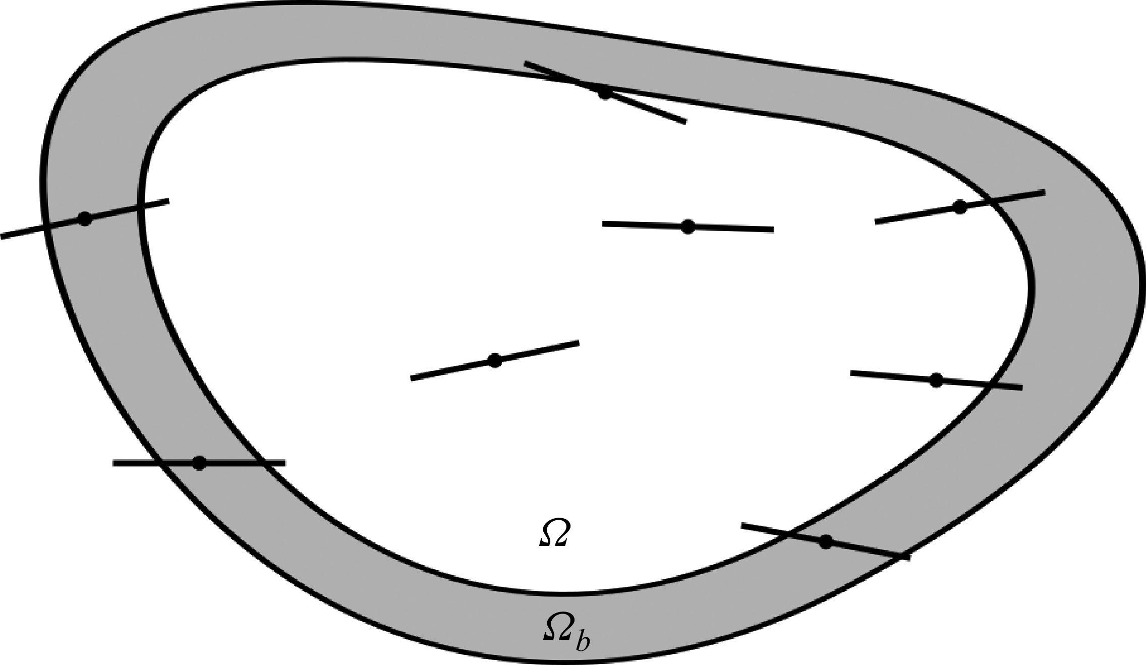


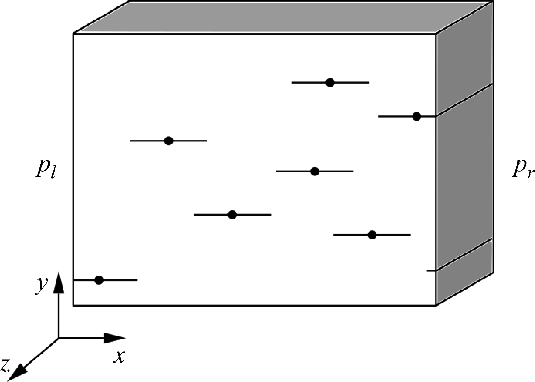


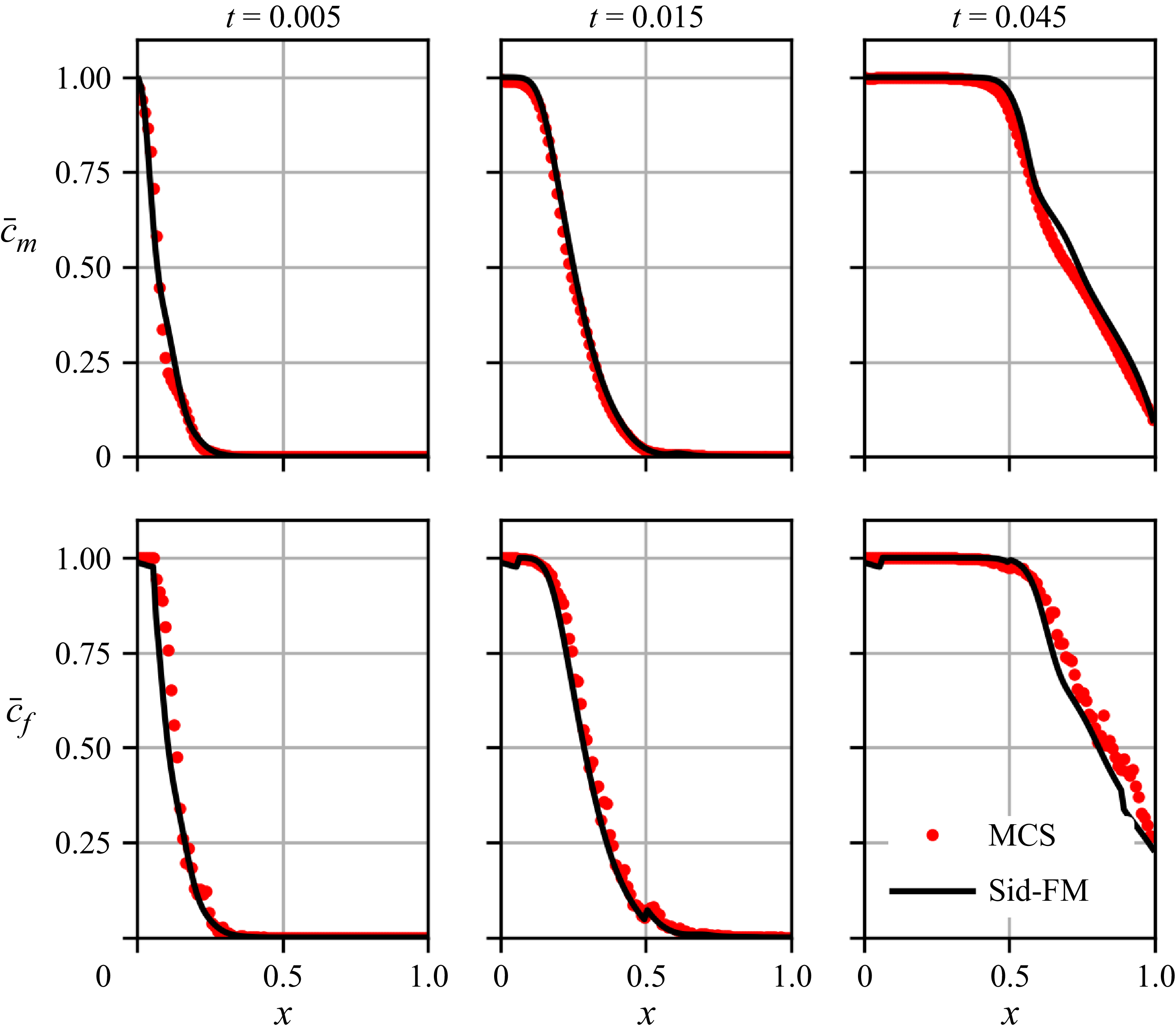


 Open access