


I. Introduction
The literature on the predictability of stock returns is voluminous, and the evidence on the predictability of index returns is an important part of this literature. Cochrane (Reference Cochrane2001) and Lettau and Ludvigson (Reference Lettau, Ludvigson, Ait-Sahalia and Hansen2010) conclude that a small fraction of the variation in monthly index returns can be predicted by variables such as the price-dividend ratio, the price-earnings and dividend payout ratios, short-term interest rates, and term and default spreads. Subsequent research has suggested additional predictors, such as the variance risk premium (Bollerslev, Tauchen, and Zhou (Reference Bollerslev, Tauchen and Zhou2009)), volatility of volatility (Huang, Schlag, Shaliastovich, and Thimme (Reference Huang, Schlag, Shaliastovich and Thimme2019)), and tail risk (Bollerslev and Todorov (Reference Bollerslev and Todorov2011), Andersen, Fusari, and Todorov (Reference Andersen, Fusari and Todorov2020)).
This article contributes to the literature on the predictability of market returns. However, rather than focus on predicting the returns on the market index, we start by investigating monthly returns on market volatility. Unlike volatility itself, which is highly persistent, we focus on realized returns on volatility based on positions in VIX futures contracts. We then investigate if these returns can be forecast using past data on VIX futures. This strategy is implementable in real time, similar to a strategy that attempts to forecast index returns using past index returns and index futures. Moreover, unlike the literature that uses variables such as price-dividend ratios to forecast index returns, we only rely on market prices measured at the same time, and we avoid the use of a low-frequency variable such as dividends.
It is well-known that average realized returns on market volatility are negative, indicating that a short volatility position is, on average, profitable, but that the return series contains large positive outliers. We confirm this result in our sample. We then use various reduced-form models of VIX dynamics to model VIX futures and expected returns on VIX futures contracts with different maturities and holding periods. Expected volatility returns on VIX futures are also negative on average and positively correlated with the time series of subsequent realized returns.
Because of the negative correlation between index returns and volatility and/or VIX, known as the leverage effect, our results also have implications for the predictability of (S&P 500) index returns. Specifically, the positive relation between expected volatility returns and realized subsequent volatility returns suggests that expected volatility returns negatively predict subsequent index returns. We find that our results on forecasting volatility returns indeed carry over to forecasting index returns, but the results from these predictive regressions are less statistically significant.
There is considerable debate in the literature about the evidence from predictive regressions, partly because the predictable component of 1-month returns is small. Several studies have advocated the use of predictive regressions using long-horizon returns to confirm the results of short-horizon regressions (Fama and French (Reference Fama and French1988), Cochrane (Reference Cochrane2001), (Reference Cochrane2011), and Bollerslev et al. (Reference Bollerslev, Tauchen and Zhou2009)). Specifically, in the presence of a persistent predictor, predictability of the 1-month return manifests itself in the pattern of regression slopes and $ {R}^2 $
s at longer horizons. We, therefore, not only report on predicting next-month realized volatility and index returns, but we also study the predictability of monthly VIX futures returns compounded over longer horizons, up to 5 years. We find that these predictive regressions indeed confirm our results. When we adopt the forward–backward predictive regressions of Bandi, Perron, Tamoni, and Tebaldi (Reference Bandi, Perron, Tamoni and Tebaldi2019), we obtain hump-shaped patterns in predictive
$ {R}^2 $
s at longer horizons. We, therefore, not only report on predicting next-month realized volatility and index returns, but we also study the predictability of monthly VIX futures returns compounded over longer horizons, up to 5 years. We find that these predictive regressions indeed confirm our results. When we adopt the forward–backward predictive regressions of Bandi, Perron, Tamoni, and Tebaldi (Reference Bandi, Perron, Tamoni and Tebaldi2019), we obtain hump-shaped patterns in predictive $ {R}^2 $
s for both realized volatility and index returns, with
$ {R}^2 $
s for both realized volatility and index returns, with $ {R}^2 $
s peaking at the 24-month horizon. This finding suggests the presence of different components in expected and realized volatility returns that operate at different frequencies. We cannot reject the null hypothesis of equilibrium generated predictability (EGP), which tests if the autocorrelation in the predictor is consistent with the pattern of the loadings of the predictive regressions as a function of the forecast horizon, as would be expected in an equilibrium setup (Eraker (Reference Eraker2025)).
$ {R}^2 $
s peaking at the 24-month horizon. This finding suggests the presence of different components in expected and realized volatility returns that operate at different frequencies. We cannot reject the null hypothesis of equilibrium generated predictability (EGP), which tests if the autocorrelation in the predictor is consistent with the pattern of the loadings of the predictive regressions as a function of the forecast horizon, as would be expected in an equilibrium setup (Eraker (Reference Eraker2025)).
Because the literature has shown that biases in predictive regressions (Stambaugh (Reference Stambaugh1999)) may worsen with longer horizons (Boudoukh, Israel, and Richardson (Reference Boudoukh, Israel and Richardson2022)), we show that biases in long-horizon predictive regressions for our application are very small compared to biases in forecasts based on the dividend-price ratio. These findings are consistent with Bollerslev, Marrone, Xu, and Zhou (Reference Bollerslev, Marrone, Xu and Zhou2014). We also provide evidence on the size and power properties of predictive regressions in finite samples based on parameterizations consistent with our empirical setup.
We demonstrate that our results are robust to a wide range of variations in the empirical setup, such as the implementation of the predictive regressions, the model for the VIX, the measure of expected returns, and the contract maturity. We also show that the expected volatility return retains predictive power in the presence of other predictors, such as the slope of the VIX term structure (Johnson (Reference Johnson2017)), the market variance risk premium, and variance-of-variance (Bollerslev et al. (Reference Bollerslev, Tauchen and Zhou2009)), and the tail factor (e.g., Bollerslev and Todorov (Reference Bollerslev and Todorov2011), Andersen, Fusari, and Todorov (Reference Andersen, Fusari and Todorov2015)). We use simple univariate sorts to demonstrate how the information in these predictors differs from the information in expected volatility returns, and we discuss the relation between our results and the findings of Cheng (Reference Cheng2018) on the VIX premium. Lastly, we show that return predictability can be further improved by using a predictor that combines expected volatility returns constructed from contracts with different maturities.
Aside from the literature on the predictability of market returns, our work is most closely related to the literature on market variance risk and the variance risk premium. Much of this literature focuses on measuring the market variance risk premium (Bakshi and Kapadia (Reference Bakshi and Kapadia2003a), Carr and Wu (Reference Carr and Wu2009), and Bondarenko (Reference Bondarenko2014)) as well as the variance risk premium on stocks and its relation to the market variance risk premium (Bakshi and Kapadia (Reference Bakshi and Kapadia2003b), Carr and Wu (Reference Carr and Wu2009), Driessen, Maenhout, and Vilkov (Reference Driessen, Maenhout and Vilkov2009), and Duarte, Jones, and Wang (Reference Duarte, Jones and Wang2024)). Martin (Reference Martin2017) studies the relation between the market variance risk premium and the market equity risk premium, while Bollerslev et al. (Reference Bollerslev, Tauchen and Zhou2009) and Pyun (Reference Pyun2019) study predictive regressions of the market risk premium on the variance risk premium. Like our article, Eraker and Wu (Reference Eraker and Wu2017) and Cheng (Reference Cheng2018) study returns on VIX futures. Cheng (Reference Cheng2018) focuses on the puzzle that the VIX premium does not increase with measures of risk. Eraker and Wu (Reference Eraker and Wu2017) analyze if the distribution of VIX futures returns is consistent with dynamic equilibrium. We instead focus on expected volatility returns and ask if they can predict realized volatility returns. We find that volatility risk is priced in VIX futures markets and that the price fluctuations correctly anticipate future market volatility returns and the corresponding S&P 500 returns. Moreover, the time series of expected volatility returns contains information that is distinct from several other risk measures suggested by theory and studies in the existing literature, such as the variance risk premium, tail risk, and the volatility of volatility.
The article proceeds as follows: Section II discusses the VIX futures data. Section III discusses the computation of realized and expected returns on volatility. Section IV presents the baseline empirical results. Section V discusses several extensions and robustness exercises, Section VI studies statistical biases in (long-horizon) predictive regressions, and Section VII concludes.
II. Data
We obtain daily VIX data from the Chicago Board Options Exchange (CBOE). In 1993, the CBOE developed the VXO volatility index, which was based on S&P 100 at-the-money options. In 2003, in light of structural changes in index option markets and advances in academic research, the CBOE refined the methodology and developed a new volatility index, the VIX, which is computed as a weighted average of S&P 500 option prices.Footnote 1
We download data on VIX futures from the CBOE website, which includes daily settlement prices, open and close prices, high and low prices, volume, and open interest. The sample period for the futures data is from Mar. 26, 2004, when futures contracts on the VIX were introduced and started trading, to Nov. 23, 2022. Our empirical analysis reports on futures contracts with different maturities. In the early part of the sample, there are typically four futures contracts listed every day. After October 2006, typically nine contracts are listed every day. We only include VIX futures contracts that expire on the Wednesday that is exactly 30 days prior to the third Friday of the following month. If that Wednesday or the Friday 30 days later is an exchange holiday, the VIX futures settle on Tuesdays instead.Footnote 2 Initially, VIX futures prices were quoted as the VIX times 10, and the contract multiplier was $100. Starting on Mar. 26, 2007, the CBOE Futures Exchange modified the contract specification by dividing futures prices by 10 and increasing the contract multiplier to $1,000, which brings the price in line with the underlying VIX index while leaving the contract size unchanged. We, therefore, rescale all futures prices prior to Mar. 26, 2007, accordingly. We apply several data filters. We require futures contracts to have valid settlement prices, positive volume, and positive open interest.
The sample period we use for the VIX index itself is longer, from Jan. 2, 1990, to Nov. 23, 2022, and we use daily data in estimation. Graph A of Figure 1 plots the VIX index for this period. The VIX index exhibits substantial variation over time and is strongly mean-reverting. In our sample period, it peaks at the start of the Covid-19 pandemic, closing at a historical high of 82.69 on Mar. 16, 2020. In the financial crisis, it reached a high of 80.96 on Nov. 20, 2008. Panel A of Table 1 reports summary statistics for the VIX for two sample periods: the January 1990 to November 2022 period, as well as March 2004 to November 2022, which corresponds to the period for which VIX futures data are available. The descriptive statistics are similar in these two samples, but the VIX has a slightly higher mean, smaller standard deviation, smaller (positive) skewness, and smaller kurtosis in the longer sample.
Graph A of Figure 1 plots the VIX. The sample period is from January 1990 to November 2022. Graph B plots daily prices of VIX futures with constant maturities of 1, 2, 3, 4, 5, 6, 7, 8, and 9 months. For each day in the sample, we use linear interpolation to generate these prices. The sample period is from Mar. 26, 2004 to Nov. 23, 2022.


Panel B of Table 1 reports summary statistics for VIX futures prices.Footnote 3 VIX futures prices are higher than the VIX on average, indicating that long investors pay a premium. Furthermore, VIX futures prices increase monotonically with maturity, from 20.20 for the 1-month contract to 22.35 for the 9-month contract. This upward-sloping term structure, often referred to as the contango trap, is the reason why rolling the VIX futures contract is associated with substantial losses (e.g., Whaley (Reference Whaley2013), Eraker and Wu (Reference Eraker and Wu2017)). Graph B of Figure 1 plots the evolution of the VIX futures term structure over the sample period. The shape of the term structure changes considerably over time. During normal times, VIX futures prices tend to be low and have an upward-sloping term structure. In times of market turbulence, such as during the financial crisis, the futures curve tends to increase and may become inverted or hump-shaped.
Graph A of Figure 2 reports the average daily trading volume and open interest per contract as a function of maturity. The majority of trading in VIX futures takes place at the short end of the term structure, with much larger volume and open interest for short-maturity contracts. Graph B shows the average daily trading volume and open interest per contract over time. The past decade has witnessed tremendous growth in the VIX futures market. The average daily volume per maturity was 33,390 contracts in 2018, more than 250 times higher than in 2004, and more than 50 times higher than in 2008.
Graph A of Figure 2 plots the average daily trading volume and open interest for VIX futures by time-to-maturity. Graph B plots the daily average trading volume and open interest per contract by year. The sample period is from Mar. 26, 2004 to Nov. 23, 2022.

III. Realized and Expected Returns on Volatility
We first compute ex post realized returns from investing in VIX futures for different investment horizons. We then discuss how to compute expected returns from holding VIX futures.
A. Realized Returns on Volatility
In this section, we analyze ex post realized returns from investing in VIX futures. Following the existing literature (e.g., Hong and Yogo (Reference Hong and Yogo2012), Singleton (Reference Singleton2013), and Cheng (Reference Cheng2018)), we measure the return on a futures contract as the return on a fully collateralized position.Footnote
4 Specifically, consider a VIX futures contract at time $ t $
that will expire at time
$ t $
that will expire at time $ T $
and currently trades at a price of
$ T $
and currently trades at a price of $ {F}_t(T) $
. The simple return
$ {F}_t(T) $
. The simple return $ {R}_{t,T} $
from holding this contract from time
$ {R}_{t,T} $
from holding this contract from time $ t $
to expiration is given by:
$ t $
to expiration is given by:
 $$ {R}_{t,T}=\frac{VIX_T}{F_t(T)}-1 $$
where $ {VIX}_T $
is the settlement value of the contract at maturity.Footnote
5 A long position in VIX futures provides a hedge against volatility risk because it has a positive payoff when the VIX increases. During our sample period, 219 VIX futures contracts matured. For each of these contracts, we establish a long position 1, 2, 3, 4, and 5 months prior to the expiration date and compute the corresponding hold-to-maturity returns.Footnote
6
$ {VIX}_T $
is the settlement value of the contract at maturity.Footnote
5 A long position in VIX futures provides a hedge against volatility risk because it has a positive payoff when the VIX increases. During our sample period, 219 VIX futures contracts matured. For each of these contracts, we establish a long position 1, 2, 3, 4, and 5 months prior to the expiration date and compute the corresponding hold-to-maturity returns.Footnote
6
Panel A of Table 2 reports the summary statistics for the resulting VIX futures returns.Footnote 7 To make the returns comparable, we scale all hold-to-maturity returns to monthly returns. Consistent with our observations on the term structure of VIX futures prices, the average returns to holding VIX futures are negative regardless of the horizon, which indicates that long investors, on average, pay a premium for buying VIX futures. Moreover, the average return decreases (in absolute value) as a function of time-to-maturity. Our finding that the volatility risk premium is negative and economically large, especially at short maturities, confirms existing evidence regarding the returns on market volatility, see, for instance, Andries, Eisenbach, Kahn, and Schmalz (Reference Andries, Eisenbach, Kahn and Schmalz2025), Cheng (Reference Cheng2018), Dew-Becker, Giglio, Le, and Rodriguez (Reference Dew-Becker, Giglio, Le and Rodriguez2017), and Eraker and Wu (Reference Eraker and Wu2017).

Panel A of Table 2 indicates that a long position in volatility using the 1-month contract incurs an average loss of −3.7% per month with an annualized Sharpe ratio of −0.405 over our sample period.Footnote 8 Graph A of Figure 3 plots the time series of 1-month hold-to-maturity VIX futures returns. The realized return on a long volatility position is negative most of the time, but occasionally it results in large positive payoffs. For example, in September 2008, during the financial crisis, a long position in a 1-month VIX futures contract resulted in a positive return of 120%. In March 2020 (the beginning of the Covid-19 pandemic), the return to a long position was 354%.
Graph A of Figure 3 plots monthly realized returns based on holding the 1-month VIX futures contract to maturity. Graph B plots expected 1-month hold-to-maturity VIX futures returns against the VIX. Graph C plots the expected returns from Graph B, together with subsequent 5-year VIX futures and stock returns.

Panel B of Table 2 provides additional insight into the term structure of volatility returns. We decompose the average 5-month hold-to-maturity return into five consecutive monthly holding period returns. Consider a VIX futures contract that expires in June (month t). We decompose the return of holding this contract from January to June (t – 5, t) into five monthly returns: January to February (t – 5, t – 4), February to March (t – 4, t – 3), March to April (t – 3, t – 2), April to May (t – 2, t – 1), and May to June (t – 1, t). Consistent with the findings in Panel A, Panel B shows that VIX futures have, on average, more negative returns when they are closer to maturity.
Panel C reports summary statistics for the 1-month holding period returns on VIX futures with different maturities. Each month $ t $
, we collect VIX futures that expire in month
$ t $
, we collect VIX futures that expire in month $ t+1 $
,
$ t+1 $
, $ t+2 $
,
$ t+2 $
, $ \dots $
,
$ \dots $
, $ t+5 $
, and we report on the monthly returns from holding those contracts from month
$ t+5 $
, and we report on the monthly returns from holding those contracts from month $ t $
to month
$ t $
to month $ t+1 $
. We establish a long position in VIX futures exactly 1 month prior to the futures expiration date in month
$ t+1 $
. We establish a long position in VIX futures exactly 1 month prior to the futures expiration date in month $ t+1 $
.Footnote
9 For the front contract, the resulting returns are identical to the 1-month holding-to-maturity returns analyzed in Panel A, with an average of −3.7%. For other maturities, these are monthly holding period returns. Consistent with our findings in Panels A and B, we find that the VIX futures holding period returns are, on average, negative and that they exhibit a strong negative relationship with maturity: The average return decreases monotonically from −3.7% for the 1-month contract to −0.4% for the 5-month contract. However, despite these differences, the holding period returns on VIX futures contracts are highly correlated across maturities. For example, the correlations between the return on the 1-month futures contract and the returns on 2-, 3-, 4-, and 5-month contracts are 0.95, 0.94, 0.93, and 0.92, respectively.
$ t+1 $
.Footnote
9 For the front contract, the resulting returns are identical to the 1-month holding-to-maturity returns analyzed in Panel A, with an average of −3.7%. For other maturities, these are monthly holding period returns. Consistent with our findings in Panels A and B, we find that the VIX futures holding period returns are, on average, negative and that they exhibit a strong negative relationship with maturity: The average return decreases monotonically from −3.7% for the 1-month contract to −0.4% for the 5-month contract. However, despite these differences, the holding period returns on VIX futures contracts are highly correlated across maturities. For example, the correlations between the return on the 1-month futures contract and the returns on 2-, 3-, 4-, and 5-month contracts are 0.95, 0.94, 0.93, and 0.92, respectively.
B. Computing Expected Returns on Volatility
We now discuss the computation of expected returns from holding VIX futures. This computation requires us to make some choices regarding implementation. First, note that the futures price $ {F}_t(T) $
is known at time
$ {F}_t(T) $
is known at time $ t $
and consider the conditional expectation of the return in equation (1):
$ t $
and consider the conditional expectation of the return in equation (1):
 $$ {ER}_{t,T}^V=\frac{E_t^P\left({VIX}_T\right)}{F_t(T)}-1. $$
where the superscript $ V $
indicates that this is a return on a long position in volatility, and the superscript
$ V $
indicates that this is a return on a long position in volatility, and the superscript $ P $
is used to denote the expectation under the physical measure. Equation (2) indicates that we need to make an assumption regarding the dynamics of the VIX under the physical measure.
$ P $
is used to denote the expectation under the physical measure. Equation (2) indicates that we need to make an assumption regarding the dynamics of the VIX under the physical measure.
Second, note that since the VIX itself is not tradable, the price of VIX futures cannot be pinned down by the cost of carry. However, no-arbitrage implies that the fair value of a VIX futures contract is the expected value of the VIX at maturity under the risk-neutral measure, $ {F}_t(T)={E}_t^Q\left({VIX}_T\right) $
, and therefore equation (2) can also be written as:
$ {F}_t(T)={E}_t^Q\left({VIX}_T\right) $
, and therefore equation (2) can also be written as:
 $$ {ER}_{t,T}^V=\frac{E_t^P\left({VIX}_T\right)}{F_t(T)}-1=\frac{E_t^P\left({VIX}_T\right)}{E_t^Q\left({VIX}_T\right)}-1. $$
Equation (3) indicates that the expected futures return can be computed using the observed futures price, or alternatively using a model for the VIX dynamic under the risk-neutral measure. We report results based on expected returns computed using the observed futures price.Footnote 10
C. The Dynamics of the VIX
Regardless of how we implement the denominator in equation (3), our empirical strategy requires the specification of a model for the VIX under the physical measure. We report results based on several models. First, consider a very simple model, which assumes that the VIX follows a square-root process under the physical measure:
 $$ {dVIX}_t=\kappa \left(\theta -{VIX}_t\right) dt+\sigma \sqrt{VIX_t} dW $$
where $ \theta $
is the long-run mean of the VIX and
$ \theta $
is the long-run mean of the VIX and $ \kappa $
is the mean-reversion parameter. Given this dynamic, the P-expectation in equation (3) is straightforward to compute:
$ \kappa $
is the mean-reversion parameter. Given this dynamic, the P-expectation in equation (3) is straightforward to compute:
 $$ {E}_t^P\left({VIX}_T\right)=\theta +\left({VIX}_t-\theta \right){e}^{-\kappa \left(T-t\right)}. $$
Given the mean-reverting property of the VIX in equation (4), the model states that the expected value of the future VIX is a weighted average of the long-run mean and the current VIX. This model is admittedly overly simplistic, and we, therefore, consider three alternative models for the VIX: the ARMA(2, 2) model used in Cheng (Reference Cheng2018), the heterogeneous autoregressive (HAR) model of Corsi (Reference Corsi2009) adapted for the VIX, where the predictors are the average VIX over the past month, week, and day, and finally a 2-factor model (e.g., Lee and Engle (Reference Lee and Engle1999), Alizadeh, Brandt, and Diebold (Reference Alizadeh, Brandt and Diebold2002), Engle and Rangel (Reference Engle and Rangel2008), and Christoffersen, Heston, and Jacobs (Reference Christoffersen, Heston and Jacobs2009)). This model assumes that the VIX mean reverts to a stochastic mean, which itself follows a square root process. Section A of the Suppementary Material provides more details on this model.
We start by comparing the performance of these four dynamics for forecasting VIX itself. We evaluate the models’ performance for three forecasting horizons: 1, 2, and 3 months ahead. Our implementation follows Bekaert and Hoerova (Reference Bekaert and Hoerova2014). Specifically, we divide the entire VIX sample (January 1990 to November 2022) into an in-sample period used to estimate the model parameters and an out-of-sample period used to evaluate forecasting performance. We consider three different sample splits: We use either 65%, 75%, and 85% of the data for estimating the parameters, and the remaining 35%, 25%, and 15% of the data are used for assessing out-of-sample forecasting performance.Footnote
11 As in Bekaert and Hoerova (Reference Bekaert and Hoerova2014), we estimate and evaluate the models using daily data, and the parameters are not updated in the out-of-sample period. We consider various performance measures, including the root mean squared error (RMSE), mean absolute error (MAE), the $ {R}^2 $
of the Mincer–Zarnowitz regression of realized VIX values onto forecasted values in the out-of-sample period, and the average correlation (Corr) between a given model’s forecast and the forecasts generated by the winning model based on each of the above three criteria. This latter measure provides insight into the economic proximity between different model forecasts.
$ {R}^2 $
of the Mincer–Zarnowitz regression of realized VIX values onto forecasted values in the out-of-sample period, and the average correlation (Corr) between a given model’s forecast and the forecasts generated by the winning model based on each of the above three criteria. This latter measure provides insight into the economic proximity between different model forecasts.
Table 3 reports the results, with Panels A, B, and C reporting on the 65–35, 75–25, and 85–15 sample splits, respectively, and Panel D reporting on the average performance across the three sample splits and the overall rankings. The overall rank is computed as the average rank across all four performance measures, with the best-performing model receiving a rank of 1 and the worst-performing model receiving a rank of 4.Footnote
12 Panel D indicates that for the purpose of forecasting the 1-month ahead VIX, the 1-factor model emerges as the best model overall, achieving an overall rank of 1.5 with the lowest RMSE, second-lowest MAE, and second-highest Mincer–Zarnowitz regression $ {R}^2 $
, and highest average correlation. For the purpose of forecasting the VIX 2 and 3 months ahead, the HAR model is the best overall performer, followed by the 1-factor model, the 2-factor model, and the ARMA(2,2) model. Unsurprisingly, the forecasting performance of all models drops significantly at 2- and 3-month horizons.
$ {R}^2 $
, and highest average correlation. For the purpose of forecasting the VIX 2 and 3 months ahead, the HAR model is the best overall performer, followed by the 1-factor model, the 2-factor model, and the ARMA(2,2) model. Unsurprisingly, the forecasting performance of all models drops significantly at 2- and 3-month horizons.

We conclude that a clearly superior model does not emerge from this forecast comparison. Relatedly, the differences in model forecasting performance are relatively small in several dimensions. Rather than report on (a different) best-performing model for every forecast horizon, we therefore use the same model in our baseline analysis, and report on the other models in the robustness analysis in Section V.D. For simplicity, we use the 1-factor model as the baseline model.
IV. Forecasting Volatility Returns and S&P 500 Returns
We first report our baseline results on forecasting volatility returns, and then our baseline results on forecasting S&P 500 returns, both based on the 1-month contract. Next, we report on returns for contracts with longer maturities.
A. Forecasting Realized Volatility Returns
We first discuss the details of the implementation of the expected volatility return used in our baseline analysis. We estimate the VIX dynamics and expected returns recursively using an expanding window to ensure there is no look-ahead bias.Footnote
13 At each time $ t $
, we use VIX data from January 1990 up to time
$ t $
, we use VIX data from January 1990 up to time $ t $
to estimate the parameters of the model in equation (4) via maximum likelihood by exploiting the fact that the transition density of the square-root process is available in closed form (Pearson and Sun (Reference Pearson and Sun1994)). Section A of the Supplementary Material provides additional details on the estimation of the 1-factor model and the time-series properties of the VIX. We then use those parameters and equation (5) to compute the physical 1-month expectation of the VIX index. Together with the 1-month futures prices, this allows us to compute the 1-month expected volatility return at time
$ t $
to estimate the parameters of the model in equation (4) via maximum likelihood by exploiting the fact that the transition density of the square-root process is available in closed form (Pearson and Sun (Reference Pearson and Sun1994)). Section A of the Supplementary Material provides additional details on the estimation of the 1-factor model and the time-series properties of the VIX. We then use those parameters and equation (5) to compute the physical 1-month expectation of the VIX index. Together with the 1-month futures prices, this allows us to compute the 1-month expected volatility return at time $ t $
, (
$ t $
, ( $ {ER}_{t,t+1}^V $
).Footnote
14
$ {ER}_{t,t+1}^V $
).Footnote
14
The solid red line in Graphs B and C of Figure 3 plots the resulting time series of 1-month hold-to-maturity expected returns on VIX futures using the square root model. Compared to the realized returns in Graph A, the time series of expected returns is more persistent. Graph B also plots the time series of the (squared) VIX.Footnote 15 The expected return becomes more negative following sharp increases in volatility. The scatterplot of the VIX against the baseline expected volatility returns in Graph A of Figure 4 confirms this pattern. Note that this stylized fact is related to but distinct from the one investigated by Moreira and Muir (Reference Moreira and Muir2017), (Reference Moreira and Muir2019), who document that the risk-adjusted return to a long S&P 500 position is lower following spikes in volatility.
Figure 4 plots the VIX and subsequent 5-year VIX futures returns against expected volatility returns. Graph A scatterplots the VIX against expected volatility returns. Graphs B and C scatterplot expected returns against realized returns. Graph C highlights the role of the financial crisis.

Our baseline analysis uses these expected returns in forecasting regressions to predict future realized returns on the 1-month VIX futures contract for different return horizons. The literature on forecasting index, stock, and bond returns indicates that it may be beneficial to examine forecasting regressions at both short and long horizons, in the sense that the patterns in the regression coefficients and $ {R}^2 $
s for the long-horizon regressions can be used to confirm the results of short-horizon regressions (see, for instance, Fama and French (Reference Fama and French1988), Cochrane (Reference Cochrane2001), (Reference Cochrane2011), Cochrane and Piazzesi (Reference Cochrane and Piazzesi2005), Bollerslev et al. (Reference Bollerslev, Tauchen and Zhou2009), (Reference Bollerslev, Marrone, Xu and Zhou2014), and Kostakis, Magdalinos, and Stamatogiannis (Reference Kostakis, Magdalinos and Stamatogiannis2015)).Footnote
16 We, therefore, not only consider predicting next-month realized returns, but we also study the predictability of monthly VIX futures returns compounded over longer horizons, up to 5 years (60 months), scaled by the forecast horizon. Specifically, we construct a time series of
$ {R}^2 $
s for the long-horizon regressions can be used to confirm the results of short-horizon regressions (see, for instance, Fama and French (Reference Fama and French1988), Cochrane (Reference Cochrane2001), (Reference Cochrane2011), Cochrane and Piazzesi (Reference Cochrane and Piazzesi2005), Bollerslev et al. (Reference Bollerslev, Tauchen and Zhou2009), (Reference Bollerslev, Marrone, Xu and Zhou2014), and Kostakis, Magdalinos, and Stamatogiannis (Reference Kostakis, Magdalinos and Stamatogiannis2015)).Footnote
16 We, therefore, not only consider predicting next-month realized returns, but we also study the predictability of monthly VIX futures returns compounded over longer horizons, up to 5 years (60 months), scaled by the forecast horizon. Specifically, we construct a time series of $ h $
-month futures returns, and we report on
$ h $
-month futures returns, and we report on $ h=1,3,6,12,..\dots \dots, 60 $
. These predictive regressions are thus given by:
$ h=1,3,6,12,..\dots \dots, 60 $
. These predictive regressions are thus given by:
 $$ \frac{1}{h}\sum \limits_{i=1}^h{r}_{t,t+i}^{VIX}={\alpha}_{t+h}+{\beta}_{t+h}{ER}_{t,t+1}^V+{\epsilon}_{t+h},h=\mathrm{1,3,6,12},\dots, 60 $$
where $ h $
is the index for the time horizon (in months),
$ h $
is the index for the time horizon (in months), $ {\sum}_{i=1}^h{r}_{t,t+i}^{VIX} $
is the cumulative future log return from holding VIX futures over the horizon
$ {\sum}_{i=1}^h{r}_{t,t+i}^{VIX} $
is the cumulative future log return from holding VIX futures over the horizon $ h $
calculated by summing up the monthly realized log returns from Graph A in Figure 3, and
$ h $
calculated by summing up the monthly realized log returns from Graph A in Figure 3, and $ {ER}_{t,t+1}^V $
is the expected (log) return from holding 1-month VIX futures to maturity. We estimate a single forecasting regression for each horizon (i.e., for a given forecast horizon
$ {ER}_{t,t+1}^V $
is the expected (log) return from holding 1-month VIX futures to maturity. We estimate a single forecasting regression for each horizon (i.e., for a given forecast horizon $ h $
, the regression in equation (6) is estimated once). An alternative approach is to estimate a different forecasting regression at each time
$ h $
, the regression in equation (6) is estimated once). An alternative approach is to estimate a different forecasting regression at each time $ t $
and report on the average slopes and
$ t $
and report on the average slopes and $ {R}^2 $
s of these regressions. We report this alternative implementation in Section V.C.
$ {R}^2 $
s of these regressions. We report this alternative implementation in Section V.C.
Panel A of Table 4 reports the results. The literature has emphasized potential statistical problems with overlapping returns in long-horizon regressions. We discuss these issues in Section VI. Table 4 reports t-statistics according to Hansen and Hodrick (Reference Hansen and Hodrick1980) and Hodrick (Reference Hodrick1992), because our findings in Section VI confirm existing results that these t-statistics have better small-sample properties in the presence of overlapping returns compared to OLS or Newey–West t-statistics.Footnote 17

The slope coefficients are positive at all horizons. The t-statistics are U-shaped as a function of the forecast horizon. The pattern across horizons differs somewhat between the Hodrick and Hansen–Hodrick t-statistics, but both indicate statistical significance at multiple horizons. The $ {R}^2 $
are much higher for long forecast horizons. As discussed by Cochrane (Reference Cochrane2001), for example,
$ {R}^2 $
are much higher for long forecast horizons. As discussed by Cochrane (Reference Cochrane2001), for example, $ {R}^2 $
s mechanically increase as a function of the forecast horizon in forecasting regressions with persistent regressors, provided that the loading on the predictor is nonzero to start with. The point estimate of the loadings decreases as a function of the horizon, consistent with a predictor that is mean-reverting. The pattern at long horizons is consistent with the first-order sample autocorrelation of 0.85 for an AR(1) predictor.Footnote
18
$ {R}^2 $
s mechanically increase as a function of the forecast horizon in forecasting regressions with persistent regressors, provided that the loading on the predictor is nonzero to start with. The point estimate of the loadings decreases as a function of the horizon, consistent with a predictor that is mean-reverting. The pattern at long horizons is consistent with the first-order sample autocorrelation of 0.85 for an AR(1) predictor.Footnote
18
To provide additional intuition for the results in Table 4 and the high $ {R}^2 $
s at long horizons, Graph B of Figure 4 scatterplots the baseline expected volatility returns against subsequent 5-year realized returns on VIX futures. We focus on long-horizon returns in these plots because they are less variable, which leads to a higher
$ {R}^2 $
s at long horizons, Graph B of Figure 4 scatterplots the baseline expected volatility returns against subsequent 5-year realized returns on VIX futures. We focus on long-horizon returns in these plots because they are less variable, which leads to a higher $ {R}^2 $
and therefore a scatterplot that makes the relation with expected returns easier to gauge. More negative 1-month expected returns anticipate multi-year lower (more negative) subsequent returns on VIX futures. Graph C of Figure 3 plots the corresponding time series of the 1-month expected returns
$ {R}^2 $
and therefore a scatterplot that makes the relation with expected returns easier to gauge. More negative 1-month expected returns anticipate multi-year lower (more negative) subsequent returns on VIX futures. Graph C of Figure 3 plots the corresponding time series of the 1-month expected returns $ {x}_{t,t+1} $
along with the subsequent 5-year realized returns on VIX futures.Footnote
19
$ {x}_{t,t+1} $
along with the subsequent 5-year realized returns on VIX futures.Footnote
19
A potential concern is that our sample is relatively short. The financial crisis and the subsequent shock to returns represent a major event in this short sample. The same is true for the Covid-19 crisis, but presumably its effect on subsequent (long-horizon) returns is only partially realized as yet in our sample. We, therefore, need to be especially careful, because the variation in long-horizon returns and the resulting predictability might be largely due to this single event. Graph C of Figure 4 shows that this is not the case. We scatterplot 5-year realized returns against expected returns and distinguish between returns that overlap with the financial crisis (in blue) and those that do not (in red). Clearly, the positive relation between expected and subsequently realized returns is present in both subsamples.
In summary, we document that expected volatility returns are statistically and economically significant predictors of realized returns on VIX futures. Next, we discuss the relation between these findings and the existing literature on the predictability of S&P 500 index returns.
B. Forecasting S&P 500 Index Returns
The leverage effect refers to the negative correlation between (index) returns and innovations to (market) variance. The economic mechanism behind this negative correlation is strongly debated, but there is consensus about the stylized fact. Usually, this correlation is measured using daily, weekly, or monthly returns. We report the correlation between returns to holding the S&P 500 and the 1-month VIX futures contract as a function of the time horizon. Panel C of Table 4 shows that this stylized fact also obtains for longer return horizons and that the magnitude of the correlation is remarkably constant across horizons. The correlations between the two returns are highly negative and range from −0.76 to −0.85.
We, therefore, conjecture that the finding in Section IV.A. that expected returns can predict realized VIX futures returns may have implications for predicting index returns. To test this hypothesis, we use the baseline expected returns to predict subsequent index returns over different horizons:
 $$ \frac{1}{h}\sum \limits_{i=1}^h{r}_{t,t+i}^{SP}={\alpha}_{t+h}+{\beta}_{t+h}{ER}_{t,t+1}^V+{\epsilon}_{t+h},h=\mathrm{1,3,6,12},\dots, 60 $$
where $ {\sum}_{i=1}^h{r}_{t,t+i}^{SP} $
denotes the log index return over horizon
$ {\sum}_{i=1}^h{r}_{t,t+i}^{SP} $
denotes the log index return over horizon $ h $
, and
$ h $
, and $ {ER}_{t,t+1}^V $
again is the baseline 1-month log expected volatility return.
$ {ER}_{t,t+1}^V $
again is the baseline 1-month log expected volatility return.
Panel D of Table 4 summarizes the results using the baseline implementation. Index returns are from CRSP. Consistent with our conjecture, expected returns on volatility indeed contain predictive information about future index returns. Specifically, the expected volatility returns negatively predict index returns, and the predictive patterns mirror those in the volatility return predictive regressions in Panel A. However, on average across horizons, the statistical significance and the $ {R}^2 $
s are lower compared to the volatility returns in Panel A.Footnote
20 Another difference is that for these predictive regressions, the Hodrick t-statistics are generally a bit higher than the HH t-statistics. Graph C of Figure 3 plots the subsequent 5-year S&P 500 index returns (the broken red line) together with the expected volatility return and the subsequent 5-year VIX futures return. The plot visually confirms the high correlations between the three time series.
$ {R}^2 $
s are lower compared to the volatility returns in Panel A.Footnote
20 Another difference is that for these predictive regressions, the Hodrick t-statistics are generally a bit higher than the HH t-statistics. Graph C of Figure 3 plots the subsequent 5-year S&P 500 index returns (the broken red line) together with the expected volatility return and the subsequent 5-year VIX futures return. The plot visually confirms the high correlations between the three time series.
C. Forecasting the Returns on Longer-Maturity VIX Futures Contracts
Section IV.A reports on predictive regressions using the returns on the 1-month VIX futures contract. Table 5 instead reports on predictive regressions based on monthly returns on the 2-, 3-, 4-, and 5-month VIX futures contracts compounded to longer horizons. Panel C of Table 2 reports descriptive statistics for these returns.

For completeness, we repeat the results for the 1-month contract from Table 4. The results for the 1-month contract generalize to other maturities. For example, at the 3-year forecast horizon, the expected volatility return significantly predicts the returns to 2-, 3-, 4-, and 5-month contracts, with $ {R}^2 $
s of
$ {R}^2 $
s of $ 39.9\% $
,
$ 39.9\% $
, $ 29.63\% $
,
$ 29.63\% $
, $ 26.39\% $
, and
$ 26.39\% $
, and $ 26.03\% $
respectively. This is not surprising because of the high correlations between VIX futures returns on contracts with different maturities discussed in Section III.A. Also unsurprisingly, the loadings of the forecasting regressions are more stable across forecast horizons for contracts with longer maturities. Overall, the
$ 26.03\% $
respectively. This is not surprising because of the high correlations between VIX futures returns on contracts with different maturities discussed in Section III.A. Also unsurprisingly, the loadings of the forecasting regressions are more stable across forecast horizons for contracts with longer maturities. Overall, the $ {R}^2 $
s of the predictive regressions are somewhat higher for shorter-maturity contracts.
$ {R}^2 $
s of the predictive regressions are somewhat higher for shorter-maturity contracts.
V. Alternative Predictors and Robustness Analysis
In this section, we present robustness results and explore how our results are related to the evidence in the existing literature, which almost exclusively considers predictive regressions for returns on the S&P 500. First, we present results from univariate sorts. We then consider the predictive power of expected volatility returns in the presence of predictors used in the existing literature. We also investigate the robustness of our results with respect to the computation of expected returns and the implementation of the predictive regressions. We first report on results where we recursively estimate the predictive regressions. Next, we use alternative models for the dynamics of the VIX to compute expected returns, and we use a predictor that combines the information in futures contracts with different maturities. Finally, we further explore the term structure of return predictability using the forward–backward aggregation approach of Bandi et al. (Reference Bandi, Perron, Tamoni and Tebaldi2019) and we test whether the term structure of return predictability is consistent with the persistence of the expected volatility returns (Eraker (Reference Eraker2025)).
A. Univariate Sorts on Expected Returns
Simple (univariate) sorts can be useful to illustrate nonlinear relationships in the data. We sort the 219 monthly expected volatility returns used in Panel A of Table 4 and depicted in Graph B of Figure 3 into three groups/portfolios. Panel B of Table 4 reports the average subsequent VIX futures returns for tercile portfolios sorted by the expected volatility return. We use the baseline implementation with the 1-month VIX futures contract and the expected volatility return from the 1-factor model. Once again, we study not only realized returns over the following month but also longer horizon returns. Consistent with the returns in the predictive regressions, we divide the $ h $
-month log returns by
$ h $
-month log returns by $ h $
. The long–short returns are statistically significant at all horizons. They are economically large, especially at short horizons. The signs of the long–short returns are consistent with the signs of the loadings in the predictive regressions.
$ h $
. The long–short returns are statistically significant at all horizons. They are economically large, especially at short horizons. The signs of the long–short returns are consistent with the signs of the loadings in the predictive regressions.
B. Predicting Variance Returns with Alternative Predictors
Table 6 presents the results of univariate and bivariate predictive regressions of the S&P 500 and volatility returns on the expected volatility return and other predictors. Once again, these results are based on the baseline implementation with the 1-month VIX futures contract and the expected volatility return from the 1-factor model. We do not think of these results as a horse race. The expected volatility return in equation (2) is suggested by theory as a natural predictor for future market volatility returns and, by extension, for index returns. This connection to theory is less direct for several other predictors used in the literature. A high correlation between any such predictor and the expected volatility returns, therefore, does not reduce the relevance of the expected volatility return as a novel predictor; instead, it merely illustrates its connection to the existing empirical literature. Panel C of Table 1 reports the correlations between the expected volatility return and these predictors of S&P 500 returns that have been studied in the existing literature. The absolute value of this correlation is highest for the VIX term structure slope.

Tables A2 and A3 in the Supplementary Material report univariate results for multiple forecasting horizons. Results are, of course, somewhat dependent on the forecasting horizon, because the predictive power and statistical significance of different predictors peak at different horizons. To give the alternative predictors their best chance, Table 6 reports on an intermediate (3-year) return horizon. The overall conclusion is that the predictive power of the expected volatility returns remains in the presence of other predictors. We now discuss these results in more detail.
1. The Variance Risk Premium
We remarked earlier that expected volatility returns become more negative when volatility increases. This may be related to the findings of Bollerslev et al. (Reference Bollerslev, Tauchen and Zhou2009) that the market variance risk premium has predictive power for index returns. We therefore document the predictive power of the variance risk premium for subsequent S&P 500 index returns and VIX futures returns in our sample. We adopt the definition of the variance risk premium in Bollerslev et al. (Reference Bollerslev, Tauchen and Zhou2009), $ {VIX}_{t,t+1}^2-{RV}_{t-1,t} $
, where
$ {VIX}_{t,t+1}^2-{RV}_{t-1,t} $
, where $ {RV}_{t-1,t} $
denotes the realized variance between
$ {RV}_{t-1,t} $
denotes the realized variance between $ t-1 $
and
$ t-1 $
and $ t $
, and we express the variance risk premium in monthly percentage-squared terms. The sample for realized variance and hence the variance risk premium ends in December 2020.
$ t $
, and we express the variance risk premium in monthly percentage-squared terms. The sample for realized variance and hence the variance risk premium ends in December 2020.
Table A3 in the Supplementary Material confirms the robustness of the finding in Bollerslev et al. (Reference Bollerslev, Tauchen and Zhou2009) that the variance risk premium positively predicts index returns, and Table A2 in the Supplementary Material confirms our prior that this predictive power also obtains for volatility returns because of the leverage effect.Footnote 21 Table 6 indicates that for the purpose of predicting index returns and volatility returns, the information in the expected volatility return differs from that in the variance risk premium.
2. Decomposing the Variance Risk Premium
Bandi and Perron (Reference Bandi and Perron2008) and Sizova (Reference Sizova2013) report that lagged variance predicts index returns. Bandi et al. (Reference Bandi, Perron, Tamoni and Tebaldi2019) report a hump-shaped pattern in forward–backward regressions, with a maximum $ {R}^2 $
at the 16-year horizon. The lagged variance is one of the two components of the implementation of the variance risk premium in Bollerslev et al. (Reference Bollerslev, Tauchen and Zhou2009). We, therefore, report on predictive regressions using both components of the variance risk premium.Footnote
22 Following the construction of the variance risk premium, the realized variance and the squared VIX are also expressed in monthly percentage-squared terms. The sample for the VIX ends in November 2022. The sample for realized variance ends in December 2020.
$ {R}^2 $
at the 16-year horizon. The lagged variance is one of the two components of the implementation of the variance risk premium in Bollerslev et al. (Reference Bollerslev, Tauchen and Zhou2009). We, therefore, report on predictive regressions using both components of the variance risk premium.Footnote
22 Following the construction of the variance risk premium, the realized variance and the squared VIX are also expressed in monthly percentage-squared terms. The sample for the VIX ends in November 2022. The sample for realized variance ends in December 2020.
Tables A2 and A3 in the Supplementary Material show that the risk-neutral and physical variances have some (long-horizon) predictive power by themselves. In Tables A2 (A3) in the Supplementary Material, the slope estimates are negative (positive) for both variance measures for all return horizons. For a given maturity, the loadings are also very similar for both variances, while the $ {R}^2s $
are slightly higher for the risk-neutral variance. Table 6 shows that the predictive ability of the expected volatility return remains in the presence of the realized variance or the squared VIX.
$ {R}^2s $
are slightly higher for the risk-neutral variance. Table 6 shows that the predictive ability of the expected volatility return remains in the presence of the realized variance or the squared VIX.
3. The Variance Risk Premium and the Volatility Return
Next, we rewrite the volatility return in equation (1) as:
 $$ {R}_{t,T}=\frac{VIX_T-{F}_t(T)}{F_t(T)}. $$
Comparing this return with the variance risk premium, we see that the expected volatility return differs from the variance risk premium in (at least) three ways: i) It uses volatility rather than variance units; ii) The second term in the numerator is the futures price rather than the realized variance; and iii) The volatility return in equation (8) is scaled by the futures price. To further investigate the relation to the variance risk premium, Tables A2 and A3 in the Supplementary Material, therefore, document the predictive power of the nonscaled predictor $ {VIX}_T-{F}_t(T) $
. While the slope of course differs from the baseline results in Table 4, the patterns in the t-statistics and
$ {VIX}_T-{F}_t(T) $
. While the slope of course differs from the baseline results in Table 4, the patterns in the t-statistics and $ {R}^2 $
s are similar. Row 5, labeled “Scaled VRP,” reports on the variance risk premium divided by the futures price as a predictor. These results are more similar to those obtained for the VRP. We conclude that the expected volatility return contains information that is distinct from the variance risk premium.
$ {R}^2 $
s are similar. Row 5, labeled “Scaled VRP,” reports on the variance risk premium divided by the futures price as a predictor. These results are more similar to those obtained for the VRP. We conclude that the expected volatility return contains information that is distinct from the variance risk premium.
4. Volatility of Volatility
The higher moments of the return distribution capture risk that is different from the variance. We, therefore, also study if volatility of volatility can predict future returns. Following Huang et al. (Reference Huang, Schlag, Shaliastovich and Thimme2019), to measure volatility of volatility, we use the VVIX index, which is calculated from VIX options in an analogous way to the VIX index. We obtain VVIX data from August 2006 to November 2022 from the CBOE website. Tables A2 and A3 in the Supplementary Material indicate that the VVIX has some predictive power, mainly for intermediate horizons. The pattern of the $ {R}^2s $
and t-statistics as a function of the forecast horizon for VVIX differs from the pattern for expected volatility returns in our sample, but also from the patterns for the VIX and the VRP. Table 6 once again indicates that including this variable does not affect the predictive power of the expected volatility return.
$ {R}^2s $
and t-statistics as a function of the forecast horizon for VVIX differs from the pattern for expected volatility returns in our sample, but also from the patterns for the VIX and the VRP. Table 6 once again indicates that including this variable does not affect the predictive power of the expected volatility return.
5. The Tail Factor
Recent studies have highlighted the importance of tail risk.Footnote 23 We obtain data on the Left Tail Volatility index (LTV) from tailindex.com. LTV is a measure of return volatility generated by the left tail of the 1-week risk-neutral return distribution, inferred from short-maturity out-of-the-money put options. Tables A2 and A3 in the Supplementary Material indicate that LTV is informative about future returns, especially at longer horizons. In both tables, the sign at the 1-month horizon differs from the sign for all other horizons, but it is not statistically significant. The bivariate regression in Table 6 shows that the predictive power of the expected volatility return remains.
6. The VIX Slope
Johnson (Reference Johnson2017) finds that the second principal component of the VIX term structure (the slope factor) contains predictive information about future returns on a range of volatility assets, including variance swaps, VIX futures, and straddles at the daily and monthly horizons. For example, he finds that the slope predicts VIX futures returns at the monthly horizon with an $ {R}^2 $
of 11.44%. We confirm these results for our sample. We obtain the slope factor data from Travis Johnson’s website. The sample for the slope factor ends in December 2017. Although our returns are measured differently from Johnson (Reference Johnson2017), Tables A2 and A3 in the Supplementary Material confirm that the slope factor predicts VIX futures returns and show that this also translates into index return predictability. The predictive power for futures returns peaks at the 3-year horizon with an
$ {R}^2 $
of 11.44%. We confirm these results for our sample. We obtain the slope factor data from Travis Johnson’s website. The sample for the slope factor ends in December 2017. Although our returns are measured differently from Johnson (Reference Johnson2017), Tables A2 and A3 in the Supplementary Material confirm that the slope factor predicts VIX futures returns and show that this also translates into index return predictability. The predictive power for futures returns peaks at the 3-year horizon with an $ {R}^2 $
of 23%. The bivariate regression in Table 6 shows that the t-statistics for both regressors are smaller compared to the univariate regressions, which is not surprising given that the correlation between the two predictors is −0.63. However, the predictive power of the expected volatility return remains when including the VIX slope in the predictive regression.
$ {R}^2 $
of 23%. The bivariate regression in Table 6 shows that the t-statistics for both regressors are smaller compared to the univariate regressions, which is not surprising given that the correlation between the two predictors is −0.63. However, the predictive power of the expected volatility return remains when including the VIX slope in the predictive regression.
7. Univariate Sorts
Univariate sorts are also useful to illustrate the similarities and differences between the informational content in expected volatility returns and other forecasting variables. Panels A–C of Table A5 in the Supplementary Material report on tercile portfolios sorted by the variance risk premium, the VVIX, and LTV. The signs of the long–short returns are mostly consistent with the predictive regressions, but for the VRP, the return at the 1-month horizon is almost zero and not significant. We verified that the sign is often negative in subsamples, while the sign for longer horizons is positive. This finding is related to Cheng (Reference Cheng2018), who refers to it as the VIX premium puzzle. Similar to the expected volatility returns, the return difference for the variance risk premium is highly statistically significant at longer horizons.
Table A5 in the Supplementary Material also confirms that the information in the VVIX differs from that in expected returns and the VRP because the economically largest and statistically most significant return spreads occur at intermediate horizons. For LTV, the sign at the 1-month horizon also differs from that at longer horizons, and the long–short returns are largest at intermediate horizons.
8. Summary
In summary, Table A3 in the Supplementary Material confirms that predictors suggested by the existing literature have some predictive power for S&P 500 index returns, and Table A2 in the Supplementary Material shows that this translates into predictive power for volatility returns. However, Table 6 suggests that the expected volatility return seems to contain different or additional information, and therefore retains predictive power for realized volatility returns and S&P 500 index returns when these other predictors are included in the predictive regression.
C. Out-of-Sample Recursive Predictive Regressions
Our baseline implementation does not suffer from data-snooping because expected returns are computed recursively, that is, we construct the expected return predictor by re-estimating the VIX model parameters each month. However, for simplicity, we present results based on a single forecasting regression. We now report on predictive regressions using the same expected returns, but with re-estimating the predictive regression each period. Panel B of Tables 7 and 8 reports the average slope estimates, t-statistics, and $ {R}^2s $
from these predictive regressions as a function of the forecast horizon. The literature often refers to these recursive regressions as out-of-sample predictive regressions, while our baseline results, which are repeated in Panel A of Tables 7 and 8 for convenience, are referred to as in-sample predictive regressions.
$ {R}^2s $
from these predictive regressions as a function of the forecast horizon. The literature often refers to these recursive regressions as out-of-sample predictive regressions, while our baseline results, which are repeated in Panel A of Tables 7 and 8 for convenience, are referred to as in-sample predictive regressions.


Tables 7 and 8 indicate that the impact on the results is limited. Figure 5 provides more details by plotting the resulting time series of the regression slopes, $ {R}^2 $
s, and t-statistics. Graphs A, C, and E report on the 1-month horizon and Graphs B, D, and F on the 5-year horizon. By construction, the time series for the 5-year returns is shorter. For a given forecast horizon, the slopes and
$ {R}^2 $
s, and t-statistics. Graphs A, C, and E report on the 1-month horizon and Graphs B, D, and F on the 5-year horizon. By construction, the time series for the 5-year returns is shorter. For a given forecast horizon, the slopes and $ {R}^2 $
s over time are of a similar order of magnitude, and do not seem to be affected by outliers. However, the slopes and especially the
$ {R}^2 $
s over time are of a similar order of magnitude, and do not seem to be affected by outliers. However, the slopes and especially the $ {R}^2 $
s decrease toward the end of the sample period, perhaps due to the impact of the Covid-19 crisis on volatility returns. Panels E and F present the time series of t-statistics in the recursive regressions. Note the strong pattern in the Hodrick t-statistics in Panel F, in contrast with the pattern in the HH t-statistics, suggesting potential biases in the Hodrick t-statistics when using long horizons in small samples. In Section VI, we present simulation evidence that is consistent with these patterns.
$ {R}^2 $
s decrease toward the end of the sample period, perhaps due to the impact of the Covid-19 crisis on volatility returns. Panels E and F present the time series of t-statistics in the recursive regressions. Note the strong pattern in the Hodrick t-statistics in Panel F, in contrast with the pattern in the HH t-statistics, suggesting potential biases in the Hodrick t-statistics when using long horizons in small samples. In Section VI, we present simulation evidence that is consistent with these patterns.
Graphs A, C, and E of Figure 5 report on the 1-month horizon and Graphs B, D, and F on the 60-month horizon. Graphs A–B report on the slope, Graphs C–D on the $ {R}^2 $
, and Graphs E–F on the t-statistics for out-of-sample (recursive) predictive regressions with 1-month VIX futures returns.
$ {R}^2 $
, and Graphs E–F on the t-statistics for out-of-sample (recursive) predictive regressions with 1-month VIX futures returns.

D. VIX Dynamics and Predictive Regressions
In Section III.C, we compare the predictive performance of four different VIX dynamics for the future VIX: a simple square root specification, a 2-factor generalization of this simple model, an ARMA(2,2) specification, and the heterogeneous autoregressive (HAR) model of Corsi (Reference Corsi2009).Footnote 24 We find that no model clearly dominates, and that the models’ predictive performance displays more similarities than differences. We have, therefore, reported results based on the simplest model, the square root specification for the VIX. We now present the results of predictive regressions for volatility returns on the 1-month contract for the three other models.
We focus on an ARMA(2,2) dynamic because Cheng (Reference Cheng2018) uses ARMA dynamics for the VIX and mainly reports results based on an ARMA(2,2) dynamic.Footnote 25 The main focus in Cheng (Reference Cheng2018) is the puzzle that the ex ante estimate of the VIX premium embedded in VIX futures falls or stays flat when risk rises. This ex ante risk premium is a measure of the expected return on volatility. Despite this VIX premium puzzle, Cheng (Reference Cheng2018) finds that estimated risk premiums reliably forecast future 1-month premiums, similar to our finding that expected returns on volatility forecast realized returns. Cheng (Reference Cheng2018), (Reference Cheng2020) analyze realized 1-month volatility returns, while we also study long-horizon returns.
Panels C–E of Table 7 report on predictive regressions for forecasting VIX futures returns. As in the baseline analysis, all expected return measures are based on the recursive implementation in which we estimate volatility forecasting models recursively to generate the numerator. The results are qualitatively similar to the baseline results in Panel A, but the $ {R}^2s $
are generally lower, especially at long horizons. Panels C–E of Table 8 present the corresponding results for forecasting S&P 500 returns. Again, they are qualitatively similar to the baseline results.
$ {R}^2s $
are generally lower, especially at long horizons. Panels C–E of Table 8 present the corresponding results for forecasting S&P 500 returns. Again, they are qualitatively similar to the baseline results.
E. Simple Returns
Cochrane (Reference Cochrane2001) shows that when predicting index returns using the price-dividend ratio, results for log returns and simple returns are different at long horizons. Panel F of Table 7 reports results for predicting simple rather than log VIX futures returns, and Panel F of Table 8 reports on simple S&P 500 returns. In both cases, the results are similar to the baseline results in Panel A.Footnote 26
F. Combining Expected Returns Across Maturities
Cochrane and Piazzesi (Reference Cochrane and Piazzesi2005) show that a simple combination of forward rates predicts excess bond returns. Motivated by their results, we investigate whether combining expected volatility returns across maturities can improve forecasting performance. Similar to computing expected 1-month holding-to-maturity returns ( $ {ER}_{t,t+1}^V $
), each month we can also compute the expected returns from holding a 2-month (
$ {ER}_{t,t+1}^V $
), each month we can also compute the expected returns from holding a 2-month ( $ {ER}_{t,t+2}^V $
), 3-month (
$ {ER}_{t,t+2}^V $
), 3-month ( $ {ER}_{t,t+3}^V $
), 4-month (
$ {ER}_{t,t+3}^V $
), 4-month ( $ {ER}_{t,t+4}^V $
), and 5-month VIX futures contract (
$ {ER}_{t,t+4}^V $
), and 5-month VIX futures contract ( $ {ER}_{t,t+5}^V $
) to maturity by using market prices of 2-, 3-, 4-, and 5-month contracts and the baseline VIX forecasting model to compute the corresponding physical expectations. We then extract the first principal component of these expected returns across different maturities and use it to predict the returns on (1-month) VIX futures and the S&P 500 index.Footnote
27
$ {ER}_{t,t+5}^V $
) to maturity by using market prices of 2-, 3-, 4-, and 5-month contracts and the baseline VIX forecasting model to compute the corresponding physical expectations. We then extract the first principal component of these expected returns across different maturities and use it to predict the returns on (1-month) VIX futures and the S&P 500 index.Footnote
27
Panel G of Tables 7 and (8) reports the results for forecasting VIX futures (S&P 500 index) returns. We find that combining expected returns across maturities in general leads to a notable increase in the $ {R}^2 $
of the predictive regressions, especially for VIX futures. For example, when using the first common component to predict returns, for the 24-month forecast horizon, the
$ {R}^2 $
of the predictive regressions, especially for VIX futures. For example, when using the first common component to predict returns, for the 24-month forecast horizon, the $ {R}^2 $
is
$ {R}^2 $
is $ 30.14\% $
and
$ 30.14\% $
and $ 11.59\% $
for VIX futures and the S&P 500 index, respectively, as compared to
$ 11.59\% $
for VIX futures and the S&P 500 index, respectively, as compared to $ 17.07\% $
and
$ 17.07\% $
and $ 5.13\% $
for the baseline expected return reported in Panel A.Footnote
28
$ 5.13\% $
for the baseline expected return reported in Panel A.Footnote
28
G. Forward–Backward Regressions
This section further explores the term structure of volatility return predictability. We once again use our baseline predictive regression setup with the 1-month futures contract and the simple square-root 1-factor model to construct the expected volatility return. We implement the forward–backward regressions of Bandi et al. (Reference Bandi, Perron, Tamoni and Tebaldi2019), who regress long-horizon returns (which are aggregated forward) on long-run past expected volatility returns (which are aggregated backward), as follows:
 $$ {r}_{t+1,t+h}={\alpha}_h+{\beta}_h{ER}_{t-h+1,t}^V+\epsilon $$
where $ {r}_{t+1,t+h} $
is the long run VIX futures or S&P 500 index (log) return over different future horizons indexed by
$ {r}_{t+1,t+h} $
is the long run VIX futures or S&P 500 index (log) return over different future horizons indexed by $ h $
, and
$ h $
, and $ {ER}_{t-h+1,t}^V $
is the sum of the expected volatility returns over the past
$ {ER}_{t-h+1,t}^V $
is the sum of the expected volatility returns over the past $ h $
months. Long-horizon forward–backward regressions capture information that cannot be captured by the classical long-horizon regressions in Tables 4 and 5, where the loadings and
$ h $
months. Long-horizon forward–backward regressions capture information that cannot be captured by the classical long-horizon regressions in Tables 4 and 5, where the loadings and $ {R}^2 $
s mechanically increase with horizon in the presence of persistent regressors. This approach can also be used to identify components of the predictor that operate at different frequencies, thereby overcoming low signal-to-noise problems in the predictive regression.
$ {R}^2 $
s mechanically increase with horizon in the presence of persistent regressors. This approach can also be used to identify components of the predictor that operate at different frequencies, thereby overcoming low signal-to-noise problems in the predictive regression.
Panel A of Table 9 reports the results for forecasting VIX futures returns and Panel B for S&P 500 index returns. Consistent with the findings reported in Bandi et al. (Reference Bandi, Perron, Tamoni and Tebaldi2019) for predictive regressions of market returns on variance, we observe hump-shaped patterns in predictability in both panels. Estimates are statistically significant at horizons less than or equal to 24 months.Footnote
29 Graph A of Figure 6 plots the $ {R}^2 $
s of the backward–forward regressions as a function of the horizon. The
$ {R}^2 $
s of the backward–forward regressions as a function of the horizon. The $ {R}^2 $
s peak at the 24-month horizon for both predictive regressions. These findings suggest the presence of different components in expected and realized volatility returns that operate at different frequencies. Note that these results are not inconsistent with the patterns we document in Tables 4 and 5, because those results do not rely on backward aggregation.
$ {R}^2 $
s peak at the 24-month horizon for both predictive regressions. These findings suggest the presence of different components in expected and realized volatility returns that operate at different frequencies. Note that these results are not inconsistent with the patterns we document in Tables 4 and 5, because those results do not rely on backward aggregation.

Graph A of Figure 6 plots the $ {R}^2 $
s of the forward–backward regressions in Bandi et al. (Reference Bandi, Perron, Tamoni and Tebaldi2019) as a function of the aggregation horizon. Graph B plots the equilibrium and realized slopes used in the EGP test of Eraker (Reference Eraker2025) as a function of the horizon. Results are based on the baseline 1-factor model and the VIX futures contract with a 1-month maturity.
$ {R}^2 $
s of the forward–backward regressions in Bandi et al. (Reference Bandi, Perron, Tamoni and Tebaldi2019) as a function of the aggregation horizon. Graph B plots the equilibrium and realized slopes used in the EGP test of Eraker (Reference Eraker2025) as a function of the horizon. Results are based on the baseline 1-factor model and the VIX futures contract with a 1-month maturity.

H. Equilibrium Generated Predictability
Eraker (Reference Eraker2025) proposes a test of EGP. The intuition behind the test is that in an equilibrium setup, the autocorrelation in the predictor ought to be related to the pattern of the loadings of the predictive regression as a function of the forecast horizon. We follow Eraker (Reference Eraker2025) and report on the following $ Q $
statistic:
$ Q $
statistic:
 $$ Q={\left(\hat{b}-{b}^{\ast}\right)}^{\prime}\hat{\Omega}\left(\hat{b}-{b}^{\ast}\right) $$
where $ \hat{b} $
is the vector of estimated slopes from OLS regressions of future 1-month VIX futures returns on the expected volatility return,
$ \hat{b} $
is the vector of estimated slopes from OLS regressions of future 1-month VIX futures returns on the expected volatility return, $ {b}^{\ast } $
is the vector of corresponding theory-implied slopes, and
$ {b}^{\ast } $
is the vector of corresponding theory-implied slopes, and $ \hat{\Omega} $
is the estimated variance–covariance matrix. Specifically, the
$ \hat{\Omega} $
is the estimated variance–covariance matrix. Specifically, the $ {\hat{b}}_h $
are estimated using the following regressions:
$ {\hat{b}}_h $
are estimated using the following regressions:
 $$ {r}_{t+h-1,t+h}={\alpha}_h+{b}_h{ER}_t^V+\epsilon \hskip1em h=1,2,\dots \mathrm{60} $$
where $ {r}_{t+h-1,t+h} $
is the one-period return on VIX futures
$ {r}_{t+h-1,t+h} $
is the one-period return on VIX futures $ h $
months from now.Footnote
30 The theory-implied slopes are computed from the contemporaneous regression of VIX futures returns on the changes in the expected volatility return, under the assumption that the expected return follows an AR(1) process, that is:
$ h $
months from now.Footnote
30 The theory-implied slopes are computed from the contemporaneous regression of VIX futures returns on the changes in the expected volatility return, under the assumption that the expected return follows an AR(1) process, that is:
 $$ {r}_t={\alpha}_0+{b}_0\Delta {ER}_t^V+\epsilon $$
 $$ {ER}_t^V=\rho {ER}_{t-1}^V+{u}_t. $$
We find that $ {b}_0 $
is negative, consistent with the notion that a positive shock to expected returns is associated with a price decrease and hence a lower contemporaneous realized return. A negative
$ {b}_0 $
is negative, consistent with the notion that a positive shock to expected returns is associated with a price decrease and hence a lower contemporaneous realized return. A negative $ {b}_0 $
implies that the implied slopes
$ {b}_0 $
implies that the implied slopes $ {b}^{\ast } $
are positive, since
$ {b}^{\ast } $
are positive, since $ {b}_h^{\ast }={b}_0\left({\rho}^h-{\rho}^{h-1}\right) $
.
$ {b}_h^{\ast }={b}_0\left({\rho}^h-{\rho}^{h-1}\right) $
.
Graph B of Figure 6 plots the realized one-period slopes together with theory-implied slopes. The one-period estimated slopes are mostly positive, suggesting that expected volatility returns are positively related to future VIX futures returns. However, they turn negative around the 4-year horizon, which explains the decrease in the $ {R}^2 $
s at the 4-year horizon observed in Table 4. As mentioned previously, the theory-implied slopes are always positive and decrease with the horizon.
$ {R}^2 $
s at the 4-year horizon observed in Table 4. As mentioned previously, the theory-implied slopes are always positive and decrease with the horizon.
Panel C of Table 9 reports the $ Q $
statistics for different horizons
$ Q $
statistics for different horizons $ h $
as well as the associated p values, based on the statistic’s
$ h $
as well as the associated p values, based on the statistic’s $ {\chi}^2 $
distribution with
$ {\chi}^2 $
distribution with $ h-1 $
degrees of freedom. For example, when
$ h-1 $
degrees of freedom. For example, when $ h=12 $
, we use the first 12 one-period slopes to compute the
$ h=12 $
, we use the first 12 one-period slopes to compute the $ Q $
statistic. The results suggest that the EGP null hypothesis cannot be rejected across horizons. For instance, when we use the entire term structure (i.e.,
$ Q $
statistic. The results suggest that the EGP null hypothesis cannot be rejected across horizons. For instance, when we use the entire term structure (i.e., $ h=60 $
), the
$ h=60 $
), the $ Q $
statistic is 51.868 with a p value of 0.734. Panel D reports the same test for forecasting S&P 500 index returns and finds that the EGP null cannot be rejected either.Footnote
31
$ Q $
statistic is 51.868 with a p value of 0.734. Panel D reports the same test for forecasting S&P 500 index returns and finds that the EGP null cannot be rejected either.Footnote
31
VI. Inference in Long-Horizon Volatility Return Regressions
It is well known that predictive regressions can induce statistical biases, and the literature has recognized that these biases may be further compounded in long-horizon predictive regressions with overlapping returns. In this section, we investigate these biases in the context of our data and sample, and we study size and power based on the parameterization of the predictive regressions.
A. Bias in OLS Slopes in Predictive Regressions
It is well known that forecasting with a persistent predictor may induce biases, even when returns are not overlapping (Stambaugh (Reference Stambaugh1986), (Reference Stambaugh1999)). Furthermore, there is an extensive literature on potential problems with long-horizon forecasting regressions with overlapping returns. We now discuss how these issues impact our empirical results. For clarity, we repeat our baseline forecasting regression:
 $$ \frac{1}{h}\sum \limits_{i=1}^h{r}_{t,t+i}={\alpha}_{t+h}+{\beta}_{t+h}{ER}_{t,t+1}^V+{\epsilon}_{t+h},h=\mathrm{1,3,6,12},\dots, 60 $$
where $ {r}_{t,t+i} $
is the log return from holding VIX futures or the S&P 500 index for different horizons indexed by
$ {r}_{t,t+i} $
is the log return from holding VIX futures or the S&P 500 index for different horizons indexed by $ i $
, and
$ i $
, and $ {ER}_{t,t+1}^V $
is the expected log volatility return.
$ {ER}_{t,t+1}^V $
is the expected log volatility return.
The seminal work by Stambaugh (Reference Stambaugh1986), (Reference Stambaugh1999) discusses biases in the slope estimate in the single-period predictive regression when the predictor is persistent, and its innovations are correlated with returns, and provides a plug-in adjustment for the biases based on the Kendall (Reference Kendall1954) approximation. The literature has long recognized that these biases may also be present and may be further compounded in long-horizon predictive regressions with overlapping returns. Recently, Boudoukh, Israel, and Richardson (Reference Boudoukh, Israel and Richardson2022) (henceforth BIR) show how to compute the equivalent of the Stambaugh bias in the slope estimates for the case of long horizon regressions. We apply the BIR correction to our predictive regressions with expected volatility returns. Note that the BIR correction reduces to the Stambaugh correction in the special case of the one-period (1-month) horizon.
Panel A of Table 10 compares the bias-adjusted slopes of the predictive regressions according to BIR with the unadjusted slopes based on the baseline measure of expected returns in Table 4. The OLS slope estimates in Panel A of Table 4 are slightly biased upward when predicting VIX futures returns, because the innovations to expected returns are slightly negatively correlated with the innovations to realized volatility returns. For the index return predictability regressions, Panel B of Table 10 indicates that the OLS estimate in Panel D of Table 4 is slightly biased downward due to the positive correlation between the innovations to expected returns and index returns.

These biases in the OLS slope coefficients are very small in our setting, mainly because the expected volatility return is much less persistent than the dividend price ratio, which is used in BIR to quantify biases.Footnote 32 Bollerslev et al. (Reference Bollerslev, Marrone, Xu and Zhou2014) reach a similar conclusion regarding the bias when using the VRP as a predictor. For expected volatility returns, another factor is that the correlation between the innovations to the predictor and the forecasting regression is small in magnitude.Footnote 33
B. Comparing Standard Errors
Another potential problem with long-horizon regressions is the computation of the standard errors. In our baseline analysis, we report Hansen and Hodrick (Reference Hansen and Hodrick1980) and Hodrick (Reference Hodrick1992) standard errors to account for the overlapping nature of the data because we found that these approaches have the best statistical properties. Panel C of Table 10 compares these standard errors with OLS standard errors. We also report on Newey and West (Reference Newey and West1987) standard errors, with lag length equal to the number of overlapping observations.Footnote 34 These standard errors are often used in the literature on predictive regressions. The OLS and Newey–West t-statistics are clearly much higher than the Hansen–Hodrick and Hodrick t-statistics. In Panel D, we report the results of the weighted least squares (WLS) approach in Johnson (Reference Johnson2018) applied to the volatility forecasting regressions. We follow Johnson (Reference Johnson2018) and use the squared return as a proxy for conditional variance. Panel D shows that the slope and t-statistics change substantially at short and medium horizons, but at 3, 4, and 5-year horizons, the results are very similar to the OLS results. This is intuitive because at short horizons the conditional return variance is likely to fluctuate substantially, whereas the conditional variance does not move that much at longer horizons, and the results for WLS and OLS are similar.
C. Size and Power in Predictive Regressions
A large literature documents that the finite sample distribution of predictive regression statistics can be very different from the asymptotic distribution and the evidence for stock return predictability becomes much weaker or statistically insignificant when taking into account the small sample size of long horizon regressions and the use of overlapping returns (see, among others, Goetzmann and Jorion (Reference Goetzmann and Jorion1993), Nelson and Kim (Reference Nelson and Kim1993), Kirby (Reference Kirby1997), Boudoukh, Richardson, and Whitelaw (Reference Boudoukh, Richardson and Whitelaw2008)). In this section, we use simulations to investigate if our findings can be attributed to small sample bias. We simulate 219 monthly returns on VIX futures under the assumption of no predictability and an AR(1) process for our baseline measure of expected volatility return $ {x}_t $
:
$ {x}_t $
:
 $$ {r}_{t+1}^{VIX}={\overline{r}}^{VIX}+{v}_{t+1} $$
 $$ {x}_{t+1}=c+\rho {x}_t+{u}_{t+1} $$
where $ {\overline{r}}^{VIX} $
is the mean return of 1-month VIX futures,
$ {\overline{r}}^{VIX} $
is the mean return of 1-month VIX futures, $ {v}_{t+1} $
and
$ {v}_{t+1} $
and $ {u}_{t+1} $
are shocks.Footnote
35 We then use the simulated data to estimate the regression of
$ {u}_{t+1} $
are shocks.Footnote
35 We then use the simulated data to estimate the regression of $ {\sum}_{i=1}^h{r}_{t+i}^{VIX} $
on
$ {\sum}_{i=1}^h{r}_{t+i}^{VIX} $
on $ {x}_t $
over different horizons, as in our actual empirical analysis, and record the slope coefficient, various t-statistics, and
$ {x}_t $
over different horizons, as in our actual empirical analysis, and record the slope coefficient, various t-statistics, and $ {R}^2 $
. We repeat this 50,000 times to construct a finite sample distribution of slope coefficients, t-statistics, and
$ {R}^2 $
. We repeat this 50,000 times to construct a finite sample distribution of slope coefficients, t-statistics, and $ {R}^2 $
s. This is a standard framework for testing against the null of no predictability in the predictability literature.Footnote
36
$ {R}^2 $
s. This is a standard framework for testing against the null of no predictability in the predictability literature.Footnote
36
Graph A of Figure 7 compares the empirical slopes (data) with the mean and 95th percentile of the finite sample distribution of the slope, based on the parameterization of the predictive regression with the baseline expected volatility return. The mean of the simulated slope estimates exceeds zero across all horizons, suggesting that slope coefficients are biased upward in our case.Footnote 37 However, the mean slope in the simulation is very close to the truth (zero), thereby confirming the very small BIR bias slope corrections in Table 10. These results also confirm that the BIR correction formula works well. Most importantly, comparing the empirical slopes with the 95th percentile shows that the empirical slope coefficients are statistically significant at the 5% level at most horizons.
Graph A of Figure 7 plots the slope coefficients in predictive regressions for volatility returns. We compare the slope coefficients from the data with the mean and 95th percentile of their finite sample distribution under the null of no predictability. Graph B plots the $ {R}^2 $
from the data with the mean and 95th percentile of the finite sample distribution under the null of no predictability. Graph C plots the 95th percentile of the finite sample distribution of various t-statistics under the null of no predictability. The null hypothesis is parameterized using the baseline expected volatility returns.
$ {R}^2 $
from the data with the mean and 95th percentile of the finite sample distribution under the null of no predictability. Graph C plots the 95th percentile of the finite sample distribution of various t-statistics under the null of no predictability. The null hypothesis is parameterized using the baseline expected volatility returns.

Graph B of Figure 7 compares the $ {R}^2 $
found in the data, with the mean and 95th percentile of the simulated
$ {R}^2 $
found in the data, with the mean and 95th percentile of the simulated $ {R}^2 $
across 50,000 simulated samples. Consistent with existing studies, we find that in predictive regressions with overlapping returns and a persistent predictor,
$ {R}^2 $
across 50,000 simulated samples. Consistent with existing studies, we find that in predictive regressions with overlapping returns and a persistent predictor, $ {R}^2 $
s increase with the horizon, even if there is no predictability (see also Bollerslev et al. (Reference Bollerslev, Marrone, Xu and Zhou2014)). However, the high
$ {R}^2 $
s increase with the horizon, even if there is no predictability (see also Bollerslev et al. (Reference Bollerslev, Marrone, Xu and Zhou2014)). However, the high $ {R}^2 $
s in our predictive regressions are significant at most horizons and cannot be entirely explained by small sample bias at longer horizons. For example, the mean and 95th percentile of
$ {R}^2 $
s in our predictive regressions are significant at most horizons and cannot be entirely explained by small sample bias at longer horizons. For example, the mean and 95th percentile of $ {R}^2 $
under the null of no predictability are 4.49% and 17.93%, respectively, for the 3-year horizon, whereas the corresponding
$ {R}^2 $
under the null of no predictability are 4.49% and 17.93%, respectively, for the 3-year horizon, whereas the corresponding $ {R}^2 $
in the data is 33.57%.
$ {R}^2 $
in the data is 33.57%.
We now turn to the size properties of the t-statistics documented in Table 10. Graph C of Figure 7 plots the 95th percentile of various t-statistics across 50,000 simulated samples, indicating the size properties of different standard errors in finite samples. Consistent with existing studies, we find that the t-statistics are biased upward in finite samples. At the 1-month horizon, the bias in the t-statistics does not appear to be all that severe: The 95% critical values of the sampling distribution of all t-statistics are close to 1.645 (1.664 for OLS, 1.671 for HH, 1.693 for Hodrick, and 1.693 for NW). It becomes progressively worse, however, as we move to longer horizons. For example, at the 4-year horizon, OLS (NW) t-statistics above 5.637 (3.176) are observed in 5% of all simulated samples, indicating that there is a serious size distortion and that OLS and NW t-statistics tend to reject the null hypothesis far too often in finite samples. HH and Hodrick t-statistics perform better, although they also have the incorrect size. At the 4-year horizon, the corresponding 95% critical values of HH and Hodrick t-statistics are 2.110 and 2.0670, respectively. Comparing the 95th percentile values to the corresponding t-statistics we found in the data (Table 10), we find that empirical t-statistics are significant across the majority of horizons, and therefore, the statistical evidence against the null of no predictability cannot be entirely explained by small sample bias. Finally, the Hodrick t-statistics are closest to the asymptotic values for most horizons, except for very long horizons, where HH t-statistics are most reliable.
We also conduct an analysis of the power of different t-statistics to examine their performance when the null hypothesis of no predictability is false. Section C of the Supplementary Material reports the results. The performance ranking of the various t-statistics is less clear for power than for size, and depends on the parameterization.
In summary, we confirm the presence of statistical biases in predictive regressions with long-horizon returns. However, for our application, the Stambaugh bias (and the BIR extension to long horizons) is very small for all reasonable parameterizations. We confirm results in the existing literature that HH and Hodrick standard errors have better finite sample size properties for our empirical exercise. The relative ranking of various standard errors based on power depends on the parameterization of the forecasting regression.
VII. Conclusion
We use the information in VIX futures prices to study realized and expected returns on market volatility. Expected volatility returns on VIX futures are available in closed form. We compute realized monthly returns on volatility based on fully collateralized positions in VIX futures contracts and investigate if these returns can be forecast using the ex ante expected returns.
Expected volatility returns positively predict subsequent realized volatility returns. Volatility returns are negative on average. Following increases in volatility, expected volatility returns and subsequent realized volatility returns become more negative. We confirm our results using predictive regressions with long-horizon returns. Our results also have implications for the predictability of index returns. Because of the negative correlation between index returns and volatility returns, expected volatility returns negatively predict subsequent index returns, but these results are statistically less significant.
Our predictability results are robust to a wide range of variations in the empirical setup and to a number of important statistical concerns. The predictive power of expected returns remains when controlling for other predictors, such as the slope of the VIX term structure in Johnson (Reference Johnson2017), a tail factor estimated from index options (Andersen et al. (Reference Andersen, Fusari and Todorov2015)), the market variance (Bandi and Perron (Reference Bandi and Perron2008), Bandi et al. (Reference Bandi, Perron, Tamoni and Tebaldi2019)), and the market variance risk premium (Bollerslev et al. (Reference Bollerslev, Tauchen and Zhou2009)).
Supplementary Material
To view supplementary material for this article, please visit http://doi.org/10.1017/S0022109026102683.









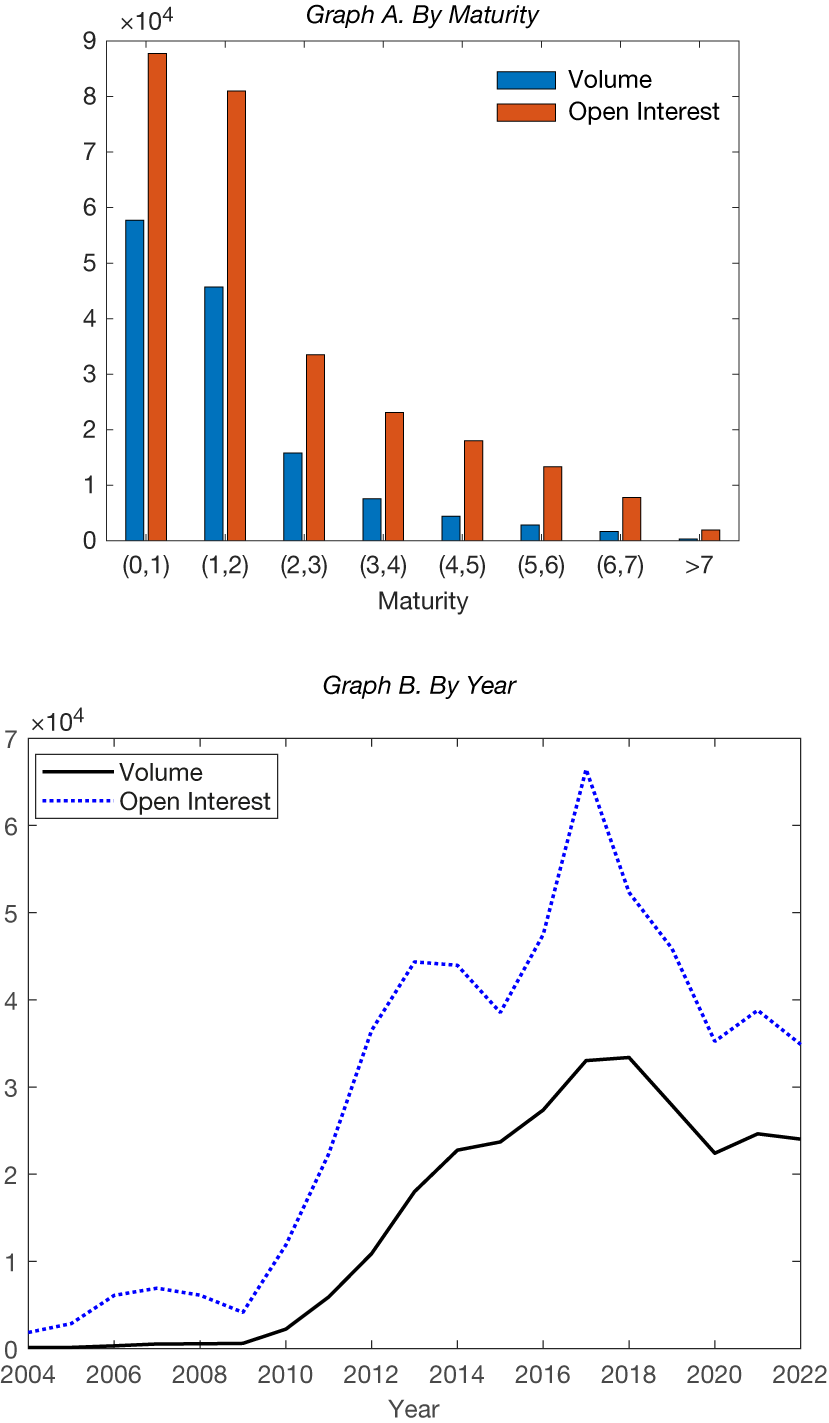


 Open access

