


1. Introduction
Turbulent boundary layers (TBLs), such as those found on the surfaces of aircraft, underwater vehicles, turbines and propeller blades, are ubiquitous in engineering systems. A TBL comprises an inner layer and an outer layer. The inner layer is responsible for most of the growth of the velocity from the wall value to the free stream value. As a result, inner layer modelling has garnered considerable attention, as evidenced by numerous prior studies (Piomelli & Balaras Reference Piomelli and Balaras2002; Kalitzin et al. Reference Kalitzin, Medic, Iaccarino and Durbin2005; Smits, McKeon & Marusic Reference Smits, McKeon and Marusic2011; Bose & Park Reference Bose and Park2018; Marusic & Monty Reference Marusic and Monty2019). Current models of the inner layer, including the wall treatments in Reynolds-averaged Navier–Stokes (RANS) models and large-eddy simulation (LES) wall models, are based on the following law of the wall (LoW) (Prandtl Reference Prandtl1925; Marusic et al. Reference Marusic, Monty, Hultmark and Smits2013):
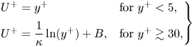 \begin{equation} \left.
\begin{array}{ll@{}} U^+ = y^+ & \text{for}\ y^+<5 ,\\
U^+ = \dfrac{1}{\kappa}\ln(y^+)+B, & \text{for}\ y^+\gtrsim
30, \end{array} \right\}
\end{equation}
\begin{equation} \left.
\begin{array}{ll@{}} U^+ = y^+ & \text{for}\ y^+<5 ,\\
U^+ = \dfrac{1}{\kappa}\ln(y^+)+B, & \text{for}\ y^+\gtrsim
30, \end{array} \right\}
\end{equation}
where  $U$ is the mean streamwise velocity; the superscript + denotes normalization by the wall units, $u_\tau \equiv \sqrt {\tau _w/\rho }$ and $\delta _\nu \equiv \nu /u_\tau$; $\tau _w$ is the wall-shear stress; $\rho$ is the fluid density; $\nu$ is the kinematic viscosity; $\kappa \approx 0.4$ is the von Kármán constant; and $B\approx 5$ is a constant. The coordinate system is such that $x$ is the streamwise direction, $y$ is the wall-normal direction and $z$ is the transverse direction.
Take the algebraic equilibrium wall model (EWM) as an example. The model relies on the LoW in (1.1) to compute the wall-shear stress as a function of the velocity at a distance from the wall (Bou-Zeid, Meneveau & Parlange Reference Bou-Zeid, Meneveau and Parlange2005; Yang, Park & Moin Reference Yang, Park and Moin2017):
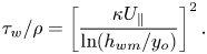 \begin{equation} \tau_w/\rho=\left[\frac{\kappa U_{\|}}{\ln(h_{wm}/y_o)}\right]^2. \end{equation}
Here,  $U_{\|}$ is the wall-parallel velocity at a distance $h_{wm}$ from the wall, and $y_o$ is a viscous/roughness length scale. Another example is the Spalart–Allmaras (SA) model (Spalart & Allmaras Reference Spalart and Allmaras1992), which is calibrated such that it is consistent with the following eddy viscosity scaling:
 \begin{equation} \nu_t=\kappa y u_\tau D, \end{equation}
where  $D$ is a damping function. While inner-layer models like the ones highlighted above are extensively used in computational fluid dynamics, the LoW itself is, in principle, valid under equilibrium conditions only. As a result, LoW-based models are, strictly speaking, valid under equilibrium conditions only.
Previous studies have noted the limitations of the LoW and the models derived from it. Studies such as those by Chen et al. (Reference Chen, Wu, Griffin, Shi and Yang2023), among others (Bobke et al. Reference Bobke, Vinuesa, Örlü and Schlatter2017; Parthasarathy & Saxton-Fox Reference Parthasarathy and Saxton-Fox2023), highlighted history effects, demonstrating that the velocity profiles in a pressure-gradient (PG) TBL depend not only on the state of the local flow but also on the history of the pressure gradient. For instance, imposing a favourable pressure gradient causes the flow to accelerate. In this process, the turbulent production and the wall-shear stress increase. However, it takes time before their values become those found in a statistically steady flow. As another example, Rota et al. (Reference Rota, Monti, Rosti and Quadrio2023) and Scarselli et al. (Reference Scarselli, Lopez, Varshney and Hof2023) reported that under a special pulsatile driving force, turbulence will diminish even when the Reynolds number is above the transition value.
The presence of such history effects limits the log law's effectiveness in approximating the mean flow in the presence of pressure gradient forces. Recent work by Hansen, Yang & Abkar (Reference Hansen, Yang and Abkar2023) and Lozano-Durán et al. (Reference Lozano-Durán, Giometto, Park and Moin2020) reported poor performance of the LoW-based EWM in a three-dimensional boundary layer. Recognizing these deficiencies, efforts have been made to enhance the LoW and its associated models (Kays, Crawford & Weigand Reference Kays, Crawford and Weigand2004; Knopp Reference Knopp2014; Knopp et al. Reference Knopp, Buchmann, Schanz, Eisfeld, Cierpka, Hain, Schröder and Kähler2015; Park & Moin Reference Park and Moin2014; Yang et al. Reference Yang, Sadique, Mittal and Meneveau2015; Huang, Yang & Kunz Reference Huang, Yang and Kunz2019; Yang et al. Reference Yang, Xia, Lee, Lv and Yuan2020; Huang & Yang Reference Huang and Yang2021; Fowler, Zaki & Meneveau Reference Fowler, Zaki and Meneveau2022; Hansen et al. Reference Hansen, Yang and Abkar2023; Subrahmanyam et al. Reference Subrahmanyam, Xu, Cantwell and Alonso2023). Here, we review some of these studies. Kays et al. (Reference Kays, Crawford and Weigand2004) compiled existing data and proposed the following empirical damping function:
 \begin{equation} D_k=1-\exp\left(-{y^+}/{A^+_k}\right), A^+_k=\frac{25.0}{c\mathcal{P}^++1}, \end{equation}
where  $\mathcal {P^+}$ denotes the local pressure gradient (normalized with the wall shear stress $\tau _w$ and the wall length $\delta _\nu$), and $c$ is an adjustable constant. Calibration against the experimental data in Kays & Moffat (Reference Kays and Moffat1975) yielded $c=30.175$ for favourable pressure gradients and $c=20.59$ for adverse pressure gradients. Aside from the discontinuity in $c$, which is unphysical, one criticism of the model is the implied immediate response of turbulence to the pressure gradient. To account for the delayed response of turbulence to the pressure gradient, Kays et al. (Reference Kays, Crawford and Weigand2004) further modified the damping constant as follows:
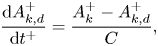 \begin{equation} \frac{{\rm d}A^+_{k,d}}{{\rm d}t^+}=\frac{A_k^+-A^+_{k,d}}{C}, \end{equation}
where  $C=4000$ is a model parameter. A similar approach was explored by Griffin, Fu & Moin (Reference Griffin, Fu and Moin2021), who varied the damping ‘constant’ $A$ as a function of the shape factor. Additionally, Yang et al. (Reference Yang, Sadique, Mittal and Meneveau2015) and Lv et al. (Reference Lv, Huang, Yang and Yang2021) augmented the LoW as follows:
 \begin{equation} U^+ = \frac{1}{\kappa} \ln(y^+)+B+ay/\delta, \end{equation}
and exploited this augmented scaling for near-wall modelling. Here,  $a$ is a constant, and $\delta$ is an outer length scale. The validity of the linear term was recently examined in Monkewitz & Nagib (Reference Monkewitz and Nagib2023), and the data were favourable. The approach in Yang et al. (Reference Yang, Sadique, Mittal and Meneveau2015) was further extended by Hansen et al. (Reference Hansen, Yang and Abkar2023). There, the authors invoked modes from POD analysis to augment the logarithmic LoW. Modifications of the LoWs can also be found in Knopp et al. (Reference Knopp, Buchmann, Schanz, Eisfeld, Cierpka, Hain, Schröder and Kähler2015), Knopp (Reference Knopp2022), Wei et al. (Reference Wei, Li, Knopp and Vinuesa2023) and Wei & Knopp (Reference Wei and Knopp2023), although the efficacy of these modifications in the context of near-wall turbulence modelling are yet to be consolidated. Along the same line, Fowler et al. (Reference Fowler, Zaki and Meneveau2022) proposed Lagrangian relaxation towards equilibrium. The model has a component that accounts for the laminar Stokes layer response in the viscous sublayer to fast-varying pressure gradients. In summary, while the existing models have achieved many successes, the absence of a robust velocity scaling for PG TBLs necessitates the reliance on empiricism, sometimes at the price of many model parameters.
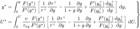
Having fewer parameters is almost always desirable. The objective of this work is to develop a near-wall model without relying on heuristics and empiricism. This requires a velocity scaling valid for flows with arbitrary pressure gradient forces. Such a velocity scaling was recently developed by Chen et al. (Reference Chen, Wu, Griffin, Shi and Yang2023),
 \begin{equation} \left. \begin{aligned}
y^* & =\int_0^y \frac{F(y^*)}{F'(y^*)}\left[
\frac{1}{\tau^+}\frac{\partial \tau^+}{\partial y} -
\frac{1}{1+g}\frac{\partial g}{\partial y} +
\frac{F'(y^+_0)}{F(y^+_0)}\frac{{\rm d} y_0^+}{{\rm d}
y}\right] \,{{\rm d} y},\\ U^* & =\int_0^U
\frac{\nu}{\tau_{xy}} \frac{F(y^*)}{F'(y^*)}\left[
\frac{1}{\tau^+}\frac{\partial \tau^+}{\partial y} -
\frac{1}{1+g}\frac{\partial g}{\partial y} +
\frac{F'(y^+_0)}{F(y^+_0)}\frac{{\rm d} y_0^+}{{\rm d}
y}\right] \,{\rm d}U, \end{aligned} \right\}
\end{equation}
\begin{equation} \left. \begin{aligned}
y^* & =\int_0^y \frac{F(y^*)}{F'(y^*)}\left[
\frac{1}{\tau^+}\frac{\partial \tau^+}{\partial y} -
\frac{1}{1+g}\frac{\partial g}{\partial y} +
\frac{F'(y^+_0)}{F(y^+_0)}\frac{{\rm d} y_0^+}{{\rm d}
y}\right] \,{{\rm d} y},\\ U^* & =\int_0^U
\frac{\nu}{\tau_{xy}} \frac{F(y^*)}{F'(y^*)}\left[
\frac{1}{\tau^+}\frac{\partial \tau^+}{\partial y} -
\frac{1}{1+g}\frac{\partial g}{\partial y} +
\frac{F'(y^+_0)}{F(y^+_0)}\frac{{\rm d} y_0^+}{{\rm d}
y}\right] \,{\rm d}U, \end{aligned} \right\}
\end{equation}
where the transformed velocity  $U^*$ follows the established LoW as a function of $y^*$. Here, $\tau ^+=\tau _{xy}/\tau _{xy,w}$, $F(\phi )=1+\kappa \phi (1-\exp (-\phi /A))^2$ describe the behaviour of the total shear stress in the inner layer of an equilibrium boundary layer; $F'$ is the derivative of $F$, and $g$ is the Lagrangian integration of the total shear stress
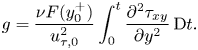 \begin{equation} g=\frac{\nu F(y^+_0)}{u_{\tau,0}^2} \int_0^t\dfrac{\partial^2 \tau_{xy}}{\partial y^2}\,{\rm D}t. \end{equation}
This  $g$ accounts for the history effect. In the absence of any pressure gradient force, the transformation degenerates to the LoW and $y^*=y^+$, $U^*=U^+$. In the presence of a pressure gradient, the transformation provides a description of the mean flow in boundary layers.
With the knowledge of the mean flow scaling, developing a wall model involves inverting the mean flow scaling. This is often straightforward. For example, inverting the LoW in (1.1) leads to the algebraic EWM in (1.2). Yang & Lv (Reference Yang and Lv2018), among others (Chen et al. Reference Chen, Lv, Xu, Shi and Yang2022; Griffin, Fu & Moin Reference Griffin, Fu and Moin2023; Hendrickson et al. Reference Hendrickson, Subbareddy, Candler and Macdonald2023), have inverted velocity and temperature transformations for wall modelling of high-Mach-number boundary-layer flows. However, inverting the velocity transformation in Chen et al. (Reference Chen, Wu, Griffin, Shi and Yang2023) is highly non-trivial. Unlike the existing velocity transformations that rely solely on local information, the velocity transformation in (1.7) requires the integration of the total shear stress, which is non-local and not readily available. Due to the involvement of this non-local information, the transformation in (1.7) was presented as a descriptive tool in Chen et al. (Reference Chen, Wu, Griffin, Shi and Yang2023). A primary objective of this work is to overcome this difficulty and exploit the velocity transformation in (1.7) for predictive modelling. More specifically, we will introduce a new transport equation, through which a new wall-normal coordinate is defined. The use of this wall-normal coordinate in the eddy viscosity formulation gives rise to a new closure for the Reynolds shear stress.
The rest of the paper is organized as follows. We present the flow problem, the governing equation and the modelling objectives in § 2. In § 3, we present the details of our model, along with a summary of four existing inner-layer models. In §§ 4 and 5, we provide specifics about the validation data and the computational set-up. The results are presented in § 6 with further discussion in § 7. Lastly, we conclude in § 8.
2. Flow problem, governing equation and modelling task
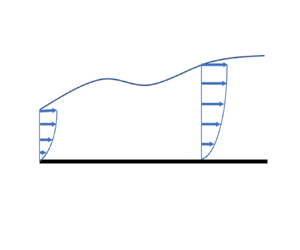
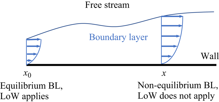
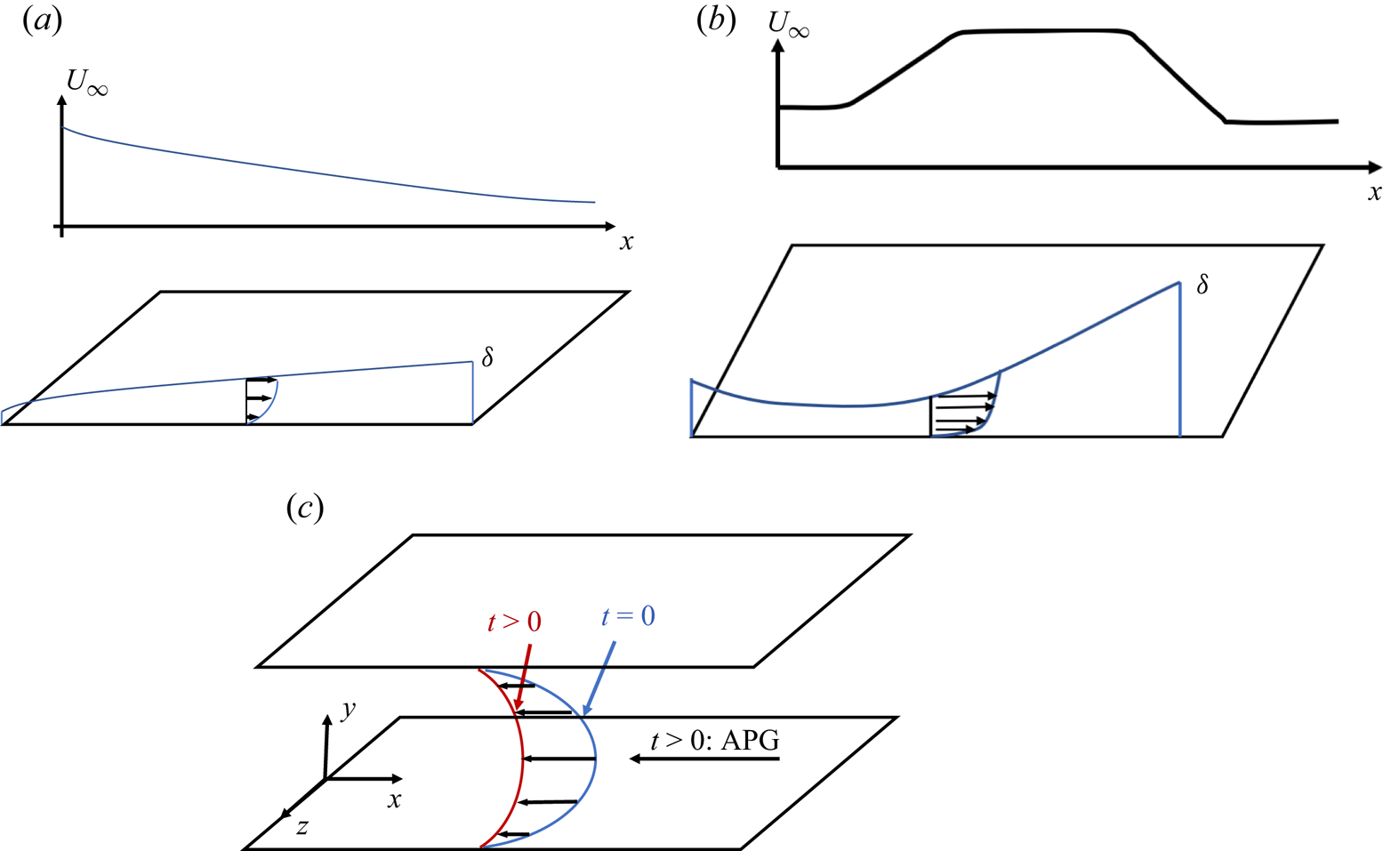
Consider the flow depicted in figure 1. We assume that the mean flow is two-dimensional and remains attached to the wall, i.e. before incipient separation. There is a non-negligible pressure gradient, but the flow is initially a fully developed TBL.
Schematic of the flow problem. The initial equilibrium boundary layer (BL) is subjected to some arbitrary pressure gradients.
The evolution of the mean flow is governed by the following ensemble-averaged continuity and  $x$-momentum equations:
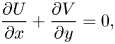 \begin{equation} \frac{\partial U}{\partial x}+\frac{\partial V}{\partial y}=0, \end{equation}
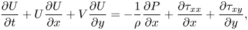 \begin{equation} \frac{\partial U}{\partial t}+U\frac{\partial U}{\partial x}+V\frac{\partial U}{\partial y}={-}\frac{1}{\rho}\frac{\partial P}{\partial x}+\frac{\partial \tau_{xx}}{\partial x}+\frac{\partial \tau_{xy}}{\partial y}, \end{equation}
where
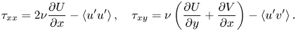 \begin{equation} \tau_{xx}=2\nu\frac{\partial U}{\partial x}-\left\langle u'u'\right\rangle,\quad \tau_{xy}=\nu\left(\frac{\partial U}{\partial y}+\frac{\partial V}{\partial x}\right)-\left\langle u'v'\right\rangle. \end{equation}
Here,  $U$,
$U$,  $V$ and $W$ are the mean velocity in the three Cartesian directions, $u'$,
$u'$,  $v'$ and $w'$ are the velocity fluctuations, $\tau$ is the stress and $\left \langle {\cdot }\right \rangle$ denotes ensemble averaging. Note that the ensemble average allows us to keep the unsteady term without invoking any assumption about the time scales involved in the flow.
Equations in (2.1), (2.2) and (2.3a,b) can be simplified by invoking the thin boundary layer approximation:
 \begin{equation} \frac{\partial V}{\partial x}\ll\frac{\partial U}{\partial y},\quad \frac{\partial \tau_{xx}}{\partial x}\ll\frac{\partial \tau_{xy}}{\partial y}. \end{equation}
It follows that
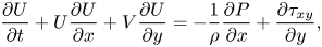 \begin{equation} \frac{\partial U}{\partial t}+U\frac{\partial U}{\partial x}+V\frac{\partial U}{\partial y}={-}\frac{1}{\rho}\frac{\partial P}{\partial x}+\frac{\partial \tau_{xy}}{\partial y}, \end{equation}
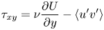 \begin{equation} \tau_{xy}=\nu\frac{\partial U}{\partial y}-\left\langle u'v'\right\rangle \end{equation}
and
 \begin{equation} \frac{\partial P}{\partial y}=0. \end{equation}
 The Reynolds shear stress  $-\left \langle u'v'\right \rangle$ is the only unclosed term in (2.1), (2.5), (2.6) and (2.7). We invoke the eddy viscosity $\nu _t$ and rewrite the Reynolds shear stress term as follows:
 \begin{equation} -\left\langle u'v'\right\rangle=\nu_t\frac{\partial U}{\partial y}. \end{equation}
The modelling objective is to find the eddy viscosity  $\nu _t$.
3. Near-wall models
In addition to a near-wall model based on the velocity transformation in (1.7), which we will elaborate in § 3.2, we will also examine four models in the existing literature: the baseline SA model (Spalart & Allmaras Reference Spalart and Allmaras1992); the Wilcox  $k$–
$k$– $\omega$ model (Wilcox Reference Wilcox1991); the EWM; and the EWM with Kays’ empirical correction (Kays et al. Reference Kays, Crawford and Weigand2004). The comparative study will provide insights into the physics that is missing in the existing models and identify scenarios where the missing physics makes a significant difference.
The SA model and the Wilcox  $k$–
$k$– $\omega$ model involve solving one and two additional transport equations, respectively, alongside the RANS equations to determine the eddy viscosity. These two models are extensively used in fluids engineering practice. Detailed documentation can be found on the Turbulence Modeling Resource website (https://turbmodels.larc.nasa.gov/) and is not repeated here for brevity. The EWM and Kays’ model are mixing-length-type models. We provide a succinct overview of these two models in § 3.1.
3.1. Mixing-length-type models
The mixing-length model has roots tracing back to Prandtl (Reference Prandtl1925). It formulates the eddy viscosity as
 \begin{equation} \nu_t=l^2\frac{\partial U}{\partial y}, \end{equation}
where  $l$ is the mixing length. The mixing length is given by
 \begin{equation} l=\min[l_{IL},l_{OL}], \end{equation}
where  $l_{IL}$ is the inner-layer mixing length and $l_{OL}$ is the outer-layer mixing length. The discussion here focuses on the inner layer $l_{IL}$. For the outer layer, we adopt the value $l_{OL}=0.085 \delta$ as from Kays et al. (Reference Kays, Crawford and Weigand2004), where $\delta$ is the outer length scale, i.e. the half-channel height or the boundary layer thickness.
Several models have been proposed for  $l_{IL}$. The EWM models the $l_{IL}$ as
 \begin{equation} l_{IL}=\kappa y D, \end{equation}
where  $D$ is a damping function, and a common choice is (Van Driest Reference Van Driest1956)
 \begin{equation} D_v=1-\exp({-}y^+{/}A^+_{VD}), \end{equation}
where  $A^+_{VD}=26$. Kays et al. (Reference Kays, Crawford and Weigand2004) retained (3.3), but employed a PG-dependent damping coefficient in (1.4). Note that (1.4) is calibrated for boundary layer flow configuration but is also applicable to channel flow thanks to the universality of the inner layer. Equations (3.1), (3.2), (3.3) and (3.4) constitute the EWM and (3.1), (3.2), (3.3) and (1.4) constitute Kays’ model.
3.2. Present model
We invert the velocity transformation in (1.7) for wall modelling. To do that, we need knowledge of the Lagrangian integration of the total shear stress. To that end, we define
 \begin{equation} \phi\equiv \int_0^t \frac{\partial^2\tau_{xy}}{\partial y^2}\,{\rm D}t. \end{equation}
Taking the material derivative of the two sides of (3.5), we have
 \begin{equation} \frac{{\rm D}\phi}{{\rm D}t}=\frac{\partial^2\tau_{xy}}{\partial y^2}, \end{equation}
where the  $\textrm {D}/\textrm {D}t$ is the material derivative, $\tau _{xy}$ is the total stress and is given by $\tau _{xy}= (\nu +\nu _t)\partial U/\partial y$ according to (2.8). This yields a transport equation governing $\phi$:
 \begin{equation} \frac{{\rm D}\phi}{{\rm D}t}=\frac{\partial^2}{\partial y^2}\left[(\nu+\nu_t)\frac{\partial U}{\partial y}\right]. \end{equation}
Equation (3.7) yields the Lagrangian integration of the total shear stress. When combined with (1.7), the two equations yield a value for  $y^*$. The eddy viscosity $\nu _t^+$ is a universal function of $y^*$ regardless of whether the boundary layer is subjected to a pressure gradient or not (Chen et al. Reference Chen, Wu, Griffin, Shi and Yang2023). Therefore, (3.1), (3.2), (3.3) and (3.4) remain valid, with the only modification being the replacement of $y^+$ in (3.4) with $y^*$:
 \begin{equation} D_s=1-\exp({-}y^*/A^+_{VD}), \end{equation}
where  $A^+_{VD}=26$ and does not change. To summarize, the knowledge of $y^*$ leads to a model for $\nu _t$ and a closure of the Reynolds shear stress, thereby completing the model.
Compared with Kay's augmentation, which is empirical and involves adjustable parameters, the present model involves no additional adjustable parameters (other than those already in the EWM). Besides, the simplicity of this derivation is worth noting.
4. Data
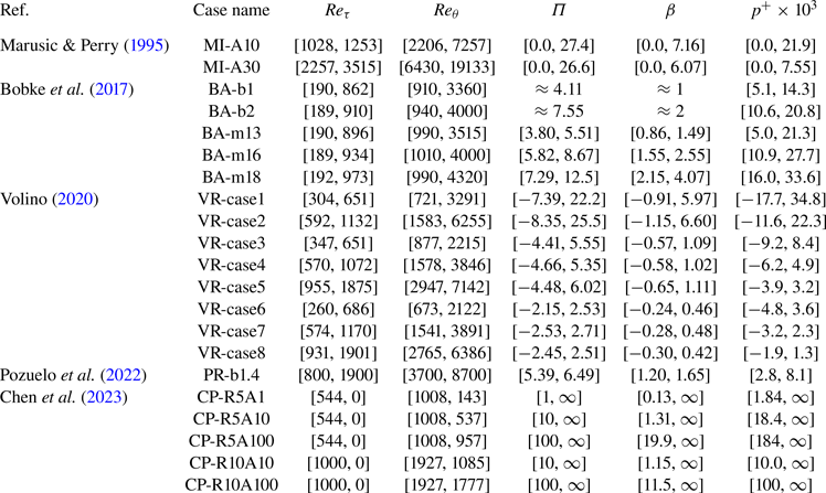
We will rely on the experimental data in Marusic & Perry (Reference Marusic and Perry1995) and Volino (Reference Volino2020) and the computational data in Bobke et al. (Reference Bobke, Vinuesa, Örlü and Schlatter2017), Pozuelo et al. (Reference Pozuelo, Li, Schlatter and Vinuesa2022) and Chen et al. (Reference Chen, Wu, Griffin, Shi and Yang2023) for validation. The data in Marusic & Perry (Reference Marusic and Perry1995), Bobke et al. (Reference Bobke, Vinuesa, Örlü and Schlatter2017), Pozuelo et al. (Reference Pozuelo, Li, Schlatter and Vinuesa2022) and Volino (Reference Volino2020) are boundary-layer data, and the data in Chen et al. (Reference Chen, Wu, Griffin, Shi and Yang2023) are channel-flow data. Figure 2 shows schematics of the flows in these references. Table 1 provides further details, where we list the range of  $Re_\tau =\rho ^{1/2} \tau _w^{1/2} \delta /\mu$, $Re_\theta =\rho U_c \theta /\mu$, $\varPi =({\delta }/{\tau _w})\,\textrm {d}P/{\textrm {d}{\kern0.7pt}x}$, $p^+=\mu /(\rho ^{1/2}\tau _w^{3/2})\,\textrm {d}P/{\textrm {d}{\kern0.7pt}x}$ and $\beta =\delta ^*/\tau _w \,\textrm {d}P/{\textrm {d}{\kern0.7pt}x}$. Here, $U_c$ is the free stream velocity or the velocity at the channel centreline, $\mu$ is the viscosity, $\theta$ is the momentum thickness and $\delta ^*$ is the displacement thickness. Here $p^+$, $\varPi$ and $\beta$ all measure the pressure gradient. Here, we prefer $p^+$ because the inner layer of channel and boundary layer flows are not fundamentally different. The nomenclature of the cases adheres to that used in the original papers with the initials of the leading author placed at the front (see table 1, first two columns). The two MI cases primarily differ in their Reynolds numbers. The five BA cases differ mainly in the pressure gradients and the history of the pressure gradients. The PR case has a similar set-up as BA-m16 with a larger domain and a larger $Re_\theta$. The eight VR cases exhibit differences primarily in their pressure gradients with case1 experiencing the strongest pressure gradient among the eight cases and case8 the weakest. Lastly, the five CP cases differ in Reynolds numbers and pressure gradients. The MI, BA, PR and VR cases and the cases CP-R5A1, CP-R5A10 and CP-R10A10 are subjected to weak to moderate pressure gradients, where a log layer is still discernible. The cases CP-R5A100 and CP-R10A100 are subjected to strong pressure gradients that break the log law. The flows in all but Pozuelo et al. (Reference Pozuelo, Li, Schlatter and Vinuesa2022) are rather typical. The boundary layer flow in Pozuelo et al. (Reference Pozuelo, Li, Schlatter and Vinuesa2022) features an overshoot of the mean velocity near the edge of the boundary layer, and the velocity at $\delta$ is larger than that in the free stream. The non-zero $\partial U/\partial y$ is arguably physical and is due to the irrotational free stream $\partial U/\partial y-\partial V/\partial x=0$ and a non-zero $\partial V/\partial x$ in a PG TBL (Griffin et al. Reference Griffin, Fu and Moin2021). Nonetheless, this effect is only noticeable when the streamwise development length is long and the vertical domain size is large, which is why most of the existing studies, including those referenced here, report a single $U_\infty$ rather than the profile of the velocity in the free stream.
Schematics of the flows in (a) Marusic & Perry (Reference Marusic and Perry1995), Bobke et al. (Reference Bobke, Vinuesa, Örlü and Schlatter2017) and Pozuelo et al. (Reference Pozuelo, Li, Schlatter and Vinuesa2022), (b) Volino (Reference Volino2020) and (c) Chen et al. (Reference Chen, Wu, Griffin, Shi and Yang2023). Here, APG stands for adverse pressure gradient.
Details of the data in Marusic & Perry (Reference Marusic and Perry1995), Bobke et al. (Reference Bobke, Vinuesa, Örlü and Schlatter2017), Pozuelo et al. (Reference Pozuelo, Li, Schlatter and Vinuesa2022), Volino (Reference Volino2020) and Chen et al. (Reference Chen, Wu, Griffin, Shi and Yang2023).
5. Details of the computational set-up
5.1. Boundary-layer cases
We solve the mean flow equations (2.1), (2.5), (2.6) and (2.7) on a two-dimensional grid. Spatial discretization is based on a second-order central finite difference scheme. Pseudo-time-stepping uses the forward Euler scheme. The grids are uniformly spaced in the streamwise direction and stretched in the wall-normal direction. The first off-wall grid is such that  $\Delta y^+_w<1$, and the grid spacing in the outer layer is such that $\Delta x^+<104$ and
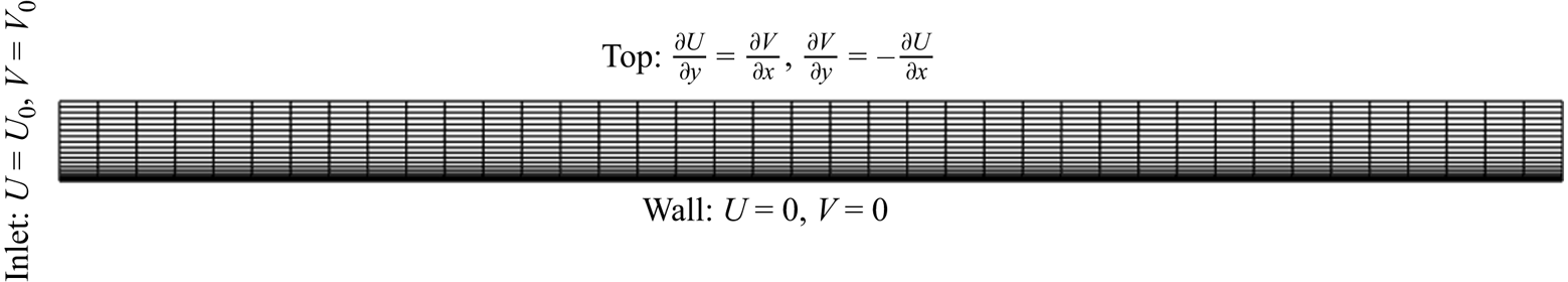
  $\Delta y^+<22$. The adequacy of the grid is validated through a grid convergence study (not shown). Figure 3 is a schematic of the computational domain. The boundary conditions are as follows. Profiles of a fully developed boundary layer are obtained from separate zero-pressure-gradient TBL calculations and placed at the left-hand boundary. The right-hand boundary is a non-reflective outlet. The top boundary is a zero-vorticity one. Lastly, the bottom boundary is a no-slip, no-penetration wall. The domain size is as follows. The streamwise size of the domain matches that in the original references. The vertical size is adjusted such that $L_y/\delta$ matches that in the original paper at the left-hand boundary.
Schematic of the computational domain.
Pressure gradient information is also needed. This information is directly available in Bobke et al. (Reference Bobke, Vinuesa, Örlü and Schlatter2017) and Pozuelo et al. (Reference Pozuelo, Li, Schlatter and Vinuesa2022) but not in Marusic & Perry (Reference Marusic and Perry1995) and Volino (Reference Volino2020). Therefore, we must infer the pressure gradient from the measurements reported in Marusic & Perry (Reference Marusic and Perry1995) and Volino (Reference Volino2020). In Marusic & Perry (Reference Marusic and Perry1995), the free stream velocity was reported. Following Volino (Reference Volino2020) and applying Bernoulli's equation in the free stream gives
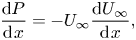 \begin{equation} \frac{{\rm d}P}{{\rm d}{\kern0.7pt}x}={-}U_\infty\frac{{\rm d}U_\infty}{{\rm d}{\kern0.7pt}x} , \end{equation}
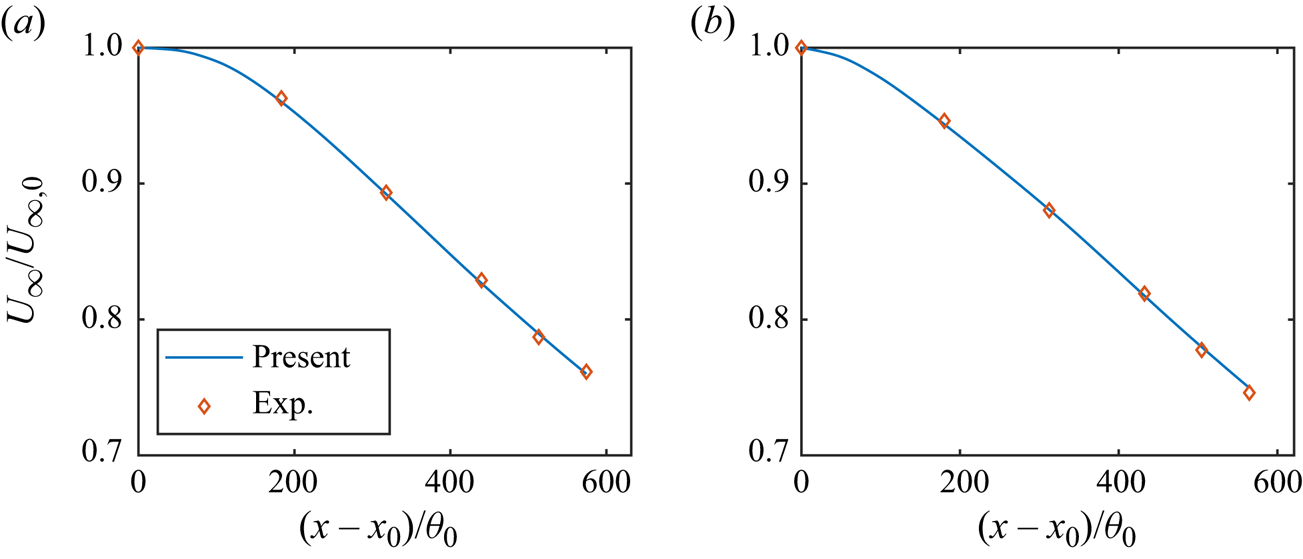
which allows us to obtain the pressure gradient information. Equation (5.1) incurs uncertainty when the vertical domain size is large (Pozuelo et al. Reference Pozuelo, Li, Schlatter and Vinuesa2022) but is sufficient for the cases in Marusic & Perry (Reference Marusic and Perry1995). As a validation of (5.1), figure 4 compares the free stream velocity  $U_\infty (x)$ in our calculations with the values reported in the paper, and there is a good agreement. Volino (Reference Volino2020) reported the parameter
 \begin{equation} K=\frac{\nu}{U_\infty^2} \frac{{\rm d}U_\infty}{{\rm d}{\kern0.7pt}x}, \end{equation}
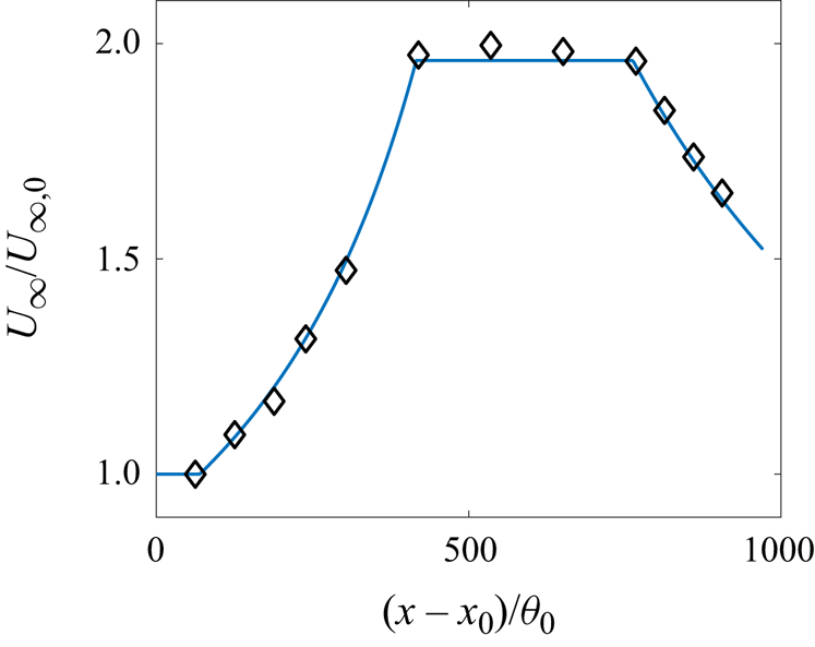
from which we can compute the pressure gradient. Figure 5 compares the resulting free stream velocity  $U_\infty (x)$ in our calculation with the ones reported in Volino (Reference Volino2020) for the VR-case1 – there is also a good agreement. The results in the other VR cases are similar and are not reported here for brevity.
The free stream velocity in (a) MI-A10 and (b) MI-A30. The symbols are experimental data reported in Marusic & Perry (Reference Marusic and Perry1995), and the lines are results from the present calculations.
The free stream velocity in VR-case1. The symbols are experimental data reported in Volino (Reference Volino2020) and the line is from our calculation.
5.2. Channel flow case
The set-up of the channel flow cases is similar to that of the boundary layer cases except that the flow is one-dimensional in space and evolves in time. The initial condition corresponds to a fully developed channel and is obtained from a separate plane channel calculation. The pressure gradient information is readily available in Chen et al. (Reference Chen, Wu, Griffin, Shi and Yang2023).
6. Results
We compare the model results with the data from the literature, focusing primarily on the evolution of skin friction.
6.1. Boundary layer
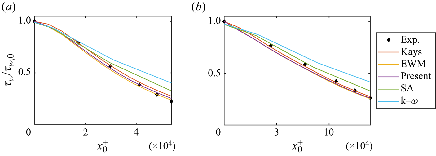
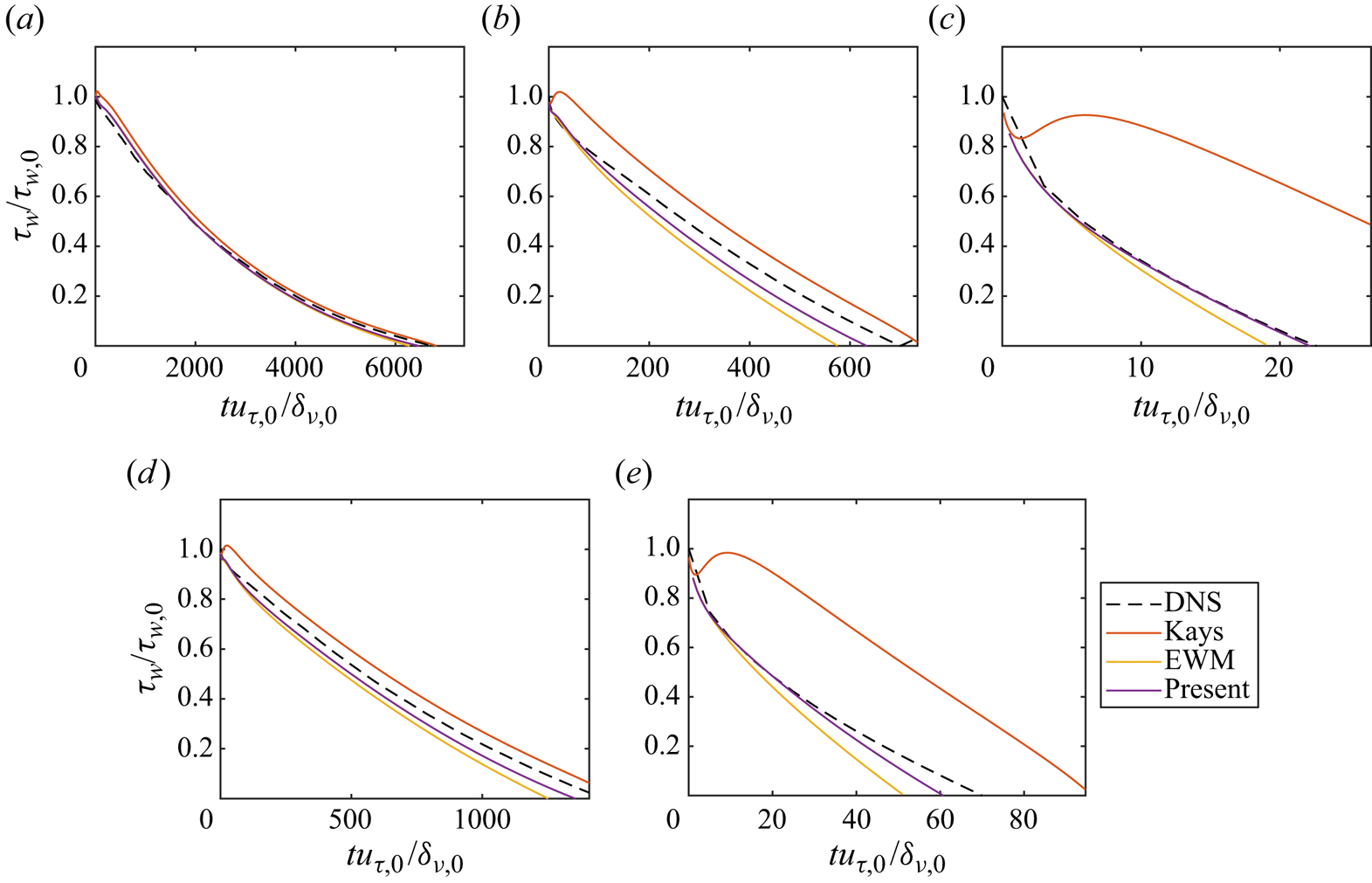
Figure 6 displays the wall-shear stress results for the MI cases, and figure 7 presents the results for the BA cases. Both the two RANS models significantly over-predict the wall-shear stress with the SA model providing slightly more accurate results than the Wilcox  $k$–
$k$– $\omega$ model for the MI cases and the Wilcox $k$–
$k$– $\omega$ model providing slightly more accurate results than the SA model for the BA cases. For both the two MI cases, the EWM, Kays’ model and the present velocity-transformation-based model yield nearly identical results. For BA cases, Kays’ model emerges as the most accurate, with the present model and the EWM slightly under-predicting the wall-shear stress. Given the less-than-ideal performance of the two RANS models, subsequent discussions will primarily focus on the two mixing length models and the present velocity-transformation-based model.
Wall-shear stress in (a) MI-A10 and (b) MI-A30. Here, normalization is relative to inlet values at  $x=0$. The reference experimental data are from Marusic & Perry (Reference Marusic and Perry1995).
Wall-shear stress in (a) BA-b1, (b) BA-b2, (c) BA-m13, (d) BA-m16 and (e) BA-m18. The reference LES data are from Bobke et al. (Reference Bobke, Vinuesa, Örlü and Schlatter2017).
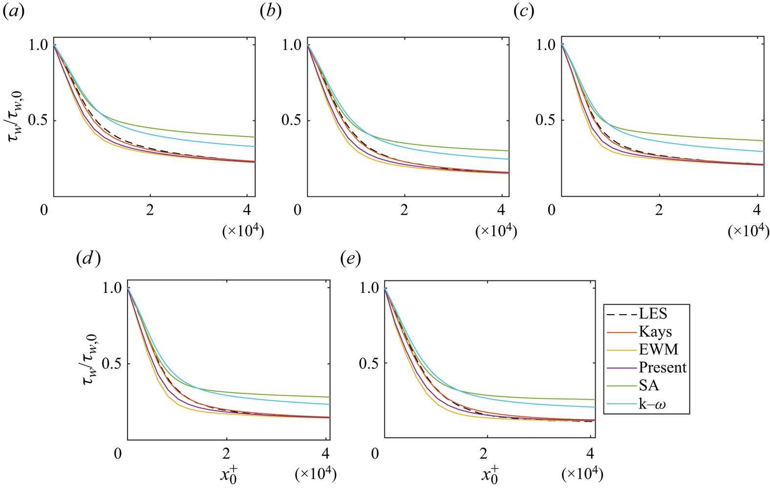
Figure 8 presents the wall-shear stress for VR cases. For VR-case4 to case8, where the pressure gradients are weak, all models yield essentially identical results. For case1 to case3, Kays’ model closely follows the reference data. The EWM and the present model slightly over-predict the wall-shear stress in the favourable pressure gradient regions and slightly under-predict the wall-shear stress in the adverse pressure gradient regions.
The wall shear stress from (a) VR-case1, (b) VR-case2, (c) VR-case3, (d) VR-case4, (e) VR-case5, (f) VR-case6, (g) VR-case7 and (h) VR-case8. Experiment data are from Volino (Reference Volino2020).
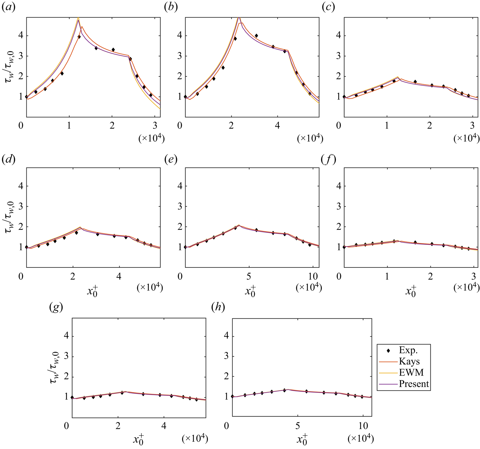
The results for the PR case are shown in figure 9(a). The results are similar to the other boundary-layer cases, and all models perform well. Recall that the pressure gradient information is directly available from the reference, but if this information was not available, one would need to infer that from the free stream velocity, which varies as a function of the distance from the wall above the edge of the boundary layer. Here, we study how the choice of  $U_\infty$ affects the results. Figure 9(b) depicts the pressure gradient when we set $U_\infty$ to the edge velocity $U_e$ or the velocity at the top of the computational domain $U_{top}$. (Here, the edge velocity $U_e$ is computed from the diagnostic plot method (Vinuesa et al. Reference Vinuesa, Bobke, Örlü and Schlatter2016).) The resulting wall-shear stresses are shown in figure 9(a), and we see the choice of $U_\infty$ has a significant impact on the wall-shear stress results. Specifically, taking $U_\infty =U_{top}$ leads to under-predictions of the wall-shear stress, whereas taking $U_\infty =U_e$ leads to accurate predictions.
(a) The wall shear stress results in case PR-b1.4. The dashed lines result from taking  $U_\infty =U_{top}$, the dash-dotted lines result from taking $U_\infty =U_e$ and the solid lines result from directly taking the pressure gradient information from Pozuelo et al. (Reference Pozuelo, Li, Schlatter and Vinuesa2022). Note that the solid lines and the dash-dotted lines collapse. (b) The pressure gradient calculated from (5.1). Here $P_{x,r}$ is the pressure gradient reported in Pozuelo et al. (Reference Pozuelo, Li, Schlatter and Vinuesa2022); $P_{x,t}$ is the pressure gradient force when we take $U_\infty =U_{top}$; and $P_{x,e}$ is the pressure gradient force when we take $U_\infty =U_e$. Note that the $P_{x,e}$ and $P_{x,r}$ lines collapse.
We summarize the results in this subsection. While the two RANS models prove to be inaccurate, the two mixing length models and the present velocity-transformation-based model provide accurate wall-shear stress estimates for the boundary layer cases in Marusic & Perry (Reference Marusic and Perry1995), Bobke et al. (Reference Bobke, Vinuesa, Örlü and Schlatter2017), Volino (Reference Volino2020) and Pozuelo et al. (Reference Pozuelo, Li, Schlatter and Vinuesa2022), where the flows are subjected to weak to moderate pressure gradients.
6.2. Channel
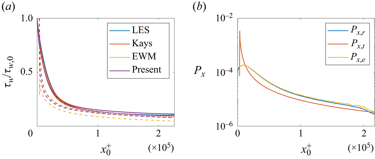
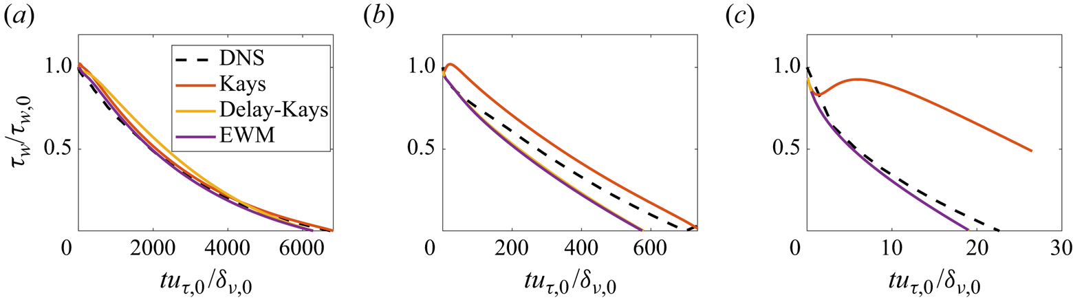
Figure 10 shows the wall-shear stress for the CP cases. When there is a weak pressure gradient, i.e. case R5A1 and figure 10(a), the two mixing length models and the present velocity-transformation-based model all give accurate estimates of the wall-shear stress. For moderate pressure gradients, i.e. cases R5A10 and R10A10 illustrated in figure 10(b,d), Kays’ model slightly overestimates the wall-shear stress, while the EWM and the present velocity-transformation-based model slightly underestimates with the present model being slightly more accurate than the EWM. We also see that Kays’ model predicts an overshoot of the wall-shear stress near  $t=0$. This unphysical behaviour is due to the assumed immediate response of turbulence to the imposed pressure gradient. Nonetheless, in cases R5A10 and R10A10, this is but a minor issue. Lastly, figure 10(c,e) show the results for cases R5A100 and R10A100, which involve strong pressure gradients. In these instances, Kays’ model demonstrates an immediate response to the imposed pressure gradient, resulting in a gross overshoot in the predicted wall-shear stress. On the other hand, the EWM and the present model underestimate the wall-shear stress with the present model being more accurate.
The wall shear stress from (a) CP-R5A1, (b) CP-R5A10, (c) CP-R5A100, (d) CP-R10A10 and (e) CP-R10A100. The direct numerical simulation (DNS) data are from Chen et al. (Reference Chen, Wu, Griffin, Shi and Yang2023).
In many engineering applications, one would be interested in incipient separation. Table 2 lists the time it takes to reach incipient separation. These values offer an additional metric for assessing the models’ accuracy. Upon close examination, it is evident that Kays’ model tends to overestimate the time required for incipient separation, particularly in the presence of strong pressure gradients. In contrast, the EWM consistently underestimates the time it takes for incipient separation. The present velocity-transformation-based model also underestimates this time, but the error it incurs is notably smaller than the EWM.
The time of incipient separation in  $\delta _{\nu,0}/u_{\tau,0}$. The errors in the models are also listed.
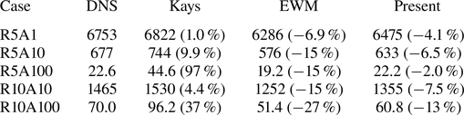
In summary, Kays’ model demonstrates high accuracy under moderate pressure gradients, i.e. within calibration conditions, but incurs significant error in the presence of strong pressure gradients, i.e. outside calibration conditions. The EWM offers satisfactory performance, especially considering its simplicity. The present model, on the other hand, proves to be highly robust, consistently delivering accurate results regardless of the imposed pressure gradient force.
7. Further discussion
7.1. On the flow quantities
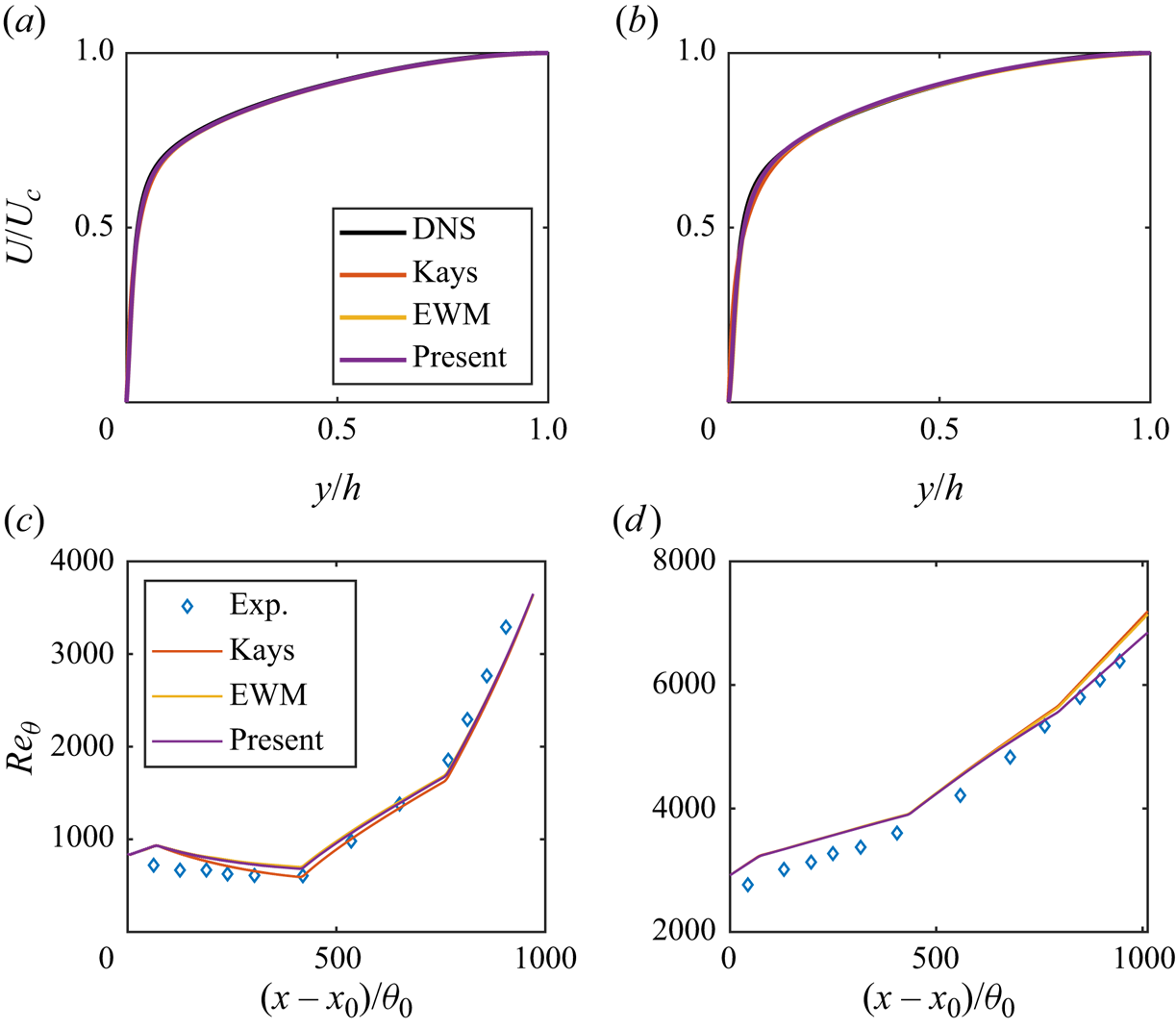
Our discussion focuses on the wall-shear stress. This is because wall-shear stress is more relevant to near-wall turbulence modelling than outer-layer quantities (Hansen et al. Reference Hansen, Yang and Abkar2023). To make this clear, we examine a few outer-layer quantities. Figure 11(a,b) depict the velocity profiles in outer scales for case CP-R5A100 at times  $t_0^+=3$ and 14. This case is where the EWM, Kays’ model and the present velocity-transformation-based model exhibit the most difference. However, we observe minimal disparity in the velocity profiles in figure 11(a,b). Figure 11(c,d) illustrates the momentum thickness in VR-case1 and VR-case8. Once again, we find no discernible distinction between the three models. These results suggest that outer quantities do not provide good measures for the wall models.
Velocity profiles in outer scale in case CP-R5A100 at time (a)  $t_0^+=3$ and (b) $t_0^+=14$. Momentum thickness in (c) VR-case1 and (d) VR-case8.
7.2. Further discussions on Kays’ model
The results in § 6 favour Kays’ model for weak to moderately high pressure gradients, e.g. in the BA cases. We attribute the good results to the calibration in Kays et al. (Reference Kays, Crawford and Weigand2004) rather than the superiority of the model's formulation. To clarify, we invoke a slightly different calibration of the outer layer, i.e. the calibration in Clauser (Reference Clauser1956) and Pirozzoli (Reference Pirozzoli2014),
 \begin{equation} \nu_t=\nu_{to}=C_\mu u_\tau \delta,\quad \text{if }y>\eta^* \delta, \end{equation}
where  $C_\mu =0.0902$, $\delta =1.6\delta _{95}$ is an outer length scale, $\delta _{95}$ measures the height where the mean velocity is 95 % of the edge velocity $U_e$ and $\eta ^*=0.155$. Figure 12 shows the results, where we apply the outer-layer calibration in (7.1) together with the three inner-layer models. The differences between Kays’ model, EWM, and the present model remain small, but this calibration favours our model instead.
Wall shear stress in (a) BA-b2, (b) BA-m13 and (c) BA-m16. Here, the eddy viscosity in the outer layer is modelled according to (7.1).
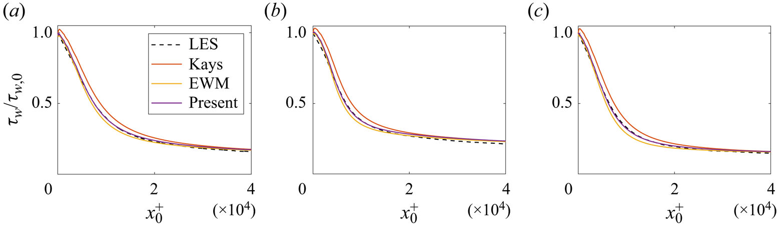
Besides, the results in § 6.2 show that Kays’ model does not perform well when there is a high pressure gradient. This issue is due to the immediate response of the modelled eddy viscosity to the imposed pressure gradient. Kays et al. (Reference Kays, Crawford and Weigand2004) acknowledged the issue, and proposed a correction in (1.5) that delays the model's response. Figure 13 compares the delayed Kays’ model with EWM and the present model for cases R5A1, R5A10 and R5A100. The delayed Kays’ model is slightly less accurate than the baseline Kays’ model in R5A1, where the flow is subjected to a weak pressure gradient force. On the other hand, in R5A10 and R5A100, where there is a moderately high and high pressure gradient force, the delayed Kays’ model is more accurate than its baseline counterpart but still not more accurate than the EWM. The results in other cases, i.e. R10A10 and R10A100, are similar and are not shown here for brevity. Considering that EWM is simpler and contains fewer parameters, one might prefer the EWM in engineering practice.
Wall shear stress in (a) R5A1, (b) R5A10 and (c) R5A100. Here, delay-Kays refers to Kays’ model with the correction in (1.5).
7.3. Accounting for history effects
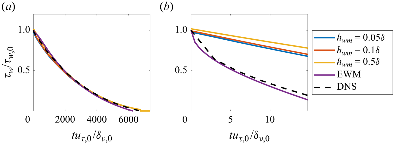
Examining the results in § 6, an interesting observation is that the EWM provides reasonably good wall-shear stress predictions even for moderately high and high pressure gradient TBLs. This may appear counterintuitive since the LoW is a poor approximation of the mean flow in a PG TBL. Indeed, computing the wall-shear stress directly from an off-wall velocity according to the LoW incurs significant errors as we can see from figure 14. There, the wall-shear stress is computed as follows:
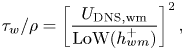 \begin{equation} \tau_w/\rho=\left[\frac{U_{{\rm DNS}, {\rm wm}}}{{\rm LoW}(h_{wm}^+)}\right]^2, \end{equation}
where  $U_{\textrm {DNS},\textrm {wm}}$ is the DNS velocity at the distance $h_{wm}$ from the wall, and the LoW contains both the viscous layer and the logarithmic layer with (7.2) degenerating to (1.2) in the log layer. An interesting question is why the algebraic model in (7.2) performs so poorly yet the EWM, which is also rooted in the LoW, performs reasonably well.
Wall shear stress computed from an off-wall location according to the LoW: (a) R5A1; (b) R5A100. Here  $h_{wm}$ measures the distance from the off-wall location to the wall.
In order to answer this question, we must examine the equations. The algebraic model in (7.2) is a direct consequence of the constant stress layer, namely
 \begin{equation} {-}\frac{\partial \left\langle u'v'\right\rangle}{\partial y}+\nu\frac{\partial^2 U}{\partial y^2}=0. \end{equation}
In other words, (7.2) is a solution to (7.3). The EWM in this paper, on the other hand, corresponds to (2.5). Comparing (7.3) and (2.5), the two equations differ in that (2.5) contains the pressure gradient term  $\textrm {d}P/{\textrm {d}{\kern0.7pt}x}$ and the material time derivative term $\textrm {d}U/\textrm {d}t$. This comparison compels us to conclude that much of the new physics in unsteady wall-bounded turbulence with strong pressure gradients is captured by the material time derivative of mean streamwise momentum and the pressure gradient term, neither of which requires any modelling. Furthermore, by comparing the results of the present velocity-transformation-based model that properly accounts for history effects in PG TBLs and the EWM which neglects history effects in its turbulence closure, we conclude that history effects are important to turbulence modelling only at extreme pressure gradient conditions. Lastly, by comparing Kays’ model and the EWM, we may also conclude that empirical corrections that aim to account for history effects might adversely affect a model's robustness, yielding grossly inaccurate results at extreme pressure gradient conditions.
8. Conclusions
This work develops an inner-layer model for boundary-layer flows subjected to arbitrary pressure gradients. The model is based on the velocity transformation in Chen et al. (Reference Chen, Wu, Griffin, Shi and Yang2023). It entails an additional transport equation that tracks the Lagrangian integration of the total shear stress, a piece of information needed for the velocity transformation. The resulting model is fully predictive yet introduces no new model parameters other than the ones in the EWM. We compare our model with the EWM, Kays’ model, and two RANS models, SA and Wilcox  $k$–
$k$– $\omega$, for a wide range of flows in the literature. For the flows considered in this study, the two RANS models prove to be quite inaccurate. The EWM, Kays’ model and the present velocity-transformation-based model yield very similar results when there are weak, moderate and moderately high pressure gradients, with Kays’ model being slightly more accurate than the present model and the present model being slightly more accurate than the EWM. However, when there is a strong pressure gradient, Kays’ model becomes grossly inaccurate, whereas the present model remains accurate.
In addition to validating a new near-wall model, the comparative study here provides new insights into the boundary-layer flow physics. First, comparing the algebraic wall model in (7.2) and the EWM, we conclude that much of the new physics in PG TBLs is contained in the material time derivative term and the pressure gradient term, both of which require no modelling. Second, comparing the EWM and the present model, we conclude that history effects do not significantly impact the validity of the mixing length model except when there is an extremely high pressure gradient. Third, comparing the EWM and Kays’ models, we conclude that empirical corrections that account for history effects might compromise an otherwise robust model, yielding unphysical results outside the calibration conditions.
We stress that the current conclusions are derived from the test cases of PG TBLs discussed above. While a wide range of PG TBLs are considered, many other types of PG TBLs are left out, e.g. TBLs recovering from a strong adverse pressure gradient followed by a favourable pressure gradient, where the mean flow recovery is slowed down by the even slower turbulence recovery. In these flows, the turbulent stress would play a significant role, and it is not clear if the EWM would still perform well. This calls for additional validation and verification, which we leave for future investigation.
Funding
X.I.A.Y. acknowledges the 2022 CTR summer program. X.I.A.Y. and R.K. acknowledge Office of Naval Research, grant number N000142012315. P.E.S.C. acknowledges the National Natural Science Foundation of grant nos. 12225204 and 11988102. W.Z. acknowledges the support of NSFC (grant no. 12102168).
Declaration of interests
The authors report no conflict of interest.
Data availability statement
The data that support the findings of this study are available from the corresponding author upon reasonable request.


 Open access