




1. Introduction
The dynamics of anisotropic particles in turbulent flows is of crucial importance for a number of industrial and environmental applications (Voth & Soldati Reference Voth and Soldati2017; Hu et al. Reference Hu, Wang, Jia, Zhong and Zhang2021). These particles interact with turbulence in a complex fashion and predicting their behaviour is a long-standing problem, which has been tackled both experimentally and numerically. Numerical investigations have greatly helped to understand the effect of shape on the dynamics, orientation and alignment of anisotropic particles in turbulence. Many works have been focused on homogeneous and isotropic turbulence (HIT), but important works also investigated the influence of non-homogeneity on the particles dynamics in the presence of more complex flows, such as wall-bounded flows (Marchioli, Fantoni & Soldati Reference Marchioli, Fantoni and Soldati2010; Zhao et al. Reference Zhao, Challabotla, Andersson and Variano2015; Zhao & Andersson Reference Zhao and Andersson2016; Cui et al. Reference Cui, Dubey, Zhao and Mehlig2020). Experiments have contributed to a detailed understanding of the dynamics of anisotropic particles, with most of the works in the HIT configuration (Parsa et al. Reference Parsa, Calzavarini, Toschi and Voth2012; Parsa & Voth Reference Parsa and Voth2014; Pujara et al. Reference Pujara, Oehmke, Bordoloi and Variano2018) and only few in turbulent channel flow. In this configuration, recent works by Capone, Miozzi & Romano (Reference Capone, Miozzi and Romano2017) and Shaik et al. (Reference Shaik, Kuperman, Rinsky and van Hout2020) provided velocity and rotation rates of anisotropic particles. These investigations considered long and straight rods, which represent only one of the possible shapes observed in practical applications, where non-axisymmetric particles are frequent. In this work, we focus on a more general class of shapes, represented by slender and non-axisymmetric fibres, i.e. curved fibres in which the length is much larger than the diameter. This geometry has been numerically investigated in the instance of rigid fibres in shear flow (Wang et al. Reference Wang, Abbas, Yu, Pedrono and Climent2018; Thorp & Lister Reference Thorp and Lister2019) and flexible fibres in turbulent channel flow (Dotto & Marchioli Reference Dotto and Marchioli2019; Dotto, Soldati & Marchioli Reference Dotto, Soldati and Marchioli2020). To date, only one experimental work (Alipour et al. Reference Alipour, De Paoli, Ghaemi and Soldati2021) is available in literature and it describes the effect of curvature on the orientation and rotation rate of rigid and curved fibres. However, the effect of the relative size of the fibres to the flow structures has not yet been considered. In this work, we aim precisely at this gap and we investigate experimentally the dynamics of slender, rigid and non-axisymmetric fibres in turbulent channel flow. We focus on the importance of the fibre size relative to the flow scales. This we obtain by maintaining the size of the fibres and increasing the shear Reynolds number. In addition, we chose this fibre size so that fibres remain small compared with the channel height ( $O(10^{-2})$) and the Kolmogorov length scale for all Reynolds number considered.
The wall-normal concentration of straight rods in a channel flow has been investigated in previous works (Krochak, Olson & Martinez Reference Krochak, Olson and Martinez2010; Zhu, Yu & Shao Reference Zhu, Yu and Shao2018) and it was shown to be influenced by both near-wall coherent structures and the fibre aspect ratio. Abbasi Hoseini, Lundell & Andersson (Reference Abbasi Hoseini, Lundell and Andersson2015) observed that fibre–wall interactions depend on fibre size and aspect ratio. The wall-normal fibre distribution is representative of the collective fibre behaviour, but it is not sufficient to investigate in detail the individual fibre dynamics, which is strongly influenced by the fibre velocity. Indeed, the analysis of the mean velocity profile reveals that fibres move faster than the fluid near the wall, possibly suggesting a fibre accumulation in near-wall high-speed regions of the flow (Capone et al. Reference Capone, Miozzi and Romano2017), i.e. in high-speed streaks. In addition to their influence on the wall-normal fibre concentration, the flow structures play a role in the fibre alignment. In the frame of HIT, Ni, Ouellette & Voth (Reference Ni, Ouellette and Voth2014) used the Cauchy–Green strain tensor, which quantifies the Lagrangian stretching experienced by a material element, to analyse the orientation of non-inertial rods and fluid vorticity. They observed that both the fluid vorticity vector and the principal axis of the rods align with the extensional direction of the left Cauchy–Green strain tensor ( $\hat {\boldsymbol {e}}_1$). In this frame, $\hat {\boldsymbol {e}}_1$ is the eigenvector associated with the maximum eigenvalue of the left Cauchy–Green strain tensor, and corresponds to the direction of stretching. The eigenvector $\hat {\boldsymbol {e}}_3$ is associated with the minimum eigenvalue and corresponds to a compression of the fluid element. Finally, the eigenvector $\hat {\boldsymbol {e}}_2$, associated with the intermediate eigenvalue, could correspond to either stretching or compression. It has been observed from the Eulerian strain tensor (Ashurst et al. Reference Ashurst, Kerstein, Kerr and Gibson1987; Huang Reference Huang1996) that, instantaneously, the vorticity tends to align with $\hat {\boldsymbol {e}}_2$. However, Ni et al. (Reference Ni, Ouellette and Voth2014) and Pujara, Voth & Variano (Reference Pujara, Voth and Variano2019) showed that, in HIT, when a Lagrangian measurement is performed, vorticity tends to align with $\hat {\boldsymbol {e}}_1$, as well as non-inertial fibres, provided that the measurements cover a sufficiently long time interval. In the instance of wall-bounded flows, Zhao & Andersson (Reference Zhao and Andersson2016) observed that in the centre of channel and for Lagrangian measurements performed over sufficiently long time intervals, in agreement with what is observed in HIT (Ni et al. Reference Ni, Ouellette and Voth2014), both vorticity and rods align with $\hat {\boldsymbol {e}}_1$. In contrast, in the near-wall region the vorticity preferentially aligns with $\hat {\boldsymbol {e}}_2$, whereas rods align with $\hat {\boldsymbol {e}}_1$. In addition to these results on the alignment of rods, direct numerical simulations of particle-laden flows confirm experimental findings and shed new light on the preferential alignment of spheroids (Voth Reference Voth2015; Zhao et al. Reference Zhao, Challabotla, Andersson and Variano2015). However, the behaviour of curved rigid fibres has not been completely characterised, and it has been proposed that the near-wall fibre dynamics is controlled by sweep and ejection events (Abbasi Hoseini et al. Reference Abbasi Hoseini, Lundell and Andersson2015). Using a three-dimensional reconstruction method, we will provide evidence that supports these findings, and correlate the preferential fibre orientation with the presence of near-wall coherent structures. We also observe that the asymmetry in the fibre shape (curvature) plays a major role in determining the fibre dynamics, and the influence of the flow structures is relevant for fibres with low curvature and in low-speed regions of the flow. We provide a physical explanation to justify the behaviour of the fibres in the near-wall region, and analyse in detail the effect of Reynolds number and fibre shape on fibre concentration, orientation and tumbling. Finally, we will show that, in the limit of straight fibres, our measurements agree with previous experimental and numerical works (Zhao et al. Reference Zhao, Challabotla, Andersson and Variano2015; Shaik et al. Reference Shaik, Kuperman, Rinsky and van Hout2020).
We analysed the behaviour of slender, neutrally buoyant, non-axisymmetric fibres in turbulent channel flow. Experiments are performed in the TU Wien Turbulent Water Channel (Alipour et al. Reference Alipour, De Paoli, Ghaemi and Soldati2021), a 10 m long and 80 cm wide closed water channel (aspect ratio 10) with full optical access. The facility, specifically designed to investigate the behaviour of fibre-laden flows, has been operated for three different values of shear Reynolds number  $ {\textit {Re}}_\tau$, namely $180$, $360$ and $720$. High-speed and time-resolved recordings are used to track the fibres. Finally, a tomographic reconstruction (Elsinga et al. Reference Elsinga, Scarano, Wieneke and van Oudheusden2006) coupled with a discrimination and modelling algorithm (Alipour et al. Reference Alipour, De Paoli, Ghaemi and Soldati2021) is used to identify the fibre shape and orientation. Fibres are divided in three different classes, according to their mean value of curvature (i.e. to their shape). The results are presented in terms of wall-normal fibre concentration, orientation, velocity and tumbling rates for all Reynolds numbers and curvatures considered.
The paper is organised as follows: in § 2, the experimental facility and the methodology are described. Results are presented in terms of the wall-normal distribution of fibre concentration, velocity, orientation and tumbling in § 3, and the effect of the turbulent coherent structures is analysed. Results are also compared with previous numerical and experimental measurements. Finally, in § 4 we provide an overview of the results obtained and of the interplay of fibre dynamics and near-wall flow structures.
2. Experimental set-up
In this work, we performed three-dimensional tracking of fibres in turbulent channel flow. The fibres are polyamide based, slender and non-axisymmetric. A microscope view in dry conditions is reported in figure 1(a). We use the experimental facility, fibre modelling and tracking methodology presented in Alipour et al. (Reference Alipour, De Paoli, Ghaemi and Soldati2021). Measurements are performed at three different values of shear Reynolds number, namely  $ {\textit {Re}}_{\tau }=180$, 360 and 720. The shear Reynolds number, $ {\textit {Re}}_\tau =u_\tau h/\nu$, is based on shear velocity ( $u_\tau$), half-channel height ( $h=40$ mm) and kinematic viscosity of the fluid ( $\nu$). The shear velocity is obtained by fitting the mean streamwise velocity profile obtained experimentally to the velocity profile obtained from direct numerical simulations (Moser, Kim & Mansour Reference Moser, Kim and Mansour1999; Alipour et al. Reference Alipour, De Paoli, Ghaemi and Soldati2021; Iwamoto, Suzuki & Kasagi Reference Iwamoto, Suzuki and Kasagi2002). In the following, we briefly report on the experimental apparatus (channel geometry, imaging system and fibre properties, § 2.1), on the single-phase flow statistics (§ 2.2) and on the fibre discrimination, modelling and tracking approach (§ 2.3).
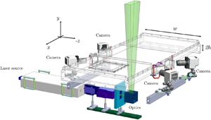
(a) Sample of fibres used for the experiments. Fibres are polyamide based and appear as slender and non-axisymmetric objects. Fibre shapes are classified according to their mean curvature,  $\kappa ^{*}$. Three fibres, corresponding to the three different curvature classes used throughout this work, are highlighted in red. (b) Test section of the TU Wien Turbulent Water Channel. Dimensions of the cross-section, width $w$ and height $2h$, are indicated. The laser volume, represented by the green region and obtained through a series of optics located below the channel, is placed at the channel mid-span. Four cameras looking through water-filled prisms are used to record the three-dimensional motion of the particles. To reduce the optical image distortion due to astigmatism, cameras look through prisms filled with water. The laboratory reference frame ( $x,y,z$, respectively streamwise, wall-normal and spanwise directions) is also shown.

2.1. Experimental apparatus and fibre properties
The experiments are performed in the TU Wien Turbulent Water Channel, a 10 m long closed channel with a cross-section of  $80\ {\rm cm}\times 8\ {\rm cm}$ ( $w\times 2h$, where $h$ is the half-channel height). The flow is driven by gravity and the test section (shown in figure 1b) is located approximately 8.5 m downstream from the entrance. The fluid used for the experiments is water at the average temperature of $15\,^{\circ }{\rm C}$, for which the kinematic viscosity is $\nu =1.1386\times 10^{-6}\ {\rm m}^{2}\ {\rm s}^{-1}$ (Huber et al. Reference Huber, Perkins, Laesecke, Friend, Sengers, Assael, Metaxa, Vogel, Mare and Miyagawa2009).
The imaging system consists of a high-speed laser (527 nm, double cavity, 25 mJ per pulse, pulse repetition 1–50 kHz Litron LD60-532 PIV) and four Phantom VEO 340 L cameras (sensor size of  $2560\times 1600$ pixel at 0.8 kHz). The cameras, located in linear configuration at the sides of the channel as in figure 1(b), are equipped with Scheimpflug adaptors and look through water-filled prisms to minimise the optical astigmatism. The measurement volume, located at the mid-span of the channel, has a size that is changed with the Reynolds number. Details of flow and imaging parameters for all experiments considered are reported in table 1. Image acquisition and single-phase velocimetry have been carried out using Davis 10 (LaVision GmbH).
Summary of the flow and imaging parameters adopted. The reference and effective Reynolds numbers, respectively  $ {\textit {Re}}_{\tau }$ and $ {\textit {Re}}_{\tau,{eff}}$, are reported. Imaging parameters for the single-phase (water) and particle-laden (fibres) are indicated. The time interval $\Delta t$ over which statistics are collected is also indicated. In single-phase recordings, ‘ $^{*}$’ refers to the full recording time. Statistics are ensemble averaged over uncorrelated fields equally spaced in time (1 s for all $ {\textit {Re}}_\tau$). For instance, for $ {\textit {Re}}_\tau =720$, 1920 uncorrelated velocity fields are used to compute the mean velocity profile. Viscous time scale ( $\tau =\nu /u^{2}_\tau$) and length scale ( $\nu /u_\tau$), as well as dimensionless fibre length scale ( $L_{f}^{+}=L_{f}u_\tau /\nu$) are indicated for all $ {\textit {Re}}_\tau$ considered.

To investigate the behaviour of non-axisymmetric objects, we used polyamide 6.6 (PA6.6) precision cut flock (Flockan) fibres. The fibres, a sample of which in dry conditions is reported in figure 1(a), have density  $\rho =1.15\times 10^{3}\ {\rm kg}\ {\rm m}^{-3}$ and cutting length $L_{f}=1.2$ mm (linear density of 0.9 dtex, diameter $d_{f}\approx 10\ \mathrm {\mu }\text {m}$). Fibres, which appear as planar and slender objects (anisotropy ratio, $\lambda =L_{f}/d_{f}\approx 120$), are characterised by a curvature that is also visible to the naked eye. Using the Euler–Bernoulli theory for beams, given the fibre Young's modulus (Bunsell Reference Bunsell2001) and the drag coefficient of the rods (Tang et al. Reference Tang, Tian, Yan and Yuan2014), we estimated that fibre deformation due to flow conditions is reasonably small (less than 1 % of the fibre length for straight fibres, and even lower in the instance of curved ones). Therefore, we will consider the fibres to be rigid objects. Fibres with a smaller Young's modulus can, however, exhibit large deformations and very different interactions with the flow (Allende, Henry & Bec Reference Allende, Henry and Bec2018), and the present findings might not apply. The Stokes number of the fibres (Bernstein & Shapiro Reference Bernstein and Shapiro1994; Alipour et al. Reference Alipour, De Paoli, Ghaemi and Soldati2021), calculated as the ratio of fibre response time to the viscous time of the flow ( $\tau =\nu /u^{2}_\tau$) varies between $ {\textit {St}}=0.001$ ( $ {\textit {Re}}_{\tau }=180$) and $ {\textit {St}}=0.011$ ( $ {\textit {Re}}_{\tau }=720$). When computed with respect to the Kolmogorov time scale, the Stokes number of the fibres is even lower, and varies between $ {\textit {St}}=3.9\times 10^{-4}$ ( $ {\textit {Re}}_{\tau }=180$) and $ {\textit {St}}=4.3\times 10^{-4}$ ( $ {\textit {Re}}_{\tau }=720$). Therefore, we conclude that the inertia of the fibres has negligible effect.
2.2. Single-phase velocimetry
The single-phase velocimetry has been obtained with the shake-the-box (STB) algorithm (Schanz, Gesemann & Schröder Reference Schanz, Gesemann and Schröder2016), a three-dimensional and time-resolved particle tracking method (4D-PTV). The flow is seeded with tracer particles (polyamide spherical particles, diameter  $20\ \mathrm {\mu }{\rm m}$, density $1.03\ {\rm g}\ {\rm cm}^{-3}$), which are also used for the volume-self-calibration (VSC) algorithm (Wieneke Reference Wieneke2008) required for the fibre reconstruction and tracking. To increase the signal-to-noise ratio of the recorded images, a series of preparatory steps has been applied (e.g. time and spatial filtering, background noise removal). Further details on the image pre-processing applied are described in Alipour et al. (Reference Alipour, De Paoli, Ghaemi and Soldati2021). Afterwards, VSC is performed assuming $8\times 8\times 5$ ( $x,y,z$) sub-volumes (average disparity error of ${\approx }0.02$ pixel, within the limits recommended by Wieneke Reference Wieneke2008).
The tracers are tracked through the STB method, after optical transfer functions are obtained and used to correct their shape. In each snapshot, on average, a number of particle tracks greater than  $2\times 10^{4}$ has been detected by the STB tracking algorithm for different $ {\textit {Re}}_\tau$ cases. In figure 2, we compare the quality of the flow produced in the TU Wien Turbulent Water Channel against the results obtained in direct numerical simulations (DNS) (Moser et al. Reference Moser, Kim and Mansour1999; Alipour et al. Reference Alipour, De Paoli, Ghaemi and Soldati2021; Iwamoto et al. Reference Iwamoto, Suzuki and Kasagi2002). The streamwise fluid velocity ( $U^{+}$) is reported as a function of the distance from the wall ( $y^{+}$), and both variables are expressed in inner units for the three Reynolds number considered. We observe that the mean velocity profiles obtained from 4D-PTV (STB, symbols) are in excellent agreement with the DNS results (solid line) over the whole channel height.
Streamwise velocity profiles for the three shear Reynolds numbers considered. Fluid velocity ( $U^{+}$) and wall-normal coordinates ( $y^{+}$) are reported in wall units. Symbols refer to experimental measurements labelled as $ {\textit {Re}}_\tau =180$ ( $\square$), $ {\textit {Re}}_\tau =360$ ( $\bigcirc$) and $ {\textit {Re}}_\tau =720$ ( $\triangle$) (see table 1 for a summary of the parameters of the experiments). For greater clarity, profiles are offset in the vertical direction by six wall unit steps. Solid lines refer to the velocity profiles obtained from direct numerical simulations at $ {\textit {Re}}_{\tau }=180$ (Moser et al. Reference Moser, Kim and Mansour1999), $ {\textit {Re}}_{\tau }=350$ (Alipour et al. Reference Alipour, De Paoli, Ghaemi and Soldati2021) and $ {\textit {Re}}_{\tau }=650$ (Iwamoto et al. Reference Iwamoto, Suzuki and Kasagi2002). Dashed lines indicate the theoretical profiles in the inner ( $U^{+}=y^{+}$) and outer ( $U^{+} = 2.5 \ln {y^{+}} + 5.2$) layers.

2.3. Fibre discrimination, modelling and tracking
We employ a multiplicative algebraic reconstruction technique (MART, Elsinga et al. Reference Elsinga, Scarano, Wieneke and van Oudheusden2006) to find the three-dimensional (3-D) distribution of light intensity obtained from 2-D images. The images consist of tracers and fibres and thus, after MART reconstruction is obtained, a discrimination process is required to identify the clusters of voxels corresponding to fibres. The fibres are non-axisymmetric objects that have a complex shape. Therefore, their geometry is modelled to find a simple mathematical description that allows the determination of their orientation. Finally, the fibres are followed in subsequent snapshots and tracked to find their trajectory, velocity and rotation rate. The process of discrimination, modelling and tracking, extensively explained by Alipour et al. (Reference Alipour, De Paoli, Ghaemi and Soldati2021), is summarised in figure 3. A description of the main steps follows.
Summary of the methodology adopted to identify the location and orientation of the fibres. Each snapshot consists of four images (a) that are pre-processed and used to obtain the 3-D light intensity distribution (b), consisting of tracers (blue) and fibres (red). Each cluster of voxels larger than a specific threshold is identified as a fibre (c), and the geometry of it is determined (d). Finally, the local reference frame of the fibres is found, and the orientation with respect to the laboratory reference frame is obtained (e). See Alipour et al. (Reference Alipour, De Paoli, Ghaemi and Soldati2021) for further details on the mathematical modelling of the fibres.

Each snapshot of the experiment consists of four images obtained simultaneously from the cameras arranged as in figure 1. The recorded images contain a 2-D distribution of light intensities, corresponding to both fibres and tracer particles. One snapshot obtained from 4 cameras is shown in figure 3(a-1)–(a-4). After a few pre-processing operations (see also § 2.2), the images are analysed to find the 3-D matrix of light intensities via MART reconstruction (figure 3b). For this purpose DaVis 10 (LaVision GmbH) is used. Location (spatial coordinates) and light intensity of the voxel corresponding to fibres and tracers, respectively red and blue objects in figure 3(b), are known. Due to the presence of optical noise, not all the cluster of the reconstructed voxels represent the fibres, and a discrimination process is essential. In this step, by means of an in-house code, we discriminate between the fibres and detect their positions in space. Each cluster of voxels is analysed: the size (maximum length) of the clusters is identified and those that do not exceed a specific size threshold are removed. As a result, only the larger clusters are kept, as shown in figure 3(c). Finally, each cluster is examined to determine the best-fit second-order curve used to model the fibre.
The choice of second-order polynomials is based on physical and geometrical observations. In particular, from microscope images (figure1a), one can observe that fibres present a nearly planar geometry. The fitting process, which is shown in figure 3(d), is based on the curvilinear coordinate  $s$, with $0\leqslant s \leqslant L_f$. The polynomial curve obtained is used to determine orientation, centre of mass and curvature of each fibre. In particular, the reference frame of the laboratory translated to the mid-point of the fibre ( $O^{\prime \prime }x^{\prime \prime }y^{\prime \prime }z^{\prime \prime }$) is determined. The natural reference frame of the fibre ( $O^{\prime }x^{\prime }y^{\prime }z^{\prime }$), i.e. a local reference frame centred on the mid-point of the fibre and aligned with the eigenvectors of the inertia tensor, is also determined and used as reference to discuss the orientation of the fibre. In addition, the rotation rates experienced by the fibres with respect to the reference frame $O^{\prime }x^{\prime }y^{\prime }z^{\prime }$, known as spinning and tumbling, are determined. Fibre orientation angles and rotation rates are defined as in figure 3(e). When the geometry of the fibre is determined, a local value of curvature is obtained for all values of $s$ considered. Then, the mean value of curvature computed over the entire fibre length ( $\kappa$) is computed. Finally, it is normalised by the curvature $\kappa _0={\rm \pi} /L_f$, i.e. the curvature of a fibre having length $L_f$ and shape of half a circle, and the dimensionless curvature $\kappa ^{*}=\kappa /\kappa _0$ is obtained. This definition suggests that the normalised curvature is $\kappa ^{*}=0$ for straight fibres and $\kappa ^{*}=1$ for semi-circumference shaped fibres. Fibres of different shape, i.e. having different curvature, are highlighted in the microscope image of figure 1(a) To properly describe the fibre shape, a large number of voxels is required. As an example, a raw image obtained by one camera and corresponding to a portion of the domain is shown in figure 4(a). In figure 4(b), the clusters of voxels identified as fibres within this volume are shown. In this case, tracers and spurious objects (e.g. objects that cannot be tracked for a sufficiently long time) are removed. Finally, the modelled fibres are reported in figure 4(c), where they are coloured according to their value of normalised curvature, $\kappa ^{*}$. Fibres are classified here into three categories, and an example of voxel distribution and corresponding fibre model is reported in figure 4(d–f) for $\kappa ^{*}<0.28$, $0.28<\kappa ^{*}<0.42$ and $\kappa ^{*}>0.42$, respectively. Additional details on the distribution of the fibre curvature and length are available in Appendix A.
Raw image obtained by one camera and corresponding to a portion of the domain is shown in (a). In (b), clusters of voxels identified as fibres within this volume are shown. Tracers and spurious objects are removed and finally fibres are modelled as in (c), where they are coloured according to their value of normalised curvature,  $\kappa ^{*}$. An example of the voxel distribution and corresponding fibre model are reported in (d–f) for $\kappa ^{*}<0.28$, $0.28<\kappa ^{*}<0.42$ and $\kappa ^{*}>0.42$, respectively.

The above mentioned procedure is iterated over subsequent snapshots to track the fibres and compute velocity and rotation rates. First, each fibre is identified in two consecutive frames by searching within a sphere of radius five voxels centred on the mid-point of the fibre at the first snapshot. The measurements are time-resolved (see table 1), and the displacement of the fibres between two consecutive frames is less than four voxels. After tracking the fibre over at least 20 consecutive snapshots, trajectories and orientations are filtered (second-order polynomial filtering) to remove spurious fluctuations, and then the statistics are computed. This approach is considered a good compromise to capture the fibre dynamics and to reduce the noise from the experimental measurements (Rowin & Ghaemi Reference Rowin and Ghaemi2019). The window size of the filter is 2.8 $\tau$ and only the fibres tracked for a time greater than $5\tau$ are considered for the statistics.
3. Results
We discuss the fibre dynamics in the near-wall region, and we present some fibre motions resulting from the interaction of the fibres with the near-wall flow structures. We analyse concentration, velocity, orientation and rotation rates of the fibres as a function of the distance from the wall. We also investigate the effect of the fibre shape and of the fibre size relative to the flow scales, i.e. the influence of different values of curvature and Reynolds number, respectively.
3.1. Near-wall fibre dynamics
To have a pictorial view of the specific motions that fibres can have in the near-wall region, we show in figure 5 non-processed images of fibre dynamics close to the wall. These non-processed pictures are taken from one camera aimed at the volume of illumination. All the images refer to the experiment performed at  $ {\textit {Re}}_\tau =180$. During the entire trajectory and in this region very close to the wall, fibres experience a strong shear, which is responsible for the variety of motions observed and that characterise the dynamics of anisotropic particles. The time the snapshots refer to is reported on top of each panel, and it is expressed in wall units ( $t^{+}=t/\tau$). Please note that at $ {\textit {Re}}_\tau =180$, the time interval between two consecutive snapshots corresponds to 0.027 time wall units (see table 1). See also the animations in the supplementary movies for a time-resolved evolution of the fibre dynamics.
Near-wall fibre dynamics and interaction with the boundary at  $ {\textit {Re}}_\tau =180$. The time the snapshots refer to, expressed in wall units, is written on top of each panel, and it is indicated with $t^{+}=t/\tau$. (a–c) Fibre rotating about one end near the wall (‘pole vaulting’, Capone et al. Reference Capone, Miozzi and Romano2017). (d–f) Fibre travelling in the in-plane (spanwise) direction, but keeping its orientation (‘drift’, Wang et al. Reference Wang, Tozzi, Graham and Klingenberg2012). (g–i) Three fibres (labelled as 1, 2 and 3) at different wall-normal locations and experiencing different streamwise velocities. See also animations in the supplementary movies available at https://doi.org/10.1017/jfm.2021.1145 for a time-resolved evolution of the fibre dynamics.

In figure 5(a–c), the near-wall trajectory of one fibre over three snapshots is shown. The fibre is first observed to move towards to the wall (figure 5a). Then, the fibre further approaches the boundary with one end (figure 5b) and finally it rotates clockwise about that end (figure 5c), in a mechanism that is also named ‘pole vaulting’ (Capone et al. Reference Capone, Miozzi and Romano2017). A different example of near-wall fibre motion is provided in figure 5(d–f). The fibre in this case experiences an in-plane almost purely translational motion in the spanwise direction pointing into the page. Indeed, we can observe that the fibre becomes less visible and gradually leaves the illumination volume. Fibre orientation is nearly constant and without appreciable changes. This motion is also defined as ‘drift’ (Wang et al. Reference Wang, Tozzi, Graham and Klingenberg2012). Finally, from figure 5(g) we show three fibres which are almost at the same distance from the wall but at different spanwise positions (not visible from the figure). From figures 5(h) and 5(i) we see that fibres 1 and 3 are travelling faster than fibre 2. This clearly indicates that fibre 2 is trapped in a region of lower streamwise velocity. The statistics of the qualitative motions explained in this figure will be presented in §§ 3.2–3.5, and these qualitative observations will be used to justify specific statistical trends.
3.2. Concentration
We consider here the fibre distribution as a function of the wall-normal coordinate,  $y^{+}$. For each curvature class, we introduce the normalised fibre concentration defined as the fibre count ( $N$) divided by the total number of fibres detected in that curvature class ( $N_{0}$). Additional details on the number of fibres detected and used to compute the statistics in each experiment, i.e. for each value of shear Reynolds number considered, are reported in Appendix A. To compute the statistics, the measurement region is uniformly divided into 90 bins in the wall-normal direction. The statistics are reported for half-channel height ( $0\leqslant y^{+} \leqslant {\textit {Re}}_{\tau }$) and for three ranges of curvature ( $\kappa ^{*}$). We will analyse first the effect of Reynolds number and then the effect of curvature on the fibre distribution.
The horizontally averaged ( $x$–
$x$– $z$) normalised fibre number concentration, $N/N_{0}$, is reported in figure 6 for all values of curvature $\kappa ^{*}$ considered. Curvature increases from (a) to (c), as indicated in the panels, and the three values of Reynolds number are shown. We observe that, for all values of curvature, increasing the Reynolds number produces an increase of fibre concentration in the near-wall region. A possible explanation for this effect can be found by looking at the behaviour of the near-wall coherent structures. Wallace, Eckelmann & Brodkey (Reference Wallace, Eckelmann and Brodkey1972) and Kim, Moin & Moser (Reference Kim, Moin and Moser1987) observed that, in shear flows, the wall region is dominated by sweep events, whereas ejections are the dominant motions away from the wall. This disparity is more evident on increasing the shear Reynolds number, $ {\textit {Re}}_\tau$ (Wallace Reference Wallace2016). This could lead to a higher wall-ward flux of fibres, eventually increasing their near-wall concentration.
(a) The  $x$–
$x$– $z$ averaged normalised fibre number concentration ( $N/N_{0}$, solid lines) is shown as a function of the distance from the wall ( $y^{+}$) for three different Reynolds numbers ( $ {\textit {Re}}_\tau$). The mean value of concentration (vertical dashed lines) is indicated. The fibre curvature, $\kappa ^{*}$, is indicated on top of each panel and it increases from (a) to (c).

However, the increase of particle presence in the near-wall region is also influenced by curvature. To demonstrate the effect of curvature, we plot the same data of figure 6 in figure 7, where the horizontally averaged ( $x$–
$x$– $z$) normalised fibre number concentration, $N/N_{0}$, as a function of curvature is reported for all Reynolds numbers considered. While no remarkable difference occurs in the core of the flow (centre of the channel), in the near-wall region non-axisymmetric fibres tend to accumulate more than straight ones. This trend, which is consistent for all Reynolds numbers considered, occurs over a region of variable thickness, from $y^{+}\leqslant 50$ when $ {\textit {Re}}_{\tau }=180$, to $y^{+}\leqslant 150$ for $ {\textit {Re}}_{\tau }=720$. The minimum $y^{+}$ location at which fibres are detected is also variable with $ {\textit {Re}}_{\tau }$: since the physical extension of fibres and domain is kept constant, the dimensionless fibre length ( $L_{f}^{+}$) increases with $ {\textit {Re}}_\tau$.
(a) The  $x$–
$x$– $z$ averaged normalised fibre number concentration ( $N/N_{0}$, solid lines) is shown as a function of the distance from the wall ( $y^{+}$) for three different curvature classes ( $\kappa ^{*}$). The mean value of concentration (vertical dashed lines) is indicated, as well as the location corresponding to the fibre length in inner units ( $L_{f}^{+}$, horizontal dashed lines). The Reynolds number, $ {\textit {Re}}_{\tau }$, is indicated on top of each panel and it increases from (a) to (c).

We wish to comment here on the near-wall accumulation reported by Alipour et al. (Reference Alipour, De Paoli, Ghaemi and Soldati2021) for  $10\leqslant y^{+}\leqslant 20$, in which the concentration is higher than in figure 7(b). In this work, the measurement region has been extended in the wall-normal direction and the measurements have been improved, so that we are able to provide data closer to the wall. As a result, when $ {\textit {Re}}_{\tau }=360$, fibres are tracked down to $y^{+}=5$ and the normalised concentration values for $10\leqslant y^{+} \leqslant 20$ slightly differ from previously reported measurements. We would also like to point out a possible source of uncertainty in the method used. Due to the presence of laser reflection, measurements very close to the channel bottom wall ( $0 - 200\,\mathrm {\mu }{\rm m}$) have lower accuracy compared with the rest of the channel, possibly influencing the magnitude of the fibre concentration measured. However, concentration profiles obtained for fibres belonging to different curvature classes exhibit a trend that is consistent along the channel height, showing no change for the lowest value of $y^{+}$ reported. This observation suggests that the uncertainty on the fibre measurements induced by the laser reflections has no important impact on the statistics considered. While the influence of fibre curvature is particularly important in the near-wall region, the effect of the Reynolds number is apparent over a wider proportion of the domain considered. For $ {\textit {Re}}_{\tau }=180$ and $360$, we report a reduction of the concentration from the channel centre towards the walls. This observation, in agreement with previous works on straight rods (Krochak et al. Reference Krochak, Olson and Martinez2010; Zhu et al. Reference Zhu, Yu and Shao2018), is valid for all curvature classes. The situation is different when $ {\textit {Re}}_{\tau }=720$: the concentration profiles show an opposite tendency with respect to lower values of $ {\textit {Re}}_{\tau }$, with a local increase of the number of curved fibres from the centre towards the wall.
We speculate that the reduction of fibre concentration observed in the near-wall region for  $ {\textit {Re}}_{\tau }=180$ and $360$ is due to the possible interaction of the fibres with the wall (see also Capone et al. Reference Capone, Miozzi and Romano2017). Abbasi Hoseini et al. (Reference Abbasi Hoseini, Lundell and Andersson2015) observed that fibre–wall interactions depend on fibre size and aspect ratio. To further investigate this aspect, we show in figure 8 the joint p.d.f. of fibre wall-normal position ( $y^{+}$) and orientation ( $\vartheta _y$ or $\vartheta _z$) for $ {\textit {Re}}_{\tau }=180$ and $y^{+}\leqslant 20$. The two angles considered, $\vartheta _y$ and $\vartheta _z$, depicted in the inset of figure 8(a), represent the angles formed by the principal axis of the fibre ( $x^{\prime }$) with the laboratory reference frame translated to the mid-point of the fibre ( $y^{\prime \prime }$ and $z^{\prime \prime }$, respectively). Due to symmetry, angles shown are reduced to the first quadrant. The joint p.d.f.s of ( $y^{+}$, $\vartheta _y$) and ( $y^{+}$, $\vartheta _z$) are reported in figures 8(a,c) and 8(b,d), for straight ( $\kappa ^{*}<0.28$) and curved ( $\kappa ^{*}>0.42$) fibres, respectively. We observe that both straight and curved fibres (figure 8a,b) align preferentially parallel to the wall, i.e. the angle $\vartheta _y$ is large ( ${\rm \pi} /3\leqslant \vartheta _y\leqslant {\rm \pi}/2$). However, from a closer view one can observe that, while for curved fibres $\vartheta _y\approx {\rm \pi}/2$ for $3\leqslant y^{+}\leqslant 10$ (figure 8b), for straight fibres the peak of the probability distribution corresponds to $\vartheta _y\approx {\rm \pi}/2$ and $y^{+}\leqslant 3$ (figure 8a). One possible justification for this difference consists of the effect of the geometry of the fibres. When $\vartheta _y={\rm \pi} /2$, the centre of mass of straight fibres can stay up to $y^{+}=d_f u_\tau /\nu =0.05$, with $d_f$ fibre diameter. When fibres have large values of curvature, instead, the minimum distance of the centre of mass depends on the orientation of the fibre plane with respect to the laboratory reference frame. Possible configurations are shown in figure 9. For instance, the fibre plane can be perpendicular to the wall and aligned with the streamwise direction (figure 9a), or on a plane parallel to the wall (figure 9b,c). However, when $\vartheta _y={\rm \pi} /2$, the other two angles are complementary, i.e. $\vartheta _x+\vartheta _z={\rm \pi} /2$. Beside the effect of the geometry of the particle, another possible justification for the different behaviour observed for straight and curved fibres in the region $0\leqslant y^{+}\leqslant 10$ could be the different fibre–wall (rebound) and fibre–coherent structure interactions (Marchioli & Soldati Reference Marchioli and Soldati2002).
Fibre preferential position and orientation for  $ {\textit {Re}}_{\tau }=180$ in the region $y^{+}\leqslant 20$. Joint probability density function (p.d.f.) of wall-normal position and orientation, $y^{+}-\vartheta _y$ in (a,b) and $y^{+}-\vartheta _z$ in (c,d), are reported. The angles are defined as in the inset of (a). Two classes of fibres are considered: nearly straight ( $\kappa ^{*}< 0.28$, panels a,c) and highly curved ( $\kappa ^{*}> 0.42$, panels b,d).

Examples of possible fibre orientations. The reference frame of the fibre ( $x^{\prime } y^{\prime } z^{\prime }$) is represented and the component perpendicular to the plane of the fibre ( $y^{\prime }$) is explicitly indicated. Three configurations corresponding to $\vartheta _y={\rm \pi} /2$ are shown. The fibre can stay on a plane perpendicular to the wall and aligned with the streamwise direction (a), or on a plane parallel to the wall (b,c). However, when $\vartheta _y={\rm \pi} /2$, the other two angles are complementary, i.e. $\vartheta _x+\vartheta _z={\rm \pi} /2$.

We consider now the orientation that the fibres have with respect to the spanwise direction ( $\vartheta _z$), and we analyse the joint p.d.f. of ( $y^{+}$, $\vartheta _z$) shown in figures 8(c) and 8(d), for straight and curved fibres, respectively. It is clear in this case that, within the region $y^{+}\leqslant 10$, straight fibres align preferentially with $\vartheta _z={\rm \pi} /6$ (figure 8c). Outside of this region, i.e. for $10\leqslant y^{+}\leqslant 20$, fibre orientation corresponds either to $\vartheta _z={\rm \pi} /6$ or to $\vartheta _z={\rm \pi} /2$. The picture is different for fibres with $\kappa ^{*}>0.42$ (figure 8d). The dominant orientation over the domain considered is $\vartheta _z\approx {\rm \pi}/2$. However, when $y^{+}\leqslant 10$, a considerable number of fibres align with $\vartheta _z\approx {\rm \pi}/12$. These differences suggest, again, that the curvature of the fibres plays a crucial role in their dynamics, making the fibres respond differently to near-wall coherent structures.
The orientation of curved fibres, reported figures 8(b) and 8(d), indicates that their preferential alignment corresponds to  $\vartheta _y\approx \vartheta _z\approx {\rm \pi}/2$. As a results, one can observe that the principal axis of the fibre $(x^{\prime })$ remains aligned with the streamwise direction ( $x\equiv x^{\prime }$, e.g. in figure 9a,b). We identify two possible fibre motions fulfilling this condition: (i) fibres are mainly carried in the streamwise direction (i.e. the alignment of the principal axis of the fibre is constant), and (ii) fibres experience drift. A drift motion consists of a translational movement along a path parallel to the wall but not aligned with the flow direction. It has been shown numerically (Wang et al. Reference Wang, Tozzi, Graham and Klingenberg2012; Thorp & Lister Reference Thorp and Lister2019) that non-asymmetric fibres in shear flows are prone to exhibit such a motion. However, further measurements in wider domains (i.e. wider measurement region in spanwise direction) are required to study this phenomenon in more detail.
3.3. Streamwise velocity
We report in figure 10 the mean streamwise velocity profile of the fibres (three curvature classes considered, solid lines) obtained for three values of the shear Reynolds number, namely  $ {\textit {Re}}_{\tau }=180$, $360$ and $720$. Profiles are compared against single-phase experiments (unladen flow, dashed lines). For better visualisation, profiles are spaced by applying an additive coefficient equal to 12. Due to experimental limitations, we resolve the near-wall region up to $y^{+}=1$, 5 and 10 for $ {\textit {Re}}_{\tau }=180$, 360 and 720, respectively. For all $ {\textit {Re}}_\tau$ and $\kappa ^{*}$ considered, fibre velocity profiles match the fluid velocity in the centre, in agreement with experimental observations of Capone et al. (Reference Capone, Miozzi and Romano2017). Approaching the near-wall region, a deviation from the single-phase profile starts at $y^{+}\leqslant 20=3.4L_{f}^{+}$ for $ {\textit {Re}}_{\tau }=180$, at $y^{+}\leqslant 40=3.7L_{f}^{+}$ for $ {\textit {Re}}_{\tau }=360$ and at $y^{+}\leqslant 60=2.8L_{f}^{+}$ for $ {\textit {Re}}_{\tau }=720$. This suggests that, in this configuration, fibres tend to move faster than the mean flow for $y^{+}$ approximately lower than $3L_{f}^{+}$. In particular, fibres are observed to move faster than the fluid, as also reported by Capone et al. (Reference Capone, Miozzi and Romano2017), possibly due to the fibres tendency to stay preferentially in high-speed streaks (Abbasi Hoseini Reference Abbasi Hoseini2014). Abbasi Hoseini et al. (Reference Abbasi Hoseini, Lundell and Andersson2015) have also shown that this behaviour depends on the length-to-diameter fibre ratio: the larger the aspect ratio, the higher the fibre near-wall velocity. A similar behaviour is reported by Shaik et al. (Reference Shaik, Kuperman, Rinsky and van Hout2020), who investigated the dynamics of larger fibres, having a Stokes number approximately two orders of magnitude larger than that in the present study.
The  $x$–
$x$– $z$ averaged streamwise velocity ( $U^{+}$) obtained for fibres (solid lines) for three values of the shear Reynolds number, as indicated. For greater clarity, profiles are offset in the vertical direction by twelve wall unit steps. Fibres are divided according to their curvature, $\kappa ^{*}$, into three different classes. Fluid velocity profiles (unladen flow, dashed line) obtained from single-phase measurements are also shown.

To investigate more in detail the relationship existing between the fibre velocity and the coherent structures of the flow, we focus on the p.d.f. of the streamwise velocity of the fibres. At the channel centre, we did not observe any remarkable difference in the p.d.f. ( $U^{+}$) of the fibres compared with unladen flow, possibly due to the homogeneity of the flow. Therefore, our discussion will focus on the near-wall region ( $10 \leqslant y^{+}\leqslant 20$). We report in figure 11 the p.d.f. of the streamwise velocity of the fibres (bullets, solid lines) and of the unladen flow (squares, dashed lines). Data (symbols) and fitted curves (spline, lines) are reported for $ {\textit {Re}}_\tau =180$. However, similar results are obtained for higher Reynolds numbers ( $ {\textit {Re}}_\tau =360$ and 720). We divide the dataset according to the fibre or tracer location (quadrant, Q) in the $u-v$ space, with $u$ and $v$ the stream- and wall-normal velocity fluctuations. For tracers, p.d.f.s are shown in sweep (Q4, black) and ejection (Q2, red) events. For fibres, in addition, also the overall fibre behaviour is shown (cyan), regardless of the fibre locations in the quadrant classification. Two curvature classes are considered: $\kappa ^{*}<0.28$ in figure 11(a) and $\kappa ^{*}>0.42$ in figure 11(b). We observed that the probability density functions of fibres (cyan solid lines) are characterised by two peaks (bimodal distribution) for both fibre curvatures considered. We believe that in this region the fibre average velocity could be influenced by the near-wall coherent structures. Indeed, as suggested by Abbasi Hoseini et al. (Reference Abbasi Hoseini, Lundell and Andersson2015), who performed experiments at $ {\textit {Re}}_\tau =170$ and large fibre aspect ratio, the bimodal distribution of p.d.f. ( $U^{+}$) observed for the fibres is nothing but the footprint of sweeps and ejections. To further investigate this aspect, we consider the fibre p.d.f. ( $U^{+}$) conditioned to the Q2 (ejections, red solid lines) and Q4 (sweeps, black solid lines) events. We observe that the two peaks of the p.d.f. ( $U^{+}$) computed for all the fibres (cyan solid line) are approximately in the same position as the peaks of the p.d.f. ( $U^{+}$) computed for Q2 and Q4. However, a difference in the shape and magnitude of the curves is apparent, and it is due to the Q1 and Q3 events, which are less probable than Q2 and Q4 events but still contribute to the overall p.d.f. ( $U^{+}$) of the fibres (cyan lines). A further observation is that while high curvature fibres (figure 11b) sample the Q2 and Q4 events with the same probability as the tracers (dashed lines), although this is not the case for low curvature fibres (figure 11a): fibres in Q2 events are characterised by a higher mean velocity compared with the tracers in the same quadrant. We focus now on the range of velocities $0 \leqslant U^{+}\leqslant 5$, approximately corresponding to $0 \leqslant y^{+}\leqslant 5$. This portion corresponds to a near-wall region having a thickness approximately equivalent to one fibre length, $L_{f}^{+}=5.9$ (see table 1). In this interval, the probability of finding fibres with a given curvature is a function of $\kappa ^{*}$ itself: curved fibres ( $\kappa ^{*}>0.42$) correspond to higher values of p.d.f. ( $U^{+}$) than the straighter ones ( $\kappa ^{*}<0.28$). Therefore, curved fibres are expected to move slowly in this region compared with the straight ones. This dynamics could possibly justify the curvature-induced concentration increase observed in figure 7.
The p.d.f. of the streamwise velocity ( $U^{+}$) for fibres (bullets, solid lines) and tracers (squares, dashed lines). Data (symbols) and fitted curves (spline, lines) are reported for $ {\textit {Re}}_\tau =180$ and in the near-wall region ( $10 \leqslant y^{+}\leqslant 20$). For tracers, p.d.f.s are shown in sweep (Q4, black) and ejection (Q2, red) events. For fibres, in addition, also the overall fibre p.d.f. is shown (cyan), regardless of the fibre locations in the quadrant classification. For the fibres, two curvature classes are considered ( $\kappa ^{*}<0.28$, panel a) and ( $\kappa ^{*}>0.42$, panel b).

We conclude that the tendency of the fibres to interact with the near-wall coherent structures is influenced by their shape (i.e. by their curvature), similarly to what has been observed in § 3.2. We will show in § 3.4 that the fibre orientation is also influenced by the relative size of the fibres to flow structures ( $ {\textit {Re}}_\tau$). However, to fully investigate the fibre interaction with the near-wall coherent structures, further investigations in wider domains are required.
3.4. Orientation
Preferential orientation of anisotropic particles in turbulent flows has been investigated in detail with the aid of experiments and simulations (Voth & Soldati Reference Voth and Soldati2017). It has been shown that, in HIT, non-inertial axisymmetric rods (e.g. fibres) align with their symmetry axis parallel with the vorticity vector and the Lagrangian stretching direction of the flow, whereas the symmetry axis of oblate objects (e.g. disks) is perpendicular to the flow vorticity. The situation can radically change in the near-wall region of a channel flow (Voth Reference Voth2015; Zhao & Andersson Reference Zhao and Andersson2016). Channel flow studies are mainly limited to straight rods (Challabotla, Zhao & Andersson Reference Challabotla, Zhao and Andersson2015; Capone et al. Reference Capone, Miozzi and Romano2017; Shaik et al. Reference Shaik, Kuperman, Rinsky and van Hout2020) or flexible fibres (Dotto & Marchioli Reference Dotto and Marchioli2019; Dotto et al. Reference Dotto, Soldati and Marchioli2020), and rigid non-axisymmetric fibres have been considered only in our previous study (Alipour et al. Reference Alipour, De Paoli, Ghaemi and Soldati2021). In this section, we analyse the preferential orientation of the fibres in the near-wall region and we propose a physically grounded mechanism that justifies the preferential orientations observed.
We investigate the orientation of the fibres at different Reynolds numbers and we link the fibre orientation to the asymmetry in shape of the fibres and the fibre interaction with flow structures in the near-wall region. Fibres are divided into three classes according to their curvature  $\kappa ^{*}$. The results are shown in terms of the angle that the principal axis of the fibre ( $x^{\prime }$) forms with the laboratory reference frame translated to the mid-point of the fibre ( $O^{\prime \prime } x^{\prime \prime } y^{\prime \prime } z^{\prime \prime }$, see also figure 3e). In particular, we consider in figure 12 the p.d.f. of $\vartheta _y$ (angle between fibre principal axis, $x^{\prime }$, and wall-normal direction of the translated laboratory reference frame, $y^{\prime \prime }$), $\vartheta _x$ (angle between $x^{\prime }$ and $x^{\prime \prime }$) and $\vartheta _z$ (angle between $x^{\prime }$ and $z^{\prime \prime }$). Both measurements (symbols) and fitting functions (solid lines) are shown. We focus here on the near-wall region, defined as the portion of domain in which a discrepancy between the velocity of fibre-laden and unladen flow is observed (see also figure 10 and relative discussion in § 3.3). This region corresponds to $y^{+}\leqslant 20$ when $ {\textit {Re}}_{\tau }=180$, $y^{+}\leqslant 40$ when $ {\textit {Re}}_{\tau }=360$ and $y^{+}\leqslant 60$ when $ {\textit {Re}}_{\tau }=720$, which approximately corresponds to $0 \leqslant y^{+} \leqslant 3L_f^{+}$.
The p.d.f. of the orientation angles of the fibres, which are divided according to their curvature into three classes. Results are shown in the near-wall region, identified as  $y^{+}\leqslant 20$ for $ {\textit {Re}}_{\tau }=180$ (a–c), $y^{+}\leqslant 40$ for $ {\textit {Re}}_{\tau }=360$ (d–f) and $y^{+}\leqslant 60$ for $ {\textit {Re}}_{\tau }=720$ (g–i). Orientation angles are defined by $\vartheta _{x}$, $\vartheta _{y}$ and $\vartheta _{z}$ as in figure 3(e), and the associated p.d.f.s are shown in the left, central and right columns, respectively. Measurements (symbols) and fitted data (spline fitting, solid lines) are shown.

We first consider the dynamics at low Reynolds number,  $ {\textit {Re}}_{\tau }=180$. The angles $\vartheta _x$ and $\vartheta _z$, shown in figure 12(b,c), exhibit a bimodal (i.e. double peak) trend. For all classes considered, the peaks are located at different values of these angles: $\vartheta _x ={\rm \pi} /3$ and $\vartheta _z ={\rm \pi} /6$ for $\kappa ^{*}<0.28$, $\vartheta _x =5{\rm \pi} /12$ and $\vartheta _z ={\rm \pi} /12$ for $0.28\leqslant \kappa ^{*}\leqslant 0.42$ and $\vartheta _x ={\rm \pi} /12$ and $\vartheta _z =5{\rm \pi} /12$ for $\kappa ^{*}> 0.42$. The values of $\vartheta _x$ and $\vartheta _z$ are geometrically correlated, since their sum should give ${\rm \pi} /2$. Indeed, (see figure 12a) the dominant peak of $\vartheta _y$ is close to ${\rm \pi} /2$, regardless of the curvature class. This indicates that the principal axis of the fibre ( $x^{\prime }$) lays on a plane parallel to the channel wall, and therefore the other two orientation angles have to give $\vartheta _x + \vartheta _z={\rm \pi} /2$. We consider now the dynamics at $ {\textit {Re}}_{\tau }=360$, in figure 12(d–f). Although the value of the p.d.f. at $\vartheta _y={\rm \pi} /2$ is lower than in the case at $ {\textit {Re}}_{\tau }=180$, a bimodal behaviour for $\vartheta _x$ and $\vartheta _z$ is still observed (figure 12e,f). This behaviour, however, is less visible when fibres with curvature $\kappa ^{*} >0.42$ are considered. Finally, for $ {\textit {Re}}_{\tau }=720$, the configuration $\vartheta _y={\rm \pi} /2$ is again most likely to be observed (figure 12g), i.e. the principal axis of the fibres belongs to a plane parallel to the wall, but in this case the p.d.f. is less sharp, indicating a more scattered distribution of fibre orientation angles. However, the double peak is still visible in the distribution of the $\vartheta _x$ and $\vartheta _z$ (figure 12h,i)
Based on our observations, the asymmetry in the fibre shape is the main parameter dictating the preferential orientation of the fibres, but we believe that a second parameter affecting the orientation of the fibres is their interaction with the near-wall coherent structures. In order to investigate this, we split the fibres into two groups labelled as ascending and descending fibres, i.e. fibres moving away and towards the lower wall, respectively. In figure 13, we consider the region  $1\leqslant y^{+}\leqslant 20$ for $ {\textit {Re}}_{\tau }=180$. We report the joint p.d.f.s of fibre streamwise velocity, $U^{+}$, and the angle between the fibre principal axis ( $x^{\prime }$) and the spanwise direction of the laboratory reference frame ( $z^{\prime \prime }$), $\vartheta _z$. Figure 13(a–c) refers to the joint p.d.f. of fibres for all three curvature classes, regardless of their ascending or descending motion. As expected, the peaks of these p.d.f.s are at the values of the angles that are dominant in figure 12(c). Indeed, in figures 12(c) and 13(a–c) all fibres are considered, regardless of their motion in the wall-normal direction. We consider now the descending fibres (figure 13d–f), for which the peak of the p.d.f. ( $U^{+}$) is located for $10\leqslant U^{+} \leqslant 14$. We speculate that these fibres are mainly carried down to the wall by sweep events (Abbasi Hoseini et al. Reference Abbasi Hoseini, Lundell and Andersson2015). This assumption is supported by the data reported in figure 11 and marked as sweep. The same conclusions can be drown looking at the statistics of the ascending fibres, presented in figure 13(g–i). The peak of the p.d.f. ( $U^{+}$) is in the region $4\leqslant U^{+}\leqslant 8$, again in agreement with the data reported in figure 11 and marked as ejection.
Joint-p.d.f. of fibre streamwise velocity ( $U^{+}$) and spanwise orientation ( $\vartheta _{z}$) in the near-wall region ( $1< y^{+}<20$) for $ {\textit {Re}}_{\tau }=180$. Fibres are classified into three curvature classes, with curvature $\kappa ^{*}$ increasing from left to right. Joint-p.d.f.s are shown considering all the fibres (a–c), fibres moving downward (descending, (d–f)) or upward (ascending, (g–i)). Evolution of the complex ascending–descending motion of one fibre tracked in the near-wall region (j). The wall is indicated by the grey surface, the laboratory reference frame is also shown.

We further observe in figure 13(g–i) that ascending fibres are more likely oriented in the streamwise direction, i.e. the number of fibres with  $\vartheta _z={\rm \pi} /2$ is larger when fibres are ascending than when fibres are descending. In particular, the probability of finding ascending fibres with $\vartheta _z<{\rm \pi} /3$ is much lower compared with the descending ones (figure 13d–f). This observation holds for all curvature classes. We observe from figure 13(g) that, at $ {\textit {Re}}_\tau =180$, straighter fibres ( $\kappa ^{*}<0.28$) sampling the low-speed upward motions ( $4< U^{+}<7$), align preferentially with the streamwise direction ( $\vartheta _z={\rm \pi} /2$). In contrast, fibres sampling higher velocities of upward motion (Q1) do not align preferentially with the streamwise direction ( $\vartheta _z={\rm \pi} /6$). This observation suggests that, in the near-wall region, the preferential alignment of the straighter fibres is controlled by their velocity. We also observe that, at highest Reynolds number, the straighter fibres align less with $\vartheta ={\rm \pi} /2$, (figure 12(i), $ {\textit {Re}}_\tau =720$), and the orientation $\vartheta _z={\rm \pi} /2$ is not dominant anymore. We believe that this is an effect of the larger velocity experienced by the fibres due to their geometry, since the higher $ {\textit {Re}}_\tau$, the higher the value of $L_{f}^{+}=L_f u_\tau /\nu$. As a result, fibres will most likely stay at higher $y^{+}$, where they will experience a larger velocity while they are ascending.
Finally, we analyse the effect of curvature on the orientation of the fibres. These data can be directly compared against the results shown in figure 12(b,c), where the p.d.f. ( $\vartheta _x$) and p.d.f. ( $\vartheta _z$) for fibres of all curvatures show a bimodal distribution. From figure 12(b,c) it is also clear that the probability of having fibres nearly aligned with the streamwise direction ( $\vartheta _z=5{\rm \pi} /12$) increases with the curvature. We consider first the fibres belonging to the first curvature class ( $\kappa ^{*}<0.28$, i.e. straighter fibres). When both ascending and descending fibres are considered (figure 13a), it is apparent that there are two peaks and that the dominant one is located at $\vartheta _z={\rm \pi} /6$, as also observed in figure 12(c). As mentioned above, additional information on the behaviour of the fibres can be obtained when fibres are distinguished as ascending and descending: fibres moving away from the wall are characterised by a low speed ( $4< U^{+}<7$). As a result, it is more likely that ascending fibres are aligned with the streamwise direction (figure 13g). The situation is different for curved fibres ( $\kappa ^{*}>0.42$), which are mainly aligned with the flow both in the ascending and descending cases. Please note that the preferential orientation observed for straight fibres still holds for a small portion of the curved fibres (figure 13f,i). Finally, we observe that the orientation of the fibres belonging to the intermediate curvature class, figure 13(b,e,h), can be interpreted as a combination of the situations described above for straight and curved fibres. Our findings support the idea that curvature is the dominant parameter determining the fibre orientation. In addition, fibre orientation is also controlled by their velocity, and the lower the velocity, the higher the chance of finding fibres aligned with $\vartheta _z={\rm \pi} /2$. One possible explanation for this effect is that fibre orientation is sensitive to the fluid spanwise velocity fluctuations. Indeed, larger values of streamwise velocity correspond to larger values of spanwise velocity. As a result, it is harder for the fibres to align with the streamwise direction ( $\vartheta _z={\rm \pi} /2$) if the velocity experienced by the fibre is large.
3.5. Rotational dynamics
The effect of curvature on the tumbling rate of non-axisymmetric fibres has been analysed by Alipour et al. (Reference Alipour, De Paoli, Ghaemi and Soldati2021). It was shown that curvature plays a crucial role, producing an increase of the fibre tumbling. We consider here the effect of the shear Reynolds number (Re  $_{\tau }$) on the tumbling of the fibres, and we investigate all the channel regions, from the walls to the centre, i.e. $0\leqslant y^{+} \leqslant {\textit {Re}}_\tau$. We will first define the tumbling for the present particles, and then discuss the results obtained.
A possible reference frame for axisymmetric particles consists of their three main axes, i.e. the symmetry axis ( $x^{\prime }$) and two perpendicular axes ( $y^{\prime },z^{\prime }$). Therefore, the solid body rotation rate of axisymmetric particles, $\boldsymbol {\varOmega }=\boldsymbol {\omega }_{x}+\boldsymbol {\omega }_{y}+\boldsymbol {\omega }_{z}$, can be decomposed into a component $\boldsymbol {\omega }_{x}$ aligned with the symmetry axis ( $x^{\prime }$), called spinning, and two components ( $\boldsymbol {\omega }_{y}$ and $\boldsymbol {\omega }_{z}$) perpendicular to the symmetry axis and aligned with $y^{\prime }$ and $z^{\prime }$, defined as tumbling (Voth & Soldati Reference Voth and Soldati2017). Please note that $z^{\prime }$ belongs to the plane of the fibre, whereas $y^{\prime }$ is perpendicular to it. Since curved fibres have no symmetry axis, we arbitrarily define the spinning as the rotation rate about the fibre principal axis ( $x^{\prime }$) and the two tumbling components as the rotation about $y^{\prime }$ and $z^{\prime }$. The configuration is shown in figure 3(e). The solid body rotation, $\boldsymbol {\varOmega }$, can be split in spinning and tumbling components, respectively $\boldsymbol {\varOmega }_{s}$ and $\boldsymbol {\varOmega }_{t}$, so that
 \begin{equation} \boldsymbol{\varOmega}=\boldsymbol{\omega}_{x}+(\boldsymbol{\omega}_{y}+\boldsymbol{\omega}_{z})=\boldsymbol{\varOmega}_{s}+\boldsymbol{\varOmega}_{t} \end{equation}
with squared magnitude:
 \begin{gather} \varOmega_{s}\varOmega_{s}=\boldsymbol{\omega}_x\boldsymbol{\cdot}\boldsymbol{\omega}_x=\omega_x^{2}, \end{gather}
 \begin{gather}\varOmega_{t}\varOmega_{t}=\boldsymbol{\omega}_y\boldsymbol{\cdot}\boldsymbol{\omega}_y+\boldsymbol{\omega}_z \boldsymbol{\cdot}\boldsymbol{\omega}_z=\omega^{2}_{y}+\omega^{2}_{z}. \end{gather}
Hereinafter, we will consider the effect that flow and fibre properties have on the mean squared tumbling rate  $\langle \varOmega _{t}\varOmega _{t}\rangle$, i.e. the tumbling rate $\varOmega _{t}\varOmega _{t}$ defined as in (3.3) and averaged over a horizontal plane ( $x$–
$x$– $z$). In this way, the results can be shown as a function of the distance from the wall, $y^{+}$ (figure 14). We provide the statistics of mean tumbling expressed in wall units, $\langle \varOmega _t^{+}\varOmega _t^{+}\rangle =\langle \varOmega _t\varOmega _t\rangle \tau ^{2}$, with $\tau =\nu /u^{2}_\tau$ reported in table 1 for all experiments considered. To compute the tumbling from the experimental measurements, we employed a second-order polynomial as the time filter, with a constant kernel size of $2.8 \tau$, and we considered fibres that are tracked for at least $5\tau$. We observed that different values of kernel size can give tumbling rates that are different in magnitude (Voth, Satyanarayan & Bodenschatz Reference Voth, Satyanarayan and Bodenschatz1998; Voth et al. Reference Voth, La Porta, Crawford, Alexander and Bodenschatz2002), but the qualitative behaviour of the tumbling, e.g. as a function of $\kappa ^{*}$ or $y^{+}$, is not affected.
The  $x$–
$x$– $z$ averaged tumbling of the fibres $\langle \varOmega _t^{+}\varOmega _t^{+}\rangle$ (expressed in wall units) is shown as a function of the wall-normal coordinate, $y^{+}$. Measurements of fibres, divided into three curvature classes, are shown (circles) as well as the corresponding 95 % confidence intervals (shaded regions). The three Reynolds numbers considered, $ {\textit {Re}}_{\tau }=180$, 360 and 720, are shown in (a), (b) and (c), respectively. Results are compared against numerical simulations ( $ {\textit {Re}}_{\tau }=180$, $\lambda =L_{f}/d_{f}=50$, $St=0$, Zhao et al. Reference Zhao, Challabotla, Andersson and Variano2015, filled diamond) and experimental measurements ( $ {\textit {Re}}_{\tau }=435$, $St=0.22$ and $\lambda =31$, $St=0.34$ and $\lambda =12$, Shaik et al. Reference Shaik, Kuperman, Rinsky and van Hout2020, empty symbols).

We consider first the measurements performed at  $ {\textit {Re}}_{\tau }=180$ (figure 14a). The tumbling of the fibres, which are divided into three curvature classes, is represented by circles, whereas fitted experimental data (spline) are shown as solid lines. The magnitude of the mean squared tumbling rate, $\langle \varOmega _t^{+}\varOmega _t^{+}\rangle$, is sensitive to the distance from the wall, $y^{+}$: for all curvature classes the tumbling rate increases from the centre towards the wall, and this increase is larger for straight fibres ( $\kappa ^{*}< 0.28$) than for curved ones ( $\kappa ^{*}\geqslant 0.28$). In addition, near the wall the behaviour of the fibres with low and intermediate values of curvature is similar for all $ {\textit {Re}}_\tau$ considered. We compare now our results against the DNS performed by Zhao et al. (Reference Zhao, Challabotla, Andersson and Variano2015). In these simulations, prolate ellipsoids ( $\lambda =50$, $St=0$) in turbulent channel flow at $ {\textit {Re}}_{\tau }=180$ are considered, and give $\langle \varOmega _t^{+}\varOmega _t^{+}\rangle = 0.0037$ at $y^{+}=10$. This result, reported in figure 14(a) as one single filled diamond, is in fair agreement with the experimental measurements obtained for straight fibres ( $\kappa ^{*}<0.28$). We remark that the magnitude of the tumbling measured experimentally is sensitive to the filtering procedure adopted. For instance, a larger kernel size of the time filtering would result in a lower tumbling rate.
We analyse now the measurements performed at  $ {\textit {Re}}_{\tau }=360$, reported in figure 14(b). Also, at this value of Reynolds number, an increase of the tumbling rate from the centre towards the walls is observed and we propose a possible physical interpretation. In the centre of the channel, vorticity and rods both align with the Lagrangian stretching direction ( $\hat {\boldsymbol {e}}_1$). In contrast, on approaching the channel walls, while fibres maintain the same alignment ( $\hat {\boldsymbol {e}}_1$) vorticity alignment changes towards a direction that is perpendicular to $\hat {\boldsymbol {e}}_1$ (Zhao & Andersson Reference Zhao and Andersson2016). As a results, the action that the flow produces on the fibres can increase their rotation rate about a direction perpendicular to their principal axis (aligned with $\hat {\boldsymbol {e}}_1$), i.e. their tumbling rate increases. The same applies to the $ {\textit {Re}}_\tau =180$ and 720, where an increase of the tumbling rate from the centre towards the walls is also observed. In addition, we also observe that $\langle \varOmega _t^{+}\varOmega _t^{+}\rangle$ is a function of the fibre curvature. We compare our results with the experimental measurements proposed by Shaik et al. (Reference Shaik, Kuperman, Rinsky and van Hout2020), where straight fibres are tracked in a turbulent channel flow at $ {\textit {Re}}_{\tau }=435$. They investigated the behaviour of fibres having Stokes numbers $St=0.22$ ( $\lambda =31$) and $St=0.34$ ( $\lambda =47$), considerably larger than the ones used in this study. However, when the fibres belonging to the first class are considered ( $\kappa ^{*}<0.28$), the results proposed here are in fair agreement with the experimental measurements of Shaik et al. (Reference Shaik, Kuperman, Rinsky and van Hout2020) for $St=0.22$ (triangles).
Finally, we analyse the behaviour of the fibres at  $ {\textit {Re}}_{\tau }=720$ in figure 14(c). Also in this case, fibres tend to tumble faster when approaching the walls of the channel, and the larger the curvature, the higher the tumbling rate. We can conclude that, in general and regardless of the Reynolds number, the near-wall squared tumbling rate is in the range of $0.09 \leqslant \langle \varOmega _t^{+}\varOmega _t^{+}\rangle \leqslant 0.012$ for all curvature values. Moreover, $\langle \varOmega _t^{+}\varOmega _t^{+}\rangle$ remains almost constant in the near-wall region, which corresponds to $y^{+}\leqslant 10$, $y^{+}\leqslant 40$ and $y^{+}\leqslant 60$ for $ {\textit {Re}}_{\tau }=180$, $360$ and $720$, respectively.
4. Conclusions
In this work, we investigate experimentally the dynamics of non-axisymmetric fibres in channel flow turbulence, and we focus specifically on the importance of the fibre size relative to the flow scales. With this aim, we maintained the size of the fibres as a constant and we increased the shear Reynolds number. Experimental measurements, performed in the TU Wien Turbulent Water Channel, consist of high-resolution and time-resolved recordings. Fibre position and orientation are inferred from 3-D MART reconstruction (Alipour et al. Reference Alipour, De Paoli, Ghaemi and Soldati2021). We provide experimental measurements of concentration, velocity, orientation and tumbling rates of the fibres and we link the results observed to the flow–particle interactions. The physical extension of the domain and fibres is maintained constant. As a result, by changing the shear Reynolds number, we control the relative size of fibres and flow structures. We confirmed previous findings at  $ {\textit {Re}}_\tau =360$ and we also compare the results obtained against DNS and experiments of straight fibres in turbulent channel flow.
First, we observe that fibre concentration in the wall-normal direction is influenced by the fibre shape for all Reynolds numbers considered. The concentration is uniform and independent of curvature in the centre of the channel, whereas it is sensitive to the value of curvature in the near-wall region: the higher the curvature, the higher the fibres tendency to accumulate near the wall. This result is of practical importance for industrial applications where the concentration of fibres is the parameter that has to be controlled. For instance, fibre accumulation and distribution in the flow could be controlled by selecting fibres characterised by specific values of curvature. We also observed that the extension of the region over which the effect of curvature is observed depends on the Reynolds number. A detailed analysis of fibre orientation suggests that the concentration profiles observed are produced by the effect of fibre shape (curvature) and by the interaction of the fibres with the near-wall coherent structures. We also observe that the effect of curvature is dominant, whereas the role of the flow structures is significant for fibres with low curvature in low-speed regions of the flow.
Our measurements reveal that, in the centre of the channel, fibres move with the same velocity as the fluid. However, for all curvatures and Reynolds numbers considered, we observed that the fibres in the near-wall region move faster than the fluid. This is possibly justified by the tendency of the fibres to stay preferentially in high-speed regions of the flow (high-speed streaks). By means of the p.d.f. of the streamwise velocity of the fibres, we further characterise the dynamics of the fibres in the near-wall region. We observe that fibre behaviour is nothing but the footprint of the near-wall coherent structures, which are responsible for the fibre movement towards and away from the wall.
We considered the orientation of the fibres with respect to the laboratory reference frame, and we provide a physical interpretation of the bimodal distribution observed for the p.d.f. of the orientation angles. From a detailed investigation of the orientation and streamwise velocity of the fibres, we conclude that their behaviour near the channel walls is strongly controlled by their asymmetry in shape (curvature). In the near-wall region, fibres with high curvature tend to align their principal axis with the streamwise direction. In contrast, low curvature fibres are more sensitive to the local flow conditions, and when in high-speed regions of the flow, they align less with the streamwise direction. Although the effect of the flow structures is more apparent at  $ {\textit {Re}}_\tau =180$, the behaviour described above is observed for all Reynolds numbers considered.
Finally, we analysed the effect of the Reynolds number on the fibres tumbling rate over the entire domain, from wall to centre. The value of the tumbling rate, made dimensionless with the viscous time scale, is nearly constant in the near-wall region, whereas it decreases on approaching the centre of the channel. When fibres with low curvature are considered, results of the present database are in fair agreement with numerical (Zhao et al. Reference Zhao, Challabotla, Andersson and Variano2015) and experimental (Shaik et al. Reference Shaik, Kuperman, Rinsky and van Hout2020) measurements of straight rods in turbulent channel flow. However, we observed that curvature plays a key role in the fibre tumbling at all Reynolds numbers investigated: curved fibres are prone to tumble more than straight ones, possibly suggesting an analogy between the dynamics of curved fibres and oblate spheroids (disks).
Supplementary movies
Supplementary movies are available at https://doi.org/10.1017/jfm.2021.1145.
Acknowledgements
Mr W. Jandl and Mr F. Neuwirth are gratefully acknowledged for their help with the experimental work. The anonymous referees are also acknowledged for their valuable comments.
Funding
M.A. acknowledges the financial support provided by FSE S3 HEaD (grant no. 1619942002). M.A. and A.S. also gratefully acknowledge funding from the PRIN project ‘Advanced computations and experiments in turbulent multiphase flow’ (project no. 2017RSH3JY). The authors acknowledge the TU Wien University Library for financial support through its Open Access Funding Program.
Declaration of interests
The authors report no conflict of interest.
Appendix A. Additional details on the experimental set-up
A.1. Characterisation of fibre geometry
Fibres considered in this study are, in general, all different and characterised by a complex geometry. To describe their shape with only two parameters, we considered their curvature and length. The p.d.f.s of fibre normalised curvature ( $\kappa ^{*}$) and length ( $L_f$) are reported in figure 15 for the Reynolds numbers considered. Measurements of both $\kappa ^{*}$ and $L_f$ are obtained from the tomographic reconstruction method employed. The distribution of fibre curvature (figure 15a) is nearly the same in all the experiments performed, with a peak in correspondence of $\kappa ^{*}\approx 0.3$. Similarly, the distribution of the measured fibre length is consistent among the experiments (figure 15b). However, we observe that, in this case, the p.d.f. ( $L_f$) is narrower compared with the p.d.f. $(\kappa ^{*})$, with a clear peak at the nominal fibre length (1.2 mm).
The p.d.f. of fibre normalised curvature ( $\kappa ^{*}$, panel a) and length ( $L_f$, panel b) is reported for the three values of Reynolds number considered, $ {\textit {Re}}_\tau$. Fibre length and curvature distribution is nearly the same in all the experiments performed. The peak of the p.d.f. $(L_f)$ is in agreement with the nominal fibre length (1.2 mm).

A.2. Additional details on the fibre statistics
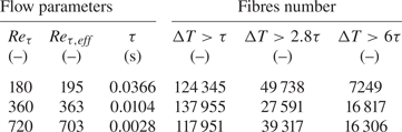
The number of fibres identified and tracked in each experiment is variable and depends on minimum track length considered. Indeed, in order to provide reliable measurements of velocity and rotation rates, the fibres are tracked over a long time interval. This ensures that the fibres reconstructed are not the result of the clustering of tracers or optical noise, but represent physical objects, with a time-persistent shape. The time interval considered for the tracking is defined as a function of the viscous time scale of the flow,  $\tau$, reported in table 2 for all Reynolds numbers considered. The number of fibres tracked at each $ {\textit {Re}}_\tau$ is reported in table 2 for three different values of track length, $\Delta T$, where the track length is defined as the minimum time interval over which the fibre is tracked. It is trivial to observe that, by increasing the track length considered, the number of fibres always decreases. The statistics presented in this work have been obtained accounting for the fibres tracked for $\Delta T>2.8\tau$.
Number of fibres tracked for each Reynolds number ( $ {\textit {Re}}_\tau$) as a function of the track length ( $\Delta T$), i.e. the minimum time interval over which the fibres are tracked. The length of the tracks is specified as a function of the viscous time scale of the flow ( $\tau$).


 Open access

