


1. Introduction
Astarita (Reference Astarita1991) proposed a steady, homogeneous, two-dimensional flow field of the form
 \begin{gather}u = \dot{\gamma }y/(1 + \xi ),\end{gather}
 \begin{gather}v = \xi \dot{\gamma }x/(1 + \xi ),\end{gather}
where u is the velocity in the x direction, v the velocity in the y direction,  $\dot{\gamma }$ is the magnitude of the shear rate and
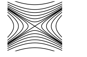
  $\xi $ a flow-type parameter which is +1 for extensional flow, 0 for simple shear and −1 for solid-body rotation as shown in the streamline plots illustrated in figure 1. The streamlines of the Astarita flow field can be calculated via
 \begin{equation}\frac{{{y^2}}}{2} - \xi \frac{{{x^2}}}{2} = C,\end{equation}
where C is a stream function value (constant along a streamline). Thus  $\xi < 0$ leads to so called ‘elliptical’ flows (closed streamlines), simple shear $(\xi = 0)$ gives rise to a series of horizontal lines where the stream function is only a function of y and $\xi > 0$ leads to ‘hyperbolic’ flows where the streamlines are open. Although there are other velocity field formulations where the same families of flows can be achieved (Fuller & Leal Reference Fuller and Leal1980; Wagner & McKinley Reference Wagner and McKinley2016), Astarita's flow field has an interesting feature as the flow field gives rise to the following velocity gradient tensor:
 \begin{equation}\boldsymbol{L} =
\boldsymbol{\nabla }{\boldsymbol{u}^{\boldsymbol{T}}} =
\dot{\gamma }\left[ {\begin{array}{@{}ccc@{}} 0 & {1/(1 + \xi
)} & 0\\ {\xi /(1 + \xi )}& 0& 0\\ 0 & 0 & 0 \end{array}}
\right],\end{equation}
\begin{equation}\boldsymbol{L} =
\boldsymbol{\nabla }{\boldsymbol{u}^{\boldsymbol{T}}} =
\dot{\gamma }\left[ {\begin{array}{@{}ccc@{}} 0 & {1/(1 + \xi
)} & 0\\ {\xi /(1 + \xi )}& 0& 0\\ 0 & 0 & 0 \end{array}}
\right],\end{equation}
such that D, the symmetric rate of deformation tensor, is totally independent of the flow-type parameter for all types of flow  $( - 1 < \xi \le 1)$, i.e.
 \begin{align}
\boldsymbol{D} = \frac{1}{2}\textrm{(}\boldsymbol{\nabla }\boldsymbol{u} +
\boldsymbol{\nabla }{\boldsymbol{u}^{\boldsymbol{T}}}\textrm{)} =
\frac{{\dot{\gamma }}}{2}\left[ {\begin{array}{@{}ccc@{}}
0 & {(1 + \xi )/(1 + \xi )} & 0\\ {(\xi + 1)/(1 + \xi )} & 0 & 0\\
0 & 0 & 0 \end{array}} \right] = \frac{{\dot{\gamma
}}}{2}\left[ {\begin{array}{@{}ccc@{}} 0 & 1 & 0\\ 1 & 0 & 0\\ 0 & 0 & 0
\end{array}} \right].\end{align}
\begin{align}
\boldsymbol{D} = \frac{1}{2}\textrm{(}\boldsymbol{\nabla }\boldsymbol{u} +
\boldsymbol{\nabla }{\boldsymbol{u}^{\boldsymbol{T}}}\textrm{)} =
\frac{{\dot{\gamma }}}{2}\left[ {\begin{array}{@{}ccc@{}}
0 & {(1 + \xi )/(1 + \xi )} & 0\\ {(\xi + 1)/(1 + \xi )} & 0 & 0\\
0 & 0 & 0 \end{array}} \right] = \frac{{\dot{\gamma
}}}{2}\left[ {\begin{array}{@{}ccc@{}} 0 & 1 & 0\\ 1 & 0 & 0\\ 0 & 0 & 0
\end{array}} \right].\end{align}
The Astarita flow field (equation (1.4)) can also be used to illustrate the concept of Tanner & Huilgol (Reference Tanner and Huilgol1975) of so-called ‘strong’ or ‘weak’ flows. In particular, ‘strong’ flow is characterised by at least one positive eigenvalue of L while in a ‘weak’ flow no positive real eigenvalues can occur. The eigenvalues of  $\boldsymbol{L}({\varXi _{\boldsymbol{L}}})$ are given by
 \begin{equation}{\varXi _{\boldsymbol{L}}} \in \left\{ { - \frac{{\dot{\gamma }\sqrt \xi }}{{(1 + \xi )}};0;\frac{{\dot{\gamma }\sqrt \xi }}{{(1 + \xi )}}} \right\},\end{equation}
and thus elliptical flows  $(\xi < 0)$ lead to two imaginary eigenvalues and are strictly weak, simple shear $(\xi = 0)$ leads to three vanishing eigenvalues (a marginal case between weak and strong flow) and hyperbolic flows $(\xi > 0)$ are strong as they have one positive eigenvalue of L, no matter how small the actual value of $\xi $.
Streamlines for the steady and homogeneous ‘Astarita’ flow fields in the limit of (a) solid-body rotation  $(\xi ={-} 1.0)$ or (b) simple shearing $(\xi = 0)$ and (c) planar extension $(\xi ={+} 1.0)$. Note that eigenvectors of D are independent of flow type and aligned with x = ±y.

In this short paper, we investigate the response of commonly used differential viscoelastic constitutive models to this flow field, including the upper and lower convected Maxwell (i.e. the limiting case of the Oldroyd-B/A models in the case of no solvent viscosity; Oldroyd Reference Oldroyd1950), the linear form of the simplified Phan-Thien and Tanner (sPTT) model (Phan-Thien & Tanner Reference Phan-Thien and Tanner1977) and the Giesekus model (Giesekus Reference Giesekus1982). As the flow is steady and homogeneous, the sPTT model results also give the FENE-P model solutions via a simple transformation of parameters (Cruz, Pinho & Oliveira Reference Cruz, Pinho and Oliveira2005; Davoodi et al. Reference Davoodi, Zografos, Oliveira and Poole2022). The response of the models is probed in order to determine how a scalar ‘viscosity’ function may be rigorously constructed which includes flow-type dependence but be otherwise inelastic.
A few previous studies have proposed inelastic models which incorporate flow-type dependence and these approaches have been recently reviewed (Poole Reference Poole2023). Of particular relevance here is the ground-breaking work of Schunk & Scriven (Reference Schunk and Scriven1990) who used the flow-type parameter  ${R_D}$ (due to Astarita Reference Astarita1979), to propose a generalised Newtonian fluid constitutive equation which was a linear combination of two ‘Carreau-type’ equations (e.g. one exhibiting rate thinning for shear and one exhibiting tensioning thickening for extension). For two-dimensional and axisymmetric flows this was given as
 \begin{equation}\eta = {\eta _{SH}}(I{I_D}){R_D} + {\eta _{EX}}(I{I_D})(1 - {R_D}),\end{equation}
where IID is the second invariant of D ( $I{I_D} = tr({\boldsymbol{D}^2})$ and $\dot{\gamma } = \sqrt {2I{I_D}} $). The weighting function ${R_D}$ was then allowed to vary between 1 for simple shear and 0 for pure extension (i.e. limited to ${R_D} \le 1$). Schunk & Scriven (Reference Schunk and Scriven1990) modified ${R_D}$ slightly such that a small parameter is added to it to avoid the ${R_D}$ parameter becoming undefined as the flow tends to solid-body rotation and simply set all locations in the flow where ${R_D} > 1$ to be equivalent to simple shear (i.e. ${R_D} = 1$). Astarita (Reference Astarita1991), in a responsive note to Schunk & Scriven (Reference Schunk and Scriven1990), suggested this approach of limiting ${R_D}$ to be one that was flawed, as it failed to distinguish elliptical motions (i.e. corresponding to solid-body-like flows) from shear and used the response of the upper convected Maxwell (UCM) model to (1.1)–(1.2) to justify this criticism. De Souza Mendes et al. (Reference de Souza Mendes, Padmanabhan, Scriven and Macosko1995) showed that using a modified form of (1.7) which now uses a weighted geometric mean, i.e.
 \begin{equation}\eta = {\eta _{SH}}{(I{I_D})^{{R_D}}} + {\eta _{EX}}{(I{I_D})^{(1 - {R_D})}},\end{equation}
produced viscosities for ‘mixed’ flows less dominated by the extensional viscosity. Equation (1.8) also exhibits viscosities that decrease monotonically with increasing  ${R_D}$ – in agreement with Astarita's (Reference Astarita1991) postulate that it should based on the response of the UCM model – and as ${R_D} \to \infty$ (i.e. as the motion approaches solid-body rotation), the viscosity function approaches zero, and hence the extra stress is assured to approach zero as it should. However, there is no theoretical basis for the dependence of a scalar viscosity function to vary with flow type as postulated in (1.7) and (1.8). For steady homogeneous flows it can be shown that a renormalised version of ${R_D}$ is equivalent to the flow-type parameter (Mompean, Thompson & de Souza Mendes Reference Mompean, Thompson and de Souza Mendes2003) contained within (1.1) and (1.2):
 \begin{equation}\xi = \frac{{1 - {R_D}}}{{1 + {R_D}}} = \frac{{|\boldsymbol{D}|- |\bar{\boldsymbol{W}}|}}{{|\boldsymbol{D}|+ |\bar{\boldsymbol{W}}|}},\end{equation}
where again  $\xi ={+} 1$ corresponds to pure extensional flow, $\xi = 0$ corresponds to simple shear and $\xi ={-} 1$ corresponds to pure rotational flow (here $|\boldsymbol{A}|\equiv \sqrt {2tr({\boldsymbol{A}^2})} $). This arises because in steady homogeneous flow fields the eigenvectors of D do not rotate and then the relative vorticity tensor of Astarita (Reference Astarita1979) $(\bar{\boldsymbol{W}})$ is simply equal to the vorticity tensor $\textrm{(}W = {\textstyle{1 \over 2}}(\boldsymbol{\nabla }{\boldsymbol{u}^T} - \boldsymbol{\nabla }\boldsymbol{u}))$. Outside of steady homogeneous flow, to calculate the relative vorticity tensor $\bar{\boldsymbol{W}}$ then one must firstly determine the rate of rotation of the tensor D at a particle $(\boldsymbol{\varOmega })$. If ${\boldsymbol{e}_i}$ (with i = 1, 2, 3) are the proper vectors of D – i.e. unit vectors along the principal axes of D – the definition of $\boldsymbol{\varOmega }$ is
 \begin{equation}\frac{{\textrm{D}{\boldsymbol{e}_i}}}{{\textrm{D}t}} = \boldsymbol{\varOmega }\boldsymbol{\cdot }{\boldsymbol{e}_i},\end{equation}
where D/Dt is the usual substantial derivative. The relative vorticity tensor  $\bar{\boldsymbol{W}}$ is then defined:
 \begin{equation}\bar{\boldsymbol{W}} = \boldsymbol{W} - \boldsymbol{\varOmega }.\end{equation}
Aside from Astarita's original short note (Astarita Reference Astarita1991) where the response of the UCM model to (1.1) and (1.2) to elliptical motions was shown, we are unaware of any other studies which have probed the response of viscoelastic models to this flow field. Clearly, many previous studies have determined the response of these models to two limiting cases of flow type (i.e. shear  $\xi = 0$ and planar extension $\xi ={+} 1$). Given the ubiquity of such solutions and their textbook nature (Bird, Armstrong & Hassager Reference Bird, Armstrong and Hassager1987; Tanner Reference Tanner2000), we will not discuss these further here (although we confirmed that the solutions obtained here are in agreement with these limiting cases for the models studied). Of closest relevance to the results in the current study is the paper by Lagnado, Phan-Thien & Leal (Reference Lagnado, Phan-Thien and Leal1985), which studied the stability of two-dimensional linear flow fields for models of ‘Oldroyd type’ similar to the flow field of (1.1) and (1.2) but with the extensional/compressional axes aligned with the x and y directions rather than at 45° to them (figure 1). (We note, parenthetically, that in the formulation of Lagnado et al. (Reference Lagnado, Phan-Thien and Leal1985) however, D is not independent of the flow-type parameter.) To study the stability of the flow field, they firstly derived analytical expressions for the stress components and so the UCM/lower convected Maxwell (LCM) results we show here could be obtained from the results of Lagnado et al. (Reference Lagnado, Phan-Thien and Leal1985) via a simple rotation of axes or, as we have actually done, via comparison of invariants of the stress tensor which are obviously independent of the frame of reference.
The rest of the paper is structured as follows. Firstly, we find it instructive to consider the response of a Newtonian fluid to the flow field. We then follow this with a section devoted to the response of the UCM/Oldroyd-B model where analytical results for the various stress tensor components can be determined and several approaches are tested for defining a scalar apparent viscosity function. These results give rise to an intriguing relation between the invariants of the extra stress tensor and this is explored for a broader range of models in the following subsection. The detailed results for the sPTT/FENE-P and Giesekus models are then shown which highlight the need to move to an eigenbasis to define an apparent viscosity. These results are then used to propose a scalar viscosity function as a function of both the shear rate magnitude and the flow-type parameter. In the final section, it is shown how this viscosity model can, in our frame-invariant coordinate system, also be extended to include normal-stress differences. The paper ends with a short conclusions and outlook section.
2. Newtonian fluid response
Before proceeding to analyse the response of viscoelastic models, we find it is firstly worthwhile to understand the response of a simple, Newtonian fluid which is governed by a linear equation for the stress:
 \begin{equation}\boldsymbol{\tau } = 2\eta \boldsymbol{D},\end{equation}
where  $\boldsymbol{\tau }$ is the stress tensor, $\eta $ is the constant viscosity and D is still the rate of deformation tensor. Having already demonstrated that the rate of deformation tensor is independent of the flow-type parameter (equation (1.5)), we immediately see that the stress in a Newtonian fluid for the Astarita flow is also independent of flow type. The result of this invariance means that, in a Newtonian fluid, any scalar viscosity function must be independent of flow type in a steady, homogeneous two-dimensional flow.
Given the linear nature of a Newtonian fluid, it is also possible to make the following observations: (1) the invariants of the stress tensor are simply related to the invariants of the rate of deformation tensor via the multiplier  $2\eta $ (the same must also be true for the eigenvalues of $\boldsymbol{\tau }$ and D); (2) the eigenvectors – i.e. the principal directions – of $\boldsymbol{\tau }$ and D are shared; (3) a corollary of (1) is that, for incompressible materials, in planar flows D has only one non-zero principal invariant (the second invariant; Poole Reference Poole2023) and therefore for Newtonian fluids the same is true of the stress tensor; and (4) a corollary of (3) is that, attempting to define a frame-independent ‘viscosity’ for a Newtonian fluid in an arbitrary steady planar flow, e.g. via taking an invariant measure of the stress and dividing it by an invariant measure of the rate of deformation tensor, will always return a constant value, independent of flow type if the same invariant measures are used for both tensors.
The well-read reader at this point is probably asking themselves what has happened to the well-known ‘Trouton ratios’, i.e. the ratio of an extensional viscosity to a shear viscosity, which are covered in all standard rheology textbooks (e.g. Bird et al. Reference Bird, Armstrong and Hassager1987, p. 39; Barnes, Hutton. & Walters Reference Barnes, Hutton and Walters1989, p. 80) but here appear to be totally missing in action. In Newtonian fluids these are stated ubiquitously to be equal to 3 in uniaxial extensional flow and, of more relevance to the two-dimensional flows considered here, either 4 (or 2) in planar extensional flow (depending on whether the planar viscosity or the so-called ‘cross-viscosity’ is considered; Petrie Reference Petrie1990).
To understand why we do not recover this well-known Trouton ratio for a Newtonian fluid in the planar extension limit (i.e.  $\xi ={+} 1$), we simply have to recall how both shear and extensional viscosities are defined. In so doing, we see they are somehow inconsistent and any consistently defined measure of viscosity would result in a constant value of ‘viscosity’ for a Newtonian fluid independent of flow type in homogeneous, two-dimensional flows, as we have already shown. For example, in a simple shear flow where the flow direction is x, the velocity gradient direction is y and the velocity is u, a fluid's shear viscosity $({\eta _{SH}})$ is defined (Dealy et al. Reference Dealy, Morris, Morrison and Vlassopoulos2013) as the stress in the xy plane $({\tau _{xy}})$ divided by the shear rate $({\dot{\gamma }_{xy}} = \textrm{d}u/\textrm{d}y)$:
 \begin{equation}{\eta _{SH}} = \frac{{{\tau _{xy}}}}{{{{\dot{\gamma }}_{xy}}}},\end{equation}
i.e. one component of the stress tensor being divided by one component of the rate of deformation tensor. As for steady simple shear flow the rate of deformation tensor D is simply
 \begin{equation}2\boldsymbol{D} = \boldsymbol{\nabla }\boldsymbol{u} + \boldsymbol{\nabla }{\boldsymbol{u}^{\boldsymbol{T}}} = \dot{\gamma }\left[ {\begin{array}{@{}cc@{}} 0 & 1\\ 1 & 0 \end{array}} \right],\end{equation}
and the magnitude  $(\sqrt {2\textrm{tr}(\boldsymbol{D}.\boldsymbol{D})} )$ is simply $\dot{\gamma }$. In contrast, in a planar extensional flow where now the flow direction is x′, the velocity is u′ but the extensional viscosity $({\eta _{EX}})$ is defined by a normal stress difference $({\tau _{x^{\prime}x^{\prime}}} - {\tau _{y^{\prime}y^{\prime}}})$ divided by the strain rate $({\dot{\varepsilon }_{x^{\prime}x^{\prime}}} = \textrm{d}u^{\prime}/\textrm{d}\kern0.7pt x^{\prime})$, i.e.
 \begin{equation}{\eta _{EX}} = \frac{{{\tau _{x^{\prime}x^{\prime}}} - {\tau _{y^{\prime}y^{\prime}}}}}{{{{\dot{\varepsilon }}_{x^{\prime}x^{\prime}}}}}.\end{equation}
For ‘classical’ planar extensional flow for an incompressible material (i.e. du′/dx′ = −dv′/dy′) the rate of deformation tensor D is now
 \begin{equation}2\boldsymbol{D} =
\boldsymbol{\nabla }\boldsymbol{u} + \boldsymbol{\nabla
}{\boldsymbol{u}^{\boldsymbol{T}}}\textrm{\; =
2}{\dot{\varepsilon }_{x^{\prime}x^{\prime}}}\left[
{\begin{array}{@{}cc@{}} 1 & 0\\ 0 & { - 1} \end{array}}
\right],\end{equation}
\begin{equation}2\boldsymbol{D} =
\boldsymbol{\nabla }\boldsymbol{u} + \boldsymbol{\nabla
}{\boldsymbol{u}^{\boldsymbol{T}}}\textrm{\; =
2}{\dot{\varepsilon }_{x^{\prime}x^{\prime}}}\left[
{\begin{array}{@{}cc@{}} 1 & 0\\ 0 & { - 1} \end{array}}
\right],\end{equation}
i.e. now the magnitude of D is  $2{\dot{\varepsilon }_{x^{\prime}x^{\prime}}}$. Thus, inconsistent scalar magnitudes are being used for the deformation rate between shear and extensional viscosity definitions and this gives rise to a factor of two difference in the viscosity so determined. Finally, as the stress in each case is plane, we can use plane stress transformative rules (Boresi & Schmidt Reference Boresi and Schmidt2002) to show that rotating from the principal axes of extensional flow (x′ and y′) back to the shear flow axes (x, y) gives a relationship between the shear stress and the normal stress difference in each frame:
 \begin{equation}{\tau _{xy}} = {\textstyle{1 \over 2}}({\tau _{x^{\prime}x^{\prime}}} - {\tau _{y^{\prime}y^{\prime}}}),\end{equation}
which shows where the remaining factor of two comes from in the Trouton ratio. If the shear and extensional viscosities were defined consistently, either as the ratio of the magnitude of the stress divided by the magnitude of the rate of deformation tensor or as the first normal-stress difference in a frame aligned with the principal axis divided by the magnitude of the rate of deformation tensor, then the ‘viscosity’ so defined would be identical in each case.
Finally, simple shearing can be decomposed into a locally rotating (solid-body) component and a straining/purely planar extensional flow oriented at 45° to the flow direction (Duprat & Stone Reference Duprat and Stone2016) and is often thought of in this manner (Mackley Reference Mackley2010). As the Newtonian constitutive equation is linear, this decomposition means that the stress from simple shear must then be equal to the stress in planar extension plus the stress due to solid-body rotation. As, by definition, no viscous stress is produced in a fluid undergoing solid-body rotation (i.e. D = 0) then the stress in simple shear for a Newtonian fluid must be equal to the stress in planar extension.
3. Oldroyd-B/UCM model response
Having shown the response of a Newtonian fluid, we now proceed to the Oldroyd-B model as this represents the backbone of all the models we study in the remainder of the main body of the paper (Bird et al. Reference Bird, Armstrong and Hassager1987). In fact, we limit our investigations in this paper to cases of no solvent viscosity contribution to the stress – as we have just shown that this Newtonian solvent viscosity contribution is independent of flow type – and therefore we are studying the so-called UCM model (Oldroyd Reference Oldroyd1950):
 \begin{equation}\boldsymbol{\tau } +
\lambda \mathop{\boldsymbol{\tau }}\limits^\nabla = 2{\eta
_p}\boldsymbol{D},\end{equation}
\begin{equation}\boldsymbol{\tau } +
\lambda \mathop{\boldsymbol{\tau }}\limits^\nabla = 2{\eta
_p}\boldsymbol{D},\end{equation}
where  ${\eta _p}$ is the polymeric viscosity, $\lambda$ is the relaxation time and the operator acting on the second term represents Oldroyd's upper convected (‘contravariant’) derivative:
 \begin{equation}\mathop{\boldsymbol{\tau }}\limits^\nabla = \frac{{\textrm{D}\boldsymbol{\tau }}}{{\textrm{D}t}} - {(\boldsymbol{\nabla }\boldsymbol{u})^T}\boldsymbol{\cdot }\boldsymbol{\tau } - (\boldsymbol{\tau }\boldsymbol{\cdot }(\boldsymbol{\nabla }\boldsymbol{u})).\end{equation}
Combining this derivative operator with the definitions of the velocity gradient and its transpose,
 \begin{align}\boldsymbol{\nabla
}{\boldsymbol{u}^{\boldsymbol{T}}} = \dot{\gamma }\left[
{\begin{array}{@{}cc@{}} 0 & {1/(1 + \xi )}\\ {\xi /(1 + \xi
)} & 0 \end{array}} \right],\quad \boldsymbol{\nabla
}\boldsymbol{u} = \dot{\gamma }\left[
{\begin{array}{@{}cc@{}} 0 & {\xi /(1 + \xi )}\\ {1/(1 + \xi
)} & 0 \end{array}} \right],\end{align}
\begin{align}\boldsymbol{\nabla
}{\boldsymbol{u}^{\boldsymbol{T}}} = \dot{\gamma }\left[
{\begin{array}{@{}cc@{}} 0 & {1/(1 + \xi )}\\ {\xi /(1 + \xi
)} & 0 \end{array}} \right],\quad \boldsymbol{\nabla
}\boldsymbol{u} = \dot{\gamma }\left[
{\begin{array}{@{}cc@{}} 0 & {\xi /(1 + \xi )}\\ {1/(1 + \xi
)} & 0 \end{array}} \right],\end{align}
together with the constitutive equation (3.1) gives rise to the following five equations for the various stress components:
 \begin{gather}{\tau _{xy}} - \lambda \dot{\gamma }(1/(1 + \xi )){\tau _{yy}} - \lambda \dot{\gamma }(\xi /(1 + \xi )){\tau _{xx}} = {\eta _p}\dot{\gamma },\end{gather}
 \begin{gather}{\tau _{yx}} - \lambda \dot{\gamma }(\xi /(1 + \xi )){\tau _{xx}} - \lambda \dot{\gamma }(1/(1 + \xi )){\tau _{yy}} = {\eta _p}\dot{\gamma },\end{gather}
 \begin{gather}{\tau _{xx}} - \lambda \dot{\gamma }(1/(1 + \xi )){\tau _{xy}} - \lambda \dot{\gamma }{\tau _{xy}}(1/(1 + \xi )) = 0,\end{gather}
 \begin{gather}{\tau _{yy}} - \lambda \dot{\gamma }(\xi /(1 + \xi )){\tau _{xy}} - \lambda \dot{\gamma }{\tau _{xy}}(\xi /(1 + \xi )) = 0,\end{gather}
 \begin{gather}{\tau _{zz}} = 0.\end{gather}
From (3.4a) and (3.4b), we see the inherent symmetry of the stress tensor. Rearranging (3.4c) and (3.4d) we get the normal stress components as a function of the shear stress:
 \begin{gather}{\tau _{xx}} = 2\lambda \dot{\gamma }\left( {\frac{1}{{1 + \xi }}} \right){\tau _{xy}},\end{gather}
 \begin{gather}{\tau _{yy}} = 2\lambda \dot{\gamma }\left( {\frac{\xi }{{1 + \xi }}} \right){\tau _{xy}},\end{gather}
then substitution of (3.5a) and (3.5b) into (3.4a) gives an explicit equation for the shear stress:
 \begin{equation}{\tau _{xy}} = \frac{{{\eta _p}\dot{\gamma }}}{{\left[ {1 - 4{{(\lambda \dot{\gamma })}^2}\left( {\dfrac{1}{{1 + \xi }}} \right)\left( {\dfrac{\xi }{{1 + \xi }}} \right)} \right]}},\end{equation}
which is in agreement with the original paper of Astarita (Reference Astarita1991). As the Astarita flow field is steady and homogeneous and we are restricted here to incompressible materials, the extra stress is divergence-free and therefore does not enter the momentum equation. Therefore the extra stress field is completely determined by (3.6) and the first and second normal-stress differences which here we define as
 \begin{equation}
\left. {\begin{array}{c@{}} {{N_1} = {\tau_{xx}} - {\tau_{yy}}
= 2\lambda \dot{\gamma }\left( {\dfrac{{1 - \xi }}{{1 + \xi
}}} \right){\tau_{xy}},}\\ {{N_2} = {\tau_{yy}} -
{\tau_{zz}} = 2\lambda \dot{\gamma }\left( {\dfrac{\xi }{{1
+ \xi }}} \right){\tau_{xy}}.} \end{array}}
\right\}\end{equation}
\begin{equation}
\left. {\begin{array}{c@{}} {{N_1} = {\tau_{xx}} - {\tau_{yy}}
= 2\lambda \dot{\gamma }\left( {\dfrac{{1 - \xi }}{{1 + \xi
}}} \right){\tau_{xy}},}\\ {{N_2} = {\tau_{yy}} -
{\tau_{zz}} = 2\lambda \dot{\gamma }\left( {\dfrac{\xi }{{1
+ \xi }}} \right){\tau_{xy}}.} \end{array}}
\right\}\end{equation}
In addition, the pressure variation (up to an isotropic constant) can be determined from the momentum equation in combination with (1.1) and (1.2). In the shear-flow case  $(\xi = 0)$ the pressure field is also homogeneous. For steady simple shear, (3.6) and (3.7) give the well-known solution:
 \begin{equation}{\tau _{xy}} = {\eta _p}\dot{\gamma },\quad {\tau _{xx}} = 2\lambda \dot{\gamma }{\tau _{xy}} = 2\lambda {\eta _p}{\dot{\gamma }^2},\quad {\tau _{yy}} = 0,\end{equation}
such that the shear viscosity (defined as in (2.2)) is constant, the first normal-stress difference  $({\tau _{xx}} - {\tau _{yy}})$ goes quadratically with shear rate and the second normal-stress difference $({\tau _{yy}} - {\tau _{zz}})$ is identically zero. In planar extensional flow $(\xi ={+} 1)$ the stresses all become singular at $\lambda \dot{\gamma } = 1$:
 \begin{equation}\left.
{\begin{array}{c@{}} {{\tau_{xy}} =
\dfrac{{{\eta_p}\dot{\gamma }}}{{[1 - {{(\lambda
\dot{\gamma })}^2}]}},}\\ {{\tau_{xx}} = {\tau_{yy}} =
\lambda \dot{\gamma }{\tau_{xy}}.} \end{array}}
\right\}\end{equation}
\begin{equation}\left.
{\begin{array}{c@{}} {{\tau_{xy}} =
\dfrac{{{\eta_p}\dot{\gamma }}}{{[1 - {{(\lambda
\dot{\gamma })}^2}]}},}\\ {{\tau_{xx}} = {\tau_{yy}} =
\lambda \dot{\gamma }{\tau_{xy}}.} \end{array}}
\right\}\end{equation}
In fact, it is noticeable that for any flow with an extensional component – what Tanner & Huilgol (Reference Tanner and Huilgol1975) characterised as a ‘strong’ flow as already discussed – the stress becomes singular at a critical strain rate corresponding to
 \begin{equation}\xi > 0,\quad {\dot{\gamma }_{cr}} = \frac{1}{{2\lambda }}\sqrt {\frac{{{{(1 + \xi )}^2}}}{\xi }} .\end{equation}
Finally, for what Astarita called ‘elliptical’ motions with  $\xi < 0$, which reach the solid-body limit at $\xi ={-} 1$, we observe rate thinning of all the stress components and, as we approach the solid-body limit, we achieve the following asymptotic variation of an apparent viscosity (defined as in (2.2) which is, of course, only formally valid for simple shear flow and hence the ‘apparent’ terminology, where $\xi + 1 = \varDelta $):
 \begin{equation}{\eta _{\dot{\gamma } \gg 1}} = \frac{{{\varDelta ^2}{\eta _p}}}{{4{{(\lambda \dot{\gamma })}^2}}}\sim {\dot{\gamma }^{ - 2}} \to 0.\end{equation}
Figure 2(a) plots the variation of such an apparent viscosity as a function of non-dimensional strain rate  $(\lambda \dot{\gamma })$ – essentially a Weissenberg number in this rheologically steady flow (Poole Reference Poole2012) – for simple shearing and two elliptical flows $(\xi ={-} 0.5,\; - 0.99)$ highlighting the rate-thinning nature of the Oldroyd-B model in the latter cases. Figure 2(b) shows the variation of the apparent viscosity for all positive $\xi $ cases exhibiting identical self-similar, singular behaviour when the shear rate is normalised by the critical strain rate given in (3.10).
Variation of the stress component  ${\tau _{xy}}$ divided by the shear rate for the Oldroyd-B model (UCM) in (a) steady simple shearing and ‘elliptical’ motions approaching solid-body rotation and (b) all ‘strong’ flows containing finite extensional deformation where the shear rate has now been normalised with the ‘critical’ strain rate (equation (3.10)) at which this stress component goes singular. For this model fluid, G = 1 Pa and λ = 1 s.

Although the Astarita flow for the Oldroyd-B model is completely determined by just three equations, i.e. (3.6) for the shear stress and (3.7a) and (3.7b) for the normal-stress differences, this formalism is perhaps not so helpful outside of simple shearing where the use of such viscometric functions is standard and mainly well understood (Maklad & Poole Reference Maklad and Poole2021). For example, in elliptical flows in addition to the apparent viscosity being rate thinning, N 1 is positive and N 2 is negative, whereas for flows with an extensional component N 1 decreases in importance and N 2 increases in importance such that at  $\xi = 0.5$, N 1 = N 2 (and both are positive) whilst in the pure extension limit N 1 = 0 and N 2 is positive. As N 1 and N 2 are coupled to ${\tau _{xy}}$, all terms go singular at the critical strain rate (equation (3.10)).
If we wish to construct an apparent viscosity from these stress fields, a seemingly fatal issue in the use of (3.6) and (3.7) would be that they are apparently frame dependent and, therefore, a rigid rotation of our axes will give different results. Hence it seems logical to investigate the use of invariant measures of the stress field with which to construct an apparent viscosity function. Given that the stress field is symmetric, and  ${\tau _{zz}}$ is identically zero, there are only two independent principal invariants, namely
 \begin{equation}\left.
{\begin{array}{c@{}} {{I_1} = tr(\boldsymbol{\tau }) =
{\tau_{xx}} + {\tau_{yy}},}\\ {{I_2} = {\textstyle{1 \over
2}}({{(tr(\boldsymbol{\tau }))}^2} - tr({\boldsymbol{\tau
}^2})) = {\tau_{xx}}{\tau_{yy}} - \tau_{xy}^2}
\end{array}} \right\}\end{equation}
\begin{equation}\left.
{\begin{array}{c@{}} {{I_1} = tr(\boldsymbol{\tau }) =
{\tau_{xx}} + {\tau_{yy}},}\\ {{I_2} = {\textstyle{1 \over
2}}({{(tr(\boldsymbol{\tau }))}^2} - tr({\boldsymbol{\tau
}^2})) = {\tau_{xx}}{\tau_{yy}} - \tau_{xy}^2}
\end{array}} \right\}\end{equation}
(one could also use other invariants (I, II) (Bird et al. Reference Bird, Armstrong and Hassager1987) but these can be expressed simply in terms of the principal invariants as  $I = {I_1}$, $II = I_1^2 - 2{I_2}$). Here we are treating the stress tensor $\boldsymbol{\tau }$ as the ‘extra’ stress, i.e. with the pressure handled separately (alternatively, if we assume the flow is also inertialess, then these homogeneous flows give rise to an isotropic pressure which we can arbitrarily set to zero). We note also that I 1 is the equivalent to the sum of the eigenvalues whereas I 2 is the product of the two eigenvalues. Expressed in terms of the principal invariants the eigenvalues of the stress ( $\varXi$) are ${\varXi _1} = 1/2\left[ {{I_1} + \sqrt {I_1^2 - 4{I_2}} } \right]$ and ${\varXi _2} = 1/2\left[ {{I_1} - \sqrt {I_1^2 - 4{I_2}} } \right]$.
Taking inspiration from generalised Newtonian fluids, where the second invariant of D is utilised to determine a magnitude/scalar shear rate, we define an apparent viscosity based on a stress calculated from I 2 as
 \begin{equation}\|\boldsymbol{\tau }\| =
\sqrt { - {I_2}}
,\end{equation}
\begin{equation}\|\boldsymbol{\tau }\| =
\sqrt { - {I_2}}
,\end{equation}which gives an apparent viscosity as
 \begin{equation}{\eta _{ap}} = \frac{\|\boldsymbol{\tau }\|}{{\dot{\gamma }}}.\end{equation}
For the UCM, in simple shearing this returns the ‘usual’ constant viscosity  $({\eta _{ap}} = {\eta _p})$, whereas in pure extensional flow the apparent viscosity is now
 \begin{equation}{\eta _{ap}} = \frac{\|\boldsymbol{\tau }\|}{{\dot{\gamma }}} = \frac{{{\eta _p}}}{{\sqrt {[1 - {{(\lambda \dot{\gamma })}^2}]} }},\end{equation}
which is clearly similar (though not identical) to a viscosity based on (3.9a) although the apparent viscosity defined in (3.14) is now a frame-independent quantity.
Using this measure of apparent viscosity it is possible to show the effect of flow-type parameter as is done in figure 3. At a Weissenberg number  $( = \lambda \dot{\gamma })$ of 0.5, figure 3(a) shows that there is an approximately linear growth in the viscosity between the solid-body limit and the shear-flow limit, followed by a more modest flow-type thickening caused by extension, such that the planar extensional viscosity is about 20 % higher than the shear viscosity. In contrast, at a Weissenberg number much closer to the critical value in planar extension, a much stronger extension thickening is observed with the inclusion of an extensional component. In Appendix A we show that the response of the Oldroyd-A/LCM is essentially identical to the UCM (the only difference being the sign of I 1). Given the singular behaviour of the Oldroyd-B/A models that we have demonstrated for any ‘strong’ flow, i.e. $\xi > 0$, we need to probe models which include finite extensibility before investigating flow-type dependence across an arbitrary large range of shear rate.
Variation of an ‘apparent’ viscosity – defined using (3.14) – with flow-type parameter for the UCM model in the Astarita flow for (a) a Weissenberg number well below critical conditions (Wi = 0.5) and (b) a Weissenberg number close to the critical value (WiCR = 1) where the apparent viscosity becomes unbounded in planar flow (Wi = 0.99). The thinning nature of elliptical motions (ξ < 0) and thickening nature of extensional motions (ξ > 0) are readily apparent. For this model fluid, G = 1 Pa and λ = 1 s.

3.1. Relationships between stress invariants
The ability to relate a supposedly purely viscous stress contribution from the second invariant of the stress tensor (i.e. I 2 in (3.13)), coupled with the separation in simple shearing for the Oldroyd-B model into an ‘elastic’ contribution from I 1 (∝ λ ((3.16a) when  $\xi = 0$)) and a ‘viscous’ contribution from I 2 (∝ ${\eta _p}$((3.16b) when $\xi = 0$)), one might naively wonder if each invariant could be related to either a ‘viscous’ stress or an ‘elastic’ stress component more generally for other flow types. However, it is possible to show that, for the Astarita flow,
 \begin{equation}
\left. {\begin{array}{c@{}} {{I_1} = \dfrac{{2\lambda
{\eta_p}{{\dot{\gamma }}^2}{{(1 + \xi )}^2}}}{{{{(1 + \xi
)}^2} - {{(2\lambda \dot{\gamma })}^2}\xi }},}\\ {{I_2} =
\dfrac{{ - {{({\eta_p}\dot{\gamma })}^2}{{(1 + \xi
)}^2}}}{{{{(1 + \xi )}^2} - {{(2\lambda \dot{\gamma
})}^2}\xi }},} \end{array}} \right\}\end{equation}
\begin{equation}
\left. {\begin{array}{c@{}} {{I_1} = \dfrac{{2\lambda
{\eta_p}{{\dot{\gamma }}^2}{{(1 + \xi )}^2}}}{{{{(1 + \xi
)}^2} - {{(2\lambda \dot{\gamma })}^2}\xi }},}\\ {{I_2} =
\dfrac{{ - {{({\eta_p}\dot{\gamma })}^2}{{(1 + \xi
)}^2}}}{{{{(1 + \xi )}^2} - {{(2\lambda \dot{\gamma
})}^2}\xi }},} \end{array}} \right\}\end{equation}
and therefore the invariants are linearly related via the relationship
 \begin{equation}\frac{{{I_2}}}{{{I_1}}} ={-} \frac{{{\eta _p}}}{{2\lambda }} ={-} \frac{G}{2}.\end{equation}
For steady, homogeneous flow, for the Oldroyd-B model, the stress invariants are independent of flow type and shear rate and simply related to a material property (the modulus G). Essentially the same information is ‘encoded’ in either invariant. For example, often polymeric models are solved in conformation tensor form (Grmela & Carreau Reference Grmela and Carreau1987; Hulsen Reference Hulsen1990) and in this formulation the trace of the conformation tensor is often used to represent the amount of stretching (Vaithianathan & Collins Reference Vaithianathan and Collins2003; Xi & Graham Reference Xi and Graham2009; Pereira et al. Reference Pereira, Mompean, Thais and Thompson2017). The result of (3.17) would say that the second invariant of the conformation tensor gives exactly the same information, at least in the two-dimensional, homogeneous and steady flows studied here. Indeed, one could use the result given in (3.17) to highlight regions in a complex two-dimensional Eulerian steady flow, e.g. in an abrupt contraction, which are in this sense rheologically ‘unsteady’.
Given the simplicity of (3.17), it seems somewhat surprising that it appears to be new to the literature. It is straightforward to show that, even for the UCM model, it does not hold more broadly in other flows; for example in shear start-up although it must asymptote at long times to (3.17) (i.e. when steady state is reached), at short times I 2/I 1 = −G. Likewise in steady uniaxial extensional flow the ratio I 2/I 1 does not become independent of rate but is given by
 \begin{equation}\frac{{{I_2}}}{{{I_1}}} ={-} \frac{G}{2}\left[ {\frac{{1 + 2\lambda \dot{\varepsilon }}}{{1 + \lambda \dot{\varepsilon }}}} \right],\end{equation}
i.e. at low rates (3.17) is recovered but at high rates the ratio tends to −G.
To probe the universality, or otherwise, of this relationship in steady, homogeneous, planar flow we can use the results of Lagnado et al. (Reference Lagnado, Phan-Thien and Leal1985) who used an ‘Oldroyd-type’ constitutive equation which, in the limit of no solvent viscosity and using our notation, is given by
 \begin{equation}\boldsymbol{\tau } + \lambda \left[ {\frac{{\delta \boldsymbol{\tau }}}{{\delta t}} - \beta (\boldsymbol{D}\boldsymbol{\cdot }\boldsymbol{\tau } + \boldsymbol{\tau }\boldsymbol{\cdot }\boldsymbol{D})} \right] = 2{\eta _p}\boldsymbol{D},\end{equation}
where
 \begin{equation}\frac{{\delta \boldsymbol{\tau }}}{{\delta t}} = \frac{{\textrm{D}\boldsymbol{\tau }}}{{\textrm{D}t}} - \boldsymbol{W}\boldsymbol{\cdot }\boldsymbol{\tau + \tau }\boldsymbol{\cdot }\boldsymbol{W}\end{equation}
is a co-rotational (Jaumann) derivative (Bird et al. Reference Bird, Armstrong and Hassager1987). The β parameter acts like a ‘slip’ parameter such that when β = 1 the derivative operator is upper convected, when β = −1 it is lower convected (although Lagnado et al. (Reference Lagnado, Phan-Thien and Leal1985) actually limit β to the range 0 ≤ β ≤ 1) and when β = 0 it is co-rotational. The model of Lagnado et al. shares similarities with the model due to Johnson & Segalman (Reference Johnson and Segalman1977). The relationship between the stress invariants for the Lagnado et al. (Reference Lagnado, Phan-Thien and Leal1985) results can be shown to be
 \begin{equation}\frac{{{I_2}}}{{{I_1}}} ={-} \frac{{{\eta _p}}}{{2\lambda }} ={-} \frac{G}{{2\beta }},\end{equation}
which agrees with our results for the UCM when β = 1 (and for the Oldroyd-A model in Appendix A when β = −1). These results show that although non-affine deformation (‘slip’) does have an impact on the relationship between the stress invariants, via the nature of the convected derivative used in the β parameter, there still exists a very simple linear relationship between them, independent of applied shear rate or flow type. We note, in the co-rotational limit (β = 0), there is no such relationship, however.
As we have already made use of the plane stress transformation rules (see § 2), that show a plane stress field can be converted from extensional to shear by a simple rigid rotation of the axes, perhaps it is not so surprising that the ratio of stress invariants is independent of flow type in a planar flow. However, if we accept this as being true for all models, we need only determine the relationship between invariants in planar extensional flow (using the ‘classical’ definition given in (2.5)). In this way, we have the benefit that the ratio of the invariants becomes simply
 \begin{equation}\frac{{{I_2}}}{{{I_1}}} = \frac{{{\tau _{x^{\prime}x^{\prime}}}{\tau _{y^{\prime}y^{\prime}}}}}{{{\tau _{x^{\prime}x^{\prime}}} + {\tau _{y^{\prime}y^{\prime}}}}}.\end{equation}
For example, for the UCM model we can easily show for planar extensional flow that
 \begin{gather}{\tau _{x^{\prime}x^{\prime}}} - 2\lambda {\dot{\varepsilon }_{x^{\prime}x^{\prime}}}{\tau _{x^{\prime}x^{\prime}}} = 2{\eta _p}{\dot{\varepsilon }_{x^{\prime}x^{\prime}}},\end{gather}
 \begin{gather}{\tau _{y^{\prime}y^{\prime}}} + 2\lambda {\dot{\varepsilon }_{x^{\prime}x^{\prime}}}{\tau _{y^{\prime}y^{\prime}}} ={-} 2{\eta _p}{\dot{\varepsilon }_{x^{\prime}x^{\prime}}},\end{gather}
and then
 \begin{equation}\frac{{{I_2}}}{{{I_1}}} ={-} \frac{{{\eta _p}}}{{2\lambda }} ={-} \frac{G}{2},\end{equation}
i.e. in exact agreement with (3.17).
Moving now to more complex models which can capture shear thinning and bounded extensional viscosity, e.g. for the sPTT model (Phan-Thien & Tanner Reference Phan-Thien and Tanner1977), given by
 \begin{equation}{f_s}\boldsymbol{\tau } + \lambda \mathop{\boldsymbol{\tau }}\limits^\nabla = 2{\eta _p}\boldsymbol{D},\end{equation}
where
 \begin{equation}{f_s} = 1 + \frac{{\lambda \epsilon }}{{{\eta _P}}}tr(\boldsymbol{\tau }),\end{equation}
where  $tr(\boldsymbol{\tau })$ is defined in (3.12a). For classical planar extension for the sPTT model, we have
 \begin{equation}{f_s}{\tau _{x^{\prime}x^{\prime}}} - 2\lambda {\dot{\varepsilon }_{x^{\prime}x^{\prime}}}{\tau _{x^{\prime}x^{\prime}}} = 2{\eta _p}{\dot{\varepsilon }_{x^{\prime}x^{\prime}}},\end{equation}
 \begin{equation}{f_s}{\tau _{y^{\prime}y^{\prime}}} + 2\lambda {\dot{\varepsilon }_{x^{\prime}x^{\prime}}}{\tau _{y^{\prime}y^{\prime}}} ={-} 2{\eta _p}{\dot{\varepsilon }_{x^{\prime}x^{\prime}}}.\end{equation}
Multiplying (3.27a) by  ${\tau _{y^{\prime}y^{\prime}}}$, (3.27b) by ${\tau _{x^{\prime}x^{\prime}}}$ and then taking the difference between the resulting equations, we can eliminate ${f_s}$ and arrive at
 \begin{equation}4\lambda {\dot{\varepsilon }_{x^{\prime}x^{\prime}}}{\tau _{y^{\prime}y^{\prime}}}{\tau _{x^{\prime}x^{\prime}}} ={-} 2{\eta _p}{\dot{\varepsilon }_{x^{\prime}x^{\prime}}}({\tau _{y^{\prime}y^{\prime}}} + {\tau _{x^{\prime}x^{\prime}}}).\end{equation}
Therefore,
 \begin{equation}{\tau _{y^{\prime}y^{\prime}}}{\tau _{x^{\prime}x^{\prime}}} ={-} \frac{G}{2}({\tau _{y^{\prime}y^{\prime}}} + {\tau _{x^{\prime}x^{\prime}}}),\end{equation}
which is exactly the same result as (3.17) (i.e. I 2/I 1 = −G/2) once again (given (3.22)). Given the equivalence between the sPTT and FENE-P models (Cruz et al. Reference Cruz, Pinho and Oliveira2005; Davoodi et al. Reference Davoodi, Zografos, Oliveira and Poole2022) in steady homogeneous flows, this simple result also holds for that model.
Finally, we consider the Giesekus (Reference Giesekus1982) model, defined as
 \begin{equation}\boldsymbol{\tau } + \lambda \mathop{\boldsymbol{\tau }}\limits^\nabla \; + \; \frac{{\alpha \lambda }}{{{\eta _p}}}{\boldsymbol{\tau }^2} = 2{\eta _p}\boldsymbol{D},\end{equation}
where  $\alpha $ is the so-called mobility parameter, which must remain less than 0.5 for the stress to remain monotonic in steady simple shearing. For classical planar extension for the Giesekus model, we have
 \begin{gather}{\tau _{x^{\prime}x^{\prime}}} - 2\lambda {\dot{\varepsilon }_{x^{\prime}x^{\prime}}}{\tau _{x^{\prime}x^{\prime}}} + \frac{{\alpha \lambda }}{{{\eta _p}}}\tau _{x^{\prime}x^{\prime}}^2 = 2{\eta _p}{\dot{\varepsilon }_{x^{\prime}x^{\prime}}},\end{gather}
 \begin{gather}{\tau _{y^{\prime}y^{\prime}}} + 2\lambda {\dot{\varepsilon }_{x^{\prime}x^{\prime}}}{\tau _{y^{\prime}y^{\prime}}} + \frac{{\alpha \lambda }}{{{\eta _p}}}\tau _{y^{\prime}y^{\prime}}^2 ={-} 2{\eta _p}{\dot{\varepsilon }_{x^{\prime}x^{\prime}}}.\end{gather}
These two quadratic equations can be solved to show that in the limit  $\lambda {\dot{\varepsilon }_{x^{\prime}x^{\prime}}} \ll 1$ then
 \begin{equation}\frac{{{I_2}}}{{{I_1}}} \to - \frac{G}{{2(1 - \alpha )}},\end{equation}
whilst for  $\lambda {\dot{\varepsilon }_{x^{\prime}x^{\prime}}} \gg 1$ this becomes
 \begin{equation}\frac{{{I_2}}}{{{I_1}}} \to - G.\end{equation}
Having shown the very simple linear relationships which relate the two stress invariants for a range of models, we now show what the complete stress field looks like for the sPTT/FENE-P and Giesekus models.
4. Simplified Phan-Thien and Tanner model (linear form) response
Combining the velocity gradient (and its transpose) of the Astarita flow, (3.3), with the sPTT constitutive equation, (3.25) and (3.26), gives rise to the following equations for the stress components (note  ${\tau _{zz}} = 0$ and ${\tau _{yx}} = {\tau _{xy}}$):
 \begin{gather}{f_s}{\tau _{xy}} - \lambda \dot{\gamma }(1/(1 + \xi )){\tau _{yy}} - \lambda \dot{\gamma }(\xi /(1 + \xi )){\tau _{xx}} = {\eta _p}\dot{\gamma },\end{gather}
 \begin{gather}{f_s}{\tau _{xx}} = 2\lambda \dot{\gamma }{\tau _{xy}}(1/(1 + \xi )),\end{gather}
 \begin{gather}{f_s}{\tau _{yy}} = 2\lambda \dot{\gamma }{\tau _{xy}}(\xi /(1 + \xi )).\end{gather}
Dividing (4.1c) by (4.1b) gives
 \begin{equation}{\tau _{yy}} = \xi {\tau _{xx}}.\end{equation}
Substitution of (4.2) and (4.1b) into (4.1a) then gives the following cubic for  ${\tau _{xx}}$:
 \begin{align}\frac{{{{(1 + \xi
)}^3}}}{{2\lambda \dot{\gamma }}}{\left( {\frac{{\lambda
\epsilon }}{{{\eta_p}}}} \right)^2}\tau _{xx}^3 +
\frac{{{{(1 + \xi )}^2}}}{{2\lambda \dot{\gamma }}}\left(
{\frac{{\lambda \epsilon }}{{{\eta_p}}}} \right)\tau
_{xx}^2 + \left[ {\frac{{(1 + \xi )}}{{2\lambda \dot{\gamma }}} - \frac{{2\lambda \dot{\gamma \xi}
}}{{(1 + \xi )}}} \right]{\tau _{xx}} - {\eta
_p}\dot{\gamma } = 0.\end{align}
\begin{align}\frac{{{{(1 + \xi
)}^3}}}{{2\lambda \dot{\gamma }}}{\left( {\frac{{\lambda
\epsilon }}{{{\eta_p}}}} \right)^2}\tau _{xx}^3 +
\frac{{{{(1 + \xi )}^2}}}{{2\lambda \dot{\gamma }}}\left(
{\frac{{\lambda \epsilon }}{{{\eta_p}}}} \right)\tau
_{xx}^2 + \left[ {\frac{{(1 + \xi )}}{{2\lambda \dot{\gamma }}} - \frac{{2\lambda \dot{\gamma \xi}
}}{{(1 + \xi )}}} \right]{\tau _{xx}} - {\eta
_p}\dot{\gamma } = 0.\end{align}
To solve (4.3), Cardano's formula can be used when  $\xi \le 0$; however, for cases containing some extension (i.e. $\xi > 0$) this method no longer works and we may use the trigonometric solution for cubic equations which works for nearly all extensibility values in this regime (Zwillinger Reference Zwillinger2012). We also solved (4.3) numerically to confirm the correctness of the solutions obtained. In any of these methods, once ${\tau _{xx}}$ is known for a given value of Weissenberg number and flow type, then (4.2) gives ${\tau _{yy}}$ and then (4.1a) gives ${\tau _{xy}}$.
Figure 4 shows the results for the sPTT model for  $\epsilon = 0.01$. Figures 4(a) and 4(b) provide results for the shear viscosity determined via ${\tau _{xy}}$ (equation (2.2)) and $\|\boldsymbol{\tau }\|$ (equation (3.13)), respectively. As N 2 = 0 for the sPTT in steady simple shearing, these two results are identical (and we confirmed that this viscosity is identical to the existing results in shear flow; e.g. Carew, Townsend & Webster Reference Carew, Townsend and Webster1993). Figures 4(c) and 4(d) show the results for the ‘viscosity’ so determined using the same two measures but for elliptical motions tending to solid-body rotation (i.e. $\xi ={-} 0.99$). We note these are not identical but rate thinning is clear in each case. In figure 4(e) we plot the viscosity in extensional flow $\xi = 1$ determined via I 2 and we see the behaviour is not as expected: the ‘viscosity’ goes through a maximum and then thins rather than asymptoting to a constant as the simplified linear model is known to do (Tanner Reference Tanner2000; Davoodi et al. Reference Davoodi, Zografos, Oliveira and Poole2022). To recover such behaviour we can use a viscosity based on a modified form of the Frobenius norm of the stress $({\|\boldsymbol{\tau }\|_F} \equiv \sqrt {0.5tr({\boldsymbol{\tau }^2})} )$:
 \begin{gather}{\|\boldsymbol{\tau }\|_F} = {[{\textstyle{1 \over 2}}(\tau _{xx}^2 + \tau _{yy}^2 + 2\tau _{xy}^2)]^{1/2}},\end{gather}
 \begin{gather}{\|\boldsymbol{\tau }\|_F} = {[{\textstyle{1 \over 2}}(I_1^2 - 2{I_2})]^{1/2}} = \sqrt {{\textstyle{1 \over 2}}II} .\end{gather}
We now do recover the ‘usual’ planar extensional viscosity (taking the missing factor of four we have already discussed in the context of the Newtonian Trouton ratio). Figure 4(f), however, shows how a viscosity determined from the Frobenius norm for  $0 \le \xi \le 1$ fails to give the known shear viscosity response in the shear limit $(\xi = 0)$.
Variations of various apparent viscosity measures with Weissenberg number (Wi) for the sPTT model  $(\epsilon = 0.01)\; $ based on (a) the shear stress component for simple shearing, (b) the negative square root of the second invariant of the stress tensor (equation (3.14)) for simple shearing, (c) the shear stress component for elliptical motions tending to solid-body rotation, (d) the negative square root of the second invariant of the stress tensor (equation (3.14)) for elliptical motions tending to solid-body rotation, (e) the Frobenius norm (equation (4.4)) and the negative square root of the second invariant of the stress tensor for planar extension and (f) variation of the Frobenius norm with Wi for various flow types ranging from shear to increasing extension. For this model fluid, G = 1 Pa and λ = 1 s.

The solution to this problem of consistently defining a general viscosity for all flow types in two-dimensional, steady and homogeneous flows, valid for all models, is to abandon measures based on stress invariants and move to an eigenbasis based on D (i.e. a coordinate system based on the principal axes of the rate of deformation tensor). Recognising that in a simple shear flow the x and y axes are always rotated 45° with respect to the eigenvectors of D (as shown in figure 1, where the principal axes align with the ‘outlet’ and ‘inlet’ streamlines of the pure extension flow along x = ±y shown in figure 1c), we propose that a viscosity can be associated with the deviatoric stress component (i.e.  ${\tau _{xy}}$) defined in this frame. So in an arbitrary two-dimensional steady and homogeneous flow, first we determine the eigenvectors of D and set up a coordinate system aligned with these; we then rigidly rotate this coordinate system by 45° and determine the stress components in this frame and associate a viscosity with the ${\tau _{xy}}$ stress component (this idea is equivalent to the Basic Reference Frame of Kolář (Reference Kolář2007)). Somewhat conveniently for the current problem, these axes correspond exactly to the x and y axes of the Astarita flow field. (We note that, although this eigenbasis viscosity seems consistently defined for any steady, two-dimensional and homogeneous flow, its extension to more general flows, outside of this restricted class, will require further investigation.) Alternatively, one might consider using the eigenvalues of the stress to determine a frame-invariant ‘viscosity’: the so-called cross-viscosity in planar extensional flow (Petrie Reference Petrie1990) can be related to the negative real eigenvalue of $\tau$ for example. Figure 5(a) shows this eigenbasis viscosity for the sPTT model for $0 \le \xi \le 1$ where we find, indeed, this gives exactly the expected response in the two known limits of steady simple shearing and planar extensional flow. Figure 5(a) also shows how only a very small degree of extensional flow (i.e. $\xi \sim 0.01$) is required to completely remove the observed rate thinning of the sPTT model, at least at this value of the extensibility parameter.
Variation of an eigenbasis viscosity with Weissenberg number for various flow-type parameter values from shear to pure extension for (a) the sPTT model with  $\epsilon = 0.01\; $ and (b) the sPTT model for various values of $\epsilon $ (□, $\epsilon = 0.001$; Δ, $\epsilon = 0.01$; ○, $\epsilon = 0.1$) and $\xi $ (black, $\xi ={-} 0.5$; black dashed, $\xi ={-} 0.1$; red, $\xi = 0$; green, ${\xi _{CR}}$ (equation (4.8)); purple, $\xi = 0.5$; blue, $\xi = 1.0$), (c) Giesekus model with $\alpha = 0.01$ and (d) GNFFTy model with $\epsilon = 0.01$ and various values of $\xi $. For these model fluids, G = 1 Pa and λ = 1 s.

Figure 5(b) shows the dependence of the results on the extensibility parameter  $(\epsilon )$. Firstly, we note that at low Weissenberg number, for all flow types, ${f_s} \to 1$, and then (4.1a), (4.1c) and (4.1d) reduce to (3.4a), (3.4c) and (3.4d) such that the model behaves like the UCM. This is also the case for so-called elliptical motions (i.e. $\xi < 0$) even at higher rates and the sPTT model is practically identical to the UCM model for these types of flow (we note small differences start to appear at larger values of $\epsilon $ as we get closer to the shear limit). This equivalence between the UCM and sPTT models stems from the fact that in elliptical motions the viscosity is rate thinning and therefore at higher Weissenberg numbers the stresses are getting smaller and therefore the higher-order ${\tau _{xx}}$ terms in (4.3) become negligibly small and then ${\tau _{xx}}$ becomes
 \begin{equation}
{\tau _{xx}} = \frac{{{\eta _p}\dot{\gamma }}}{{\left[ {\dfrac{{(1 + \xi
)}}{{2\lambda \dot{\gamma }}} - \dfrac{{2\lambda \dot{\gamma \xi } }}{{(1 + \xi )}}} \right]}} =
\frac{{2({\eta _p}\dot{\gamma })(\lambda \dot{\gamma })(1 +
\xi )}}{{{{(1 + \xi )}^2} - 4{{(\lambda \dot{\gamma
})}^2}\xi }},\end{equation}
\begin{equation}
{\tau _{xx}} = \frac{{{\eta _p}\dot{\gamma }}}{{\left[ {\dfrac{{(1 + \xi
)}}{{2\lambda \dot{\gamma }}} - \dfrac{{2\lambda \dot{\gamma \xi } }}{{(1 + \xi )}}} \right]}} =
\frac{{2({\eta _p}\dot{\gamma })(\lambda \dot{\gamma })(1 +
\xi )}}{{{{(1 + \xi )}^2} - 4{{(\lambda \dot{\gamma
})}^2}\xi }},\end{equation}
which is exactly the response of the UCM (combining (3.5a) and (3.6)). As figure 5(b) shows, this equivalence between the two models holds up to approximately  $\xi ={-} 0.1$; even here some small differences are apparent for the $\epsilon = 0.1$ case. Figure 5(b) shows that for shear flows extensibility effects the onset shear rate for shear thinning. As is well known, rescaling the non-dimensional shear rate by $\sqrt \epsilon $ to give $\sqrt \epsilon Wi$ (Cruz et al. Reference Cruz, Pinho and Oliveira2005) results in a universal response in shear, and we confirmed the current results also exhibit this behaviour. We note that this rescaling does not provide universal responses outside of the shear-flow limit for other flow types. As we have already discussed, only a small degree of positive $\xi $ is required to remove the rate thinning in the sPTT model. The value of $\xi $ required to return a constant viscosity is dependent on $\epsilon $. The relationship between $\epsilon $ and this critical ${\xi _{CR}}$ can be determined analytically as this will occur when the Oldroyd-B stress response is recovered, i.e.
 \begin{equation}{\tau _{xx}} = \frac{{2\lambda \dot{\gamma }}}{{(1 + \xi )}}{\tau _{xy}} = \frac{{2(\lambda \dot{\gamma })({\eta _p}\dot{\gamma })}}{{(1 + \xi )}}.\end{equation}
Substitution of (4.6) into (4.3) and simplifying leads to the following quadratic expression for  $\epsilon $:
 \begin{equation}2{(\lambda \dot{\gamma })^2}{\epsilon ^2} + \; \epsilon - \frac{{2{\xi _{CR}}}}{{{{(1 + {\xi _{CR}})}^2}}} = 0.\end{equation}
Therefore, the relationship between  $\epsilon $ and ${\xi _{CR}}$ to obtain an approximately constant viscosity for all shear rates can be determined by solving (4.7) in the limit $\lambda \dot{\gamma } \to 0$ to give
 \begin{equation}\epsilon = \frac{{2{\xi _{CR}}}}{{{{(1 + {\xi _{CR}})}^2}}}.\end{equation}
Data are included in figure 5(b) for various  $\epsilon $ and ${\xi _{CR}}$ values from (4.8), which demonstrate that a constant viscosity is, indeed, returned. Finally for cases where the viscosity exhibits rate thickening, i.e. $\xi \ge {\xi _{CR}}$, the planar extensional viscosity response is seen to dominate in this limit and the viscosity at high rates/Wi is given by
 \begin{equation}{\eta _{\xi > {\xi _{CR}}}} = \frac{{2\xi {\eta _p}}}{{\epsilon {{(1 + \xi )}^2}}},\end{equation}
such that in the planar extensional flow limit we recover the well-known result  $\eta = {\eta _{EX}} = {\eta _p}/2\epsilon $ (or $\eta = {\eta _{EX}} = 4{\eta _p}/2\epsilon = 2{\eta _p}/\epsilon $ in the ‘usual’ definition of the planar extensional viscosity, i.e. ${\eta _{EX}} = ({\tau _{x^{\prime}x^{\prime}}} - {\tau _{y^{\prime}y^{\prime}}})/{\dot{\varepsilon }_{x^{\prime}x^{\prime}}}$).
5. Giesekus model response
Finally, combining the Astarita velocity gradient terms, (3.3), with the Giesekus model, (3.30), gives rise to the following equations for the non-zero stress components:
 \begin{gather}{\tau _{xy}} - \lambda \dot{\gamma }(1/(1 + \xi )){\tau _{yy}} - \lambda \dot{\gamma }(\xi /(1 + \xi )){\tau _{xx}} + \; (\alpha \lambda /{\eta _p}){\tau _{xy}}({\tau _{xx}} + {\tau _{yy}}) = {\eta _p}\dot{\gamma },\end{gather}
 \begin{gather}{\tau _{xx}} - \lambda \dot{\gamma }(1/(1 + \xi )){\tau _{xy}} - \lambda \dot{\gamma }{\tau _{xy}}(1/(1 + \xi )) + (\alpha \lambda /{\eta _p})(\tau _{xx}^2 + \tau _{xy}^2) = 0,\end{gather}
 \begin{gather}{\tau _{yy}} - \lambda \dot{\gamma }(\xi /(1 + \xi )){\tau _{xy}} - \lambda \dot{\gamma }{\tau _{xy}}(\xi /(1 + \xi )) + (\alpha \lambda /{\eta _p})(\tau _{yy}^2 + \tau _{xy}^2) = 0.\end{gather}
To solve these equations, an iterative approach can be used where an initial estimate of  ${\tau _{xy}}$ can be obtained from the UCM solution (equation (3.6)), and then (5.1b) and (5.1c) can be rearranged into quadratic equations for ${\tau _{xx}}$ and ${\tau _{yy}}$, respectively:
 \begin{gather}(\alpha \lambda /{\eta _p})\tau _{xx}^2 + {\tau _{xx}} + {\tau _{xy}}(\alpha \lambda {\tau _{xy}}/{\eta _p} - 2\lambda \dot{\gamma }/(1 + \xi )) = 0,\end{gather}
 \begin{gather}(\alpha \lambda /{\eta _p})\tau _{yy}^2 + {\tau _{yy}} + {\tau _{xy}}(\alpha \lambda {\tau _{xy}}/{\eta _p} - 2\lambda \dot{\gamma \xi} /(1 + \xi )) = 0.\end{gather}
Each of these quadratic equations can then be trivially solved, and then  ${\tau _{xy}}$ calculated from (5.1a). This process may be repeated until ${\tau _{xy}}$ converges to a set tolerance.
In figure 5(c) we show the eigenbasis viscosity for the Giesekus model in shear and strong flows for a low value of  $\alpha $ (0.01) such that the infinite rate planar extensional viscosity is matched to that of the sPTT model with $\epsilon = 0.01$, which we have already discussed (i.e. ${\eta _{EX}} \to {\eta _p}/2\epsilon $ for the sPTT model and ${\eta _{EX}} \to {\eta _p}/2\alpha $ for the Giesekus model at high rates). Although the planar extensional viscosity response across all deformation rates of the sPTT and Giesekus models is not strictly identical (as shown in Appendix B), for all practical purposes, for small values of $\epsilon $ they are essentially the same (Larson (Reference Larson1987) has commented previously on cases where the sPTT and Giesekus models are approximately equal). This means that the results for strong flows are also practically identical between the sPTT (figure 5a) and the Giesekus (figure 5c) models when the nonlinear parameter is matched, i.e. $\alpha = \epsilon $, and differences only become apparent in the shear-flow limit where the viscosity variation decreases more strongly with shear rate for the Giesekus model than for the sPTT model. For elliptical flow types tending to solid-body rotation, once again the response of the Giesekus model is basically UCM-like as the stresses remain small and therefore the higher-order terms in the Giesekus model are negligible. What is quite remarkable is the similarity of the eigenbasis viscosity variation for all of the models investigated, across various flow types. Having illustrated this near-universal behaviour we now propose an empirical model which captures such flow-type dependence but is otherwise inelastic.
6. Inelastic scalar viscosity function incorporating flow type – the GNFFTy model
Taking inspiration from the results in the previous sections and, in particular, the results for the sPTT/FENE-P model, we here propose a generalised Newtonian fluid model incorporating flow type (the GNFFTy model, pronounced ‘nifty’) which is a function of both the magnitude of the rate of deformation/strain tensor  $\dot{\gamma }$ and the flow-type parameter $\xi $. To faithfully follow the sPTT response, we use ‘ $\epsilon $’ as the nonlinear parameter and the model is defined as follows. For $\xi < 0$,
 \begin{equation}\eta (\dot{\gamma },\xi ) = \frac{{{\eta _{nN}}(\dot{\gamma })}}{{1 - \dfrac{{4{{(\lambda \dot{\gamma })}^2}\xi }}{{{{(1 + \xi )}^2}}}}} + {\eta _s},\end{equation}
where  ${\eta _s}$ is the ‘solvent’ viscosity and ${\eta _{nN}}$ is the ‘non-Newtonian’ contribution to the viscosity which follows a Carreau-type model (with the exponent selected to match the degree of shear thinning inherent in the sPTT model):
 \begin{equation}{\eta _{nN}}(\dot{\gamma }) = \frac{{{\eta _0}}}{{{{[1 + {{(\sqrt \epsilon \lambda \dot{\gamma })}^2}]}^{1/3}}}},\end{equation}
where  ${\eta _0}$ is the ‘non-Newtonian’ contribution to the viscosity in the limit of vanishing deformation rate. For shear and extension, i.e. $\xi \ge 0$,
 \begin{equation}\eta (\dot{\gamma },\xi ) = {\eta _{nN}}(\dot{\gamma }) + {\eta _s} + \frac{{2\xi {\eta _{nN}}}}{{\epsilon {{(1 + \xi )}^2}}}\tanh ({(\sqrt \epsilon \lambda \dot{\gamma })^2}).\end{equation}
Equations (6.1a)–(6.1c) give a shear-thinning response in steady simple shear, i.e. (6.1a) simplifies to (6.1b) (and also (6.1a) and (6.1c) are identical in this limit), essentially the response of the UCM in elliptical motions (i.e.  $\xi < 0$) and, in ‘strong flows’, the model captures the strong dependence of the sPTT model to flow type and agrees with the viscosity values at high Weissenberg numbers (i.e. with (4.9)). Illustrative results for the GNFFTy model, for $\epsilon = 0.01$, are given in figure 5(d) where the similarity to the sPTT (figure 5a) and the Giesekus (figure 5c) model results is clear.
In order to fit experimental data to the GNFFTy model for a particular fluid, shear viscosity data provide the zero shear viscosity ( ${\eta _0} = {\eta _s} + {\eta _{nN}}$), the ‘relaxation time’ $(\lambda )$ – actually as this model is inelastic there is no relaxation and this should just be viewed as an inverse shear rate for the onset of shear thinning – and the solvent viscosity $({\eta _s})$. Although the exponent has been set at 1/3 to give agreement with the sPTT model, this could also be a free parameter if desired. Finally, the nonlinear $\epsilon $ parameter can be determined from the planar extensional viscosity plateau at high rates using the OSCER device, for example (Haward et al. Reference Haward, Oliveira, Alves and McKinley2012). The flow-type dependence then built into the GNFFTy model qualitatively reproduces the responses of the sPTT/FENE-P model discussed in § 5.
If the GNFFTy model is to be used in a complex flow, then some consideration needs to be given as to how to determine the flow-type parameter  $\xi $. If the flow under consideration is two-dimensional and incompressible then $\xi $ can be determined directly using (1.9), i.e. what is required is the magnitude of D and $\bar{\boldsymbol{W}}$. If the vorticity W is used in (1.9) (instead of the relative vorticity $\bar{\boldsymbol{W}}$ of Astarita (Reference Astarita1979)) then, outside of steady homogeneous flows, $\xi $ is not strictly objective (Poole Reference Poole2023). However, the use of the usual vorticity W in determining $\xi $ could also be justifiable in complex flows given the fact that (6.1) is already a model (and W is much easier to determine than $\bar{\boldsymbol{W}}$ which requires determining rotation rates of eigenvectors). Outside of two-dimensional incompressible flows, then the persistence of straining tensor of Thompson and co-workers (Mompean et al. Reference Mompean, Thompson and de Souza Mendes2003) should be used to determine $\xi $ using the normalisation described in Cunha et al. (Reference Cunha, de Souza Mendes, Thompson, Rodrigues and Quintella2023).
7. Extending the GNFFTy model to include normal-stress differences
Although the prediction of normal-stress differences in steady simple shear flow are usually associated with elastic effects (Barnes et al. Reference Barnes, Hutton and Walters1989), inelastic models, such as those based on the persistence of straining tensor idea of Thompson, de Souza Mendes & Naccache (Reference Thompson, de Souza Mendes and Naccache1999), Thompson & de Souza Mendes (Reference Thompson and de Souza Mendes2011) and Poole (Reference Poole2023), have been shown to be able to predict them. As the Astarita flow field is steady and homogeneous and we are restricted here to incompressible materials, and so the extra stress field is completely determined by a viscosity function and the first and second normal-stress differences. Having defined an eigenbasis viscosity function, and a reference frame for this viscosity being associated with the  ${\tau _{xy}}$ stress in this frame, we can then also propose an extended form of the GNFFTy model which gives the normal-stress differences as a function of the flow-type parameter (in this reference frame). As there is a simple relationship between ${\tau _{xx}}$ and ${\tau _{yy}}$ for the FENE-P/sPTT models (i.e. ${\tau _{yy}} = \xi {\tau _{xx}}$ ((4.2))) and ${\tau _{xx}}$ depends on ${\tau _{xy}}$, we can then combine this relationship with the result described in § 3.1, regarding the extra stress invariants, to obtain
 \begin{equation}\frac{{{I_2}}}{{{I_1}}} = \frac{{{\tau _{xx}}{\tau _{yy}} - \tau _{xy}^2}}{{{\tau _{xx}} + {\tau _{yy}}}} = \frac{{\xi \tau _{xx}^2 - \tau _{xy}^2}}{{{\tau _{xx}} + \xi {\tau _{xx}}}} = \frac{{\xi \tau _{xx}^2 - \tau _{xy}^2}}{{{\tau _{xx}}(1 + \xi )}} ={-} \frac{G}{2},\end{equation}
and therefore
 \begin{equation}\xi \tau _{xx}^2 + \frac{G}{2}(1 + \xi ){\tau _{xx}} - \tau _{xy}^2 = 0.\end{equation}
As (7.2) is simply a quadratic where  ${\tau _{xy}}$ can be determined from (6.1) (i.e. ${\tau _{xy}} = \dot{\gamma }\eta (\dot{\gamma },\xi )$), then (7.2) can be easily solved to give ${\tau _{xx}}$ for $\xi \ne 0$:
 \begin{equation}{\tau _{xx}} = \frac{{ - \dfrac{G}{2}(1 + \xi ) + \sqrt {\dfrac{{{G^2}}}{4}{{(1 + \xi )}^2} + 4\xi {{\dot{\gamma }}^2}{{(\eta (\dot{\gamma },\xi ))}^2}} }}{{2\xi }},\end{equation}
whereas for  $\xi = 0$:
 \begin{equation}{\tau _{xx}} = \frac{{2\tau _{xy}^2}}{G} = \frac{{2{{\dot{\gamma }}^2}{{(\eta (\dot{\gamma },\xi ))}^2}}}{G},\end{equation}
and hence the first and second normal-stress differences:
 \begin{gather}{N_1} = {\tau _{xx}} - {\tau _{yy}} = {\tau _{xx}} - \xi {\tau _{xx}} = {\tau _{xx}}(1 - \xi ),\end{gather}
 \begin{gather}{N_2} = {\tau _{yy}} - {\tau _{zz}} = {\tau _{yy}} = \xi {\tau _{xx}}.\end{gather}
Comparisons of the exact first and second normal-stress differences obtained for the sPTT model with this inelastic model formulation are given in figures 6(a) and 6(b) where it can be seen that the GNFFTy model predictions, as they are essentially based on how well  ${\tau _{xy}}$ is captured, are generally in very good agreement. The only exception is for non-dimensional shear rates in the range 0.5–5 where the viscosity predictions also differ somewhat, and the variation for N 1 for simple shear at high rates where the simplification of using the Carreau model for the shear viscosity (equation (4.8b)) is most in evidence. Nevertheless, the ability of the GNFFTy model to capture the asymptotic variation at high and low rates and the correct scaling with the nonlinear $\varepsilon $ parameter of the sPTT model are clear.
Variation of eigenbasis normal-stress differences, normalised by the shear stress, with Weissenberg number for various flow-type parameter values from simple shear to pure extension for (a) N 1 for the sPTT model with  $\epsilon = 0.01$ (solid line) and GNFFTy model (dashed line) using (7.3)–(7.5) (note that N 1 = 0 for $\xi = 1.0$ for both models) and (b) N 2 for the sPTT model with $\epsilon = 0.01$ (solid line) and GNFFTy model (dashed line) using (7.3)–(7.5) (note that N 2 = 0 for $\xi = 0$ for both models).

As this formulation of the GNFFTy model is based on the sPTT/FENE-P models which both give a zero second normal-stress difference in simple shearing, there may be benefit too in also proposing a Giesekus-like model but, in this case, a different functional form for the viscosity (and hence  ${\tau _{xy}}$) from (6.1b) would be required, and then the normal-stress components could be determined directly from solving the quadratic equations already presented as (5.2a) and (5.2b). In this version of the model, ${\tau _{yy}}$ becomes decoupled from ${\tau _{xx}}$ and N 1 and N 2 are ${N_1} = {\tau _{xx}} - {\tau _{yy}}$ and ${N_2} = {\tau _{yy}}$, respectively. Outside of steady simple shearing, the predictions for this model – not shown here for conciseness – are essentially identical to the currently proposed GNFFTy, given the similarity in the viscosities between the sPTT (figure 5a) and the Giesekus (figure 5c) models for ‘strong’ flows. Such a model might prove interesting in being able to model phenomena due to a non-vanishing second normal-stress difference in shear, such as the well-known secondary flows observed in non-axisymmetric duct flows (see e.g. Maklad & Poole Reference Maklad and Poole2021).
8. Conclusions
The steady, homogeneous, two-dimensional flow field of Astarita (Reference Astarita1991) where the ‘flow type’ may be altered using a scalar parameter,  $\xi $ was probed. When this flow-type parameter is zero, the flow field is simple shearing, when it is +1 it is planar extension and solid-body rotation is observed when $\xi $ is set to −1. Astarita's flow field has the interesting feature that the rate of deformation tensor (D) for the flow is independent of the flow-type parameter. We investigated the response of commonly used viscoelastic constitutive models to the flow, including the UCM (Oldroyd-B) model, the linear form of the sPTT model and the Giesekus model. As the flow is steady and homogeneous, the sPTT model results also give the FENE-P model solutions via a simple transformation of parameters (Cruz et al. Reference Cruz, Pinho and Oliveira2005; Davoodi et al. Reference Davoodi, Zografos, Oliveira and Poole2022).
We have shown that for most of these models – the Giesekus model being the exception – the first and second invariants of the resulting stress tensor are linearly related, and for models based on the upper convected derivative, this link is simply via a material property, namely the modulus, i.e. the ratio of the polymeric viscosity to the relaxation time.
By defining a frame-invariant coordinate system with respect to the eigenvectors of D, we associate a viscosity for each of the flows to a deviatoric stress and show how this quantity varies with the flow-type parameter. For elliptical motions (i.e.  $\xi < 0$) rate thinning is always observed and all models give essentially the UCM response. For ‘strong’ flows, i.e. $\xi > 0$, thickening occurs and only a small element of extension, dependent on the value of the nonlinear parameters in the various models, is required to remove any shear thinning inherent in the model, e.g. as occurs in steady simple shearing for the sPTT, FENE-P and Giesekus models.
Finally, we used the functional form of the viscosity response of these models to determine how a scalar ‘viscosity’ function – the GNFFTy model – may be rigorously constructed which includes flow-type dependence. The performance of this model in comparison with fully viscoelastic models in complex flows now needs to be tested, starting with two-dimensional incompressible flows where (1.9) can be used to determine the flow-type parameter in a straightforward manner. One could envisage a number of possible ways to implement the model with the simplest being just to use a numerical method already developed for a standard GNF but to replace the GNF viscosity function with (6.1a)–(6.1c). An alternative approach may be to develop a new numerical method where a local coordinate system could be determined based on the eigenbasis ideas proposed to determine  ${\tau _{xy}}$ and the first and second normal-stress differences in this frame ((7.5a) and (7.5b)) and then these components are rotated back into a global (Cartesian say) coordinate system and the momentum equations solved. This latter approach, in addition to capturing viscous flow-type dependence, is also capable of modelling effects due to normal-stress differences. Given the success of previous inelastic models in being able to capture some features of viscoelasticity in complex flows – such as the approach of Debbaut & Crochet (Reference Debbaut and Crochet1988) who used the third invariant of the rate of deformation tensor to bring in sensitivity to flow type in axisymmetric flows – it is possible that the GNFFTy model may well be capable of predicting enhanced pressure drop in contraction and other flows, plus vortex enhancement. Ultimately, the utility of the model can only be ascertained by comparison with experimental data for various complex fluids.
Acknowledgements
P. Oliveira (Covilhã) is gratefully acknowledged for helpful discussions and drawing our attention to the relationship between the rate of deformation tensor eigenbasis for viscosity suggested here, and the Basic Reference Frame of Kolář. C. Fonte (Manchester) is acknowledged for the suggestion of using the trigonometric solution for (4.3). Helpful discussions with A. Beris (Delaware), O. Harlen (Leeds) and S. Varchanis (Okinawa) are also gratefully acknowledged as are the particularly insightful comments of one of the referees (R. Thompson, Rio de Janeiro).
Declaration of interests
The author reports no conflict of interest.
Appendix A. Oldroyd-A/LCM model
Although less well studied than the UCM (Hinch & Harlen Reference Hinch and Harlen2021; Maklad & Poole Reference Maklad and Poole2021), the so-called LCM model (Oldroyd Reference Oldroyd1950) provides an opposite limit to the UCM model to test the sensitivity to the Astarita flow field to the type of convected derivative used:
 \begin{equation}\boldsymbol{\tau } + \lambda \mathop{\boldsymbol{\tau }}\limits^\mathrm{\Delta } = 2{\eta _p}\boldsymbol{D},\end{equation}
where  ${\eta _p}$ is the polymeric viscosity, $\lambda$ is the relaxation time and the operator acting on the second term represents Oldroyd's lower convected (‘covariant’) derivative:
 \begin{equation}\mathop{\boldsymbol{\tau }}\limits^\mathrm{\Delta } = \frac{{\textrm{D}\boldsymbol{\tau }}}{{\textrm{D}t}} + (\boldsymbol{\nabla }\boldsymbol{u})\boldsymbol{\cdot }\boldsymbol{\tau } + (\boldsymbol{\tau }\boldsymbol{\cdot }{(\boldsymbol{\nabla }\boldsymbol{u})^T}).\end{equation}
Combining this derivative operator with the definitions of the velocity gradient and its transpose ((3.3a) and (3.3b)) together with the constitutive equation (A1) this gives rise to the following five equations for the various stress components:
 \begin{gather}{\tau _{xy}} + \lambda \dot{\gamma }(1/(1 + \xi )){\tau _{yy}} + \lambda \dot{\gamma }(\xi /(1 + \xi )){\tau _{xx}} = {\eta _p}\dot{\gamma },\end{gather}
 \begin{gather}{\tau _{yx}} + \lambda \dot{\gamma }(\xi /(1 + \xi )){\tau _{xx}} + \lambda \dot{\gamma }(1/(1 + \xi )){\tau _{yy}} = {\eta _p}\dot{\gamma },\end{gather}
 \begin{gather}{\tau _{xx}} + \lambda \dot{\gamma }(\xi /(1 + \xi )){\tau _{xy}} + \lambda \dot{\gamma }{\tau _{xy}}(\xi /(1 + \xi )) = 0,\end{gather}
 \begin{gather}{\tau _{yy}} + \lambda \dot{\gamma }(1/(1 + \xi )){\tau _{xy}} + \lambda \dot{\gamma }{\tau _{xy}}(1/(1 + \xi )) = 0,\end{gather}
 \begin{gather}{\tau _{zz}} = 0.\end{gather}
From (A3a) and (A3b), we see the inherent symmetry of the stress tensor. Rearranging (A3c) and (A3d) we get the normal-stress components as a function of the shear stress:
 \begin{gather}{\tau _{xx}} ={-} 2\lambda \dot{\gamma }\left( {\frac{\xi }{{1 + \xi }}} \right){\tau _{xy}},\end{gather}
 \begin{gather}{\tau _{yy}} ={-} 2\lambda \dot{\gamma }\left( {\frac{1}{{1 + \xi }}} \right){\tau _{xy}}.\end{gather}
Then substitution of (A4a) and (A4b) into (A3a) gives an explicit equation for the shear stress:
 \begin{equation}{\tau _{xy}} = \frac{{{\eta _p}\dot{\gamma }}}{{\left[ {1 - 4{{(\lambda \dot{\gamma })}^2}\left( {\dfrac{1}{{1 + \xi }}} \right)\left( {\dfrac{\xi }{{1 + \xi }}} \right)} \right]}},\end{equation}
which is identical to (3.6) for the Oldroyd-B equation. The extra stress field is completely determined by (A5) and the first and second normal-stress differences:
 \begin{equation}\left.
{\begin{array}{c@{}} {{N_1} = 2\lambda \dot{\gamma
}\left( {\dfrac{{1 - \xi }}{{1 + \xi }}}
\right){\tau_{xy}},}\\ {{N_2} ={-} 2\lambda \dot{\gamma
}\left( {\dfrac{1}{{1 + \xi }}} \right){\tau_{xy}}.}
\end{array}} \right\}\end{equation}
\begin{equation}\left.
{\begin{array}{c@{}} {{N_1} = 2\lambda \dot{\gamma
}\left( {\dfrac{{1 - \xi }}{{1 + \xi }}}
\right){\tau_{xy}},}\\ {{N_2} ={-} 2\lambda \dot{\gamma
}\left( {\dfrac{1}{{1 + \xi }}} \right){\tau_{xy}}.}
\end{array}} \right\}\end{equation}
We conclude that the Oldroyd-A model results are identical to those of the Oldroyd-B except that the trace of the Oldroyd-A stress  $( ={-} 2\lambda \dot{\gamma }{\tau _{xy}})$ is equal to the negative of the trace of the Oldroyd-B stress $( ={+} 2\lambda \dot{\gamma }{\tau _{xy}})$, i.e.
 \begin{equation}\frac{{{I_2}}}{{{I_1}}} = \frac{{{\eta _p}}}{{2\lambda }} = \frac{G}{2},\end{equation}
in agreement with the results of Lagnado et al. (Reference Lagnado, Phan-Thien and Leal1985) for  $\beta ={-} 1$.
Appendix B. Comparison of sPTT and Giesekus models in classical planar extensional flow
For the sPTT model in classical planar extensional flow the equations that need to be solved for the two normal stresses are
 \begin{gather}\frac{{\epsilon \lambda }}{{{\eta _p}}}\tau _{x^{\prime}x^{\prime}}^2 + [1 - 2\lambda {\dot{\varepsilon }_{x^{\prime}x^{\prime}}}]{\tau _{x^{\prime}x^{\prime}}} + \underline {\frac{{\epsilon \lambda }}{{{\eta _p}}}{\tau _{x^{\prime}x^{\prime}}}{\tau _{y^{\prime}y^{\prime}}}} - 2{\eta _p}{\dot{\varepsilon }_{x^{\prime}x^{\prime}}} = 0,\;\end{gather}
 \begin{gather}\frac{{\epsilon \lambda }}{{{\eta _p}}}\tau _{y^{\prime}y^{\prime}}^2 + [1 + 2\lambda {\dot{\varepsilon }_{x^{\prime}x^{\prime}}}]{\tau _{y^{\prime}y^{\prime}}} + \underline {\frac{{\epsilon \lambda }}{{{\eta _p}}}{\tau _{x^{\prime}x^{\prime}}}{\tau _{y^{\prime}y^{\prime}}}} + 2{\eta _p}{\dot{\varepsilon }_{x^{\prime}x^{\prime}}} = 0.\end{gather}
These can be compared directly with the equivalent equations for the Giesekus model:
 \begin{gather}\frac{{\alpha \lambda }}{{{\eta _p}}}\tau _{x^{\prime}x^{\prime}}^2 + [1 - 2\lambda {\dot{\varepsilon }_{x^{\prime}x^{\prime}}}]{\tau _{x^{\prime}x^{\prime}}} - 2{\eta _p}{\dot{\varepsilon }_{x^{\prime}x^{\prime}}} = 0,\end{gather}
 \begin{gather}\frac{{\alpha \lambda }}{{{\eta _p}}}\tau _{y^{\prime}y^{\prime}}^2 + [1 + 2\lambda {\dot{\varepsilon }_{x^{\prime}x^{\prime}}}]{\tau _{y^{\prime}y^{\prime}}} + 2{\eta _p}{\dot{\varepsilon }_{x^{\prime}x^{\prime}}} = 0,\end{gather}
i.e. the equations differ by only the underlined terms in (B1) and (B2) which are proportional to the product of  $\epsilon {\tau _{y^{\prime}y^{\prime}}}$, where $\epsilon $ is typically much smaller than 1 and ${\tau _{y^{\prime}y^{\prime}}} \ll {\tau _{x^{\prime}x^{\prime}}}$. Thus, except for large values of $\epsilon $, the solutions of the equations for both models are, for all practical purposes, identical.


 Open access