





1. Introduction
In our recent paper (Goedbloed, Keppens & Poedts Reference Goedbloed, Keppens and Poedts2023), we discarded ‘leaky modes in coronal magnetic flux tubes’ as a possible physical model to describe observable effects of magnetohydrodynamic (MHD) waves in the solar corona. Consequently, we also had to conclude that the corresponding text in Section 10.5 of our textbook (Goedbloed, Keppens & Poedts Reference Goedbloed, Keppens and Poedts2019) should be deleted. At approximately the same time, an extensive review paper appeared by Huang et al. (Reference Huang, Xu, Powell, Padilla and Miroshnichenko2023) on leaky electromagnetic (EM) waves in dielectric media. In Appendix A of that paper, the explicit dispersion equations are given for leaky modes in dielectric structures due to a discontinuity of the phase velocity. Those are identical to the corresponding expressions for leaky modes in coronal flux tubes. Since the mathematical expressions are identical for the two cases of EM waves propagating in a dielectric slab and MHD waves in a corresponding magnetised plasma slab, and the evidence of the reality of leaky modes in dielectrics is overwhelming, the obvious question to be answered is whether the physical consequences are then also the same. In particular, do we have to retract our previous conclusion on the absence of a physical meaning of leaky modes in coronal flux tubes? In this paper, we will address this issue.
We will analyse the two cases of EM waves in dielectric media (§§ 2–4) and MHD waves in coronal magnetic flux tubes (§§ 5–7), side-by-side, for the simple configuration depicted in figure 1. We will draw conclusions on the possible existence of leaky modes in coronal flux tubes in § 8.
Schematic geometry for a dielectric slab, or a coronal flux tube, infinitely extended in all directions ( $L_x , L_y, L_z \rightarrow \infty$
). The phase velocity
$L_x , L_y, L_z \rightarrow \infty$
). The phase velocity $v(x)$
varies inside the slab (
$v(x)$
varies inside the slab ( $|x| \leqslant 1$
), possibly with only a jump at
$|x| \leqslant 1$
), possibly with only a jump at $|x| = 1$
. Elsewhere, the phase velocity is constant (equal to the velocity of light in vacuum). In the
$|x| = 1$
. Elsewhere, the phase velocity is constant (equal to the velocity of light in vacuum). In the $x$
-direction, the waves are imposed to be symmetric (even) or anti-symmetric (odd) with respect to the plane
$x$
-direction, the waves are imposed to be symmetric (even) or anti-symmetric (odd) with respect to the plane $x = 0$
. Extensions along the negative directions are suppressed. All lengths are made dimensionless in units of the semi-thickness
$x = 0$
. Extensions along the negative directions are suppressed. All lengths are made dimensionless in units of the semi-thickness $a$
of the slab.
$a$
of the slab.
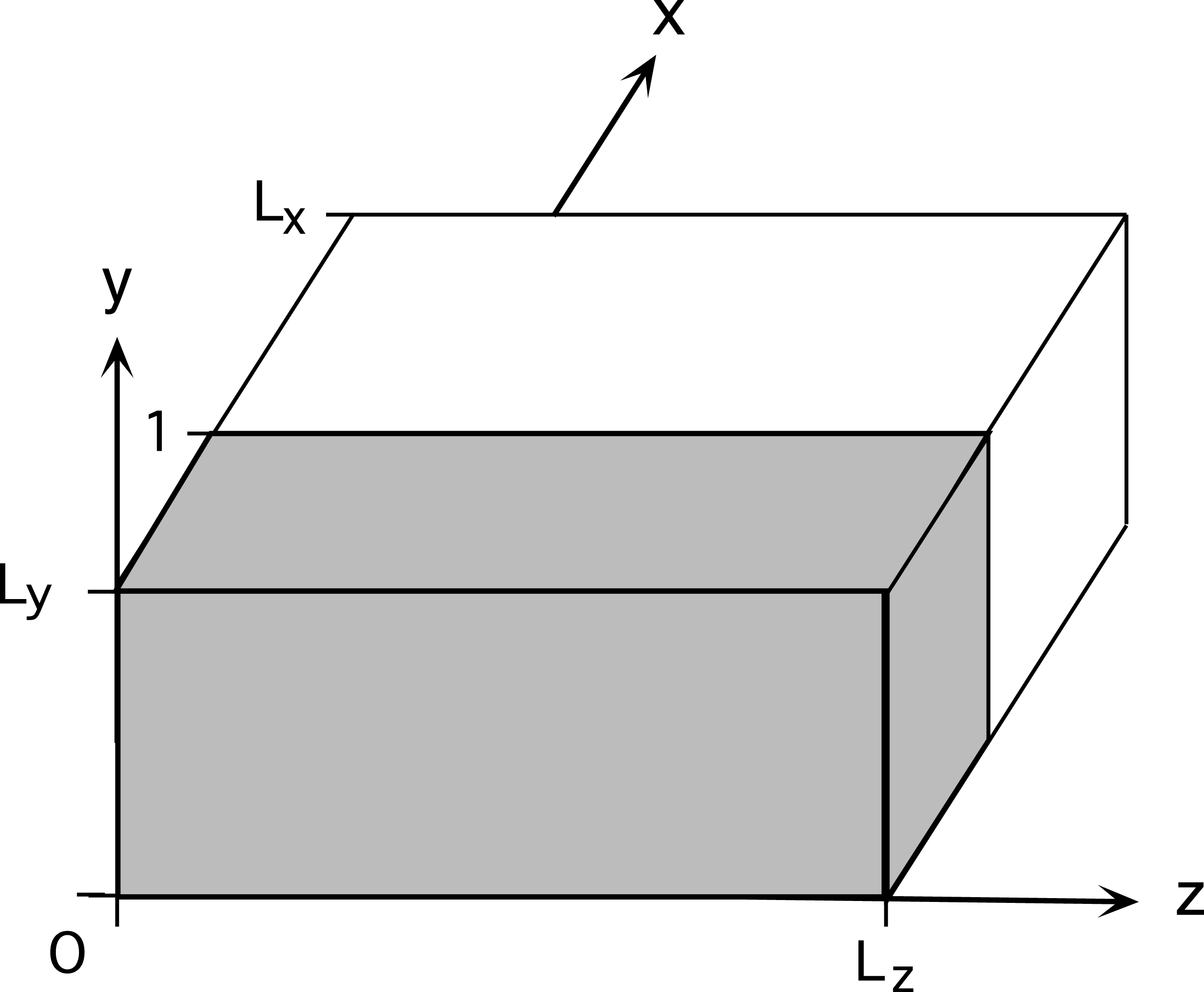
Figure 1 Long description
The diagram illustrates the schematic geometry of a dielectric slab or coronal flux tube that is infinitely extended in all directions. The phase velocity varies inside the slab, possibly with a jump at a specific point, and is constant elsewhere, equal to the velocity of light in vacuum. In the y-direction, the waves are imposed to be symmetric (even) or anti-symmetric (odd) with respect to the plane at y equals 1. Extensions along the negative directions are suppressed. All lengths are made dimensionless in units of the semi-thickness of the slab. The diagram includes axes labeled x, y, and z, with specific points and lengths marked, such as Lx, Ly, and Lz.
2. Electrodynamic waves in a dielectric slab
2.1. Basic equations
We exploit Maxwell’s equations in the absence of currents and space charges, where one-dimensional inhomogeneity occurs through the dielectric constant, which is not constant though in the dielectric slab, $\epsilon = \epsilon (x)$
for
$\epsilon = \epsilon (x)$
for $|x| \leqslant 1$
(see figure 1). In this figure, the coordinate
$|x| \leqslant 1$
(see figure 1). In this figure, the coordinate $x$
has already been scaled as indicated in (2.1). Outside the slab, we make the rather accurate approximation (even for air) that the magnetic permeability
$x$
has already been scaled as indicated in (2.1). Outside the slab, we make the rather accurate approximation (even for air) that the magnetic permeability $\mu _0$
and the dielectric constant
$\mu _0$
and the dielectric constant $\epsilon _0$
have their vacuum values,
$\epsilon _0$
have their vacuum values, $(\epsilon _0\mu _0)^{-1/2} = c$
. This permits us to eliminate these constants of nature by transforming to natural units, where all space and time variables and, hence, also the phase velocity of the electromagnetic waves, become dimensionless and of the order unity:
$(\epsilon _0\mu _0)^{-1/2} = c$
. This permits us to eliminate these constants of nature by transforming to natural units, where all space and time variables and, hence, also the phase velocity of the electromagnetic waves, become dimensionless and of the order unity:
 \begin{equation} x/a \rightarrow x ,\qquad t(c/a) \rightarrow t , \qquad v/c \rightarrow v , \end{equation}
with similar expressions for the other spatial directions. Hence, for our analysis, the only function of interest is the phase velocity, related to the index of refraction, $v(x) = 1/n(x)$
, both of which only deviate from unity in the dielectric slab:
$v(x) = 1/n(x)$
, both of which only deviate from unity in the dielectric slab:
 \begin{equation} v(x) \left \{ \begin{array}{l} \leqslant 1, \\[5pt] = 1, \end{array} \right .\quad n(x) \left \{ \begin{array}{l} \geqslant 1 \; {(\mathrm{inside\ the\ slab},\ |x| \leqslant 1),} \\ = 1 \; {(\mathrm{outside\ the\ slab},\ |x| \gt 1).} \end{array} \right . \end{equation}
The explicit functional dependence for $v(x)$
will be chosen in § 3.1 when the eigenvalue spectra of the waves are calculated. Notice that the dielectric is assumed to be non-magnetic and also non-dispersive, i.e. the phase velocity does not depend on the frequency of the waves.
$v(x)$
will be chosen in § 3.1 when the eigenvalue spectra of the waves are calculated. Notice that the dielectric is assumed to be non-magnetic and also non-dispersive, i.e. the phase velocity does not depend on the frequency of the waves.
In natural units, $\mathbf{D} \equiv \mathbf{E}/v^2$
and
$\mathbf{D} \equiv \mathbf{E}/v^2$
and $\mathbf{B} \equiv \mathbf{H}$
, so that
$\mathbf{B} \equiv \mathbf{H}$
, so that $\mathbf{E}$
and
$\mathbf{E}$
and $\mathbf{H}$
become the basic electrodynamic variables satisfying Maxwell’s equations in the absence of currents and space charges:
$\mathbf{H}$
become the basic electrodynamic variables satisfying Maxwell’s equations in the absence of currents and space charges:
 \begin{equation} \frac {1}{v^2}\frac {\partial \mathbf{E}}{\partial t} = \boldsymbol{\nabla }\times \mathbf{H} ,\quad \boldsymbol{\nabla }\boldsymbol{\cdot }{(\mathbf{E}/v^2)} = 0 ,\qquad \frac {\partial \mathbf{H}}{\partial t} = - \boldsymbol{\nabla }\times \mathbf{E} ,\quad \boldsymbol{\nabla }\boldsymbol{\cdot }{\mathbf{H}} = 0 . \end{equation}
For harmonic time dependence $\exp {(-{\mathrm{i}}\omega t})$
, they may be written in terms of the electric field alone,
$\exp {(-{\mathrm{i}}\omega t})$
, they may be written in terms of the electric field alone,
 \begin{equation} \frac {1}{v^2}\frac {\partial ^2 \mathbf{E}}{\partial t^2} + \boldsymbol{\nabla }\times \boldsymbol{\nabla }\times \mathbf{E} = 0 \quad \Rightarrow \quad ({\omega ^2}/v^2){\mathbf{E}} - \boldsymbol{\nabla }\times \boldsymbol{\nabla }\times \mathbf{E} = 0. \end{equation}
Since $\boldsymbol{\nabla }\boldsymbol{\cdot }{(\mathbf{E}/v^2)}$
vanishes everywhere, one component of the electric field may be eliminated. In this representation, the evolution of the magnetic field is just a consequence of the dynamics of the electric field:
$\boldsymbol{\nabla }\boldsymbol{\cdot }{(\mathbf{E}/v^2)}$
vanishes everywhere, one component of the electric field may be eliminated. In this representation, the evolution of the magnetic field is just a consequence of the dynamics of the electric field:
 \begin{equation} \frac {\partial \mathbf{H}}{\partial t} = - \boldsymbol{\nabla }\times \mathbf{E} \quad \Rightarrow \quad {\mathbf{H}} = - (\mathrm{i}/\omega )\boldsymbol{\nabla }\times \mathbf{E}. \end{equation}
Hence, the problem has been reduced to solving the basic differential equation (2.4) for two components of $\mathbf{E}$
, whereas the remaining component and the three components of
$\mathbf{E}$
, whereas the remaining component and the three components of $\mathbf{H}$
follow by algebraic expressions. Of course, one could also depart from the analogous equations for the magnetic field variable
$\mathbf{H}$
follow by algebraic expressions. Of course, one could also depart from the analogous equations for the magnetic field variable $\mathbf{H}$
, so that the electric field variable would become secondary. Notice though that the differential equations for
$\mathbf{H}$
, so that the electric field variable would become secondary. Notice though that the differential equations for $\mathbf{H}$
differ in their dependence on
$\mathbf{H}$
differ in their dependence on $v(x)$
from the differential equations for
$v(x)$
from the differential equations for $\mathbf{E}$
so that there is no symmetry between these variables in the dielectric.
$\mathbf{E}$
so that there is no symmetry between these variables in the dielectric.
2.2. Ordinary differential equations for electrodynamic waves
The one-dimensional configuration depicted in figure 1 admits a representation of the components of $\mathbf{E}$
and
$\mathbf{E}$
and $\mathbf{H}$
in terms of normal modes of the form
$\mathbf{H}$
in terms of normal modes of the form
 \begin{equation} f(x){\mathrm{e}}^{\mathrm{i}(\ell y + k z - \omega t)} , \end{equation}
where the functional dependence on the coordinate $x$
is to be determined by the solution of the ordinary differential equations (ODEs) corresponding to (2.4). The mode number
$x$
is to be determined by the solution of the ordinary differential equations (ODEs) corresponding to (2.4). The mode number $\ell$
in the vertical direction will be dropped right away since a rotation about the
$\ell$
in the vertical direction will be dropped right away since a rotation about the $x$
-axis produces a coordinate frame with
$x$
-axis produces a coordinate frame with $\ell = 0$
. It is here introduced for the sake of comparison with the MHD problem, where this symmetry is not present. Also, in the dielectric problem for the more relevant cylindrical configuration, the translational symmetry in
$\ell = 0$
. It is here introduced for the sake of comparison with the MHD problem, where this symmetry is not present. Also, in the dielectric problem for the more relevant cylindrical configuration, the translational symmetry in $y$
is to be replaced by the rotational symmetry in the angle
$y$
is to be replaced by the rotational symmetry in the angle $\theta$
with the corresponding mode number
$\theta$
with the corresponding mode number $m$
, which also cannot be transformed away. Without the mode number
$m$
, which also cannot be transformed away. Without the mode number $\ell$
, the ODE (2.4) becomes
$\ell$
, the ODE (2.4) becomes
 \begin{equation} \left (\begin{array}{@{}c@{\quad}c@{\quad}c@{}} \omega ^2/v^2 - k^2 & 0 & - {\mathrm{i}} k \partial _x \\[4pt] 0 & \partial _x^2 + \omega ^2/v^2 - k^2 & 0 \\[4pt] - {\mathrm{i}} k \partial _x & 0 &\partial _x^2 + \omega ^2/v^2 \end{array} \right ) \left (\begin{array}{@{}c} E_x \\[4pt] E_y \\[4pt] E_z \end{array} \right ) = 0 , \end{equation}
whereas (2.3b ) allows to eliminate one of the components of the electric field,
 \begin{equation} (E_x/v^2)^{\prime} + {\mathrm{i}} k E_z/v^2 = 0 , \end{equation}
and (2.5) gives the expressions for the magnetic field in terms of the electric field solutions of the ODEs (2.7),
 \begin{equation} H_x = - (k/\omega ) E_y , \quad H_y = (k/\omega ) E_x + ({\mathrm{i}}/\omega ) E_z^{\prime} , \quad H_z = - ({\mathrm{i}}/\omega ) E_y^{\prime} . \end{equation}
Equations (2.7)–(2.9) determine the solutions of this one-dimensional problem.
An obvious solution is seen at once, viz. the TE mode with $E_x = E_z = 0$
,
$E_x = E_z = 0$
, $H_y = 0$
, and is described by the second-order ODE for the transverse (with respect to the propagation direction of the waves) component of the electric field,
$H_y = 0$
, and is described by the second-order ODE for the transverse (with respect to the propagation direction of the waves) component of the electric field,
 \begin{equation} \frac {\displaystyle {{\rm d}^2}E_y}{\displaystyle {\rm d}{x^2}} + (\omega ^2/v^2 - k^2) E_y = 0 , \end{equation}
or by the equivalent system of first order ODEs,
 \begin{equation} \left \{\begin{array}{@{}l@{}l} \frac {\displaystyle {\rm d} E_y}{\displaystyle {\rm d}x} - {\mathrm{i}} \omega H_z = 0 , \\[10pt] \frac {\displaystyle {\rm d} H_z}{\displaystyle {\rm d}x} - ({\mathrm{i}}/\omega ) (\omega ^2/v^2 - k^2) E_y = 0 , \end{array} \right .\end{equation}
whereas $ H_x = - (k/\omega ) E_y$
is just an algebraic consequence. The other solution, for the TM mode with
$ H_x = - (k/\omega ) E_y$
is just an algebraic consequence. The other solution, for the TM mode with $H_x = H_z = 0$
,
$H_x = H_z = 0$
, $E_y = 0$
, is described by an analogous second-order ODE for the transverse component
$E_y = 0$
, is described by an analogous second-order ODE for the transverse component $B_y$
of the magnetic field (or the equivalent system of first-order ODEs in terms of
$B_y$
of the magnetic field (or the equivalent system of first-order ODEs in terms of $H_y$
and
$H_y$
and $E_z$
), whereas the expression for
$E_z$
), whereas the expression for $E_x$
is just an algebraic consequence. These equations are more conveniently obtained from the mirror images of (2.4)–(2.5) where the roles of
$E_x$
is just an algebraic consequence. These equations are more conveniently obtained from the mirror images of (2.4)–(2.5) where the roles of $\mathbf{E}$
and
$\mathbf{E}$
and $\mathbf{H}$
are exchanged, albeit with different dependencies on
$\mathbf{H}$
are exchanged, albeit with different dependencies on $v(x)$
. As a result, the spectrum of the TM modes differs slightly from the spectrum of the TE modes. We will restrict the analysis to the TE modes, but it is obvious that analogous results would be obtained for the TM modes. In conclusion, the full electromagnetic spectral wave problem is described by two second-order ODEs for two slightly different modes, whereas the full MHD spectral wave problem (discussed in § 5) is described by only one second-order ODE, but for three completely different modes (slow magneto-sonic, Alfvén and fast magneto-sonic) with three different phase velocities. Also notice that for real
$v(x)$
. As a result, the spectrum of the TM modes differs slightly from the spectrum of the TE modes. We will restrict the analysis to the TE modes, but it is obvious that analogous results would be obtained for the TM modes. In conclusion, the full electromagnetic spectral wave problem is described by two second-order ODEs for two slightly different modes, whereas the full MHD spectral wave problem (discussed in § 5) is described by only one second-order ODE, but for three completely different modes (slow magneto-sonic, Alfvén and fast magneto-sonic) with three different phase velocities. Also notice that for real $\omega ^2$
, the spectral equation (2.10) is of the standard Sturm–Liouville type with monotonicity of the eigenvalues with the number of nodes of the internal part of the eigenfunctions, whereas the corresponding MHD equation is much more complicated. Of course, calling (2.10) a second-order ODE and (2.11) first-order ODEs is only loosely speaking since, for the numerical computation of the complex leaky mode spectra, the number of ODEs actually should be multiplied by two for the real and imaginary components of the eigenfunctions involved. Those components will be distinguished by the subscripts
$\omega ^2$
, the spectral equation (2.10) is of the standard Sturm–Liouville type with monotonicity of the eigenvalues with the number of nodes of the internal part of the eigenfunctions, whereas the corresponding MHD equation is much more complicated. Of course, calling (2.10) a second-order ODE and (2.11) first-order ODEs is only loosely speaking since, for the numerical computation of the complex leaky mode spectra, the number of ODEs actually should be multiplied by two for the real and imaginary components of the eigenfunctions involved. Those components will be distinguished by the subscripts $1$
and
$1$
and $2$
.
$2$
.
2.3. Boundary value problem for TE modes
Since the TE modes are fully described by the electric field component $E_y$
, with the auxiliary magnetic field component
$E_y$
, with the auxiliary magnetic field component $H_z$
, it is convenient for the algebra to simply write
$H_z$
, it is convenient for the algebra to simply write $E \equiv E_y$
and
$E \equiv E_y$
and $H \equiv H_z$
, and to distinguish the outside variables from the inside ones by a hat,
$H \equiv H_z$
, and to distinguish the outside variables from the inside ones by a hat, $\hat {E}$
and
$\hat {E}$
and $\hat {H}$
. With the prescription (2.2) of the phase velocity
$\hat {H}$
. With the prescription (2.2) of the phase velocity $v(x)$
, the spectral equation (2.10) is valid everywhere. Dropping the exponential factor
$v(x)$
, the spectral equation (2.10) is valid everywhere. Dropping the exponential factor $\exp {\mathrm{i}}(k z - \omega t)$
, the internal solution is then written as
$\exp {\mathrm{i}}(k z - \omega t)$
, the internal solution is then written as
 \begin{equation} E = E(x) ,\quad H = H(x) = - ({\mathrm{i}}/\omega ) E^{\prime}(x) \qquad (|x| \leqslant 1) . \end{equation}
Since $v(x)$
is assumed to be arbitrary inside the slab, these expressions are to be determined numerically. Outside the slab,
$v(x)$
is assumed to be arbitrary inside the slab, these expressions are to be determined numerically. Outside the slab, $v(x) = 1$
, and the external solution is trivial:
$v(x) = 1$
, and the external solution is trivial:
 \begin{equation} \hat {E}(x) = \hat {\alpha }{\mathrm{e}}^{{\mathrm{i}}\hat {q}x} + \hat {\beta }{\mathrm{e}}^{-{\mathrm{i}} \hat {q}x} ,\quad \hat {H}(x) = (\hat {q}/\omega ) (\hat {\alpha }{\mathrm{e}}^{{\mathrm{i}}\hat {q}x} - \hat {\beta }{\mathrm{e}}^{-{\mathrm{i}} \hat {q}x}) \qquad (|x| \gt 1) . \end{equation}
If $v(x)$
is assumed to be constant inside the slab, the internal solution also becomes trivial, of the same form as (2.13) without the hats, and the standard solutions for leaky modes (Huang et al. Reference Huang, Xu, Powell, Padilla and Miroshnichenko2023) are obtained. In that case,
$v(x)$
is assumed to be constant inside the slab, the internal solution also becomes trivial, of the same form as (2.13) without the hats, and the standard solutions for leaky modes (Huang et al. Reference Huang, Xu, Powell, Padilla and Miroshnichenko2023) are obtained. In that case, $\beta = \pm \alpha$
and
$\beta = \pm \alpha$
and $\hat {\beta } = 0$
, and the jump of the phase velocity at
$\hat {\beta } = 0$
, and the jump of the phase velocity at $|x| = 1$
produces the final dispersion equation. However, such an assumption is unduly restrictive since problems of genuine interest do not permit this simplification. Also, in the corresponding MHD problem, this would brush the central Alfvén singularity under the carpet. Actually, the main problem to be solved here is not the solution of differential equations (excellent and accurate numerical techniques exist for this purpose), but the satisfaction of the associated boundary conditions (BCs), i.e. the solution of the eigenvalue problem.
$|x| = 1$
produces the final dispersion equation. However, such an assumption is unduly restrictive since problems of genuine interest do not permit this simplification. Also, in the corresponding MHD problem, this would brush the central Alfvén singularity under the carpet. Actually, the main problem to be solved here is not the solution of differential equations (excellent and accurate numerical techniques exist for this purpose), but the satisfaction of the associated boundary conditions (BCs), i.e. the solution of the eigenvalue problem.
For that solution, the complex eigenvalue $\omega \equiv \sigma + {\mathrm{i}}\nu$
and the real longitudinal wave number
$\omega \equiv \sigma + {\mathrm{i}}\nu$
and the real longitudinal wave number $k$
will be treated as known parameters, so that the real and imaginary parts of the complex transverse wavenumber
$k$
will be treated as known parameters, so that the real and imaginary parts of the complex transverse wavenumber $\hat {q}\equiv \hat {q}_1 + {\mathrm{i}}\hat{q}_2$
are to be found from the inverse external dispersion equation:
$\hat {q}\equiv \hat {q}_1 + {\mathrm{i}}\hat{q}_2$
are to be found from the inverse external dispersion equation:
 \begin{align} {\omega ^2} &= \hat {q}^2 + k^2 \quad \Rightarrow \quad \hat {q} = \pm \sqrt {{\omega ^2} - k^2} = \pm A {\mathrm{e}}^{{\mathrm{i}}\varphi } , \nonumber\\[4pt]&A \equiv (u^2 + v^2)^{1/4},\quad \varphi \equiv {\frac {1}{2}} \arctan (v/u) ,\qquad u \equiv \sigma ^2 - \nu ^2 - k^2 ,\quad v \equiv 2 \sigma \nu . \end{align}
The central BC, given in (2.24), matching the numerical internal solution $\{E(x), H(x)\}$
to the explicit external solution
$\{E(x), H(x)\}$
to the explicit external solution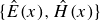 $\{\hat {E}(x), \hat {H}(x)\}$
at
$\{\hat {E}(x), \hat {H}(x)\}$
at $x = 1$
, implies matching something like the ‘internal wavenumber’
$x = 1$
, implies matching something like the ‘internal wavenumber’ $q$
to the external wavenumber
$q$
to the external wavenumber $\hat {q}$
. For constant phase velocity, that internal wavenumber
$\hat {q}$
. For constant phase velocity, that internal wavenumber $q$
would follow from the internal dispersion equation
$q$
would follow from the internal dispersion equation ${\omega ^2} = (q^2 + k^2) v^2$
. Here, it simply will be an implicit property of the internal solution
${\omega ^2} = (q^2 + k^2) v^2$
. Here, it simply will be an implicit property of the internal solution $\{E(x),B(x)\}$
of the ODEs (2.11) which gradually transform the wavelengths due to the variation of
$\{E(x),B(x)\}$
of the ODEs (2.11) which gradually transform the wavelengths due to the variation of $v(x)$
. Through the definitions (2.14) for
$v(x)$
. Through the definitions (2.14) for $A$
,
$A$
, $\varphi$
,
$\varphi$
, $u$
and
$u$
and $v$
, the expressions for
$v$
, the expressions for $\hat {q}_1$
and
$\hat {q}_1$
and $\hat {q}_2$
will be different for the different parts of the complex
$\hat {q}_2$
will be different for the different parts of the complex $\omega$
-plane separated by the lines
$\omega$
-plane separated by the lines $\sigma = 0$
,
$\sigma = 0$
, $\nu = 0$
, and the hyperbola
$\nu = 0$
, and the hyperbola $\sigma ^2 -\nu ^2 = k^2$
(see figure 2). In particular, the choice of the
$\sigma ^2 -\nu ^2 = k^2$
(see figure 2). In particular, the choice of the $\pm$
sign is dictated by the fact that we wish to associate the coefficient
$\pm$
sign is dictated by the fact that we wish to associate the coefficient $\hat {\alpha }$
with outgoing waves and the coefficient
$\hat {\alpha }$
with outgoing waves and the coefficient $\hat {\beta }$
with ingoing waves. It is indicated in the figure for the different areas of the complex
$\hat {\beta }$
with ingoing waves. It is indicated in the figure for the different areas of the complex $\omega$
-plane:
$\omega$
-plane:
Complex $\omega$
-plane divided by the hyperbola
$\omega$
-plane divided by the hyperbola $u = 0$
, i.e
$u = 0$
, i.e $\sigma ^2 - \nu ^2 = k^2$
, and the lines
$\sigma ^2 - \nu ^2 = k^2$
, and the lines $v = 0$
, i.e
$v = 0$
, i.e $\sigma = 0$
and
$\sigma = 0$
and $\nu = 0$
, in eight regions with the indicated choice of the
$\nu = 0$
, in eight regions with the indicated choice of the $\pm$
sign in the expression (2.14) for the external wavenumber
$\pm$
sign in the expression (2.14) for the external wavenumber $\hat {q}$
.
$\hat {q}$
.
– for region ${\unicode{x2460}}\,,\, u \leqslant 0 ,\, \nu \leqslant 0 \,$
:
$- {\frac {1}{2}} \pi \leqslant \varphi \lt - {\frac {1}{4}} \pi \quad \Rightarrow \quad \hat {q}_1 \geqslant 0 , \, \hat {q}_2 \lt 0\,$
;
${\unicode{x2460}}\,,\, u \leqslant 0 ,\, \nu \leqslant 0 \,$
:
$- {\frac {1}{2}} \pi \leqslant \varphi \lt - {\frac {1}{4}} \pi \quad \Rightarrow \quad \hat {q}_1 \geqslant 0 , \, \hat {q}_2 \lt 0\,$
;– for region
${\unicode{x2461}}\,,\, u \gt 0 ,\, \nu \leqslant 0 \,$
:
$- {\frac {1}{4}} \pi \lt \varphi \leqslant 0 \quad \qquad\!\! \Rightarrow \quad \hat {q}_1 \gt 0 , \, \hat {q}_2 \leqslant 0\,$
;– for region
${\unicode{x2462}}\,,\, u \gt 0 ,\, \nu \gt 0 \,$
:
$\quad 0 \lt \varphi \lt {\frac {1}{4}} \pi \qquad\!\! \Rightarrow \quad \hat {q}_1 \gt 0 , \, \hat {q}_2 \gt 0 \,$
;– for region
${\unicode{x2463}}\,,\, u \leqslant 0 ,\, \nu \gt 0 \,$
:
${\frac {1}{4}} \pi \leqslant \varphi \lt {\frac {1}{2}} \pi \qquad\!\! \Rightarrow \quad \hat {q}_1 \lt 0 , \, \hat {q}_2 \lt 0\,$
.








The sign changes across the real axis are crucial to compute the Spectral Webs of figure 4.
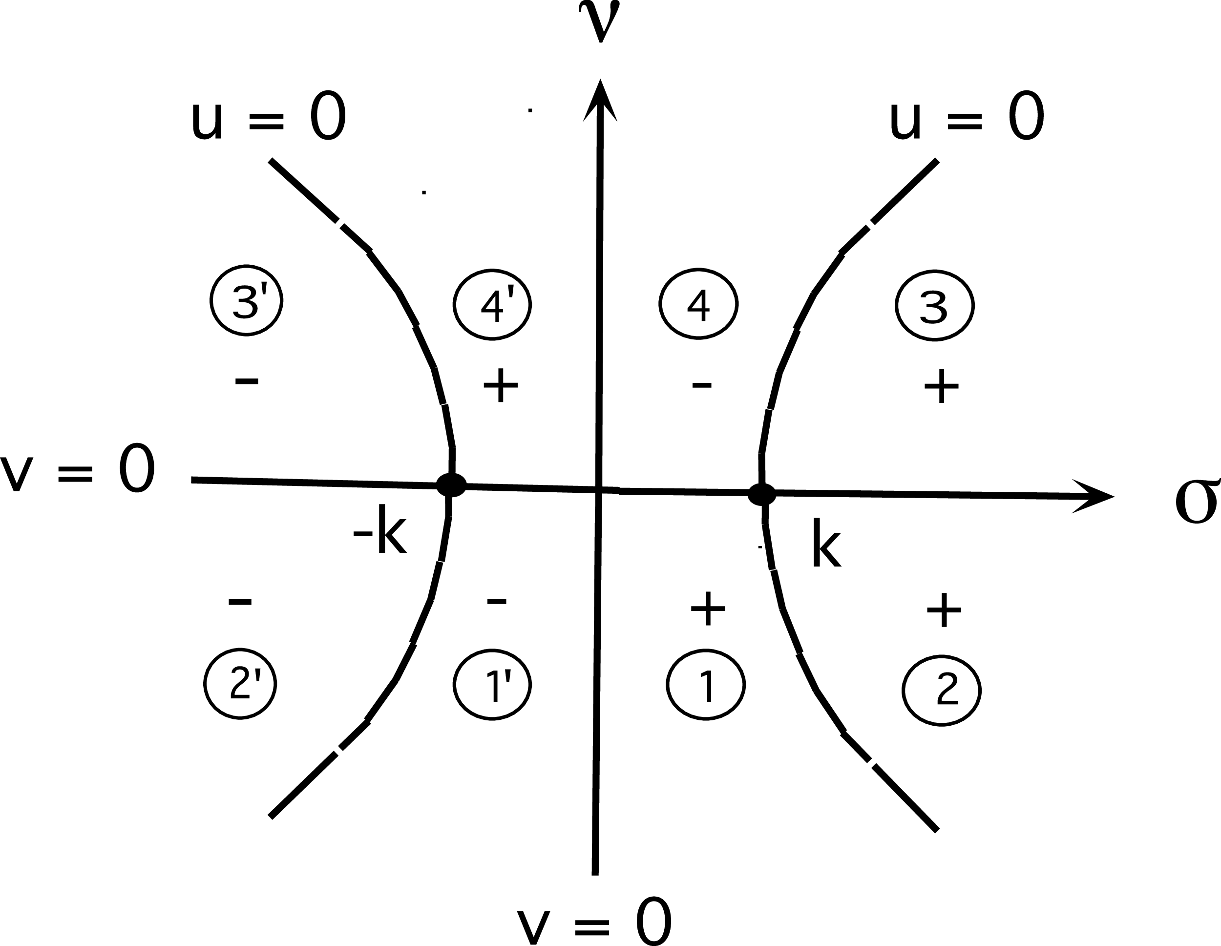
Figure 2 Long description
The complex plane is divided by the hyperbola u equals zero and the lines v equals zero and sigma equals plus minus k, creating eight regions. Each region is labeled with a number and has an indicated sign for the external wavenumber. Region 1 has a positive sign, region 2 has a positive sign, region 3 has a positive sign, region 4 has a negative sign, region 1 prime has a negative sign, region 2 prime has a negative sign, region 3 prime has a negative sign, and region 4 prime has a positive sign. The sign changes across the real axis are crucial for computing the Spectral Webs.
To exhibit the propagation properties of the waves associated with $\hat {\alpha }$
and
$\hat {\alpha }$
and $\hat {\beta }$
, it is expedient to restore the time dependence, and to split real and imaginary parts of the exponential factors of the external solutions:
$\hat {\beta }$
, it is expedient to restore the time dependence, and to split real and imaginary parts of the exponential factors of the external solutions:
 \begin{equation} \hat {E}(x,t) = \hat {\alpha }{\mathrm{e}}^{-\hat {q}_2 x + \nu t}{\mathrm{e}}^{{\mathrm{i}}(\hat {q}_1 x - \sigma t)} + \hat {\beta }{\mathrm{e}}^{\hat{q}_2 x + \nu t}{\mathrm{e}}^{- {\mathrm{i}}(\hat {q}_1 x + \sigma t)} , \end{equation}
and similarly for $\hat {H}(x,t)$
. For positive values of
$\hat {H}(x,t)$
. For positive values of $\hat {q}_1$
and
$\hat {q}_1$
and $\sigma$
, the factor
$\sigma$
, the factor $\hat {\alpha }$
then corresponds to the outwardly propagating part of the waves and the factor
$\hat {\alpha }$
then corresponds to the outwardly propagating part of the waves and the factor $\hat {\beta }$
corresponds to the inwardly propagating part. We may restrict the computation of the solutions to
$\hat {\beta }$
corresponds to the inwardly propagating part. We may restrict the computation of the solutions to $x \geqslant 0$
since the complete functions, including the behaviour for
$x \geqslant 0$
since the complete functions, including the behaviour for $x \lt 0$
, simply follows from the symmetry imposed at the origin, expressed by the BCs (2.23). For leaky modes propagating exclusively in the
$x \lt 0$
, simply follows from the symmetry imposed at the origin, expressed by the BCs (2.23). For leaky modes propagating exclusively in the $x$
-direction (
$x$
-direction ( $k = 0$
), as in Huang et al. (Reference Huang, Xu, Powell, Padilla and Miroshnichenko2023) and our previous paper (Goedbloed et al. Reference Goedbloed, Keppens and Poedts2023), the relation between
$k = 0$
), as in Huang et al. (Reference Huang, Xu, Powell, Padilla and Miroshnichenko2023) and our previous paper (Goedbloed et al. Reference Goedbloed, Keppens and Poedts2023), the relation between $\hat {q}$
and
$\hat {q}$
and $\omega$
is obvious:
$\omega$
is obvious: $\hat {q}_1 = \sigma$
and
$\hat {q}_1 = \sigma$
and $\hat {q}_2 = \nu$
. In that case, the outward part (with
$\hat {q}_2 = \nu$
. In that case, the outward part (with $\hat {\alpha }$
) is exponentially growing in space for
$\hat {\alpha }$
) is exponentially growing in space for $x \rightarrow \infty$
and exponentially damped in time for
$x \rightarrow \infty$
and exponentially damped in time for $t \rightarrow \infty$
, and for the inward part (with
$t \rightarrow \infty$
, and for the inward part (with $\hat {\beta }$
), this behaviour occurs for negative values of
$\hat {\beta }$
), this behaviour occurs for negative values of $x$
and
$x$
and $t$
. Assuming an open boundary at
$t$
. Assuming an open boundary at $x = L_x \rightarrow \infty$
which does not reflect waves, it is natural to impose the condition
$x = L_x \rightarrow \infty$
which does not reflect waves, it is natural to impose the condition $\hat {\beta } = 0$
. This implies that the external solution behaves as
$\hat {\beta } = 0$
. This implies that the external solution behaves as $\hat {\alpha } \exp (-\hat {q}_2 x)$
, so that it explodes at infinity for
$\hat {\alpha } \exp (-\hat {q}_2 x)$
, so that it explodes at infinity for $\hat {q}_2 \lt 0$
, which is the characteristic feature of leaky modes. This infinity, the reason for concern about the physics of these modes, will be discussed in § 4.
$\hat {q}_2 \lt 0$
, which is the characteristic feature of leaky modes. This infinity, the reason for concern about the physics of these modes, will be discussed in § 4.
For conservative waves, with real frequencies, propagating in the $z$
-direction (
$z$
-direction ( $k \ne 0$
), infinities for
$k \ne 0$
), infinities for $x \rightarrow \infty$
are avoided, even with an open boundary, since
$x \rightarrow \infty$
are avoided, even with an open boundary, since $\nu = 0$
and the values of
$\nu = 0$
and the values of $\hat {q}$
are then restricted by another condition. In that case, the square root sign in the inverse dispersion equation (2.14) gives rise to the following distinction of the propagation properties of the external waves:
$\hat {q}$
are then restricted by another condition. In that case, the square root sign in the inverse dispersion equation (2.14) gives rise to the following distinction of the propagation properties of the external waves:
 \begin{equation} \hat {q} = \hat {q}_1 + {\mathrm{i}}\hat {q}_2 ,\ \left \{\begin{array}{l@{\quad}l} \hat {q}_1 = 0 ,\quad \hat {q}_2 = - \sqrt {k^2 - \sigma ^2} &\quad {(\text{for } |\sigma | \lt k\!:\, \text{evanescense})} , \\[3mm] \hat {q}_1 = \sqrt {\sigma ^2 - k^2} ,\quad \hat {q}_2 = 0 &\quad {(\text{for }|\sigma | \geqslant k\!:\, \text{propagation})} . \end{array} \right . \end{equation}
Evanescence in the external region ( $|x| \geqslant 1$
) does not imply evanescence in the internal region: a discrete spectrum of so-called bound modes may be found there, see Snyder & Love (Reference Snyder and Love1983, p. 206). The first expression is also valid for the leaky modes in the
$|x| \geqslant 1$
) does not imply evanescence in the internal region: a discrete spectrum of so-called bound modes may be found there, see Snyder & Love (Reference Snyder and Love1983, p. 206). The first expression is also valid for the leaky modes in the $u \lt 0$
part of the
$u \lt 0$
part of the $\omega$
-plane, i.e. in the so-called cutoff regions
$\omega$
-plane, i.e. in the so-called cutoff regions $1$
,
$1$
, $4$
(and
$4$
(and $1^{\prime}$
,
$1^{\prime}$
, $4^{\prime}$
) of figure 2. However, the external part of the waves is then explosively growing. It should be noticed also that the description ‘propagative’, while appropriate for leaky modes, is actually a misnomer for the conservative modes since these modes are standing waves that do not propagate at all, as we will see shortly.
$4^{\prime}$
) of figure 2. However, the external part of the waves is then explosively growing. It should be noticed also that the description ‘propagative’, while appropriate for leaky modes, is actually a misnomer for the conservative modes since these modes are standing waves that do not propagate at all, as we will see shortly.
To characterise the different cases and to obtain the pertinent external BCs, we construct the flow of electromagnetic energy, i.e. the Poynting flux, for $|x| \gt 1$
:
$|x| \gt 1$
:
 \begin{equation} \hat {\mathbf{S}} \equiv \hat {\mathbf{E}} \times \hat {\mathbf{H}}^* = \hat {E}(x) \hat {H}^*(x) \mathbf{e}_x + (k/\omega ^*) \hat {E}(x) \hat {E}^*(x) \mathbf{e}_z . \end{equation}
Because the system is homogeneous in the $z$
-direction, the contribution of
$z$
-direction, the contribution of $\hat {S}_z$
just represents a constant flow of energy in that direction, which is of no interest for the present boundary value problem (BVP). Hence, to study the external solutions, the expression for the Poynting flux may be restricted to the
$\hat {S}_z$
just represents a constant flow of energy in that direction, which is of no interest for the present boundary value problem (BVP). Hence, to study the external solutions, the expression for the Poynting flux may be restricted to the $x$
-component:
$x$
-component:
 \begin{equation} \hat {S}_x(x) = (\hat {q}^*/\omega ^*) \big[|\hat {\alpha }|^2 {\mathrm{e}}^{- 2\hat {q}_2 x} - |\hat {\beta }|^2 {\mathrm{e}}^{2\hat {q}_2 x} - \hat {\alpha } \hat {\beta }^* {\mathrm{e}}^{2{\mathrm{i}}\hat {q}_1 x} + \hat {\alpha }^* \hat {\beta } {\mathrm{e}}^{-2 {\mathrm{i}}\hat {q}_1 x} \big] , \end{equation}
where the choice of $\hat {\alpha }_{1,2}$
and
$\hat {\alpha }_{1,2}$
and $\hat {\beta }_{1,2}$
represents different physical problems. This implies
$\hat {\beta }_{1,2}$
represents different physical problems. This implies
– for conservative bound modes (real, $|\sigma | \lt k$
,
$|\sigma | \lt k$
, $\hat {q}_1 = 0$
):
$\hat {q}_1 = 0$
):
 \begin{equation} \hat {\alpha } = 0 \ \Rightarrow \ {\mathrm{Re}}(\hat {S}_x) = 0 ,\quad {\mathrm{Im}}(\hat {S}_x) = (\hat {q}_2/\sigma ) |\hat {\beta }|^2{\mathrm{e}}^{2\hat {q}_2 x}|_{x \rightarrow \infty } \rightarrow 0 , \end{equation}
– for conservative ‘propagating’ modes (real, $|\sigma | \geqslant k$
,
$|\sigma | \geqslant k$
, $\hat {q}_2 = 0$
):
$\hat {q}_2 = 0$
):
 \begin{align} \hat {\alpha } = \hat {\beta }{\mathrm{e}}^{-2{\mathrm{i}}\varphi } \ \Rightarrow \ {\mathrm{Re}}(\hat {S}_x) = 0 , \quad {\mathrm{Im}}(\hat {S}_x) = - 2 (\hat {q}_1/\sigma ) |\hat {\beta }|^2\sin 2(\hat {q}_1 x -\varphi )|_{\mathrm{finite \,all \,x}},\nonumber\\[-10pt]\nonumber\\ \end{align}
– for cutoff leaky modes (most real, $|\sigma | \lt k$
, but some imaginary,
$|\sigma | \lt k$
, but some imaginary, $|\nu | \lt k$
,
$|\nu | \lt k$
, $\hat {q}_1 = 0$
):
$\hat {q}_1 = 0$
):
 \begin{align} \hat {\beta } = 0 \ \Rightarrow \left \{\begin{array}{@{}l@{}l} \nu = 0: \,{\mathrm{Re}}(\hat {S}_x) = 0 , \quad {\mathrm{Im}}(\hat {S}_x) = - (\hat {q}_2/\sigma ) |\hat {\alpha }|^2{\mathrm{e}}^{-2\hat {q}_2 x}|_{x \rightarrow \infty } \rightarrow \infty ,\\[8pt] \sigma = 0: \,{\mathrm{Re}}(\hat {S}_x) = (\hat {q}_2/\nu ) |\hat {\alpha }|^2{\mathrm{e}}^{-2\hat {q}_2 x}|_{x \rightarrow \infty } \rightarrow \infty ,\quad {\mathrm{Im}}(\hat {S}_x) = 0 ,\end{array} \right . \end{align}
– for propagating leaky modes (complex, $\sqrt {\sigma ^2 - \nu ^2} \geqslant k$
,
$\sqrt {\sigma ^2 - \nu ^2} \geqslant k$
, $\hat {q}_1 \ne 0$
,
$\hat {q}_1 \ne 0$
, $\hat {q}_2 \ne 0$
):
$\hat {q}_2 \ne 0$
):
 \begin{equation} \hat {\beta } = 0 \ \Rightarrow \ \hat {S}_x = (\hat {q}^*/\omega ^*) |\hat {\alpha }|^2{\mathrm{e}}^{- 2\hat {q}_2 x} \Rightarrow {\mathrm{Re}}(\hat {S}_x)|_{x \rightarrow \infty }\ \mathrm{and}\ {\mathrm{Im}}(\hat {S}_x)|_{x \rightarrow \infty } \rightarrow \infty . \end{equation}
Consequently, the two kinds of modes may be distinguished by whether both components of $\hat {S}_x$
are finite (conservative modes) or at least one of them is unbounded (leaky modes). We will discuss in § 4 when and why the latter modes are still acceptable in a number of physical applications. For all cases with real eigenvalues,
$\hat {S}_x$
are finite (conservative modes) or at least one of them is unbounded (leaky modes). We will discuss in § 4 when and why the latter modes are still acceptable in a number of physical applications. For all cases with real eigenvalues, ${\mathrm{Re}}(\hat {S}_x) = 0$
for all
${\mathrm{Re}}(\hat {S}_x) = 0$
for all $|x| \gt 1$
, which represents the rate of energy change averaged over an oscillation period. Apparently, this condition does not distinguish conservative from leaky modes since a sub-spectrum of real discrete leaky modes also satisfies it according to (2.21). We will come back to this when discussing figure 4 in § 3.3.
$|x| \gt 1$
, which represents the rate of energy change averaged over an oscillation period. Apparently, this condition does not distinguish conservative from leaky modes since a sub-spectrum of real discrete leaky modes also satisfies it according to (2.21). We will come back to this when discussing figure 4 in § 3.3.
Summarising: the boundary value problems (BVPs) for the numerical solution of the spectral equation (2.10) imply imposing the following boundary conditions:
 \begin{align} \text{(a) at }|x| & = 0{:} \quad E(0) = 0 \; {(\mathrm{odd\ modes})} \quad \text{or}\quad H(0) = 0 \; (\mathrm{even\ modes}) ,\\[-10pt]\nonumber \end{align}
 \begin{align} \text{(b) at }|x| & = 1{:} \quad E(1) = \hat {E}(1) \quad \text{and}\quad H(1) = \hat {H}(1),\\[-10pt]\nonumber \end{align}
 \begin{align} \text{(c) at }|x| & \rightarrow \infty , \left \{\begin{array}{@{}l@{}l} (c1)\,\, \mathrm{CNMs}: \ \hat {\alpha } = 0 \ {(\text{for }\sigma ^2 - \nu ^2 \lt k^2)},\quad |\hat {\alpha }| = |\hat {\beta }| \\\qquad\qquad\qquad\qquad\qquad\qquad\qquad\qquad {(\text{for } \sigma ^2 - \nu ^2 \geqslant k^2)},\\[5pt] (c2)\,\, \mathrm{QNMs}: \ \hat {\beta } = 0. \end{array} \right . \end{align}
At this point, we have introduced our main focus with the split into the two distinct BVPs indicated by the labels (c1) for conservative normal modes (CNMs), with real eigenvalues, and (c2) for leaky, quasi-normal modes (QNMs), with real or complex eigenvalues. We exploit the acronym QNMs for the leaky modes following standard terminology, see e.g. Colom et al. (Reference Colom, McPhedran, Stout and Bonod2018) and Sauvan et al. (Reference Sauvan, Wu, Zarouf, Muljarov and Lalanne2022). The construction of the solutions of these BVPs involves matching the numerical internal solution $\{E(x), H(x)\}$
, determined by the BCs (2.23), to the explicit external solution
$\{E(x), H(x)\}$
, determined by the BCs (2.23), to the explicit external solution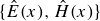 $\{\hat {E}(x), \hat {H}(x)\}$
, determined by the BCs (2.25), and subsequently trying to satisfy the two BCs (2.24). Satisfaction of the first one (on the electric field) can always be obtained by adapting the amplitude of the external part of the solution, but the second one (on the magnetic field) can only be satisfied for certain values of
$\{\hat {E}(x), \hat {H}(x)\}$
, determined by the BCs (2.25), and subsequently trying to satisfy the two BCs (2.24). Satisfaction of the first one (on the electric field) can always be obtained by adapting the amplitude of the external part of the solution, but the second one (on the magnetic field) can only be satisfied for certain values of $\omega$
, viz. the eigenvalues. Solution of this eigenvalue problem will be accomplished by means of the method of the Spectral Web, introduced in the following sub-section.
$\omega$
, viz. the eigenvalues. Solution of this eigenvalue problem will be accomplished by means of the method of the Spectral Web, introduced in the following sub-section.
Finally, it is to be noted that, by virtue of the explicit expressions (2.13) for the external solution, satisfaction of the BCs (2.25) for $|x| \rightarrow \infty$
directly transfers to explicit expressions for the variables
$|x| \rightarrow \infty$
directly transfers to explicit expressions for the variables $\hat {E}(1)$
and
$\hat {E}(1)$
and $\hat {H}(1)$
that are exploited in the Spectral Web method. Also, note that apostrophes have been put on ‘propagating’ for the real conservative modes in the region
$\hat {H}(1)$
that are exploited in the Spectral Web method. Also, note that apostrophes have been put on ‘propagating’ for the real conservative modes in the region $|\sigma | \geqslant k$
, with the property (2.20). That property guarantees perfect balance between the outgoing and ingoing waves so that these modes do not propagate at all! This implies that the appropriate terminology is standing conservative modes, distinguishing them from propagating leaky modes. This distinction is crucial for the different normalisations discussed in § 4.
$|\sigma | \geqslant k$
, with the property (2.20). That property guarantees perfect balance between the outgoing and ingoing waves so that these modes do not propagate at all! This implies that the appropriate terminology is standing conservative modes, distinguishing them from propagating leaky modes. This distinction is crucial for the different normalisations discussed in § 4.
2.4. Spectral Web for electrodynamic waves in dielectric media
Our method to construct the eigenvalue spectra is termed the Spectral Web, analogous to the Spectral Web for MHD plasmas introduced by Goedbloed (Reference Goedbloed2018) and effectively applied to accretion disks about black holes (Goedbloed & Keppens Reference Goedbloed and Keppens2022) discovering the new super-Alfvénic rotational instabilities (SARIs) described in that paper. Its counterpart is here developed for electrodynamic waves in dielectric media.
Satisfaction of the central BCs (2.24) for arbitrary complex values of $\omega$
implies that the four coefficients
$\omega$
implies that the four coefficients $\{\hat {\alpha }_{1,2}, \hat {\beta }_{1,2}\}$
of the external solution (2.13) are completely determined by the four boundary values
$\{\hat {\alpha }_{1,2}, \hat {\beta }_{1,2}\}$
of the external solution (2.13) are completely determined by the four boundary values $\{E_{1,2}(1), H_{1,2}(1)\}$
of the internal solutions (2.12):
$\{E_{1,2}(1), H_{1,2}(1)\}$
of the internal solutions (2.12):
 \begin{equation} \hat {\alpha } = {\frac {1}{2}} {\mathrm{e}}^{-{\mathrm{i}}\hat {q}} [E(1) + (\omega /\hat {q}) H(1)] ,\quad \hat {\beta } = {\frac {1}{2}} {\mathrm{e}}^{{\mathrm{i}}\hat {q}} [E(1) - (\omega /\hat {q}) H(1)]. \end{equation}
However, for arbitrary values of $\omega$
, this conflicts with also satisfying the outer BCs (2.25), since they involve a restriction on the coefficients
$\omega$
, this conflicts with also satisfying the outer BCs (2.25), since they involve a restriction on the coefficients $\{\hat {\alpha }_{1,2}, \hat {\beta }_{1,2}\}$
. This implies that, eventually, the values of
$\{\hat {\alpha }_{1,2}, \hat {\beta }_{1,2}\}$
. This implies that, eventually, the values of $\omega$
have to be restricted to the subset of complex frequencies that constitute the spectrum of eigenvalues. We temporarily set this conflict aside and just compute, for arbitrary complex values of
$\omega$
have to be restricted to the subset of complex frequencies that constitute the spectrum of eigenvalues. We temporarily set this conflict aside and just compute, for arbitrary complex values of $\omega$
, the mismatch of satisfying both BCs (2.24). As already mentioned, the jump of the electric field can always be imposed to vanish, satisfying the first part of the BCs (2.24),
$\omega$
, the mismatch of satisfying both BCs (2.24). As already mentioned, the jump of the electric field can always be imposed to vanish, satisfying the first part of the BCs (2.24),
 \begin{equation} \lbrack \!\lbrack {E(1)}\rbrack \!\rbrack \equiv \hat {E}(1) - E(1) = 0 \quad \Rightarrow \quad \hat {E}(1) \equiv \hat {\alpha }{\mathrm{e}}^{{\mathrm{i}}\hat {q}} + \hat {\beta }{\mathrm{e}}^{-{\mathrm{i}} \hat {q}} = E(1) , \end{equation}
but the jump of the magnetic field does not vanish under the same conditions,
 \begin{equation} \lbrack \!\lbrack {H(1)}\rbrack \!\rbrack \equiv \hat {H}(1) - H(1)\ \equiv (\hat {q}/\omega ) (\hat {\alpha }{\mathrm{e}}^{{\mathrm{i}}\hat {q}} - \hat {\beta }{\mathrm{e}}^{-{\mathrm{i}} \hat {q}}) - H(1) \ne 0 . \end{equation}
Consequently, iterative determination of the eigenvalues requires a numerical procedure producing the required limit $\lbrack \!\lbrack {H(1)}\rbrack \!\rbrack \rightarrow 0$
. As we will demonstrate, construction of the Spectral Web is extremely well suited for this purpose.
$\lbrack \!\lbrack {H(1)}\rbrack \!\rbrack \rightarrow 0$
. As we will demonstrate, construction of the Spectral Web is extremely well suited for this purpose.
This method involves computation of the complementary Poynting flux across the surface of discontinuity. It is defined as the flux of electromagnetic energy per unit area, averaged over the ignorable coordinates $y$
and
$y$
and $z$
, that should be injected or extracted at that surface to produce the pertinent discontinuity of the electromagnetic variable:
$z$
, that should be injected or extracted at that surface to produce the pertinent discontinuity of the electromagnetic variable:
 \begin{equation} S_{\mathrm{com}} \equiv \frac {1}{L_y L_z} \int _{-L_y}^{L_y} \int _{-L_z}^{L_z} \lbrack \!\lbrack {S_x}\rbrack \!\rbrack {\,}{\rm d}y{\rm d}z = \lbrack \!\lbrack {S_x(1)}\rbrack \!\rbrack = E(1) \lbrack \!\lbrack {H^*(1)}\rbrack \!\rbrack . \end{equation}
Clearly, this complex quantity precisely represents the partial mismatch of the two expressions (2.27) and (2.28). It should vanish to satisfy the full BVP. The method consists of computing $S_{\mathrm{com}}$
for a large range of values of
$S_{\mathrm{com}}$
for a large range of values of $\omega$
in a relevant region of the complex
$\omega$
in a relevant region of the complex $\omega$
-plane, and determining the paths on which the real and imaginary parts of
$\omega$
-plane, and determining the paths on which the real and imaginary parts of $S_{\mathrm{com}}$
vanish separately. Eigenvalues are found at the intersections of the two paths, where both components of
$S_{\mathrm{com}}$
vanish separately. Eigenvalues are found at the intersections of the two paths, where both components of $S_{\mathrm{com}}$
vanish. Obviously, both BCs (2.24) will then be satisfied. Indicating the real and imaginary parts of E(1) by
$S_{\mathrm{com}}$
vanish. Obviously, both BCs (2.24) will then be satisfied. Indicating the real and imaginary parts of E(1) by $E_1$
and
$E_1$
and $E_2$
, and similarly for
$E_2$
, and similarly for $B(1)$
, the explicit expressions for the two paths of the Spectral Web read:
$B(1)$
, the explicit expressions for the two paths of the Spectral Web read:
 \begin{equation} \left . \begin{array}{l} S_{{\mathrm{com}},1} \equiv {\mathrm{Re}}(S_{\mathrm{com}}) = E_1 \,\lbrack \!\lbrack {H_1}\rbrack \!\rbrack + E_2 \,\lbrack \!\lbrack {H_2}\rbrack \!\rbrack = 0 \quad (\mathrm{solution \ path})\\[4pt] S_{{\mathrm{com}},2} \equiv {\mathrm{Im}}(S_{\mathrm{com}}) = E_2 \,\lbrack \!\lbrack {H_1}\rbrack \!\rbrack - E_1 \,\lbrack \!\lbrack {H_2}\rbrack \!\rbrack = 0 \quad (\mathrm{conjugate\ path}) \end{array} \right \} \ \Rightarrow \ S_{\mathrm{com}}(\omega ) = 0 . \end{equation}
Here, the numerical values of $E_{1,2}$
and
$E_{1,2}$
and $H_{1,2}$
, and the analytical values of
$H_{1,2}$
, and the analytical values of $\hat {H}_{1,2}$
, for the particular choice of the parameters
$\hat {H}_{1,2}$
, for the particular choice of the parameters $\hat {\alpha }$
and
$\hat {\alpha }$
and $\hat {\beta }$
dictated by (2.25) of the BVP involved, are to be substituted.
$\hat {\beta }$
dictated by (2.25) of the BVP involved, are to be substituted.
Each path also has a physical meaning by itself. Considering an external source exciting the waves at $|x | = 1$
, for the solutions on the solution path, the energy flows back and forth between the source and the system without changing the total energy averaged over an oscillation period (the coupled system is conservative), whereas that energy does change for the solutions on the conjugate path (the coupled system is non-conservative). For the eigenvalues at the intersections of the two paths, system and source are uncoupled: no complementary Poynting flux is needed,
$|x | = 1$
, for the solutions on the solution path, the energy flows back and forth between the source and the system without changing the total energy averaged over an oscillation period (the coupled system is conservative), whereas that energy does change for the solutions on the conjugate path (the coupled system is non-conservative). For the eigenvalues at the intersections of the two paths, system and source are uncoupled: no complementary Poynting flux is needed, $S_{\mathrm{com}} = 0$
. However, notice that spurious solutions with
$S_{\mathrm{com}} = 0$
. However, notice that spurious solutions with $S_{\mathrm{com}} = 0$
also occur, viz. when accidentally
$S_{\mathrm{com}} = 0$
also occur, viz. when accidentally $E(1) = 0$
for some frequency. Those ‘solutions’ are easily identified and eliminated by demanding that
$E(1) = 0$
for some frequency. Those ‘solutions’ are easily identified and eliminated by demanding that $|E(1)| \ne 0$
. In the Spectral Webs shown the next section, the solution paths are coloured red and the conjugate paths blue.
$|E(1)| \ne 0$
. In the Spectral Webs shown the next section, the solution paths are coloured red and the conjugate paths blue.
The attraction of the Spectral Web method is that it provides a rough graphical impression of the structure of the spectrum already by means of a coarse grid in the $\omega$
-plane, giving an indication of where cluster points and continuous spectra are to be expected. It may be refined to any degree by just zooming in onto a relevant part of the
$\omega$
-plane, giving an indication of where cluster points and continuous spectra are to be expected. It may be refined to any degree by just zooming in onto a relevant part of the $\omega$
-plane, and then iterating along either one of the paths, e.g. the solution path, to obtain the eigenvalues to the accuracy desired. That iteration is similar to the standard shooting method for the Sturm–Liouville problem, where the complex eigenvalue variation is now also one-dimensional since confined to the solution path.
$\omega$
-plane, and then iterating along either one of the paths, e.g. the solution path, to obtain the eigenvalues to the accuracy desired. That iteration is similar to the standard shooting method for the Sturm–Liouville problem, where the complex eigenvalue variation is now also one-dimensional since confined to the solution path.
3. Spectra of conservative and leaky TE modes
3.1. Preliminaries
To compute the eigenvalue spectra of the modes, the phase velocity $v(x)$
in the inner region should be specified. We choose the following two-parameter family of functions:
$v(x)$
in the inner region should be specified. We choose the following two-parameter family of functions:
 \begin{equation} v(x) = \begin{cases} \delta & {(0 \leqslant |x| \leqslant 1 - \epsilon )}, \\[5pt] {\dfrac {1}{2}}(1 + \delta ) + {\dfrac {1}{2}} (1 - \delta ) \sin \left[\left(|x| - 1 + {\dfrac {1}{2}}\epsilon \right)\pi /\epsilon \right] & {(1 - \epsilon \leqslant |x| \leqslant 1)} . \end{cases} \end{equation}
Here, $\delta$
represents the phase velocity
$\delta$
represents the phase velocity $v(x) = \delta \lt 1$
in the innermost region of the slab and
$v(x) = \delta \lt 1$
in the innermost region of the slab and $\epsilon$
is the size of the outermost region of the slab where
$\epsilon$
is the size of the outermost region of the slab where $v(x)$
smoothly transforms to the value
$v(x)$
smoothly transforms to the value $1$
(i.e. the velocity of light in vacuum). For
$1$
(i.e. the velocity of light in vacuum). For $\epsilon = 0$
, the standard discontinuous leaky mode model (Huang et al. Reference Huang, Xu, Powell, Padilla and Miroshnichenko2023) is obtained. In the present calculation, the parameters
$\epsilon = 0$
, the standard discontinuous leaky mode model (Huang et al. Reference Huang, Xu, Powell, Padilla and Miroshnichenko2023) is obtained. In the present calculation, the parameters $\delta$
and
$\delta$
and $\epsilon$
may have any value between
$\epsilon$
may have any value between $0$
and
$0$
and $1$
. Of course, the above-mentioned choice of the function
$1$
. Of course, the above-mentioned choice of the function $v(x)$
is just for the sake of definiteness, any other choice of a smooth function transforming from
$v(x)$
is just for the sake of definiteness, any other choice of a smooth function transforming from $\delta$
to
$\delta$
to $1$
will be acceptable.
$1$
will be acceptable.
Actually, that assumption of smoothness is only made for the sake of the comparison with the MHD modes in the solar corona, where discontinuous backgrounds are always crude approximations of gradual variations of background variables, as discussed in § 6 and the following. For dielectric materials consisting of several layers with different values of the dielectric constant, even frequency-dependent ones, the internal numerical solution can be obtained with the same method as discussed previously by joining the different layers with internal BCs imposing continuity of both $E$
and
$E$
and $H$
. It is only in the final construction of the eigenvalues that the discontinuity of
$H$
. It is only in the final construction of the eigenvalues that the discontinuity of $\lbrack \!\lbrack H \rbrack \!\rbrack$
at
$\lbrack \!\lbrack H \rbrack \!\rbrack$
at $|x| = 1$
is eliminated by the iterative procedure of the Spectral Web.
$|x| = 1$
is eliminated by the iterative procedure of the Spectral Web.
In the following two sub-sections, the Spectral Web solution method will be applied to the conservative and leaky modes corresponding to the two outer BCs (2.25) indicated by (c1) and (c2). It is to be noted that the solution (2.14) of the inverse external dispersion equation provides the explicit values of the parameters $\hat {q}_1$
and
$\hat {q}_1$
and $\hat {q}_2$
of the external solutions
$\hat {q}_2$
of the external solutions $\hat {E}(x)$
and
$\hat {E}(x)$
and $\hat {H}(x)$
. Hence, in this case, any integration over the external interval
$\hat {H}(x)$
. Hence, in this case, any integration over the external interval $|x| \gt 1$
can be carried out by hand. Numerical integration of the ODEs (2.11) over the interval
$|x| \gt 1$
can be carried out by hand. Numerical integration of the ODEs (2.11) over the interval $|x| \leqslant 1$
, and subsequent substitution of the values of
$|x| \leqslant 1$
, and subsequent substitution of the values of $E(1)$
and
$E(1)$
and $H(1)$
into the expression (2.29) for the complementary Poynting flux, provides the basic step for the solution of the eigenvalue problem. The rest is just a graphical construction of the two paths in the complex
$H(1)$
into the expression (2.29) for the complementary Poynting flux, provides the basic step for the solution of the eigenvalue problem. The rest is just a graphical construction of the two paths in the complex $\omega$
-plane or the more precise determination of the eigenvalues by iterating along one of the paths of the Spectral Web.
$\omega$
-plane or the more precise determination of the eigenvalues by iterating along one of the paths of the Spectral Web.
Spectra of conservative normal modes, i.e. regular TE waves in the dielectric medium depicted in figure 1: (a) even modes; (b) odd modes. The phase velocity $v(x)$
changes rapidly from
$v(x)$
changes rapidly from $\delta = 0.25$
to unity in a narrow region of size
$\delta = 0.25$
to unity in a narrow region of size $\epsilon = 0.02$
just below
$\epsilon = 0.02$
just below $|x| = 1$
. The wave number in the longitudinal (
$|x| = 1$
. The wave number in the longitudinal ( $z$
)-direction is
$z$
)-direction is $k = 4.0$
. The mode numbering
$k = 4.0$
. The mode numbering $n = 1, \ldots, 5$
refers to the bound modes; the ‘propagating’ (standing) waves for
$n = 1, \ldots, 5$
refers to the bound modes; the ‘propagating’ (standing) waves for $|\sigma | \geqslant k$
constitute continuous spectra.
$|\sigma | \geqslant k$
constitute continuous spectra.
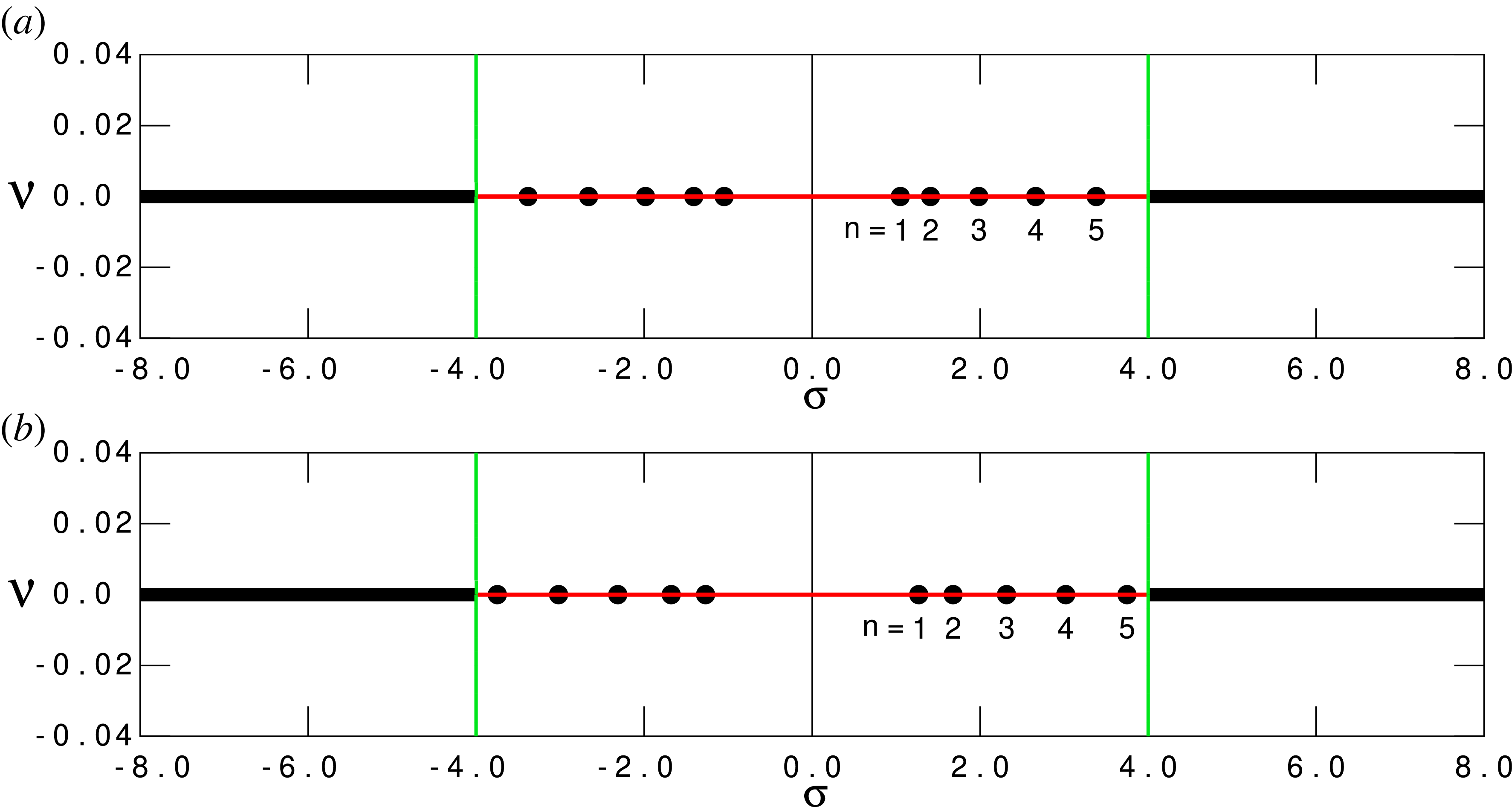
Figure 3 Long description
The image contains two graphs labeled (a) and (b), representing the spectra of conservative normal modes, specifically regular transverse electric (TE) waves in a dielectric medium. Graph (a) shows the even modes, while graph (b) shows the odd modes. Both graphs plot the phase velocity (v) on the y-axis against the wave number in the longitudinal (sigma) direction on the x-axis. The phase velocity changes rapidly from zero to unity in a narrow region just below a specific value. The wave number in the longitudinal direction is denoted as kx. The mode numbering refers to the bound modes, with the propagating (standing) waves for kx constituting continuous spectra. The graphs feature black dots representing data points, a red horizontal line at v equals zero, and green vertical lines at specific sigma values. The data points are labeled with mode numbers from 1 to 5. All values are approximated.
Spectra of quasi-normal modes, i.e. leaky TE modes in the dielectric medium depicted in figure 1: (a) even modes; (b) odd modes. The parameters $\delta$
,
$\delta$
, $\epsilon$
and
$\epsilon$
and $k$
are the same as in figure 3. The mode numbering
$k$
are the same as in figure 3. The mode numbering $n = 1, \ldots, 5$
refers to the unbound (cutoff) discrete modes. Mode numbering of the discrete complex (propagating) modes for
$n = 1, \ldots, 5$
refers to the unbound (cutoff) discrete modes. Mode numbering of the discrete complex (propagating) modes for $|\sigma | \geqslant k$
may be continued with
$|\sigma | \geqslant k$
may be continued with $n = 6, \ldots, \infty$
by exploiting monotonicity along the solution path (red) of the Spectral Web separated by the intersections with the conjugate path (blue). Intersections also appear on the real axis, for
$n = 6, \ldots, \infty$
by exploiting monotonicity along the solution path (red) of the Spectral Web separated by the intersections with the conjugate path (blue). Intersections also appear on the real axis, for $S_{\mathrm{com}} = 0$
, but those ‘solutions’ are spurious since
$S_{\mathrm{com}} = 0$
, but those ‘solutions’ are spurious since $E(1) = 0$
there. The open circles correspond to the standard step function model with
$E(1) = 0$
there. The open circles correspond to the standard step function model with $k = 0$
, where
$k = 0$
, where $\nu = ({{1}/{2}}) \delta \ln [(1 - \delta )/(1 + \delta )]$
.
$\nu = ({{1}/{2}}) \delta \ln [(1 - \delta )/(1 + \delta )]$
.
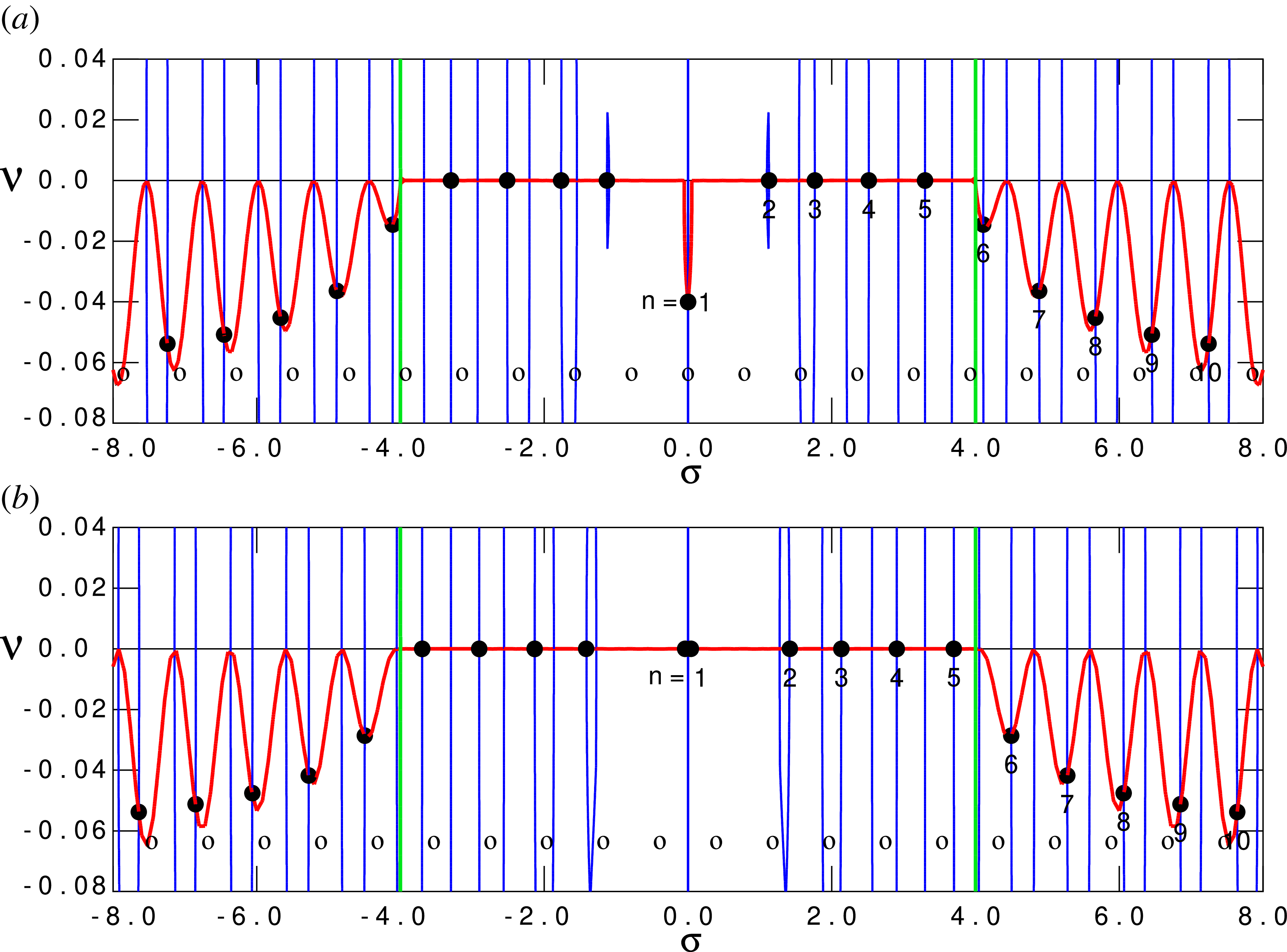
Figure 4 Long description
Two graphs illustrate the spectra of quasi-normal modes, specifically leaky transverse electric modes, in a dielectric medium. The top graph (a) shows even modes, while the bottom graph (b) shows odd modes. Both graphs feature a red line representing the solution path and a blue line representing the conjugate path. The graphs are divided into regions by a hyperbola and lines, with the sign of the external wavenumber indicated in each region. The mode numbering refers to the unbound discrete modes, and the intersections with the conjugate path are marked. The open circles correspond to the standard step function model. The x-axis represents the real part of the wavenumber, and the y-axis represents the imaginary part. The graphs highlight the complex plane divided by the hyperbola and lines, crucial for computing the Spectral Webs.
3.2. Conservative normal modes
The spectra of conservative normal modes are shown in figure 3(a) for the even variety and in figure 3(b) for the odd variety. For all calculations of the present section, the parameters $k = 4.0$
,
$k = 4.0$
, $\delta = 0.25$
and
$\delta = 0.25$
and $\epsilon = 0.02$
were chosen for the purpose of illustration, and also for comparison with earlier calculations by Armitage et al. (Reference Armitage, Doost, Langbein and Mujarov2014). Collecting the expressions for the conservative(
$\epsilon = 0.02$
were chosen for the purpose of illustration, and also for comparison with earlier calculations by Armitage et al. (Reference Armitage, Doost, Langbein and Mujarov2014). Collecting the expressions for the conservative( $\nu = 0$
) bound modes(
$\nu = 0$
) bound modes( $|\sigma | \lt k$
), i.e. in the cutoff region, yields
$|\sigma | \lt k$
), i.e. in the cutoff region, yields
 \begin{equation} \hat {\alpha } = 0,\ \hat {q} = - {\mathrm{i}}\sqrt {k^2 - \sigma ^2} \quad \Rightarrow \ S_{\mathrm{com}} = E(1) [{\mathrm{i}}(\hat {q}_2/\sigma ) E^*(1) - H^*(1)], \end{equation}
where the contribution $S_x(1) \equiv E(1) H^*(1)$
of the internal solution is also imaginary since the basic ODE (2.10) has only real coefficients. This implies that one could choose initial data such that
$S_x(1) \equiv E(1) H^*(1)$
of the internal solution is also imaginary since the basic ODE (2.10) has only real coefficients. This implies that one could choose initial data such that $E(x)$
is real and
$E(x)$
is real and $H(x)$
is imaginary. Choosing complex initial data would not change this conclusion. Hence,
$H(x)$
is imaginary. Choosing complex initial data would not change this conclusion. Hence, $S_{\mathrm{com},1} = 0$
: the solution path is along the real axis, whereas the iterative procedure should produce
$S_{\mathrm{com},1} = 0$
: the solution path is along the real axis, whereas the iterative procedure should produce $S_{\mathrm{com},2} \rightarrow 0$
. For this procedure, there is actually no need to construct the Spectral Web paths in the complex
$S_{\mathrm{com},2} \rightarrow 0$
. For this procedure, there is actually no need to construct the Spectral Web paths in the complex $\omega$
-plane, since the solutions can be obtained by a standard shooting method. The resulting discrete spectra are shown in figure 3 for the mentioned values of
$\omega$
-plane, since the solutions can be obtained by a standard shooting method. The resulting discrete spectra are shown in figure 3 for the mentioned values of $\delta$
and
$\delta$
and $\epsilon$
. In the positive frequency range
$\epsilon$
. In the positive frequency range $0 \lt \sigma \lt k$
, they consist of five even and five odd bound modes, and an equal number of even and odd modes in the negative frequency range. The green lines in figures 3 and 4 indicate the boundaries between the cutoff and propagating regions given by the hyperbola
$0 \lt \sigma \lt k$
, they consist of five even and five odd bound modes, and an equal number of even and odd modes in the negative frequency range. The green lines in figures 3 and 4 indicate the boundaries between the cutoff and propagating regions given by the hyperbola $\sigma ^2 - \nu ^2 = k^2$
of figure 2 (nearly straight lines because of the small vertical section of the
$\sigma ^2 - \nu ^2 = k^2$
of figure 2 (nearly straight lines because of the small vertical section of the $\omega$
-plane).
$\omega$
-plane).
As is well known, the conservative ( $\nu = 0$
) ‘propagating’, or rather standing waves (
$\nu = 0$
) ‘propagating’, or rather standing waves ( $|\sigma | \geqslant k$
), constitute continuous spectra of all real frequencies in those two ranges (see figure 3). Hence, the Spectral Web machinery is not needed either to construct these spectra. This should imply that for all these frequencies, there is no contradiction in satisfying the full BVP, guaranteed by the expressions (2.26), and restricting
$|\sigma | \geqslant k$
), constitute continuous spectra of all real frequencies in those two ranges (see figure 3). Hence, the Spectral Web machinery is not needed either to construct these spectra. This should imply that for all these frequencies, there is no contradiction in satisfying the full BVP, guaranteed by the expressions (2.26), and restricting $\hat {\alpha }$
and
$\hat {\alpha }$
and $\hat {\beta }$
by the condition (2.20). This may be proved by choosing initial data such that
$\hat {\beta }$
by the condition (2.20). This may be proved by choosing initial data such that $E(1) = E_1$
,
$E(1) = E_1$
, $H(1) = {\mathrm{i}} H_2$
, so that the expressions (2.26) become
$H(1) = {\mathrm{i}} H_2$
, so that the expressions (2.26) become
 \begin{eqnarray} &&\hat {\alpha } = {\frac {1}{2}} {\mathrm{e}}^{-{\mathrm{i}}\hat {q}_1} [E_1 + {\mathrm{i}}(\sigma /\hat {q}_1) H_2] ,\quad \hat {\beta } = {\frac {1}{2}} {\mathrm{e}}^{{\mathrm{i}}\hat {q}_1} [E_1 - {\mathrm{i}}(\sigma /\hat {q}_1) H_2],\ \text{with}\ \hat {q}_1 = \sqrt {\sigma ^2 - k^2}, \nonumber \\[4pt] &&\Rightarrow \ \hat {\alpha } = \hat {\beta }{\mathrm{e}}^{-2{\mathrm{i}}\varphi }, \ |\hat {\alpha }| = |\hat {\beta }| = {\frac {1}{2}} \sqrt {E_1^2 + (\sigma H_2/\hat {q}_1)^2} ,\ \varphi = \arctan [\sigma H_2/(\hat {q}_1 E_1)], \end{eqnarray}
QED. Again, this derivation will not change by choosing complex initial data instead. In conclusion, all frequencies satisfying $|\sigma | \geqslant k$
are admitted. The ‘improper eigenfunctions’ associated with these modes are non-square-integrable because of the infinite domain (as in quantum mechanics of free particles). Notice that according to (2.20), no energy is lost at the ends, for
$|\sigma | \geqslant k$
are admitted. The ‘improper eigenfunctions’ associated with these modes are non-square-integrable because of the infinite domain (as in quantum mechanics of free particles). Notice that according to (2.20), no energy is lost at the ends, for $x \rightarrow \infty$
, even though the system is open there.
$x \rightarrow \infty$
, even though the system is open there.
3.3. Quasi-normal, leaky modes
The spectra of leaky modes are shown in figure 4(a) for the even and in figure 4(b) for the odd variety. The parameters are the same as for the conservative modes in § 3.2. According to the expressions (2.21), cutoff leaky modes ( $\sigma ^2 - \nu ^2 \leqslant k^2$
) are restricted to lie either on the real
$\sigma ^2 - \nu ^2 \leqslant k^2$
) are restricted to lie either on the real $\sigma$
-axis or on the negative part of the
$\sigma$
-axis or on the negative part of the $\nu$
-axis:
$\nu$
-axis:
 \begin{align} \hat {\beta } & = 0,\quad \hat {q} = - {\mathrm{i}}\sqrt {k^2 - \omega ^2} \quad \Rightarrow \quad S_{\mathrm{com}} = E(1)\big [f E^*(1) - H^*(1)\big ],\nonumber\\[5pt] &\quad f \equiv \left \{\begin{array}{@{}r@{}l} -{\mathrm{i}}\hat{q}_2/\sigma\ {(\nu = 0),}\\[3pt] \hat {q}_2/\nu\ {(\sigma = 0).} \end{array} \right . \end{align}
Hence, they may be calculated by shooting, as for the conservative bound modes, since the basic ODE (2.10) depends only on the squared frequency $\omega ^2$
(
$\omega ^2$
( $= \sigma ^2$
or
$= \sigma ^2$
or $-\nu ^2$
), which is real. (In figure 4, the Spectral Web contours in the cutoff region are shown anyway to exhibit their peculiar continuation in the propagating region.) Most of the cutoff leaky modes lie on the real
$-\nu ^2$
), which is real. (In figure 4, the Spectral Web contours in the cutoff region are shown anyway to exhibit their peculiar continuation in the propagating region.) Most of the cutoff leaky modes lie on the real $\sigma$
-axis where
$\sigma$
-axis where $S_{\mathrm{com}}$
is imaginary, but some lie on the imaginary
$S_{\mathrm{com}}$
is imaginary, but some lie on the imaginary $\nu$
-axis where
$\nu$
-axis where $S_{\mathrm{com}}$
is real. In this case, there is only one of the latter modes, viz. the degenerate
$S_{\mathrm{com}}$
is real. In this case, there is only one of the latter modes, viz. the degenerate $n = 0$
even mode for
$n = 0$
even mode for $\nu \approx -0.04$
. The
$\nu \approx -0.04$
. The $n = 0$
odd modes lie too close to the origin to see that they are actually non-degenerate:
$n = 0$
odd modes lie too close to the origin to see that they are actually non-degenerate: $\sigma \approx \pm 0.04$
. (Note that the scale along the
$\sigma \approx \pm 0.04$
. (Note that the scale along the $\sigma$
-axis is much larger than along the
$\sigma$
-axis is much larger than along the $\nu$
-axis.) The near vertical blue curves of the conjugate paths actually form closed loops faraway in the
$\nu$
-axis.) The near vertical blue curves of the conjugate paths actually form closed loops faraway in the $\omega$
-plane such that each loop contains just one eigenvalue and one false solution on the real axis. This guarantees monotonicity with arc length of the pertinent component of
$\omega$
-plane such that each loop contains just one eigenvalue and one false solution on the real axis. This guarantees monotonicity with arc length of the pertinent component of $S_{\mathrm{com}}$
in between those points, as generally proved for the analogous quantity
$S_{\mathrm{com}}$
in between those points, as generally proved for the analogous quantity $W_{\mathrm{com}}$
for MHD waves (Goedbloed Reference Goedbloed2018).
$W_{\mathrm{com}}$
for MHD waves (Goedbloed Reference Goedbloed2018).
Finally, propagating leaky modes ( $\sigma ^2 - \nu ^2 \gt k^2$
) have complex values of
$\sigma ^2 - \nu ^2 \gt k^2$
) have complex values of $\omega$
, and hence of
$\omega$
, and hence of $\hat {q}$
, so that the full Spectral Web machinery is needed to calculate their eigenvalues and eigenfunctions. From (2.22), we get the following expression for the complementary Poynting flux exploited in this calculation:
$\hat {q}$
, so that the full Spectral Web machinery is needed to calculate their eigenvalues and eigenfunctions. From (2.22), we get the following expression for the complementary Poynting flux exploited in this calculation:
 \begin{equation} \hat {\beta } = 0,\quad \hat {q} = \pm \sqrt {{\omega ^2} - k^2} \quad \Rightarrow \ S_{\mathrm{com}} = E(1)[(\hat {q}^*/\omega ^*) E^*(1) - H^*(1)]. \end{equation}
The plots of the resulting complex eigenvalues are shown in figure 4(a) for the even modes and in figure 4(b) for the odd modes. Whereas, strictly speaking, the usual labelling by node counting of the eigenfunctions fails for complex eigenvalue problems, the numbering of the complex modes ( $n \geqslant 6$
) can be continued here from the real ones (
$n \geqslant 6$
) can be continued here from the real ones ( $n = 1, \ldots, 5$
) by means of the mentioned monotonicity properties along the paths of the Spectral Web. Nevertheless, it appears to be just a continuation of the numbering for the real ones.
$n = 1, \ldots, 5$
) by means of the mentioned monotonicity properties along the paths of the Spectral Web. Nevertheless, it appears to be just a continuation of the numbering for the real ones.
3.4. Different spectral methods
The spectra shown in figures 3 and 4 agree, qualitatively, with the spectra shown in figure 1 of Armitage et al. (Reference Armitage, Doost, Langbein and Mujarov2014). This reference assumes constant phase velocity in the dielectric slab (of course with a jump at the boundary) as a first approximation to more complicated structures. This paper is one in a sequence of papers (Doost et al. Reference Doost, Langbein and Mujarov2012, Reference Doost, Langbein and Mujarov2013, Reference Doost, Langbein and Mujarov2014) on the so-called resonant state expansion of ever more complicated systems, where the central dielectric slab is modified, e.g. with layers of different values of the phase velocity. This includes frequency-dependent ones (Muljarov & Langbein Reference Muljarov and Langbein2016) and even anisotropic magnetic materials (Muljarov & Weiss Reference Muljarov and Weiss2018). Likewise, Upendar et al. (Reference Upendar, Allayarov, Schmidt and Weiss2018) investigate the properties of different optical fibre systems with such a method. The resulting complicated spectrum is computed by means of a perturbation method based on the simple unperturbed constant phase velocity model, exploiting Greens function techniques (to be discussed in § 4.1 on the initial value problem). This computation requires solving a nonlinear eigenvalue problem with a large number of modes of the unperturbed system.
In the Spectral Web method, this part of the mentioned procedure is replaced by the numerical integration of the ODEs in the internal region since it automatically adjusts the integration step to enforce continuity of $E(x)$
and
$E(x)$
and $H(x)$
at the boundaries of the different internal domains where a discontinuous phase velocity profile is prescribed. The solution of the resulting spectral problem is then concentrated in solely computing the complementary Poynting flux and the associated paths in the complex plane at the final outer boundary
$H(x)$
at the boundaries of the different internal domains where a discontinuous phase velocity profile is prescribed. The solution of the resulting spectral problem is then concentrated in solely computing the complementary Poynting flux and the associated paths in the complex plane at the final outer boundary $|x| = 1$
of the inhomogeneous region. In the present case, obtaining the external solutions
$|x| = 1$
of the inhomogeneous region. In the present case, obtaining the external solutions $\hat {E}(x)$
and
$\hat {E}(x)$
and $\hat {H}(x)$
is completely explicit through the inversion of the external dispersion equation (2.14). For non-trivial more-dimensional external structures, numerical integration over the external region satisfying the outflow BC would be necessary. This may be performed, for arbitrarily chosen complex values of
$\hat {H}(x)$
is completely explicit through the inversion of the external dispersion equation (2.14). For non-trivial more-dimensional external structures, numerical integration over the external region satisfying the outflow BC would be necessary. This may be performed, for arbitrarily chosen complex values of $\omega$
, virtually without any approximation since the required accuracy of modern numerical solvers may be prescribed. The eigenvalues themselves are then obtained from the zeros of the complementary Poynting flux in the next step of the procedure.
$\omega$
, virtually without any approximation since the required accuracy of modern numerical solvers may be prescribed. The eigenvalues themselves are then obtained from the zeros of the complementary Poynting flux in the next step of the procedure.
3.5. CNM and QNM eigenfunctions
Characteristic eigenfunctions in the cutoff and standing-wave/propagating regions are respectively shown in figures 5(a) and 5(b) for the conservative modes (labelled by the mode number $n$
in the spectra of figure 3), and in figures 6(a) and 6(b) for the leaky modes (labelled by the mode number
$n$
in the spectra of figure 3), and in figures 6(a) and 6(b) for the leaky modes (labelled by the mode number $n$
in the spectra of figure 4). To save space, only the electric fields are exhibited and the associated magnetic fields have been omitted. Their amplitudes are indicated though. Peculiarly, all amplitude changes of the magnetic field in the very narrow region of inhomogeneity (better visible in the wider regions of their MHD counterparts
$n$
in the spectra of figure 4). To save space, only the electric fields are exhibited and the associated magnetic fields have been omitted. Their amplitudes are indicated though. Peculiarly, all amplitude changes of the magnetic field in the very narrow region of inhomogeneity (better visible in the wider regions of their MHD counterparts $\varPi$
and
$\varPi$
and $\xi$
in figures 9 and 10) are opposite to those of the electric fields.
$\xi$
in figures 9 and 10) are opposite to those of the electric fields.
CNM eigenfunctions corresponding to the spectrum depicted in figure 3(a) for the even modes: (a) a discrete bound mode with $n = 5$
and
$n = 5$
and $\sigma = 3.3813$
on the interval
$\sigma = 3.3813$
on the interval $(0, 8.0)$
; (b) a ‘propagating’ continuum mode with the arbitrary choice
$(0, 8.0)$
; (b) a ‘propagating’ continuum mode with the arbitrary choice $\sigma = 6.0$
of the improper eigenvalue on the same interval. The phase velocity profile
$\sigma = 6.0$
of the improper eigenvalue on the same interval. The phase velocity profile $v(x)$
for this interval is depicted above the eigenfunctions. The parameters
$v(x)$
for this interval is depicted above the eigenfunctions. The parameters $\delta$
,
$\delta$
, $\epsilon$
and
$\epsilon$
and $k$
are the same as in figure 3. The amplitudes of the associated functions
$k$
are the same as in figure 3. The amplitudes of the associated functions $H_{1,2}(x)$
, which are not displayed, decrease across the inhomogeneous boundary layer (in contrast to the functions
$H_{1,2}(x)$
, which are not displayed, decrease across the inhomogeneous boundary layer (in contrast to the functions $E_{1,2}(x)$
which increase). Their amplitudes at
$E_{1,2}(x)$
which increase). Their amplitudes at $|x| = 1$
are given in the top right of the figures.
$|x| = 1$
are given in the top right of the figures.
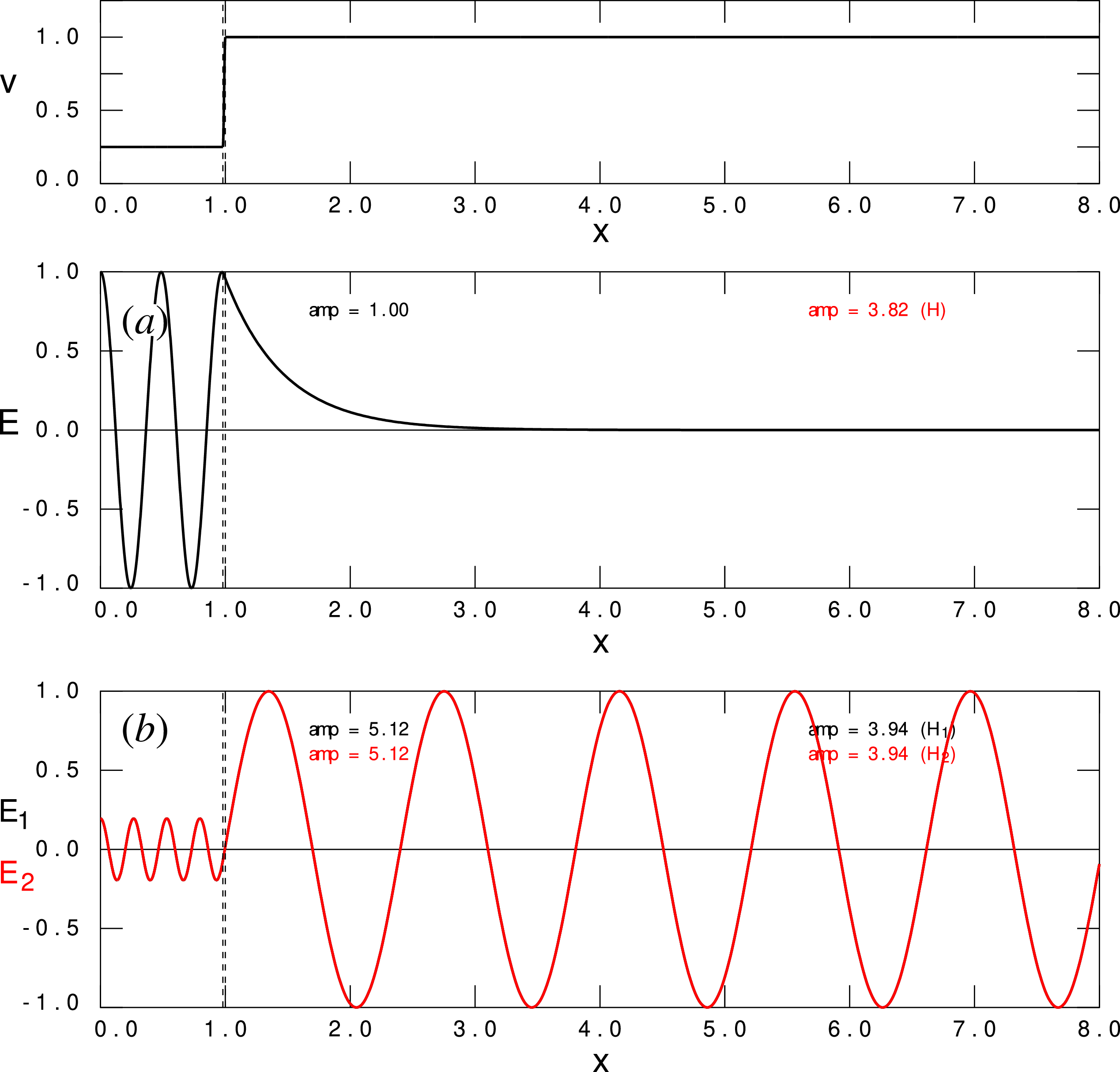
Figure 5 Long description
The image contains three graphs. The top graph shows the phase velocity profile as a function of position X, with a sharp transition at X equals 1. The middle graph displays the eigenfunction E for a discrete bound mode, with an amplitude of 1.00 inside the interval and 3.82 outside. The bottom graph presents two eigenfunctions, E1 and E2, for a propagating continuum mode, with amplitudes of 5.12 and 3.94 respectively, and an improper eigenvalue. The eigenfunctions exhibit oscillatory behavior within the interval and decay outside. The amplitudes of the associated functions at X equals 1 are provided in the top right of the graphs.
The conservative modes are divided in bound modes for $|\sigma | \lt k$
, which are oscillatory for
$|\sigma | \lt k$
, which are oscillatory for $|x| \lt 1$
but evanescent for
$|x| \lt 1$
but evanescent for $|x| \geqslant 1$
(figure 5
a), and standing waves for
$|x| \geqslant 1$
(figure 5
a), and standing waves for $|\sigma | \geqslant k$
, which are oscillatory in both regions but with different wavelengths (figure 5
b). The bound modes are discrete, but the standing waves form continuous spectra since their domain is infinite in
$|\sigma | \geqslant k$
, which are oscillatory in both regions but with different wavelengths (figure 5
b). The bound modes are discrete, but the standing waves form continuous spectra since their domain is infinite in $x$
. This infinite domain is representative of an open boundary but, since the amplitudes of the standing waves are constant, no energy is lost at infinity!
$x$
. This infinite domain is representative of an open boundary but, since the amplitudes of the standing waves are constant, no energy is lost at infinity!
The leaky modes are also distinguished in two kinds of modes: so-called cutoff modes for $|\sigma | \lt k$
, which are partly oscillatory in the region
$|\sigma | \lt k$
, which are partly oscillatory in the region $|x| \lt 1$
and exponentially growing for
$|x| \lt 1$
and exponentially growing for $|x| \geqslant 1$
(figure 6
a), and propagating waves for
$|x| \geqslant 1$
(figure 6
a), and propagating waves for $|\sigma | \geqslant k$
, which oscillate in both regions, again with different wavelengths, but their amplitude is exponentially growing in the external region (figure 6
b). The explosive growth of the leaky modes for
$|\sigma | \geqslant k$
, which oscillate in both regions, again with different wavelengths, but their amplitude is exponentially growing in the external region (figure 6
b). The explosive growth of the leaky modes for $x \rightarrow \infty$
results in exponentially infinite energy loss there! Associated with this spatial growth is the temporal damping
$x \rightarrow \infty$
results in exponentially infinite energy loss there! Associated with this spatial growth is the temporal damping $\nu \lt 0$
of the modes. Clearly, in contrast to unstable systems where the perturbations are assumed to grow from tiny fluctuations of the background, leaky modes can not appear in this way. They require finite initial perturbations, as discussed in the next section. How the infinite energy flux for
$\nu \lt 0$
of the modes. Clearly, in contrast to unstable systems where the perturbations are assumed to grow from tiny fluctuations of the background, leaky modes can not appear in this way. They require finite initial perturbations, as discussed in the next section. How the infinite energy flux for $|x| \rightarrow \infty$
is sidestepped for TE modes is the subject of § 4.2. Whether this ‘magic’ also works for MHD waves in coronal flux tubes will be investigated in § 7.
$|x| \rightarrow \infty$
is sidestepped for TE modes is the subject of § 4.2. Whether this ‘magic’ also works for MHD waves in coronal flux tubes will be investigated in § 7.
Since the exponentially explosive part of the cutoff leaky modes solution is restricted to the external part ( $|x| \gt 1$
), the oscillations of the internal part may be exploited to label the solutions with their number of nodes (never mind that they also may have a large, but not infinite, amplitude for
$|x| \gt 1$
), the oscillations of the internal part may be exploited to label the solutions with their number of nodes (never mind that they also may have a large, but not infinite, amplitude for $|x| \leqslant 1$
). Significantly, the bound conservative modes are solutions of the same Sturm–Liouvile type ODE (2.10)! This permits to arrange the sequences of discrete eigenvalues of the leaky modes (subscript
$|x| \leqslant 1$
). Significantly, the bound conservative modes are solutions of the same Sturm–Liouvile type ODE (2.10)! This permits to arrange the sequences of discrete eigenvalues of the leaky modes (subscript $\mathrm{L}$
) in an interweaving pattern with those of the conservative bound modes (subscript
$\mathrm{L}$
) in an interweaving pattern with those of the conservative bound modes (subscript $\mathrm{C}$
), distinguishing between even and odd (subscripts
$\mathrm{C}$
), distinguishing between even and odd (subscripts $\mathrm{e}$
and
$\mathrm{e}$
and $\mathrm{o}$
), according to the following scheme:
$\mathrm{o}$
), according to the following scheme:
 \begin{equation} |\nu _{{\mathrm{L}}{1{\mathrm{e}}}}| \lt |\sigma _{{\mathrm{C}}{1{\mathrm{e}}}}| \lt |\sigma _{{\mathrm{L}}{1{\mathrm{o}}}}| \lt |\sigma _{{\mathrm{C}}{1{\mathrm{o}}}}| \lt |\sigma _{{\mathrm{L}}{2{\mathrm{e}}}}| \lt |\sigma _{{\mathrm{C}}{2{\mathrm{e}}}}| \lt |\sigma _{{\mathrm{L}}{2{\mathrm{o}}}}| \lt |\sigma _{{\mathrm{C}}{2{\mathrm{o}}}}| \ldots (\lt k) . \end{equation}
The explicit eigenvalues of these sequences are given in table 1(a). They are completed with the complex eigenvalues of the propagating leaky modes in table 1(b). Since the conjugate paths are nearly vertical close to the crossings with the solution path, extremely fast and accurate convergence to those eigenvalues is obtained by just iterating along the relevant conjugate path. The numbers obtained are truncated to five decimal places (more than enough for the present purpose). Of course, the real counterparts of the standing conservative modes are missing since they occupy all real numbers $\geqslant k$
.
$\geqslant k$
.
Connection between the different modes of the spectra depicted in figures 3 and 4. Alternating real frequencies of the even leaky (L ne ), the even conservative (C ne ), the odd leaky (L no ) and the odd conservative (C no ) modes in the cutoff region. The first two leaky modes (n = ‘1’) immediately start to diverge away from |x| = 0 so that they strictly fall outside the alternating n > 1 sequences, which are based on monotonicity along the solution path. Complex frequencies of the even (L ne ) and odd (L no ) propagating leaky modes. Beyond cutoff, the real frequencies of the even/odd conservative modes form continua of standing waves.
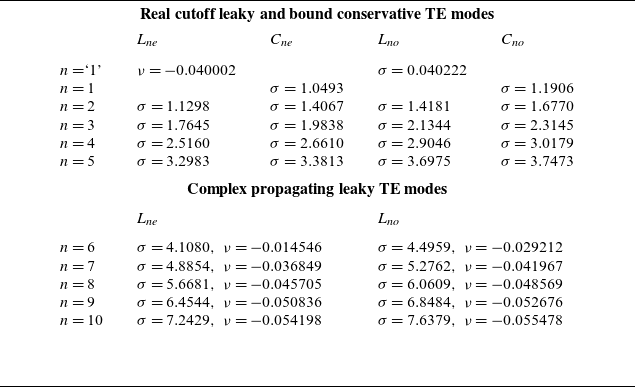
Table 1 Long description
A table comparing real and complex frequencies of different modes in cutoff and propagating regions. The table is divided into two sections: Real cutoff leaky and bound conservative TE modes, and Complex propagating leaky TE modes. The first section lists the real frequencies for even leaky (Lne), even conservative (Cne), odd leaky (Lno), and odd conservative (Cno) modes for values of n ranging from 1 to 5. The second section lists the complex frequencies for even (Lne) and odd (Lno) propagating leaky modes for values of n ranging from 6 to 10. Each section includes columns for the mode type, the value of n, the real part of the frequency (v), and the imaginary part of the frequency (sigma). The table provides detailed numerical values for each mode and frequency combination.
QNM eigenfunctions corresponding to the spectrum depicted in figure 4(a) for the even modes. (a) A real, unbound, discrete mode with $n = 4$
and
$n = 4$
and $\sigma = 3.2983$
on the interval
$\sigma = 3.2983$
on the interval $(0, 8.0)$
. Since the exponential growth is huge, the eigenfunction has been magnified by the factor
$(0, 8.0)$
. Since the exponential growth is huge, the eigenfunction has been magnified by the factor $10^6$
(dashed curves) to show the oscillations on the internal part of the interval. (b) A complex, leaky, discrete mode with
$10^6$
(dashed curves) to show the oscillations on the internal part of the interval. (b) A complex, leaky, discrete mode with $n = 9$
and
$n = 9$
and $\sigma = 6.4545$
,
$\sigma = 6.4545$
, $\nu = - 0.050836$
on the same interval. The parameters
$\nu = - 0.050836$
on the same interval. The parameters $\delta$
,
$\delta$
, $\epsilon$
and
$\epsilon$
and $k$
are the same as in figure 3.
$k$
are the same as in figure 3.
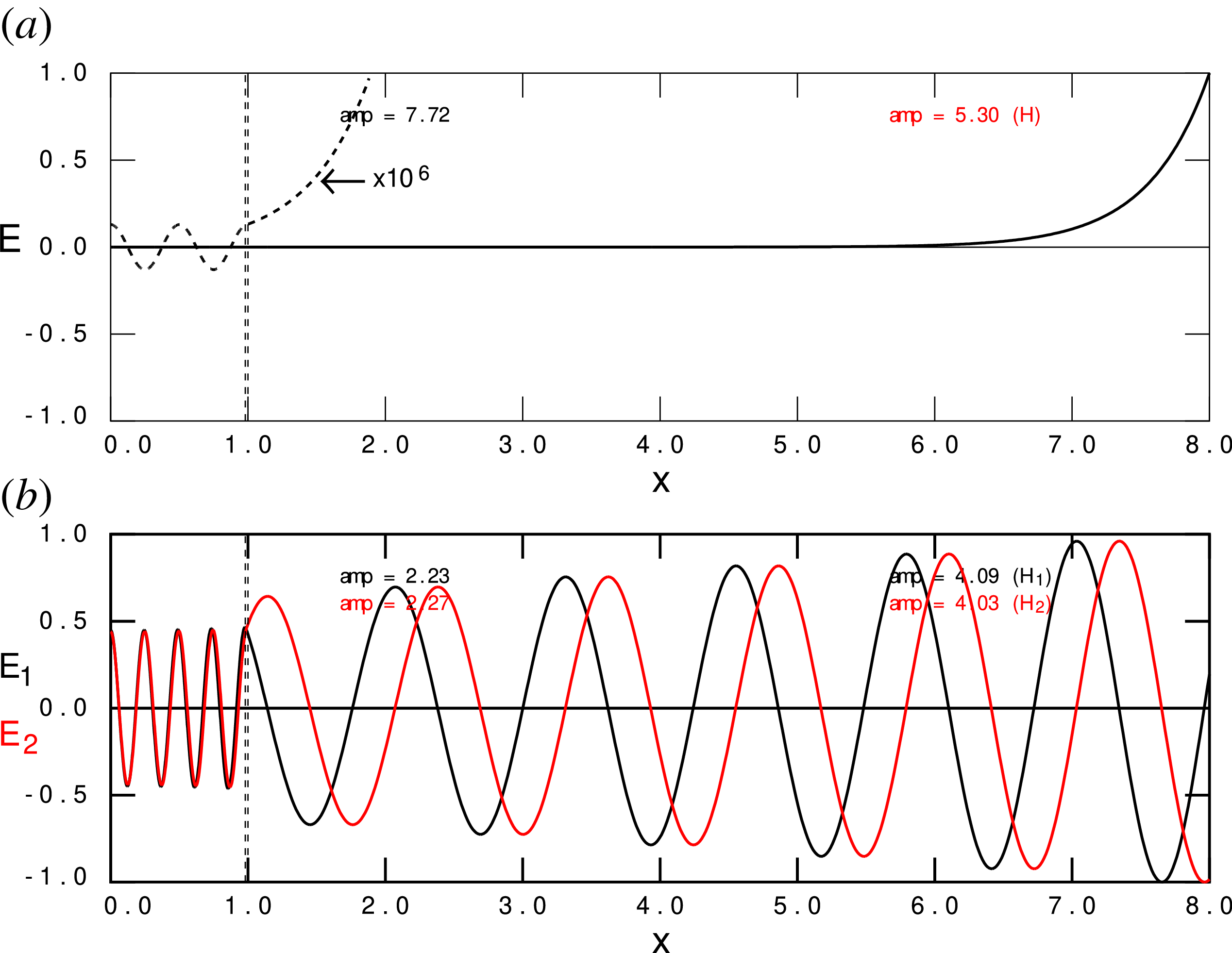
Figure 6 Long description
The image contains two graphs labeled (a) and (b) showing spectra with different modes and parameters. Graph (a) depicts a real, unbound, discrete mode with specific parameters on the interval. The eigenfunction is magnified by a factor to show oscillations on the internal part of the interval. Graph (b) shows a complex, leaky, discrete mode with different parameters on the same interval. Both graphs illustrate the spectra corresponding to the even modes, with the parameters consistent with those in a previous figure. The spectra agree qualitatively with those in a referenced study, assuming constant phase velocity in the dielectric slab as a first approximation. The computation involves solving a nonlinear eigenvalue problem with a large number of modes of the unperturbed system.
The frequency scheme of table 1 consists of numbers that depend on the specific inhomogeneity of the internal region only: perfect for classical (non-quantum mechanical) spectroscopy to determine the structure of dielectric materials with external excitation, that is, if only the infinities can be avoided, which is the subject of the next section.
4. Excitation of conservative and leaky electromagnetic waves
4.1. Initial value problem
So far, we have presented conservative and leaky modes on an equal footing but, obviously, one physical system cannot be described by two different eigenvalue spectra. The pertinent question to be answered is: when is the conservative picture appropriate and when does the leaky mode picture apply? Broadly speaking, the regular conservative picture provides the final, stationary state response of the system to excitation, whereas the leaky mode picture provides a description of the response of the system in the initial phase when, so to speak, the outward waves do not yet ‘know’ that they are on the way to infinity and assumed to grow without bound. The latter description has been accepted for electromagnetic waves for a long time, and for the obvious reason that it is observed, but only rather recently has it been provided with a theoretical description on par with the standard description of conservative modes in terms of self-adjoint operators in Hilbert space; see the tutorial by Sauvan et al. (Reference Sauvan, Wu, Zarouf, Muljarov and Lalanne2022). This distinct description of leaky modes, called ‘regularisation’, is the subject of the following sub-section. Before discussing that, we first present what is common to the two descriptions.
To describe the response to excitation of TE modes, the usual formulation of the solution of the initial value problem in terms of Green’s functions is most effective. Exploiting the formulation of our textbook (Goedbloed et al. Reference Goedbloed, Keppens and Poedts2019), we transform the prospective time-dependent solution $E(x;t)$
to the frequency-dependent variable
$E(x;t)$
to the frequency-dependent variable $\widetilde {E}(x;\omega )$
by means of the f orward Laplace transformation,
$\widetilde {E}(x;\omega )$
by means of the f orward Laplace transformation,
 \begin{equation} \widetilde {E}(x;\omega ) \equiv \int _0^\infty {\!\!}E(x;t) {\mathrm{e}}^{{\mathrm{i}}\omega t} {\rm d}{\,}t . \end{equation}
The original time-evolution equation (2.4), simplified for the present TE modes to
 \begin{equation} \frac {1}{v^2}\frac {\partial ^2 E}{\partial t^2} - \frac {\partial ^2 E}{\partial x^2} + k^2 E = 0 , \end{equation}
is also subjected to that transformation:
 \begin{equation} \frac {\mathrm{d}^2 \widetilde {E}}{{\rm d}x^2} + (\omega ^2/v^2 - k^2) \widetilde {E} = ({\mathrm{i}}\omega E_{\mathrm{i}}(x) - \dot {E}_{\mathrm{i}}(x))/v^2 \equiv X(x;\omega ) . \end{equation}
Here, the excitation $X = X(x;\omega )$
is assumed to be known from prescribed initial data
$X = X(x;\omega )$
is assumed to be known from prescribed initial data $E_{\mathrm{i}}(x) \equiv E(x; t = 0)$
and
$E_{\mathrm{i}}(x) \equiv E(x; t = 0)$
and $\dot {E}_{\mathrm{i}}(x) \equiv {\partial E/\partial t}(x; t = 0)$
. Those are obtained from the Laplace transform of the first term of (4.2) by integrating by parts and neglecting the terms multiplying
$\dot {E}_{\mathrm{i}}(x) \equiv {\partial E/\partial t}(x; t = 0)$
. Those are obtained from the Laplace transform of the first term of (4.2) by integrating by parts and neglecting the terms multiplying $\exp ({{\mathrm{i}}\omega t})$
for
$\exp ({{\mathrm{i}}\omega t})$
for $t \rightarrow \infty$
since they vanish in the upper part of the complex
$t \rightarrow \infty$
since they vanish in the upper part of the complex $\omega$
-
plane. This restriction will be removed later by means of analytic continuation.
$\omega$
-
plane. This restriction will be removed later by means of analytic continuation.
The inhomogeneous ODE (4.3) is solved by the integral
 \begin{equation} \widetilde {E}(x;\omega ) = \int _0^\infty G(x,x^{\prime};\omega ) X(x^{\prime};\omega ) {\rm d}x^{\prime} , \end{equation}
where the Green’s function $G(x,x^{\prime};\omega )$
satisfies another inhomogeneous ODE,
$G(x,x^{\prime};\omega )$
satisfies another inhomogeneous ODE,
 \begin{equation} \left[ \frac {{\rm d}^2 }{{\rm d}x^2} + \omega ^2/v^2 - k^2 \right] G(x,x^{\prime};\omega ) = \delta (x - x^{\prime}) , \end{equation}
subject to the left BC at $x = 0$
, the right BC for
$x = 0$
, the right BC for $x \rightarrow \infty$
, continuity,
$x \rightarrow \infty$
, continuity, $\lbrack \!\lbrack G \rbrack \!\rbrack = 0$
, and unit jump of the derivative,
$\lbrack \!\lbrack G \rbrack \!\rbrack = 0$
, and unit jump of the derivative, $\lbrack \!\lbrack {\rm d}G/{\rm d}x \rbrack \!\rbrack = 1$
, at the joining point
$\lbrack \!\lbrack {\rm d}G/{\rm d}x \rbrack \!\rbrack = 1$
, at the joining point $x = x^{\prime}$
. The explicit solution of (4.5) is then given by the quotient
$x = x^{\prime}$
. The explicit solution of (4.5) is then given by the quotient
 \begin{equation} G(x,x^{\prime};\omega ) = \frac {\varGamma (x,x^{\prime};\omega )}{\Delta (\omega )} , \end{equation}
where the numerator and denominator are composed of the left and right solutions, $U_1(x;\omega )$
and
$U_1(x;\omega )$
and $U_2(x;\omega )$
, of the original homogeneous ODE (2.10),
$U_2(x;\omega )$
, of the original homogeneous ODE (2.10),
 \begin{eqnarray} \varGamma (x,x^{\prime};\omega ) &\,=\,& U_1(x;\omega ) U_2(x^{\prime};\omega ) H(x^{\prime} - x) + U_1(x^{\prime};\omega ) U_2(x;\omega ) H(x - x^{\prime}), \nonumber \\[5pt] \Delta (\omega ) &\,=\,& U_1(x;\omega ) U^{\prime}_2(x;\omega ) - U^{\prime}_1(x;\omega ) U_2(x;\omega ) , \end{eqnarray}
and $H$
here indicates the Heaviside function. The Wronskian
$H$
here indicates the Heaviside function. The Wronskian $\varDelta$
is independent of
$\varDelta$
is independent of $x$
as a direct consequence of the differential equation. In this manner, the numerical solution (2.12) and the analytical solution (2.13) of § 2.3 return:
$x$
as a direct consequence of the differential equation. In this manner, the numerical solution (2.12) and the analytical solution (2.13) of § 2.3 return: $U_1(x;\omega ) \equiv E(x;\omega )$
for
$U_1(x;\omega ) \equiv E(x;\omega )$
for $|x| \leqslant 1$
and
$|x| \leqslant 1$
and $U_2(x;\omega ) \equiv \hat {E}(x;\omega )$
for
$U_2(x;\omega ) \equiv \hat {E}(x;\omega )$
for $|x| \gt 1$
. However, the important difference is that the left solution
$|x| \gt 1$
. However, the important difference is that the left solution $U_1$
, satisfying the BC (2.23) at
$U_1$
, satisfying the BC (2.23) at $x = 0$
, is continuously extended into the right part, and the right solution, satisfying either one of the BCs (2.25) at
$x = 0$
, is continuously extended into the right part, and the right solution, satisfying either one of the BCs (2.25) at $x \rightarrow \infty$
, is continuously extended into the left part. These extensions demand that the corresponding electric and magnetic fields do not jump at
$x \rightarrow \infty$
, is continuously extended into the left part. These extensions demand that the corresponding electric and magnetic fields do not jump at $|x| = 1$
, i.e.
$|x| = 1$
, i.e. $\lbrack \!\lbrack U_i \rbrack \!\rbrack = 0$
and
$\lbrack \!\lbrack U_i \rbrack \!\rbrack = 0$
and $\lbrack \!\lbrack U^{\prime}_i \rbrack \!\rbrack = 0$
, where
$\lbrack \!\lbrack U^{\prime}_i \rbrack \!\rbrack = 0$
, where $i = 1, 2$
. In general, this implies that the two solutions do not satisfy the required BCs at the other end, so that
$i = 1, 2$
. In general, this implies that the two solutions do not satisfy the required BCs at the other end, so that $U_1$
and
$U_1$
and $U_2$
are not eigenfunctions.
$U_2$
are not eigenfunctions.
At this point, it is expedient to convert the expression (4.7) for $\varDelta$
, which may also be called the dispersion function, into the physical variables
$\varDelta$
, which may also be called the dispersion function, into the physical variables $E$
and
$E$
and $H$
at the position
$H$
at the position $x = 1$
(i.e. at the position where the extensions of
$x = 1$
(i.e. at the position where the extensions of $U_1$
and
$U_1$
and $U_2$
are not relevant):
$U_2$
are not relevant):
 \begin{equation} \varDelta = ({\mathrm{i}}/\omega ) [E(1;\omega ) \hat {H}(1;\omega ) - H(1;\omega ) \hat {E}(1;\omega )] = ({\mathrm{i}}/\omega )E(1;\omega ) \lbrack \!\lbrack H(1;\omega ) \rbrack \!\rbrack , \end{equation}
where the arbitrary amplitudes of the two functions $U_1$
and
$U_1$
and $U_2$
have been chosen to correspond to the same electric field at
$U_2$
have been chosen to correspond to the same electric field at $x = 1$
. For eigenvalues
$x = 1$
. For eigenvalues $\omega = \omega _n$
, the two functions
$\omega = \omega _n$
, the two functions $U_1$
and
$U_1$
and $U_2$
become identical (and eigenfunctions), so that
$U_2$
become identical (and eigenfunctions), so that
 \begin{equation} U_1(x;\omega _n) = U_2(x;\omega _n) \equiv E(x;\omega _n) \quad \text{for all }x \quad \Rightarrow \quad \Delta (\omega _n) = 0 , \end{equation}
where, from now on, the physical variable $E(x;\omega _n)$
indicates both the internal numerical part and (dropping the hat) also the external analytical part of the solution.
$E(x;\omega _n)$
indicates both the internal numerical part and (dropping the hat) also the external analytical part of the solution.
As a side remark, note that there is an obvious relation with the complementary Poynting flux (2.29) of § 2. Since $\lbrack \!\lbrack H(1;\omega ) \rbrack \!\rbrack = \exp (2{\mathrm{i}}\zeta ) \lbrack \!\lbrack H^*(1;\omega ) \rbrack \!\rbrack$
, with the phase angle
$\lbrack \!\lbrack H(1;\omega ) \rbrack \!\rbrack = \exp (2{\mathrm{i}}\zeta ) \lbrack \!\lbrack H^*(1;\omega ) \rbrack \!\rbrack$
, with the phase angle $\zeta = \zeta (\omega )$
, the two are directly related:
$\zeta = \zeta (\omega )$
, the two are directly related:
 \begin{equation} \Delta (\omega ) = f(\omega ) S_{\mathrm{com}}(\omega ),\quad f(\omega ) \equiv ({\mathrm{i}}/\omega ) {\mathrm{e}}^{2{\mathrm{i}} \zeta (\omega )} . \end{equation}
Hence, one may construct Spectral Webs just as well from $\Delta (\omega )$
as from
$\Delta (\omega )$
as from $S_{\mathrm{com}}(\omega )$
. They will give different solution and conjugate paths in the complex
$S_{\mathrm{com}}(\omega )$
. They will give different solution and conjugate paths in the complex $\omega$
-plane, but their crossings will occur at the same eigenvalue positions.
$\omega$
-plane, but their crossings will occur at the same eigenvalue positions.
At the eigenvalue frequencies $\omega = \omega _n$
, the numerator of the Green’s function quotient simplifies to
$\omega = \omega _n$
, the numerator of the Green’s function quotient simplifies to
 \begin{equation} \varGamma (x,x^{\prime};\omega _n) = E(x;\omega _n) E(x^{\prime};\omega _n) , \end{equation}
whereas the denominator may be expanded:
 \begin{align} \Delta (\omega ) \approx (\omega - \omega _n) \left[\frac {\partial \Delta }{\partial \omega }\right]_{\omega _n} \!\!\!\approx (\omega - \omega _n) A_n, \qquad A_n \equiv \left[ ({{\mathrm{i}}}/{\omega }) E(1;\omega ) \frac {\partial \lbrack \!\lbrack {H(1;\omega )}\rbrack \!\rbrack }{\partial \omega } \right]_{\omega _n} .\nonumber\\[-14pt]\nonumber\\ \end{align}
The constants $A_n$
may be computed and then eliminated by normalising the solutions
$A_n$
may be computed and then eliminated by normalising the solutions $E_n = E(x;\omega _n)$
such that these constants become equal to
$E_n = E(x;\omega _n)$
such that these constants become equal to $1$
, so that they disappear from the Green’s function in the neighbourhood of the eigenvalue
$1$
, so that they disappear from the Green’s function in the neighbourhood of the eigenvalue $\omega _n$
:
$\omega _n$
:
 \begin{equation} G(x,x^{\prime};\omega ) \approx \frac {E(x;\omega _n) E(x^{\prime};\omega _n)}{\omega - \omega _n} . \end{equation}
Green’s function is now sufficiently explicit in terms of the eigenfunctions to construct the final solution of the initial value problem.
That final solution involves the inverse Laplace transformation,
 \begin{equation} E(x;t) \equiv \frac {1}{2\pi }\int _{C_0} \!\!{\rm d}\omega\, {\mathrm{e}}^{-{\mathrm{i}}\omega t} \!\int _0^\infty G(x,x^{\prime};\omega ) {\,}X(x^{\prime};\omega ) {\,}{\rm d}x^{\prime} , \end{equation}
where $C_0$
indicates a line from
$C_0$
indicates a line from $\omega = -\infty + {\mathrm{i}}\nu _0$
to
$\omega = -\infty + {\mathrm{i}}\nu _0$
to $\omega = \infty + {\mathrm{i}}\nu _0$
, with
$\omega = \infty + {\mathrm{i}}\nu _0$
, with $\nu _0 \gt 0$
, in the upper half of the
$\nu _0 \gt 0$
, in the upper half of the $\omega$
-plane. To exploit analytic continuation, this line is connected with a downward/upward contour into the bottom half of the
$\omega$
-plane. To exploit analytic continuation, this line is connected with a downward/upward contour into the bottom half of the $\omega$
-plane, e.g. a semi-circle of radius
$\omega$
-plane, e.g. a semi-circle of radius $R \rightarrow \infty$
. The integral over that additional piece vanishes, so that the line integral (4.14) over
$R \rightarrow \infty$
. The integral over that additional piece vanishes, so that the line integral (4.14) over $C_0$
is transformed into a contour integral over the closed curve
$C_0$
is transformed into a contour integral over the closed curve $C$
with the same value. That contour is deformed into the lower half of the
$C$
with the same value. That contour is deformed into the lower half of the $\omega$
-plane encircling the eigenvalues
$\omega$
-plane encircling the eigenvalues $\omega = \omega _n$
, so that the Cauchy residue theorem, or rather the Mittag–Leffler theorem, yields the value of the contour integral and, hence, the solution of the initial value problem for systems with discrete eigenvalues:
$\omega = \omega _n$
, so that the Cauchy residue theorem, or rather the Mittag–Leffler theorem, yields the value of the contour integral and, hence, the solution of the initial value problem for systems with discrete eigenvalues:
 \begin{eqnarray} E(x;t) &\,=\,& \sum _{\omega _n} {\mathrm{e}}^{-{\mathrm{i}}{\omega _n}t} \!\int _0^\infty {\mathrm{Res}} \big \{G(x,x^{\prime};\omega )\big \}_{\omega _n} X(x^{\prime};\omega _n) {\,}{\rm d}x^{\prime} \nonumber \\ &\,=\,& \sum _{\omega _n} {E(x;\omega _n)}{\mathrm{e}}^{-{\mathrm{i}}{\omega _n}t} \!\int _0^\infty E(x^{\prime};\omega _n) {\,}X(x^{\prime};\omega _n) {\,}{\rm d}x^{\prime} . \end{eqnarray}
In the last equality, the expressions (2.11) and (2.12) for $\varGamma$
and
$\varGamma$
and $\varDelta$
have been inserted. This yields the standard solution of the conservative spectral problem when the continuum is approximated by a collection of closely packed discrete eigenvalues. The exact expression for the continuum contribution by an integral over the spectral cuts
$\varDelta$
have been inserted. This yields the standard solution of the conservative spectral problem when the continuum is approximated by a collection of closely packed discrete eigenvalues. The exact expression for the continuum contribution by an integral over the spectral cuts $\sigma \geqslant k$
and
$\sigma \geqslant k$
and $\sigma \leqslant -k$
is omitted since the standard conservative picture is not our main concern here. Rather, we will demonstrate how the usual orthonormality conditions entering in the CNM eigenfunction expansions are modified for the QNMs.
$\sigma \leqslant -k$
is omitted since the standard conservative picture is not our main concern here. Rather, we will demonstrate how the usual orthonormality conditions entering in the CNM eigenfunction expansions are modified for the QNMs.
4.2. Orthogonality and normalisation
The final distinction between conservative and leaky modes comes from the different orthogonality relations of the modes and the different normalisations connected with them. In particular, the solution (4.15) of the initial value problem does not make sense at all for the leaky modes because the exponential explosion at infinity prevents expanding the constituent functions $E(x;\omega _n)$
of the Green’s function in regular square integrable functions. To produce meaningful results, these functions need to be regularised. This is the subject of sub-section § 4.2.2.
$E(x;\omega _n)$
of the Green’s function in regular square integrable functions. To produce meaningful results, these functions need to be regularised. This is the subject of sub-section § 4.2.2.
General orthogonality and normalisation relations, both for conservative and for leaky modes, are obtained from (2.3) by considering two modes satisfying the respective equations for the frequencies $\omega _n$
and
$\omega _n$
and $\omega _m$
:
$\omega _m$
:
 \begin{align} - {\mathrm{i}}(\omega _n/v^2) \mathbf{E}_n = \boldsymbol{\nabla }\times \mathbf{H}_n , \qquad - {\mathrm{i}}\omega _n \mathbf{H}_n = - \boldsymbol{\nabla }\times \mathbf{E}_n , \end{align}
 \begin{align} - {\mathrm{i}}(\omega _m/v^2) \mathbf{E}_m = \boldsymbol{\nabla }\times \mathbf{H}_m , \qquad - {\mathrm{i}}\omega _m \mathbf{H} _m = - \boldsymbol{\nabla }\times \mathbf{E}_m . \end{align}
Quadratic forms are constructed from these equations by means of inner products, integrated over all space and reduced with the divergence theorem, schematically:
 \begin{equation} \int \{[{(4.16a)} \boldsymbol{\cdot }\mathbf{E}_m - {(4.17a)} \boldsymbol{\cdot }\mathbf{E}_n] \pm [{(4.16b)} \boldsymbol{\cdot }\mathbf{H}_m - {(4.17b)} \boldsymbol{\cdot }\mathbf{H}_n]\} {\,}{\rm d}V, \end{equation}
or explicitly:
 \begin{equation} - {\mathrm{i}} (\omega _n - \omega _m)\! \int _{\varOmega ^\pm }\!\! \big (\mathbf{E}_n\boldsymbol{\cdot }\mathbf{E}_m/v^2 \pm \mathbf{H}_n\boldsymbol{\cdot }\mathbf{H}_m\big ) {\rm d}V = \pm \!\int _{\varSigma ^\pm }\! \big (\mathbf{E}_n \times \mathbf{H}_m - \mathbf{E}_m \times \mathbf{H}_n \big ) \boldsymbol{\cdot }\mathbf{n} {\rm d}S . \end{equation}
Note that the arbitrariness in the choice of how the two magnetic evolution equations are folded in is exploited to produce a crucial difference between two normalisations. In the two following sub-sections, we will show how the different signs correspond to different function spaces. For conservative modes (upper sign), the complete volume $\varOmega ^+$
is enclosed by the surface
$\varOmega ^+$
is enclosed by the surface $\varSigma ^+$
, with functions evaluated far away from the dielectric (for our case, at
$\varSigma ^+$
, with functions evaluated far away from the dielectric (for our case, at $x = L_x \rightarrow \infty$
). For leaky modes (lower sign), the restricted volume
$x = L_x \rightarrow \infty$
). For leaky modes (lower sign), the restricted volume $\varOmega ^-$
is enclosed by the surface
$\varOmega ^-$
is enclosed by the surface $\varSigma ^-$
, with functions evaluated just outside the region of inhomogeneity (for our case, at
$\varSigma ^-$
, with functions evaluated just outside the region of inhomogeneity (for our case, at $x = 1$
).
$x = 1$
).
4.2.1. Regular normalisation of the conservative modes
The regular normalisation of the conservative modes, corresponding to the choice of the $+$
sign in (4.19), consists of the orthogonality relation for normal modes with different eigenvalues (
$+$
sign in (4.19), consists of the orthogonality relation for normal modes with different eigenvalues ( $\omega _n \ne \omega _m$
),
$\omega _n \ne \omega _m$
),
 \begin{equation} \int _{\varOmega ^+} \big (\mathbf{E}_n\boldsymbol{\cdot }\mathbf{E}_m/v^2 + \mathbf{H}_n\boldsymbol{\cdot }\mathbf{H}_m\big ) {\rm d}V + \frac {\mathrm{i}}{\omega _m - \omega _n} \int _{\varSigma ^+} \big (\mathbf{E}_n \times \mathbf{H}_m - \mathbf{E}_m \times \mathbf{H}_n \big ) \boldsymbol{\cdot }\mathbf{n} {\rm d}S = 0 , \end{equation}
and the normalisation of the eigenvalues (obtained from the limit $\omega = \omega _m \rightarrow \omega _n$
),
$\omega = \omega _m \rightarrow \omega _n$
),
 \begin{equation} \int _{\varOmega ^+} \big (\mathbf{E}_n\boldsymbol{\cdot }\mathbf{E}_n/v^2 + \mathbf{H}_n\boldsymbol{\cdot }\mathbf{H}_n\big ) {\rm d}V + {\mathrm{i}} \int _{\varSigma ^+} \left(\mathbf{E}_n \times \frac {\partial \mathbf{H}_n}{\partial \omega } - \frac {\partial \mathbf{E}_n}{\partial \omega } \times \mathbf{H}_n \right) \boldsymbol{\cdot }\mathbf{n} {\rm d}S = C_n^+ \end{equation}
with arbitrary normalisation constants $C_n^+$
. Here, as required by analytic continuation, similar to the expansion (4.12) of the dispersion equation, the limit
$C_n^+$
. Here, as required by analytic continuation, similar to the expansion (4.12) of the dispersion equation, the limit $\omega \rightarrow \omega _n$
is obtained by replacing the eigenvalue
$\omega \rightarrow \omega _n$
is obtained by replacing the eigenvalue $\omega _m$
by an arbitrary frequency
$\omega _m$
by an arbitrary frequency $\omega$
. This is permitted since (4.16) and (4.17) are also valid for arbitrary frequencies.
$\omega$
. This is permitted since (4.16) and (4.17) are also valid for arbitrary frequencies.
We will complete the expression for the normalisation of the TE modes in the special configuration investigated in this paper. Restricting the homogeneous region to a finite range $1 \leqslant |x| \leqslant L_x$
, and exploiting the expressions for standing CNMs, i.e.
$1 \leqslant |x| \leqslant L_x$
, and exploiting the expressions for standing CNMs, i.e. $|\sigma | \geqslant k$
,
$|\sigma | \geqslant k$
, $\hat {\alpha } = \hat {\beta } \exp (-2{\mathrm{i}}\varphi )$
and
$\hat {\alpha } = \hat {\beta } \exp (-2{\mathrm{i}}\varphi )$
and $\hat {q}_2 = 0$
, the external solutions (2.13) satisfying
$\hat {q}_2 = 0$
, the external solutions (2.13) satisfying $\hat {E}_n(L_x) = 0$
yield the dispersion equation,
$\hat {E}_n(L_x) = 0$
yield the dispersion equation, $\hat {q} L_x + \varphi = (n + {\frac {1}{2}}) \pi$
, which depends on
$\hat {q} L_x + \varphi = (n + {\frac {1}{2}}) \pi$
, which depends on $\omega$
through the wavevector
$\omega$
through the wavevector $\hat {q} = \pm \sqrt {\omega ^2 - k^2}$
, and through the angle
$\hat {q} = \pm \sqrt {\omega ^2 - k^2}$
, and through the angle $\varphi$
determined by
$\varphi$
determined by $E(1)$
and
$E(1)$
and $H(1)$
. This gives
$H(1)$
. This gives
 \begin{eqnarray} &&\hat {E}_n(x) = 2(-1)^n \hat {\beta }{\,}e^{-{\mathrm{i}}\varphi } \sin (\hat {q}(L_x - x)) ,\nonumber \\[5pt] &&\hat {H}_n(x) = 2{\mathrm{i}}(-1)^n (\hat {q}/\omega )\hat {\beta }{\,}e^{-{\mathrm{i}}\varphi } \cos (\hat {q}(L_x - x)). \end{eqnarray}
Exploiting these equations, the external part $\hat {I}_{\varOmega ^+{\mathrm{ext}}}$
of the volume integral and the surface integral
$\hat {I}_{\varOmega ^+{\mathrm{ext}}}$
of the volume integral and the surface integral $\hat {I}_{\varSigma ^+}$
of the normalisation (4.21) reduce to
$\hat {I}_{\varSigma ^+}$
of the normalisation (4.21) reduce to
 \begin{equation} \hat {I}_{\varOmega ^+{\mathrm{ext}}} = 4 \hat {\alpha } \hat {\beta } (L_x - 1),\qquad \hat {I}_{\varSigma ^+} = 0 . \end{equation}
Consequently, the explicit normalisation condition for standing CNMs becomes
 \begin{equation} \int _0^{1} \big [\big (1/v^2 + k^2/\sigma ^2\big ) E_n^2 + H_n^2\big ] {\rm d}x + 4 \hat {\alpha } \hat {\beta }(L_x - 1) = C_n^+ , \end{equation}
where the size $L_x$
of the external region is finite for the discrete modes and infinite for the dense continuum modes.
$L_x$
of the external region is finite for the discrete modes and infinite for the dense continuum modes.
For the solution (4.15) of the initial value problem, the eigenfunctions $E_n(x)$
are considered to be orthonormal, satisfying (4.20) and (4.21). However, they have been normalised already by prescribing the value
$E_n(x)$
are considered to be orthonormal, satisfying (4.20) and (4.21). However, they have been normalised already by prescribing the value $1$
to the quantity
$1$
to the quantity $A_n$
defined in (4.12). There is no conflict here, since the functions thus normalised will have a well-defined value of
$A_n$
defined in (4.12). There is no conflict here, since the functions thus normalised will have a well-defined value of $C^+_n$
which, in our case, is given by computing the left-hand side of (4.24). If one wishes to normalise the functions such that
$C^+_n$
which, in our case, is given by computing the left-hand side of (4.24). If one wishes to normalise the functions such that $C^+_n$
becomes unity, the quantity
$C^+_n$
becomes unity, the quantity $A_n$
as defined in (4.12) should be computed instead and inserted in the Green’s function.
$A_n$
as defined in (4.12) should be computed instead and inserted in the Green’s function.
4.2.2. Regularisation of the leaky modes
Regularisation of the leaky modes is obtained by the choice of the $-$
sign in (4.19). This produces the orthogonality relation (for
$-$
sign in (4.19). This produces the orthogonality relation (for $\omega _n \ne \omega _m$
):
$\omega _n \ne \omega _m$
):
 \begin{equation} \int _{\varOmega ^-} \big(\mathbf{E}_n\boldsymbol{\cdot }\mathbf{E}_m/v^2 - \mathbf{H}_n\boldsymbol{\cdot }\mathbf{H}_m\big) {\rm d}V - \frac {\mathrm{i}}{\omega _m - \omega _n} \int _{\varSigma ^-} (\mathbf{E}_n \times \mathbf{H}_m - \mathbf{E}_m \times \mathbf{H}_n ) \boldsymbol{\cdot }\mathbf{n} {\rm d}S = 0 , \end{equation}
and normalisation of the eigenvalues (for $\omega = \omega _m \rightarrow \omega _n$
):
$\omega = \omega _m \rightarrow \omega _n$
):
 \begin{equation} \int _{\varOmega ^-} \big(\mathbf{E}_n\boldsymbol{\cdot }\mathbf{E}_n/v^2 - \mathbf{H}_n\boldsymbol{\cdot }\mathbf{H}_n\big) {\rm d}V - {\mathrm{i}} \int _{\varSigma ^-} \left(\mathbf{E}_n \times \frac {\partial \mathbf{H}_n}{\partial \omega } - \frac {\partial \mathbf{E}_n}{\partial \omega } \times \mathbf{H}_n \right) \boldsymbol{\cdot }\mathbf{n} {\rm d}S = C_n^- . \end{equation}
The latter agrees with (31) of Sauvan et al. (Reference Sauvan, Wu, Zarouf, Muljarov and Lalanne2022), where a more general expression is presented including effects that are of no interest for the present analysis.
For the present case of leaky TE modes in the plane slab configuration, the electromagnetic fields are represented by
 \begin{equation} \hat {E}_n(x) = \hat {\alpha } e^{{\mathrm{i}} \hat {q} x}, \qquad \hat {H}_n(x) = (- {\mathrm{i}}/\omega ) E^{\prime} = (\hat {q}/\omega ) \hat {\alpha } e^{{\mathrm{i}} \hat {q} x} . \end{equation}
Hence, in the external region, the two fields have become proportional. This has the far reaching consequence that the volume integral over that region does not contribute to the normalisation, whereas the surface integral reduces to
 \begin{equation} \hat {I}_{\varSigma ^-} = - {\mathrm{i}}({\partial \hat {q}}/{\partial \omega }) \big[\hat {E}_n\big({\partial \hat {H}_n}/{\partial \hat {q}}\big) - \big({\partial \hat {E}_n}/{\partial \hat {q}}\big)\hat {H}_n\big ]_{x = 1} = - {\mathrm{i}}\big[k^2/\big(\hat {q}\omega ^2\big)\big] \hat {E}_n^2(1) . \end{equation}
Consequently, the normalisation for leaky QNMs only involves the contributions of the internal region and of its bounding surface (i.e. at $x = 1$
!):
$x = 1$
!):
 \begin{equation} \int _0^1 \big [\big(1/v^2 - k^2/\omega ^2\big) E_n^2 - H_n^2\big ] {\rm d}x - {\mathrm{i}}\big[k^2/\big(\hat {q}\omega ^2\big)\big] \hat {E}_n^2(1) = C_n^- . \end{equation}
Note that the integrand of the volume integral (4.24) for the CNMs consists of the sum of the electromagnetic energy densities of the two fields, whereas in the corresponding integral (4.29), the two energy densities are exactly cancelled in the external region for the leaky QNMs. Also note that the two operations of addition or subtraction of the two magnetic field equations (4.16b ) and (4.17b ), and the two electric field equations (4.16a ) and (4.17a ) are perfectly legal operations: both are valid, there are no approximations involved. Approximations do enter though when the expressions are applied to the initial value problem to determine the evolution of the system for times that are actually not long enough to apply the CNM formulation or not short enough to apply the QNM formulation. Numerical integration of the time-dependent equations for intermediate times should then give the connection between the two pictures.
4.3. Summarising remarks on the leaky electromagnetic waves
The main point of the present section is the demonstration, taken from the extensive literature on electromagnetic waves in dielectric media (see e.g. Sauvan et al. (Reference Sauvan, Wu, Zarouf, Muljarov and Lalanne2022) and references cited there) that the leaky modes can be put on a firm mathematical basis by a regularisation involving a norm alternative to the standard conservative norm. This justifies the terminology of distinguishing quasi-normal modes (QNMs) from conservative normal modes (CNMs). Of course, this extensive theoretical activity is dictated by the even more extensive literature on the experimental observation, and use, of leaky modes in dielectric media (see e.g. Huang et al. (Reference Huang, Xu, Powell, Padilla and Miroshnichenko2023) and references cited there). The present section should serve as a benchmark for comparison with leaky magnetohydrodynamic waves in coronal magnetic flux tubes (our next topic) which frequently are also called quasi-normal modes and justified by assuming analogy with the electromagnetic wave problem. Given the uncertainty of what is an analogous configuration in the coronal plasma, of whether leaky modes are observed at all and of the conflicting theoretical literature on this topic, it might serve to summarise the main assumptions underlying the theory of the quasi-normal modes in dielectric media.
A paper by Ching et al. (Reference Ching, Leung, Maassen van den Brink, Suen and Tong1998) is quite helpful in this respect. It points out the wide range of applications of QNM resonances with complex frequencies in non-conservative systems described by non-Hermitian operators, from optics in microspheres, to gravitational waves from black holes, and even second-quantised versions of these theories. Based on earlier work of the same authors, completeness of the QNM expansion is proved provided two conditions are met: (i) discontinuity of the phase velocity at the boundary of the dielectric; (ii) no-tail of the phase velocity beyond that boundary. The first condition is interpreted there as a jump of a constant phase velocity to the velocity of light in vacuum. Presumably, the restriction to constant phase velocity in the inner region may be relaxed to admit arbitrary functions, as in the present paper, but the second condition is crucial. It ensures a clear distinction between an inner region with multiple scattering and an outer region with no back-scatter at all. This is nicely illustrated in figure 3 of their paper which shows a schematic space–time diagram of the Green’s function in the different regions at different times. It demonstrates the distinct time scales of the conservative and the leaky modes. In the next sections, we will investigate whether this may be translated into a similar analysis of MHD waves in coronal magnetic flux tubes.
5. Magnetohydrodynamic waves in a magnetised plasma slab
5.1. Basic MHD model
To describe the analogy between electrodynamic waves in a dielectric medium and MHD waves in a magnetised plasma slab, it is imperative to first present the different assumptions and approximations underlying the spectral MHD equation that is to be compared with the ‘analogous’ electrodynamic spectral problem (2.3). First of all, it needs to be stressed that the MHD waves considered here are linear perturbations of a magnetically confined plasma in an equilibrium that is assumed to be static (no background flow). It would be described by the balance of the macroscopic Lorentz force and the pressure gradient,
 \begin{equation} \mathbf{j} \times \mathbf{B} = \boldsymbol{\nabla }p , \qquad \mathbf{j} = \boldsymbol{\nabla }\times \mathbf{B} , \end{equation}
where the factor $\mu _0$
is suppressed in anticipation of the natural units introduced in the following. For simplicity, we neglect all pressure and current effects so that (5.1) is trivially satisfied (there is no magnetic confinement anymore, but there still is a magnetic ‘backbone’ guiding the waves!). We keep a gradient of the density,
$\mu _0$
is suppressed in anticipation of the natural units introduced in the following. For simplicity, we neglect all pressure and current effects so that (5.1) is trivially satisfied (there is no magnetic confinement anymore, but there still is a magnetic ‘backbone’ guiding the waves!). We keep a gradient of the density, $\rho = \rho (x)$
, as the sole representative of a cold flux tube in the solar corona. Since the magnetic field is assumed constant everywhere (
$\rho = \rho (x)$
, as the sole representative of a cold flux tube in the solar corona. Since the magnetic field is assumed constant everywhere ( $\mathbf{j} = 0$
), the only background variable is the Alfvén velocity,
$\mathbf{j} = 0$
), the only background variable is the Alfvén velocity,
 \begin{equation} b(x) \equiv B/\sqrt {\rho (x)} . \end{equation}
It is assumed constant outside (given by $\hat {b}$
for
$\hat {b}$
for $|x| \gt 1$
) but varying inside the plasma slab (
$|x| \gt 1$
) but varying inside the plasma slab ( $|x| \leqslant 1$
), very much like the phase velocity
$|x| \leqslant 1$
), very much like the phase velocity $v(x)$
of the electromagnetic waves in (2.2). Corresponding to the scaling (2.1), the natural units for the MHD problem are obtained from the following transformation:
$v(x)$
of the electromagnetic waves in (2.2). Corresponding to the scaling (2.1), the natural units for the MHD problem are obtained from the following transformation:
 \begin{equation} x/a \rightarrow x ,\qquad t(\hat {b}/a) \rightarrow t , \qquad b/\hat {b} \rightarrow b , \end{equation}
so that the scaled Alfvén speed $\hat {b}$
in the outer plasma has the value
$\hat {b}$
in the outer plasma has the value $1$
(like the scaled velocity of light in vacuum,
$1$
(like the scaled velocity of light in vacuum, $c = 1$
, in the electromagnetic problem).
$c = 1$
, in the electromagnetic problem).
The MHD spectral problem, ‘Newton’s law’ for a plasma element, described in generality by (7.66)–(7.68) of Goedbloed et al. (Reference Goedbloed, Keppens and Poedts2019), now reduces to
 \begin{align} \rho \frac {\partial ^2 \boldsymbol{\xi }}{\partial t^2} & = \mathbf{F}(\xi ) \equiv \mathbf{B} \times [\boldsymbol{\nabla }\times \boldsymbol{\nabla }\times (\mathbf{B} \times \boldsymbol{\xi })] \quad \Rightarrow \quad ({\omega ^2}/b^2){\boldsymbol{\xi }} + \mathbf{e}_z\nonumber\\& \quad \times [\boldsymbol{\nabla }\times \boldsymbol{\nabla }\times (\mathbf{e}_z \times \boldsymbol{\xi })] = 0. \end{align}
Here, $\boldsymbol{\xi }$
is the plasma displacement away from the equilibrium position and
$\boldsymbol{\xi }$
is the plasma displacement away from the equilibrium position and $\mathbf{e}_z$
is the unit vector in the direction of the magnetic field (chosen along the
$\mathbf{e}_z$
is the unit vector in the direction of the magnetic field (chosen along the $z$
-axis depicted in figure 1). Due to the scaling in natural units, the background equilibrium magnetic field
$z$
-axis depicted in figure 1). Due to the scaling in natural units, the background equilibrium magnetic field $\mathbf{B}$
is now represented by the unit vector
$\mathbf{B}$
is now represented by the unit vector $\mathbf{e}_z$
. Although similar to the spectral problem (2.3), the MHD spectral problem at once reveals the crucial difference of the MHD waves: they are guided by the magnetic ‘carrier’ whereas electromagnetic waves do not have a carrier. Nevertheless, electromagnetic waves are also guided, viz. engineered to do so, e.g. along the length of an optical fibre. Apparently, the two spectral problems lead to very similar differential equations, suggesting the existence of leaky modes in both systems. We will have to investigate whether the mentioned physical differences between the two systems has any influence on this.
$\mathbf{e}_z$
. Although similar to the spectral problem (2.3), the MHD spectral problem at once reveals the crucial difference of the MHD waves: they are guided by the magnetic ‘carrier’ whereas electromagnetic waves do not have a carrier. Nevertheless, electromagnetic waves are also guided, viz. engineered to do so, e.g. along the length of an optical fibre. Apparently, the two spectral problems lead to very similar differential equations, suggesting the existence of leaky modes in both systems. We will have to investigate whether the mentioned physical differences between the two systems has any influence on this.
Note that (5.4) implies
 \begin{equation} {\omega ^2} \mathbf{B} \boldsymbol{\cdot }\boldsymbol{\xi } = 0 , \end{equation}
so that, in general (for $\omega \ne 0$
), there is no plasma displacement (no flow) along the magnetic field or, at marginal stability (
$\omega \ne 0$
), there is no plasma displacement (no flow) along the magnetic field or, at marginal stability ( $\omega = 0$
), this flow has an arbitrary distribution not interacting with the other components. Hence, the sub-spectrum of slow magneto-acoustic waves has been eliminated (or rather, collapsed into the origin of the
$\omega = 0$
), this flow has an arbitrary distribution not interacting with the other components. Hence, the sub-spectrum of slow magneto-acoustic waves has been eliminated (or rather, collapsed into the origin of the $\omega$
-plane) and only the sub-spectra of Alfvén and fast magneto-acoustic waves remain. Similar to the electromagnetic wave spectrum, the MHD spectrum is then described by two transverse variables.
$\omega$
-plane) and only the sub-spectra of Alfvén and fast magneto-acoustic waves remain. Similar to the electromagnetic wave spectrum, the MHD spectrum is then described by two transverse variables.
The central property of ideal (= dissipationless) magnetohydrodynamics is the conservation of magnetic flux, expressed by the relation between the displacement vector $\boldsymbol{\xi }$
and the magnetic field perturbation
$\boldsymbol{\xi }$
and the magnetic field perturbation
 \begin{equation} \mathbf{Q} = \boldsymbol{\nabla }\times (\boldsymbol{\xi } \times \mathbf{B}) . \end{equation}
Associated with this variable is the perturbation of the total pressure,
 \begin{equation} \varPi \equiv \mathbf{B} \boldsymbol{\cdot }\mathbf{Q} = B Q_z , \end{equation}
which, in this case, only consists of the perturbation of the magnetic pressure. The MHD spectral problem turns out to be described completely by the displacement $\boldsymbol{\xi } \boldsymbol{\cdot }\mathbf{n}$
normal to the magnetic surfaces and the magnetic pressure
$\boldsymbol{\xi } \boldsymbol{\cdot }\mathbf{n}$
normal to the magnetic surfaces and the magnetic pressure $\varPi$
, both considered as functions of the coordinate labelling the magnetic surfaces. Here, since there is no equilibrium current, the magnetic surfaces will be the surfaces of constant
$\varPi$
, both considered as functions of the coordinate labelling the magnetic surfaces. Here, since there is no equilibrium current, the magnetic surfaces will be the surfaces of constant $x$
.
$x$
.
5.2. Ordinary differential equations for Alfvén and fast magnetosonic waves
We again exploit the simple configuration of figure 1 since it is also exemplary for MHD waves in magnetised plasmas. For the same reason as in the electromagnetic case, the one-dimensional MHD spectral problem may be described by normal modes of the form (2.6). In contrast to § 2.2, the mode number $\ell$
in the
$\ell$
in the $y$
-direction is now kept producing the following representation of the spectral equation (5.4):
$y$
-direction is now kept producing the following representation of the spectral equation (5.4):
 \begin{equation} \left (\begin{array}{@{}c@{\quad}c@{}} \partial _x^2 + \omega ^2/b^2 - k^2 & {\mathrm{i}} \ell \partial _x\\[5pt] {\mathrm{i}} \ell \partial _x & \omega ^2/b^2 - (k^2 + \ell ^2) \end{array} \right ) \left (\begin{array}{@{}c} \xi _x \\[3pt] \xi _y \end{array} \right ) = 0 . \end{equation}
According to (5.5),
 \begin{equation} {\omega ^2} \xi _z = 0 , \end{equation}
so that $\xi _z \equiv 0$
for
$\xi _z \equiv 0$
for $\omega \ne 0$
, whereas
$\omega \ne 0$
, whereas $\xi _z(x)$
is arbitrary with
$\xi _z(x)$
is arbitrary with $\xi _x = \xi _y = 0$
for
$\xi _x = \xi _y = 0$
for $\omega = 0$
.
$\omega = 0$
.
Eliminating the component $\xi _y$
, the system (5.8) is reduced to one second-order ODE:
$\xi _y$
, the system (5.8) is reduced to one second-order ODE:
 \begin{equation} \frac {\mathrm{d}}{{\rm d}x}\bigg (\frac {\omega ^2/b^2 - k^2}{\omega ^2/b^2 - k^2 - \ell ^2} \frac {\mathrm{d} \xi }{{\rm d}x}\bigg ) + (\omega ^2/b^2 - k^2) \xi = 0 ,\quad \text{where}\ \xi \equiv \xi _x . \end{equation}
Equivalently, by exploiting the magnetic pressure perturbation $\varPi = Q_z = -\xi ^{\prime}_x - {\mathrm{i}}\ell \xi _y$
, and again eliminating
$\varPi = Q_z = -\xi ^{\prime}_x - {\mathrm{i}}\ell \xi _y$
, and again eliminating $\xi _y$
, the equivalent system of two first-order ODEs becomes
$\xi _y$
, the equivalent system of two first-order ODEs becomes
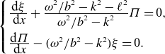 \begin{equation} \left \{\begin{array}{@{}l@{}l} \frac {\displaystyle {\rm d}\xi }{\displaystyle {\,}{\rm d}x} + \frac {\displaystyle \omega ^2/b^2 - k^2 - \ell ^2}{\displaystyle \omega ^2/b^2 - k^2} \varPi = 0 , \\[10pt] \frac {\displaystyle {\rm d} \varPi }{\displaystyle {\,}{\rm d}x} - (\omega ^2/b^2 - k^2) \xi = 0 . \end{array} \right . \end{equation}
The second-order ODE is most convenient for explicit analysis, e.g. of the solutions in the external plasma (where $b = \hat {b} \equiv 1$
), whereas the system of first-order ODEs is most adequate for numerical solution in the internal plasma (where
$b = \hat {b} \equiv 1$
), whereas the system of first-order ODEs is most adequate for numerical solution in the internal plasma (where $b = b(x)$
). Evidently, solution of the BVP by matching the internal to the external solution at
$b = b(x)$
). Evidently, solution of the BVP by matching the internal to the external solution at $|x| = 1$
will involve both. It will be noticed that the first-order system (5.11) for the
$|x| = 1$
will involve both. It will be noticed that the first-order system (5.11) for the $\ell = 0$
fast modes becomes identical to the first-order system (2.11) for the TE modes when the following identifications are made:
$\ell = 0$
fast modes becomes identical to the first-order system (2.11) for the TE modes when the following identifications are made:
 \begin{equation} E \rightarrow v \equiv \partial _t \xi = - {\mathrm{i}} \omega \xi ,\qquad H \rightarrow \varPi , \end{equation}
where $v$
is the velocity perturbation in the
$v$
is the velocity perturbation in the $x$
-direction. This is convenient for checking the numerical procedures. Clearly, these identifications no longer hold for
$x$
-direction. This is convenient for checking the numerical procedures. Clearly, these identifications no longer hold for $\ell \ne 0$
, when the Alfvén waves enter the picture.
$\ell \ne 0$
, when the Alfvén waves enter the picture.
At this point, it should be stressed that the second-order ODE (5.10) for MHD waves in plane geometry is, in fact, a gross simplification of the dynamics of these waves in actual magnetic flux tubes observed in the solar corona. However, for the more realistic cylindrical geometry and arbitrary equilibrium distributions, the analogous equation derived long ago by Hain & Lüst (Reference Hain and Lüst1958), exhibits the same structure with a singular factor in front of the highest derivative (albeit slightly more general, including the singular contributions of the slow magneto-sonic modes). Possible instabilities due to pressure and current contributions are only represented by additional terms in front of the last term, the one multiplying $\xi$
in (5.10). In particular, the fundamental paper by Newcomb (Reference Newcomb1960) on the stability of all diffuse linear pinches is obtained in the limit
$\xi$
in (5.10). In particular, the fundamental paper by Newcomb (Reference Newcomb1960) on the stability of all diffuse linear pinches is obtained in the limit $\omega \rightarrow 0$
of this equation. Hence, as stated previously, the present plane geometry may be considered as sufficiently exemplary to investigate the physical reality of leaky fast magneto-sonic modes in coronal flux tubes.
$\omega \rightarrow 0$
of this equation. Hence, as stated previously, the present plane geometry may be considered as sufficiently exemplary to investigate the physical reality of leaky fast magneto-sonic modes in coronal flux tubes.
There is yet another matter that should be stressed: the innocuously looking elimination of $\xi _y$
from the spectral problem does not have a counterpart in the dielectric problem. In MHD, that variable describes the plasma displacement tangential to the magnetic surfaces, which is the main component of the Alfvén waves, i.e. of the central constituents of MHD spectra! It becomes singular for frequencies
$\xi _y$
from the spectral problem does not have a counterpart in the dielectric problem. In MHD, that variable describes the plasma displacement tangential to the magnetic surfaces, which is the main component of the Alfvén waves, i.e. of the central constituents of MHD spectra! It becomes singular for frequencies $\omega \rightarrow \omega _{\mathrm{A}} = k b(x_{\mathrm{s}})$
at positions
$\omega \rightarrow \omega _{\mathrm{A}} = k b(x_{\mathrm{s}})$
at positions $x = x_{\mathrm{s}}$
, as is evident from the second relation (5.8) for
$x = x_{\mathrm{s}}$
, as is evident from the second relation (5.8) for $\ell = 0$
:
$\ell = 0$
:
 \begin{equation} (\omega ^2/b^2 - k^2) \xi _y = 0 \quad \Rightarrow \quad \xi _y = C \delta (x - x_{\mathrm{s}}) , \end{equation}
whereas the function $\xi _x(x)$
has no influence on this. For
$\xi _x(x)$
has no influence on this. For $\ell \ne 0$
, the algebra becomes a little more involved with Heaviside functions entering the solutions
$\ell \ne 0$
, the algebra becomes a little more involved with Heaviside functions entering the solutions $\xi _x$
of the ODE (5.10), but the resulting component
$\xi _x$
of the ODE (5.10), but the resulting component $\xi _y$
remains the dominant
$\xi _y$
remains the dominant $\delta$
-function contributor.
$\delta$
-function contributor.
The merit of keeping the mode number $\ell$
in the ODE (5.10) is that the genuine Alfvén singularities in the numerator of the term multiplying the second derivative, at
$\ell$
in the ODE (5.10) is that the genuine Alfvén singularities in the numerator of the term multiplying the second derivative, at $\omega = \pm \omega _{\mathrm{A}}(x) \equiv \pm k b(x)$
, are not cancelled by the ‘fake’ fast singularities in the denominator, at
$\omega = \pm \omega _{\mathrm{A}}(x) \equiv \pm k b(x)$
, are not cancelled by the ‘fake’ fast singularities in the denominator, at $\omega = \pm \omega _{\mathrm{f0}}(x) \equiv \pm k_{\mathrm{tot}}{\,}b(x)$
with
$\omega = \pm \omega _{\mathrm{f0}}(x) \equiv \pm k_{\mathrm{tot}}{\,}b(x)$
with $k_{\mathrm{tot}} \equiv \sqrt {k^2 + \ell ^2}$
. The Alfvén singularities produce the continuous Alfvén spectra,
$k_{\mathrm{tot}} \equiv \sqrt {k^2 + \ell ^2}$
. The Alfvén singularities produce the continuous Alfvén spectra,
 \begin{equation} \omega _{\mathrm{A,\,min}} \,\{= k b(1 - \epsilon ) \equiv k \delta \}\, \leqslant \,|\sigma | \leqslant \omega _{\mathrm{A,\,max}} \{= k b(1) \equiv k\}, \end{equation}
corresponding to ‘improper’ eigenfunctions which are singular for the real frequencies $|\sigma | = \omega _{\mathrm{A}}(x_{\mathrm{s}})$
in the range
$|\sigma | = \omega _{\mathrm{A}}(x_{\mathrm{s}})$
in the range $1 - \epsilon \leqslant x_{\mathrm{s}} \leqslant 1$
. The explicit expressions in curly brackets for the boundaries of this continuum are obtained from the choice (3.1) for the phase velocity replacing
$1 - \epsilon \leqslant x_{\mathrm{s}} \leqslant 1$
. The explicit expressions in curly brackets for the boundaries of this continuum are obtained from the choice (3.1) for the phase velocity replacing $v(x)$
by
$v(x)$
by $b(x)$
. The fast apparent singularities
$b(x)$
. The fast apparent singularities $\omega = \pm \omega _{\mathrm{f0}}(x)$
just indicate where the monotonic relation between frequency and oscillations of the eigenfunctions no longer holds (Goedbloed & Sakanaka Reference Goedbloed and Sakanaka1974), although the eigenfunctions themselves remain quadratically integrable. In general, the oscillatory properties of the sub-spectra change at the boundaries of both the singular and the apparently singular frequency regions. Hence, a Sturmian sequence of discrete Alfvén waves could occur for frequencies below the lower edge of the Alfvén continuum,
$\omega = \pm \omega _{\mathrm{f0}}(x)$
just indicate where the monotonic relation between frequency and oscillations of the eigenfunctions no longer holds (Goedbloed & Sakanaka Reference Goedbloed and Sakanaka1974), although the eigenfunctions themselves remain quadratically integrable. In general, the oscillatory properties of the sub-spectra change at the boundaries of both the singular and the apparently singular frequency regions. Hence, a Sturmian sequence of discrete Alfvén waves could occur for frequencies below the lower edge of the Alfvén continuum, $0 \lt |\sigma | \lt \omega _{\mathrm{A,\,min}}$
, and an anti-Sturmian sequence of discrete Alfvén waves above the upper edge,
$0 \lt |\sigma | \lt \omega _{\mathrm{A,\,min}}$
, and an anti-Sturmian sequence of discrete Alfvén waves above the upper edge, $\omega _{\mathrm{A,\,max}} \lt |\sigma | \lt k_{\mathrm{tot}}$
. Because of the extremely simplified present configuration, there are no discrete Alfvén waves in this problem, but only Alfvén continuum modes. However, there is a sequence of discrete fast waves which is Sturmian for
$\omega _{\mathrm{A,\,max}} \lt |\sigma | \lt k_{\mathrm{tot}}$
. Because of the extremely simplified present configuration, there are no discrete Alfvén waves in this problem, but only Alfvén continuum modes. However, there is a sequence of discrete fast waves which is Sturmian for $k_{\mathrm{tot}} \lt |\sigma | \lt \infty$
that would cluster for
$k_{\mathrm{tot}} \lt |\sigma | \lt \infty$
that would cluster for $|\sigma | \rightarrow \infty$
, but only when the external plasma is finite. In the present case, it is replaced by a continuum since the external plasma is assumed to be infinite. In addition, fast discrete modes may occur, and here actually do occur, for
$|\sigma | \rightarrow \infty$
, but only when the external plasma is finite. In the present case, it is replaced by a continuum since the external plasma is assumed to be infinite. In addition, fast discrete modes may occur, and here actually do occur, for $\omega _{\mathrm{A,\,max}} \lt |\sigma | \leqslant k_{\mathrm{tot}}$
. That sequence could connect to an anti-Sturmian sequence of discrete Alfvén waves if those would be permitted (hence, the proof of monotonicIty fails in that frequency range). All this only refers to conservative modes, the leaky ones will be studied in § 6.
$\omega _{\mathrm{A,\,max}} \lt |\sigma | \leqslant k_{\mathrm{tot}}$
. That sequence could connect to an anti-Sturmian sequence of discrete Alfvén waves if those would be permitted (hence, the proof of monotonicIty fails in that frequency range). All this only refers to conservative modes, the leaky ones will be studied in § 6.
Since the Alfvén speed is constant in the external plasma, the two factors in the ODE (5.10) can be extracted from the derivative for $|x| \gt 1$
to yield the external dispersion equation of the Alfvén and fast magneto-sonic modes,
$|x| \gt 1$
to yield the external dispersion equation of the Alfvén and fast magneto-sonic modes,
 \begin{equation} (\omega ^2 - k^2)(\omega ^2 - \hat {q}^2 - k^2 - \ell ^2) = 0 , \end{equation}
where $\hat {q}$
is the mode number in the
$\hat {q}$
is the mode number in the $x$
-direction appearing in the expression for the external variables
$x$
-direction appearing in the expression for the external variables $\hat {\xi }(x)$
and
$\hat {\xi }(x)$
and $\hat {\varPi }(x)$
, analogous to (2.13). Since the first factor exclusively vanishes for real values of
$\hat {\varPi }(x)$
, analogous to (2.13). Since the first factor exclusively vanishes for real values of $\omega$
in the ranges of the Alfvén continua, inversion of the external dispersion equation to produce the relation
$\omega$
in the ranges of the Alfvén continua, inversion of the external dispersion equation to produce the relation $\hat {q} = \hat {q}(\omega )$
needed for the construction of the Spectral Web is nearly the same as in § 2.3 for the TE modes. In particular, the explicit solution (2.14) and figure 2 delineating the different cutoff and propagation regions remain valid, provided that, on the real axis, the crossings at
$\hat {q} = \hat {q}(\omega )$
needed for the construction of the Spectral Web is nearly the same as in § 2.3 for the TE modes. In particular, the explicit solution (2.14) and figure 2 delineating the different cutoff and propagation regions remain valid, provided that, on the real axis, the crossings at $|\sigma | = k$
are replaced by
$|\sigma | = k$
are replaced by $|\sigma | = k_{\mathrm{tot}}$
and the isolated strips
$|\sigma | = k_{\mathrm{tot}}$
and the isolated strips $k \delta \leqslant |\sigma | \leqslant k$
are excluded.
$k \delta \leqslant |\sigma | \leqslant k$
are excluded.
As an aside, the spectral equation (5.10) was studied before in one of the first papers on Alfvén wave heating in tokamaks by Chen & Hasegawa (Reference Chen and Hasegawa1974), extensively described in Section 11.1 of Goedbloed et al. (Reference Goedbloed, Keppens and Poedts2019). As customary for laboratory settings, instead of external fast modes, an external vacuum with exciting electromagnetic waves was assumed. Corresponding to the non-relativistic MHD model, their frequency could be neglected, but they effectively couple to the internal fast waves and then, through wave transformation, to the singular Alfvén waves which would be ‘dissipated’ by continuum damping. Clearly, this mechanism should also work in solar magnetic flux tubes with the present fast external waves as an exciting mechanism. It is also clear now that this requires fast wave frequencies in the cutoff region, where the Alfvén waves are located. The present paper is not concerned with Alfvén wave heating, but with the physics of leaky modes, which occur for fast wave frequencies in the propagating region. As a further aside, it should be mentioned that the replacement of a vacuum magnetic perturbation (customary for fusion experiments) by a plasma with fast magnetosonic waves in the more realistic cylindrical geometry for flux tubes requires the analysis of Bessel or Hankel functions with complex argument, like ${\mathrm{J}}_m(\sqrt {\omega ^2 - k^2}{\,}r)$
. This complication is avoided here by exploiting a plane slab geometry permitting straightforward inversion of the external dispersion equation.
${\mathrm{J}}_m(\sqrt {\omega ^2 - k^2}{\,}r)$
. This complication is avoided here by exploiting a plane slab geometry permitting straightforward inversion of the external dispersion equation.
5.3. Boundary value problem for Alfvén–fast magnetosonic waves
Analogous to § 2.3 on the TE modes, the internal, numerical solutions of the ODEs (5.11) for the Alfvén–fast magnetosonic spectral problem are written as
 \begin{equation} \xi = \xi (x) ,\quad \varPi = \varPi (x) \qquad {(|x| \leqslant 1)} , \end{equation}
whereas the same ODEs, for $b(x) = \hat {b} \equiv 1$
and eliminating
$b(x) = \hat {b} \equiv 1$
and eliminating $\omega$
with the external dispersion equation (5.15), provide the explicit external solutions:
$\omega$
with the external dispersion equation (5.15), provide the explicit external solutions:
 \begin{equation} \hat {\xi }(x) = \hat {\alpha }{\mathrm{e}}^{{\mathrm{i}}\hat {q}x} + \hat {\beta }{\mathrm{e}}^{-{\mathrm{i}} \hat {q}x} ,\quad \hat {\varPi }(x) = - {\mathrm{i}}\hat {q} \big(1 + \ell ^2/\hat {q}^2\big)\big(\hat {\alpha }{\mathrm{e}}^{{\mathrm{i}}\hat {q}x} - \hat {\beta }{\mathrm{e}}^{-{\mathrm{i}} \hat {q}x}\big) \qquad {(|x| \gt 1)} . \end{equation}
The boundary conditions to match these solutions are the same as (2.23)–(2.25), of course with proper changes of the variables:
 \begin{align} \text{(a) at }|x| & = 0:\; \xi (0) = 0 \; (\mathrm{odd\ modes}) \quad \text{or}\quad \varPi (0) = 0 \; (\mathrm{even\ modes}) ,\\[-10pt]\nonumber\end{align}
 \begin{align} \text{(b) at }|x| & = 1: \; \xi (1) = \hat {\xi }(1) \quad \text{and}\quad \varPi (1) = \hat {\varPi }(1) ,\\[-10pt]\nonumber \end{align}
 \begin{align}\text{(c) at }|x| & \rightarrow \infty , \left \{\begin{array}{@{}l@{}l} (\mathrm{c}1)\ \mathrm{CNMs}: \ \hat {\alpha } = 0 \ {(\text{for }|\sigma | \lt k_{\mathrm{tot}})},\quad |\hat {\alpha }| = |\hat {\beta }| \ {(\text{for }|\sigma | \geqslant k_{\mathrm{tot}})},\\[3pt] (\mathrm{c}2)\ {\mathrm{Leaky\, modes}}: \ \hat {\beta } = 0. \end{array} \right .\end{align}
Here, the auxiliary parameter $k_{\mathrm{tot}} \equiv \sqrt {k^2 + \ell ^2}$
marks the cutoff boundary, and the leaky fast magnetosonic modes are not indicated as QNMs since it is yet to be proved that this terminology would be appropriate for these modes.
$k_{\mathrm{tot}} \equiv \sqrt {k^2 + \ell ^2}$
marks the cutoff boundary, and the leaky fast magnetosonic modes are not indicated as QNMs since it is yet to be proved that this terminology would be appropriate for these modes.
5.4. Spectral Web for magnetohydrodynamic waves in magnetised plasmas
Justification of the above-mentioned boundary conditions and construction of the Spectral Web for this case requires a quantity corresponding to the Poynting flux of § 2.4. For this purpose, the potential energy $W$
of the perturbations will be chosen. It is a quadratic function of the displacement vector
$W$
of the perturbations will be chosen. It is a quadratic function of the displacement vector $\boldsymbol{\xi }$
appearing in the force operator
$\boldsymbol{\xi }$
appearing in the force operator $\mathbf{F}$
, which has been shown to be self-adjoint by rather cumbersome vector operations converting the original volume integral into a symmetric volume integral over the plasma complemented with a surface integral over the outer boundary. Since all this is standard theory, we just adapt the well-known expression to our system of the two plasmas by splitting the complete volume integral into two parts, where the crucial new construct is an additional surface integral over the separating boundary
$\mathbf{F}$
, which has been shown to be self-adjoint by rather cumbersome vector operations converting the original volume integral into a symmetric volume integral over the plasma complemented with a surface integral over the outer boundary. Since all this is standard theory, we just adapt the well-known expression to our system of the two plasmas by splitting the complete volume integral into two parts, where the crucial new construct is an additional surface integral over the separating boundary $S_1$
(at
$S_1$
(at $|x| = 1$
for the present case):
$|x| = 1$
for the present case):
 \begin{eqnarray} W &\,\equiv\, & - {\frac {1}{2}} \int \boldsymbol{\xi }^* \boldsymbol{\cdot }\mathbf{F}(\boldsymbol{\xi }) {\,}{\rm d}V \nonumber \\[6pt] &\,=\,& {\frac {1}{2}} \int \mathbf{Q}\boldsymbol{\cdot }\mathbf{Q}^* {\rm d}V - {\frac {1}{2}} \int \boldsymbol{\xi }^*\!\boldsymbol{\cdot }\mathbf{n} \,\lbrack \!\lbrack \varPi \rbrack \!\rbrack {\,}{\rm d}S_1 + {\frac {1}{2}} \int \hat {\mathbf{Q}}\boldsymbol{\cdot }\hat {\mathbf{Q}}^* {\rm d}\hat {V} + \int \hat {\boldsymbol{\xi }}^*\!\boldsymbol{\cdot }\mathbf{n} \hat {\varPi } {\,}{\rm d}\hat {S} .\nonumber\\ \end{eqnarray}
The volume integrals only contain the magnetic field perturbations $\mathbf{Q}$
and
$\mathbf{Q}$
and $\hat {\mathbf{Q}}$
since the equilibrium current and pressure are assumed to vanish. The surface integrals are completely general. They manifest the surprising property of ideal MHD that all perturbations can be reduced to the two variables
$\hat {\mathbf{Q}}$
since the equilibrium current and pressure are assumed to vanish. The surface integrals are completely general. They manifest the surprising property of ideal MHD that all perturbations can be reduced to the two variables $\xi \equiv \boldsymbol{\xi } \boldsymbol{\cdot }\mathbf{n}$
and
$\xi \equiv \boldsymbol{\xi } \boldsymbol{\cdot }\mathbf{n}$
and $\varPi$
which are propagated from magnetic surface to magnetic surface by the pertinent ODEs or partial differential equations. The second surface integral imports the outer BC, which may be situated at infinity.
$\varPi$
which are propagated from magnetic surface to magnetic surface by the pertinent ODEs or partial differential equations. The second surface integral imports the outer BC, which may be situated at infinity.
Corresponding to the definition (2.29) of the complementary Poynting flux, averaged over a unit surface area, the first surface integral is the complementary energy,
 \begin{equation} W_{\mathrm{com}} \equiv - \frac {1}{2 L_y L_z} \int _{-L_y}^{L_y} \int _{-L_z}^{L_z} \lbrack \!\lbrack {\varPi }\rbrack \!\rbrack \xi ^*{\,}{\rm d}y{\,}{\rm d}z = - {\frac {1}{2}} \xi ^*(1) \lbrack \!\lbrack {\varPi (1)}\rbrack \!\rbrack . \end{equation}
It will be used to construct the Spectral Web for arbitrary complex values of $\omega$
by computing internal solutions satisfying the BCs (5.18), external solutions satisfying either one of the two BCs (5.20) and matching them by imposing continuity of
$\omega$
by computing internal solutions satisfying the BCs (5.18), external solutions satisfying either one of the two BCs (5.20) and matching them by imposing continuity of $\xi$
at
$\xi$
at $x = 1$
. The second BC (5.19), continuity of
$x = 1$
. The second BC (5.19), continuity of $\varPi$
, will then not be satisfied in general, except for the wanted eigenvalues. The last term of (5.21), the surface integral over the boundary at infinity, represents the energy that is being lost there (for the leaky modes) or not (for the conservative modes). The Spectral Web method to construct these two types of modes is completely analogous to that used in § 2.4 to construct the spectra for the conservative and leaky TE modes so that we can now proceed to the similar computation for the Alfvén and fast magneto-sonic modes.
$\varPi$
, will then not be satisfied in general, except for the wanted eigenvalues. The last term of (5.21), the surface integral over the boundary at infinity, represents the energy that is being lost there (for the leaky modes) or not (for the conservative modes). The Spectral Web method to construct these two types of modes is completely analogous to that used in § 2.4 to construct the spectra for the conservative and leaky TE modes so that we can now proceed to the similar computation for the Alfvén and fast magneto-sonic modes.
6. Spectra of conservative and leaky Alfvén–fast modes
6.1. Preliminaries
Analogous to § 3.1 for the electromagnetic waves, we exploit the distribution (3.1), with the same two parameters $\epsilon$
and
$\epsilon$
and $\delta$
determining size and strength of the inhomogeneity, whereas the phase velocity
$\delta$
determining size and strength of the inhomogeneity, whereas the phase velocity $v(x)$
is replaced by the Alfvén velocity
$v(x)$
is replaced by the Alfvén velocity $b(x)$
. Now, an additional wavenumber
$b(x)$
. Now, an additional wavenumber $\ell$
in the
$\ell$
in the $y$
-direction enters so that the total wavenumber, tangential to the magnetic surfaces, becomes
$y$
-direction enters so that the total wavenumber, tangential to the magnetic surfaces, becomes $k_{\mathrm{tot}} \equiv \sqrt {k^2 + \ell ^2}$
. Hence, in contrast to the three-parameter numerical code DLEAK (employed in § 3) for the EM waves in dielectric media, the numerical code CLEAK (employed in this section) for MHD waves in coronal loops contains four free parameters, viz.
$k_{\mathrm{tot}} \equiv \sqrt {k^2 + \ell ^2}$
. Hence, in contrast to the three-parameter numerical code DLEAK (employed in § 3) for the EM waves in dielectric media, the numerical code CLEAK (employed in this section) for MHD waves in coronal loops contains four free parameters, viz. $\epsilon$
,
$\epsilon$
, $\delta$
,
$\delta$
, $k$
and
$k$
and $\ell$
. The value of
$\ell$
. The value of $\epsilon$
will now be chosen larger to make the configuration for coronal loops one step more realistic. The values of the other parameters will be chosen largely for the purpose of illustration of the spectral characteristics since it is obvious that the configuration is a ‘caricature’ anyway of the actual magnetic loops that are observed in the solar corona. Nevertheless, the calculation is valuable because it exhibits the main features of the intricate interplay of fast and Alfvén waves that recur in more realistic configurations.
$\epsilon$
will now be chosen larger to make the configuration for coronal loops one step more realistic. The values of the other parameters will be chosen largely for the purpose of illustration of the spectral characteristics since it is obvious that the configuration is a ‘caricature’ anyway of the actual magnetic loops that are observed in the solar corona. Nevertheless, the calculation is valuable because it exhibits the main features of the intricate interplay of fast and Alfvén waves that recur in more realistic configurations.
Recall that the ‘wavenumber’ $q$
in the direction of inhomogeneity is not a valid quantum number for the interior region
$q$
in the direction of inhomogeneity is not a valid quantum number for the interior region $|x| \leqslant 1$
. Its local value is just a result of the numerical solution of the pertinent ODEs. The wavenumber
$|x| \leqslant 1$
. Its local value is just a result of the numerical solution of the pertinent ODEs. The wavenumber $\hat {q}$
for the external region
$\hat {q}$
for the external region $|x| \gt 1$
is a valid quantum number though, determined by the inverse
$|x| \gt 1$
is a valid quantum number though, determined by the inverse $\hat {q}(\omega )$
of the fast wave dispersion equation (5.15). The Spectral Web method hinges on computing the solution paths and the conjugate paths for prescribed complex values of
$\hat {q}(\omega )$
of the fast wave dispersion equation (5.15). The Spectral Web method hinges on computing the solution paths and the conjugate paths for prescribed complex values of $\omega$
. Hence, it is very fortunate that this inversion can be performed algebraically for this configuration, see (2.14) and figure 2 with
$\omega$
. Hence, it is very fortunate that this inversion can be performed algebraically for this configuration, see (2.14) and figure 2 with $k$
replaced by
$k$
replaced by $k_{\mathrm{tot}}$
. Generalisation to cylindrical or more general geometries would be more complicated but, as mentioned at the end of § 3.4, the external solution could then be obtained with the same numerical integration method as exploited for the interior region, i.e. for prescribed values of
$k_{\mathrm{tot}}$
. Generalisation to cylindrical or more general geometries would be more complicated but, as mentioned at the end of § 3.4, the external solution could then be obtained with the same numerical integration method as exploited for the interior region, i.e. for prescribed values of $\omega$
. With the speed and accuracy of present numerical solvers, one needs not to bother anymore about computing zeros of Hankel functions.
$\omega$
. With the speed and accuracy of present numerical solvers, one needs not to bother anymore about computing zeros of Hankel functions.
6.2. Conservative Alfvén–fast modes
Representative spectra of the conservative normal modes, i.e. the regular MHD waves in a coronal magnetic flux tube, are depicted in figure 7. Compared with the EM spectra depicted in figures 3 and 4, there are now the additional contributions of the Alfvén waves in the MHD spectra of figures 7 and 8. To exhibit those most clearly, only the positive frequency parts of the spectra are dsplayed.
Spectra of conservative normal modes, i.e. regular MHD waves in a coronal magnetic flux tube as depicted in figure 1: (a) even modes; (b) odd modes. The parameters are $\epsilon = 0.2$
,
$\epsilon = 0.2$
, $\delta = 0.25$
,
$\delta = 0.25$
, $k = \ell = 5.0$
. The modes
$k = \ell = 5.0$
. The modes $n = 1 \boldsymbol{\cdot}s 6$
, or
$n = 1 \boldsymbol{\cdot}s 6$
, or $n = 1, \ldots, 5$
, have been ‘swallowed’ by the Alfvén continua. The remaining modes
$n = 1, \ldots, 5$
, have been ‘swallowed’ by the Alfvén continua. The remaining modes $n = 7, 8, 9$
, or
$n = 7, 8, 9$
, or $n = 6, 7, 8$
, refer to discrete bound modes which, for
$n = 6, 7, 8$
, refer to discrete bound modes which, for $|\sigma | \geqslant k_{\mathrm{tot}}$
, continuously connect to the continua of finite amplitude standing fast waves.
$|\sigma | \geqslant k_{\mathrm{tot}}$
, continuously connect to the continua of finite amplitude standing fast waves.
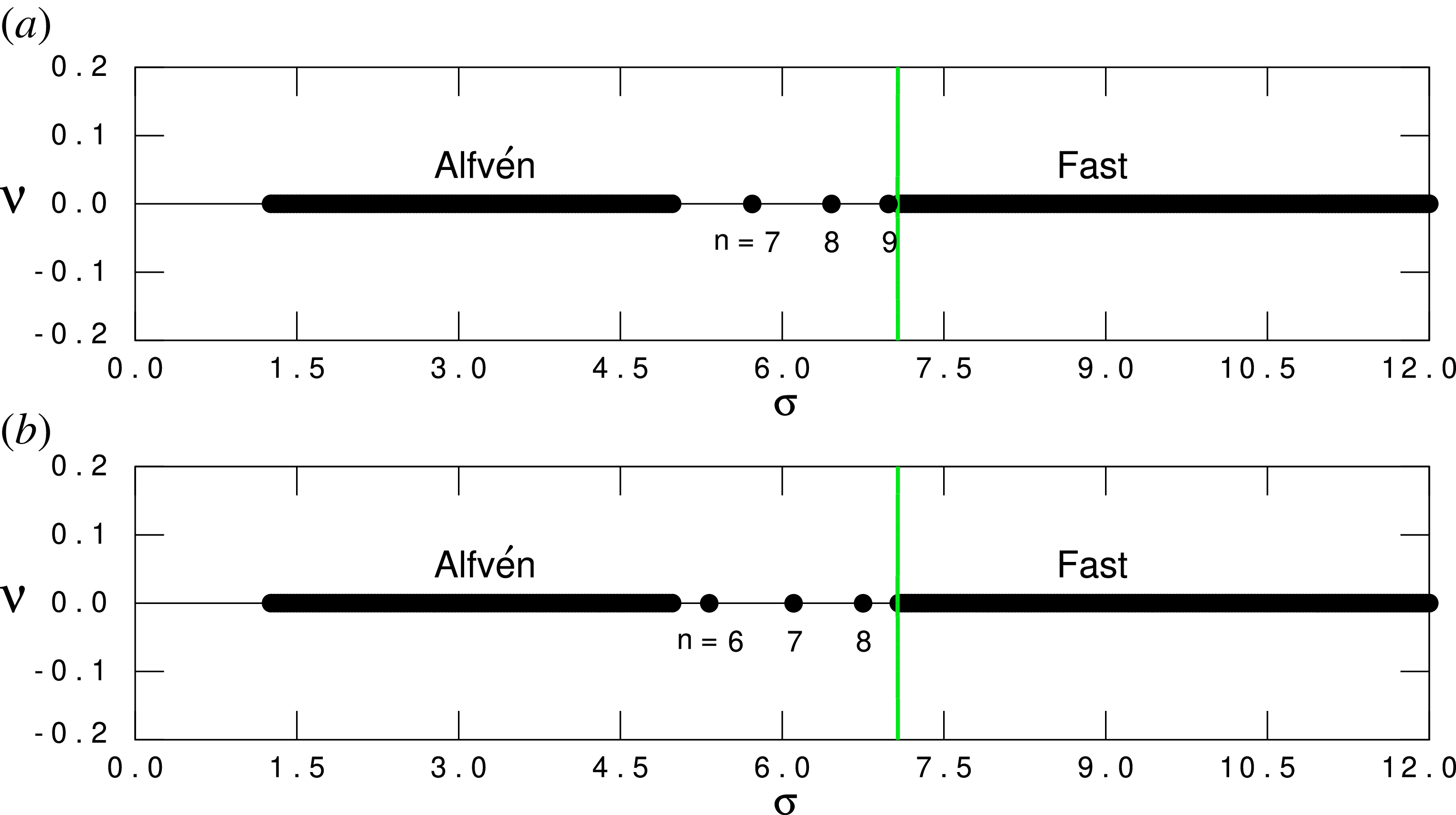
Figure 7 Long description
Two line graphs depict spectra of conservative normal modes in a coronal magnetic flux tube. The x-axis represents the variable sigma ranging from 0.0 to 12.0, and the y-axis represents the variable V ranging from -0.2 to 0.2. The first graph (a) shows even modes, while the second graph (b) shows odd modes. Both graphs feature regions labeled Alfven and Fast, with specific modes marked by black dots. The modes n equals 7 or 9 in graph (a) and n equals 6 or 8 in graph (b) have been swallowed by the Alfven continua. The remaining modes n equals 8 or 9 in graph (a) and n equals 7 or 8 in graph (b) refer to discrete bound modes which, for sigma equals 7.5, continuously connect to the continua of finite amplitude standing fast waves. A green vertical line at sigma equals 7.5 highlights a specific point of interest in both graphs.
To understand the fundamental difference between the EM waves of figure 3 and the MHD waves of figure 7, it may be helpful to recall the elementary properties of Alfvén and fast waves for homogeneous plasmas. In that case, since $\xi _x \sim \xi _y \sim \exp ({\mathrm{i}} q x)$
, the ODEs (5.8) become an algebraic system having, not surprisingly, the discriminant (5.15) with
$\xi _x \sim \xi _y \sim \exp ({\mathrm{i}} q x)$
, the ODEs (5.8) become an algebraic system having, not surprisingly, the discriminant (5.15) with $\hat {q}$
replaced by
$\hat {q}$
replaced by $q$
. The solutions are
$q$
. The solutions are
 \begin{align} &- \mathrm{degenerate\ Alfv}{\acute{\mathrm{e}}}\mathrm{n\ waves}\ \text{at}\ \omega ^2/b^2 = k^2, \text{ with } \,\boldsymbol{\xi }_{\mathrm{A}} \perp \mathbf{k}_\perp \equiv (q, \ell , 0),\\[-10pt]\nonumber \end{align}
 \begin{align} &- \mathrm{fast\ magneto\text{-}sonic\ waves} \text{ at } \,\omega ^2/b^2 = k_{\mathrm{tot}}^2 + q^2, \text{ with }\,\boldsymbol{\xi }_{\mathrm{F}} \parallel \mathbf{k}_\perp . \end{align}
For a finite box, $q$
becomes quantised and the fast mode spectrum becomes a discrete set of eigenvalues starting at
$q$
becomes quantised and the fast mode spectrum becomes a discrete set of eigenvalues starting at $\omega ^2/b^2 = k_{\mathrm{tot}}^2$
. If the box is infinite, the fast spectrum becomes a continuum. For the present inhomogeneous case (extended with an external region with wave number
$\omega ^2/b^2 = k_{\mathrm{tot}}^2$
. If the box is infinite, the fast spectrum becomes a continuum. For the present inhomogeneous case (extended with an external region with wave number $\hat {q}$
), the local internal wavenumber
$\hat {q}$
), the local internal wavenumber $q(x)$
may become imaginary, giving rise to an extension with bound fast waves in the cutoff region
$q(x)$
may become imaginary, giving rise to an extension with bound fast waves in the cutoff region $0 \lt |\sigma |/b \lt k_{\mathrm{tot}}$
. With an inhomogeneous internal region, the degenerate Alfvén spectrum also becomes a continuum with frequencies given by (5.14). (Keep in mind though that this continuum is of a completely different nature than the fast continuum.) A good fraction of the bound fast waves are ‘swallowed’ by the Alfvén continuum. Whereas for
$0 \lt |\sigma |/b \lt k_{\mathrm{tot}}$
. With an inhomogeneous internal region, the degenerate Alfvén spectrum also becomes a continuum with frequencies given by (5.14). (Keep in mind though that this continuum is of a completely different nature than the fast continuum.) A good fraction of the bound fast waves are ‘swallowed’ by the Alfvén continuum. Whereas for $\ell = 0$
, the fast mode spectrum is governed by the same ODE (5.10) for
$\ell = 0$
, the fast mode spectrum is governed by the same ODE (5.10) for $\xi _x$
as the ODE (2.10) for
$\xi _x$
as the ODE (2.10) for $E_y$
governing the TE mode spectrum, it is obvious that this analogy completely breaks down for
$E_y$
governing the TE mode spectrum, it is obvious that this analogy completely breaks down for $\ell \ne 0$
since EM waves do not have the similar counterpart of Alfvén waves. All this is clearly demonstrated by figure 7.
$\ell \ne 0$
since EM waves do not have the similar counterpart of Alfvén waves. All this is clearly demonstrated by figure 7.
Spectra of leaky MHD waves in a coronal magnetic flux tube as depicted in figure 1: (a) even modes; (b) odd modes. The parameters are the same as in figure 7. Again, the lower modes have been ‘swallowed’ by the Alfvén continua. The remaining modes $n = 7, 8$
or
$n = 7, 8$
or $n = 6, 7$
refer to discrete unbound modes which, for
$n = 6, 7$
refer to discrete unbound modes which, for $|\sigma | \geqslant k_{\mathrm{tot}}$
, discontinuously ‘connect’ onto the discrete spectra of propagating fast waves with exponentially growing amplitudes for
$|\sigma | \geqslant k_{\mathrm{tot}}$
, discontinuously ‘connect’ onto the discrete spectra of propagating fast waves with exponentially growing amplitudes for $|x| \rightarrow \infty$
.
$|x| \rightarrow \infty$
.
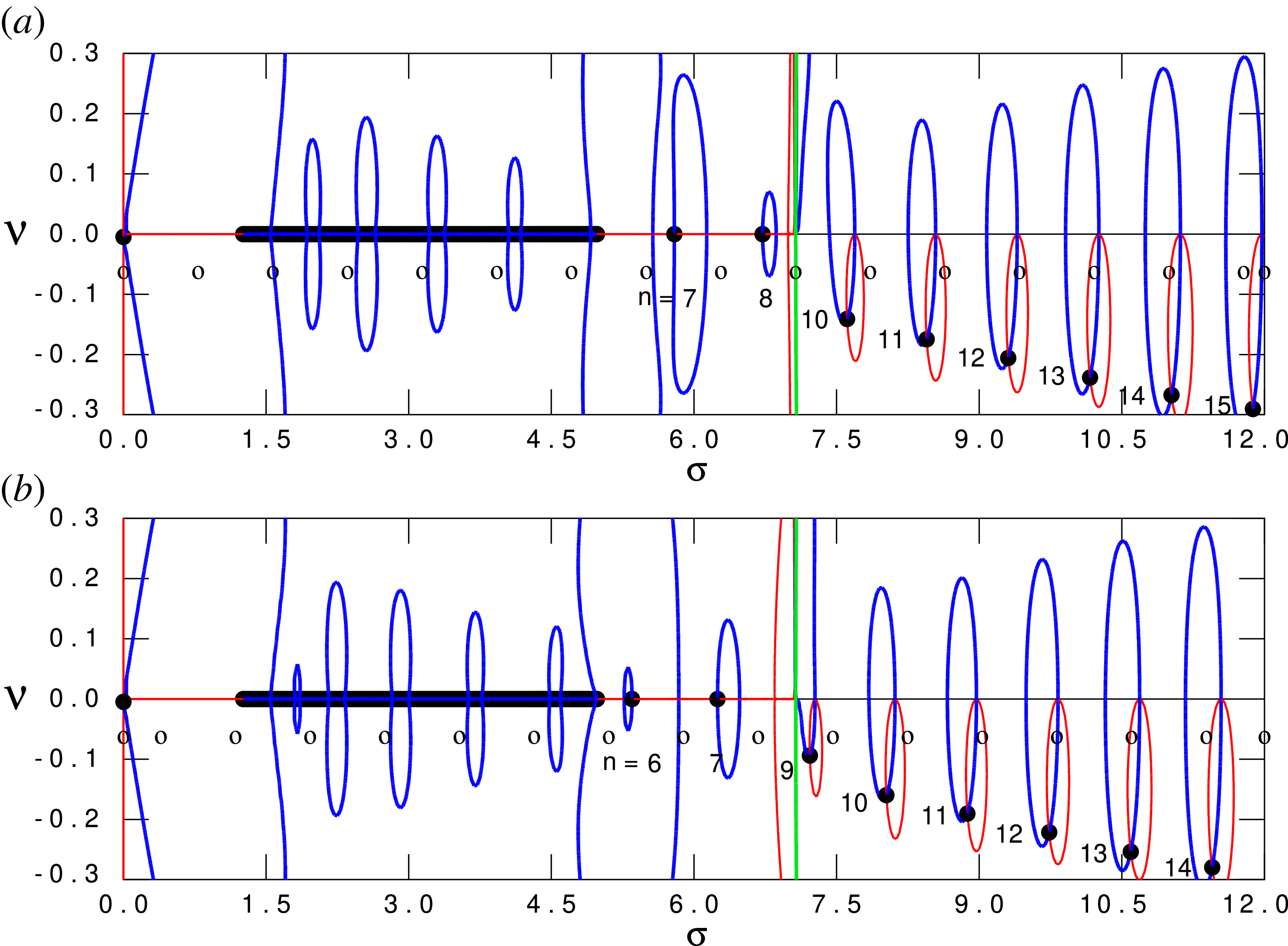
Figure 8 Long description
The image contains two graphs labeled (a) and (b), representing the spectra of leaky magnetohydrodynamic (MHD) waves in a coronal magnetic flux tube. Graph (a) shows even modes, while graph (b) shows odd modes. Both graphs share the same parameters as a previous figure, likely figure 7. The x-axis represents the variable sigma, ranging from 0.0 to 12.0, and the y-axis represents the variable nu, ranging from -0.3 to 0.3. The graphs feature blue oscillating lines indicating the spectra, with specific points marked by black and white circles. Red ellipses highlight certain regions of interest. The lower modes are noted to be swallowed by the Alfven continua, and the remaining modes refer to discrete unbound modes that connect onto the discrete spectra of propagating fast waves with exponentially growing amplitudes for certain values of sigma. The graphs illustrate the complex behavior of these waves under different conditions, showing how they transition and interact within the specified parameter range.
6.3. Leaky Alfvén–fast modes
Representative spectra of the leaky MHD waves in a coronal magnetic flux tube are depicted in figure 8. The apparent similarity (in particular, in the propagating region) between the conservative TE mode spectra and the conservative MHD mode spectra, depicted in figures 3 and 7, and between the leaky mode spectra depicted in figures 4 and 8, demands a careful analysis though. In figure 8, a good fraction of the leaky MHD modes in the cutoff region is again ‘swallowed’ by the Alfvén continuum, but the two leaky modes close to $\omega = 0$
, at
$\omega = 0$
, at $\nu = 4.7048\times 10^{-3}$
(even modes) and at
$\nu = 4.7048\times 10^{-3}$
(even modes) and at $\sigma = 4.7070\times 10^{-3}$
(odd modes), are obviously not affected by the Alfvén continuum. From (5.10), these ‘solutions’ already grow explosively as
$\sigma = 4.7070\times 10^{-3}$
(odd modes), are obviously not affected by the Alfvén continuum. From (5.10), these ‘solutions’ already grow explosively as $\xi \sim \exp {(k_{\mathrm{tot}} |x|)}$
close to
$\xi \sim \exp {(k_{\mathrm{tot}} |x|)}$
close to $|x| = 0$
so that they formally belong to the leaky mode variety. If we label them by
$|x| = 0$
so that they formally belong to the leaky mode variety. If we label them by $n = 1$
, it already becomes complicated to recognise the connection with the other ‘eigenvalues’ of the leaky modes in the cutoff region. For the particular choice of the parameters
$n = 1$
, it already becomes complicated to recognise the connection with the other ‘eigenvalues’ of the leaky modes in the cutoff region. For the particular choice of the parameters $k$
and
$k$
and $\ell$
in figure 8, only two have remained, viz.
$\ell$
in figure 8, only two have remained, viz. $n = 7, 8$
(even modes) and
$n = 7, 8$
(even modes) and $n = 6, 7$
(odd modes). For MHD, not much remains of the alternating sequences of conservative and leaky modes illustrated in table 1(a), i.e. not much of a spectral structure if one wishes to develop ‘coronal seismology’ based on leaky fast modes! Here, we have just skipped the smaller mode labels and continued counting beyond the Alfvén continuum by following the same procedure as for the leaky TE modes depicted in figure 4, viz. by counting the zeros of the real part of the ‘eigenfunctions’ on the internal part
$n = 6, 7$
(odd modes). For MHD, not much remains of the alternating sequences of conservative and leaky modes illustrated in table 1(a), i.e. not much of a spectral structure if one wishes to develop ‘coronal seismology’ based on leaky fast modes! Here, we have just skipped the smaller mode labels and continued counting beyond the Alfvén continuum by following the same procedure as for the leaky TE modes depicted in figure 4, viz. by counting the zeros of the real part of the ‘eigenfunctions’ on the internal part $|x| \leqslant 1$
of the configuration.
$|x| \leqslant 1$
of the configuration.
In the propagating region, this counting procedure becomes even more dubious. The zeros of the real parts of the ‘eigenfunctions’ simply jump one digit, whereas the imaginary parts do not exhibit this jump (in contrast to the leaky TE mode spectra depicted in figure 4, where the number of zeros of both the real and the imaginary parts is just continuous). This counting anomaly appears to be connected with a more serious shortcoming of the leaky MHD spectrum in the propagating region depicted in figure 8. Whereas the separate QNM ‘eigenvalues’ of the electromagnetic problem shown in figure 4 are connected by the solution path (the red curve), which justifies the counting procedure based on the monotonicity theorems along the Spectral Web paths proved earlier (Goedbloed Reference Goedbloed2018), no such connection exists in the MHD problem! In contrast, a blow up of the spectrum shows that both paths of the Spectral Web are ‘blocked’ at the cutoff frequency $\sigma = k_{\mathrm{tot}}$
, where the solution path (red) starts to wind about the cutoff curve (green) and then connects onto a conjugate path (blue) which abruptly ends in the propagating region, without providing a connection between the ‘eigenvalues’ of the leaky mode sequence. Each one of them is found at the intersection of a closed loop of the solution path and a similar closed loop of the conjugate path: a beautiful structure, mathematically correct but the connection to the quadratic forms of a physically meaningful spectral theory is questionable. This brings us to the subject of the next section.
$\sigma = k_{\mathrm{tot}}$
, where the solution path (red) starts to wind about the cutoff curve (green) and then connects onto a conjugate path (blue) which abruptly ends in the propagating region, without providing a connection between the ‘eigenvalues’ of the leaky mode sequence. Each one of them is found at the intersection of a closed loop of the solution path and a similar closed loop of the conjugate path: a beautiful structure, mathematically correct but the connection to the quadratic forms of a physically meaningful spectral theory is questionable. This brings us to the subject of the next section.
CNM eigenfunctions corresponding to the spectrum depicted in figure 7(a) for the even modes: (a) a discrete bound mode with $n = 8$
and
$n = 8$
and $\sigma = 6.4563$
on the interval
$\sigma = 6.4563$
on the interval $(0, 8.0)$
; (b) a ‘propagating’ continuum mode with the arbitrary choice
$(0, 8.0)$
; (b) a ‘propagating’ continuum mode with the arbitrary choice $\sigma = 9.0$
of the improper eigenvalue on the same interval. The phase velocity profile
$\sigma = 9.0$
of the improper eigenvalue on the same interval. The phase velocity profile $b(x)$
for this interval is depicted above the eigenfunctions. The parameters
$b(x)$
for this interval is depicted above the eigenfunctions. The parameters $\delta$
,
$\delta$
, $\epsilon$
and
$\epsilon$
and $k$
are the same as in figure 7.
$k$
are the same as in figure 7.
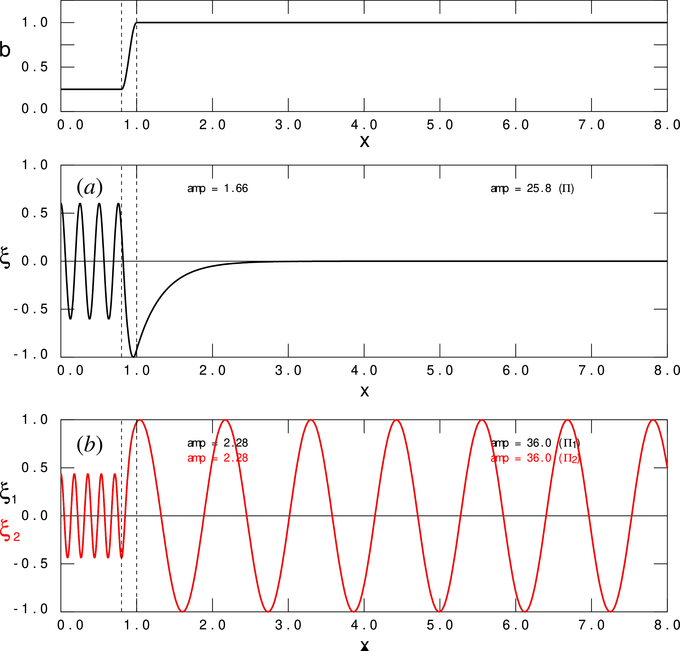
Figure 9 Long description
The image contains three graphs. The top graph shows a phase velocity profile over an interval from 0 to 8 on the x-axis. The middle graph, labeled (a), depicts a discrete bound mode with specific parameters on the same interval. The bottom graph, labeled (b), illustrates a propagating continuum mode with an arbitrary choice of improper eigenvalue over the same interval. The phase velocity profile is shown above the eigenfunctions in the top graph. The parameters and values are consistent with those in figure 7. The graphs are aligned vertically, with the top graph providing context for the middle and bottom graphs. The middle graph shows a bound mode with oscillations that stabilize around 1.0 on the x-axis. The bottom graph displays a continuum mode with varying amplitudes and oscillations. All values are approximated.
7. Attempt to regularise the leaky fast MHD modes
Next, the excitation of the MHD spectrum of Alfvén and fast waves in the solution of the initial value problem needs to be discussed, in analogy with § 4 for the electromagnetic problem. The algebra of § 4.1 for the corresponding MHD problem can be skipped because it is identical. One only has to replace the variable $E(x)$
, satisfying the ODE (2.10) by the variable
$E(x)$
, satisfying the ODE (2.10) by the variable $\xi (x)$
, satisfying the ODE (5.10), and the associated variables
$\xi (x)$
, satisfying the ODE (5.10), and the associated variables $H(x)$
and
$H(x)$
and $\varPi (x)$
according to the scheme (5.12).
$\varPi (x)$
according to the scheme (5.12).
Hence, it appears to remain to derive orthogonality and normalisation relations justifying the use of leaky fast modes in the solution of an initial value problem for coronal magnetic flux tubes, in the same way as in § 4.2 for TE modes in dielectric media. To that end, we start from the MHD time evolution equations in the primitive first-order variables $\mathbf{v}$
and
$\mathbf{v}$
and $\mathbf{Q}$
, since the perturbations of
$\mathbf{Q}$
, since the perturbations of $\rho$
and
$\rho$
and $p$
do not contribute in this problem:
$p$
do not contribute in this problem:
 \begin{equation} \rho \frac {\partial \mathbf{v}}{\partial t} = - \mathbf{B} \times (\boldsymbol{\nabla }\times \mathbf{Q}) ,\qquad \frac {\partial \mathbf{Q}}{\partial t} = - \boldsymbol{\nabla }\times (\mathbf{B} \times \mathbf{v}) . \end{equation}
These equations are to be considered as the counterpart of the basic equations (2.3) for the electrodynamical variables $\mathbf{E}$
and
$\mathbf{E}$
and $\mathbf{H}$
resulting in (4.16) and (4.17) of § 4.2. Similarly, we here consider two modes satisfying the equations (7.1) for the frequencies
$\mathbf{H}$
resulting in (4.16) and (4.17) of § 4.2. Similarly, we here consider two modes satisfying the equations (7.1) for the frequencies $\omega _n$
and
$\omega _n$
and $\omega _m$
:
$\omega _m$
:
 \begin{eqnarray} - {\mathrm{i}}(\omega _n/b^2) \mathbf{v}_n &=& - \mathbf{B} \times (\boldsymbol{\nabla }\times \mathbf{Q}_n), \quad - {\mathrm{i}}\omega _n \mathbf{Q}_n \,\,= - \boldsymbol{\nabla }\times (\mathbf{B} \times \mathbf{v}_n), \end{eqnarray}
 \begin{eqnarray} - {\mathrm{i}}(\omega _m/b^2) \mathbf{v}_m &=& - \mathbf{B} \times (\boldsymbol{\nabla }\times \mathbf{Q}_m), \quad - {\mathrm{i}}\omega _m \mathbf{Q} _m = - \boldsymbol{\nabla }\times (\mathbf{B} \times \mathbf{v}_m). \end{eqnarray}
Quadratic forms are constructed from these equations according to the same scheme as exploited to get (4.19), where now the Alfvén speed $b \equiv B/\sqrt {\rho }$
will enter by dividing
$b \equiv B/\sqrt {\rho }$
will enter by dividing $\mathbf{B}$
and
$\mathbf{B}$
and $\mathbf{Q}$
by the constant value
$\mathbf{Q}$
by the constant value $B$
of the background magnetic field,
$B$
of the background magnetic field,
 \begin{equation} \int _\varOmega \{[\text{(7.2)}(\mathit{a}) \boldsymbol{\cdot }\mathbf{v}_m - \text{(7.3)}(\mathit{a}) \boldsymbol{\cdot }\mathbf{v}_n] \pm [\text{(7.2)}(\mathit{b}) \boldsymbol{\cdot }\mathbf{Q}_m - \text{(7.3)}(\mathit{b}) \boldsymbol{\cdot }\mathbf{Q}_n]\} {\,}{\rm d}V . \end{equation}
This yields two quadratic forms, analogous to the electromagnetic problem:
 \begin{eqnarray} && - {\mathrm{i}} (\omega _n - \omega _m) \int _\varOmega \!\big (\mathbf{v}_n\boldsymbol{\cdot }\mathbf{v}_m/b^2 \pm \mathbf{Q}_n\boldsymbol{\cdot }\mathbf{Q}_m\big ) {\rm d}V \nonumber \\[2pt] &&\qquad = \int _\varOmega [{-} \mathbf{v}_m \boldsymbol{\cdot }\big (\mathbf{B} \times (\boldsymbol{\nabla }\times \mathbf{Q}_n)\big ) + \mathbf{v}_n \boldsymbol{\cdot }(\mathbf{B} \times (\boldsymbol{\nabla }\times \mathbf{Q}_m))] {\rm d}V \nonumber \\[2pt] &&\qquad \qquad \qquad \pm \int _\varOmega [{-} \mathbf{Q}_m \boldsymbol{\cdot }(\boldsymbol{\nabla }\times (\mathbf{B} \times \mathbf{v}_n)) + \mathbf{Q}_n \boldsymbol{\cdot }(\boldsymbol{\nabla }\times (\mathbf{B} \times \mathbf{v}_m))] {\rm d}V \nonumber \\[2pt] &&\qquad = - (1 \pm 1) \int _\varOmega [\mathbf{Q}_n\boldsymbol{\cdot }\mathbf{R}_m - \mathbf{Q}_m\boldsymbol{\cdot }\mathbf{R}_n] {\rm d}V - \int _\varSigma [\mathbf{B}\boldsymbol{\cdot }\mathbf{Q}_n \mathbf{v}_m - \mathbf{B}\boldsymbol{\cdot }\mathbf{Q}_m \mathbf{v}_n] \boldsymbol{\cdot }\mathbf{n} {\rm d}S \nonumber \\[2pt] &&\qquad \equiv - (1 \pm 1){\mathrm{i}}(\omega _n - \omega _m) \int _\varOmega \mathbf{Q}_n\boldsymbol{\cdot }\mathbf{Q}_m {\rm d}V - \int _\varSigma [\varPi _n \mathbf{v}_m - \varPi _m \mathbf{v}_n] \boldsymbol{\cdot }\mathbf{n} {\rm d}S . \end{eqnarray}
Here, the reduction of the right-hand side volume integrals to surface integrals, as in (4.19) for the electromagnetic problem, involved the following transformations. The first right-hand side volume integral was converted into a volume integral plus a surface integral by introducing the auxiliary variable $\mathbf{R} \equiv - \boldsymbol{\nabla }\times (\mathbf{B} \times \mathbf{v})$
. This involved exploiting the rather complicated algebraic manipulations that are common in the proof of self-adjointness of the MHD force operator, see Goedbloed et al. (Reference Goedbloed, Keppens and Poedts2019), (6.52). (Notice: self-adjointness itself was not exploited, just the occurring vector identities!) In the last step, it was observed that the variable
$\mathbf{R} \equiv - \boldsymbol{\nabla }\times (\mathbf{B} \times \mathbf{v})$
. This involved exploiting the rather complicated algebraic manipulations that are common in the proof of self-adjointness of the MHD force operator, see Goedbloed et al. (Reference Goedbloed, Keppens and Poedts2019), (6.52). (Notice: self-adjointness itself was not exploited, just the occurring vector identities!) In the last step, it was observed that the variable $\mathbf{R}_{n,m}$
is directly related to
$\mathbf{R}_{n,m}$
is directly related to $\mathbf{Q}_{n,m}$
,
$\mathbf{Q}_{n,m}$
,
 \begin{align} \mathbf{R}_{n,m} \equiv - \boldsymbol{\nabla }\times (\mathbf{B} \times \mathbf{v}_{n,m}) = - {\mathrm{i}}\omega _{n,m}\mathbf{Q}_{n,m} , \end{align}
which appears to complete the construction of two quadratic forms (7.5) for the MHD problem, analogous to the EM problem.
The very last step is an anti-climax though. It consists of moving the final right-hand side volume integral to the left-hand side to discover that it nullifies the options suggested by the left-hand side volume integral. Consequently, the equality (7.5) collapses into a single expression for the MHD orthogonality relation:
 \begin{equation} - {\mathrm{i}} (\omega _n - \omega _m) \int _\varOmega \big (\mathbf{v}_n\boldsymbol{\cdot }\mathbf{v}_m/b^2 - \mathbf{Q}_n\boldsymbol{\cdot }\mathbf{Q}_m\big ) {\rm d}V + \int _\varSigma [\varPi _n \mathbf{v}_m - \varPi _m \mathbf{v}_n] \boldsymbol{\cdot }\mathbf{n}\, {\rm d}S = 0 . \end{equation}
Hence, the associated normalisation also collapsed into a single expression:
 \begin{equation} \int _\varOmega \big (\mathbf{v}_n\boldsymbol{\cdot }\mathbf{v}_n/b^2 - \mathbf{Q}_n\boldsymbol{\cdot }\mathbf{Q}_n\big ) {\rm d}V - {\mathrm{i}} \int _\varSigma \left[\varPi _n \frac {\partial \mathbf{v}_n}{\partial \omega } - \frac {\partial \varPi _n}{\partial \omega } \mathbf{v}_n\right] \boldsymbol{\cdot }\mathbf{n}\, {\rm d}S = C_n . \end{equation}
The volume integrals are now taken over the full domain $\varOmega$
, enclosed by the surface
$\varOmega$
, enclosed by the surface $\varSigma$
far away from the loop or at infinity, so that the surface integrals either vanish due to the BC
$\varSigma$
far away from the loop or at infinity, so that the surface integrals either vanish due to the BC $\mathbf{v} \boldsymbol{\cdot }\mathbf{n} = 0$
or contribute to the integral over the infinite domain associated with the fast wave continuum. Needless to say, all this refers to the conservative fast modes since the leaky fast modes have now been disqualified.
$\mathbf{v} \boldsymbol{\cdot }\mathbf{n} = 0$
or contribute to the integral over the infinite domain associated with the fast wave continuum. Needless to say, all this refers to the conservative fast modes since the leaky fast modes have now been disqualified.
Not accidentally, the relation (7.6) directly refers to the connection (5.6) between the magnetic field perturbation $\mathbf{Q}$
and the displacement vector
$\mathbf{Q}$
and the displacement vector $\boldsymbol{\xi }$
: plasma and magnetic field move together, both inside the magnetic loop and outside in the surrounding plasma. In contrast, for the electromagnetic waves in the compound dielectric-‘vacuum’ system, such a constraint between the fields
$\boldsymbol{\xi }$
: plasma and magnetic field move together, both inside the magnetic loop and outside in the surrounding plasma. In contrast, for the electromagnetic waves in the compound dielectric-‘vacuum’ system, such a constraint between the fields $\mathbf{E}$
and
$\mathbf{E}$
and $\mathbf{H}$
does not exist. This difference between the two systems is clearly manifested by the differential equations (2.3) for the dielectric system and the differential equations (7.1) for the MHD system. In particular, the dynamical relation between
$\mathbf{H}$
does not exist. This difference between the two systems is clearly manifested by the differential equations (2.3) for the dielectric system and the differential equations (7.1) for the MHD system. In particular, the dynamical relation between $\mathbf{E}$
and
$\mathbf{E}$
and $\mathbf{H}$
for the dielectric system becomes completely symmetric in the external ‘vacuum’ when
$\mathbf{H}$
for the dielectric system becomes completely symmetric in the external ‘vacuum’ when $v/c \rightarrow 1$
. Consequently, the two terms on the left-hand side of (4.19) exactly cancel for running waves in the vacuum. This results in the amazing consequence that the leaky TE modes can be regularised by a normalisation where the external volume integral does not contribute at all, as expressed by (4.29). The dynamical relation between
$v/c \rightarrow 1$
. Consequently, the two terms on the left-hand side of (4.19) exactly cancel for running waves in the vacuum. This results in the amazing consequence that the leaky TE modes can be regularised by a normalisation where the external volume integral does not contribute at all, as expressed by (4.29). The dynamical relation between $\mathbf{v}$
and
$\mathbf{v}$
and $\mathbf{Q}$
for the MHD system lacks such a symmetry through the conspicuous presence of an additional cross-product involving the background equilibrium magnetic field
$\mathbf{Q}$
for the MHD system lacks such a symmetry through the conspicuous presence of an additional cross-product involving the background equilibrium magnetic field $\mathbf{B}$
in the dynamical equations. Equally amazing, while the two actions of adding and subtracting the dynamical equation pairs are perfectly permitted for both systems, the consequence of magnetic flux conservation eliminates the freedom for the MHD system corresponding to that of the dielectric system: both signs in (7.5) refer to the single possibility of only normalising the conservative MHD modes. The leaky fast magneto-sonic waves cannot be regularised!
$\mathbf{B}$
in the dynamical equations. Equally amazing, while the two actions of adding and subtracting the dynamical equation pairs are perfectly permitted for both systems, the consequence of magnetic flux conservation eliminates the freedom for the MHD system corresponding to that of the dielectric system: both signs in (7.5) refer to the single possibility of only normalising the conservative MHD modes. The leaky fast magneto-sonic waves cannot be regularised!
8. Conclusions
We have compared the spectral theories of leaky waves in two representative settings, viz. electromagnetic (EM) waves in dielectric media and magnetohydrodynamic (MHD) waves in coronal magnetic flux tubes, both in the simplest configuration of the plane slab geometry that has been current in the two separate research communities. The aim was to find out whether the two theories are analogous. The answer is they are not! Common to both is the propagation of waves in an infinite homogeneous medium, without any back reflection of either a wall or inhomogeneities. Quite different is that ‘free’ EM waves can well be envisioned as propagating in empty space (even air is reasonably well approximated), whereas there is no such a thing as ‘free’ MHD waves: they need a supporting magnetised plasma ensuring conservation of the magnetic flux through all perturbed structures. The consequence is that the spectral theory of EM waves permits the construction of two quadratic forms for the normalisation of the perturbations, viz. the regular conservative one and a quasi-normal one singling out the effects of the interior inhomogeneity of the dielectric material. Spectral theory of MHD waves, however, only permits one normalisation, viz. the regular conservative one since the counterpart of quasi-normality is forbidden by the flux conservation constraint. The experimental consequence is that leaky modes have been exploited for the investigation of dielectric structures over a long period of time (starting with the investigations by Mie (Reference Mie1908)), whereas irrefutable observational evidence of leaky MHD waves in the corona is still to come, see e.g. Wang et al. (Reference Wang, Li, Chen and Shi2023).
Actually, not only is the normalisation of leaky MHD modes a problem, but also the very concept of an infinite homogeneous plasma is a contradictio in terminis. Such plasmas do not exist in nature, not in the ordinary sense of finiteness of everything, but in the sense of not being a possible approximation of anything. All plasmas in space need currents or gravitational fields to confine them. The most obvious example is the tokamak experiment which could not contain hot plasmas without the enormous pressures exerted by the external current system. Astrophysical plasmas may not have visible coils, but external currents are necessary anyway for equilibrium. On finite distances, the observational evidence of the corona is that it consists of myriads of loops continually interacting with each other. Consequently, multiple scattering of waves on ensembles of magnetic loops (Keppens Reference Keppens1994; Keppens, Bogdan & Goossens Reference Keppens, Bogdan and Goossens1994) is the tool for coronal seismology. It implies that an MHD wave emitted by a certain magnetic loop inevitably induces currents in an encountering loop, which reacts by reflecting part of the ‘outgoing’ wave, which then is no longer exclusively outgoing. In other words, inhomogeneity is crucial to construct a reliable theory of coronal seismology to properly interpret the wide variety of observed MHD waves. One should also recall that for a proper theory of MHD spectroscopy, the assumption of a stationary time-independent equilibrium is necessary. This puts a limitation on the time scale of the waves, which should be shorter than the time scale on which the surrounding loops react. If that condition cannot be met, full-blown nonlinear numerical MHD is in order. Staying within the realm of linear MHD, keeping the one-dimensionality of an infinite cylinder, a first step in MHD spectroscopy would be to permit reasonable profiles for the different equilibrium quantities, both inside the primary loop and in the outer plasma, surrounded by a kind of ‘wall’ at some average effective distance $R_{\mathrm{eff}}$
representing the scattering by all other loops. The pertinent boundary condition would be
$R_{\mathrm{eff}}$
representing the scattering by all other loops. The pertinent boundary condition would be $\xi _r(r = R_{\mathrm{eff}}) = 0$
. Next, if detailed data of the distribution of loops are available, azimuthal asymmetry in the angle
$\xi _r(r = R_{\mathrm{eff}}) = 0$
. Next, if detailed data of the distribution of loops are available, azimuthal asymmetry in the angle $\vartheta$
would imply permitting a two-dimensional configuration with
$\vartheta$
would imply permitting a two-dimensional configuration with $R_{\mathrm{eff}} = f(\vartheta )$
. The two-dimensional tools with finite element discretisation are presently readily available, the laborious task is to exploit them in a procedure that iteratively changes the equilibrium distributions such that the computed MHD spectra approach the observed ones.
$R_{\mathrm{eff}} = f(\vartheta )$
. The two-dimensional tools with finite element discretisation are presently readily available, the laborious task is to exploit them in a procedure that iteratively changes the equilibrium distributions such that the computed MHD spectra approach the observed ones.
Another reason to consider wider structures of coronal loops than the one-dimensional ones is the effect of the photosphere on the MHD waves, which is generally called line-tying. It is caused by the much higher density of the photosphere than that of the corona. For loops anchored in the photosphere on both ends $z = \pm {\frac {1}{2}} L$
, it is frequently represented by the boundary conditions
$z = \pm {\frac {1}{2}} L$
, it is frequently represented by the boundary conditions $\xi _r(r, z = \pm ({{1}/{2}}) L) = 0$
. However, this is not representative for line-tying, but for the periodicity of a finite cylinder approximation of toroidal plasmas like tokamaks. Line-tying demands that both components of the vector
$\xi _r(r, z = \pm ({{1}/{2}}) L) = 0$
. However, this is not representative for line-tying, but for the periodicity of a finite cylinder approximation of toroidal plasmas like tokamaks. Line-tying demands that both components of the vector $\boldsymbol{\xi }$
parallel to the photospheric interface vanish, i.e.
$\boldsymbol{\xi }$
parallel to the photospheric interface vanish, i.e. $\xi _r(r, z = \pm {({1}/{2})} L) = \xi _\vartheta (r, z = \pm ({{1}/{2}}) L) = 0$
. Since those two components are out of phase, this implies that the line-tying boundary conditions cannot be satisfied by single harmonics
$\xi _r(r, z = \pm {({1}/{2})} L) = \xi _\vartheta (r, z = \pm ({{1}/{2}}) L) = 0$
. Since those two components are out of phase, this implies that the line-tying boundary conditions cannot be satisfied by single harmonics $\exp ({\mathrm{i}}k \varphi )$
. In effect, the problem has become intrinsically two-dimensional in
$\exp ({\mathrm{i}}k \varphi )$
. In effect, the problem has become intrinsically two-dimensional in $r$
and
$r$
and $\varphi$
. It has been shown by Goedbloed & Halberstadt (Reference Goedbloed and Halberstadt1994) that this implies a major change of the MHD spectrum drastically influencing even the Alfvén continuum frequencies. Subsequently, those were shown by Belien, Poedts & Goedbloed (Reference Belien, Poedts and Goedbloed1996) to transform into a band structure with discrete Alfvén eigenmodes in the gaps. For completeness, once two-dimensionality is incorporated for the coordinates
$\varphi$
. It has been shown by Goedbloed & Halberstadt (Reference Goedbloed and Halberstadt1994) that this implies a major change of the MHD spectrum drastically influencing even the Alfvén continuum frequencies. Subsequently, those were shown by Belien, Poedts & Goedbloed (Reference Belien, Poedts and Goedbloed1996) to transform into a band structure with discrete Alfvén eigenmodes in the gaps. For completeness, once two-dimensionality is incorporated for the coordinates $r$
and
$r$
and $\vartheta$
, it is obvious that the curvature of the loops should also be taken into account so that coronal seismology becomes a truly three-dimensional problem in
$\vartheta$
, it is obvious that the curvature of the loops should also be taken into account so that coronal seismology becomes a truly three-dimensional problem in $r$
,
$r$
, $\vartheta$
,
$\vartheta$
, $\varphi $
.
$\varphi $
.
Finally, we need to discuss a counter argument to the conclusions of our previous paper (Goedbloed et al. Reference Goedbloed, Keppens and Poedts2023), and hence also applicable to the present one, brought forward by Gao et al. (Reference Gao, Li, Shi, Chen and Yu2024). It is based on, e.g. investigations by Terradas, Oliver & Ballester (Reference Terradas, Oliver and Ballester2005) who treat the time-dependent initial value problem numerically for the standard plane slab model depicted in our figure 1. They find that the response to an initial impulse of a certain restricted spatial scale is, in fact, dominated by a short transient of damped leaky fast modes followed by a stationary state of bound fast-Alfvénic modes. The frequencies and damping rates are in perfect agreement with the theoretical predictions, and hence also with the results shown in our figures 7–10 of § 6: the algebra is correct. An even nicer result is presented in a later paper by the same authors (Terradas, Oliver & Ballester Reference Terradas, Oliver and Ballester2006) for the cylindrical counterpart, in particular, their figure 4, which again shows a response consisting of a short leaky mode transient but now followed by a damped quasi-mode due to the Alfvén continuum. It would be too cheap to discard these examples because they are theoretical calculations for a homogeneous outer medium. The point is that the initial response exhibits oscillations with a frequency and damping rate that exactly correspond to the computed leaky mode spectrum for this equilibrium. It is a reasonable assumption that such behaviour would also be exhibited in reality by an observable loop during a limited period of time, provided (i) that it would have the same inhomogeneityof the equilibrium fields and (ii) that it would be excited with the same impulse with prescribed spatial and temporal cutoffs.
Leaky ‘eigenfunctions’ corresponding to the spectrum depicted in figure 4(a) for the even modes. (a) A real, unbound, discrete mode with $n = 8$
and
$n = 8$
and $\sigma = 6.7219$
on the interval
$\sigma = 6.7219$
on the interval $(0, 8.0)$
. Since the exponential growth is huge, the eigenfunction has been magnified by the factor
$(0, 8.0)$
. Since the exponential growth is huge, the eigenfunction has been magnified by the factor $10^6$
(dashed curves) to show the oscillations on the internal part of the interval. (b) A complex, leaky, discrete mode with
$10^6$
(dashed curves) to show the oscillations on the internal part of the interval. (b) A complex, leaky, discrete mode with $n = 12$
and
$n = 12$
and $\sigma = 9.3059$
,
$\sigma = 9.3059$
, $\nu = - 0.20632$
on the same interval. The parameters
$\nu = - 0.20632$
on the same interval. The parameters $\delta$
,
$\delta$
, $\epsilon$
and
$\epsilon$
and $k$
are the same as in figure 7.
$k$
are the same as in figure 7.
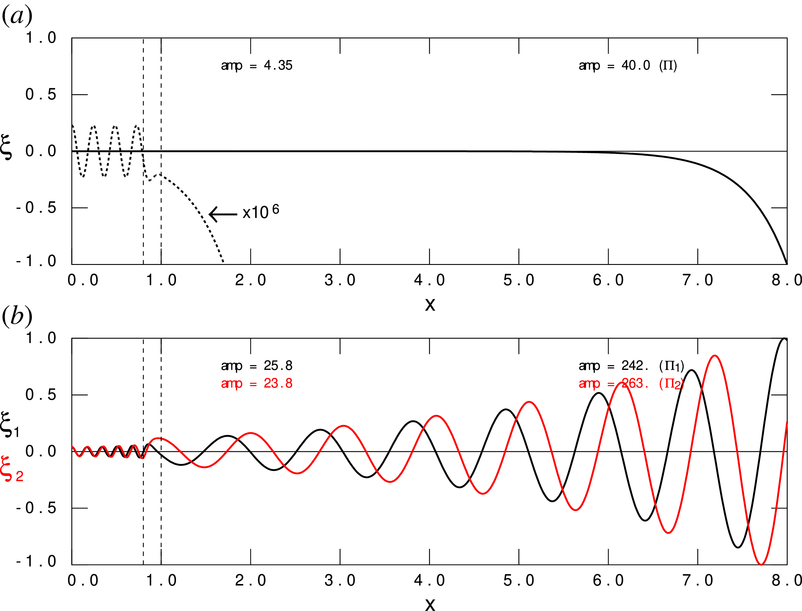
Figure 10 Long description
The image contains two graphs labeled (a) and (b), illustrating the eigenvalue spectra of electrodynamic waves in dielectric media. Graph (a) shows a real, unbound, discrete mode with specific parameters on the interval. Due to the huge exponential growth, the eigenfunction is magnified by a factor to highlight the oscillations in the internal part of the interval. Graph (b) displays a complex, leaky, discrete mode with different parameters on the same interval. Both graphs use the same parameters as in a previous figure, indicating a comparison or continuation of analysis. The real mode in graph (a) is represented by a black line, while the complex mode in graph (b) is shown with both black and red lines, indicating different components of the mode. The x-axis represents the spatial coordinate, and the y-axis represents the eigenfunction values. The graphs demonstrate the behavior of these modes within the specified interval, with annotations indicating the amplitude of the oscillations.
The first proviso concerns the methodology of coronal seismology. As mentioned previously, its task is to solve the inverse spectral problem, i.e. the iterative determination of the possible distributions of the equilibrium fields of a certain loop that has produced an observed spectrum. This is a gigantic task, not even approximately started, witnessed by the many sharp-boundary model calculations still in use in this field. Nevertheless, in principle, it can be carried out. The second proviso is a more serious one because it concerns the fundamentals of spectral theory. The initial perturbations that should be permitted in the solution of the inverse spectral problem are discussed in § 4.1. This analysis gives the transparent solution (4.15): the response to an arbitrary initial perturbation $X(x;\omega _n)$
is given by the sum over all discrete exponentials multiplied by an integral over all space involving the initial perturbation. Here, the central problem of leaky modes is manifest. One should admit arbitrary initial data for an honest comparison of the responses in different configurations, but the integrals clearly diverge for leaky modes. This brings us back to the problem of normalisation discussed in § 4.2. As discussed there, the oscillatory solutions for the leaky EM waves shown in figure 6, corresponding to the spectrum shown in figure 4, precisely cancel out the contributions of the two fields in the external region to produce satisfaction of the normalisation (4.29) of the quasi-normal modes: systematic cutoff guaranteed! However, the oscillatory solutions for the leaky MHD waves shown in figure 10, corresponding to the spectrum shown in figure 8, do not cancel anything: there is no alternative for the regular normalisation. In that case, the initial impulse should be cutoff beyond a certain radius to prevent the exponentially increasing part of the solution to completely dominate the solution. The problem is: what cutoff radius to take? Its value will determine which part of the leaky mode spectrum will participate in the truncated problem and it will be different for the various equilibria and associated MHD spectra investigated. Consequently, cutoff criteria are completely arbitrary so that there is no guiding principle to interpret initial transients and a systematic use of leaky modes for coronal seismology is illusory.
$X(x;\omega _n)$
is given by the sum over all discrete exponentials multiplied by an integral over all space involving the initial perturbation. Here, the central problem of leaky modes is manifest. One should admit arbitrary initial data for an honest comparison of the responses in different configurations, but the integrals clearly diverge for leaky modes. This brings us back to the problem of normalisation discussed in § 4.2. As discussed there, the oscillatory solutions for the leaky EM waves shown in figure 6, corresponding to the spectrum shown in figure 4, precisely cancel out the contributions of the two fields in the external region to produce satisfaction of the normalisation (4.29) of the quasi-normal modes: systematic cutoff guaranteed! However, the oscillatory solutions for the leaky MHD waves shown in figure 10, corresponding to the spectrum shown in figure 8, do not cancel anything: there is no alternative for the regular normalisation. In that case, the initial impulse should be cutoff beyond a certain radius to prevent the exponentially increasing part of the solution to completely dominate the solution. The problem is: what cutoff radius to take? Its value will determine which part of the leaky mode spectrum will participate in the truncated problem and it will be different for the various equilibria and associated MHD spectra investigated. Consequently, cutoff criteria are completely arbitrary so that there is no guiding principle to interpret initial transients and a systematic use of leaky modes for coronal seismology is illusory.
In summary, for all the reasons given here, we maintain the final conclusion of our previous paper (Goedbloed et al. Reference Goedbloed, Keppens and Poedts2023): Exit leaky modes in coronal magnetic flux tubes!To which we now add: In particular, in solar seismology.
Acknowledgements
DIFFER is part of the institutes organisation of NWO.
Editor Thierry Passot thanks the referees for their advice in evaluating this article.
Funding
This research was supported by the KU Leuven (GOA/2015-014).
Declaration of interests
The authors report no conflict of interest.

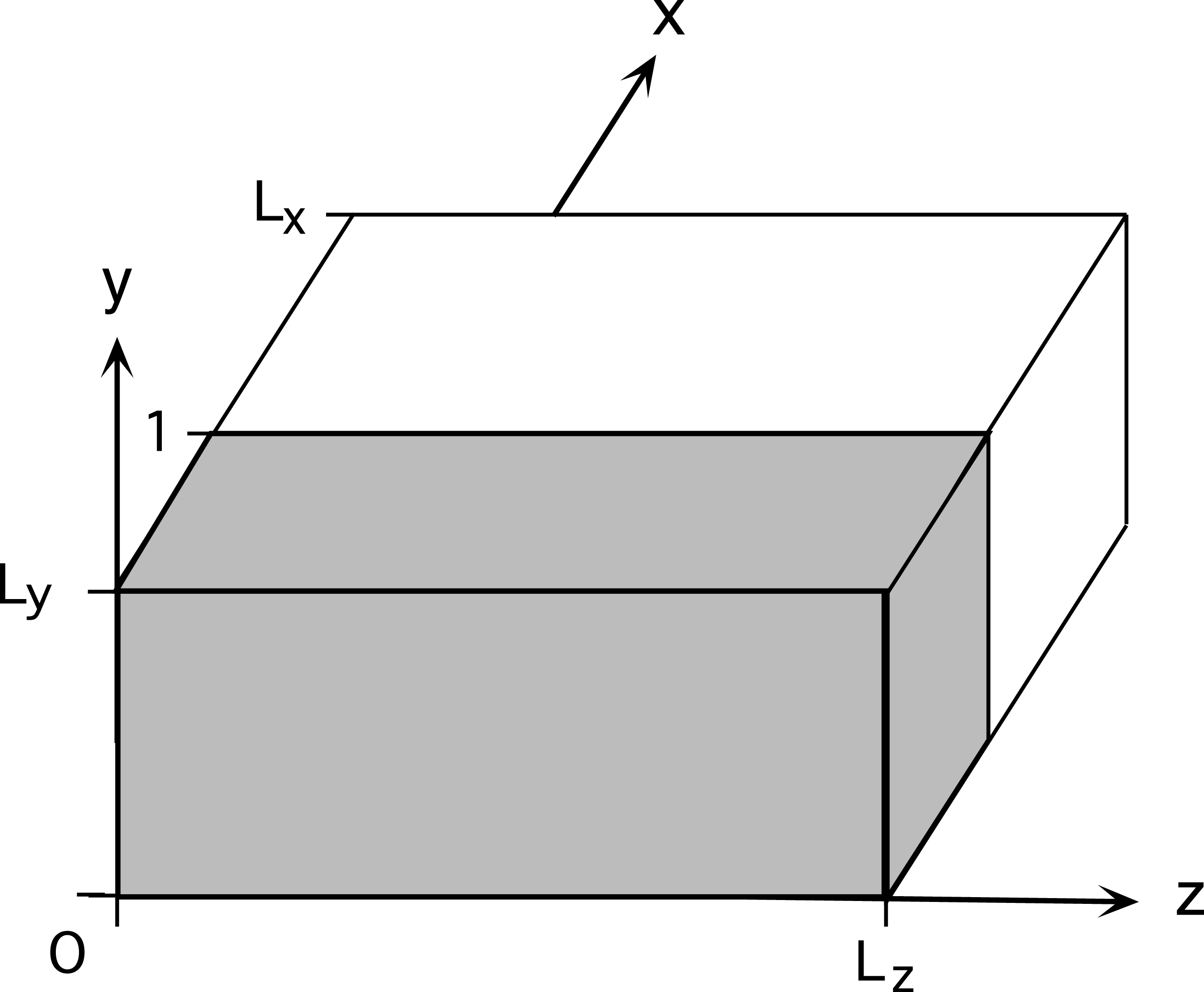
 Lx,Ly,Lz→∞
 v(x)
v(x) |x|⩽1
|x|⩽1 |x|=1
|x|=1 x
x x=0
x=0 a
a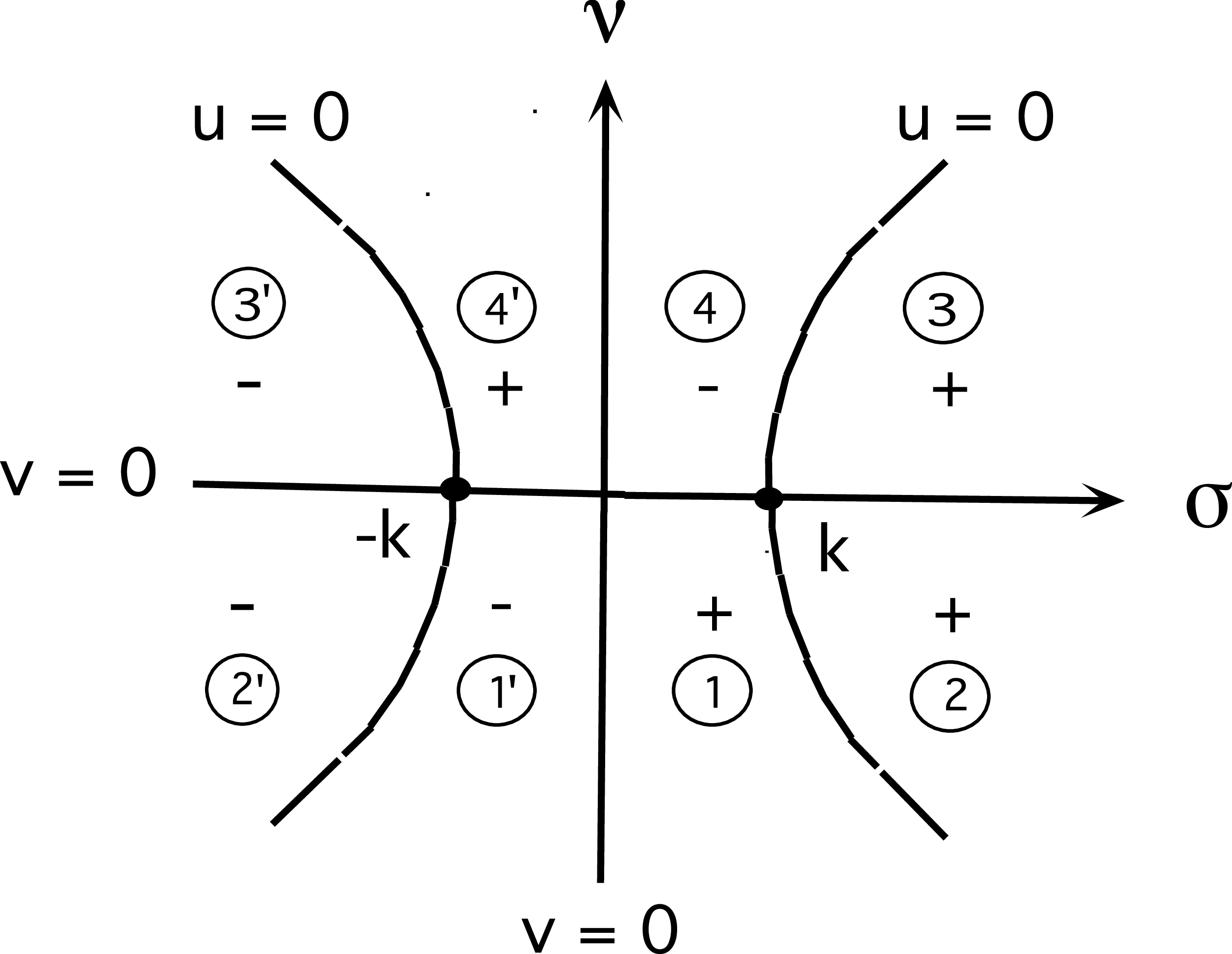
 ω
ω u=0
u=0 σ2−ν2=k2
 v=0
v=0 σ=0
σ=0 ν=0
ν=0 ±
± q^
q^ ①,u⩽0,ν⩽0
 −12π⩽φ<−14π⇒q^1⩾0,q^2<0
 ②,u>0,ν⩽0
 −14π<φ⩽0⇒q^1>0,q^2⩽0
 ③,u>0,ν>0
 0<φ<14π⇒q^1>0,q^2>0
 ④,u⩽0,ν>0
 14π⩽φ<12π⇒q^1<0,q^2<0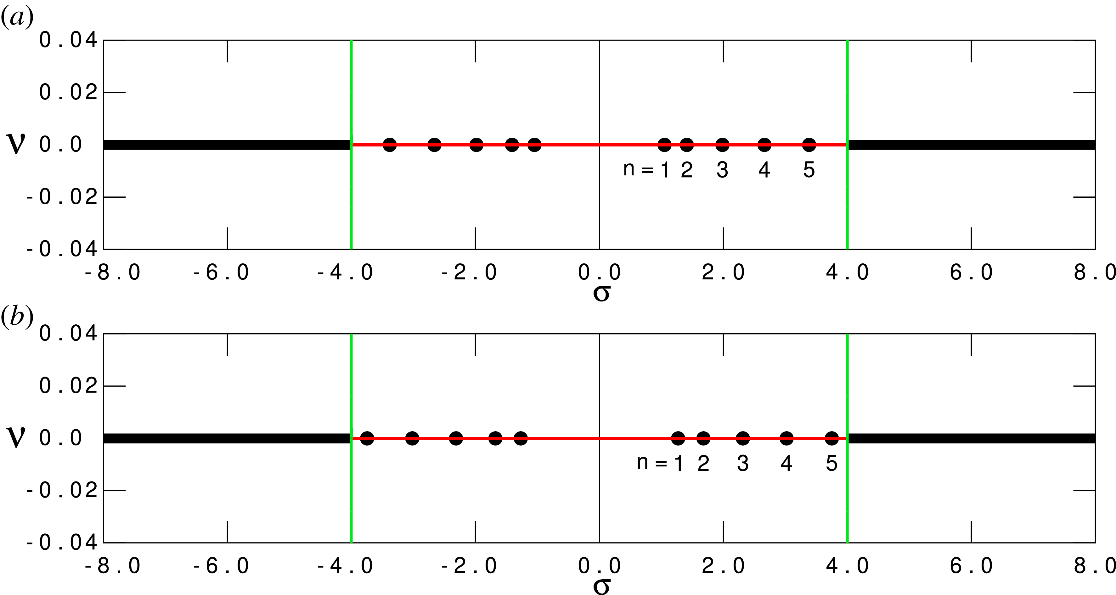
 v(x)
v(x) δ=0.25
 ϵ=0.02
 |x|=1
|x|=1 z
z k=4.0
k=4.0 n=1,…,5
 |σ|⩾k
|σ|⩾k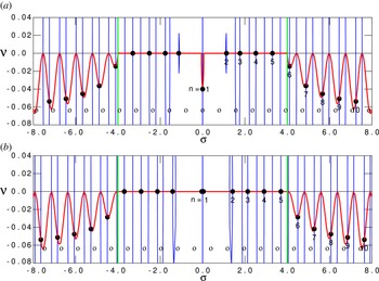
 δ
δ ϵ
ϵ k
k n=1,…,5
 |σ|⩾k
|σ|⩾k n=6,…,∞
 Scom=0
 E(1)=0
 k=0
k=0 ν=(1/2)δln[(1−δ)/(1+δ)]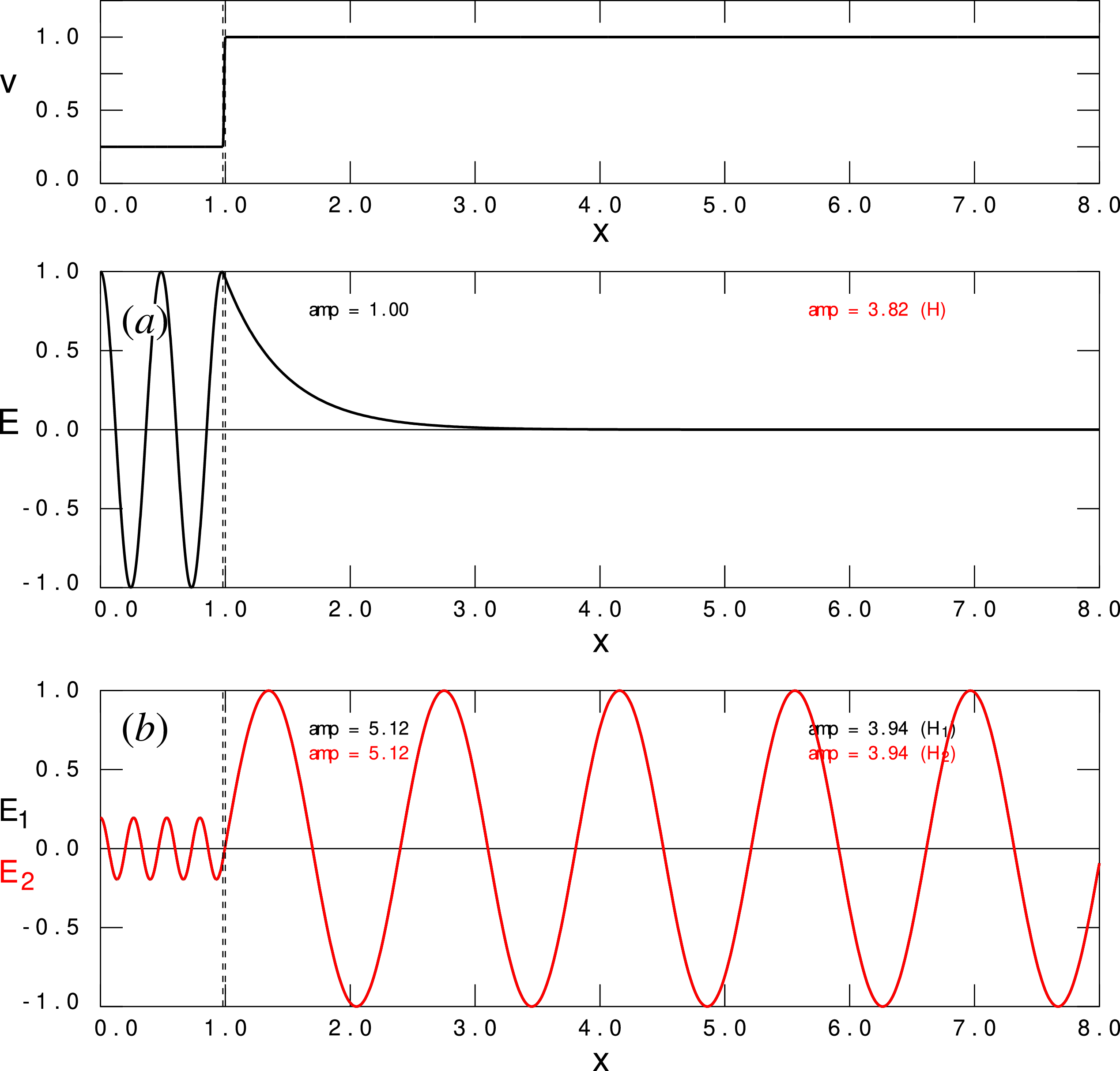
 n=5
n=5 σ=3.3813
 (0,8.0)
 σ=6.0
σ=6.0 v(x)
v(x) δ
δ ϵ
ϵ k
k H1,2(x)
 E1,2(x)
 |x|=1
|x|=1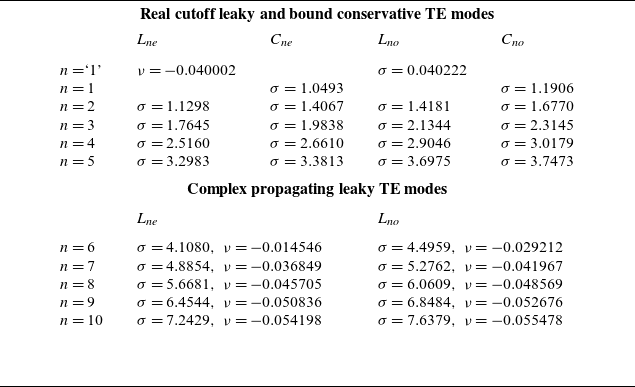
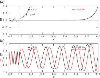
 n=4
n=4 σ=3.2983
 (0,8.0)
 106
106 n=9
n=9 σ=6.4545
 ν=−0.050836
 δ
δ ϵ
ϵ k
k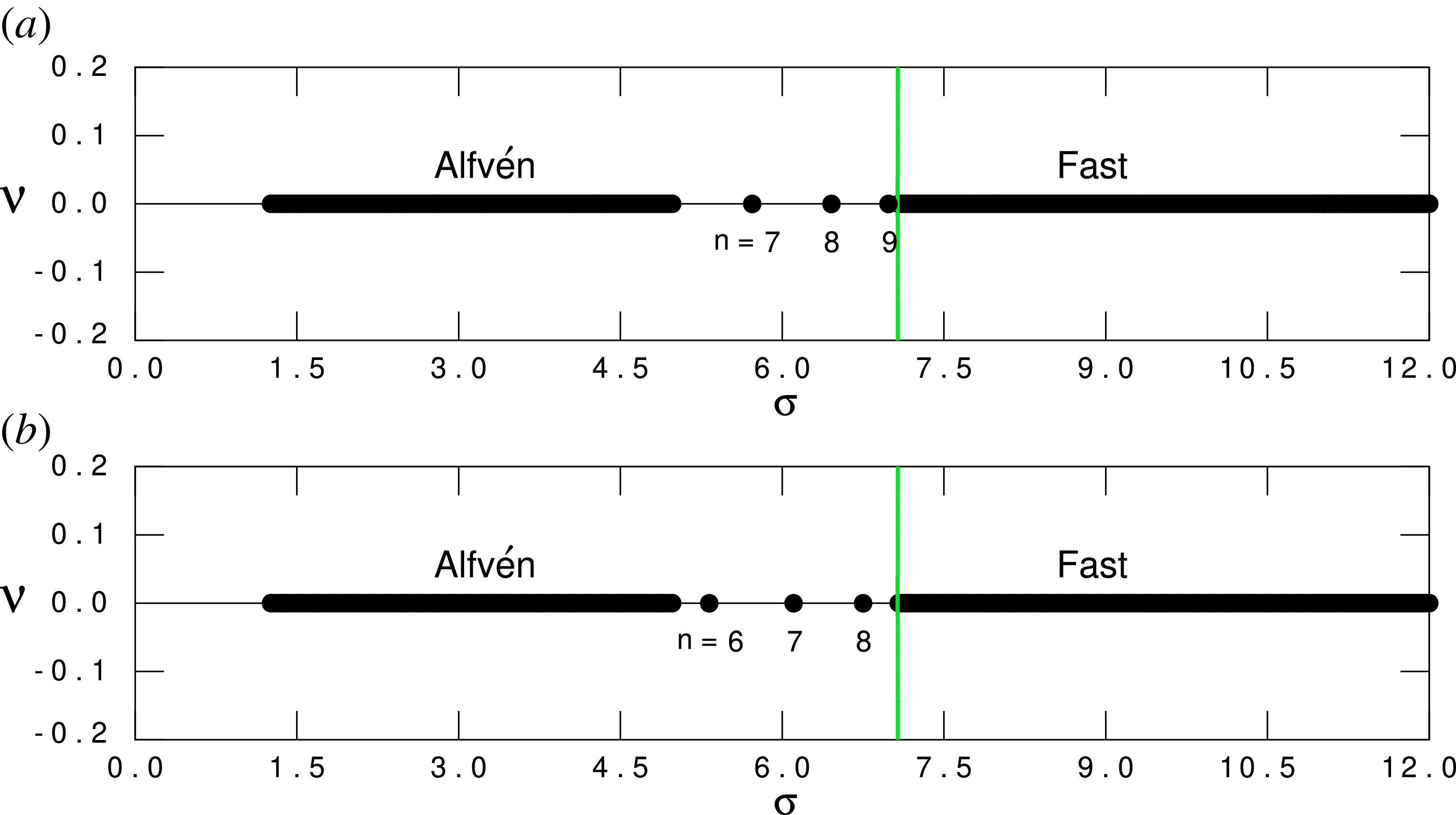
 ϵ=0.2
ϵ=0.2 δ=0.25
 k=ℓ=5.0
 n=1⋅s6
 n=1,…,5
 n=7,8,9
 n=6,7,8
 |σ|⩾ktot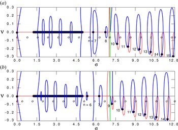
 n=7,8
n=7,8 n=6,7
n=6,7 |σ|⩾ktot
 |x|→∞
|x|→∞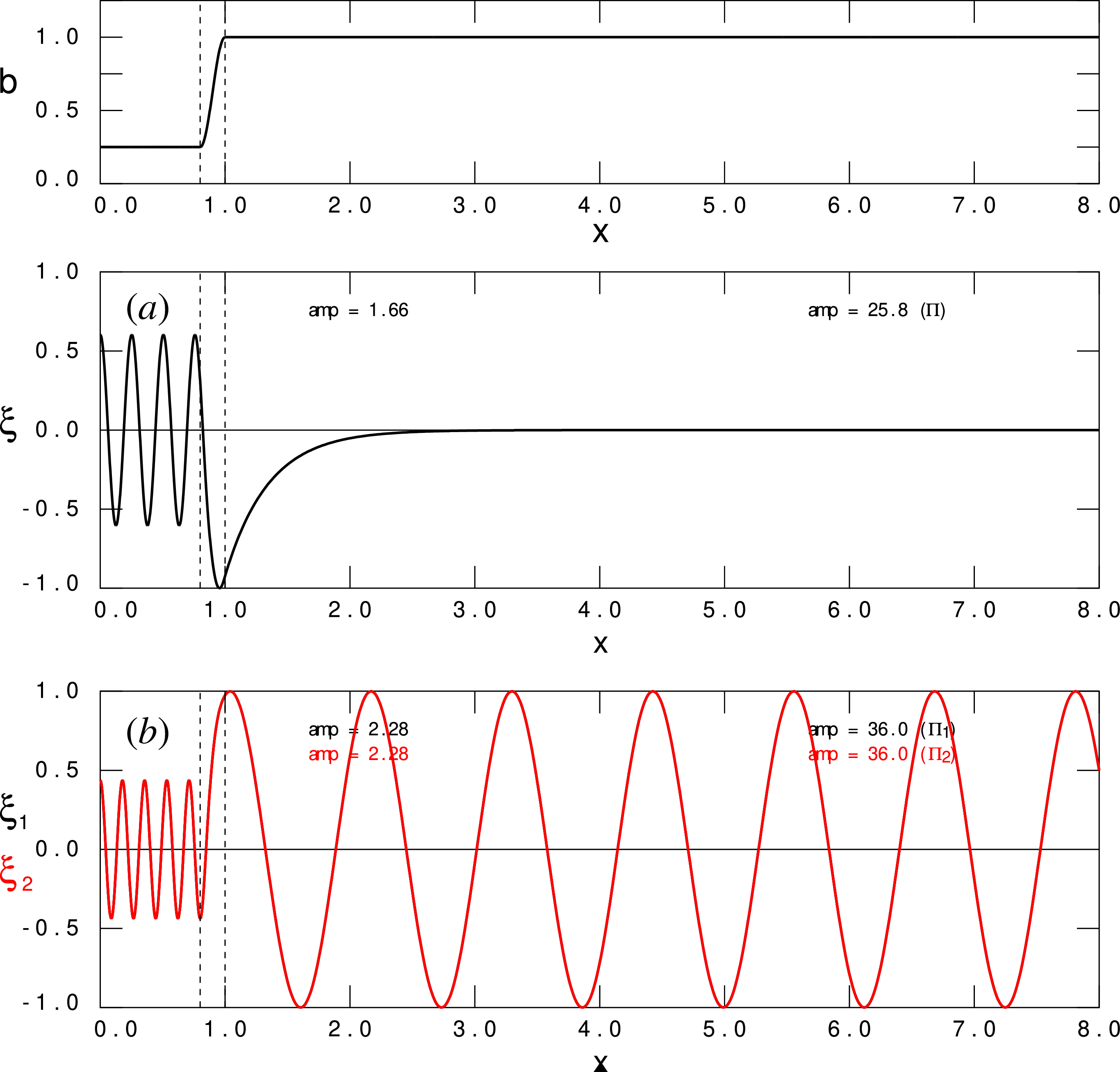
 n=8
n=8 σ=6.4563
 (0,8.0)
 σ=9.0
σ=9.0 b(x)
b(x) δ
δ ϵ
ϵ k
k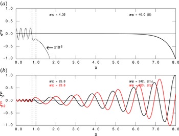
 n=8
n=8 σ=6.7219
 (0,8.0)
 106
106 n=12
n=12 σ=9.3059
 ν=−0.20632
 δ
δ ϵ
ϵ k
k
 Open access

