1. Introduction
The importance of drag reduction becomes essential in reducing both energy consumption and pollutant emissions in modern transportation systems. The transportation sector, which accounts for $25\,\%$
of the energy budget, is responsible for more than
$25\,\%$
of the energy budget, is responsible for more than $10\,\%$
of global greenhouse gases, as mentioned in Cheng et al. (Reference Cheng, Qiao, Zhang, Quadrio and Zhou2021). Skin friction is a crucial contributor to drag, accounting for more than
$10\,\%$
of global greenhouse gases, as mentioned in Cheng et al. (Reference Cheng, Qiao, Zhang, Quadrio and Zhou2021). Skin friction is a crucial contributor to drag, accounting for more than $50\,\%$
of the total drag for commercial aircraft.
$50\,\%$
of the total drag for commercial aircraft.
Active control techniques have shown promise in reducing skin friction, with studies such as Choi, Moin & Kim (Reference Choi, Moin and Kim1994) demonstrating the effectiveness of specific approaches. Their direct numerical simulations (DNS) revealed that by applying blowing and suction at the wall, with velocities equal in magnitude but opposite in direction to those at a specified wall-normal location (known as the detection plane), skin-friction reduction up to $25\,\%$
can be obtained. Opposition control achieves drag reduction by forming a ‘virtual wall’, an effective plane with no through-flow, located half-way between the detection point and the wall. This virtual wall blocks the downwash of high-speed fluid during sweep events, preventing it from reaching the wall. Furthermore, they observed that drag reduction was most effective when the detection plane was positioned close to the wall at
$25\,\%$
can be obtained. Opposition control achieves drag reduction by forming a ‘virtual wall’, an effective plane with no through-flow, located half-way between the detection point and the wall. This virtual wall blocks the downwash of high-speed fluid during sweep events, preventing it from reaching the wall. Furthermore, they observed that drag reduction was most effective when the detection plane was positioned close to the wall at $y_d^+ = y_d u_\tau /\nu = 10$
, where
$y_d^+ = y_d u_\tau /\nu = 10$
, where $y_d$
is the distance of the detection plane from the wall,
$y_d$
is the distance of the detection plane from the wall, $u_\tau$
is the friction velocity and
$u_\tau$
is the friction velocity and $\nu$
is the kinematic viscosity. The superscript
$\nu$
is the kinematic viscosity. The superscript $+$
denotes, here and in the following, quantities in wall units. Subsequently, Hammond, Bewley & Moin (Reference Hammond, Bewley and Moin1998) conducted an analysis to determine the optimal positioning of the detection plane, concluding that the optimal position was at
$+$
denotes, here and in the following, quantities in wall units. Subsequently, Hammond, Bewley & Moin (Reference Hammond, Bewley and Moin1998) conducted an analysis to determine the optimal positioning of the detection plane, concluding that the optimal position was at $y^+=15$
. Positioning the detection plane closer or farther from the wall led to a significant increase in drag. Later, Chung & Sung (Reference Chung and Sung2003) found that drag reduction due to opposition control is not strongly affected by the position of the detection plane if it is placed between
$y^+=15$
. Positioning the detection plane closer or farther from the wall led to a significant increase in drag. Later, Chung & Sung (Reference Chung and Sung2003) found that drag reduction due to opposition control is not strongly affected by the position of the detection plane if it is placed between $10\lt y_d^+\lt 20$
. Chung & Talha (Reference Chung and Talha2011) demonstrated that the effectiveness of active control for skin-friction drag reduction is highly dependent on the amplitude of wall blowing and suction, as well as the detection plane location. The study found that drag reduction increases proportionally to the wall blowing and suction strength up to a critical threshold, beyond which the method becomes less effective.
$10\lt y_d^+\lt 20$
. Chung & Talha (Reference Chung and Talha2011) demonstrated that the effectiveness of active control for skin-friction drag reduction is highly dependent on the amplitude of wall blowing and suction, as well as the detection plane location. The study found that drag reduction increases proportionally to the wall blowing and suction strength up to a critical threshold, beyond which the method becomes less effective.
Kang & Choi (Reference Kang and Choi2000) through a numerical analysis were able to achieve up to $17\,\%$
of drag reduction by dynamically deforming the local wall surface in a turbulent channel flow. In their study, the wall surface was moved up and down, counteracting the wall-normal velocity detected at
$17\,\%$
of drag reduction by dynamically deforming the local wall surface in a turbulent channel flow. In their study, the wall surface was moved up and down, counteracting the wall-normal velocity detected at $y_d^+=10$
. However, it is worth noting that the amount of drag reduction achieved with this technique was lower than that observed by Choi et al. (Reference Choi, Moin and Kim1994) using active blowing and suction. Chang, Collis & Ramakrishnan (Reference Chang, Collis and Ramakrishnan2002) applied the opposition control strategy in a large eddy simulation of a turbulent channel flow. They found that as the friction Reynolds number
$y_d^+=10$
. However, it is worth noting that the amount of drag reduction achieved with this technique was lower than that observed by Choi et al. (Reference Choi, Moin and Kim1994) using active blowing and suction. Chang, Collis & Ramakrishnan (Reference Chang, Collis and Ramakrishnan2002) applied the opposition control strategy in a large eddy simulation of a turbulent channel flow. They found that as the friction Reynolds number $\textit{Re}_\tau = u_\tau h / \nu$
, where
$\textit{Re}_\tau = u_\tau h / \nu$
, where $h$
is the channel half-height, increased from
$h$
is the channel half-height, increased from $100$
to
$100$
to $720$
, the drag reduction decreased from
$720$
, the drag reduction decreased from $26\,\%$
to
$26\,\%$
to $19\,\%$
, indicating a decline in the efficiency of opposition control at higher Reynolds numbers. Similarly, opposition control applied by Yao, García & Hussain (Reference Yao, García and Hussain2025) to a DNS of a turbulent channel flow reported a drag reduction of approximately
$19\,\%$
, indicating a decline in the efficiency of opposition control at higher Reynolds numbers. Similarly, opposition control applied by Yao, García & Hussain (Reference Yao, García and Hussain2025) to a DNS of a turbulent channel flow reported a drag reduction of approximately $22.3\,\%$
at
$22.3\,\%$
at $\textit{Re}_\tau = 200$
, which decreased to about
$\textit{Re}_\tau = 200$
, which decreased to about $18.1\,\%$
at
$18.1\,\%$
at $\textit{Re}_\tau = 2000$
. Moreover, the distance of the detection plane from the wall
$\textit{Re}_\tau = 2000$
. Moreover, the distance of the detection plane from the wall $y_d^+$
was found to shift slightly inward with increasing
$y_d^+$
was found to shift slightly inward with increasing $\textit{Re}_\tau$
. Han & Huang (Reference Han and Huang2020) and Park & Choi (Reference Park and Choi2020) applied convolutional neural networks to predict wall-normal velocity fluctuations at the detection plane to replicate the effects of opposition control based only on wall measurements.
$\textit{Re}_\tau$
. Han & Huang (Reference Han and Huang2020) and Park & Choi (Reference Park and Choi2020) applied convolutional neural networks to predict wall-normal velocity fluctuations at the detection plane to replicate the effects of opposition control based only on wall measurements.
Direct numerical simulation studies of turbulent wall flow demonstrated that opposition control effectively reduces turbulent skin-friction drag. However, these simulations required complete velocity information at the detection plane, with drag reduction proportional to the amount of data available. Additionally, the control was applied instantly, which is not feasible in physical experiments such as wind tunnel tests, raising concerns about the practicality of implementing opposition control in real-world applications. A successful physical experiment, albeit via an offline control, of the opposition control strategy applied to near-wall turbulence was the one conducted by Rebbeck & Choi (Reference Rebbeck and Choi2001). By using a single detector and actuator in a wind tunnel they selectively cancelled the downwash of high-speed fluid during sweep events, showing the capabilities of this type of control in reducing skin friction. Their approach involved operating a piston-type actuator at fixed cycles to produce wall-normal jets, while continuously sampling velocity signals from hot-wire sensors. By conditionally sampling and ensemble averaging only the instances where the actuator correctly targeted sweep events they showed significant reductions in sweep intensity up to a streamwise distance $x^+ = 90$
downstream of the actuator. Later, a real-time experiment was implemented by Rebbeck & Choi (Reference Rebbeck and Choi2006). They conducted a wind tunnel experiment to investigate real-time opposition control analysing how the near-wall turbulence structure of the boundary layer is modified when opposition control is applied to individual sweep events through the use of a wall-normal jet. Their findings indicated that the wall-ward movement of high-speed fluid during sweep events can be effectively countered by a wall-normal jet produced by a loudspeaker actuator. This implies that opposition control of wall turbulence has the potential to reduce the skin-friction drag in the turbulent boundary layer. In more recent years, the opposition control technique has been extended to target large-scale motions in turbulent flows, as demonstrated in Abbassi et al. (Reference Abbassi, Baars, Hutchins and Marusic2017) and Dacome et al. (Reference Dacome, Mörsch, Kotsonis and Baars2024). They were able to achieve a reduction in both streamwise energy and skin friction. Additionally, the opposition control strategy has been applied to turbulent spots, as explored in Wang et al. (Reference Wang, Choi, Gaster, Atkin, Borodulin and Kachanov2021, Reference Wang, Choi, Gaster, Atkin, Borodulin and Kachanov2022). The findings of these two studies demonstrate the effectiveness of opposition control in cancelling the high-speed regions within turbulent spots and reducing root-mean-square velocity fluctuations near the wall.
$x^+ = 90$
downstream of the actuator. Later, a real-time experiment was implemented by Rebbeck & Choi (Reference Rebbeck and Choi2006). They conducted a wind tunnel experiment to investigate real-time opposition control analysing how the near-wall turbulence structure of the boundary layer is modified when opposition control is applied to individual sweep events through the use of a wall-normal jet. Their findings indicated that the wall-ward movement of high-speed fluid during sweep events can be effectively countered by a wall-normal jet produced by a loudspeaker actuator. This implies that opposition control of wall turbulence has the potential to reduce the skin-friction drag in the turbulent boundary layer. In more recent years, the opposition control technique has been extended to target large-scale motions in turbulent flows, as demonstrated in Abbassi et al. (Reference Abbassi, Baars, Hutchins and Marusic2017) and Dacome et al. (Reference Dacome, Mörsch, Kotsonis and Baars2024). They were able to achieve a reduction in both streamwise energy and skin friction. Additionally, the opposition control strategy has been applied to turbulent spots, as explored in Wang et al. (Reference Wang, Choi, Gaster, Atkin, Borodulin and Kachanov2021, Reference Wang, Choi, Gaster, Atkin, Borodulin and Kachanov2022). The findings of these two studies demonstrate the effectiveness of opposition control in cancelling the high-speed regions within turbulent spots and reducing root-mean-square velocity fluctuations near the wall.
In the case of active control it is often essential to identify the optimal actuation parameters to maximise effectiveness. This can be achieved using optimisation techniques such as Bayesian optimisation (BO). Bayesian optimisation is one of the most popular ‘surrogate-based’, derivative-free, global optimisation tools, particularly effective for expensive, non-convex objective functions (Gelbart, Snoek & Adams Reference Gelbart, Snoek and Adams2014) and popularised by the efficient global optimisation algorithm introduced by Jones, Schonlau & Welch (Reference Jones, Schonlau and Welch1998). It is ideal for optimising continuous domains with fewer than 20 dimensions and can handle stochastic noise in function evaluations (Frazier Reference Frazier2018). It constructs a surrogate model for the objective function, quantifies uncertainty using Gaussian process regression (Rasmussen & Williams Reference Rasmussen and Williams2008) and employs an acquisition function derived from the surrogate to determine the next sampling point. Many reviews (Swersky, Snoek & Adams Reference Swersky, Snoek and Adams2013; Frazier Reference Frazier2018; Wang et al. Reference Wang, Jin, Schmitt and Olhofer2023) show different application areas of this algorithm including robotics (Lizotte et al. Reference Lizotte, Wang, Bowling and Schuurmans2007; Martinez-Cantin et al. Reference Martinez-Cantin, de Freitas, Doucet and Castellanos2007), automatic machine learning (Snoek, Larochelle & Adams Reference Snoek, Larochelle and Adams2012; Swersky et al. Reference Swersky, Snoek and Adams2013) and experimental design (Bardenet et al. Reference Bardenet, Brendel, Kégl and Sebag2013). Talnikar et al. (Reference Talnikar, Blonigan, Bodart and Wang2014) developed a parallel BO algorithm specifically for large eddy simulations, which are computationally expensive and involve noisy objective functions. Their approach was used to minimise drag in turbulent channel flows and to optimise the design of a turbine blade. Mahfoze et al. (Reference Mahfoze, Moody, Wynn, Whalley and Laizet2019) applied BO to determine the optimal amplitude and coverage parameters for wall-normal blowing control in a zero-pressure-gradient turbulent boundary layer, achieving significant skin-friction reductions. More recently, Blanchard et al. (Reference Blanchard, Cornejo Maceda, Fan, Li, Zhou, Noack and Sapsis2021) applied the BO algorithm to reduce the drag in the fluidic pinball and to enhance the mixing in a turbulent jet. Pino et al. (Reference Pino, Schena, Rabault and Mendez2023) conducted a comparative analysis of two global optimisation techniques, BO and Lipschitz global optimisation, against two machine learning methods, genetic programming and reinforcement learning. These control algorithms were tested on three different cases: stabilising a nonlinear dynamical system with frequency cross-talk, wave cancellation in a Burgers’ flow and drag reduction in a cylinder wake flow.
The present study investigates the possibility of optimising the actuation parameters through a BO algorithm in a real-time opposition control experiment, with the objective of reducing sweep event intensity in a fully turbulent channel flow. The results indicate that optimising the control parameters is achievable by employing an appropriate cost function. Moreover, the conditional analysis applied to the velocity signals showed an overall energy increase in the controlled case for the optimal set of control parameters identified through the BO algorithm and highlighted the large reduction of the sweep event convection velocity during the jet-blowing phase.
2. Experimental set-up
Experiments were conducted in an 8-metre-long duct with a $7 \times{30}\,\textrm {cm}^{2}$
rectangular cross-section leading to an aspect ratio of
$7 \times{30}\,\textrm {cm}^{2}$
rectangular cross-section leading to an aspect ratio of $4.28$
. A centreline velocity of
$4.28$
. A centreline velocity of $U_0 = {3.2}{\,\textrm {m s}}^{-1}$
was imposed. The friction velocity was
$U_0 = {3.2}{\,\textrm {m s}}^{-1}$
was imposed. The friction velocity was $u_\tau = {0.162}{\,\textrm {m s}}^{-1}$
, which leads to a friction Reynolds number of
$u_\tau = {0.162}{\,\textrm {m s}}^{-1}$
, which leads to a friction Reynolds number of $\textit{Re}_\tau \approx 350$
, a viscous length of
$\textit{Re}_\tau \approx 350$
, a viscous length of $l_\tau = \nu /u_\tau = {9.89\times {10}^{-05}}\,\textrm {m}$
and a viscous time of
$l_\tau = \nu /u_\tau = {9.89\times {10}^{-05}}\,\textrm {m}$
and a viscous time of $t_\tau = \nu /u_\tau ^2 = {6.1\times {10}^{-4}}\,\textrm {s}$
. The instantaneous velocity components
$t_\tau = \nu /u_\tau ^2 = {6.1\times {10}^{-4}}\,\textrm {s}$
. The instantaneous velocity components $(U, V, W)$
, respectively streamwise, wall-normal and spanwise components, can be decomposed in a mean contribution
$(U, V, W)$
, respectively streamwise, wall-normal and spanwise components, can be decomposed in a mean contribution $(\overline {U}, \overline {V}, \overline {W})$
and a fluctuating one
$(\overline {U}, \overline {V}, \overline {W})$
and a fluctuating one $(u, v, w)$
. Channel flow statistics profiles are presented in figure 1. Data from the present experiment are indicated with continuous lines and circle markers, while DNS data taken from Moser, Kim & Mansour (Reference Moser1999) at
$(u, v, w)$
. Channel flow statistics profiles are presented in figure 1. Data from the present experiment are indicated with continuous lines and circle markers, while DNS data taken from Moser, Kim & Mansour (Reference Moser1999) at $\textit{Re}_\tau =395$
are indicated with dashed lines. Figure 1(a,b,c,d) shows the mean velocity profile, the streamwise Reynolds stresses, skewness and flatness, respectively.
$\textit{Re}_\tau =395$
are indicated with dashed lines. Figure 1(a,b,c,d) shows the mean velocity profile, the streamwise Reynolds stresses, skewness and flatness, respectively.

Figure 1. Channel flow statistics. Continuous lines with circle markers indicate the canonical case, dashed lines indicate DNS data statistics taken from Moser et al. (Reference Moser1999). (a) Mean velocity $\overline {U}^+$
, (b) streamwise component of the Reynolds stresses
$\overline {U}^+$
, (b) streamwise component of the Reynolds stresses $\overline {uu}^+$
, (c) skewness
$\overline {uu}^+$
, (c) skewness $S(U)$
, (d) flatness
$S(U)$
, (d) flatness $F(U)$
.
$F(U)$
.
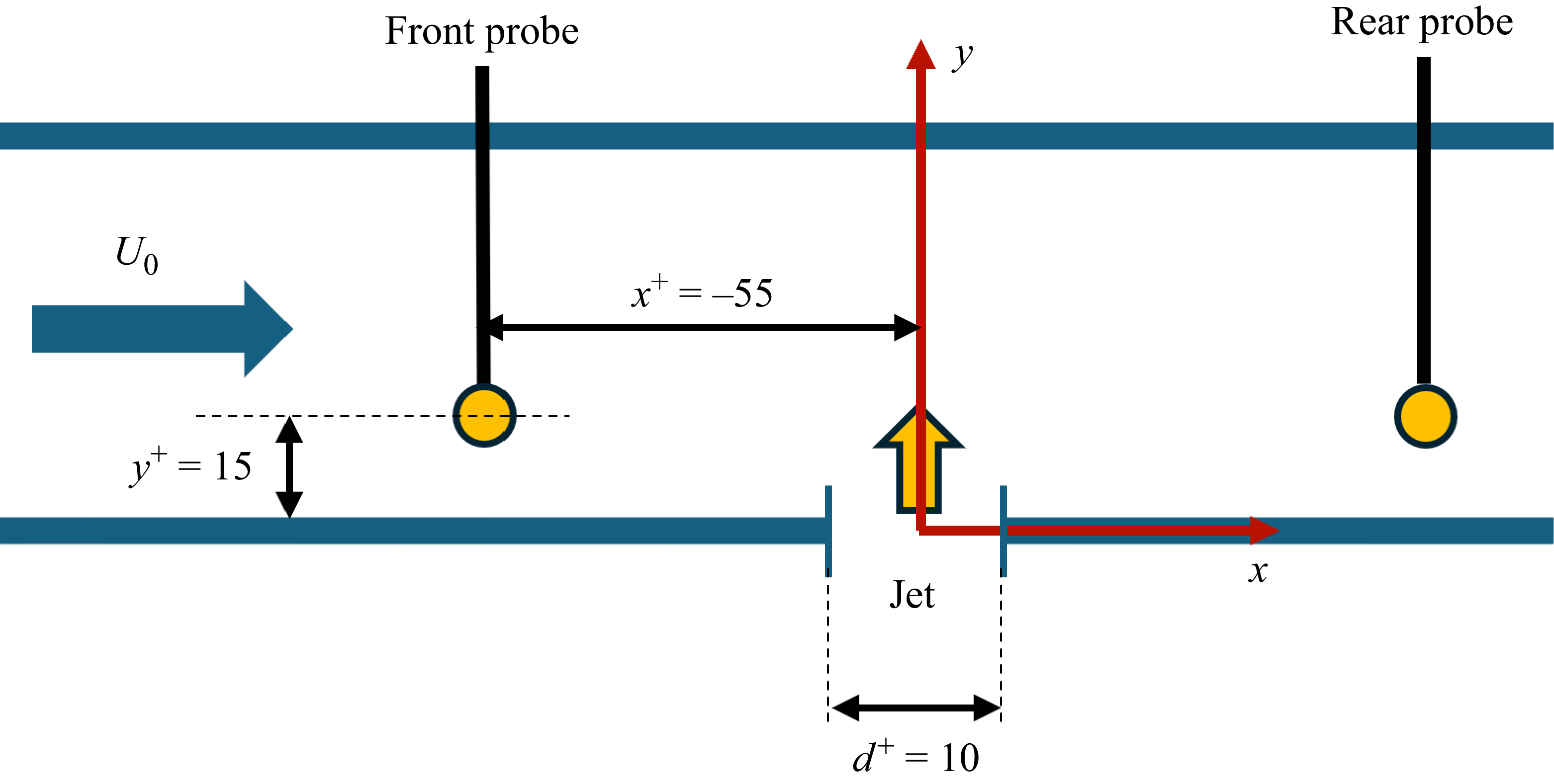
In the present experiment, two hot-wire probes were used, both connected to a Dantec 55M10 CTA standard bridge. The front probe, a Dantec 55P11, was positioned upstream of the jet orifice at $x^+ = -55$
and a wall-normal distance of
$x^+ = -55$
and a wall-normal distance of $y^+ = 15$
, with the centre of the jet orifice serving as the origin of the reference system. The streamwise position of the front probe was selected following the approach taken in the experiments carried out by Rebbeck & Choi (Reference Rebbeck and Choi2001, Reference Rebbeck and Choi2006) to account for both the convective time and the delay time associated with the control system. It can be noted that, in the current experiment, the actuation delay time can be modulated through a microcontroller. The rear probe, a Dantec 55P15 boundary layer probe, was mounted on a two-axis movable stand to allow movements in the streamwise and wall-normal directions. The positional accuracy of the streamwise axis, achieved using the OptoSigma OSMS33-500(X) stage, is
$y^+ = 15$
, with the centre of the jet orifice serving as the origin of the reference system. The streamwise position of the front probe was selected following the approach taken in the experiments carried out by Rebbeck & Choi (Reference Rebbeck and Choi2001, Reference Rebbeck and Choi2006) to account for both the convective time and the delay time associated with the control system. It can be noted that, in the current experiment, the actuation delay time can be modulated through a microcontroller. The rear probe, a Dantec 55P15 boundary layer probe, was mounted on a two-axis movable stand to allow movements in the streamwise and wall-normal directions. The positional accuracy of the streamwise axis, achieved using the OptoSigma OSMS33-500(X) stage, is ${25}\,\mu {\textrm {m}}$
while the wall-normal axis, guided by the OptoSigma OSMS26-300(Z) stage, is
${25}\,\mu {\textrm {m}}$
while the wall-normal axis, guided by the OptoSigma OSMS26-300(Z) stage, is ${40}\,\mu {\textrm {m}}$
. A schematic view of the probes’ positioning is shown in figure 2. Both hot-wire probes feature a sensitive tungsten wire measuring
${40}\,\mu {\textrm {m}}$
. A schematic view of the probes’ positioning is shown in figure 2. Both hot-wire probes feature a sensitive tungsten wire measuring ${5}\,\mu {\textrm {m}}$
in diameter and
${5}\,\mu {\textrm {m}}$
in diameter and ${1.25}\,\textrm {mm}$
in length and were calibrated in situ. Hot-wire calibration curves were fitted using the King’s law and signals were collected by a National Instruments PCI-MIO-16-XE-10 16-bit DAQ board at a sample rate of
${1.25}\,\textrm {mm}$
in length and were calibrated in situ. Hot-wire calibration curves were fitted using the King’s law and signals were collected by a National Instruments PCI-MIO-16-XE-10 16-bit DAQ board at a sample rate of ${10}\,\textrm {KHz}$ $ ( f^+_{{HW}} = 6.1 )$
.
$ ( f^+_{{HW}} = 6.1 )$
.

Figure 2. Sketch of the real-time opposition control experimental set-up. The airflow proceeds from left to right. The front probe is positioned at $x^+ = -55$
and
$x^+ = -55$
and $y^+ =15$
. The position of the rear probe can be adjusted in both
$y^+ =15$
. The position of the rear probe can be adjusted in both $x$
and
$x$
and $y$
directions.
$y$
directions.
The National Instrument acquisition board was connected to the PCI bus of a laboratory workstation. Data post-processing and the BO algorithm were executed on a laptop connected to the workstation via LAN. A server-based Python algorithm leveraging Python’s built-in socket library was loaded onto the workstation, while a client-based script was executed on the laptop. Typically, the client (laptop) initiates a query to the server (workstation), which may involve executing a measurement or modifying a control policy. Once the server processes the request, the client retrieves feedback or a data buffer if a signal has been acquired. The laptop then processes the raw signal data.
3. Detection technique and control hardware
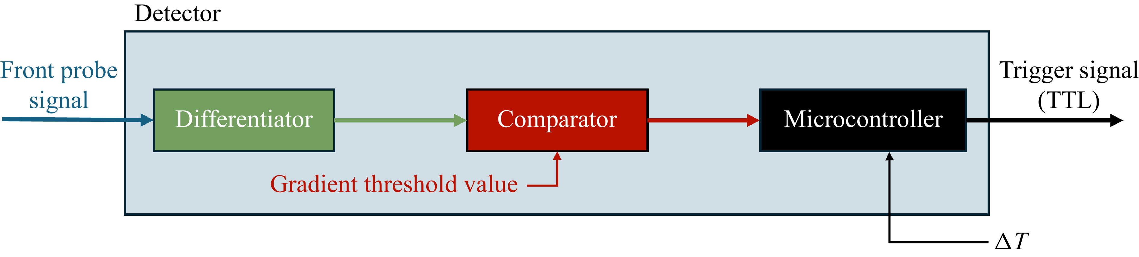
Following the work of Rebbeck & Choi (Reference Rebbeck and Choi2006), sweep events were detected using the velocity gradient technique applied to the longitudinal component of the velocity, measured by the front probe. The detection scheme is illustrated in figure 3. The signal obtained from the front probe is differentiated through an analogue differentiator to compute its time derivative. Subsequently, a comparator device identifies sweep events and generates a transistor–transistor logic (TTL) signal whenever the time derivative exceeds a predefined threshold. This signal is subsequently delayed via a microcontroller to account for the convection time and the control actuator response time. In figure 4 the velocity signal sampled by the front probe is represented as a continuous blue line, while its time derivative is depicted as a continuous green line. The dashed red vertical lines indicate the instants at which events are detected. This technique allowed the sweep event detection to be carried out in real time. The comparator threshold level has been set to ensure that both the gradient technique and the variable-interval time-averaging (VITA) technique (Blackwelder & Kaplan Reference Blackwelder and Kaplan1976) detected a comparable number of events. For a fluctuating quantity $Q(x_i, t)$
, the variable-interval time average is defined as
$Q(x_i, t)$
, the variable-interval time average is defined as
 \begin{equation} \widehat {Q}(x_i, t, T) = \frac {1}{T} \int _{t-\frac {1}{2}T}^{{t+\frac {1}{2}T}} Q(x_i, s)\, {\rm d}s , \end{equation}
where $T$
is the averaging time. Sweep events detection, in the VITA technique, is defined as
$T$
is the averaging time. Sweep events detection, in the VITA technique, is defined as
 \begin{equation} D(t) = \begin{cases} 1, & \text{if } \quad \widehat {v\textit{ar}} \gt \textit{k u}_{\textit{rms}}^2\\ 0, & \text{otherwise} \end{cases}, \end{equation}
where the localised variance of streamwise velocity fluctuation $u$
is
$u$
is
 \begin{equation} \widehat {v\textit{ar}}(x_i, t, T) = \widehat {u^2}(x_i, t, T) - \left [ \widehat {u}(x_i, t, T) \right ]^2\!, \end{equation} $k$
is the threshold level and
$k$
is the threshold level and $u_{\textit{rms}}$
is the root mean square of the fluctuating velocity for the whole recorded signal. The comparator threshold for the gradient technique was set to have a similar number of VITA events with
$u_{\textit{rms}}$
is the root mean square of the fluctuating velocity for the whole recorded signal. The comparator threshold for the gradient technique was set to have a similar number of VITA events with $k = 1.0$
and
$k = 1.0$
and $T^+ = 10$
. These values match those reported in Rebbeck & Choi (Reference Rebbeck and Choi2006). A burst frequency of the sweep events detected using the tuned gradient technique was found to be
$T^+ = 10$
. These values match those reported in Rebbeck & Choi (Reference Rebbeck and Choi2006). A burst frequency of the sweep events detected using the tuned gradient technique was found to be $f^+_{\textit{sweep}} = {3.05\times {10}^{-3}}$
.
$f^+_{\textit{sweep}} = {3.05\times {10}^{-3}}$
.

Figure 3. Sweep event detector system scheme. Inputs are the front probe signal and the delay time, $\Delta T$
, applied to the TTL signal. The comparator threshold is kept constant. The output is the delayed TTL signal.
$\Delta T$
, applied to the TTL signal. The comparator threshold is kept constant. The output is the delayed TTL signal.

Figure 4. Visualisation of the sweep events detection technique. The continuous blue line is the longitudinal component of the front probe instantaneous velocity signal, $U$
, while the continuous green line represents its time derivative,
$U$
, while the continuous green line represents its time derivative, $\dot {U}$
. Red dashed vertical lines show the trigger instant. The starting time is arbitrary.
$\dot {U}$
. Red dashed vertical lines show the trigger instant. The starting time is arbitrary.
It can be observed in figure 2 that the front probe represented in the sketch was left intentionally fully exposed to the flow to have maximum flexibility in its placement. This set-up produces some flow perturbations that should be taken into account. However, it can be noted that the probe intrusiveness is not such as to highly affect the flow structure in the inner region compared with the canonical case. To evaluate the intrusiveness of the front probe, in figure 5 is illustrated the normalised burst frequency of sweep events, $n^+$
, as a function of
$n^+$
, as a function of $T^+$
for a given VITA threshold level
$T^+$
for a given VITA threshold level $k=1.0$
, measured using the rear probe positioned at
$k=1.0$
, measured using the rear probe positioned at $x^+=66$
and
$x^+=66$
and $y^+=15$
. The figure compares results for the canonical case (without the presence of the front probe) and the baseline case (with the front probe positioned at
$y^+=15$
. The figure compares results for the canonical case (without the presence of the front probe) and the baseline case (with the front probe positioned at $x^+=-55$
and
$x^+=-55$
and $y^+=15$
and the control actuator deactivated). A reasonable agreement between the canonical and the baseline case can be observed, representing that the number of events is not strongly affected by the presence of the front probe. Both results also agree with the DNS channel flow simulations carried out by Johansson, Alfredsson & Kim (Reference Johansson, Alfredsson and Kim1991) at
$y^+=15$
and the control actuator deactivated). A reasonable agreement between the canonical and the baseline case can be observed, representing that the number of events is not strongly affected by the presence of the front probe. Both results also agree with the DNS channel flow simulations carried out by Johansson, Alfredsson & Kim (Reference Johansson, Alfredsson and Kim1991) at $\textit{Re}_\tau =180$
. Figure 6(a) presents a comparison of the VITA conditionally averaged sweep events for the canonical and baseline flows. This analysis was applied to the velocity signal sampled by the rear probe positioned at
$\textit{Re}_\tau =180$
. Figure 6(a) presents a comparison of the VITA conditionally averaged sweep events for the canonical and baseline flows. This analysis was applied to the velocity signal sampled by the rear probe positioned at $x^+ =66$
and
$x^+ =66$
and $y^+=15$
using a threshold level
$y^+=15$
using a threshold level $k=1.0$
and an averaging time
$k=1.0$
and an averaging time $T^+=10$
. Canonical and baseline cases are respectively represented by continuous and dashed lines. The discrepancy between the canonical and baseline curves primarily arises from the slightly lower value of
$T^+=10$
. Canonical and baseline cases are respectively represented by continuous and dashed lines. The discrepancy between the canonical and baseline curves primarily arises from the slightly lower value of $u_{\textit{rms}}$
observed in the baseline case, where the rear probe is located in the wake of the upstream sensor. This reduction in
$u_{\textit{rms}}$
observed in the baseline case, where the rear probe is located in the wake of the upstream sensor. This reduction in $u_{\textit{rms}}$
is attributed to the intrusive effect of the upstream probe. Since the VITA detection threshold is defined as
$u_{\textit{rms}}$
is attributed to the intrusive effect of the upstream probe. Since the VITA detection threshold is defined as $k u_{\textit{rms}}$
, a lower
$k u_{\textit{rms}}$
, a lower $u_{\textit{rms}}$
results in a reduced threshold, leading to the identification of a greater number of events in the baseline case. This fact can explain why the burst frequency is slightly different between the canonical and the baseline curves of figure 5 and why the baseline VITA event shown in figure 6(a) presents a reduced amplitude around
$u_{\textit{rms}}$
results in a reduced threshold, leading to the identification of a greater number of events in the baseline case. This fact can explain why the burst frequency is slightly different between the canonical and the baseline curves of figure 5 and why the baseline VITA event shown in figure 6(a) presents a reduced amplitude around $t^+ = 10$
with respect to the canonical one. Differences up to
$t^+ = 10$
with respect to the canonical one. Differences up to $18\,\%$
between the canonical and the baseline case can be observed primarily in the positive and negative peaks of the VITA event shown in figure 6(a). Although this bias is non-negligible, it cannot be entirely removed given the current experimental set-up. It should be noted that this systematic bias affects both the baseline and controlled signals, as they are sampled under the same experimental configuration. Consequently, it does not compromise the direct comparison between the baseline and the controlled case. Figure 6(b) shows a comparison between the conditionally averaged sweep events detected using the VITA technique and the gradient technique, both sampled at
$18\,\%$
between the canonical and the baseline case can be observed primarily in the positive and negative peaks of the VITA event shown in figure 6(a). Although this bias is non-negligible, it cannot be entirely removed given the current experimental set-up. It should be noted that this systematic bias affects both the baseline and controlled signals, as they are sampled under the same experimental configuration. Consequently, it does not compromise the direct comparison between the baseline and the controlled case. Figure 6(b) shows a comparison between the conditionally averaged sweep events detected using the VITA technique and the gradient technique, both sampled at $x^+=66$
from the rear probe velocity signal in the canonical case. In the VITA method, the trigger for conditional averaging, unlike in figure 6(a) where it was computed from the rear probe positioned at
$x^+=66$
from the rear probe velocity signal in the canonical case. In the VITA method, the trigger for conditional averaging, unlike in figure 6(a) where it was computed from the rear probe positioned at $x^+=66$
, is here obtained from the front probe located at
$x^+=66$
, is here obtained from the front probe located at $x^+ = -55$
. Similarly, in the gradient-based approach, the trigger is provided by the front probe signal at
$x^+ = -55$
. Similarly, in the gradient-based approach, the trigger is provided by the front probe signal at $x^+=-55$
through the detector system. As discussed in Rebbeck & Choi (Reference Rebbeck and Choi2006), the amplitude of the conditionally averaged sweep event detected by the VITA technique is slightly higher than that obtained with the gradient-based method, as the latter is more susceptible to false detections. Nevertheless, the overall agreement between the two techniques is satisfactory. A key advantage of the gradient-based method lies in its real-time applicability, in contrast to the VITA technique, which inherently introduces a delay of at least half the averaging time.
$x^+=-55$
through the detector system. As discussed in Rebbeck & Choi (Reference Rebbeck and Choi2006), the amplitude of the conditionally averaged sweep event detected by the VITA technique is slightly higher than that obtained with the gradient-based method, as the latter is more susceptible to false detections. Nevertheless, the overall agreement between the two techniques is satisfactory. A key advantage of the gradient-based method lies in its real-time applicability, in contrast to the VITA technique, which inherently introduces a delay of at least half the averaging time.

Figure 5. Sweep events burst frequency, $n^+$
, as a function of the averaging time,
$n^+$
, as a function of the averaging time, $T^+$
, for the canonical and baseline case. The rear probe is positioned at
$T^+$
, for the canonical and baseline case. The rear probe is positioned at $x^+= 66$
and
$x^+= 66$
and $y^+=15$
. Solid square: DNS data from Johansson et al. (Reference Johansson, Alfredsson and Kim1991) at
$y^+=15$
. Solid square: DNS data from Johansson et al. (Reference Johansson, Alfredsson and Kim1991) at $\textit{Re}_\tau =180$
. The VITA threshold level is
$\textit{Re}_\tau =180$
. The VITA threshold level is $k=1.0$
.
$k=1.0$
.

Figure 6. Conditionally averaged sweep event sampled at $x^+= 66$
and
$x^+= 66$
and $y^+= 15$
. (a) Comparison between canonical and baseline cases employing the VITA technique with threshold
$y^+= 15$
. (a) Comparison between canonical and baseline cases employing the VITA technique with threshold $k=1.0$
and averaging time
$k=1.0$
and averaging time $T^+=10$
. Detection is performed at
$T^+=10$
. Detection is performed at $x^+=66$
using the rear probe velocity signal. (b) Comparison between the VITA technique and the gradient technique, both applied to the baseline case. Detection is performed at
$x^+=66$
using the rear probe velocity signal. (b) Comparison between the VITA technique and the gradient technique, both applied to the baseline case. Detection is performed at $x^+=-55$
using the front probe velocity signal. The VITA parameters are the same as in (a), while the gradient technique employs the detector system sketched in figure 3.
$x^+=-55$
using the front probe velocity signal. The VITA parameters are the same as in (a), while the gradient technique employs the detector system sketched in figure 3.
A detected sweep event triggers a TTL signal that is sent to an Arduino Uno Rev3 microcontroller, introducing with the latter a delay to account for the convection time and the actuator response. The microcontroller has been programmed with a circular buffer of a sufficiently large number of elements so that no events are missed. The connection through the USB serial interface with the workstation allows the delay time to be changed once requested by the optimisation algorithm, as can be seen in figure 7 where the control system scheme is represented. The delayed TTL signal triggers a signal generator (Agilent 33120A) to produce a single-period sine wave, $\mathcal{F}(f, \hat {A}, \Delta T)$
, which is a function of frequency (
$\mathcal{F}(f, \hat {A}, \Delta T)$
, which is a function of frequency ( $f$
), voltage amplitude (
$f$
), voltage amplitude ( $\hat {A}$
) and delay time (
$\hat {A}$
) and delay time ( $\Delta T$
). The signal is subsequently amplified by an amplifier (Kenwood KAC-5205) to drive a loudspeaker. The latter emits a jet through an orifice with a diameter of
$\Delta T$
). The signal is subsequently amplified by an amplifier (Kenwood KAC-5205) to drive a loudspeaker. The latter emits a jet through an orifice with a diameter of ${1}\,\textrm {mm}$
, equivalent to
${1}\,\textrm {mm}$
, equivalent to $10$
viscous units. Figure 8 depicts the wall-normal velocity
$10$
viscous units. Figure 8 depicts the wall-normal velocity $V^+$
of the jet as a function of the time sampled at
$V^+$
of the jet as a function of the time sampled at $y^+=5$
(red curve) and
$y^+=5$
(red curve) and $y^+=15$
(blue curve) in still air for an actuation frequency of
$y^+=15$
(blue curve) in still air for an actuation frequency of ${60}\,\textrm {Hz}$
and a voltage amplitude of
${60}\,\textrm {Hz}$
and a voltage amplitude of ${60}\,\textrm {mV}_{\textit{pp}}$
. After a quick velocity increase, the maximum velocity reached in that condition was
${60}\,\textrm {mV}_{\textit{pp}}$
. After a quick velocity increase, the maximum velocity reached in that condition was $V_{\textit{max}}^+ = 10.2$
for
$V_{\textit{max}}^+ = 10.2$
for $y^+=5$
and
$y^+=5$
and $V_{\textit{max}}^+ = 9.0$
for
$V_{\textit{max}}^+ = 9.0$
for $y^+=15$
. The suction phase can be observed only in the case of
$y^+=15$
. The suction phase can be observed only in the case of $y^+=5$
since
$y^+=5$
since $y^+=15$
is above the height where the saddle point is formed.
$y^+=15$
is above the height where the saddle point is formed.

Figure 7. Schematic of the control system. The signal from the upstream probe is used to trigger the actuation. The signal coming from the downstream probe allows the optimisation of the control strategy.

Figure 8. Jet wall-normal velocity in still air as a function of the viscous time at $y^+ = 5$
(red curve) and
$y^+ = 5$
(red curve) and $y^+ = 15$
(blue curve). Actuation parameters: frequency
$y^+ = 15$
(blue curve). Actuation parameters: frequency ${60}\,\textrm {Hz}$
, voltage amplitude
${60}\,\textrm {Hz}$
, voltage amplitude ${60}\,\textrm {mV}_{\textit{pp}}$
. The figures are temporally aligned such that the onset of the velocity increase occurs at the same viscous time in both cases.
${60}\,\textrm {mV}_{\textit{pp}}$
. The figures are temporally aligned such that the onset of the velocity increase occurs at the same viscous time in both cases.
4. Optimisation algorithm
An open-loop control logic was implemented through a BO algorithm. Bayesian optimisation is well suited for minimising functions that are expensive to evaluate and for handling stochastic noise in the function evaluation. The algorithm is constituted of two main components: a Bayesian statistical model to build a surrogate for the objective function and an acquisition function to determine the next point to sample.
The statistical model, a Gaussian process (GP), provides a Bayesian posterior distribution for potential values of the cost function $\mathcal{J(\psi )}$
at any candidate point
$\mathcal{J(\psi )}$
at any candidate point $\psi$
, which is updated with each new observation of
$\psi$
, which is updated with each new observation of $\mathcal{J}$
. A GP represents a distribution over functions, with the smoothness of these functions determined by a covariance function, which is calculated using a kernel. The kernel
$\mathcal{J}$
. A GP represents a distribution over functions, with the smoothness of these functions determined by a covariance function, which is calculated using a kernel. The kernel $\varSigma _0(\psi _i, \psi _j)$
is designed such that input points (
$\varSigma _0(\psi _i, \psi _j)$
is designed such that input points ( $\psi _i, \psi _j$
) that are closer together in the input space have a stronger positive correlation.
$\psi _i, \psi _j$
) that are closer together in the input space have a stronger positive correlation.
The acquisition function assesses the value that would be generated by evaluating the objective function at a new point $\psi _{n+1}=\psi$
, leveraging the posterior distribution that is formed after observing
$\psi _{n+1}=\psi$
, leveraging the posterior distribution that is formed after observing $n$
data points. Let
$n$
data points. Let $\boldsymbol{\psi _t} := \{ \psi _i \}_{i=1}^n$
a set of
$\boldsymbol{\psi _t} := \{ \psi _i \}_{i=1}^n$
a set of $n$
tested points and
$n$
tested points and $\boldsymbol{\mathcal{J}_t} := \{ \mathcal{J}(\psi _i)\}_{i=1}^n$
the associated cost function values. The acquisition function drives the selection of the next sampling point by balancing exploration and exploitation. The balance is achieved by considering both the exploration of regions with high posterior variance and the exploitation of areas where the posterior mean is low. This strategy guides the sampling process to effectively minimise the objective function while also reducing uncertainty. Finally, the cost function for this new point is evaluated and the algorithm is repeated for all further iterations in the same way.
$\boldsymbol{\mathcal{J}_t} := \{ \mathcal{J}(\psi _i)\}_{i=1}^n$
the associated cost function values. The acquisition function drives the selection of the next sampling point by balancing exploration and exploitation. The balance is achieved by considering both the exploration of regions with high posterior variance and the exploitation of areas where the posterior mean is low. This strategy guides the sampling process to effectively minimise the objective function while also reducing uncertainty. Finally, the cost function for this new point is evaluated and the algorithm is repeated for all further iterations in the same way.
According to Rasmussen & Williams (Reference Rasmussen and Williams2008) and Frazier (Reference Frazier2018) the posterior probability distribution is defined as
 \begin{equation} \mathcal{J}\left (\psi \right ) | \boldsymbol{\mathcal{J}_t} \sim \mathcal{N} \big ( \mu _n (\psi ), \sigma _n^2 (\psi ) \big ), \end{equation}
in which
 \begin{equation} \mu _n(\psi ) = \varSigma _0\left (\psi , \boldsymbol{\psi _t}\right ) \varSigma _0^{-1}\left (\boldsymbol{\psi _t}, \boldsymbol{\psi _t}\right ) \big (\boldsymbol{\mathcal{J}_t} - \mu _0\left (\boldsymbol{\psi _t}\right )\big ) + \mu _0(\psi )\end{equation}
and
 \begin{equation} \sigma _n^2(\psi ) = \varSigma _0(\psi , \psi )- \varSigma _0\left (\psi , \boldsymbol{\psi _t}\right ) \varSigma _0^{-1}\left (\boldsymbol{\psi _t}, \boldsymbol{\psi _t}\right ) \varSigma _0\left (\boldsymbol{\psi _t}, \psi \right )\!, \end{equation}
where $\mu _n(\psi )$
is the posterior mean that is a weighted average of the prior mean
$\mu _n(\psi )$
is the posterior mean that is a weighted average of the prior mean $\mu _0(\psi )$
and an estimate derived from the prior explored cost function values
$\mu _0(\psi )$
and an estimate derived from the prior explored cost function values $\boldsymbol{\mathcal{J}_t}$
having the weights dependent on the kernel;
$\boldsymbol{\mathcal{J}_t}$
having the weights dependent on the kernel; $\sigma ^2_n(\psi )$
is the posterior variance that is equal to the prior covariance
$\sigma ^2_n(\psi )$
is the posterior variance that is equal to the prior covariance $\varSigma _0(\psi ,\psi )$
minus a term representing the variance reduction from observing
$\varSigma _0(\psi ,\psi )$
minus a term representing the variance reduction from observing $\boldsymbol{\mathcal{J}_t}$
.
$\boldsymbol{\mathcal{J}_t}$
.
One of the most commonly used acquisition functions is the expected improvement (EI). By setting $\mathcal{J}_{\textit{min}} = \text{min}_{m \leqslant n} \mathcal{J}(\psi _m)$
as the best function value, the EI function can be written as
$\mathcal{J}_{\textit{min}} = \text{min}_{m \leqslant n} \mathcal{J}(\psi _m)$
as the best function value, the EI function can be written as
 \begin{equation} \text{EI}(\psi ) \equiv \mathbb{E}_n \left [ I(\psi ) \right ] = \int _{-\infty }^{+\infty } I(\psi ) \phi (Z)\, {\rm d}Z, \end{equation}
where $\mathbb{E}_n [\boldsymbol{\cdot }] = \mathbb{E} [\boldsymbol{\cdot }| \boldsymbol{\psi _t}]$
is the expectation taken under the posterior distribution of (4.1) (Frazier Reference Frazier2018),
$\mathbb{E}_n [\boldsymbol{\cdot }] = \mathbb{E} [\boldsymbol{\cdot }| \boldsymbol{\psi _t}]$
is the expectation taken under the posterior distribution of (4.1) (Frazier Reference Frazier2018), $\phi (Z)$
is the probability density function (PDF) of a standard Gaussian and
$\phi (Z)$
is the probability density function (PDF) of a standard Gaussian and $I(\psi ) = \text{max} ( \mathcal{J}_{\textit{min}} - \mathcal{J}(\psi ) )$
is the improvement. Integrating by parts, EI can be written as (Jones et al. Reference Jones, Schonlau and Welch1998)
$I(\psi ) = \text{max} ( \mathcal{J}_{\textit{min}} - \mathcal{J}(\psi ) )$
is the improvement. Integrating by parts, EI can be written as (Jones et al. Reference Jones, Schonlau and Welch1998)
 \begin{align} \text{EI}(\psi ) = \left (\mathcal{J}_{\textit{min}} - \mu _n(\psi ) - \xi \right ) \varPhi \left (\frac {\mathcal{J}_{\textit{min}} - \mu _n(\psi )}{\sigma _n(\psi ) - \xi }\right )+\sigma _n(\psi ) \phi \left (\frac {\mathcal{J}_{\textit{min}} - \mu _n(\psi ) - \xi }{\sigma _n(\psi )}\right )\!, \end{align}
with $\varPhi (\boldsymbol{\cdot })$
the cumulative distribution function and
$\varPhi (\boldsymbol{\cdot })$
the cumulative distribution function and $\xi$
a hyperparameter to tune how much exploration versus exploitation is needed. Equation (4.5) highlights the balance between exploitation by sampling in regions in which
$\xi$
a hyperparameter to tune how much exploration versus exploitation is needed. Equation (4.5) highlights the balance between exploitation by sampling in regions in which $\mu _n(\psi )$
is smaller than
$\mu _n(\psi )$
is smaller than $\mathcal{J}_{\textit{min}}$
and exploration by sampling in regions where
$\mathcal{J}_{\textit{min}}$
and exploration by sampling in regions where $\sigma _n(\psi )$
is high. Increasing the value of
$\sigma _n(\psi )$
is high. Increasing the value of $\xi$
can be seen as reducing the current minimum value and, thus, the need for lower
$\xi$
can be seen as reducing the current minimum value and, thus, the need for lower $\mu _n(\psi )$
. Therefore, this increases the BO algorithm exploration.
$\mu _n(\psi )$
. Therefore, this increases the BO algorithm exploration.
Finally, the optimisation algorithm requires the choice of a kernel function. Kernels have the property that points close to each other in the input space are strongly correlated, i.e. if three generic points are defined as $\psi _i$
,
$\psi _i$
, $\psi _j$
and
$\psi _j$
and $\psi _k$
and
$\psi _k$
and $|| \psi _i - \psi _j || \lt || \psi _i - \psi _k ||$
for some norm
$|| \psi _i - \psi _j || \lt || \psi _i - \psi _k ||$
for some norm $|| \boldsymbol{\cdot }||$
then
$|| \boldsymbol{\cdot }||$
then $\varSigma _0(\psi _i, \psi _j) \gt \varSigma _0(\psi _i, \psi _k)$
(Frazier Reference Frazier2018). Kernels also require to be positive semi-definite functions. One of the most commonly used kernel functions is the Màtern kernel that is a stationary kernel and a generalisation of the radial basis function (RBF) kernel (Rasmussen & Williams Reference Rasmussen and Williams2008). It includes an additional parameter that governs the smoothness of the resulting function,
$\varSigma _0(\psi _i, \psi _j) \gt \varSigma _0(\psi _i, \psi _k)$
(Frazier Reference Frazier2018). Kernels also require to be positive semi-definite functions. One of the most commonly used kernel functions is the Màtern kernel that is a stationary kernel and a generalisation of the radial basis function (RBF) kernel (Rasmussen & Williams Reference Rasmussen and Williams2008). It includes an additional parameter that governs the smoothness of the resulting function, $\eta$
, and is also defined with a length scale parameter,
$\eta$
, and is also defined with a length scale parameter, $l$
. The following equation defines the Màtern kernel:
$l$
. The following equation defines the Màtern kernel:
 \begin{equation} \varSigma _0(\psi _i, \psi _j)=\frac {2^{1-\eta }}{\varGamma (\eta )}\left (\frac {\sqrt {2 \eta } || \psi _i - \psi _j ||}{l}\right )^\eta K_\eta\! \left (\frac {\sqrt {2 \eta } || \psi _i - \psi _j ||}{l}\right )\!. \end{equation}
Here $K_\eta (\boldsymbol{\cdot })$
is the modified Bessel function and
$K_\eta (\boldsymbol{\cdot })$
is the modified Bessel function and $\varGamma (\boldsymbol{\cdot })$
is the Gamma function (Abramowitz & Stegun Reference Abramowitz and Stegun1988). The Màtern kernel converges to the RBF kernel if
$\varGamma (\boldsymbol{\cdot })$
is the Gamma function (Abramowitz & Stegun Reference Abramowitz and Stegun1988). The Màtern kernel converges to the RBF kernel if $\eta \to \infty$
. In the present study, both
$\eta \to \infty$
. In the present study, both $\eta = 3/2$
and
$\eta = 3/2$
and $\eta = 5/2$
were tested, with
$\eta = 5/2$
were tested, with $\eta = 5/2$
ultimately selected to achieve an optimal balance. Lower values led to a rough process, while higher values produced an overly smooth process.
$\eta = 5/2$
ultimately selected to achieve an optimal balance. Lower values led to a rough process, while higher values produced an overly smooth process.
The Màtern kernel in the case of $\eta = 5/2$
is written as
$\eta = 5/2$
is written as
 \begin{equation} \varSigma _0(\psi _i, \psi _j)=\left (1+\frac {\sqrt {5}}{l} || \psi _i - \psi _j ||+\frac {5}{3 l^2} || \psi _i - \psi _j ||^2\right ) \exp\! \left (-\frac {\sqrt {5}}{l} || \psi _i - \psi _j ||\right )\!. \end{equation}
A constant term was multiplied to the Màtern kernel to better model the amplitude of the function to be approximated. Subsequently, a white noise kernel was added to the resulting kernel to account for noise due to the measurement.
In the present study, the control triplet $\psi$
is a three-dimensional array composed of a frequency, a voltage amplitude and a delay time. A measure of control effectiveness in terms of sweep events intensity can be obtained through the difference between area of the baseline case,
$\psi$
is a three-dimensional array composed of a frequency, a voltage amplitude and a delay time. A measure of control effectiveness in terms of sweep events intensity can be obtained through the difference between area of the baseline case, $A_{{b}}$
, and the area of the controlled case,
$A_{{b}}$
, and the area of the controlled case, $A_{{c}}$
. For a generic triplet
$A_{{c}}$
. For a generic triplet $\psi _i$
, the difference in areas is depicted in figure 9 and the corresponding cost function can be written as
$\psi _i$
, the difference in areas is depicted in figure 9 and the corresponding cost function can be written as
 \begin{equation} \mathcal{J}(\psi _i) = -\frac {A_{{b}} - A_{{c}}(\psi _i)}{A_{{b}}}, \end{equation}
where the generic area in either baseline or controlled cases is
 \begin{equation} A_{(\boldsymbol{\cdot })} = \int _{t_m}^{t_w} u^+ \, {\rm d}t, \end{equation}
where $u^+$
is the fluctuating component of the streamwise velocity in wall units,
$u^+$
is the fluctuating component of the streamwise velocity in wall units, $t_m$
is the time in correspondence of the first minimum peak and
$t_m$
is the time in correspondence of the first minimum peak and $t_w$
is the window ending time that was selected to ensure the robustness of the cost function. The negative sign in (4.8) was introduced since the difference in areas between the baseline and controlled case should be as large as possible but the cost function needs to be minimised. Regarding the definition of the cost function adopted in this study, it should be pointed out that it is specifically tailored to the definition of event intensity proposed in Rebbeck & Choi (Reference Rebbeck and Choi2001). A relatively high uncertainty (about
$t_w$
is the window ending time that was selected to ensure the robustness of the cost function. The negative sign in (4.8) was introduced since the difference in areas between the baseline and controlled case should be as large as possible but the cost function needs to be minimised. Regarding the definition of the cost function adopted in this study, it should be pointed out that it is specifically tailored to the definition of event intensity proposed in Rebbeck & Choi (Reference Rebbeck and Choi2001). A relatively high uncertainty (about $1\,\%$
) characterises the velocities of the conditionally averaged sweep event. This level of uncertainty arises from the real-time nature of the control and the limited number of sweep events taken into account for conditional averaging, as only the most intense sweep events were considered. Moreover, the velocity signal exhibits long-period fluctuations attributed to the slowly varying operating conditions during the experiment. In practice, this uncertainty does not allow the optimisation process to be successfully completed. It is therefore necessary to realign the velocity minimum of the baseline conditionally averaged sweep event with the first minimum observed in the controlled case. This realignment is justified under the assumption that the velocity signal characterising the conditionally averaged sweep event in the controlled case remains unchanged with respect to the baseline case until the effect of the control begins. This strategy enabled the definition of a cost function robust enough to drive the optimisation process. It should be noted that the realignment of the velocity minima limits the lower bound of the feasible delay time imposed by the microcontroller. This is because the velocity reduction induced by the control should necessarily start after
$1\,\%$
) characterises the velocities of the conditionally averaged sweep event. This level of uncertainty arises from the real-time nature of the control and the limited number of sweep events taken into account for conditional averaging, as only the most intense sweep events were considered. Moreover, the velocity signal exhibits long-period fluctuations attributed to the slowly varying operating conditions during the experiment. In practice, this uncertainty does not allow the optimisation process to be successfully completed. It is therefore necessary to realign the velocity minimum of the baseline conditionally averaged sweep event with the first minimum observed in the controlled case. This realignment is justified under the assumption that the velocity signal characterising the conditionally averaged sweep event in the controlled case remains unchanged with respect to the baseline case until the effect of the control begins. This strategy enabled the definition of a cost function robust enough to drive the optimisation process. It should be noted that the realignment of the velocity minima limits the lower bound of the feasible delay time imposed by the microcontroller. This is because the velocity reduction induced by the control should necessarily start after $t_m$
.
$t_m$
.

Figure 9. Conditionally averaged sweep events in the baseline (uncontrolled) case and the controlled case for a generic triplet $\psi _i$
. The area difference is highlighted in grey.
$\psi _i$
. The area difference is highlighted in grey.
The cost function was evaluated at the end of each episode whose length was set to 120 s. The episode duration was adjusted to ensure approximately 600 events for statistical analysis. Frequency, voltage amplitude and delay time were kept constant all over each episode.
The optimisation bounds imposed on the BO are shown in table 1. They were chosen for both equipment limitations and operational reasons. Instrumentation limitations set a lower bound on the amplitude at ${50}\,\textrm {mV}_{pp}$
as the function generator used could not generate a lower value for the output signal. The amplifier gain was set as its minimum value. Additionally, the minimum achievable frequency was constrained to prevent damage to the speaker. Moreover, operational limitations emerged, as using actuation parameters outside these ranges led to ineffective control, characterised by excessively high delay or amplitude.
${50}\,\textrm {mV}_{pp}$
as the function generator used could not generate a lower value for the output signal. The amplifier gain was set as its minimum value. Additionally, the minimum achievable frequency was constrained to prevent damage to the speaker. Moreover, operational limitations emerged, as using actuation parameters outside these ranges led to ineffective control, characterised by excessively high delay or amplitude.
Table 1. Bayesian optimisation algorithm bounds imposed.

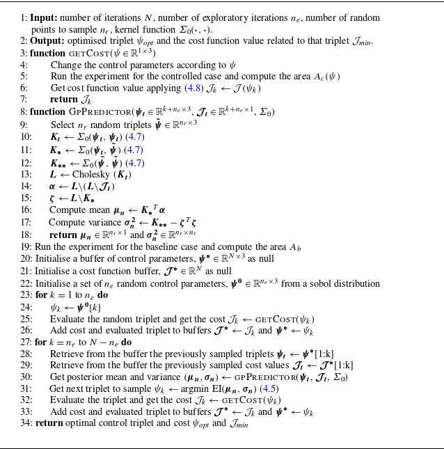
An initial exploration phase was conducted prior to optimisation, during which 32 points were sampled using the Sobol’ sequence (Sobol’ Reference Sobol’1967), a quasi-random low-discrepancy method. In summary, for each optimisation iteration, the posterior mean and variance are computed based on the outcomes of previous cost function evaluations; see (4.1). The acquisition function is then used to determine which triplet to sample in the current iteration according to (4.5). Once the selected triplet is identified, the actuation parameters are automatically adjusted. The function generator, which controls frequency and voltage amplitude, is controlled through a Python routine by using the PyVISA library. All the queries to the function generator are written with the rules and conventions of SCPI (standard commands for programmable instruments) language. Additionally, the BO interacts with the Arduino microcontroller to adjust the delay time, through a USB serial port. As well as for the signal generator, a Python routine was written to change the delay of the microcontroller. At the end of the iteration the cost function is evaluated (see (4.8)) and the next iteration is started. A further description, step-by-step, of the algorithm can be found in Appendix A.
5. Results and discussion
This section examines the optimisation results, emphasising three main aspects: the evaluation of the control parameters optimal triplet and the BO surrogate model in the input space, the influence of actuation parameters on the system response and the effects of control for the optimal conditions observed through conditional analysis.
5.1. Control parameters optimal triplet
The optimisation of the control parameters was performed with the rear probe positioned at $x^+ = 66$
and
$x^+ = 66$
and $y^+ =15$
. This position was chosen because it is sufficiently far away from the control point to avoid an influence of the vertical velocity component induced by the jet during the blowing phase, while still producing a pronounced control effect. After 150 iterations, the optimisation algorithm reached convergence in more than 5 h. From figure 10, it is observed that the lowest cost function value obtained was about
$y^+ =15$
. This position was chosen because it is sufficiently far away from the control point to avoid an influence of the vertical velocity component induced by the jet during the blowing phase, while still producing a pronounced control effect. After 150 iterations, the optimisation algorithm reached convergence in more than 5 h. From figure 10, it is observed that the lowest cost function value obtained was about $-54\,\%$
. By defining the reward value
$-54\,\%$
. By defining the reward value $R(\psi ) = - \mathcal{J}(\psi )$
, the maximum reward achieved was
$R(\psi ) = - \mathcal{J}(\psi )$
, the maximum reward achieved was $54\,\%$
. This value was achieved with the following optimised triplet for the control parameters (frequency, voltage amplitude and delay time, respectively):
$54\,\%$
. This value was achieved with the following optimised triplet for the control parameters (frequency, voltage amplitude and delay time, respectively):
 \begin{align} \psi _{\textit{opt}} = \left [ {60}\,\textrm {Hz}, {60}\,\textrm {mV}_{\textit{pp}}, {2.21}\,\textrm {ms} \right ]\!.\end{align}
The optimal triplet can be expressed in viscous units ( $\psi ^+_{\textit{opt}}$
) by using a viscous blowing period
$\psi ^+_{\textit{opt}}$
) by using a viscous blowing period $T^+_b$
(corresponding to half of the inverse of the actuation frequency
$T^+_b$
(corresponding to half of the inverse of the actuation frequency $f^+$
), a viscous delay time
$f^+$
), a viscous delay time $\Delta T^+$
and the maximum value of the jet wall-normal velocity
$\Delta T^+$
and the maximum value of the jet wall-normal velocity $V_{\textit{max}}^+$
in still air sampled at
$V_{\textit{max}}^+$
in still air sampled at $x^+=0$
and
$x^+=0$
and $y^+ =15$
(corresponding to a given combination of actuation frequency and voltage amplitude; see figure 8). The optimal control triplet scaled in viscous units is
$y^+ =15$
(corresponding to a given combination of actuation frequency and voltage amplitude; see figure 8). The optimal control triplet scaled in viscous units is
 \begin{align} \psi ^+_{\textit{opt}} = \left [ 13.83, 9.0, 3.62 \right ]\!, \end{align}
respectively $T^+_b$
,
$T^+_b$
, $V_{\textit{max}}^+$
and
$V_{\textit{max}}^+$
and $\Delta T^+$
. From the convergence plot of figure 10, we observe that a new minimum was discovered at iteration 146, following the previous local minimum identified by the BO algorithm at iteration 83. The local minimum found at iteration 83 was for the control triplet
$\Delta T^+$
. From the convergence plot of figure 10, we observe that a new minimum was discovered at iteration 146, following the previous local minimum identified by the BO algorithm at iteration 83. The local minimum found at iteration 83 was for the control triplet $\psi _{83} = [ {60}\,\textrm {Hz}, {69}\,\textrm {mV}_{\textit{pp}}, {3.02}\,\textrm {ms} ]$
or in viscous units
$\psi _{83} = [ {60}\,\textrm {Hz}, {69}\,\textrm {mV}_{\textit{pp}}, {3.02}\,\textrm {ms} ]$
or in viscous units $\psi ^+_{83} = [13.83, 9.8, 4.95 ]$
and led to a reward
$\psi ^+_{83} = [13.83, 9.8, 4.95 ]$
and led to a reward $R(\psi _{83}) = 53\,\%$
. Between iterations 83 and 146, the optimisation algorithm also found two other local minima with cost function values slightly higher than that for
$R(\psi _{83}) = 53\,\%$
. Between iterations 83 and 146, the optimisation algorithm also found two other local minima with cost function values slightly higher than that for $\psi _{83}$
. While we cannot guarantee that this value corresponds to the global minimum within the bounds specified in table 1, the results suggest that further improvements, if any, would likely require a significant number of iterations and yield only marginal reductions in the cost function compared with the minimum found at
$\psi _{83}$
. While we cannot guarantee that this value corresponds to the global minimum within the bounds specified in table 1, the results suggest that further improvements, if any, would likely require a significant number of iterations and yield only marginal reductions in the cost function compared with the minimum found at $\psi _{\textit{opt}}$
.
$\psi _{\textit{opt}}$
.

Figure 10. Minimum value for the cost function $\mathcal{J}(\psi )$
versus the iteration number.
$\mathcal{J}(\psi )$
versus the iteration number.
Figure 11 shows the effect of the control on the rear probe when positioned at $x^+ = 66$
and
$x^+ = 66$
and $y^+=15$
. The black line represents the baseline case and the blue line the controlled case with
$y^+=15$
. The black line represents the baseline case and the blue line the controlled case with $\psi _{\textit{opt}}$
. The area in grey represents the reduction in areas between the baseline and the controlled case. The first vertical dashed line, labelled with
$\psi _{\textit{opt}}$
. The area in grey represents the reduction in areas between the baseline and the controlled case. The first vertical dashed line, labelled with $t^*$
, indicates the instant in which the detection systems identify the sweep event from the front probe velocity signal, corresponding to
$t^*$
, indicates the instant in which the detection systems identify the sweep event from the front probe velocity signal, corresponding to $t=0$
. At this instant, the velocity time derivative turns out to be greater than the predetermined threshold (see § 3). Since the front and rear probes are positioned at two different streamwise coordinates, the second dashed vertical line marks the time,
$t=0$
. At this instant, the velocity time derivative turns out to be greater than the predetermined threshold (see § 3). Since the front and rear probes are positioned at two different streamwise coordinates, the second dashed vertical line marks the time, $t^*+ t_{\textit{corr}}$
, when the convected sweep event reaches the rear probe. The correlation time,
$t^*+ t_{\textit{corr}}$
, when the convected sweep event reaches the rear probe. The correlation time, $t^+_{\textit{corr}}$
, between the front and rear probes, was approximately
$t^+_{\textit{corr}}$
, between the front and rear probes, was approximately $9$
(see Appendix C). Moreover, it should be noted that the time at which the velocity starts to decrease in the controlled case corresponds to the sum of the delay time determined by the optimisation algorithm and the system response time. In addition, figure 11 shows that the time at which the velocity starts to decrease is not far from
$9$
(see Appendix C). Moreover, it should be noted that the time at which the velocity starts to decrease in the controlled case corresponds to the sum of the delay time determined by the optimisation algorithm and the system response time. In addition, figure 11 shows that the time at which the velocity starts to decrease is not far from $t^* + t_{\textit{corr}}$
. This observation highlights the effectiveness of the optimisation algorithm in adapting the delay time to achieve maximum reward, despite the absence of prior information regarding the correlation time. As a comparison, Rebbeck & Choi (Reference Rebbeck and Choi2006) in their experiment actuated at the instant corresponding to
$t^* + t_{\textit{corr}}$
. This observation highlights the effectiveness of the optimisation algorithm in adapting the delay time to achieve maximum reward, despite the absence of prior information regarding the correlation time. As a comparison, Rebbeck & Choi (Reference Rebbeck and Choi2006) in their experiment actuated at the instant corresponding to $t^* + t_{\textit{corr}}$
.
$t^* + t_{\textit{corr}}$
.

Figure 11. Conditionally averaged sweep events computed with the signal of the rear probe ( $x^+ = 66$
and
$x^+ = 66$
and $y^+ = 15$
). The actuation control triplet is the optimal one (
$y^+ = 15$
). The actuation control triplet is the optimal one ( $\psi _{\textit{opt}}$
). The first dashed line indicates the instant
$\psi _{\textit{opt}}$
). The first dashed line indicates the instant $t^*$
in which the sweep event is detected. The second dashed line indicates the instant
$t^*$
in which the sweep event is detected. The second dashed line indicates the instant $t^* + t_{\textit{corr}}$
when the convected sweep event reaches the rear probe.
$t^* + t_{\textit{corr}}$
when the convected sweep event reaches the rear probe.
In order to attempt a comparison between the wall-normal velocity generated by the jet for the optimal conditions and the wall-normal velocity component of the sweep event, it is first necessary to acknowledge that the wall-normal velocity of the jet in still air is significantly attenuated due to its interaction with the cross-flow. According to the particle image velocimetry measurements reported by Klotz, Gumowski & Wesfreid (Reference Klotz, Gumowski and Wesfreid2019), a continuous jet in cross-flow with a velocity ratio VR $ \in [0.5, 0.7]$
and Reynolds number
$ \in [0.5, 0.7]$
and Reynolds number $\textit{Re}_D = 310$
undergoes an approximate 75 % reduction in wall-normal velocity at
$\textit{Re}_D = 310$
undergoes an approximate 75 % reduction in wall-normal velocity at $y/D_{\textit{jet}} = 1.5$
compared with the velocity at the jet exit plane (
$y/D_{\textit{jet}} = 1.5$
compared with the velocity at the jet exit plane ( $y/D_{\textit{jet}} = 0$
). Here, the velocity ratio VR is defined as the ratio between the jet exit velocity,
$y/D_{\textit{jet}} = 0$
). Here, the velocity ratio VR is defined as the ratio between the jet exit velocity, $V_{\textit{jet}}$
, and the free-stream velocity,
$V_{\textit{jet}}$
, and the free-stream velocity, $U_{\!f}$
, while the Reynolds number
$U_{\!f}$
, while the Reynolds number $\textit{Re}_D$
is based on the jet diameter,
$\textit{Re}_D$
is based on the jet diameter, $D_{\textit{jet}}$
, and the free-stream velocity. It should be pointed out that in our experiment, the jet issuing from the jet orifice is not continuous as in the case of the jet used by Klotz et al. (Reference Klotz, Gumowski and Wesfreid2019). However, the two experiments share comparable non-dimensional parameters: the velocity ratio in our experiment was approximately
$D_{\textit{jet}}$
, and the free-stream velocity. It should be pointed out that in our experiment, the jet issuing from the jet orifice is not continuous as in the case of the jet used by Klotz et al. (Reference Klotz, Gumowski and Wesfreid2019). However, the two experiments share comparable non-dimensional parameters: the velocity ratio in our experiment was approximately $0.5$
(using
$0.5$
(using $V_{\textit{max}}^+ \approx 10$
as the maximum wall-normal jet velocity) and the Reynolds number based on
$V_{\textit{max}}^+ \approx 10$
as the maximum wall-normal jet velocity) and the Reynolds number based on $U_0$
and
$U_0$
and $d$
was approximately
$d$
was approximately $200$
. Under this assumption, the estimated wall-normal velocity in viscous units produced by the jet in cross-flow at
$200$
. Under this assumption, the estimated wall-normal velocity in viscous units produced by the jet in cross-flow at $y^+=15$
(corresponding to
$y^+=15$
(corresponding to $y/d = 1.5$
) is close to
$y/d = 1.5$
) is close to $2.5$
. This value is close to the average wall-normal velocity observed during the downwash of sweep events, which is approximately
$2.5$
. This value is close to the average wall-normal velocity observed during the downwash of sweep events, which is approximately $2$
as reported by Lozano-Durán et al. (Reference Lozano-Durán, Flores and Jiménez2012) .
$2$
as reported by Lozano-Durán et al. (Reference Lozano-Durán, Flores and Jiménez2012) .
Lozano-Durán & Jiménez (Reference Lozano-Durán and Jiménez2014) by tracking in time coherent structures in a turbulent channel flow found that the lifetime of sweep and ejection events in the buffer layer, defined as their time elapsed between the first and the last appearance, is approximately $30$
viscous times. This time scale is notably longer than the optimal blowing period (
$30$
viscous times. This time scale is notably longer than the optimal blowing period ( $T^+_b \approx 14$
) identified in the present study, which corresponds to the upper limit of the explored range. As discussed before, it can not be extended further due to technical constraints. Given this observation, we hypothesise that longer actuation periods allow a greater control coverage of the sweep events and may result in higher reward values.
$T^+_b \approx 14$
) identified in the present study, which corresponds to the upper limit of the explored range. As discussed before, it can not be extended further due to technical constraints. Given this observation, we hypothesise that longer actuation periods allow a greater control coverage of the sweep events and may result in higher reward values.
Probability density functions of the fluctuating streamwise velocity signal, conditioned on sweep events, are shown in figure 12 for both the baseline and the controlled case with $\psi _{\textit{opt}}$
. Probability density functions were computed for a position corresponding to
$\psi _{\textit{opt}}$
. Probability density functions were computed for a position corresponding to $x^+=66$
and
$x^+=66$
and $y^ +=15$
using a kernel density estimator (KDE) (Silverman Reference Silverman2018; Waskom Reference Waskom2021). The effect of the control is clearly visible in the left tail of the distribution, with more pronounced negative values compared with the baseline case. In contrast, weakly positive fluctuations exhibit a lower probability. This behaviour can be attributed to the fluctuations imposed by the coherent component introduced by the jet, which alters the dynamics of the natural sweep event (see also the discussion in § 5.4.3 regarding the wavelet spectra). Based on these considerations, it can be hypothesised that the control is able to alter the turbulence regeneration mechanisms by introducing artificial ejection events. This interpretation is consistent with the more negative skewness values characterising the conditional PDF observed in the controlled case (
$y^ +=15$
using a kernel density estimator (KDE) (Silverman Reference Silverman2018; Waskom Reference Waskom2021). The effect of the control is clearly visible in the left tail of the distribution, with more pronounced negative values compared with the baseline case. In contrast, weakly positive fluctuations exhibit a lower probability. This behaviour can be attributed to the fluctuations imposed by the coherent component introduced by the jet, which alters the dynamics of the natural sweep event (see also the discussion in § 5.4.3 regarding the wavelet spectra). Based on these considerations, it can be hypothesised that the control is able to alter the turbulence regeneration mechanisms by introducing artificial ejection events. This interpretation is consistent with the more negative skewness values characterising the conditional PDF observed in the controlled case ( $-0.56$
) compared with the baseline case (
$-0.56$
) compared with the baseline case ( $-0.39$
). This also aligns with observations of Kim, Moin & Moser (Reference Kim, Moin and Moser1987) for the canonical case, where regions dominated by ejections correspond to more negative skewness values with respect to regions dominated by sweeps.
$-0.39$
). This also aligns with observations of Kim, Moin & Moser (Reference Kim, Moin and Moser1987) for the canonical case, where regions dominated by ejections correspond to more negative skewness values with respect to regions dominated by sweeps.

Figure 12. Conditional PDFs of the streamwise velocity component, obtained through KDE in the baseline case and in the controlled case ( $\psi _{\textit{opt}}$
). Here
$\psi _{\textit{opt}}$
). Here $x^+=66$
and
$x^+=66$
and $y^+=15$
.
$y^+=15$
.
5.2. Surrogate model evaluation in the input space
As discussed in § 4, the BO algorithm relies on constructing a surrogate model for the cost function within the input space. This section presents and analyses the results of that process. While in § 5.3 we focus on how the system responds to changes in the actuation parameters by analysing the conditionally averaged event at the rear probe, in § 5.2 we evaluate the posterior mean of the surrogate model. The posterior mean provides a close approximation of the cost function after all the iterations, offering a more refined view of the system behaviour based on the actuation parameters, and was evaluated as shown in (4.2) to provide insights into the distribution of the cost function. Understanding this distribution is very important, not just to guide exploration toward an ever-improving minimum but also to understand how changes in the input parameters influence the system performances, and thus helping to identify regions where optimal solutions are most likely to be found.
The posterior mean, $\mu _n$
, is depicted as a function of delay time and frequency with a fixed voltage amplitude
$\mu _n$
, is depicted as a function of delay time and frequency with a fixed voltage amplitude $\hat {A} = {60}\,\textrm {mV}_{\textit{pp}}$
in figure 13(a), and as a function of delay time and voltage amplitude with a constant frequency
$\hat {A} = {60}\,\textrm {mV}_{\textit{pp}}$
in figure 13(a), and as a function of delay time and voltage amplitude with a constant frequency $f={60}\,\textrm {Hz}$
in figure 13(b). The cost function minimum found in § 5.1 is clearly visible in both figures 13(a) and 13(b) leading to a reward of
$f={60}\,\textrm {Hz}$
in figure 13(b). The cost function minimum found in § 5.1 is clearly visible in both figures 13(a) and 13(b) leading to a reward of $54\,\%$
. What emerges most from this analysis is that lowering the frequency across the input space leads to a notable reduction in the cost function, resulting in an increased reward. Specifically,
$54\,\%$
. What emerges most from this analysis is that lowering the frequency across the input space leads to a notable reduction in the cost function, resulting in an increased reward. Specifically, $\mu _n$
values drop from about
$\mu _n$
values drop from about $-30 \,\%$
at higher frequencies to around
$-30 \,\%$
at higher frequencies to around $-45 \,\%$
in the frequency range from
$-45 \,\%$
in the frequency range from $60$
to
$60$
to ${65}\,\textrm {Hz}$
, highlighting the significant impact of frequency adjustment in improving performances. For frequencies below
${65}\,\textrm {Hz}$
, highlighting the significant impact of frequency adjustment in improving performances. For frequencies below ${65}\,\textrm {Hz}$
, fine tuning the delay time further reduces the cost function. This suggests that while frequency drives the primary effect, optimising the delay time provides a critical adjustment to improve the outcomes. There is generally an improvement for low delay times even for higher frequencies, up to
${65}\,\textrm {Hz}$
, fine tuning the delay time further reduces the cost function. This suggests that while frequency drives the primary effect, optimising the delay time provides a critical adjustment to improve the outcomes. There is generally an improvement for low delay times even for higher frequencies, up to ${75}\,\textrm {Hz}$
. This effect can also be observed in figure 13(b), where all the minima and areas exhibiting lower
${75}\,\textrm {Hz}$
. This effect can also be observed in figure 13(b), where all the minima and areas exhibiting lower $\mu _n$
are observed for
$\mu _n$
are observed for $\Delta T$
less than
$\Delta T$
less than ${3.5}\,\textrm {ms}$
. Although a fairly monotonic behaviour can be observed for the frequency, it is not the same for the voltage amplitude. Indeed, as can be seen in figure 13(b), there are numerous minima for different voltage amplitude values. For these local minima, a posterior standard deviation value of
${3.5}\,\textrm {ms}$
. Although a fairly monotonic behaviour can be observed for the frequency, it is not the same for the voltage amplitude. Indeed, as can be seen in figure 13(b), there are numerous minima for different voltage amplitude values. For these local minima, a posterior standard deviation value of $0.5\,\%$
was found. This indicates low uncertainty in the regions corresponding to the lowest cost function value. This behaviour is consistent with the expected negative correlation between posterior mean and posterior standard deviation arising in BO: regions that exhibit low posterior mean (high reward) tend to be sampled more extensively, which naturally reduces their uncertainty. Conversely, areas where the posterior mean is far from the minimum are explored less and, thus, are characterised by higher uncertainty.
$0.5\,\%$
was found. This indicates low uncertainty in the regions corresponding to the lowest cost function value. This behaviour is consistent with the expected negative correlation between posterior mean and posterior standard deviation arising in BO: regions that exhibit low posterior mean (high reward) tend to be sampled more extensively, which naturally reduces their uncertainty. Conversely, areas where the posterior mean is far from the minimum are explored less and, thus, are characterised by higher uncertainty.

Figure 13. (a) Posterior mean $\mu _n$
in percentage presented as a function of the delay time
$\mu _n$
in percentage presented as a function of the delay time $\Delta T$
and the frequency
$\Delta T$
and the frequency $f$
by keeping the voltage amplitude set to
$f$
by keeping the voltage amplitude set to $\hat {A} = {60}\,\textrm {mV}_{\textit{pp}}$
; (b) posterior mean
$\hat {A} = {60}\,\textrm {mV}_{\textit{pp}}$
; (b) posterior mean $\mu _n$
in percentage depicted as a function of
$\mu _n$
in percentage depicted as a function of $\Delta T$
and
$\Delta T$
and $\hat {A}$
by keeping the frequency set to
$\hat {A}$
by keeping the frequency set to $f={60}\,\textrm {Hz}$
.
$f={60}\,\textrm {Hz}$
.
5.3. Influence of actuation parameters on the system response
It is worth observing how the system responds to changes in the actuation parameters, as these adjustments can significantly impact the overall behaviour. Three distinct test cases were selected to assess system sensitivity, each designed to isolate the effects of each single control parameter on the system response. The complete set of control triplets in dimensional units and their corresponding values in viscous units are reported in table 2. For clarity, the triplets have been labelled from $\psi _1$
to
$\psi _1$
to $\psi _4$
, to facilitate their identification throughout the analysis. Figure 15 depicts the jet wall-normal velocity in still air sampled at
$\psi _4$
, to facilitate their identification throughout the analysis. Figure 15 depicts the jet wall-normal velocity in still air sampled at $x^+=0$
and
$x^+=0$
and $y^+=15$
for the control triplets of table 2.
$y^+=15$
for the control triplets of table 2.
Table 2. Control triplets in dimensional units and their corresponding values in viscous units employed in § 5.3.

In figure 14(a) the effect of the actuation frequency can be observed. Two test cases, namely $\psi _{\textit{opt}}$
and
$\psi _{\textit{opt}}$
and $\psi _1$
, characterised by the same voltage amplitude (
$\psi _1$
, characterised by the same voltage amplitude ( $\hat {A} = {60}\,\textrm {mV}_{\textit{pp}}$
) and delay time (
$\hat {A} = {60}\,\textrm {mV}_{\textit{pp}}$
) and delay time ( $\Delta T = {2.20}\,\textrm {ms}$
) but different actuation frequencies (
$\Delta T = {2.20}\,\textrm {ms}$
) but different actuation frequencies ( $f_1 = {60}\,\textrm {Hz}$
and
$f_1 = {60}\,\textrm {Hz}$
and $f_2 = {100}\,\textrm {Hz}$
) are compared. It is evident that the lower actuation frequency results in a longer actuation period (from
$f_2 = {100}\,\textrm {Hz}$
) are compared. It is evident that the lower actuation frequency results in a longer actuation period (from $T^+=8.40$
to
$T^+=8.40$
to $T^+=13.83$
), thereby allowing for greater streamwise coverage of the opposition control and more significant reductions in the longitudinal velocity component associated with the sweep event (Rebbeck & Choi Reference Rebbeck and Choi2006). In addition, a marked reduction in velocity is also observed for the triplet corresponding to
$T^+=13.83$
), thereby allowing for greater streamwise coverage of the opposition control and more significant reductions in the longitudinal velocity component associated with the sweep event (Rebbeck & Choi Reference Rebbeck and Choi2006). In addition, a marked reduction in velocity is also observed for the triplet corresponding to $\psi _{\textit{opt}}$
compared with that of
$\psi _{\textit{opt}}$
compared with that of $\psi _1$
. This is due to the fact that the response of the jet actuator is not linear and, as can also be observed in figure 15, a change in frequency can also change the value of
$\psi _1$
. This is due to the fact that the response of the jet actuator is not linear and, as can also be observed in figure 15, a change in frequency can also change the value of $V_{\textit{max}}^+$
. In this case, for the triplet
$V_{\textit{max}}^+$
. In this case, for the triplet $\psi _1$
, the value of
$\psi _1$
, the value of $V_{\textit{max}}^+$
turns out to be higher than that of
$V_{\textit{max}}^+$
turns out to be higher than that of $\psi _{\textit{opt}}$
. This behaviour is further analysed in figure 14(b), which compares two control triplets,
$\psi _{\textit{opt}}$
. This behaviour is further analysed in figure 14(b), which compares two control triplets, $\psi _{\textit{opt}}$
and
$\psi _{\textit{opt}}$
and $\psi _2$
, with voltage amplitudes of
$\psi _2$
, with voltage amplitudes of ${60}\,\textrm {mV}_{\textit{pp}}$
and
${60}\,\textrm {mV}_{\textit{pp}}$
and ${71}\,\textrm {mV}_{\textit{pp}}$
, respectively, while keeping the frequency and the delay time fixed to
${71}\,\textrm {mV}_{\textit{pp}}$
, respectively, while keeping the frequency and the delay time fixed to $f = {60}\,\textrm {Hz}$
and
$f = {60}\,\textrm {Hz}$
and $\Delta T = {2.20}\,\textrm {ms}$
. Although
$\Delta T = {2.20}\,\textrm {ms}$
. Although $\psi _2$
yields a higher maximum wall-normal velocity (
$\psi _2$
yields a higher maximum wall-normal velocity ( $V_{\textit{max}}^+ = 10.0$
) than
$V_{\textit{max}}^+ = 10.0$
) than $\psi _{\textit{opt}}$
(
$\psi _{\textit{opt}}$
( $V_{\textit{max}}^+ = 9.0$
), the latter results in a more pronounced velocity reduction. This behaviour can be explained by the fact that, if the jet intensity exceeds the optimal value, the vertical velocity component of the sweep event is not properly counteracted, thereby resulting in limited effectiveness of the control (see § 5.1). Figure 14(c) shows how the delay time imposed through the microcontroller causes the velocity reduction to be anticipated or delayed by keeping constant frequency (
$V_{\textit{max}}^+ = 9.0$
), the latter results in a more pronounced velocity reduction. This behaviour can be explained by the fact that, if the jet intensity exceeds the optimal value, the vertical velocity component of the sweep event is not properly counteracted, thereby resulting in limited effectiveness of the control (see § 5.1). Figure 14(c) shows how the delay time imposed through the microcontroller causes the velocity reduction to be anticipated or delayed by keeping constant frequency ( $f={60}\,\textrm {Hz}$
) and voltage amplitude (
$f={60}\,\textrm {Hz}$
) and voltage amplitude ( $\hat {A} = {60}\,\textrm {mV}_{\textit{pp}}$
). A high delay (
$\hat {A} = {60}\,\textrm {mV}_{\textit{pp}}$
). A high delay ( $\Delta T = {5.70}\,\textrm {ms}$
) allows reductions to occur when the velocity is the highest; conversely, a reduced delay (
$\Delta T = {5.70}\,\textrm {ms}$
) allows reductions to occur when the velocity is the highest; conversely, a reduced delay ( $\Delta T = {1.01}\,\textrm {ms}$
) prevents the onset of the velocity peak observable in the baseline case. Moreover, a comparison between the brown line (
$\Delta T = {1.01}\,\textrm {ms}$
) prevents the onset of the velocity peak observable in the baseline case. Moreover, a comparison between the brown line ( $\Delta T = {1.01}\,\textrm {ms}$
) and the blue line (
$\Delta T = {1.01}\,\textrm {ms}$
) and the blue line ( $\Delta T = {2.21}\,\textrm {ms}$
, corresponding to the delay of the optimal triplet
$\Delta T = {2.21}\,\textrm {ms}$
, corresponding to the delay of the optimal triplet $\psi _{\textit{opt}}$
), reveals that an actuation occurring close to
$\psi _{\textit{opt}}$
), reveals that an actuation occurring close to $t^* + t_{\textit{corr}}$
, as implemented in the work of Rebbeck & Choi (Reference Rebbeck and Choi2006), is less effective than a slightly delayed actuation. This is due to the fact that, in the present experiment, the maximum blowing duration is shorter than that used by Rebbeck & Choi (Reference Rebbeck and Choi2006). As a consequence, the optimisation algorithm tends to delay the actuation to align the blowing phase with the region of maximum intensity of the sweep event.
$t^* + t_{\textit{corr}}$
, as implemented in the work of Rebbeck & Choi (Reference Rebbeck and Choi2006), is less effective than a slightly delayed actuation. This is due to the fact that, in the present experiment, the maximum blowing duration is shorter than that used by Rebbeck & Choi (Reference Rebbeck and Choi2006). As a consequence, the optimisation algorithm tends to delay the actuation to align the blowing phase with the region of maximum intensity of the sweep event.

Figure 14. Actuation parameters influence on the system response. (a) Blowing period influence; (b) jet velocity amplitude influence; (c) delay time influence. The black dashed line indicates the conditionally averaged sweep events for the fluctuating velocity $u^+$
in the baseline case. Coloured curves indicate the conditionally averaged sweep event for different control triplets
$u^+$
in the baseline case. Coloured curves indicate the conditionally averaged sweep event for different control triplets $\psi _i$
(see table 2).
$\psi _i$
(see table 2).

Figure 15. Actuation parameters influence on the jet vertical wall-normal velocity in still air at $x^+=0$
and
$x^+=0$
and $y^+=15$
for different control triplets
$y^+=15$
for different control triplets $\psi _i$
.
$\psi _i$
.
Further discussion of the influence of the actuation parameters on the system response through the analysis of energy spectra has been carried out in Appendix B.
5.4. Control effects for the optimal triplet observed through conditional analysis
The implementation of a conditional analysis highlighted the effect of the control, allowing for a more effective comparison with the baseline case. As previously pointed out, the optimisation of the control parameters was performed with the rear probe positioned at $x^+ = 66$
and
$x^+ = 66$
and $y^+ =15$
. However, it is relevant to observe the effects of the control further downstream and upstream of the position chosen for the optimisation. Measurements at different streamwise locations were performed to characterise the modifications in the flow behaviour when the control was active.
$y^+ =15$
. However, it is relevant to observe the effects of the control further downstream and upstream of the position chosen for the optimisation. Measurements at different streamwise locations were performed to characterise the modifications in the flow behaviour when the control was active.
5.4.1. Conditionally averaged sweep events
Figure 16 illustrates the longitudinal velocity component of the conditionally averaged sweep events as a function of time in viscous units at various streamwise coordinates, comparing the baseline and controlled case. In the controlled case, the actuation parameters are set to the optimal values, denoted by $\psi _{\textit{opt}}$
. From figure 16(a–d) sweep events are represented at four different streamwise distances. A comparison of the sweep events at the optimisation point (
$\psi _{\textit{opt}}$
. From figure 16(a–d) sweep events are represented at four different streamwise distances. A comparison of the sweep events at the optimisation point ( $x^+ = 66$
) and a position closer to the jet orifice (
$x^+ = 66$
) and a position closer to the jet orifice ( $x^+ = 45$
) reveals similar control effects. Moving downstream from the optimisation point to
$x^+ = 45$
) reveals similar control effects. Moving downstream from the optimisation point to $x^+ = 419$
, a progressive reduction in the intensity of the events is observed in both the baseline and controlled cases. Moreover, the effect of the control gradually weakens along the streamwise direction and becomes negligible at distances of about
$x^+ = 419$
, a progressive reduction in the intensity of the events is observed in both the baseline and controlled cases. Moreover, the effect of the control gradually weakens along the streamwise direction and becomes negligible at distances of about $400$
viscous units.
$400$
viscous units.

Figure 16. Conditionally averaged sweep events at different streamwise distances, $x^+$
, and constant wall-normal distance
$x^+$
, and constant wall-normal distance $y^+=15$
for the baseline and the controlled case. Results are shown for (a)
$y^+=15$
for the baseline and the controlled case. Results are shown for (a) $x^+=45$
, (b)
$x^+=45$
, (b) $x^+=66$
, (c)
$x^+=66$
, (c) $x^+=116$
, (d)
$x^+=116$
, (d) $x^+=419$
. (e) Baseline conditionally averaged sweep events interpolated across different
$x^+=419$
. (e) Baseline conditionally averaged sweep events interpolated across different $x^+$
distances; ( f) controlled conditionally averaged sweep events interpolated across different
$x^+$
distances; ( f) controlled conditionally averaged sweep events interpolated across different $x^+$
distances.
$x^+$
distances.
In figure 16(e, f) the conditionally averaged sweep events are interpolated with a cubic function for all the observed streamwise distances (12 different distances from $x^+ = 25$
to
$x^+ = 25$
to $x^+=419$
). Figures 16(e) and 16( f) represent the baseline and controlled test case, respectively. In the controlled case, a pronounced velocity reduction zone is visible, extending approximately 150 viscous units downstream from the actuation point. When comparing figures 16(e) and 16( f), it is observed that in the controlled case, a more pronounced velocity reduction is present for times earlier than the front probe detection time (
$x^+=419$
). Figures 16(e) and 16( f) represent the baseline and controlled test case, respectively. In the controlled case, a pronounced velocity reduction zone is visible, extending approximately 150 viscous units downstream from the actuation point. When comparing figures 16(e) and 16( f), it is observed that in the controlled case, a more pronounced velocity reduction is present for times earlier than the front probe detection time ( $t^+=0$
). The velocity reduction starting from
$t^+=0$
). The velocity reduction starting from $t^+ \lt 0$
in the baseline case is a signature of the natural evolution of the sweep event. On the other hand, the more pronounced effect in the controlled case arises because, sometimes, the temporal interval between successive events is shorter than the width of the conditionally averaging temporal window, allowing multiple control effects to be captured within a single window.
$t^+ \lt 0$
in the baseline case is a signature of the natural evolution of the sweep event. On the other hand, the more pronounced effect in the controlled case arises because, sometimes, the temporal interval between successive events is shorter than the width of the conditionally averaging temporal window, allowing multiple control effects to be captured within a single window.
5.4.2. Conditionally averaged cross-correlation function
The conditional cross-correlation function between the front and the rear probe fluctuating velocity signal is computed here. The cross-correlation between two known real signals, $x(t)$
and
$x(t)$
and $y(t)$
, can be defined as
$y(t)$
, can be defined as
 \begin{equation} R_{\textit{xy}}(\tau ) = \int _{0}^{T} x(t)y(t+\tau )\, {\rm d}t, \end{equation}
where $\tau$
is the time lag and
$\tau$
is the time lag and $T$
is the signal length. The cross-correlation function conditionally averaged over sweep events was computed as
$T$
is the signal length. The cross-correlation function conditionally averaged over sweep events was computed as
 \begin{equation} \langle R_{\textit{xy}}(\tau )\rangle = \frac {1}{N}\sum _{n=0}^N R_{x_ny_n}(\tau ), \end{equation}
where $N$
is the total number of detected sweep events. The subscript
$N$
is the total number of detected sweep events. The subscript $n$
indicates a 400-sample window (
$n$
indicates a 400-sample window ( $\tau ^+ \approx 65$
) of the signal centred with respect to the raising edge of the trigger generated when the sweep event is detected (§ 3). The conditionally averaged cross-correlation coefficient was defined as
$\tau ^+ \approx 65$
) of the signal centred with respect to the raising edge of the trigger generated when the sweep event is detected (§ 3). The conditionally averaged cross-correlation coefficient was defined as
 \begin{equation} \langle \rho _{\textit{xy}}(\tau )\rangle = {\frac {\langle R_{\textit{xy}} (\tau )\rangle }{\sqrt { \langle R_{xx} (0) \rangle \langle R_{yy}(0) \rangle }}}, \end{equation}
where $R_{xx} (0)$
and
$R_{xx} (0)$
and $R_{yy} (0)$
indicate the value of the autocorrelation function of both signals at zero time lag.
$R_{yy} (0)$
indicate the value of the autocorrelation function of both signals at zero time lag.
Figure 17 depicts the conditionally averaged cross-correlation coefficient, $\langle \rho _{u_{\!f} u_r}\rangle$
, of the fluctuating velocity signals coming from the front,
$\langle \rho _{u_{\!f} u_r}\rangle$
, of the fluctuating velocity signals coming from the front, $u_{\!f}$
, and the rear probe,
$u_{\!f}$
, and the rear probe, $u_r$
, as a function of the time lag,
$u_r$
, as a function of the time lag, $\tau ^+$
, for both the baseline and controlled case. It is important to highlight that, in the controlled case, the evolution of the sweep event can be essentially divided into two distinct phases: one before the control effects take place and one after. By analysing the cross-correlation function we can observe that the maximum values for both the baseline and the controlled case are crossed by the same vertical dashed line, which is positioned in correspondence of
$\tau ^+$
, for both the baseline and controlled case. It is important to highlight that, in the controlled case, the evolution of the sweep event can be essentially divided into two distinct phases: one before the control effects take place and one after. By analysing the cross-correlation function we can observe that the maximum values for both the baseline and the controlled case are crossed by the same vertical dashed line, which is positioned in correspondence of $\tau ^+ \approx 9$
. This fact indicates that the convection time of the sweep event in the baseline case does not significantly differ from the convection time of the sweep event in the controlled case during the initial phase. It can also be noted that this value is nearly identical to the one computed without applying any conditioning to the baseline signal (refer to the value of
$\tau ^+ \approx 9$
. This fact indicates that the convection time of the sweep event in the baseline case does not significantly differ from the convection time of the sweep event in the controlled case during the initial phase. It can also be noted that this value is nearly identical to the one computed without applying any conditioning to the baseline signal (refer to the value of $t^+_{\textit{corr}}$
evaluated in Appendix C for
$t^+_{\textit{corr}}$
evaluated in Appendix C for $x^+=66$
), indicating that the conditionally averaged convection velocity of the sweep events in the baseline case aligns with the convection velocity averaged all over the times. The occurrence of a secondary cross-correlation peak in the controlled case is observable in figure 17. This secondary peak, related to the second phase of the sweep event in the controlled case, appears at a time lag of
$x^+=66$
), indicating that the conditionally averaged convection velocity of the sweep events in the baseline case aligns with the convection velocity averaged all over the times. The occurrence of a secondary cross-correlation peak in the controlled case is observable in figure 17. This secondary peak, related to the second phase of the sweep event in the controlled case, appears at a time lag of $\tau ^+ \approx 18$
, which corresponds to the temporal separation between the velocity minimum observed during the sweep event detected by the front probe and the subsequent velocity minimum associated with the controlled sweep event produced during the jet-blowing phase. It is also observed that the control mechanism reduces the cross-correlation value of the first peak compared with the baseline case. This phenomenon arises because, in the controlled case, the control modifies the structure of the natural sweep event detected by the front probe, leading to an inevitable reduction in the cross-correlation between the signals measured by the front and rear probe.
$\tau ^+ \approx 18$
, which corresponds to the temporal separation between the velocity minimum observed during the sweep event detected by the front probe and the subsequent velocity minimum associated with the controlled sweep event produced during the jet-blowing phase. It is also observed that the control mechanism reduces the cross-correlation value of the first peak compared with the baseline case. This phenomenon arises because, in the controlled case, the control modifies the structure of the natural sweep event detected by the front probe, leading to an inevitable reduction in the cross-correlation between the signals measured by the front and rear probe.

Figure 17. Conditional cross-correlation coefficient between the fluctuating component of the velocity sampled from the front probe positioned at $x^+=-55, y^+ =15$
and the rear probe positioned at
$x^+=-55, y^+ =15$
and the rear probe positioned at $x^+=66, y^+ =15$
as a function of the time lag,
$x^+=66, y^+ =15$
as a function of the time lag, $\tau ^+$
. The vertical dashed line marks the position (
$\tau ^+$
. The vertical dashed line marks the position ( $\tau ^+ \approx 9$
) of the maximum values of the cross-correlation function for both the baseline and the controlled case.
$\tau ^+ \approx 9$
) of the maximum values of the cross-correlation function for both the baseline and the controlled case.
To compare the convective velocity during the two phases of the controlled sweep event, the conditional cross-correlation function between the front and rear probe at two different streamwise distances ( $x^+=45$
and
$x^+=45$
and $x^+ = 66$
) was depicted in figure 18. The time lag difference between the first peaks of the cross-correlation functions is denoted by
$x^+ = 66$
) was depicted in figure 18. The time lag difference between the first peaks of the cross-correlation functions is denoted by $\Delta \tau ^+_1$
and is approximately
$\Delta \tau ^+_1$
and is approximately $1.5$
viscous units. This value leads to a convection velocity, related to the first phase of the sweep event, of about
$1.5$
viscous units. This value leads to a convection velocity, related to the first phase of the sweep event, of about $14$
viscous units. The time lag difference of the secondary peaks of the cross-correlation functions is indicated with
$14$
viscous units. The time lag difference of the secondary peaks of the cross-correlation functions is indicated with $\Delta \tau ^+_2$
and is equivalent to about
$\Delta \tau ^+_2$
and is equivalent to about $2.1$
viscous units. The convection velocity of the sweep event during the second phase is about
$2.1$
viscous units. The convection velocity of the sweep event during the second phase is about $10$
viscous units. This highlights the huge reduction of the sweep event convection velocity during the blowing phase of the jet. A general decrease in the values characterising the conditionally averaged cross-correlation function is also observed at
$10$
viscous units. This highlights the huge reduction of the sweep event convection velocity during the blowing phase of the jet. A general decrease in the values characterising the conditionally averaged cross-correlation function is also observed at $x^+ = 66$
compared with those at
$x^+ = 66$
compared with those at $x^+ = 45$
. This reduction is attributed to the natural loss of correlation when the distance between the front and rear probe is increased.
$x^+ = 45$
. This reduction is attributed to the natural loss of correlation when the distance between the front and rear probe is increased.

Figure 18. Conditional cross-correlation coefficient between the fluctuating component of the velocity sampled from the front probe positioned at $x^+=-55, y^+ =15$
and the rear probe positioned at two different streamwise distances (indicated in the legend) as a function of the time lag,
$x^+=-55, y^+ =15$
and the rear probe positioned at two different streamwise distances (indicated in the legend) as a function of the time lag, $\tau ^+$
. Both continuous lines represent the controlled case. The four dashed lines indicate the function maxima. Here
$\tau ^+$
. Both continuous lines represent the controlled case. The four dashed lines indicate the function maxima. Here $\Delta \tau ^+_1$
is the time lag difference between the first two peaks;
$\Delta \tau ^+_1$
is the time lag difference between the first two peaks; $\Delta \tau ^+_2$
is the time lag difference between the second two peaks.
$\Delta \tau ^+_2$
is the time lag difference between the second two peaks.
5.4.3. Conditionally averaged energy spectra
In this section the conditional analysis was extended to the energy spectra. The fluctuating velocity signal of the rear probe was divided into windows of $2^{10}$
elements with a period approximately of
$2^{10}$
elements with a period approximately of $168$
viscous units, each containing a sweep event identified by the detection system; see § 3. The one-sided energy spectrum,
$168$
viscous units, each containing a sweep event identified by the detection system; see § 3. The one-sided energy spectrum, $\phi _{uu}(f)$
, at a fixed wall-normal location
$\phi _{uu}(f)$
, at a fixed wall-normal location $y^+=15$
was computed for each window and ensemble averaged. The conditional averaged energy spectrum can be denoted as
$y^+=15$
was computed for each window and ensemble averaged. The conditional averaged energy spectrum can be denoted as $\langle \phi _{uu}(f) \rangle$
. The resulting spectral resolution was
$\langle \phi _{uu}(f) \rangle$
. The resulting spectral resolution was $\Delta f={9.76}\,\textrm {Hz}$
and each window underwent a Hanning windowing procedure (Oppenheim & Schafer Reference Oppenheim and Schafer1989). At the end, energy spectra were premultiplied and inner scaled, yielding
$\Delta f={9.76}\,\textrm {Hz}$
and each window underwent a Hanning windowing procedure (Oppenheim & Schafer Reference Oppenheim and Schafer1989). At the end, energy spectra were premultiplied and inner scaled, yielding $f^+ \langle \phi _{uu}^+(f) \rangle$
. Figure 19 presents the inner-scaled premultiplied conditionally averaged energy spectra at
$f^+ \langle \phi _{uu}^+(f) \rangle$
. Figure 19 presents the inner-scaled premultiplied conditionally averaged energy spectra at $y^+ = 15$
and different streamwise locations (
$y^+ = 15$
and different streamwise locations ( $x^+ = 45, x^+ = 66, x^+ = 419$
). It can be observed that the control produces a broadband increase of fluctuating kinetic energy for the streamwise locations near the actuator (
$x^+ = 45, x^+ = 66, x^+ = 419$
). It can be observed that the control produces a broadband increase of fluctuating kinetic energy for the streamwise locations near the actuator ( $x^+ = 45, x^+ = 66$
), while no substantial differences between the baseline and the controlled case for
$x^+ = 45, x^+ = 66$
), while no substantial differences between the baseline and the controlled case for $x^+ = 419$
can be appreciated. The higher energy observable for distances closer to the control point can be associated with the coherent part of the velocity fluctuation imposed by the actuator.
$x^+ = 419$
can be appreciated. The higher energy observable for distances closer to the control point can be associated with the coherent part of the velocity fluctuation imposed by the actuator.

Figure 19. Inner-scaled premultiplied conditionally averaged energy spectra of the rear probe fluctuating velocity signal at $y^+ = 15$
and different distances from the control point: (a)
$y^+ = 15$
and different distances from the control point: (a) $x^+ =45$
, (b)
$x^+ =45$
, (b) $x^+ =66$
, (c)
$x^+ =66$
, (c) $x^+ =419$
.
$x^+ =419$
.
The conditionally averaged analysis was further extended to the wavelet spectra to evaluate the effect of the opposition control on the energy distribution during the sweep event. Using a window of $2^{11}$
elements (about
$2^{11}$
elements (about $336$
viscous units) employed in the conditionally averaged energy spectra analysis, an inner-scaled wavelet spectrum,
$336$
viscous units) employed in the conditionally averaged energy spectra analysis, an inner-scaled wavelet spectrum, $|W ^+ (t^+, f^+)|^2$
, was computed for each fluctuating velocity window sampled at a wall-normal distance
$|W ^+ (t^+, f^+)|^2$
, was computed for each fluctuating velocity window sampled at a wall-normal distance $y^+ =15$
. By ensemble averaging the wavelet spectra obtained for each window, a conditionally averaged energy inner-scaled wavelet spectrum,
$y^+ =15$
. By ensemble averaging the wavelet spectra obtained for each window, a conditionally averaged energy inner-scaled wavelet spectrum, $\langle |W ^+ (t^+, f^+)|^2 \rangle$
, was computed. The term
$\langle |W ^+ (t^+, f^+)|^2 \rangle$
, was computed. The term $W$
indicates the wavelet coefficients. Wavelet coefficients were obtained using a Mexican hat mother wavelet (Torrence & Compo Reference Torrence and Compo1998) implemented through the PyWavelets library (Lee et al. Reference Lee, Gommers, Waselewski, Wohlfahrt and O’Leary2019). The conditionally averaged inner-scaled wavelet spectra are presented in figure 20(a) for the baseline case and figure 20(b) for the controlled case. The shaded area delimited by the blue line represents the cone of influence. The associated velocity signals for the conditionally averaged events are represented in figure 20(c). Plots shown in figure 20 refer to the velocity signals sampled by the rear probe, positioned at
$W$
indicates the wavelet coefficients. Wavelet coefficients were obtained using a Mexican hat mother wavelet (Torrence & Compo Reference Torrence and Compo1998) implemented through the PyWavelets library (Lee et al. Reference Lee, Gommers, Waselewski, Wohlfahrt and O’Leary2019). The conditionally averaged inner-scaled wavelet spectra are presented in figure 20(a) for the baseline case and figure 20(b) for the controlled case. The shaded area delimited by the blue line represents the cone of influence. The associated velocity signals for the conditionally averaged events are represented in figure 20(c). Plots shown in figure 20 refer to the velocity signals sampled by the rear probe, positioned at $x^+=45$
and
$x^+=45$
and $y^+ =15$
. High energy associated with a natural sweep event can be observed in figure 20(a) at about
$y^+ =15$
. High energy associated with a natural sweep event can be observed in figure 20(a) at about $t^+=6$
. The control causes an interruption in the evolution of the sweep event, leading to an energy decrease, clearly observable in figure 20(b) always for
$t^+=6$
. The control causes an interruption in the evolution of the sweep event, leading to an energy decrease, clearly observable in figure 20(b) always for $t^+ \approx 6$
. This decrease is followed by an energy increase for
$t^+ \approx 6$
. This decrease is followed by an energy increase for $t^+ \approx 16$
associated with the development of the jet-blowing phase. In summary, the control mechanism operates by initially interrupting the natural dynamics of the sweep event and then inducing an artificial ejection event. Very similar behaviour can be seen in figure 21, which refers to a streamwise distance
$t^+ \approx 16$
associated with the development of the jet-blowing phase. In summary, the control mechanism operates by initially interrupting the natural dynamics of the sweep event and then inducing an artificial ejection event. Very similar behaviour can be seen in figure 21, which refers to a streamwise distance $x^+=66$
(optimisation point). At relatively high streamwise distances from the control point (
$x^+=66$
(optimisation point). At relatively high streamwise distances from the control point ( $x^+ = 419$
), the energy increase during the sweep event remains evident, as shown in figure 22. However, no significant differences between the baseline and controlled cases can be observed.
$x^+ = 419$
), the energy increase during the sweep event remains evident, as shown in figure 22. However, no significant differences between the baseline and controlled cases can be observed.

Figure 20. (a) Conditionally averaged baseline wavelet spectrum. (b) Conditionally averaged controlled wavelet spectrum. (c) Conditionally averaged velocity signal for the baseline and controlled case. Here $x^+ = 45$
and
$x^+ = 45$
and $y^+ =15$
.
$y^+ =15$
.

Figure 21. (a) Conditionally averaged baseline wavelet spectrum. (b) Conditionally averaged controlled wavelet spectrum. (c) Conditionally averaged velocity signal for the baseline and controlled case. Here $x^+ = 66$
and
$x^+ = 66$
and $y^+ =15$
.
$y^+ =15$
.

Figure 22. (a) Conditionally averaged baseline wavelet spectrum. (b) Conditionally averaged controlled wavelet spectrum. (c) Conditionally averaged velocity signal for the baseline and controlled case. Here $x^+ = 419$
and
$x^+ = 419$
and $y^+ =15$
.
$y^+ =15$
.
6. Conclusions
Opposition control of sweep events in a turbulent channel flow was carried out using a wall-normal jet. Opposition control was employed not only to prevent the downwash of high-momentum fluid associated with the sweep events but also to take advantage of the low-speed region created by issuing a wall-normal jet, which can be utilised as part of turbulence control. In other words, the opposition control strategy used in this study combined out-of-phase $v$
-velocity control with in-phase
$v$
-velocity control with in-phase $u$
-velocity control as pointed out by Choi et al. (Reference Choi, Moin and Kim1994) and Rebbeck & Choi (Reference Rebbeck and Choi2001, Reference Rebbeck and Choi2006).
$u$
-velocity control as pointed out by Choi et al. (Reference Choi, Moin and Kim1994) and Rebbeck & Choi (Reference Rebbeck and Choi2001, Reference Rebbeck and Choi2006).
The goal of the present investigation was to optimise the control strategy parameters, frequency, voltage amplitude and delay time in such a way as to reduce the intensity of near-wall sweep events by applying a BO algorithm. To achieve this, a sufficiently robust cost function was developed to take into account the relatively high uncertainty characterising the velocities of the conditionally averaged sweep events. This uncertainty arises from the limited number of sweep events taken into account for conditional averaging and the long-period fluctuations attributed to the slowly varying operating conditions during the experiment. The BO algorithm also contributed to limiting the number of necessary cost function evaluations and the overall time necessary to complete the optimisation process.
The BO algorithm identified an optimal set of control parameters, specifically the triplet $\psi ^+_{\textit{opt}} = [ 13.83, 9.0, 3.62 ]$
, representing the blowing period, the maximum wall-normal jet velocity in still air and the delay time in viscous units, respectively. These parameters yielded a significant reduction in the sweep event intensity (up
$\psi ^+_{\textit{opt}} = [ 13.83, 9.0, 3.62 ]$
, representing the blowing period, the maximum wall-normal jet velocity in still air and the delay time in viscous units, respectively. These parameters yielded a significant reduction in the sweep event intensity (up $54$
%), demonstrating the effectiveness of the control strategy. It has to be specified that the optimisation was conducted within limited bounds of the control parameters (frequency and amplitude) due to technical constraints of the experimental set-up, as discussed in § 4.
$54$
%), demonstrating the effectiveness of the control strategy. It has to be specified that the optimisation was conducted within limited bounds of the control parameters (frequency and amplitude) due to technical constraints of the experimental set-up, as discussed in § 4.
The surrogate model visualisation, which was created as a result of the optimisation algorithm, allowed observing the value of the cost function in the input space. The analysis shows that reducing frequency significantly increases reward and fine tuning the delay time further enhances performance. While frequency exhibits a relatively monotonic influence, voltage amplitude demonstrates a more complex behaviour, with multiple minima at different values.
The analysis of the effects of the actuation parameters on the conditionally averaged sweep events and energy spectra sheds some light on why the optimal conditions identified by the BO algorithm are indeed optimal within the bounds adopted in the present experimental set-up. Extending the blowing time toward values closer to the lifetime of the sweep events enables a more effective coverage of the sweep during control. Moreover, it was found that if the velocity amplitude of the jet does not correspond to the optimal value, the vertical velocity component of the sweep event is not properly counteracted, thereby resulting in limited effectiveness of the control. The delay time is adjusted so that the control jet interacts with the most intense phase of the sweep event. Too short or too long delay times lead to a general increase in fluctuations without adequately counteracting the dynamics of the sweep event.
By analysing the conditionally averaged sweep events at different coordinates downstream from the actuator, it is observed that the effects of the control persist for approximately $400$
viscous units. The conditional analysis, essential for isolating the effects of control, was also applied to the cross-correlation function pointing out the large reduction of the sweep event convection velocity during the blowing phase of the jet. Insights into the control mechanisms were further gained through the analysis of conditionally averaged energy spectra. These spectra showed that, for streamwise locations near to the actuator, a broadband increase of fluctuating kinetic energy in the controlled case is observable. A wavelet-based analysis highlighted that the control initially interrupts the natural dynamics of the sweep event, thus leading to a reduction of its energy. A subsequent energy increase was observed during the development of the jet-blowing phase.
$400$
viscous units. The conditional analysis, essential for isolating the effects of control, was also applied to the cross-correlation function pointing out the large reduction of the sweep event convection velocity during the blowing phase of the jet. Insights into the control mechanisms were further gained through the analysis of conditionally averaged energy spectra. These spectra showed that, for streamwise locations near to the actuator, a broadband increase of fluctuating kinetic energy in the controlled case is observable. A wavelet-based analysis highlighted that the control initially interrupts the natural dynamics of the sweep event, thus leading to a reduction of its energy. A subsequent energy increase was observed during the development of the jet-blowing phase.
Funding
This publication is part of the project PNRR-NGEU that has received funding from the MUR – DM 118/2023.
Declaration of interests
The authors report no conflict of interest.
Appendix A. Bayesian optimisation pseudocode
A pseudocode for the BO is presented in algorithm1. The algorithm comprises two main functions. Lines 3–7 describe the evaluation of the cost function, based on (4.8). Lines 8–18 define the GP predictor function, which takes as input the previously evaluated control parameters ( $\boldsymbol{\psi _t}$
) and their associated cost function values (
$\boldsymbol{\psi _t}$
) and their associated cost function values ( $\boldsymbol{\mathcal{J}_t}$
), and the kernel function
$\boldsymbol{\mathcal{J}_t}$
), and the kernel function $\varSigma _0(\boldsymbol{\cdot }, \boldsymbol{\cdot })$
, defined by (4.7).
$\varSigma _0(\boldsymbol{\cdot }, \boldsymbol{\cdot })$
, defined by (4.7).
The GP predictor is evaluated over $n_r = 10000$
randomly sampled control triplets from the input space, with bounds specified in table 1. Instead of explicitly computing the posterior mean
$n_r = 10000$
randomly sampled control triplets from the input space, with bounds specified in table 1. Instead of explicitly computing the posterior mean $\mu _n$
and variance
$\mu _n$
and variance $\sigma _n$
using (4.2) and (4.3), the algorithm employs the Cholesky decomposition (line 12) to avoid computing the inverse of the covariance matrix
$\sigma _n$
using (4.2) and (4.3), the algorithm employs the Cholesky decomposition (line 12) to avoid computing the inverse of the covariance matrix $\varSigma _0 (\boldsymbol{\psi _t}, \boldsymbol{\psi _t} )$
and thus ensuring numerical stability.
$\varSigma _0 (\boldsymbol{\psi _t}, \boldsymbol{\psi _t} )$
and thus ensuring numerical stability.
The algorithm first evaluates the baseline configuration to compute the reference area $A_b$
(line 19). Subsequently, lines 20 and 21 initialise two buffers: one to store the tested control triplets and the other to store their corresponding cost values.
$A_b$
(line 19). Subsequently, lines 20 and 21 initialise two buffers: one to store the tested control triplets and the other to store their corresponding cost values.
An initial exploratory phase follows, in which $n_e$
control triplets are sampled using a Sobol sequence and experimentally evaluated (lines 23–26). After this phase, a for-loop (lines 27–33) iteratively selects new control triplets and evaluates them. At each iteration, the GP predictor (line 30) is used to compute the posterior mean and variance for the
$n_e$
control triplets are sampled using a Sobol sequence and experimentally evaluated (lines 23–26). After this phase, a for-loop (lines 27–33) iteratively selects new control triplets and evaluates them. At each iteration, the GP predictor (line 30) is used to compute the posterior mean and variance for the $n_r$
candidate triplets. Based on this prediction, the acquisition function (line 31) selects the most promising candidate. Lines 32 and 33 then evaluate the corresponding cost function and update the two buffers accordingly. The algorithm returns the best control triplet along with its corresponding cost function value.
$n_r$
candidate triplets. Based on this prediction, the acquisition function (line 31) selects the most promising candidate. Lines 32 and 33 then evaluate the corresponding cost function and update the two buffers accordingly. The algorithm returns the best control triplet along with its corresponding cost function value.
Algorithm 1. Bayesian optimisation, adapted from Rasmussen & Williams (2008), Frazier (2018) and Pino et al. (2023)

Appendix B. Effect of the actuation parameters on the conditionally averaged energy spectra
Figure 23 presents the differences between the inner-scaled premultiplied conditionally averaged energy spectra of the controlled cases, obtained for different actuation parameters, and the baseline case. All the spectra are computed at $x^+=66$
and
$x^+=66$
and $y^+=15$
. The difference between the energy spectra is defined as
$y^+=15$
. The difference between the energy spectra is defined as
 \begin{equation} \Delta \left [ f^+ \langle \phi _{uu}^+\rangle \right ]_i = f^+ \left ( \langle \phi _{uu,{i}}^+\rangle - \langle \phi _{uu, {b}}^+\rangle \right )\!, \end{equation}
where $\langle \phi _{uu,{i}}^+ \rangle$
denotes the conditionally averaged energy spectrum for a generic control triplet
$\langle \phi _{uu,{i}}^+ \rangle$
denotes the conditionally averaged energy spectrum for a generic control triplet $\psi _i$
and
$\psi _i$
and $\langle \phi _{uu,{b}}^+ \rangle$
denotes the conditionally averaged energy spectrum for the baseline case. The energy spectra were computed following the method described in § 5.4.3. The analysed cases correspond to the triplets listed in table 2 and the colour scheme follows that of figure 14. It should be pointed out that, due to the limited frequency resolution of the spectra, a slight smoothing was applied using a Gaussian filter (
$\langle \phi _{uu,{b}}^+ \rangle$
denotes the conditionally averaged energy spectrum for the baseline case. The energy spectra were computed following the method described in § 5.4.3. The analysed cases correspond to the triplets listed in table 2 and the colour scheme follows that of figure 14. It should be pointed out that, due to the limited frequency resolution of the spectra, a slight smoothing was applied using a Gaussian filter ( $\sigma = 0.8$
) to the quantity
$\sigma = 0.8$
) to the quantity $\varDelta [ f^+ \langle \phi _{uu}^+\rangle ]_i$
for an easier analysis of the trends. In general, an increase in energy compared with the baseline case is observable for all the control cases, which can be attributed to the coherent component introduced by the jet. Figure 23(a) shows the cases characterised by the triplets
$\varDelta [ f^+ \langle \phi _{uu}^+\rangle ]_i$
for an easier analysis of the trends. In general, an increase in energy compared with the baseline case is observable for all the control cases, which can be attributed to the coherent component introduced by the jet. Figure 23(a) shows the cases characterised by the triplets $\psi _{\textit{opt}}$
and
$\psi _{\textit{opt}}$
and $\psi _1$
. These cases differ only in the actuation frequency. As expected, a clear reduction in energy and a shift of the main peak toward higher frequencies can be observed for the case characterised by
$\psi _1$
. These cases differ only in the actuation frequency. As expected, a clear reduction in energy and a shift of the main peak toward higher frequencies can be observed for the case characterised by $\psi _1$
, compared with the optimal case. More in detail, the controlled cases characterised by
$\psi _1$
, compared with the optimal case. More in detail, the controlled cases characterised by $\psi _1$
and
$\psi _1$
and $\psi _{\textit{opt}}$
exhibit energy peaks at
$\psi _{\textit{opt}}$
exhibit energy peaks at $f^+ \approx 0.116\ (f \approx {190}\,\textrm {Hz})$
and
$f^+ \approx 0.116\ (f \approx {190}\,\textrm {Hz})$
and $f^+ \approx 0.064\ (f \approx {104}\,\textrm {Hz})$
, respectively. Figure 23(b) shows that the triplet
$f^+ \approx 0.064\ (f \approx {104}\,\textrm {Hz})$
, respectively. Figure 23(b) shows that the triplet $\psi _2$
, despite the higher jet velocity amplitude than the optimal case, yields a smaller energy increase relative to the baseline case than that obtained with
$\psi _2$
, despite the higher jet velocity amplitude than the optimal case, yields a smaller energy increase relative to the baseline case than that obtained with $\psi _{\textit{opt}}$
. This lower energy increase is attributed to the slightly weaker negative fluctuations generated by the triplet
$\psi _{\textit{opt}}$
. This lower energy increase is attributed to the slightly weaker negative fluctuations generated by the triplet $\psi _2$
, as visible in figure 14(b). Also, it can be noted that the stronger negative fluctuations produced with the control triplet
$\psi _2$
, as visible in figure 14(b). Also, it can be noted that the stronger negative fluctuations produced with the control triplet $\psi _{\textit{opt}}$
are a direct consequence of the definition of the cost function used in the present work. As discussed in § 5.3, if the jet intensity exceeds the optimal value, the vertical velocity component associated with the sweep event is not properly counteracted, and the interaction between the jet and the main flow results in less effective control of the sweep event. Finally, the effect of the delay time is shown in figure 23(c) for the cases corresponding to the triplets
$\psi _{\textit{opt}}$
are a direct consequence of the definition of the cost function used in the present work. As discussed in § 5.3, if the jet intensity exceeds the optimal value, the vertical velocity component associated with the sweep event is not properly counteracted, and the interaction between the jet and the main flow results in less effective control of the sweep event. Finally, the effect of the delay time is shown in figure 23(c) for the cases corresponding to the triplets $\psi _3$
and
$\psi _3$
and $\psi _4$
. For triplet
$\psi _4$
. For triplet $\psi _3$
, characterised by a longer delay time than the optimal case, no significant differences in energy at low frequencies are observed relative to the baseline, as the control is not properly centred on the sweep event, leaving the energy associated with the sweep event essentially unchanged. At higher frequencies (
$\psi _3$
, characterised by a longer delay time than the optimal case, no significant differences in energy at low frequencies are observed relative to the baseline, as the control is not properly centred on the sweep event, leaving the energy associated with the sweep event essentially unchanged. At higher frequencies ( $f^+ \approx 0.059$
), the energy peak associated with the jet becomes clearly distinguishable due to the much less effective interaction between the sweep event and the jet. In particular, the energy increase observed for the case with
$f^+ \approx 0.059$
), the energy peak associated with the jet becomes clearly distinguishable due to the much less effective interaction between the sweep event and the jet. In particular, the energy increase observed for the case with $\psi _3$
is the largest among all the controlled cases here analysed, as the energy of the jet simply adds to the one associated with the natural sweep event. In the controlled case with triplet
$\psi _3$
is the largest among all the controlled cases here analysed, as the energy of the jet simply adds to the one associated with the natural sweep event. In the controlled case with triplet $\psi _4$
, characterised by a shorter delay time compared with the optimal case, the interaction between the jet and the sweep event leads to a different energy distribution with respect to the one observed in the optimal case with a larger energy increase at low frequencies, and a reduction in correspondence to the energy peak of the optimal case (
$\psi _4$
, characterised by a shorter delay time compared with the optimal case, the interaction between the jet and the sweep event leads to a different energy distribution with respect to the one observed in the optimal case with a larger energy increase at low frequencies, and a reduction in correspondence to the energy peak of the optimal case ( $f^+ \approx 0.064$
).
$f^+ \approx 0.064$
).

Figure 23. Difference between the inner-scaled premultiplied conditionally averaged energy spectra of the rear probe fluctuating velocity signal for a controlled case with $\psi _i$
and the baseline case. Spectra were computed at
$\psi _i$
and the baseline case. Spectra were computed at $x^+=66$
and
$x^+=66$
and $y^+ = 15$
. The analysed triplets are those presented in table 2. (a) Blowing period influence; (b) jet velocity amplitude influence; (c) delay time influence.
$y^+ = 15$
. The analysed triplets are those presented in table 2. (a) Blowing period influence; (b) jet velocity amplitude influence; (c) delay time influence.
Appendix C. Evaluation of convective velocity
In this appendix is evaluated the convection velocity of the turbulent structures at $y^+=15$
in the baseline case without applying any conditioning. Figure 24 illustrates the computed correlation time between the front probe, positioned at
$y^+=15$
in the baseline case without applying any conditioning. Figure 24 illustrates the computed correlation time between the front probe, positioned at $x^+ = -55$
, and the rear probe, which is moved at several distinct streamwise distances
$x^+ = -55$
, and the rear probe, which is moved at several distinct streamwise distances $x^+$
. The position of the front probe and actuator are indicated by the blue vertical dashed lines. By interpolating the obtained data points, it is possible to extract information regarding the convection velocity of turbulent structures at
$x^+$
. The position of the front probe and actuator are indicated by the blue vertical dashed lines. By interpolating the obtained data points, it is possible to extract information regarding the convection velocity of turbulent structures at $y^+=15$
. The convection velocity computed through this method yields an approximate value of
$y^+=15$
. The convection velocity computed through this method yields an approximate value of $u_c^+ = 13$
. Experimental measurements in a turbulent channel flow conducted by Johansson et al. (Reference Johansson, Alfredsson and Eckelmann1987) at
$u_c^+ = 13$
. Experimental measurements in a turbulent channel flow conducted by Johansson et al. (Reference Johansson, Alfredsson and Eckelmann1987) at $\textit{Re}_\tau = 200$
found a similar convection velocity of about
$\textit{Re}_\tau = 200$
found a similar convection velocity of about $u_c^+ = 13$
at the same
$u_c^+ = 13$
at the same $y^+$
value. Experiments carried out by Kreplin & Eckelmann (Reference Kreplin and Eckelmann1979) in an oil channel at a low Reynolds number and by Khoo, Chew & Teo (Reference Khoo, Chew and Teo2001) in a turbulent channel at
$y^+$
value. Experiments carried out by Kreplin & Eckelmann (Reference Kreplin and Eckelmann1979) in an oil channel at a low Reynolds number and by Khoo, Chew & Teo (Reference Khoo, Chew and Teo2001) in a turbulent channel at $\textit{Re}_\tau = 390$
indicate that the convection velocity in the viscous sublayer is around
$\textit{Re}_\tau = 390$
indicate that the convection velocity in the viscous sublayer is around $u_c^+ = 12$
and
$u_c^+ = 12$
and $u_c^+ = 13$
, respectively. Numerical simulations of a fully turbulent channel flow at
$u_c^+ = 13$
, respectively. Numerical simulations of a fully turbulent channel flow at $\textit{Re}_\tau = 180$
conducted by Johansson et al. (Reference Johansson, Alfredsson and Kim1991), Kim & Hussain (Reference Kim and Hussain1993) and Quadrio & Luchini (Reference Quadrio and Luchini2003) reported lower values for the convection velocity,
$\textit{Re}_\tau = 180$
conducted by Johansson et al. (Reference Johansson, Alfredsson and Kim1991), Kim & Hussain (Reference Kim and Hussain1993) and Quadrio & Luchini (Reference Quadrio and Luchini2003) reported lower values for the convection velocity, $u_c^+ \approx 10$
in the viscous sublayer and
$u_c^+ \approx 10$
in the viscous sublayer and $u_c^+ \approx 11$
at
$u_c^+ \approx 11$
at $y^+ = 15$
.
$y^+ = 15$
.

Figure 24. Correlation time $t^+_{\textit{corr}}$
evaluated, for the baseline case, between the front and the rear probe signals. For both probes the distance from the wall
$t^+_{\textit{corr}}$
evaluated, for the baseline case, between the front and the rear probe signals. For both probes the distance from the wall $y^+=15$
. The dashed black line indicates a linear fit of the represented scatter points. The two blue vertical dashed lines indicate the front probe and actuator locations.
$y^+=15$
. The dashed black line indicates a linear fit of the represented scatter points. The two blue vertical dashed lines indicate the front probe and actuator locations.