

I. Introduction
Retirement saving is gaining attention both in academia and among policy makers due to the inadequate savings of many retirees, the lack of funding of public pensions (e.g., Social Security in the United States), and the reforms of pension systems in numerous countries (e.g., replacing defined benefit programs with defined contribution programs). Much focus is on the accumulation phase (i.e., how individuals should be motivated or forced to build up sufficient retirement saving). This article focuses on the decumulation phase (i.e., how savings are paid back to the savers during retirement), but clearly the payout schedule affects individuals’ contributions in the accumulation phase.
I set up a rich life-cycle model of the decisions many U.S. individuals face. The individual has Epstein-Zin utility of consumption and bequests, an unknown lifetime, starts adulthood with some wealth, and receives risky labor income until retirement and Social Security in retirement where she might have to pay significant out-of-pocket medical costs. The individual can save privately in a risk-free bond and the stock market index but can also save for retirement through 401(k)-like plans.Footnote 1 Each year, the individual contributes either a preset or a self-selected fraction of income to the plan, decides how much to save or dissave privately (consumption is residually determined), and chooses how to invest private savings. Accumulating savings in the retirement account is attractive due to a more lenient taxation on returns compared to private investments and the access to annuitization, but the retirement savings are illiquid and annuitization comes with a cost. For plans involving annuitization, individuals share lifetime risks through an annuity provider that makes lifelong payouts to the participants following a certain preset payout schedule (i.e., annuitization is an insurance against outliving your retirement savings). For non-annuitized plans, the saver can each year choose a payout equal to or exceeding a required minimum distribution.
First, I consider basic plans with either no or full annuitization and with flat expected payouts. With moderate preference parameters (e.g., a risk aversion of 4) and income and wealth in line with the median U.S. worker, an individual obtains a utility gain corresponding to 3.19% of initial wealth and lifetime income from having access to basic plans with self-selected contributions and a target-date investment strategy with the stock weight sloping from 90% to 30% between ages 41 and 77. The utility gain translates into a present value gain of $27,600. Most of the gain is due to annuitization and only a small part is due to the tax advantage. Plans with preset contribution schemes can also lead to significant utility gains, but they must avoid large mandatory contributions for young individuals. When varying the preference parameters and the income level of the individual, I find utility gains of up to 5.07% (or $43,800) with self-selected contributions. Like the base-case individual, most individuals prefer the target-date investment strategy and full annuitization to no annuitization. As an exception, the individual with low risk aversion chooses no annuitization and has all retirement savings invested in stocks. All individuals optimally contribute a small part of their income to the retirement account early in life and a much larger part in the years leading up to retirement, but contribution levels vary with individual characteristics.
Second, I introduce plan flexibility in terms of partial annuitization and non-flat expected payouts. Partial annuitization means that the individual can choose an annuitization ratio
$ I\in \left[0,1\right] $
 so that, upon death, the fraction
$ 1-I $
so that, upon death, the fraction
$ 1-I $
 of the account balance is paid to the deceased’s heirs, whereas the rest is distributed by the pension company to the accounts of surviving savers. The flexibility increases the utility gain of my base-case individual from 3.19% to 3.57%, and the individual chooses an annuitization ratio of
$ I=0.9 $
of the account balance is paid to the deceased’s heirs, whereas the rest is distributed by the pension company to the accounts of surviving savers. The flexibility increases the utility gain of my base-case individual from 3.19% to 3.57%, and the individual chooses an annuitization ratio of
$ I=0.9 $
 and a payout schedule where expected payouts increase by 4% per year. Across the individuals considered, the flexibility increases the gain by up to 0.96 percentage points ($8,257 in PV terms).Footnote
2 All individuals prefer a high degree of annuitization and increasing expected payouts through retirement, except the low risk aversion individual who sticks to no annuitization and self-selected payouts. With plan flexibility, most individuals save less in their retirement plan and more privately. Interestingly, Beshears, Choi, Laibson, Madrian, and Zeldes (Reference Beshears, Choi, Laibson, Madrian and Zeldes2014) report that many respondents in two surveys of hypothetical annuitization decisions prefer partial annuitization of retirement savings and an increasing payout pattern. My theoretical study confirms that many individuals benefit from such retirement plan features and pinpoints the role of individual characteristics in the demand for these features.
and a payout schedule where expected payouts increase by 4% per year. Across the individuals considered, the flexibility increases the gain by up to 0.96 percentage points ($8,257 in PV terms).Footnote
2 All individuals prefer a high degree of annuitization and increasing expected payouts through retirement, except the low risk aversion individual who sticks to no annuitization and self-selected payouts. With plan flexibility, most individuals save less in their retirement plan and more privately. Interestingly, Beshears, Choi, Laibson, Madrian, and Zeldes (Reference Beshears, Choi, Laibson, Madrian and Zeldes2014) report that many respondents in two surveys of hypothetical annuitization decisions prefer partial annuitization of retirement savings and an increasing payout pattern. My theoretical study confirms that many individuals benefit from such retirement plan features and pinpoints the role of individual characteristics in the demand for these features.
Third, I investigate how my results depend on the U.S.-style out-of-pocket medical costs by repeating the analysis for the case with no such costs but a higher income tax rate (i.e., more in line with many European countries). I find that most individuals prefer the system with tax-financed medical expenses, except for individuals with low risk aversion or a high bequest weight. Generally, the utility gains from access to retirement plans are smaller when medical costs are tax financed, for example, the gain drops from 3.57% to 1.68% for the base-case individual with access to flexible pension plans. Moreover, with tax-financed medical costs, many individuals want to take more risk in their investment strategy of the pension plan, prefer more steeply increasing payouts, and a lower degree of annuitization.
This article seems to be the first to study a life-cycle consumption-investment choice model with both private, liquid savings and contributions to 401(k)-style plans with annuitization options and flexible payout schedules. Classical life-cycle papers ignore dedicated retirement saving schemes and annuitization (see, e.g., Viceira (Reference Viceira2001), Cocco, Gomes, and Maenhout (Reference Cocco, Gomes and Maenhout2005), and Gomes and Michaelides (Reference Gomes and Michaelides2005)). Dammon, Spatt, and Zhang (Reference Dammon, Spatt and Zhang2004) add a tax-deferred, illiquid retirement account, assuming that the individual contributes before retirement a fixed fraction of income to the account and in retirement withdraws a preset fraction of the balance every year. For tractability, they specify annual income as a constant proportion of wealth which reduces the realism of the model. Gomes, Michaelides, and Polkovnichenko (Reference Gomes, Michaelides and Polkovnichenko2009) allow for non-spanned income and introduce a stock market entry cost for the private portfolio to distinguish between indirect stockholders (only holding stocks in the tax-deferred account) and direct stockholders (holding stocks in the private account).
By providing insurance against outliving your wealth, lifelong annuities can improve individuals’ utility as first shown by Yaari (Reference Yaari1965) in a highly stylized model. My model has features that have been argued to reduce the attractiveness of annuities, namely bequest preferences, annuity costs, and Social Security benefits.Footnote 3 Nevertheless, I find that almost all individuals prefer full annuitization to no annuitization of retirement savings. While individuals can choose the annuitization ratio, most choose to annuitize at least 80% of retirement savings. In this sense, my study confirms or even deepens the annuity puzzle, that is, the observation that few individuals choose to annuitize despite theoretical large gains from doing so despite significant costs, implicit annuities through Social Security benefits, and bequest preferences. My analysis suggests that annuity providers can make their products more attractive by offering plans with stock-heavy investment strategies and flexibility in terms of built-in partial annuitization and non-flat payouts. However, a key challenge is probably that most individuals fail to understand annuity products and the benefits from sharing lifetime risks, dislike giving up control over their savings, and find the costs too high; see Brown, Kapteyn, Luttmer, Mitchell, and Samek (Reference Brown, Kapteyn, Luttmer, Mitchell and Samek2021) and the references therein. Mandatory or automatic (with possible opt-out) annuitization of pension savings can potentially reduce adverse selection problems and thus the costs of providing annuities, and such features are present in several countries with acclaimed pension systems (e.g., the Netherlands, Sweden, and Denmark). Just as automatic enrollment has increased participation in retirement saving plans, automatic annuitization features could help, but the exact design should be carefully considered, cf. the discussion in Iwry and Turner (Reference Iwry, Turner, Gale, Iwry, John and Walker2009).
Campbell, Cocco, Gomes, and Maenhout (Reference Campbell, Cocco, Gomes, Maenhout, Campbell and Feldstein2001), Dahlquist, Setty, and Vestman (Reference Dahlquist, Setty and Vestman2018), and Larsen and Munk (Reference Larsen and Munk2023) discuss various models of mandatory retirement saving schemes and, among other things, determine the best common default investment strategy in a scheme covering heterogeneous savers. These papers feature separate accounts for retirement savings and include annuities. My model overlaps with that of Larsen and Munk (Reference Larsen and Munk2023), but their focus is on setting the optimal common contribution rate and default investment strategy in a mandatory saving scheme covering both rational individuals and individuals procrastinating on savings. In contrast, I consider rational individuals choosing how much to contribute to retirement savings and how savings are invested and paid out. My results on optimal contribution rates through the accumulation phase and the optimal payout schedule in the decumulation phase are also relevant for the design of mandatory saving schemes.
This article adds to the understanding of how retirement savings are optimally decumulated. Most papers on annuities consider only a payout stream that is constant (in expectation) over time, but I find that many individuals prefer payouts to be growing through retirement. The payout profile is controlled by the expected return on the portfolio associated with the annuity and the annuity’s so-called assumed interest rate (AIR). Balter and Werker (Reference Balter and Werker2020) derive and discuss the optimal AIR (and thus the payout schedule) of an annuity in a highly stylized setting, but I consider a more realistic setting. Horneff, Maurer, Mitchell, Mitchell, and Stamos (Reference Horneff, Maurer, Mitchell and Stamos2010b) have a short discussion of the role of the AIR in a specific life-cycle model but do not explore what the optimal AIR is for different individuals. I also illustrate how some individuals benefit from “partial annuities” where the heirs receive a preset fraction of the deceased saver’s retirement account balance.
The remainder of this article is organized as follows: Section II describes various retirement saving plans and how their payouts are affected by the AIR and the annuitization ratio. Section III sets up the life-cycle model and explains the assumed parameter values. For my baseline set of parameter values, Section IV presents optimal decisions and pension plans and illustrates the impact of access to a pension plan on life-cycle patterns in consumption, wealth, savings, and investments. Section V determines optimal pension plans across a range of individual characteristics. Section VI provides additional analyses of the role of uninsurable medical expenses, tax incentives and welfare considerations, heterogeneous mortality risk, and the option to make unscheduled withdrawals from pension savings. Finally, Section VII concludes.
II. Payout Schedules of Retirement Saving Plans
This section illustrates the range of payout schedules for retirement saving plans. I use annual time steps and assume individuals retire when turning
$ {t}_R=67 $
 years old (the Social Security full-benefit retirement age when born 1960 or later) and may live on until the end of year
$ {t}_M=100 $
years old (the Social Security full-benefit retirement age when born 1960 or later) and may live on until the end of year
$ {t}_M=100 $
 . Being alive at age
$ t $
. Being alive at age
$ t $
 , the probability of being alive at age
$ t+1 $
, the probability of being alive at age
$ t+1 $
 is
$ {p}_t $
is
$ {p}_t $
 with
$ {p}_{t_M}=0 $
with
$ {p}_{t_M}=0 $
 . I use mortality rates from the 2019 U.S. life table (Arias and Xu (Reference Arias and Xu2022)) where, for example, an individual entering retirement expects to live for another 18 years.Footnote
4
. I use mortality rates from the 2019 U.S. life table (Arias and Xu (Reference Arias and Xu2022)) where, for example, an individual entering retirement expects to live for another 18 years.Footnote
4
A. Plan Characteristics
A wide range of retirement saving plans can be characterized by an investment strategy, an annuitization ratio, a scheduled payout policy, and a cost structure.
The investment strategy specifies how retirement savings are invested in both the accumulation and the decumulation phase. I consider strategies involving a risk-free asset and a risky asset representing a stock market index. The strategy is defined by the share of investments—the portfolio weight—in the stock index at any time. I assume this weight is a preset function
$ {w}_t $
 of the individual’s age, which encompasses fixed-weight strategies and target-date funds. The assumption disregards plans where the individual can actively change the portfolio, for example, in response to income shocks, but the individual can still freely adjust the private portfolio. I focus on four strategies:Footnote
5
of the individual’s age, which encompasses fixed-weight strategies and target-date funds. The assumption disregards plans where the individual can actively change the portfolio, for example, in response to income shocks, but the individual can still freely adjust the private portfolio. I focus on four strategies:Footnote
5
IP1:
$ {w}_t=0 $
 , a risk-free investment throughout life (as seen in fixed annuities);
IP2:
$ {w}_t=0.5 $
 , 50% stocks throughout life (as seen in some variable annuities);
IP3:
$ {w}_t=1 $
 , a fully index-linked strategy;
IP4:
$ {w}_t=\min \left\{\mathrm{0.3,0.9}-0.6\times \frac{{\left(t-{t}_{sb}\right)}^{+}}{t_{se}-{t}_{sb}}\right\} $
 , 90% stocks until age
$ {t}_{sb}={t}_R-26 $
, 90% stocks until age
$ {t}_{sb}={t}_R-26 $
 , slopes to 30% at age
$ {t}_{se}={t}_R+10 $
, slopes to 30% at age
$ {t}_{se}={t}_R+10 $
 and stays there, like Vanguard’s target-date funds.Footnote
6
and stays there, like Vanguard’s target-date funds.Footnote
6
I assume a constant annual risk-free log return of
$ r $
 , that the log return on the stock market over any period
$ dt $
, that the log return on the stock market over any period
$ dt $
 is normally distributed with expectation
$ \left(r+{\mu}_S-\frac{1}{2}{\sigma}_S^2\right)\hskip0.1em dt $
is normally distributed with expectation
$ \left(r+{\mu}_S-\frac{1}{2}{\sigma}_S^2\right)\hskip0.1em dt $
 and standard deviation
$ {\sigma}_S\hskip0.1em \sqrt{dt} $
and standard deviation
$ {\sigma}_S\hskip0.1em \sqrt{dt} $
 , and that returns are independent in the time dimension. The expected annual rate of return on the stock is thus
$ \exp \left\{r+{\mu}_S\right\}-1 $
, and that returns are independent in the time dimension. The expected annual rate of return on the stock is thus
$ \exp \left\{r+{\mu}_S\right\}-1 $
 , that is,
$ {\mu}_S $
, that is,
$ {\mu}_S $
 captures the excess expected stock return. I use the standard parameter values
$ r=1\% $
captures the excess expected stock return. I use the standard parameter values
$ r=1\% $
 ,
$ {\mu}_S=4\% $
,
$ {\mu}_S=4\% $
 , and
$ {\sigma}_S=15.7\% $
, and
$ {\sigma}_S=15.7\% $
 . By assuming that the portfolio is continuously rebalanced through year
$ t $
. By assuming that the portfolio is continuously rebalanced through year
$ t $
 to maintain a constant stock weight of
$ {w}_t\in \left[0,1\right] $
to maintain a constant stock weight of
$ {w}_t\in \left[0,1\right] $
 , the log return on the portfolio over the year is normally distributed with expectation
$ r+{w}_t{\mu}_S-\frac{1}{2}{w}_t^2{\sigma}_S^2 $
, the log return on the portfolio over the year is normally distributed with expectation
$ r+{w}_t{\mu}_S-\frac{1}{2}{w}_t^2{\sigma}_S^2 $
 and standard deviation
$ {w}_t{\sigma}_S $
and standard deviation
$ {w}_t{\sigma}_S $
 .Footnote
7 The gross after-tax return on retirement savings in year
$ t $
.Footnote
7 The gross after-tax return on retirement savings in year
$ t $
 is
is

where
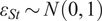
$ {\varepsilon}_{St}\sim N\left(0,1\right) $
 and
$ {\tau}_A $
and
$ {\tau}_A $
 is the tax rate with
$ {\tau}_A=0 $
is the tax rate with
$ {\tau}_A=0 $
 as the baseline value.
The annuitization ratio defines what happens to the retirement saving balance upon death. In non-annuitized plans, savings go to the heirs of the account holder at death, after subtracting income tax since contributions are made before tax. In valuation terms, this is equivalent to the case where the product issuer after the death of the account holder continues to make the scheduled payments but to the heirs of the deceased. In contrast, lifelong annuities provide regular payments to the account holder until death, and the heirs receive nothing from the annuity provider, who effectively distributes the remaining savings to surviving customers’ accounts. I also consider “partial annuities” with an annuitization ratio
$ I\in \left[0,1\right] $
 so that the annuity provider retains the fraction
$ I $
so that the annuity provider retains the fraction
$ I $
 of savings upon death in retirement, while the remainder is paid to the heirs. For a large group of individuals of age
$ t\ge {t}_R $
of savings upon death in retirement, while the remainder is paid to the heirs. For a large group of individuals of age
$ t\ge {t}_R $
 with similar survival probabilities and account balances, the balance of each member surviving until age
$ t+1 $
with similar survival probabilities and account balances, the balance of each member surviving until age
$ t+1 $
 can be added a fraction
$ {d}_t=I\left(1-{p}_t\right)/{p}_t $
can be added a fraction
$ {d}_t=I\left(1-{p}_t\right)/{p}_t $
 of the balance at the end of year
$ t $
of the balance at the end of year
$ t $
 due to transfers from deceased customers.
Scheduled payouts are made from age
$ {t}_F $
 to
$ {t}_L $
to
$ {t}_L $
 , and I focus on the case
$ {t}_R={t}_F $
, and I focus on the case
$ {t}_R={t}_F $
 and
$ {t}_L={t}_M $
and
$ {t}_L={t}_M $
 and assume contributions to the account are made only before time
$ {t}_F $
and assume contributions to the account are made only before time
$ {t}_F $
 .Footnote
8 The scheduled payout policy is captured by an age-dependent function
$ {m}_t $
.Footnote
8 The scheduled payout policy is captured by an age-dependent function
$ {m}_t $
 stating the fraction of the retirement saving balance paid out at age
$ t $
stating the fraction of the retirement saving balance paid out at age
$ t $
 . If
$ {A}_t $
. If
$ {A}_t $
 is the opening balance in year
$ t $
is the opening balance in year
$ t $
 , the scheduled monetary payout in year
$ t $
, the scheduled monetary payout in year
$ t $
 is
$ {m}_t{A}_t $
is
$ {m}_t{A}_t $
 . Next year’s balance is

I set
$ {m}_{t_L}=1 $
 so the remaining balance
$ {A}_{t_L} $
so the remaining balance
$ {A}_{t_L} $
 is paid out at age
$ {t}_L $
is paid out at age
$ {t}_L $
 .
.
The payout profiles I consider are controlled by a parameter
$ x $
 , the so-called excess assumed interest rate (AIR), together with the expected investment returns and mortality risk. The payout rates are specified recursively as

Since
$ {e}^{-x}={\mathrm{E}}_t\left[{m}_{t+1}{A}_{t+1}\right]/\left({m}_t{A}_t\right) $
 , the excess AIR
$ x $
, the excess AIR
$ x $
 reflects the drop in expected payouts per year. For
$ x=0 $
reflects the drop in expected payouts per year. For
$ x=0 $
 , expected payouts are flat, which is a common feature of pension plans (for payments in real terms, constant payments mean CPI-adjusted payments). Details can be found in the Supplementary Material.
As a simple example, assume 0 returns and taxes. A person turning 67 then needs un-annuitized savings of $340,000 to ensure $10,000 of consumption per year in case the person should live until the end of year 100 but only fully annuitized savings of $185,405 to ensure $10,000 per year until the end of life given the mortality rates of the U.S. population.
The costs associated with a retirement saving plan are also crucial. My model assumes that the individual can privately invest without any trading or participation costs in a risk-free asset and in a stock index, so the modeled returns are really net of any such costs (e.g., the low cost on index ETFs). I assume that managing a retirement saving plan is not more costly than managing private, non-retirement funds. Any administrative fees charged by the plan provider (maybe $100–200 per year) are assumed to be similar to the costs (time consumption, etc.) of handling private investments.
Annuities are often considered expensive. Mitchell et al. (Reference Mitchell, Poterba, Warshawsky and Brown1999) report that for a 65-year-old annuitant the money’s worth ratio of U.S. lifelong annuities is around 85%, depending on the annuitant’s gender and the discount rate used, and assuming population mortality rates. Hence, I assume a 15% cost on an annuity (
$ I=1 $
 ) relative to a personal account (
$ I=0 $
) relative to a personal account (
$ I=0 $
 ). Other studies report similar costs with variations across countries and products (Kaschützke and Maurer (Reference Kaschützke, Maurer, Mitchell, Piggott and Takayama2011)). These costs may stem from assessing and managing how the lifetime uncertainty of annuity buyers differs from that of the population and relates to adverse selection issues, in which individuals with a longer-than-average life expectancy benefit from a contract based on the population’s life expectancy. A 15% charge roughly covers the extra payments if the annuitant’s life expectancy at retirement is
$ \left(1/0.85\right)-1\approx 17.6\% $
). Other studies report similar costs with variations across countries and products (Kaschützke and Maurer (Reference Kaschützke, Maurer, Mitchell, Piggott and Takayama2011)). These costs may stem from assessing and managing how the lifetime uncertainty of annuity buyers differs from that of the population and relates to adverse selection issues, in which individuals with a longer-than-average life expectancy benefit from a contract based on the population’s life expectancy. A 15% charge roughly covers the extra payments if the annuitant’s life expectancy at retirement is
$ \left(1/0.85\right)-1\approx 17.6\% $
 longer than for the entire population. In the 2019 U.S. life table, an individual turning 67 can expect to live another 18 years, so for an annuity holder the same life expectancy can be up to 21.2 years without eliminating profits for the annuity issuer. For partial annuities with
$ 0<I<1 $
longer than for the entire population. In the 2019 U.S. life table, an individual turning 67 can expect to live another 18 years, so for an annuity holder the same life expectancy can be up to 21.2 years without eliminating profits for the annuity issuer. For partial annuities with
$ 0<I<1 $
 , the cost is assumed proportional to
$ I $
, the cost is assumed proportional to
$ I $
 , so the money’s worth ratio is

where a dollar contributed to retirement savings increases the account balance by
$ W(I) $
 dollars.
B. Plans with Constant Expected Payouts Throughout Retirement
Table 1 shows payouts for plans with constant expected payouts (
$ x=0 $
 ) combining the four investment strategies specified previously and three values (0, 0.5, and 1) of the annuitization ratio
$ I $
) combining the four investment strategies specified previously and three values (0, 0.5, and 1) of the annuitization ratio
$ I $
 . The individual is assumed in Panel A to spend $100 on each product when retiring at age 67 and in Panel B to contribute an amount
$ a $
. The individual is assumed in Panel A to spend $100 on each product when retiring at age 67 and in Panel B to contribute an amount
$ a $
 at the beginning of every year from age 25 to 66. To facilitate comparisons across the panels, I fix
$ a=100\hskip0.1em {e}^{-r}\left(1-{e}^r\right)/\left(1-{e}^{r\left({T}_R-25\right)}\right)\approx 1.9603 $
at the beginning of every year from age 25 to 66. To facilitate comparisons across the panels, I fix
$ a=100\hskip0.1em {e}^{-r}\left(1-{e}^r\right)/\left(1-{e}^{r\left({T}_R-25\right)}\right)\approx 1.9603 $
 so that a risk-free investment strategy with
$ I=0 $
so that a risk-free investment strategy with
$ I=0 $
 generates a wealth of $100 at retirement. In both cases, the product issuer subtracts costs so that only the fraction
$ W(I) $
generates a wealth of $100 at retirement. In both cases, the product issuer subtracts costs so that only the fraction
$ W(I) $
 of the contribution is invested to generate future payouts to the customer. For each case, the table shows the expected annual payout and the 10th and 90th percentiles in the distribution of possible payouts at ages 70, 80, 90, and 99. For plans involving stock investments, all numbers are based on 100,000 simulations of the annual stock returns.

TABLE 1 Long description
Panel A presents payouts for a one-time investment of 100 dollars at age 67. Panel B shows payouts for constant contributions from ages 25 to 66. Each panel is organized by stock weight (0, 0.5, 1, T D F) and annuitization ratio (0, 0.5, 1). For each plan, columns display expected annual payout, 10th percentile payout at ages 70, 80, 90, and 99, and 90th percentile payout at the same ages. In Panel A, for stock weight 0 and annuitization ratio 0, all payouts are 3.45 dollars. Increasing annuitization ratio raises expected payouts, with values up to 7.30 dollars for stock weight 1 and annuitization ratio 1. Percentile columns show greater spread as stock weight and annuitization ratio increase, with 90th percentile payouts reaching 15.37 dollars at age 99 for stock weight 1 and annuitization ratio 1. T D F rows reflect glide path strategies, with expected payouts ranging from 4.26 to 5.88 dollars. Panel B, for constant contributions, shows similar structure. For stock weight 0 and annuitization ratio 0, payouts remain at 3.45 dollars. Higher stock weight and annuitization ratio yield larger expected payouts, up to 24.05 dollars for stock weight 1 and annuitization ratio 1. The 90th percentile at age 99 reaches 53.85 dollars for this plan. T D F rows in Panel B show expected payouts from 8.77 to 14.16 dollars, with 90th percentile values up to 25.14 dollars. Across both panels, increasing stock weight and annuitization ratio consistently raise expected and percentile payouts, with greater variability at higher values.
Table 1 illustrates two points. First, stock investments lead to notably higher expected payouts, in particular when savings are gradually built up as in Panel B. Focus on non-annuitized plans. The risk-free investment generates an annual payout of $3.45, whereas one fully invested in stocks leads to an expected annual payout of $5.97 if initiated at retirement and $16.75 if built up over working life. The higher expected payout comes with a high upside potential and some downside risk. With the target-date fund (TDF), the expected annual payout is more modest but both the upside potential and the downside risk are, of course, lower than with a full stock investment. With gradual savings, the annual payout with the TDF strategy has an expectation of $8.77 and thus 154% larger than with the risk-free strategy, and the TDF payout beats the risk-free payout at any age with a probability of more than 90%, cf. the 10th percentiles ranging from $4.12 to $3.62, so the downside risk is limited compared to the sizeable upside potential. Individuals might also not be as concerned about the significant downside payout risk of stock-heavy plans at high ages (the 10th percentiles decrease in age), since they have only a small chance of surviving that long.
Second, the payouts increase significantly with the annuitization ratio
$ I $
 despite larger costs. With
$ I=0 $
despite larger costs. With
$ I=0 $
 the payments must be stretched out until the maximum age, whereas with
$ I=1 $
the payments must be stretched out until the maximum age, whereas with
$ I=1 $
 the payments are only due until death. With a $100 investment at retirement, the (expected) annual payout with
$ I=1 $
the payments are only due until death. With a $100 investment at retirement, the (expected) annual payout with
$ I=1 $
 is 48% larger than for
$ I=0 $
is 48% larger than for
$ I=0 $
 ($5.09 compared to $3.45) when
$ w=0 $
($5.09 compared to $3.45) when
$ w=0 $
 and 22% larger ($7.30 compared to $5.97) when
$ w=1 $
and 22% larger ($7.30 compared to $5.97) when
$ w=1 $
 . With the gradual saving strategy, the (expected) annual payout is 70% larger with
$ I=1 $
. With the gradual saving strategy, the (expected) annual payout is 70% larger with
$ I=1 $
 than
$ I=0 $
than
$ I=0 $
 when
$ w=0 $
when
$ w=0 $
 and 44% larger when
$ w=1 $
and 44% larger when
$ w=1 $
 , and the 10th and 90th percentiles increase similarly.
The downside of a higher
$ I $
 is a lower bequest upon death. Figure 1 shows how the expected account value of selected plans varies with age. The value of plans being built up from age 25 (light-colored curves) increases until retirement, and then savings decumulate in retirement—also for plans initiated at retirement (dark curves)—to 0 at the maximum age. The solid curves represent non-annuitized plans and depict the pre-tax account value bequeathed in case of death at each age. The dashed curves represent the fully annuitized plans. The orange curves are for plans with
$ w=1 $
is a lower bequest upon death. Figure 1 shows how the expected account value of selected plans varies with age. The value of plans being built up from age 25 (light-colored curves) increases until retirement, and then savings decumulate in retirement—also for plans initiated at retirement (dark curves)—to 0 at the maximum age. The solid curves represent non-annuitized plans and depict the pre-tax account value bequeathed in case of death at each age. The dashed curves represent the fully annuitized plans. The orange curves are for plans with
$ w=1 $
 (index-linked) and the blue curves for plans with
$ w=0 $
(index-linked) and the blue curves for plans with
$ w=0 $
 (risk-free). The orange curves with savings from age 25 show that the account value is lower with
$ I=1 $
(risk-free). The orange curves with savings from age 25 show that the account value is lower with
$ I=1 $
 than
$ I=0 $
than
$ I=0 $
 , except for a few final years. At first, this is due to costs being subtracted. Later, transfers from deceased plan holders are added to the account when
$ I=1 $
, except for a few final years. At first, this is due to costs being subtracted. Later, transfers from deceased plan holders are added to the account when
$ I=1 $
 , reducing the distance between the curves toward 0 at retirement. In retirement, the value of the annuitized plan first declines more steeply due to larger payouts, but, when the mortality rate picks up, increasing transfers from deceased portfolio holders bring the two curves closer. An individual with a fully annuitized instead of a non-annuitized version of the risk-free plan receives an extra annual payout of
$ \$5.09-\$3.45=\$1.64 $
, reducing the distance between the curves toward 0 at retirement. In retirement, the value of the annuitized plan first declines more steeply due to larger payouts, but, when the mortality rate picks up, increasing transfers from deceased portfolio holders bring the two curves closer. An individual with a fully annuitized instead of a non-annuitized version of the risk-free plan receives an extra annual payout of
$ \$5.09-\$3.45=\$1.64 $
 every year until death but, on the other hand, at death the heirs do not receive the pre-tax annuity value which is $65.72 at age 80 and $36.14 at age 90. Obviously, an individual’s choice of plan depends on preferences for bequests versus consumption and on life expectancy.
In Figure 1, the individual’s age is depicted along the horizontal axis. The blue lines show the value of a risk-free plan at the beginning of each year, and the orange-red lines the expected value of an index-linked plan. The solid lines represent personal products
$ \left(I=0\right) $
 and the dashed lines lifelong annuities (
$ I=1 $
and the dashed lines lifelong annuities (
$ I=1 $
 ). The dark-colored lines are for plans initiated at retirement with a $100 investment, whereas the light-colored lines are for a plan with gradual savings of $1.9063 every year from age 25 to retirement at age 67 (indicated by (G) in the legend). Additional information can be found in the main text.

FIGURE 1 Long description
The horizontal axis shows age from 25 to 105. The vertical axis shows account value from 0 to 300. Eight lines are plotted: blue for risk-free, orange-red for index-linked. Solid lines represent personal products, dashed lines lifelong annuities. Dark lines show a 100 dollar lump sum at retirement, light lines show gradual savings of 1.9063 dollars yearly from age 25 to 67, labeled with (G). For both risk-free and index-linked, values rise steadily until age 67, peaking for index-linked plans, then decline. Index-linked plans (orange-red) reach higher peaks than risk-free (blue). Lifelong annuities (dashed) decline more gradually after retirement than personal products (solid). Gradual savings lines (light) are always below lump sum lines (dark) but follow similar shapes. The legend at the top specifies line color and style for each scenario: w equals 0 or 1, l equals 0 or 1, and (G) for gradual savings.
C. Plans with Other Payout Schedules
Table 2 provides examples of plans with age-dependent expected payouts controlled by the excess AIR
$ x $
 . With
$ x<0 $
. With
$ x<0 $
 and thus payouts increasing with age, more returns are made on savings, which leads to larger average payouts. A negative
$ x $
and thus payouts increasing with age, more returns are made on savings, which leads to larger average payouts. A negative
$ x $
 generates a more steeply increasing payout when
$ I=1 $
generates a more steeply increasing payout when
$ I=1 $
 than when
$ I=0 $
than when
$ I=0 $
 . This follows from the mortality risk being increasing in age and the fact that payouts with
$ I=1 $
. This follows from the mortality risk being increasing in age and the fact that payouts with
$ I=1 $
 are conditional on survival. Hence, large conditional payouts late in life can be promised without reducing earlier payouts much. For example, with
$ w=0 $
are conditional on survival. Hence, large conditional payouts late in life can be promised without reducing earlier payouts much. For example, with
$ w=0 $
 and
$ x=-8\% $
and
$ x=-8\% $
 , expected payouts increase from
$ \$0.94 $
, expected payouts increase from
$ \$0.94 $
 at age 70 to $9.57 at age 99 when
$ I=0 $
at age 70 to $9.57 at age 99 when
$ I=0 $
 but from $2.37 to $24.15 when
$ I=1 $
but from $2.37 to $24.15 when
$ I=1 $
 . For
$ x>0 $
. For
$ x>0 $
 and thus declining payouts, the difference in payments between
$ I=0 $
and thus declining payouts, the difference in payments between
$ I=0 $
 and
$ I=1 $
and
$ I=1 $
 is smaller since the scheduled payments are low when mortality risk is high. The table also shows the 10th percentiles of annual payouts for the index-linked plans (
$ w=1 $
is smaller since the scheduled payments are low when mortality risk is high. The table also shows the 10th percentiles of annual payouts for the index-linked plans (
$ w=1 $
 ). With a positive
$ x $
). With a positive
$ x $
 , not only are expected payouts declining with age, there is also a large probability of ending up with very low payouts when living long. Note that plans with
$ w=1 $
, not only are expected payouts declining with age, there is also a large probability of ending up with very low payouts when living long. Note that plans with
$ w=1 $
 and
$ x=-4\% $
and
$ x=-4\% $
 have 10th percentiles being roughly flat through retirement together with increasing expected payouts.
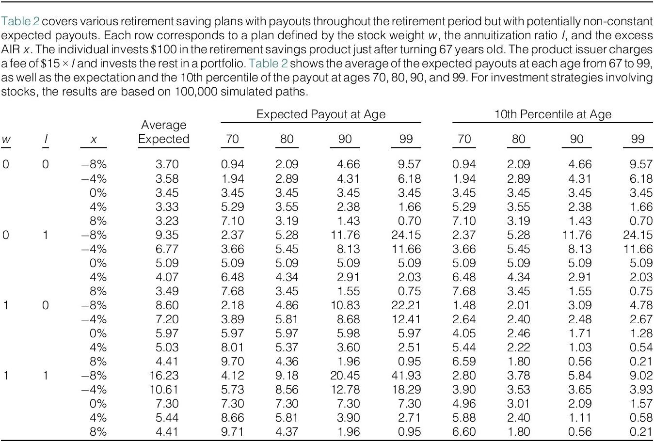
TABLE 2 Long description
Starting from the top row, the table lists combinations of stock weight w, annuitization ratio I, and excess AIR x. For each combination, columns show average payout, expected payout at ages 70, 80, 90, 99, and 10th percentile at those ages. For w equals 0 and I equals 0, x ranges from minus 8 percent to plus 8 percent. Average payouts decrease as x increases, from 3.70 at minus 8 percent to 3.23 at plus 8 percent. Expected payouts at age 70 rise from 0.94 to 7.10, while at age 99 they fall from 9.57 to 0.70. The 10th percentile follows similar trends. For w equals 0 and I equals 1, average payouts are higher, ranging from 9.35 to 3.49 as x increases. Expected payouts at age 70 rise from 2.37 to 7.68, and at age 99 fall from 24.15 to 0.75. The 10th percentile at age 70 rises from 2.37 to 7.68, and at age 99 falls from 24.15 to 0.75. For w equals 1 and I equals 0, average payouts range from 8.60 to 4.41 as x increases. Expected payouts at age 70 rise from 2.18 to 9.71, and at age 99 fall from 22.21 to 0.21. The 10th percentile at age 70 rises from 1.48 to 6.60, and at age 99 falls from 4.78 to 0.21. For w equals 1 and I equals 1, average payouts range from 16.23 to 4.41 as x increases. Expected payouts at age 70 rise from 4.12 to 9.71, and at age 99 fall from 41.93 to 0.21. The 10th percentile at age 70 rises from 2.80 to 6.60, and at age 99 falls from 9.02 to 0.21. Across all rows, higher annuitization ratios and stock weights generally increase average and expected payouts at younger ages, but decrease payouts at older ages and lower percentiles as excess AIR increases.
D. Required Minimum Distributions
U.S. legislation stipulates required minimum distributions (RMDs) that individuals must withdraw from their retirement accounts each year starting at age 73 (as of 2023); any required amounts not withdrawn are subject to a 50% tax. The RMD in dollar terms for a given age
$ t\ge 73 $
 is the account balance at the end of the previous year divided by a so-called distribution period associated with that age, which is published by the Internal Revenue Service (IRS), related to the remaining life expectancy, and thus decreasing with age. This regulation effectively defines a lower bound
$ {\underline{m}}_t $
is the account balance at the end of the previous year divided by a so-called distribution period associated with that age, which is published by the Internal Revenue Service (IRS), related to the remaining life expectancy, and thus decreasing with age. This regulation effectively defines a lower bound
$ {\underline{m}}_t $
 on the payout rate
$ {m}_t $
on the payout rate
$ {m}_t $
 introduced previously with
$ {\underline{m}}_t $
introduced previously with
$ {\underline{m}}_t $
 being equal to the reciprocal of the distribution period for that age.Footnote
9
being equal to the reciprocal of the distribution period for that age.Footnote
9
All plans considered previously with a 0 excess AIR satisfy the RMD bound, no matter what the annuitization ratio is. The solid curves in Figure 2 show the payout rates for some of these plans (on a log scale), and they are all above the dashed black curve that represents the lower bound. Graph A considers target-date fund strategies (IP4). The upper solid curve is for full annuitization (
$ I=1 $
 ), the lower for no annuitization (
$ I=0 $
), the lower for no annuitization (
$ I=0 $
 ). As discussed earlier, payout rates are increasing in
$ I $
). As discussed earlier, payout rates are increasing in
$ I $
 . Graph B considers the strategies with either 0%, 50%, or 100% in stocks (IP1–3) and no annuitization. As payout rates are increasing in expected returns, the upper solid curve is for the most aggressive strategy. The curve for the least aggressive strategy barely meets the requirement; for example, the payout rate at age 73 is 4.07% while the minimum is 3.77%.
Figure 2 shows payout rates
$ {m}_t $
 as a function of age
$ t $
as a function of age
$ t $
 for different retirement saving plans. Graph A considers plans where investments follow the target-date fund strategy with solid curves representing plans with an excess AIR of
$ x=0 $
for different retirement saving plans. Graph A considers plans where investments follow the target-date fund strategy with solid curves representing plans with an excess AIR of
$ x=0 $
 and dotted curves plans with
$ x=-10\% $
and dotted curves plans with
$ x=-10\% $
 ; the orange curves are for plans with full annuitization (
$ I=1 $
; the orange curves are for plans with full annuitization (
$ I=1 $
 ) and the gray curves for plans with no annuitization (
$ I=0 $
) and the gray curves for plans with no annuitization (
$ I=0 $
 ). The black-dashed curve depicts the required minimum distribution. Graph B considers non-annuitized plans with a constant stock weight of either
$ w=0 $
). The black-dashed curve depicts the required minimum distribution. Graph B considers non-annuitized plans with a constant stock weight of either
$ w=0 $
 (orange curves),
$ w=0.5 $
(orange curves),
$ w=0.5 $
 (gray curves), or
$ w=1 $
(gray curves), or
$ w=1 $
 (blue curves); the solid curves are for plans with an excess AIR of
$ x=0 $
(blue curves); the solid curves are for plans with an excess AIR of
$ x=0 $
 and the dotted curves for plans with
$ x=-10\% $
and the dotted curves for plans with
$ x=-10\% $
 . Note that the vertical axes have a logarithmic scale.
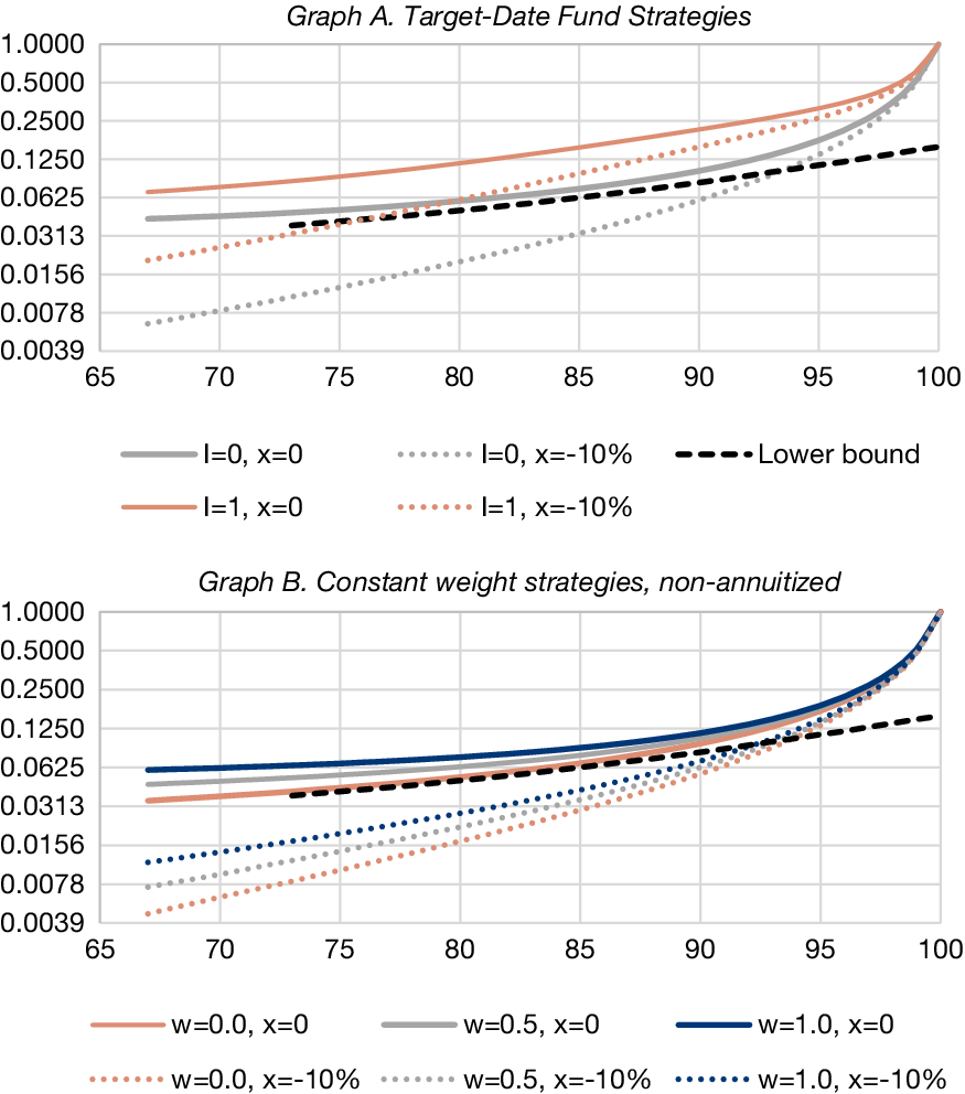
FIGURE 2 Long description
The top panel, labeled Graph A. Target-Date Fund Strategies, plots payout rate m sub t on the y-axis (logarithmic scale from 0.0039 to 0.5) against age t on the x-axis (65 to 100). Four curves are shown: solid gray for I equals 0, x equals 0; dotted gray for I equals 0, x equals minus 10 percent; solid orange for I equals 1, x equals 0; dotted orange for I equals 1, x equals minus 10 percent. A black dashed line labeled Lower bound runs between the solid and dotted curves. All curves rise with age, with the highest payout at age 100 for I equals 1, x equals 0, and the lowest for I equals 0, x equals minus 10 percent. The bottom panel, labeled Graph B. Constant weight strategies, non-annuitized, uses the same axes. Six curves are shown: solid orange for w equals 0, x equals 0; dotted orange for w equals 0, x equals minus 10 percent; solid gray for w equals 0.5, x equals 0; dotted gray for w equals 0.5, x equals minus 10 percent; solid blue for w equals 1, x equals 0; dotted blue for w equals 1, x equals minus 10 percent. The black dashed Lower bound is also present. All curves increase with age, with the highest payout at age 100 for w equals 1, x equals 0, and the lowest for w equals 0, x equals minus 10 percent. Legends below each panel match curve color and style to strategy parameters.
Payout rates are increasing in the excess AIR. Consequently, plans with a sufficiently negative AIR—and thus very steeply increasing expected payments—violate the lower bound. The dotted curves in Figure 2 represent strategies with an excess AIR of
$ -10\% $
 , and they all fall below the lower bound over some age interval starting at age 73. In particular, for plans with low expected returns and no annuitization, the excess AIR can only be mildly negative (i.e., expected payouts can only be slowly increasing with age). Plans with high expected returns and full annuitization can have more steeply increasing expected payouts. For the TDF strategy, the lowest acceptable excess AIR is
$ -8\% $
, and they all fall below the lower bound over some age interval starting at age 73. In particular, for plans with low expected returns and no annuitization, the excess AIR can only be mildly negative (i.e., expected payouts can only be slowly increasing with age). Plans with high expected returns and full annuitization can have more steeply increasing expected payouts. For the TDF strategy, the lowest acceptable excess AIR is
$ -8\% $
 with full annuitization and increases to
$ 0\% $
with full annuitization and increases to
$ 0\% $
 with no annuitization. For the all-in-stocks strategy, the lowest acceptable excess AIR is
$ -10\% $
with no annuitization. For the all-in-stocks strategy, the lowest acceptable excess AIR is
$ -10\% $
 with full annuitization and increases to
$ -4\% $
with full annuitization and increases to
$ -4\% $
 with no annuitization.Footnote
10
with no annuitization.Footnote
10
III. A Life-Cycle Model
I set up a life-cycle model to evaluate different retirement saving plans and to find the optimal retirement saving decisions of an individual consumer investor. The model adapts the mandatory pension saving model of Larsen and Munk (Reference Larsen and Munk2023), and I refer to their paper for details and for additional motivation of the baseline parameter values listed in Table 3. I model income and wealth in real terms (current dollars), and all returns are also in real terms. The model has annual time steps and represents the decision problem of an individual who has just turned
$ {t}_1=25 $
 years old, retires when turning
$ {t}_R=67 $
years old, retires when turning
$ {t}_R=67 $
 years old, and may live on until the end of her year
$ {t}_M=100 $
years old, and may live on until the end of her year
$ {t}_M=100 $
 . As earlier,
$ {p}_t $
. As earlier,
$ {p}_t $
 denotes the probability of being alive at age
$ t+1 $
denotes the probability of being alive at age
$ t+1 $
 conditional on being alive at age
$ t $
conditional on being alive at age
$ t $
 .
.
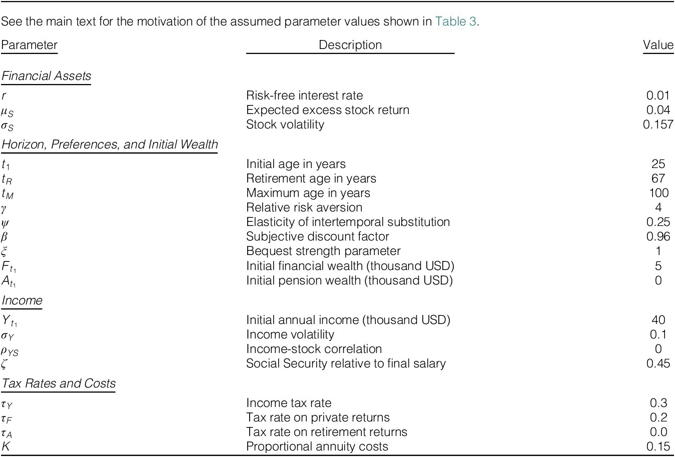
TABLE 3 Long description
From the top, the table is divided into four sections. The first section, Financial assets, lists r as risk-free interest rate 0.01, mu sub S as expected excess stock return 0.04, and sigma sub S as stock volatility 0.157. The next section, Horizon, preferences, and initial wealth, includes t sub 1 as initial age 25, t sub R as retirement age 67, t sub M as maximum age 100, gamma as relative risk aversion 4, psi as elasticity of intertemporal substitution 0.25, beta as subjective discount factor 0.96, xi as bequest strength parameter 1, F sub t sub 1 as initial financial wealth 5 thousand U S D, and A sub t sub 1 as initial pension wealth 0. The third section, Income, lists Y sub t sub 1 as initial annual income 40 thousand U S D, sigma sub Y as income volatility 0.1, rho sub Y S as income-stock correlation 0, and zeta as Social Security relative to final salary 0.45. The final section, Tax rates and costs, includes tau sub Y as income tax rate 0.3, tau sub F as tax rate on private returns 0.2, tau sub A as tax rate on retirement returns 0.0, and K as proportional annuity costs 0.15. All values are presented in the rightmost column.
A. Income, Social Security, and Medical Costs
The individual receives pre-tax income
$ {Y}_t $
 at the beginning of year
$ t $
at the beginning of year
$ t $
 from labor, a state pension, or other sources. The income dynamics are

where

with
$ {\varepsilon}_{Yt}\sim N\left(0,1\right) $
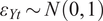 and independent over time. The income starts at
$ {Y}_{t_1}=\$\mathrm{40,000} $
and independent over time. The income starts at
$ {Y}_{t_1}=\$\mathrm{40,000} $
 , has a volatility of
$ {\sigma}_Y=10\% $
, has a volatility of
$ {\sigma}_Y=10\% $
 , and the expected growth rate
$ {\mu}_{Yt} $
, and the expected growth rate
$ {\mu}_{Yt} $
 follows a third-order polynomial with coefficients determined so that expected income peaks at age 55 at a value 50% above initial income and then drops 10% until retirement. The income is assumed uncorrelated with the stock index.Footnote
11
$ \zeta =0.45 $
follows a third-order polynomial with coefficients determined so that expected income peaks at age 55 at a value 50% above initial income and then drops 10% until retirement. The income is assumed uncorrelated with the stock index.Footnote
11
$ \zeta =0.45 $
 is the ratio of the annual state pension to pre-retirement income and leads to an expected after-tax annual state pension of $17,328.
Out-of-pocket medical costs are a major concern for U.S. retirees and can significantly impact saving and risk taking (De Nardi, French, and Jones (Reference De Nardi, French and Jones2010)). I let
$ {\phi}_t,{\Phi}_t\in \left\{0,1\right\} $
 indicate whether an uninsured health shock with a small cost
$ h=3\% $
indicate whether an uninsured health shock with a small cost
$ h=3\% $
 (e.g., for prescription medicine), respectively, large cost
$ H=85\% $
(e.g., for prescription medicine), respectively, large cost
$ H=85\% $
 (e.g., for nursing home spending), occurs at age
$ t $
(e.g., for nursing home spending), occurs at age
$ t $
 . The small-shock probability is the constant
$ q=\mathrm{Prob}\left({\phi}_t=1\right)=18\% $
. The small-shock probability is the constant
$ q=\mathrm{Prob}\left({\phi}_t=1\right)=18\% $
 , whereas the large-shock probability
$ {Q}_t=\mathrm{Prob}\left({\Phi}_t=1\right)=\min \left\{0.03\times \frac{t-{t}_R}{t_M-{t}_R}+{\left(\frac{{\left(t-{t}_R-15\right)}^{+}}{t_M-{t}_R-15}\right)}^2,\mathrm{0.5}\right\} $
, whereas the large-shock probability
$ {Q}_t=\mathrm{Prob}\left({\Phi}_t=1\right)=\min \left\{0.03\times \frac{t-{t}_R}{t_M-{t}_R}+{\left(\frac{{\left(t-{t}_R-15\right)}^{+}}{t_M-{t}_R-15}\right)}^2,\mathrm{0.5}\right\} $
 grows linearly until 15 years into retirement, where it accelerates until reaching 50%. The medical costs are assumed to be tax deductible so
$ h $
grows linearly until 15 years into retirement, where it accelerates until reaching 50%. The medical costs are assumed to be tax deductible so
$ h $
 and
$ H $
and
$ H $
 reflect the percentage reduction in income both before and after tax. Model simulations show that medical costs are expected to be 3.4%, 11.1%, 23.8%, and 77.9% of Social Security pay at ages 72, 79, 86, and 93, broadly in line with Koijen, van Nieuwerburgh, and Yogo (Reference Koijen, van Nieuwerburgh and Yogo2016) and De Nardi, French, Jones, and McCauley (Reference De Nardi, French, Jones and McCauley2016). For simplicity, life expectancy is assumed unchanged after a medical shock, and the shocks are assumed permanent (transitory shocks have little impact anyway).
B. Investments and Wealth Dynamics
Both the pension fund and the individual can invest in a risk-free asset and a stock index. As in Section II, the risk-free log return is
$ r $
 per year, and the index has normally distributed log returns over any period
$ dt $
per year, and the index has normally distributed log returns over any period
$ dt $
 with expectation
$ \left(r+{\mu}_S-\frac{1}{2}{\sigma}_S^2\right)\hskip0.1em dt $
with expectation
$ \left(r+{\mu}_S-\frac{1}{2}{\sigma}_S^2\right)\hskip0.1em dt $
 and standard deviation
$ {\sigma}_S\hskip0.1em \sqrt{dt} $
and standard deviation
$ {\sigma}_S\hskip0.1em \sqrt{dt} $
 and with returns being independent across time.Footnote
12
and with returns being independent across time.Footnote
12
I let
$ {F}_t $
 denote the individual’s private wealth (outside the retirement account) and assume
$ {F}_{t_1}=\$\mathrm{5,000} $
denote the individual’s private wealth (outside the retirement account) and assume
$ {F}_{t_1}=\$\mathrm{5,000} $
 .Footnote
13 At the beginning of each year, the individual i) receives income and (in retirement) scheduled or self-selected payouts from her retirement saving account, ii) makes a scheduled or self-selected contribution to the retirement account, iii) pays income taxes, and iv) decides how much to consume and how to invest the remaining private wealth over the year. The contribution to the retirement account is a fraction
$ {\alpha}_t\in \left[0,\overline{\alpha}\right) $
.Footnote
13 At the beginning of each year, the individual i) receives income and (in retirement) scheduled or self-selected payouts from her retirement saving account, ii) makes a scheduled or self-selected contribution to the retirement account, iii) pays income taxes, and iv) decides how much to consume and how to invest the remaining private wealth over the year. The contribution to the retirement account is a fraction
$ {\alpha}_t\in \left[0,\overline{\alpha}\right) $
 of pre-tax income with
$ {\alpha}_t=0 $
of pre-tax income with
$ {\alpha}_t=0 $
 for
$ t\ge {T}_R $
for
$ t\ge {T}_R $
 . Annual contributions to a 401(k) plan in the United States are currently capped at $23,000 (2024-level, annually revised). If the cap is constant in real terms, it also applies close to retirement when income is expected to be up to around 50% higher than the initial $40,000, and this is when high contribution rates are attractive in some cases. Hence, I set the upper bound to
$ \overline{\alpha}=0.4 $
. Annual contributions to a 401(k) plan in the United States are currently capped at $23,000 (2024-level, annually revised). If the cap is constant in real terms, it also applies close to retirement when income is expected to be up to around 50% higher than the initial $40,000, and this is when high contribution rates are attractive in some cases. Hence, I set the upper bound to
$ \overline{\alpha}=0.4 $
 .
.
The year
$ t $
 payout from the retirement account is
$ {m}_t{A}_t $
payout from the retirement account is
$ {m}_t{A}_t $
 , where
$ {A}_t $
, where
$ {A}_t $
 is the account balance entering year
$ t $
is the account balance entering year
$ t $
 . I require
$ {m}_t=0 $
. I require
$ {m}_t=0 $
 for
$ t<{T}_R $
for
$ t<{T}_R $
 . For plans involving any annuitization (
$ I>0 $
. For plans involving any annuitization (
$ I>0 $
 ), the individual is part of a joint risk-sharing arrangement with other individuals and must stick to the scheduled payouts
$ {m}_t{A}_t $
), the individual is part of a joint risk-sharing arrangement with other individuals and must stick to the scheduled payouts
$ {m}_t{A}_t $
 described in Section II, and only plans satisfying the RMD are allowed. For a non-annuitized plan (
$ I=0 $
described in Section II, and only plans satisfying the RMD are allowed. For a non-annuitized plan (
$ I=0 $
 ), the individual’s retirement savings are separate from other individuals so the individual can choose the payout ratio
$ {m}_t $
), the individual’s retirement savings are separate from other individuals so the individual can choose the payout ratio
$ {m}_t $
 each year under the RMD constraint
$ {m}_t\ge {\underline{m}}_t $
each year under the RMD constraint
$ {m}_t\ge {\underline{m}}_t $
 . The balance
$ {A}_t $
. The balance
$ {A}_t $
 of the retirement account starts at
$ {A}_{t_1}=0 $
of the retirement account starts at
$ {A}_{t_1}=0 $
 . Adding contributions with annuity-linked costs to (2), the retirement account balance at the beginning of year
$ t+1 $
. Adding contributions with annuity-linked costs to (2), the retirement account balance at the beginning of year
$ t+1 $
 , provided the individual survives year
$ t $
, provided the individual survives year
$ t $
 , is
, is

The income after contributions to—or payouts from—the retirement account is subject to a proportional tax rate of
$ {\tau}_Y=30\% $
 . The disposable private wealth in year
$ t $
. The disposable private wealth in year
$ t $
 is
is

of which the individual consumes a fraction
$ {c}_t\in \left(0,1\right] $
 . The remainder is invested and, with
$ {R}_{Ft} $
. The remainder is invested and, with
$ {R}_{Ft} $
 denoting the gross after-tax return, next year’s private wealth becomes

I assume the private portfolio is continuously rebalanced to keep a constant fraction
$ {\pi}_t $
 of wealth in the stock index throughout year
$ t $
of wealth in the stock index throughout year
$ t $
 . All private returns—realized or not—are taxed year-end at a rate of
$ {\tau}_F=20\% $
. All private returns—realized or not—are taxed year-end at a rate of
$ {\tau}_F=20\% $
 . Similarly to Eq. (1), the after-tax gross return is then

C. Preferences and Decisions
The retirement saving plans I consider are characterized by
$ {t}_F,{t}_L,I,x $
 , and
$ w=\left({w}_t\right) $
, and
$ w=\left({w}_t\right) $
 . For a plan with self-selected contributions, the individual chooses
$ {c}_t $
. For a plan with self-selected contributions, the individual chooses
$ {c}_t $
 ,
$ {\pi}_t $
,
$ {\pi}_t $
 , and
$ {\alpha}_t $
, and
$ {\alpha}_t $
 for
$ t={t}_1,{t}_1+1,\dots, {t}_M $
for
$ t={t}_1,{t}_1+1,\dots, {t}_M $
 (and
$ {m}_t $
(and
$ {m}_t $
 if
$ I=0 $
if
$ I=0 $
 ) to maximize lifetime utility. I assume Epstein-Zin utility with indirect utility
$ {J}_t $
) to maximize lifetime utility. I assume Epstein-Zin utility with indirect utility
$ {J}_t $
 satisfying the recursion

where appropriate bounds are imposed on the controls
$ {c}_t,{\pi}_t,{\alpha}_t $
 , and where

is the certainty equivalent of next period’s utility which is
$ {J}_{t+1} $
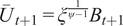
 if surviving and the bequest utility
$ {\overline{U}}_{t+1}={\xi}^{\frac{1}{\psi -1}}{B}_{t+1} $
if surviving and the bequest utility
$ {\overline{U}}_{t+1}={\xi}^{\frac{1}{\psi -1}}{B}_{t+1} $
 if not. The bequest if dying at the end of year
$ t $
if not. The bequest if dying at the end of year
$ t $
 is the sum of the private wealth and the fraction
$ 1-I $
is the sum of the private wealth and the fraction
$ 1-I $
 of after-tax retirement wealth,

Should the individual reach the maximum age, the pension account has already been paid out, so
$ {B}_{t_M+1}={F}_{t_M+1} $
 . Without access to a retirement saving plan, the choice variable
$ \alpha $
. Without access to a retirement saving plan, the choice variable
$ \alpha $
 and the state variable
$ A $
and the state variable
$ A $
 are identical to 0.
Base case preferences are characterized by the relative risk aversion (RRA)
$ \gamma =4 $
 , the elasticity of intertemporal substitution (EIS)
$ \psi =0.25 $
, the elasticity of intertemporal substitution (EIS)
$ \psi =0.25 $
 , the subjective discount factor
$ \beta =0.96 $
, the subjective discount factor
$ \beta =0.96 $
 , and the strength of the bequest motive
$ \xi =1 $
, and the strength of the bequest motive
$ \xi =1 $
 , but I also consider alternative values.Footnote
14
, but I also consider alternative values.Footnote
14
Given my setup, the indirect utility is a function
$ {J}_t\left({F}_t,{Y}_t,{A}_t\right) $
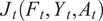 of age, private wealth, income, and retirement savings. The dimension of the state space can be reduced by 1 by exploiting a homogeneity property (see the Supplementary Material):

where

Here
$ {a}_t $
 is bounded by 0 and 1, whereas
$ {y}_t $
is bounded by 0 and 1, whereas
$ {y}_t $
 is bounded from below by 0 but unbounded from above. Both
$ {A}_t $
is bounded from below by 0 but unbounded from above. Both
$ {A}_t $
 and
$ {F}_t $
and
$ {F}_t $
 depend on the optimal controls so that
$ {y}_t $
depend on the optimal controls so that
$ {y}_t $
 typically starts out very high as annual income tends to be large relative to financial wealth for young individuals. As wealth accumulates over life,
$ {y}_t $
typically starts out very high as annual income tends to be large relative to financial wealth for young individuals. As wealth accumulates over life,
$ {y}_t $
 typically drops considerably approaching retirement and then jumps down at retirement after which it varies again due to medical costs and wealth decumulation.Footnote
15 I solve for
$ G $
typically drops considerably approaching retirement and then jumps down at retirement after which it varies again due to medical costs and wealth decumulation.Footnote
15 I solve for
$ G $
 and optimal decisions by backward dynamic programming on a grid. I simulate 10,000 paths forward and report averages at each age to indicate an expected life-cycle pattern. Of course, without access to a retirement saving plan the variable
$ a $
and optimal decisions by backward dynamic programming on a grid. I simulate 10,000 paths forward and report averages at each age to indicate an expected life-cycle pattern. Of course, without access to a retirement saving plan the variable
$ a $
 is identical to 0 and the dimension is thus reduced further.
D. Utility Gain Measure
Let
$ {J}_{t_1}\left(F,Y;\mathrm{P}\right) $
 denote the initial (age 25) indirect utility when the individual follows the retirement saving plan
$ \mathrm{P} $
denote the initial (age 25) indirect utility when the individual follows the retirement saving plan
$ \mathrm{P} $
 defined by a specific combination of
$ {t}_F,{t}_L,I,x $
defined by a specific combination of
$ {t}_F,{t}_L,I,x $
 , and
$ w=\left({w}_t\right) $
, and
$ w=\left({w}_t\right) $
 . The initial retirement account value is 0, so
$ A $
. The initial retirement account value is 0, so
$ A $
 is dropped from the notation. As a common benchmark, I compare with the indirect lifetime utility
$ {J}_{t_1}\left(F,Y;\mathrm{no}\right) $
is dropped from the notation. As a common benchmark, I compare with the indirect lifetime utility
$ {J}_{t_1}\left(F,Y;\mathrm{no}\right) $
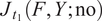 when the individual does not have access to any retirement saving plan. If the individual is not forced to save in the retirement saving product, she is at least as well off with access to such a product as without. I quantify the utility gain to the individual of having plan
$ \mathrm{P} $
when the individual does not have access to any retirement saving plan. If the individual is not forced to save in the retirement saving product, she is at least as well off with access to such a product as without. I quantify the utility gain to the individual of having plan
$ \mathrm{P} $
 by the fraction
$ \lambda $
by the fraction
$ \lambda $
 of additional lifetime labor income and initial wealth that the individual without any plan would need to receive to obtain the same lifetime utility as with access to the plan. With the additional income and wealth, the indirect utility without retirement saving products is
$ {J}_{t_1}\left(\left[1+\lambda \right]F,\left[1+\lambda \right]Y;\mathrm{no}\right)=\left(1+\lambda \right){J}_{t_1}\left(F,Y;\mathrm{no}\right). $
of additional lifetime labor income and initial wealth that the individual without any plan would need to receive to obtain the same lifetime utility as with access to the plan. With the additional income and wealth, the indirect utility without retirement saving products is
$ {J}_{t_1}\left(\left[1+\lambda \right]F,\left[1+\lambda \right]Y;\mathrm{no}\right)=\left(1+\lambda \right){J}_{t_1}\left(F,Y;\mathrm{no}\right). $
 Equating this with
$ {J}_{t_1}\left(F,Y;\mathrm{P}\right) $
Equating this with
$ {J}_{t_1}\left(F,Y;\mathrm{P}\right) $
 , I find

Following Larsen and Munk (Reference Larsen and Munk2023), I transform the utility gain into a dollar amount by multiplying
$ \lambda $
 by the sum of the initial financial wealth and the present value (PV) of lifetime after-tax income (from labor and Social Security less medical expenses). Since the income is not spanned by traded assets, there is no unique way to fix the discount rate for future expected income. I apply a discount rate of 3.55%, the sum of the risk-free rate 1% and a premium of
$ 4\%\times 10\%/15.7\% $
by the sum of the initial financial wealth and the present value (PV) of lifetime after-tax income (from labor and Social Security less medical expenses). Since the income is not spanned by traded assets, there is no unique way to fix the discount rate for future expected income. I apply a discount rate of 3.55%, the sum of the risk-free rate 1% and a premium of
$ 4\%\times 10\%/15.7\% $
 calculated as a volatility-scaling of the equity premium. The PV of lifetime income is then $859,242 and adding the financial wealth of $5,000, a utility gain
$ \lambda $
calculated as a volatility-scaling of the equity premium. The PV of lifetime income is then $859,242 and adding the financial wealth of $5,000, a utility gain
$ \lambda $
 of 1% corresponds to $8,642.
IV. Optimal Decisions and Plans: Base Case Preferences
This section focuses on individuals with base case preference parameters. First, I illustrate optimal decisions with and without access to pension plans. Next, I show how the utility and outcomes of the individual are affected by a range of basic plans (i.e., plans with either no or full annuitization and with flat expected payouts). Finally, I add plan flexibility in the form of partial annuitization and non-flat expected payouts.
A. Optimal Decisions With and Without a Pension Plan
As shown in the next subsection, the optimal basic pension plan features full annuitization, a TDF investment strategy, and self-selected contributions. Figure 3 illustrates the optimal controls with and without this pension plan. The controls are shown at three different age levels and always as functions of the ratio
$ y $
 of income to total wealth; note that the relevant range of
$ y $
of income to total wealth; note that the relevant range of
$ y $
 and thus the horizontal axis in these graphs change with age. With access to a pension plan, the controls also depend on the ratio
$ a $
and thus the horizontal axis in these graphs change with age. With access to a pension plan, the controls also depend on the ratio
$ a $
 of pension wealth to total wealth, and I show the controls for
$ a=0.3 $
of pension wealth to total wealth, and I show the controls for
$ a=0.3 $
 (labeled “low”) and
$ a=0.6 $
(labeled “low”) and
$ a=0.6 $
 (“high”).
Figure 3 shows, at different age levels, how optimal controls vary with the income–wealth ratio
$ y $
 . Graph A shows
$ c $
. Graph A shows
$ c $
 (i.e., the optimal consumption as a fraction of disposable wealth). Graph B shows
$ \pi $
(i.e., the optimal consumption as a fraction of disposable wealth). Graph B shows
$ \pi $
 (i.e., the fraction of private wealth invested in stocks). Graph C shows the contribution rate
$ \alpha $
(i.e., the fraction of private wealth invested in stocks). Graph C shows the contribution rate
$ \alpha $
 ( i.e., the fraction of income saved in the pension account). The solid gray curves are for the case without a pension plan. With a pension plan, the optimal controls also depend on
$ a $
( i.e., the fraction of income saved in the pension account). The solid gray curves are for the case without a pension plan. With a pension plan, the optimal controls also depend on
$ a $
 , the fraction of pension wealth to total wealth. Here, the dashed orange curves are for
$ a=0.3 $
, the fraction of pension wealth to total wealth. Here, the dashed orange curves are for
$ a=0.3 $
 and the dotted green lines are for
$ a=0.6 $
and the dotted green lines are for
$ a=0.6 $
 . The baseline parameter values from Table 3 are assumed. The pension plan applied is the optimal basic pension plan with full annuitization and the target-date investment strategy.

FIGURE 3 Long description
Top row shows consumption over disposable wealth versus y for ages 30, 60, and 90. All panels compare no plan, plan low a, and plan high a. At age 30, all lines rise quickly then plateau, with plan high a highest. At age 60 and 90, plan high a remains above others, with flatter curves. Middle row shows stock weight versus y for the same ages. At age 30, all lines are flat near 1 except fund, which is lower. At age 60, plan high a and plan low a rise sharply then plateau, while no plan and fund remain flat and lower. At age 90, plan high a and plan low a are higher and slightly variable, fund and no plan are lower and flatter. Bottom row shows contribution rate versus y for ages 30, 45, and 60. At age 30, plan low a and plan high a start near zero, spike, then stabilize. At age 45, plan low a rises then falls, plan high a is lower and flatter. At age 60, both plan low a and plan high a quickly rise and plateau near 0.4. Legends and axes are consistent across panels.
Graph A of Figure 3 show that the consumption–wealth ratio
$ c $
 is increasing in
$ y $
is increasing in
$ y $
 with or without the pension plan and in
$ a $
with or without the pension plan and in
$ a $
 with the plan. The consumption–wealth ratio is large for a young individual with little wealth, decreases until retirement where total wealth peaks, after which it often increases as wealth is decumulated. The consumption–wealth ratio is larger with access to the pension plan (dotted curves) than without (solid curves).
Graph B of Figure 3 show the plan’s stock weight (flat blue line) and the optimal private stock weight
$ \pi $
 with (dotted curves) or without the plan (solid dark curves). Due to the bond-like human capital, the private stock weight is at the maximum 100% for the young individual and tends to decrease with age when the income–wealth ratio drops, as is known from standard life-cycle models (e.g., Cocco et al. (Reference Cocco, Gomes and Maenhout2005)). At age 60, the stock weight is still 100% if the income–wealth ratio is high but below 100% if the income–wealth ratio is low. At age 90, the human capital is small (only the PV of Social Security in the remaining years) and has little impact on the stock weight which is therefore lower and approaching the no-income Merton weight of
$ {\mu}_S/\left({\gamma \sigma}_S^2\right)\approx 0.406 $
with (dotted curves) or without the plan (solid dark curves). Due to the bond-like human capital, the private stock weight is at the maximum 100% for the young individual and tends to decrease with age when the income–wealth ratio drops, as is known from standard life-cycle models (e.g., Cocco et al. (Reference Cocco, Gomes and Maenhout2005)). At age 60, the stock weight is still 100% if the income–wealth ratio is high but below 100% if the income–wealth ratio is low. At age 90, the human capital is small (only the PV of Social Security in the remaining years) and has little impact on the stock weight which is therefore lower and approaching the no-income Merton weight of
$ {\mu}_S/\left({\gamma \sigma}_S^2\right)\approx 0.406 $
 . An individual with a pension plan adjusts the private stock weight so that the stock weight in her total portfolio comes close to what is optimal in the absence of a pension plan. At age 90, the plan’s 30% stock weight is too low relative to the benchmark individual’s optimal total stock weight, so she invests a larger fraction of private wealth in stocks, and more so if
$ a $
. An individual with a pension plan adjusts the private stock weight so that the stock weight in her total portfolio comes close to what is optimal in the absence of a pension plan. At age 90, the plan’s 30% stock weight is too low relative to the benchmark individual’s optimal total stock weight, so she invests a larger fraction of private wealth in stocks, and more so if
$ a $
 is high so that a lot of wealth is tied up in the pension plan. Due to the more lenient return taxation, the individual prefers more stocks in the retirement account than in the private account.
Graph C of Figure 3 show the optimal contribution rate
$ \alpha $
 to the preferred pension plan at ages 30, 45, and 60. The optimal contribution rate
$ \alpha $
to the preferred pension plan at ages 30, 45, and 60. The optimal contribution rate
$ \alpha $
 is low—in most cases 0—at age 30. A young individual who has preferences for consumption smoothing and expects a significant income growth does not want to save much in an illiquid pension account but builds up a small private buffer for “rainy days.” At age 45, the incentives for pension savings are bigger: much of the income growth is already realized, a private buffer has been built, and the retirement period is getting closer. The optimal contribution rate is lower if
$ a $
is low—in most cases 0—at age 30. A young individual who has preferences for consumption smoothing and expects a significant income growth does not want to save much in an illiquid pension account but builds up a small private buffer for “rainy days.” At age 45, the incentives for pension savings are bigger: much of the income growth is already realized, a private buffer has been built, and the retirement period is getting closer. The optimal contribution rate is lower if
$ a $
 is large (i.e., a relatively large pension wealth has already been accumulated). The contribution rate is hump-shaped in
$ y $
is large (i.e., a relatively large pension wealth has already been accumulated). The contribution rate is hump-shaped in
$ y $
 , so if income is either low or high relative to total wealth, a smaller fraction of income is contributed to the pension account compared to the case with a medium income–wealth ratio. At age 60, the individual contributes in many cases the maximum 40% of income. At this age, pension savings are preferred to private savings because of the more lenient return taxation, and the individual is not concerned with the illiquidity of the pension savings as retirement is near and pension payouts are thus starting soon.
While the optimal control diagrams in Figure 3 are informative, they must be coupled with the probabilities of ending up in different values of
$ y $
 and
$ a $
and
$ a $
 at each age level to see typical life-cycle patterns. Hence, I simulate 10,000 possible lifetime paths. Along each path, I draw random numbers to represent the annual shocks to labor income, stock prices, and health costs. Starting from the stated initial values and using the optimal controls derived with my numerical optimization approach, this generates life-cycle paths of income, consumption, portfolio weights, contribution rates, private wealth, pension wealth, and so forth. The age-specific averages across the 10,000 paths indicate expected life-cycle patterns.
Graph A of Figure 4 shows that expected consumption (solid curves) has the hump-shaped life-cycle pattern seen in the data (Thurow (Reference Thurow1969), Gourinchas and Parker (Reference Gourinchas and Parker2002)). The dotted-blue curve shows expected income (including Social Security) after tax and health costs. Expected consumption is larger at every age when the individual has access to the pension plan. The dashed curves indicate the 5th percentile of consumption which is also larger with the pension plan than without, so the plan reduces the risk of low consumption at any age and mostly so in retirement.
Figure 4 shows expected consumption, saving rates, private stock weight, and wealth as a function of age, both without a pension plan (solid dark curves) and with a pension plan characterized by a TDF investment strategy, full annuitization, and flat expected payouts. Graph A shows consumption with a plan (orange) and expected income after tax and medical expenses (dotted blue), as well as the 5th percentiles of consumption at each age without (dashed gray) and with (dashed orange) the pension plan. For the case with access to the plan, the graphs with saving rates, stock weight, and wealth show both the private component (orange) and the pension component (yellow). Graph D also depicts total wealth with a pension plan (green). Parameter values are taken from Table 3. The income and plan wealth shown are after income tax.

FIGURE 4 Long description
Top-left panel: X-axis is age from 25 to 100, Y-axis is consumption in k U S D from 0 to 45. Four lines: solid gray for mean consumption without plan, solid brown for mean with plan, dashed gray for 5th percentile without plan, dashed brown for 5th percentile with plan, and dotted blue for income. Both mean consumption lines rise to a peak near age 65, then decline; the plan line stays above the no-plan line, especially after retirement. The 5th percentile lines are lower, with the plan line consistently above the no-plan line. Income drops sharply at retirement age. Top-right panel: X-axis is age from 25 to 65, Y-axis is saving rates from -0.2 to 0.4. Three lines: solid gray for private saving without plan, solid brown for private saving with plan, and yellow for pension contribution. Private saving rates are positive and stable without a plan, but decline and turn negative with a plan after age 55. Pension contribution rises with age, peaking near retirement. Bottom-left panel: X-axis is age from 25 to 100, Y-axis is stock weight from 0 to 1.2. Three lines: solid gray for private stock weight without plan, solid brown for private stock weight with plan, yellow for pension plan stock weight. Private stock weight is high and stable without a plan, but declines after age 65 with a plan. Pension plan stock weight declines steadily with age. Bottom-right panel: X-axis is age from 25 to 100, Y-axis is wealth in k U S D from 0 to 600. Four lines: solid gray for total wealth without plan, solid brown for private wealth with plan, yellow for pension plan wealth, green for total wealth with plan. All wealth lines rise to a peak near age 65, then decline. Total wealth with plan (green) is lower than without plan (gray), but the pension plan (yellow) adds to private wealth (brown) to form the total.
Graph B of Figure 4 illustrates that, without a pension plan (dark curve), the fraction of income saved starts at around 15%, is almost flat until age 45, and then declines significantly and turns negative at age 60. With a pension plan, the individual saves both privately (orange curve) and via the pension plan (yellow curve). In the early years, the individual prefers private savings to build up a liquid wealth buffer, but pension contributions increase from about 5% at age 30 to 10% around age 50 and then steeply to 30% in the final years before retirement, where wealth is moved from the private account to the pension account.Footnote 16
Graph C shows that, without the pension plan (dark curve), the individual invests all savings in stocks until around age 55, where the stock weight starts to decline and ends up around 50%. The yellow kinked line depicts the glide path strategy of the pension plan which this individual finds too conservative, so the private stock weight (orange curve) is kept at 100% longer and subsequently kept larger than in the case without a plan.
Graph D displays the typical tent-shaped wealth pattern. With the pension plan, most of the wealth is accumulated in the plan (yellow curve) with an expected after-tax value of $333,000 at retirement. Private wealth (orange curve) peaks at age 57 at $122,000, is reduced to $50,000 toward retirement (financing high contributions), and then grows to $73,000 in the late 1980s, mainly due to the risk of large medical expenses. Total expected wealth is lower with a plan (green curve) than without (dark curve), for example, $371,000 versus $491,000 at age 65. The plan’s annuitization insures the individual against “outliving her wealth” so lower savings are needed which facilitates higher consumption throughout life.
B. Basic Pension Plans
The top row of Table 4 refers to the benchmark case with no pension plan, where the optimal decisions lead to an expected ratio of private wealth to after-tax income of 1.9 at age 35, 6.1 at age 50, and 14.3 at age 65. In retirement, the ratio is calculated using the Social Security benefits as income (without subtracting medical costs), so the ratio increases at retirement where income drops. Subsequently, the ratio declines when wealth is decumulated to finance consumption expenditures exceeding Social Security but, as indicated by the wealth–income ratio of 21.1 at age 85, the decumulation is slow since the individual faces the risk of substantial medical costs as well as the risk of living long in which case wealth must cover consumption for many years.
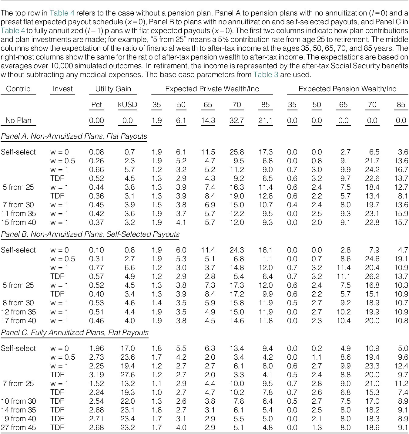
TABLE 4 Long description
Panel A covers non-annuitized plans with flat payouts. The top row shows no plan, with utility gain at 0.00 percent and expected private wealth-to-income ratios rising from 1.9 at age 35 to 32.7 at age 70, then 21.1 at age 85. Pension wealth-to-income remains zero. Subsequent rows detail self-select and fixed contribution methods, each with investment types (w equals 0, 0.5, 1, T D F). Utility gain increases with higher w, peaking at 0.66 percent for self-select w equals 1. Expected private wealth-to-income ratios generally increase with age and contribution, while pension wealth-to-income ratios rise notably at ages 65 and above for higher w and T D F. Panel B presents non-annuitized plans with self-selected payouts. Utility gain ranges from 0.10 percent to 0.77 percent for self-select, and up to 0.53 percent for fixed contributions. Private wealth-to-income ratios show similar age progression, with pension wealth-to-income ratios increasing at older ages, especially for higher w and T D F. Panel C displays fully annuitized plans with flat payouts. Utility gain is highest, reaching 3.19 percent for self-select T D F. Private wealth-to-income ratios are lower than in Panels A and B, but pension wealth-to-income ratios are substantially higher, peaking at 27.6 at age 50 for self-select T D F. Across all panels, utility gain and pension wealth-to-income ratios are maximized in fully annuitized plans with T D F investments and higher contribution rates.
Table 4 shows utility gains, relative to the no-plan case, and private and pension wealth relative to income for a range of basic pension plans following one of the investment strategies IP1–4. When choosing each year the contribution to a non-annuitized plan with a preset flat payout schedule, the individual prefers a plan with full stock investments, cf. Panel A of Table 4. This generates a utility gain of 0.66% or $5,700 in PV terms. The accumulated pension wealth relative to income is expected to be 0.7 at age 35, 3.0 at age 50, and 9.9 at age 65, jumps at retirement, and then declines as payouts are made. With this plan, less private wealth is accumulated. At age 65, the aggregate expected wealth–income ratio is 15.1 (sum of 5.2 and 9.9), compared to 14.3 in the no-plan case. The utility gain is lower for the other investment strategies, for example, 0.52% with a TDF strategy. By definition, utility gains are lower with a predetermined contribution schedule instead of self-selected contributions. As explained previously, the individual dislikes plans with large contributions in early adulthood, and the best fixed contribution rate is 5% when contributions are made from age 25, 7% from age 30, 11% from age 35, and 15% from age 40. For these plans, the gain reduction relative to the plan with self-selected contributions is modest as the individual can undo much of the unwanted pension savings by adjusting private savings.
Also the additional utility gain from selecting the payout ratio each year instead of following a preset schedule is modest, cf. Panel B of Table 4. For example, with self-selected contributions and the all-stocks strategy, the utility gain is 0.77% with self-selected payouts compared to 0.66% with flat payouts. The modest difference is partly due to the RMD lower bound that limits the individual’s flexibility regarding payout ratios. With self-selected payouts, the pension savings are accessible throughout retirement, so the individual can substitute private savings by pension savings and thereby reduce capital gain taxes.
Panel C of Table 4 shows that utility gains are substantially larger with the fully annuitized plans than the non-annuitized plans, despite the assumed 15% cost of annuities. Non-annuitized plans benefit individuals only through lower capital gains taxes, whereas fully annuitized plans also allow individuals to share lifetime risks and thus provide insurance against living long. On the other hand, with annuitized plans, individuals must stick to a predetermined payout schedule which, in this section, is required to deliver flat expected payouts. With fully annuitized plans, the baseline individual prefers that pension savings are invested following the TDF strategy. With self-selected contributions, this leads to a utility gain of 3.19% (or $27,600) instead of 0.77% [0.66%] for the non-annuitized plan with self-selected [flat] payouts. While the expected pension wealth–income ratio is similar in the two cases, the private wealth–income ratio is considerably lower with the fully annuitized plan than with the similar non-annuitized plan with flat payouts, for example, 2.0 instead of 4.3 at age 65 with self-selected contributions and the TDF strategy.
Among fully annuitized plans with a constant contribution rate, a 7% contribution is optimal if contributions must be made from age 25, but the individual is better off with a larger contribution rate if contributions start later, for example, a plan with 19% contributions from age 40 leads to a utility gain of 2.71%, not far from the 3.19% gain with self-selected contributions. If well designed, plans leaving few choices to individuals (and thus being less exposed to behavioral mistakes) can still lead to substantial utility gains.
C. Flexible Pension Plans
Table 5 explores how much the base-case individual appreciates payout flexibility in the form of partial annuitization (
$ I $
 less than 1) and non-flat expected payouts (
$ x $
less than 1) and non-flat expected payouts (
$ x $
 different from 0). For all plans considered, pension savings are invested according to the TDF strategy, which is the optimal strategy of the base-case individual for most plans, including those generating the largest utility gains. For tractability, I consider only
$ I $
different from 0). For all plans considered, pension savings are invested according to the TDF strategy, which is the optimal strategy of the base-case individual for most plans, including those generating the largest utility gains. For tractability, I consider only
$ I $
 in multiples of
$ 0.1 $
in multiples of
$ 0.1 $
 and
$ x $
and
$ x $
 in multiples of 2% and, given the RMD lower payout bound,
$ -8\% $
in multiples of 2% and, given the RMD lower payout bound,
$ -8\% $
 is the lowest admissible value for the fully annuitized plan with a TDF strategy. Among plans with self-selected contributions, Panel A shows that when maintaining flat expected payouts, the optimal annuitization ratio is 0.9 which leads to an increase in the utility gain of only 0.07 percentage points compared to full annuitization. Panel B shows that when maintaining full annuitization, a plan with an excess AIR of
$ -4\% $
is the lowest admissible value for the fully annuitized plan with a TDF strategy. Among plans with self-selected contributions, Panel A shows that when maintaining flat expected payouts, the optimal annuitization ratio is 0.9 which leads to an increase in the utility gain of only 0.07 percentage points compared to full annuitization. Panel B shows that when maintaining full annuitization, a plan with an excess AIR of
$ -4\% $
 (i.e., expected payouts increasing by about 4% each year) adds 0.33 percentage points to the utility gain compared to flat payouts. Panel C shows that when varying both, the optimal annuitization ratio is still 0.9 and the excess AIR still
$ -4\% $
(i.e., expected payouts increasing by about 4% each year) adds 0.33 percentage points to the utility gain compared to flat payouts. Panel C shows that when varying both, the optimal annuitization ratio is still 0.9 and the excess AIR still
$ -4\% $
 with a combined incremental utility gain of 0.38 percentage points or around $3,300 in PV terms.
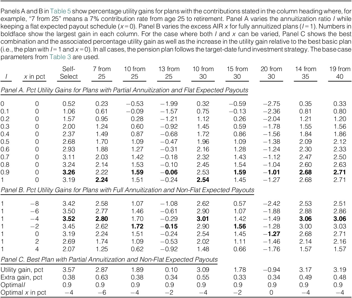
TABLE 5 Long description
Panel A presents percentage utility gains for plans with partial annuitization and flat expected payouts. The leftmost column lists annuitization ratio I from 0 to 1 in increments of 0.1, with x fixed at 0. The top row shows contribution scenarios: Self-Select, 7 from 25, 10 from 25, 13 from 25, 10 from 30, 15 from 30, 20 from 30, 14 from 35, and 19 from 40. Each cell contains the utility gain in percent, with boldface indicating the highest gain per column. For example, at I equal to 0.9, Self-Select yields 3.26, 10 from 25 yields 1.59, 13 from 25 yields negative 0.06, 15 from 30 yields 1.59, 20 from 30 yields negative 1.01, 14 from 35 yields 2.68, and 19 from 40 yields 2.71. Panel B shows utility gains for fully annuitized plans (I equal to 1) with non-flat expected payouts, where x varies from negative 8 to 4. Columns are the same as Panel A. Highest values per column are bolded, such as 3.52 for Self-Select at x equal to negative 4, 2.80 for 7 from 25, 3.01 for 10 from 30, 3.06 for 14 from 35 and 19 from 40. Panel C summarizes the best plan for each contribution scenario, listing utility gain, extra gain, optimal I, and optimal x. For example, Self-Select achieves a utility gain of 3.57 percent, extra gain of 0.38 percent, optimal I of 0.9, and optimal x of negative 4. All panels use base case parameters and a target-date fund investment strategy.
The other columns of Table 5 show similar results for plans with a fixed contribution rate from a certain age. The lower the contribution rate and the later the starting age, the less valuable is partial annuitization and the more valuable is a more steeply increasing payout schedule. When both
$ I $
 and
$ x $
and
$ x $
 are flexible, an annuitization ratio
$ I $
are flexible, an annuitization ratio
$ I $
 of 0.9 is optimal for all plans, and most plans are best with a negative excess AIR
$ x $
of 0.9 is optimal for all plans, and most plans are best with a negative excess AIR
$ x $
 and thus increasing expected payouts through retirement. The additional utility gain is between 0.33 and 0.63 percentage points ($2,800–$5,500 in PV terms) compared to the basic version of the plan.
In my main specification, the individual selects the payout parameters
$ I $
 and
$ x $
and
$ x $
 when initiating the pension plan at age 25. The Supplementary Material considers the alternative specification where
$ I $
when initiating the pension plan at age 25. The Supplementary Material considers the alternative specification where
$ I $
 and
$ x $
and
$ x $
 are chosen at retirement depending on the individual’s pre-tax income
$ Y $
are chosen at retirement depending on the individual’s pre-tax income
$ Y $
 , private wealth
$ F $
, private wealth
$ F $
 , and pension wealth
$ A $
, and pension wealth
$ A $
 entering retirement. Across a range of combinations of
$ Y $
entering retirement. Across a range of combinations of
$ Y $
 ,
$ F $
,
$ F $
 , and
$ A $
, and
$ A $
 , the optimal annuitization ratio is 0.9 for the base-case individual and thus identical to the optimal choice at age 25 for all the contribution schemes covered by Table 5. When pension wealth is relatively small and private wealth large, the optimal excess AIR
$ x $
, the optimal annuitization ratio is 0.9 for the base-case individual and thus identical to the optimal choice at age 25 for all the contribution schemes covered by Table 5. When pension wealth is relatively small and private wealth large, the optimal excess AIR
$ x $
 at retirement is
$ -8\% $
at retirement is
$ -8\% $
 so that the small pension wealth is decumulated slowly at the beginning of retirement. When pension wealth is relatively large and private wealth small, the optimal
$ x $
so that the small pension wealth is decumulated slowly at the beginning of retirement. When pension wealth is relatively large and private wealth small, the optimal
$ x $
 at retirement is
$ -4\% $
at retirement is
$ -4\% $
 or even
$ -2\% $
or even
$ -2\% $
 so that the large pension wealth is decumulated more rapidly, although still with increasing payouts through time. These findings are consistent with Table 5 where a more negative
$ x $
so that the large pension wealth is decumulated more rapidly, although still with increasing payouts through time. These findings are consistent with Table 5 where a more negative
$ x $
 is chosen at age 25 for plans with lower contributions. Letting the individual choose these parameters at retirement invalidates the homogeneity property (12) before retirement and thus drastically increases computational complexity (see the Supplementary Material), so I do not consider optimal pre-retirement behavior and initial utility gains for this specification. However, the results indicate some additional utility gains from delaying the choice of excess AIR until retirement.
V. Preferred Plans of Different Individuals
This section presents results for individuals with different characteristics. Compared to the baseline case, I consider the effects of changing one parameter at a time: an RRA
$ \gamma $
 of 2 or 6 (instead of 4), an EIS
$ \psi $
of 2 or 6 (instead of 4), an EIS
$ \psi $
 of 0.1 or 0.5 (instead of 0.25), a bequest weight
$ \xi $
of 0.1 or 0.5 (instead of 0.25), a bequest weight
$ \xi $
 of 0.2 or 5 (instead of 1), a subjective discount factor
$ \beta $
of 0.2 or 5 (instead of 1), a subjective discount factor
$ \beta $
 of 0.93 or 0.99 (instead of 0.96), and an initial pre-tax annual income
$ {Y}_{t_1} $
of 0.93 or 0.99 (instead of 0.96), and an initial pre-tax annual income
$ {Y}_{t_1} $
 of $30,000 or $50,000 (instead of $40,000).Footnote
17
of $30,000 or $50,000 (instead of $40,000).Footnote
17
Panel A of Table 6 shows the best basic plans for the different individuals, that is, plans with i) full annuitization (
$ I=1 $
 ) and preset flat expected payouts (
$ x=0 $
) and preset flat expected payouts (
$ x=0 $
 ) or ii) no annuitization with self-selected payouts respecting the RMD lower bound. The utility gains range from 0.81% to 5.07% or from $6,996 to $43,811 in PV terms. The RRA 2 individual has the smallest gain and, as the only individual considered, prefers a non-annuitized plan that invests all savings in stocks. The utility gain is completely due to the tax advantage for this individual, who is willing to keep a low liquid wealth and thus build up significant retirement savings with high expected and untaxed returns. All other individuals prefer a fully annuitized plan, despite the 15% cost and Social Security benefits, with savings invested according to the TDF strategy. The largest gains are obtained by the individuals with a high discount factor or high RRA, who are most concerned with ensuring a decent consumption level if they should live long. The individual with a high bequest incentive builds up more liquid wealth (which can be bequeathed) than pension wealth, whereas the other individuals are willing to tie up most of their wealth in the pension account. For all individuals, a big part of their pension wealth at retirement stems from large contributions in the years just before retirement, as was illustrated for the base case preferences in Figure 4. Especially for individuals with a high RRA, a low bequest weight, or a high discount factor, the gains are much larger for the fully annuitized plans than for the corresponding non-annuitized plans. For example, with RRA 6, the utility gain is only 0.84% for the non-annuitized plan with preset flat expected payouts compared to 4.97% with the fully annuitized plan.
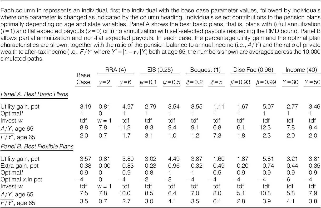
TABLE 6 Long description
Panel A, titled Best Basic Plans, presents columns for the base case and parameter variations: R R A (gamma equals 2 and gamma equals 6), E I S (psi equals 0.1 and psi equals 0.5), Bequest (xi equals 0.2 and xi equals 5), Discount Factor (beta equals 0.93 and beta equals 0.99), and Income (Y equals 30 and Y equals 50). Rows show utility gain in percent (base: 3.19, gamma equals 2: 0.81, gamma equals 6: 4.97, psi equals 0.1: 2.79, psi equals 0.5: 3.54, xi equals 0.2: 3.55, xi equals 5: 1.11, beta equals 0.93: 1.67, beta equals 0.99: 5.07, Y equals 30: 2.77, Y equals 50: 3.46), optimal I (base: 1, gamma equals 2: 0, all others: 1), investment w (base: t d f, gamma equals 2: w equals 1, all others: t d f), average A all over Y at age 65 (base: 8.8, gamma equals 2: 7.8, gamma equals 6: 11.2, psi equals 0.1: 8.3, psi equals 0.5: 9.4, xi equals 0.2: 9.1, xi equals 5: 6.8, beta equals 0.93: 6.1, beta equals 0.99: 12.3, Y equals 30: 7.8, Y equals 50: 9.4), and average F all over Y prime at age 65 (base: 2.0, gamma equals 2: 0.7, gamma equals 6: 1.7, psi equals 0.1: 3.1, psi equals 0.5: 1.0, xi equals 0.2: 1.2, xi equals 5: 7.3, beta equals 0.93: 1.8, beta equals 0.99: 2.3, Y equals 30: 2.0, Y equals 50: 2.0). Panel B, titled Best Flexible Plans, follows the same column structure. Rows show utility gain in percent (base: 3.57, gamma equals 2: 0.81, gamma equals 6: 5.80, psi equals 0.1: 3.02, psi equals 0.5: 4.49, xi equals 0.2: 3.87, xi equals 5: 1.60, beta equals 0.93: 1.87, beta equals 0.99: 5.81, Y equals 30: 3.21, Y equals 50: 3.81), extra gain in percent (base: 0.38, gamma equals 2: 0.00, gamma equals 6: 0.83, psi equals 0.1: 0.23, psi equals 0.5: 0.96, xi equals 0.2: 0.32, xi equals 5: 0.49, beta equals 0.93: 0.20, beta equals 0.99: 0.74, Y equals 30: 0.44, Y equals 50: 0.35), optimal I (base: 0.9, gamma equals 2: 0, gamma equals 6: 0.9, psi equals 0.1: 0.8, psi equals 0.5: 1, xi equals 0.2: 1, xi equals 5: 0.5, beta equals 0.93: 0.9, beta equals 0.99: 0.9, Y equals 30: 0.9, Y equals 50: 0.9), optimal x in percent (base: minus 4, gamma equals 2: 0, gamma equals 6: minus 4, psi equals 0.1: minus 2, psi equals 0.5: minus 8, xi equals 0.2: minus 4, xi equals 5: minus 4, beta equals 0.93: minus 4, beta equals 0.99: minus 4, Y equals 30: minus 6, Y equals 50: minus 4), investment w (base: t d f, gamma equals 2: w equals 1, all others: t d f), average A all over Y at age 65 (base: 7.5, gamma equals 2: 7.8, gamma equals 6: 10.0, psi equals 0.1: 8.5, psi equals 0.5: 6.4, xi equals 0.2: 7.0, xi equals 5: 8.0, beta equals 0.93: 5.1, beta equals 0.99: 10.8, Y equals 30: 5.8, Y equals 50: 7.9), and average F all over Y prime at age 65 (base: 3.5, gamma equals 2: 0.7, gamma equals 6: 2.7, psi equals 0.1: 3.0, psi equals 0.5: 4.1, xi equals 0.2: 3.5, xi equals 5: 6.1, beta equals 0.93: 2.8, beta equals 0.99: 3.9, Y equals 30: 4.1, Y equals 50: 3.8).
Panel B of Table 6 allows partial annuitization and non-flat payouts. While the RRA 2 individual still prefers the non-annuitized plan, the other individuals appreciate the extra flexibility with an additional utility gain of up to 0.96 percentage points or $8,257. Most individuals prefer an annuitization ratio around 0.9, but, as expected, the individual with a high bequest incentive selects a lower value. Most individuals choose a plan with expected payouts increasing around 4% each year. The flexibility in scheduled payouts affect the saving patterns of the individuals. The base-case individual accumulates less wealth in the pension plan and more private wealth when having access to the preferred flexible plan than the preferred basic plan: at age 65, the ratio of pension wealth to annual income is 7.5 instead of 8.8 and the ratio of private wealth to annual after-tax income is 3.5 instead of 2.0. A few individuals change their saving behavior in the opposite direction. For example, for the individual with high-bequest weight, the age-65 ratio of pension wealth to annual income is 8.0 with the flexible plan instead of 6.8 with the basic plan and the ratio of private wealth to annual after-tax income is 6.1 instead of 7.3, but, due to a simultaneous decrease in the annuitization ratio from 1 to 0.5, the desired high bequest upon death is maintained as 50% of the pension account is now also bequeathed.
VI. Additional Analyses
A. The Role of Uninsurable Late-Life Medical Expenses
My main model features significant out-of-pocket medical expenses in retirement, which reflects the situation of many U.S. households. This section considers the case with tax-financed medical expenses as in many European countries. With the assumed dynamics and initial level, the present value of lifetime income after medical expenses and a 30% income tax is $859,242. Eliminating the medical expenses increases the present value to $879,049 if the tax rate is maintained at 30%, but by increasing the tax rate to
$ 31.5773\% $
 the present value of income is back at $859,242 so this is the tax rate assumed in the following calculations.
Panel A of Table 7 shows that, without access to pension plans, 9 out of the 11 individuals prefer tax-financed medical costs with a utility gain of up to 1.85% or almost $16,000 in PV terms. Only the low-RRA individual prefers self-paid medical expenses in exchange for a lower income tax rate, whereas the high-bequest individual is essentially indifferent. With self-paid medical expenses, individuals build up savings at age 65 that are up to 39% higher (for the low-income individual) than with tax-financed expenses.
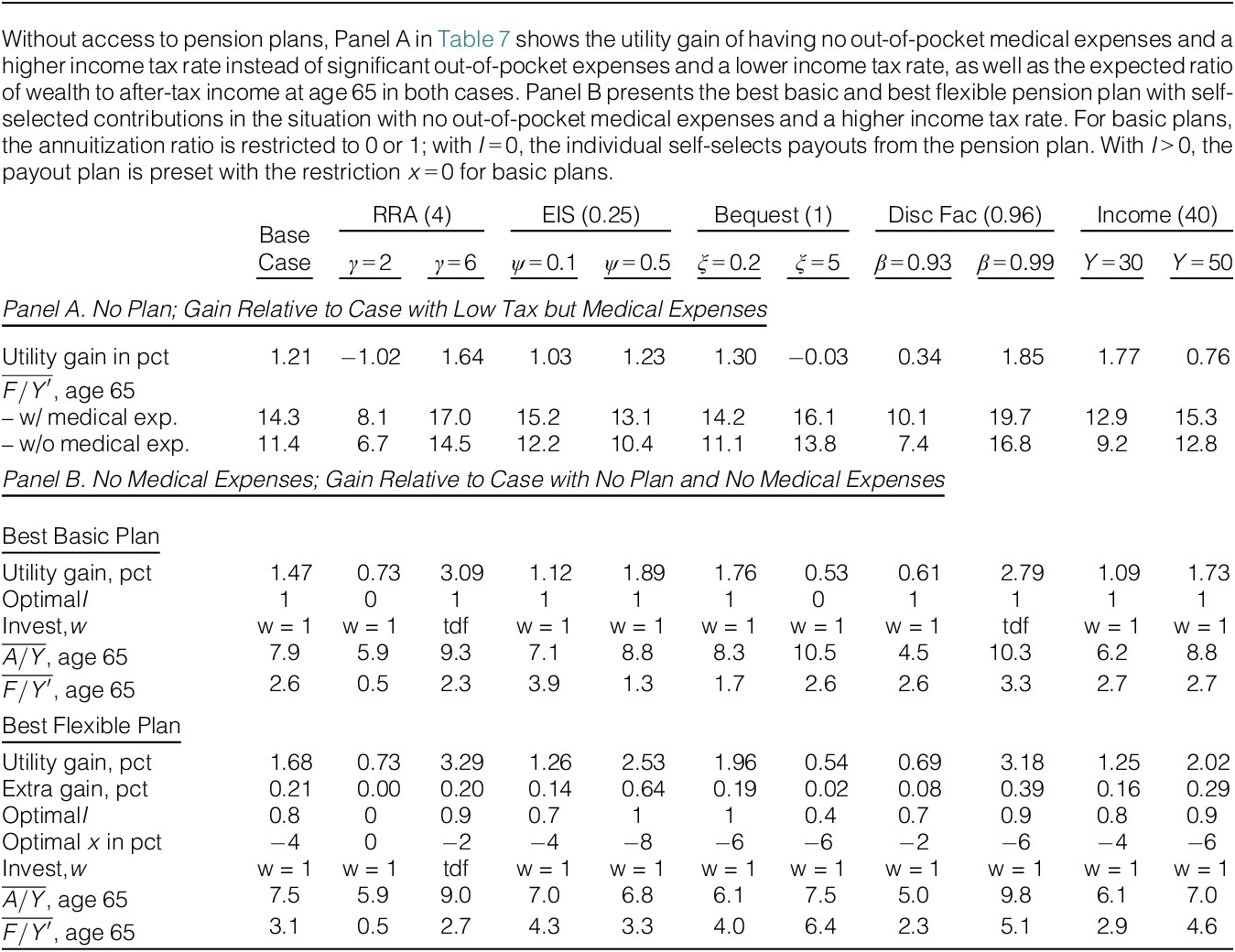
TABLE 7 Long description
Panel A, titled ‘No Plan; Gain Relative to Case with Low Tax but Medical Expenses,’ presents three rows. The first row, ‘Utility gain in pct,’ shows values across columns labeled Base, R R A open parenthesis 4 close parenthesis, E I S open parenthesis 0 dot 25 close parenthesis, Bequest open parenthesis 1 close parenthesis, Disc Fac open parenthesis 0 dot 96 close parenthesis, and Income open parenthesis 40 close parenthesis. Utility gain values range from negative 1 dot 02 to 1 dot 85 percent. The second row, labeled ‘overline F forward slash Y prime, age 65,’ is subdivided into ‘w forward slash medical exp.’ and ‘w forward slash o medical exp.’ For ‘w forward slash medical exp.’, values range from 8 dot 1 to 19 dot 7. For ‘w forward slash o medical exp.’, values range from 6 dot 7 to 16 dot 8. Panel B, titled ‘No Medical Expenses; Gain Relative to Case with No Plan and No Medical Expenses,’ begins with ‘Best basic plan.’ The ‘Utility gain, pct’ row shows values from 0 dot 53 to 3 dot 09. The ‘Optimal I’ row lists values of 0 or 1. The ‘Invest, w’ row mostly shows w equals 1, with some entries as t d f. The ‘overline A forward slash Y, age 65’ row ranges from 4 dot 5 to 10 dot 5. The ‘overline F forward slash Y prime, age 65’ row ranges from 0 dot 5 to 2 dot 7. Next, ‘Best flexible plan’ is presented. The ‘Utility gain, pct’ row ranges from 0 dot 54 to 3 dot 29. The ‘Extra gain, pct’ row ranges from 0 dot 00 to 0 dot 64. The ‘Optimal I’ row ranges from 0 to 1. The ‘Optimal x in pct’ row ranges from negative 8 to 0. The ‘Invest, w’ row again shows w equals 1 or t d f. The ‘overline A forward slash Y, age 65’ row ranges from 5 dot 0 to 10 dot 3. The ‘overline F forward slash Y prime, age 65’ row ranges from 0 dot 5 to 6 dot 4. All columns are consistently labeled as in Panel A.
Panel B of Table 7 displays the best basic and best flexible pension plans with self-selected contributions when medical expenses are tax financed. Utility gains are sizeable, although significantly smaller than in the main setting with out-of-pocket expenses, see Table 6, due to the reduced need for large retirement savings. For the base-case individual, the utility gain is 1.47% instead of 3.19% for basic plans and 1.68% instead of 3.57% for flexible plans. A well-designed pension plan is more valuable to individuals in a U.S.-like system with out-of-pocket medical expenses than in a European-style system with tax-financed medical expenses. Facing less disposable income risk, many of the individuals take more investment risk and prefer plans investing 100% in stocks. When restricted to basic plans, the individual with a high bequest weight now prefers a non-annuitized plan with self-selected payouts to a fully annuitized plan, but this individual marginally prefers a flexible plan with a modest annuitization ratio. With plan flexibility, most individuals still choose a relatively large—although sometimes slightly lower—annuitization ratio and upward-sloping payouts. The flexibility increases the utility gain by up to 0.64 percentage points or $5,514 in PV terms. Also, when equipped with the best pension plan, total retirement savings tend to be somewhat lower with tax-financed medical expenses than without.
B. Tax Incentives and Welfare Considerations
The access to annuitization and tax-free returns on pension savings makes pension plans attractive, whereas the illiquidity of pension savings is the main downside. With pension plans, individuals accumulate less total savings and much less savings in taxed private accounts, so total tax revenue decreases. From a social welfare perspective, the individuals’ utility gains are balanced by the lower tax revenue. I calculate the PV of lifetime taxes on income and returns as the sum of expected tax payments at each age (averaged across simulated paths) discounted using the discount rate applied to income; cf. Section VI.D.
For the base-case individual, the PV of taxes is $433,600 without pension plans. With the optimal basic [flexible] plan, the individual’s utility gain in PV terms is $27,600 [$30,900] while the PV of taxes drops by $37,600 [$36,500], cf. the first row in each panel in Table 8. These numbers question whether such plans improve social welfare, but a full-scale social welfare analysis must include other hard-to-quantify effects excluded from my model. For example, with a pension plan, the individual increases consumption throughout life, which boosts sales tax revenues and employment with ripple effects on corporate and income tax revenue. Also, with sizeable and annuitized savings, retirees draw less on public support.
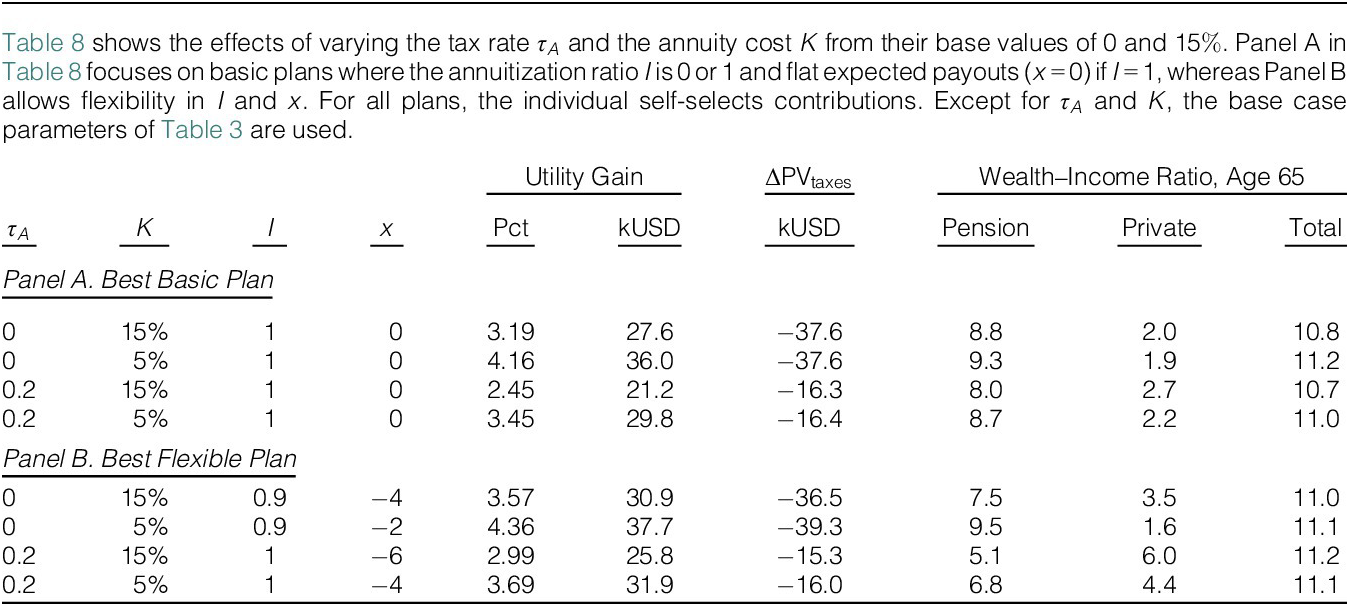
TABLE 8 Long description
Panel A, titled Best Basic Plan, is positioned above Panel B, titled Best Flexible Plan. Panel A contains four rows, each with columns for tax rate tau sub A (values 0), annuity cost K (15 percent or 5 percent), annuitization ratio I (1), expected payout x (0), utility gain (3.19, 4.16, 2.45, 3.45 percent), utility gain in kUSD (27.6, 36.0, 21.2, 29.8), change in present value of taxes Delta P V sub taxes (negative 37.6, negative 37.6, negative 16.3, negative 16.4 kUSD), wealth–income ratio at age 65 split into pension (8.8, 9.3, 8.0, 8.7), private (2.0, 1.9, 2.7, 2.2), and total (10.8, 11.2, 10.7, 11.0). Panel B, below Panel A, also has four rows with columns for tau sub A (0 or 0.2), K (15 percent or 5 percent), I (0.9 or 1), expected payout x (negative 4, negative 2, negative 6, negative 4), utility gain (3.57, 4.36, 2.99, 3.69 percent), utility gain in kUSD (30.9, 37.7, 25.8, 31.9), Delta P V sub taxes (negative 36.5, negative 39.3, negative 15.3, negative 16.0 kUSD), pension (7.5, 9.5, 5.1, 6.8), private (3.5, 1.6, 6.0, 4.4), and total (11.0, 11.1, 11.2, 11.1). The table shows that lower annuity costs and flexible plans yield higher utility gains and wealth–income ratios, while changes in present value of taxes are negative across all scenarios.
The tax advantage is not the main source of the utility gain. Table 8 shows that with a 20% tax rate on all returns, the utility gain of the best basic plan would still be 2.45% (instead of 3.19%) or $21,200 in PV terms, and in this case tax revenues are only $16,300 lower than in the no-plan setting. For the best flexible plan, the gain is $25,800 compared to a reduced tax revenue of $15,300. The utility gains now exceed the drop in taxes. While the overall savings are roughly unchanged, removing the tax exemption leads to lower savings in the pension account and full annuitization of those lower savings becomes optimal (
$ {I}^{\ast } $
 goes from 0.9 to
$ 1 $
goes from 0.9 to
$ 1 $
 ) with a more steeply increasing payout profile (
$ {x}^{\ast } $
) with a more steeply increasing payout profile (
$ {x}^{\ast } $
 goes from
$ -4\% $
goes from
$ -4\% $
 to
$ -6\% $
to
$ -6\% $
 ).
).
The largest source of the utility gain is the access to annuitization, despite the assumed 15% cost. Reducing this to 5%, the gains increase by up to another percentage point or more than $8,000 in PV terms, and the optimal annuitization ratio and pension savings go up (offset by lower private savings), cf. Table 8. Even the RRA 2 individual would then annuitize, with an annuitization ratio of 0.5 and an excess AIR of 2% that generates a 0.95% utility gain, 0.14 percentage points better than the non-annuitized plan with self-selected payouts. Initiatives lowering actual or perceived costs of annuitization could generate substantial utility gains to retirement savers.
C. Heterogeneous Mortality Risk and Annuity Demand
My main analysis applies population mortality rates when calculating annuity payouts and assumes that the individual’s mortality risk is identical to that of the population. What happens if the individual has a different life expectancy than the average individual in the population? I consider a “strong” individual who, at each age until 100, has a probability of dying which is 50% below that of the population and a “weak” [“very weak”] individual with a 50% [150%] higher mortality risk at each age. The top panel of Table 9 shows the implications for the expected lifetime at different ages. When entering retirement at age 67, the average individual expects to live until age 85.0, whereas the very weak, the weak, and the strong individuals expect to live until 78.7, 82.1, and 90.1, respectively.Footnote 18

TABLE 9 Long description
Starting from the top, the table is divided into sections: Expected age at death, No plan, Non-annuitized plan, Best basic plan, and Best flexible plan. Each section contains rows for specific metrics, with columns for Population, Very Weak, Weak, and Strong.
Expected age at death: For age 25, Population 79.8, Very Weak 69.3, Weak 75.3, Strong 87.0. For age 67, Population 85.0, Very Weak 78.7, Weak 82.1, Strong 90.1. For age 80, Population 89.3, Very Weak 85.1, Weak 87.2, Strong 92.9.
No plan: Row for F all over Y prime bar, age 65: Population 14.3, Very Weak 10.9, Weak 13.0, Strong 16.0.
Non-annuitized plan: Utility gain, percent: Population 0.77, Very Weak 0.59, Weak 0.70, Strong 0.84. Row for A all over Y bar, age 65: Population 11.4, Very Weak 8.8, Weak 10.5, Strong 12.5. Row for F all over Y prime bar, age 65: Population 3.7, Very Weak 2.8, Weak 3.3, Strong 4.3. Invest, w: all columns 1.
Best basic plan: Utility gain, percent: Population 3.19, Very Weak 1.16, Weak 2.35, Strong 4.12. Optimal I: all columns 1. Row for A all over Y bar, age 65: Population 8.8, Very Weak 5.6, Weak 7.6, Strong 10.1. Row for F all over Y prime bar, age 65: Population 2.0, Very Weak 3.5, Weak 2.5, Strong 1.6. Invest, w: all columns t d f.
Best flexible plan: Utility gain, percent: Population 3.57, Very Weak 1.23, Weak 2.53, Strong 4.96. Optimal I: all columns 0.9. Optimal x in percent: Population minus 4, Very Weak minus 2, Weak minus 4, Strong minus 6. Row for A all over Y bar, age 65: Population 7.5, Very Weak 5.3, Weak 6.3, Strong 7.5. Row for F all over Y prime bar, age 65: Population 3.5, Very Weak 3.9, Weak 4.1, Strong 4.2. Invest, w: all columns t d f.
Table 9 confirms that the strong individual with a higher-than-average expected lifetime benefits more from annuities. For flexible plans, the utility gain is 4.96% for the strong individual compared to 3.57% for an individual with an average mortality. With a gain of 1.23%, even the very weak individual benefits from annuitization. Despite the assumed 15% costs, full or partial annuitization is attractive even to individuals with a considerably lower expected lifetime than assumed in the calculation of annuity payouts. The weaker individuals build up less total retirement savings and keep a smaller fraction of their overall savings in the pension account. All the individuals choose an annuitization ratio of 0.9, whereas the desired payout profile is more steeply increasing for individuals with longer expected lifetimes.
D. Option to Make Unscheduled Withdrawals
As an extension, I now allow the individual at the beginning of each year
$ t $
 to choose a fraction
$ {M}_t\ge 0 $
to choose a fraction
$ {M}_t\ge 0 $
 of the pension account
$ {A}_t $
of the pension account
$ {A}_t $
 to be paid out in addition to any scheduled payouts. To obtain an unscheduled cash payout of
$ {M}_t{A}_t $
to be paid out in addition to any scheduled payouts. To obtain an unscheduled cash payout of
$ {M}_t{A}_t $
 , the value of the annuity portfolio is reduced by
$ \left(1+{k}_t\right){M}_t{A}_t $
, the value of the annuity portfolio is reduced by
$ \left(1+{k}_t\right){M}_t{A}_t $
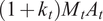 , where
$ {k}_t\ge 0 $
, where
$ {k}_t\ge 0 $
 reflects a cost or penalty. For 401(k)s in the United States, a 10% tax penalty is paid on withdrawals before the age of 59.5 years.Footnote
19 In addition, I assume a cost equal to 1% of any unscheduled payout to represent any actual and psychological burdens related to obtaining such payouts. Then I also avoid any simultaneous contributions and withdrawals from age 60 to retirement. Hence, I let
$ {k}_t=0.11 $
reflects a cost or penalty. For 401(k)s in the United States, a 10% tax penalty is paid on withdrawals before the age of 59.5 years.Footnote
19 In addition, I assume a cost equal to 1% of any unscheduled payout to represent any actual and psychological burdens related to obtaining such payouts. Then I also avoid any simultaneous contributions and withdrawals from age 60 to retirement. Hence, I let
$ {k}_t=0.11 $
 for
$ t\le 60 $
for
$ t\le 60 $
 and
$ {k}_t=0.01 $
and
$ {k}_t=0.01 $
 for
$ t>60 $
for
$ t>60 $
 . See Section IA.5 of the Supplementary Material for additional information.
For the base-case individual, the withdrawal option increases the utility gain associated with the best basic pension plan marginally from 3.19% to 3.28%. Early withdrawals occur only when the individual has a relatively high pension wealth (large
$ a $
 ) and low income (small
$ y $
) and low income (small
$ y $
 ). At each age below 60, no early withdrawals occur in more than 95% of the simulations. After age 60, early withdrawals are more common but typically small; in more than 95% of the simulations, the maximum unscheduled withdrawal is less than $300.
The withdrawal option has a more notable impact on flexible plans. With this option, the base-case individual prefers a steeper payout profile with an excess AIR of
$ -8\% $
 instead of
$ -4\% $
instead of
$ -4\% $
 . The scheduled payouts can be more backloaded since the individual can make early unscheduled payouts when needed, thus making the total payouts state dependent. The optimal annuitization ratio remains unchanged at 0.9. Adding the withdrawal option increases the utility gain for the best flexible plan from 3.57% to 3.85%, an increase corresponding to around $2,377 in PV terms. On the other hand, the withdrawal option complicates the risk management procedures of the annuity provider and may thus lead to a larger annuity cost. If the withdrawal option causes the cost to increase from 15% to 19% or more, the utility gain is indeed lower with the option than without.
VII. Conclusion
In a rich life-cycle model, I show that the access to well-designed retirement saving plans greatly improves the utility of rational workers across a range of individual characteristics. The utility gains are due to the access to annuitization (despite significant costs) and a return tax advantage, and the gains are significantly increased if the plans allow for partial annuitization, non-flat payout schedules, and maybe also early withdrawal options if this flexibility does not considerably increase annuity costs. Most of the individuals prefer a target-date fund investment strategy, pension payouts that are expected to increase through retirement, as well as a large degree of (but less than full) annuitization of their retirement savings. Individuals’ optimal contributions to the retirement saving plans are typically small early in working life and then increase slowly with age until the final years before retirement, where optimal contributions tend to be large. Whether the possibly large medical expenses in retirement are tax-financed or paid out of the individual’s own pockets matters for which retirement saving plan is best and how big the associated utility gain is.
Various extensions of my model seem interesting to explore. First, while the Vanguard-style target-date fund strategy included in my study is preferred by many of the individuals considered, alternative specifications of the strategy might be even better, for example, with a larger stock weight in the final part of the strategy or a different period over which the stock weight is reduced. Second, additional individual characteristics (such as home ownership and thus the possible saving through home equity accumulation) and alternative preferences (such as habit formation) could be investigated, although at significant computational costs.
Supplementary Material
To view supplementary material for this article, please visit http://doi.org/10.1017/S0022109026102968.
Funding Statement
Support from the Danish Finance Institute (DFI) is gratefully acknowledged. I also appreciate support from the pension research center PeRCent which receives base funding from Danish pension funds and Copenhagen Business School.











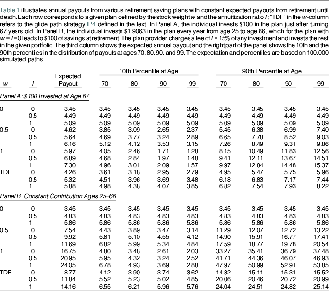
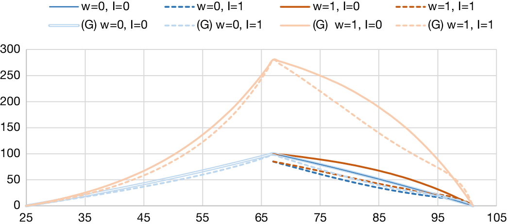


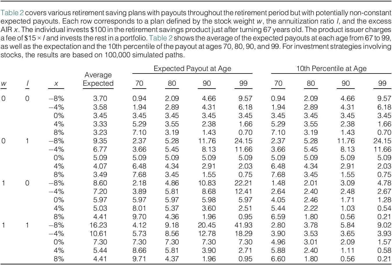
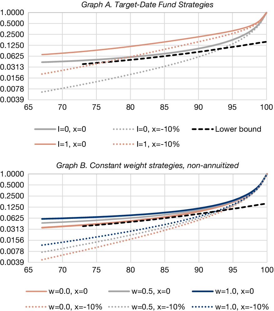


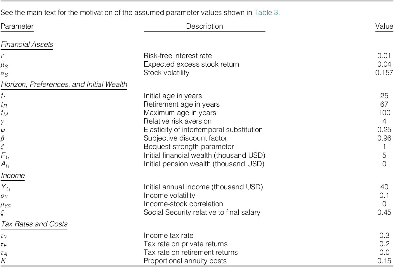
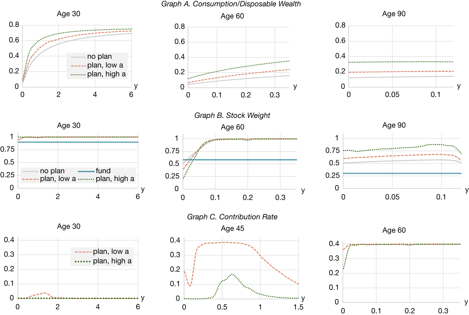


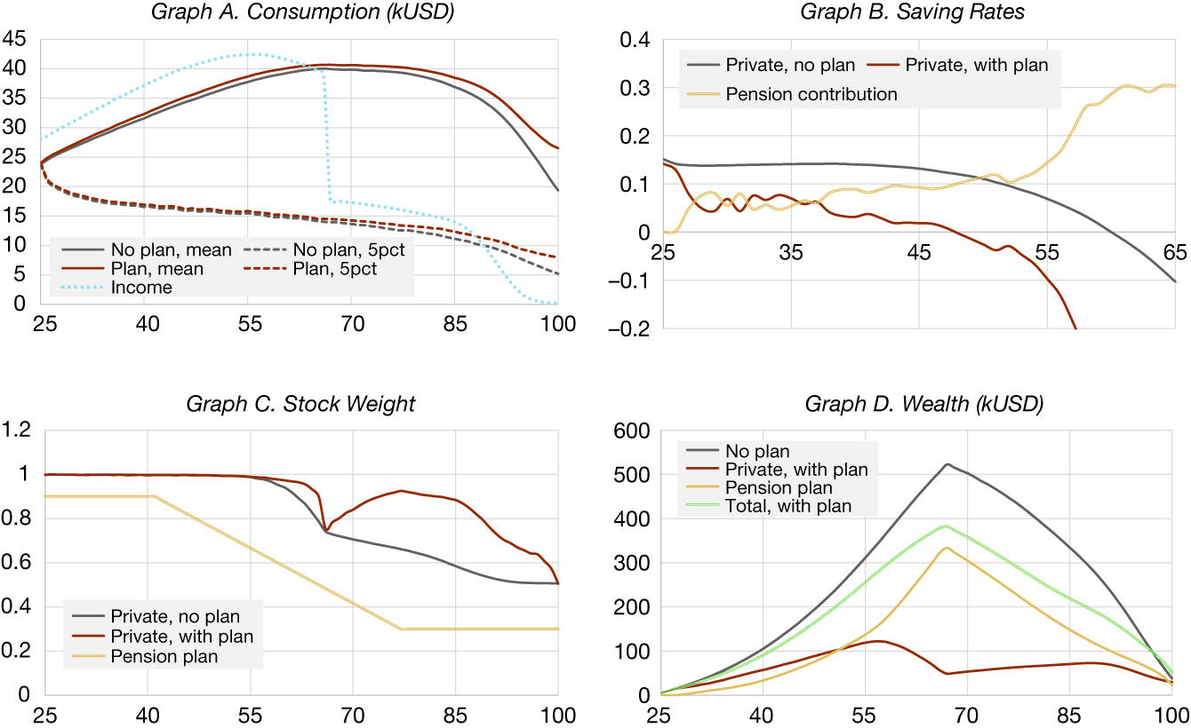
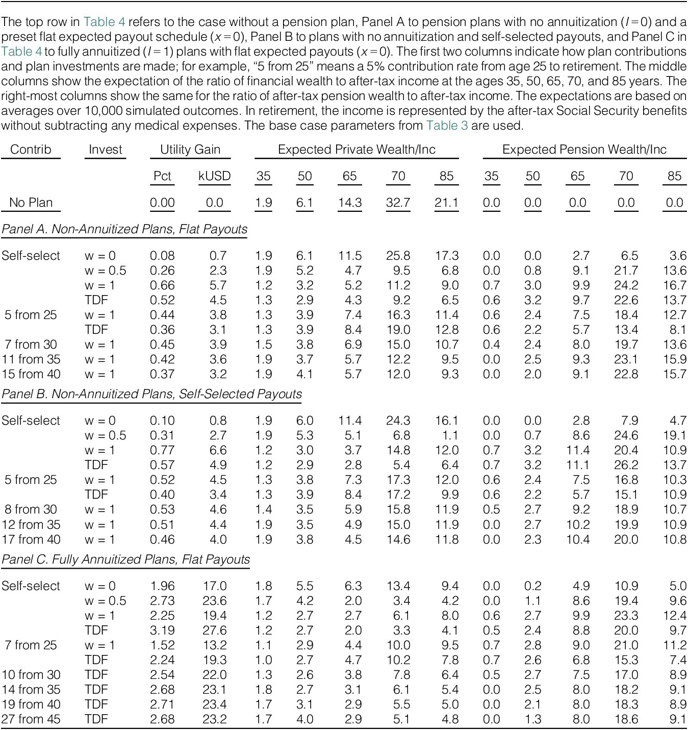
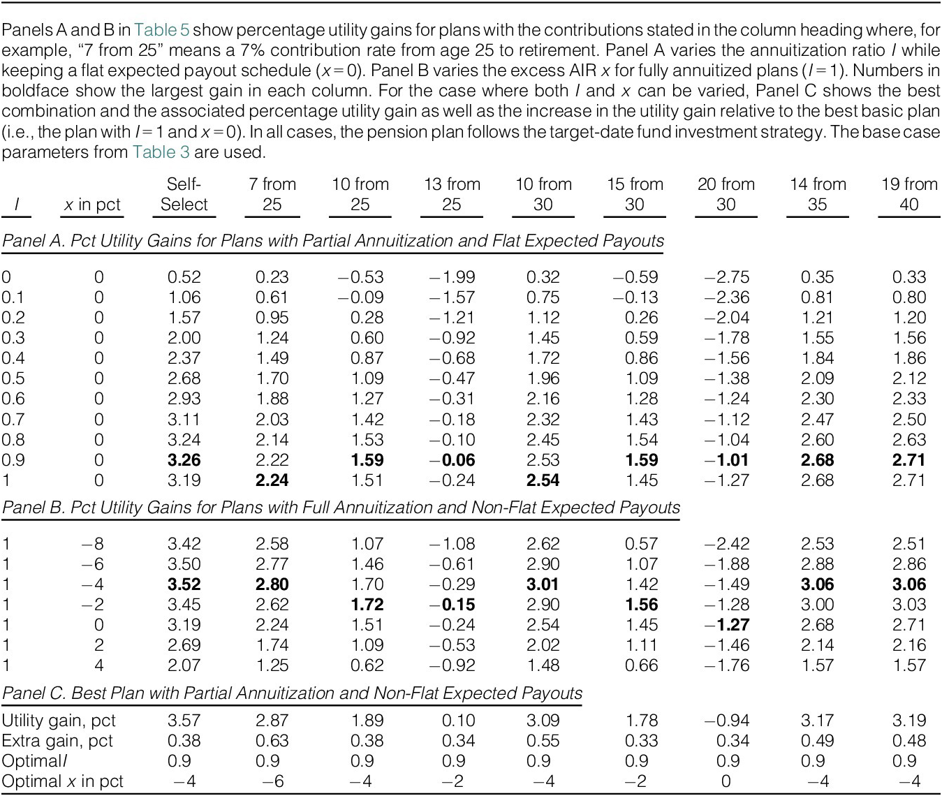
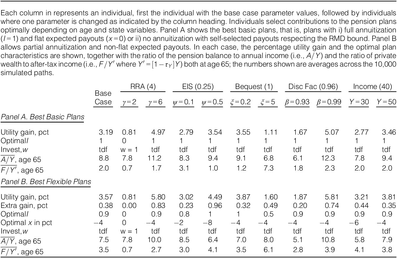
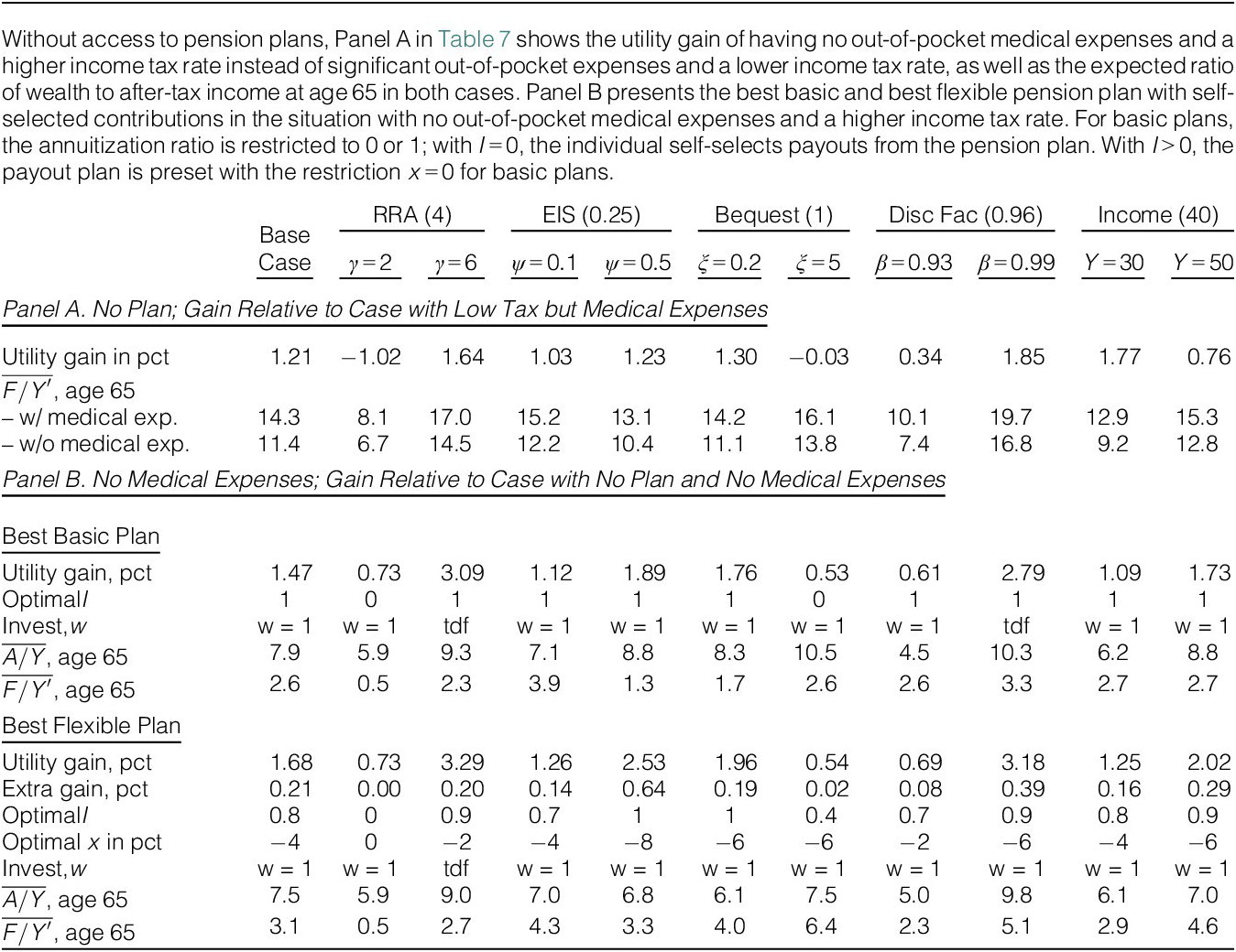
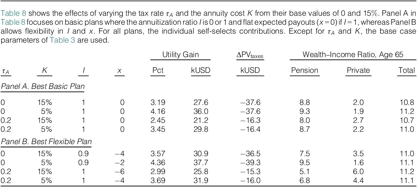
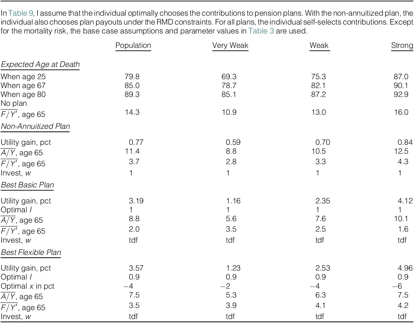


 Open access

