3.1. Instantaneous and mean flows

Figure 3(a) shows the streamwise component of the instantaneous velocity field in one of the snapshots collected. The uniform free stream of the inflow is disrupted by the irregularly arranged ligaments of the solid structure and velocity fluctuations arise within the porous matrix. Vortices of different orientations are shed from the ligaments and a wake is formed. The largest perturbations are observed close to the downstream edge of the porous matrix. The wakes originated by the ligaments develop in a non-uniform fashion and interact at variable lengths. The smaller wakes are seen to disappear after a couple of pore diameters, whereas larger wakes stemming from ligament clumps meet at a further distance from the foam. The larger wakes also last in time, as revealed by the streaks in the time-averaged velocity field $\langle U \rangle _t$ shown in figure 3(b).

Figure 3.

Instantaneous velocity field of the streamwise velocity component (a) and its temporal mean (b) in an $x$–$y$ plane.

3.2. Homogeneity and isotropy

The approximation to statistical homogeneity in the cross-flow directions in grid turbulence is known to depend on the grid geometry and the Reynolds number. While, for regular grids, experiments suggest that the flow becomes nearly homogeneous for $x/M > 40$ (Comte-Bellot & Corrsin Reference Comte-Bellot and Corrsin1966; Mohamed & Larue Reference Mohamed and Larue1990), for fractal grids, homogeneity is usually retrieved further downstream (Hearst & Lavoie Reference Hearst and Lavoie2014) and, for example, Valente & Vassilicos (Reference Valente and Vassilicos2011) report $x/M_{{eff}}>80$, where $M_{{eff}}$ is the effective mesh size.

The distribution of $\langle U \rangle _t$ in cross-flow planes is shown in figure 4 for six streamwise positions at increasing distance from the metal foam. Solid lines mark regions where the percentage of variation of $\langle U \rangle _t$ relative to $U_{\infty }$ has magnitude greater than $10\,\%$, while dashed lines encompass regions of magnitude greater than $5\,\%$. These are seen to gradually shrink along $x$. While inhomogeneity is in part to be ascribed to the limited size of the sample composed only by the collection of snapshots in time, for $x > 20$ their extent is still appreciable. In the $x = 30$ station, the time-averaged velocity $\langle U \rangle _t$ varies between $0.86$ and $1.12$.

Figure 4.

Streamwise mean flow field $\langle U \rangle _t$ in $y$–$z$ planes extracted at $x=5$, $10$, $15$, $20$, $25$ and $30$ (left to right then top to bottom): solid line, isolines $\langle U \rangle _t - U_{\infty } = \pm 0.1$; and dashed line, isolines $\langle U \rangle _t - U_{\infty } = \pm 0.05$.

The isotropy level of the large scales of motion can be investigated through the ratio of root-mean-square (r.m.s.) velocity fluctuations along orthogonal directions. In the present case, the fluctuations of the $x$-component of velocity are the largest: in the developed region, indicators $u_{rms}/w_{rms}$ and $u_{rms}/v_{rms}$ oscillate within the interval $(1.5, 1.6)$ about a mean of 1.55 for $u_{rms}/v_{rms}$ and 1.56 for $u_{rms}/w_{rms}$, where the difference is finally due to the size of the sample employed in the simulations. In previous grid turbulence measurements (Kurian & Fransson Reference Kurian and Fransson2009; Krogstad & Davidson Reference Krogstad and Davidson2010; Kitamura et al. Reference Kitamura, Nagata, Sakai, Sasoh, Terashima, Saito and Harasaki2014), the observed isotropy indicators are in general smaller than those measured here. Kitamura et al. (Reference Kitamura, Nagata, Sakai, Sasoh, Terashima, Saito and Harasaki2014), who also collected experimental results by other authors, report $u_{rms}/w_{rms} < 1.2$ in all cases; similar values are also reported in the lee of fractal grids (Hurst & Vassilicos Reference Hurst and Vassilicos2007; Gomes-Fernandes, Ganapathisubramani & Vassilicos Reference Gomes-Fernandes, Ganapathisubramani and Vassilicos2012). More details about large-scale isotropy measures downstream of the present metal foam are reported in Corsini & Stalio (Reference Corsini and Stalio2020).

3.3. Decay of velocity fluctuations

Figure 5 displays the streamwise evolution of the variance of the three components of velocity $\langle u_i u_i\rangle$ as well as the turbulent kinetic energy $\langle k \rangle$. Very close to the foam and for $x < 1$, velocity fluctuations are observed to remain constant. The negative slope increases gradually in $x$ until fluctuations exhibit a power-law decay that persists until the end of the computational domain. As demonstrated, for example, in Tennekes & Lumley (Reference Tennekes and Lumley1972), this is expected in the region where advection and dissipation of the turbulent kinetic energy become the only non-negligible terms in the transport equation of $\langle k \rangle$; see § 3.10.

Figure 5.

Decay of velocity fluctuations: solid line, $\langle uu\rangle$; dot-dashed line, $\langle vv\rangle$; dotted line, $\langle ww\rangle$; and dashed line, $\langle k \rangle$.

Power-law parameters are sought in the form

(3.1)\begin{equation} \frac{u_{rms}^2}{U_{\infty}^2}= A \left(\frac{x-x_0}{d_p} \right)^{{-}n} \end{equation}

through a numerical procedure. In (3.1), $A$ is the multiplicative coefficient, $x_0$ is the virtual origin and $n$ is the decay exponent. As $n$ is positive, the power law has a vertical asymptote (and a singularity) at the virtual origin $x = x_0$. As the parameters in (3.1) depend greatly upon the interval of sampling data considered, also the interval limits are determined inside the fitting procedure. A similar approach has been applied in Hearst & Lavoie (Reference Hearst and Lavoie2014).

In the present work, a developed region $I_d = [x_{min}, x_{max} ]$ is employed, where the right border of the interval is kept fixed to $x_{max} = 30.0$, clear of possible – yet not evident – outflow condition effects, while $x_{min}$ is discretely varied in the interval $[0.015, 24.7]$ to seek an $x_{min}$ coordinate that ensures the best fit. The coordinate $x_{min}$ will be taken as the start of the developed region. For each selection of a value for $x_{min}$, the virtual origin $x_0$ is discretely varied within $I_0 = [0.015, x_{min}]$, as the singularity is not supposed to belong to $I_d$. The intervals of variation of both $x_{min}$ and $x_0$ are discretised by the same subdivision as the computational mesh. Parameters $A$ and $n$ are determined through a least-squares fit. Deviations between computed data and fitting laws are then calculated as the Euclidean norm of the error divided by the number of data points:

(3.2)\begin{equation} e(x_0,x_{min}) = \frac{\left( \displaystyle{\sum\nolimits_{j=1}^{N_d}} \delta^2_j \right)^{1/2}}{N_d}. \end{equation}

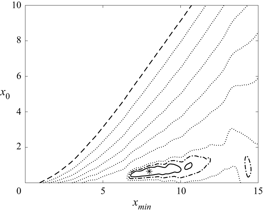
In (3.2), $\delta _j$ represents the difference between computed statistics and the least-squares fitted power-law approximation of $u_{rms}^2$ at the $j$th point of $I_d$; and $N_d$ is the number of uniformly spaced points in the data fit region $I_d$. The $(x_0,x_{min})$ couple which ensures the smallest deviation from computed data provides the final $A$ and $n$ coefficients. This procedure leads to the results given in table 2 with error distribution as in figure 6. In the region of parameters investigated, only one minimum is found, which is located far from the boundaries of the region investigated. The dependence on porosity of the power-law exponents obtained is shown to be only weak in the Appendix.

Figure 6.

Contour lines of $\log _{10}(e)$, where $e$ is the normalised Euclidean norm of the error in (3.2): dashed line, $\log _{10}(e) = -4.8$; dot-dashed line, $\log _{10}(e) = -6.03$; solid line, $\log _{10}(e) = -6.05$; and dotted line, $\log _{10}(e) \in [-6.00 -5.00]$, with lines separated by $\delta = 0.2$. A single minimum is found in the field, as indicated by the $*$ symbol, which corresponds to $x_0 = 0.648$ and $x_{min} = 7.98$. The singularity is not included in the domain, and thus $x_{min} > x_0$.

Table 2.

Left boundary of the fitting interval $I_d$, virtual origin, multiplicative coefficient and decay exponent of the power laws in the form of equation (3.1) fitting $u_{rms}^2$ and $\langle k \rangle$.

In order to check the dependence of the results from the fitting method employed, a procedure from the literature is also applied to the same set of data; this alternative technique is that utilised by Hearst & Lavoie (Reference Hearst and Lavoie2014). In the application of the method to the present case, the virtual origin $x_0$ and lower bound $x_{min}$ are varied within $I_0 = [0, 4]$ and $[4, 14.7]$, respectively. For both $u_{rms}^2$ and $\langle k \rangle$, the process converges after three iterations. Applied to $u_{rms}^2$, this fitting procedure provides $x_0=0.610$ and $x_{min}=6.78$, which yield the estimate for $\tilde {n}_u = 1.12$. In the case of $\langle k \rangle$, the values obtained are $x_0=0.360$, $x_{min}=5.02$ and $\tilde {n}_k=1.14$. The results obtained by the method proposed by Hearst & Lavoie (Reference Hearst and Lavoie2014) are only marginally different from those obtained as described above and reported in table 2.

Comte-Bellot & Corrsin (Reference Comte-Bellot and Corrsin1966) found $1.15\leqslant n \leqslant 1.29$ for regular grids, while according to Mohamed & Larue (Reference Mohamed and Larue1990) $n \approx 1.3$. More recently, Krogstad & Davidson (Reference Krogstad and Davidson2010) found $n = 1.13 \pm 0.02$.

Besides the parameters $x_0$, $A$ and $n$ in (3.1), the procedure provides the coordinate $x_{min}$ of the start of the developed region as the left boundary of the interval $I_d$. All the subsequent fittings in this work will be carried out on $I_d = [7.98, 30.0]$.

3.4. Turbulence decay rate

As opposed to experimental studies, where rate of dissipation $\langle \epsilon \rangle$ needs to be evaluated using the frozen turbulence assumption or isotropy (3.5), in DNS studies $\langle \epsilon \rangle$ can be computed directly from its definition,

(3.3)\begin{equation} \langle\epsilon\rangle \equiv \frac{2}{{\textit{Re}}_{d_p}} \langle s_{ij} s_{ij} \rangle, \end{equation}

where $s_{ij} = ( \partial u_i/\partial x_{j} + \partial u_j/\partial x_{i} )/{2}$ is the fluctuating rate of strain. Figure 7 displays the spatial evolution of $\langle \epsilon \rangle$, together with the least-squares fitted power law in the form $\langle \epsilon \rangle \sim a_{\epsilon } x^h$. The coefficients that fit the data over $I_d = [7.98, 30.0]$ are $a_{\epsilon } = 0.217$ and $h = -2.20$.

Figure 7.

Dissipation of the turbulent kinetic energy: dashed line, $\langle \epsilon \rangle$ as defined in (3.3); dotted line, $\langle \epsilon \rangle _{iso}$ from (3.5); and solid line, $a_\epsilon x^h$, with $a_\epsilon = 0.217$ and $h = -2.20$.

The scaling of dissipation $\langle \epsilon \rangle$ can also be set in relation to the scaling of $\langle k \rangle$ in § 3.3. As also shown quantitatively in § 3.10, in the developed region of a statistically steady, high-Reynolds-number flow, one has

(3.4)\begin{equation} \langle U \rangle \frac{\mathrm{d} k}{\mathrm{d} x} ={-} \langle\epsilon\rangle. \end{equation}

Equation (3.4) suggests that the decay exponent in this case should equal $h = - (n_k +1)$. In the present study, $h = -2.20$ and $n_k = 1.14$ are calculated. The percentage difference between $- (n_k + 1)$ and $h$ is below 3 %.

Dissipation is compared in figure 7 to the same quantity computed under the hypothesis of isotropic turbulence:

(3.5)\begin{equation} \langle\epsilon\rangle_{iso} = 15 \nu \left\langle \left( \frac{\partial u}{\partial x} \right)^2 \right\rangle. \end{equation}

The close similarity between $\langle \epsilon \rangle$ and $\langle \epsilon \rangle _{iso}$ is only in apparent contradiction with isotropy ratios larger than 1.5 reported in § 3.2. From the demonstration by Taylor (Reference Taylor1935), it appears that hypotheses less strict than isotropy are required for equation (3.5) to hold. The weaker set of hypotheses hold true in the present case; see Corsini & Stalio (Reference Corsini and Stalio2020).

3.5. Length scales

The length scales examined for the characterisation of the turbulence generated by a metal foam are the Kolmogorov scale $\eta$, the Taylor microscale $\lambda$ and the integral scales. All the length scales are computed directly from their definitions. Their distribution within the developed region is approximated by a power law of the distance $x$. The range of variation of each length scale along $I_d$ is reported in table 1 together with data from the literature on classical grid turbulence.

3.5.1. Kolmogorov scale

The Kolmogorov scale is defined through dissipation $\langle \epsilon \rangle$. It is predicted from the power-law expression for $\langle \epsilon \rangle$ (derived from the expression for $\langle k \rangle$) that $\eta$ can be represented by a function of the form $\eta \sim a_\eta x^s$, where $s$ equals $-h/4$ and finally $s = (n_k + 1)/4$. The decay exponent for $\langle k \rangle$ computed here, $n_k = 1.14$, gives $s = 0.54$. The power-law approximation is displayed in figure 8 together with the Kolmogorov scale, as computed from its definition: the fitting coefficients are $a_\eta = 0.00291$ and $s = 0.55$. Very similar power-law parameters are obtained in this same flow configuration for a porosity $\varepsilon = 0.97$; see the Appendix. Comte-Bellot & Corrsin (Reference Comte-Bellot and Corrsin1971) provide Kolmogorov-scale measurements in their table 4, which grow like a power law of exponent $\hat {s} = 0.58$.

Figure 8.

Streamwise distribution of the Kolmogorov scale: dashed line, $\eta$ as calculated from its definition; and solid line, $a_\eta x^s$, where $a_\eta = 0.00291,\ s = 0.55$. The uniform grid spacing adopted in all directions is $\Delta x_i = 0.0146$, which suggests that spatial resolution is high enough to represent the smallest scales of the turbulence.

3.5.2. Taylor microscale

Figure 9 displays the streamwise distribution of the Taylor microscale, defined by

(3.6)\begin{equation} u_{rms}^2 = \lambda^2 \left\langle\left( \frac{\partial u }{\partial x} \right)^2\right\rangle. \end{equation}

Comte-Bellot & Corrsin (Reference Comte-Bellot and Corrsin1971) report Taylor-scale values in a few measurement points (see their table 4); their data fit a power law of exponent $c = 0.53$. It is predicted in the study by George (Reference George1992) that the Taylor scale of homogeneous isotropic turbulence increases in time with $t^{1/2}$ and, for grid turbulence, $\lambda$ grows as $x^{1/2}$ in the laboratory frame. More recently, Kurian & Fransson (Reference Kurian and Fransson2009) reported that $\lambda$ increases approximately like the square-root of the streamwise coordinate. In the present study, fitting a power-law approximation of the form $\lambda \sim a_\lambda x^c$ over $I_d$ gives $a_\lambda = 0.0577$ and $c = 0.52$.

Figure 9.

Streamwise distribution of the Taylor microscale: dashed line, $\lambda$ as calculated from its definition; and solid line, $a_\lambda x^c$, where $a_\lambda = 0.0577$ and $c = 0.52$.

Figure 10 shows the behaviour of the turbulent Reynolds number. After a steep decrease in the vicinity of the metal foam, ${\textit {Re}}_{\lambda }$ reaches a plateau where ${\textit {Re}}_{\lambda } \approx 80$. An expression relating the Taylor and the Kolmogorov scales can be obtained for isotropic turbulence through (3.5):

(3.7)\begin{equation} \frac{\lambda}{\eta}=15^{1/4} {\textit{Re}}_{\lambda}^{1/2}. \end{equation}

Results from the present investigation, and not reported for brevity, show that the difference between $( \lambda / \eta )^2 / \sqrt {15}$ and ${\textit {Re}}_{\lambda }$ is less than 3 % over the whole computational domain.

Figure 10.

Streamwise distribution of ${\textit {Re}}_{\lambda }$. The horizontal dashed line specifies the value ${\textit {Re}}_{\lambda } = 80$.

3.5.3. Integral scales

The autocorrelation coefficient is defined as the ratio between the autocorrelation function of separation $\boldsymbol {r} = r \boldsymbol {e}_{j}$ and the autocorrelation function for $r = 0$:

(3.8)\begin{equation} \rho_{ii}(x, \boldsymbol{r}) = \frac{ R_{ii}(x, \boldsymbol{r}) }{ R_{ii}(x, 0) }. \end{equation}

The autocorrelation coefficients along $y$ of the streamwise $\rho _{11}(x,r \boldsymbol {e}_{2})$ and the cross-flow $\rho _{22}(x,r \boldsymbol {e}_{2})$ velocity components are reported in figure 8 of Corsini & Stalio (Reference Corsini and Stalio2020). A distinction is made between the transverse and longitudinal correlations depending on the relative direction of velocity components and separation vector. Transverse correlations built with streamwise velocity fluctuations have longer tails with respect to longitudinal correlations built with spanwise fluctuations.

Integral scales are defined as integrals over $r$ of autocorrelation coefficients:

(3.9)\begin{equation} L_{ii} (x,\boldsymbol{e}_{j}) = \frac{1}{R_{ii}(x,0)}\,\int_{0}^{\infty} R_{ii}(x,r \boldsymbol{e}_{j})\, \mathrm{d} r. \end{equation}

These depend upon the coordinates along non-homogeneous directions as well as on the direction of separation $\boldsymbol {e}_{j}$. In practice, since the computational domain has finite boundaries, the integral scales are calculated here as the distance over which the autocorrelation function decreases from $1$ to $1/\textrm {e}$, where $\textrm {e}$ is Euler's number. For the calculation of integral scales, correlations are assumed to decay exponentially.

Integral scales for the present case are based on the streamwise or the cross-flow velocity components. Given the inhomogeneity of the streamwise direction, separation is set in the cross-flow directions $\boldsymbol {e}_{2}$ and $\boldsymbol {e}_{3}$. Thus, the integral scale based on the streamwise velocity is always transverse and will be denoted by $L$. The integral scales based on cross-flow velocity components can be either longitudinal or transverse and are denoted by $L_g$ and $L_t$, respectively. As statistically $L_{11} (x,\boldsymbol {e}_{2}) = L_{11} (x,\boldsymbol {e}_{3}) = L (x)$, $L_{22} (x,\boldsymbol {e}_{2}) = L_{33} (x,\boldsymbol {e}_{3}) = L_g (x)$ and $L_{33} (x,\boldsymbol {e}_{2}) = L_{22} (x,\boldsymbol {e}_{3}) = L_t (x)$, these equalities have been exploited in the calculation of integral scales.

Figure 11 displays the integral scales. The power-law approximations $L \sim a_L x^q$ have the coefficients reported in table 3; the exponents computed are very close to the $L \sim x^{1/2}$ behaviour predicted by Wang & George (Reference Wang and George2002). Also, in the case of higher porosity presented in the Appendix, the power-law exponent is close to $1/2$.

Figure 11.

Streamwise distribution of the integral scales: dot-dashed line, streamwise integral scale $L$; dashed line, longitudinal integral scale $L_g$; dotted line, transverse integral scale $L_t$; and solid line, power-law approximations of the different scales.

Table 3.

Parameters of the power-law functions of the form $f(x) \sim a x^b$ fitting the turbulent quantities analysed.

Notice that $L$ is one order of magnitude smaller than the domain size, the transverse length of which is $11.25 d_p$; this suggests that the imposed lateral periodic boundary conditions can satisfactorily represent cross-flow homogeneity in the present case. The evolution of the Reynolds number based on the integral scale, defined as ${\textit {Re}}_{L} \equiv L u_{rms} /\nu$, along the $x$-axis is displayed in figure 9 of Corsini & Stalio (Reference Corsini and Stalio2020).

3.6. Dissipation rate coefficient

In high-Reynolds-number turbulent flows away from solid walls, the dissipation rate can be scaled on the integral length scale and velocity fluctuations through an order-one constant:

(3.10)\begin{equation} C_{\epsilon} = \frac{\langle\epsilon\rangle L}{u_{rms}^{3}}. \end{equation}

Figure 12 shows that, in the present case, after an initial steep increase for $x < 2$, the dissipation rate coefficient $C_{\epsilon }$ based on $L$ fluctuates over $I_d$ between $0.45$ and $0.50$, where its spatial average is $\bar {C}_{\epsilon } = 0.483$. This value is very close to values reported in Pearson, Krogstad & van de Water (Reference Pearson, Krogstad and van de Water2002) for shear turbulence at different ${\textit {Re}}_\lambda$ numbers.

Figure 12.

Streamwise distribution of $C_{\epsilon } = {\langle \epsilon \rangle L}/{u_{rms}^{3}}$: solid line, based on the streamwise integral scale $L$; dashed line, based on the longitudinal integral scale $L_g$; and dotted line, based on the transverse integral scale $L_t$.

With regard to the initial steep increase, in recent years Vassilicos and coworkers have observed that, close to the turbulence-generating grid, there is a region characterised by spectra that closely match the ${-5/3}$ power law, in conjunction with an increase in $C_\epsilon$. In the hypothesis of $\langle \epsilon \rangle = \langle \epsilon \rangle _{iso}$, combining the definition (3.10) with equation (3.5) leads to

(3.11)\begin{equation} C_{\epsilon} = 15\, \frac{L}{\lambda} \frac{1}{{\textit{Re}}_{\lambda}}. \end{equation}

As only small variations of the ratio between length scales $L/\lambda$ are observed for given Reynolds number of the mesh size, $C_{\epsilon }$ is seen to increase like ${\textit {Re}}_{\lambda }^{-1}$. This behaviour is reported for both fractal and regular grids (Valente & Vassilicos Reference Valente and Vassilicos2012).

Equation (3.11) is studied for the present case in figure 13, where the logarithmic plot emphasises the $C_{\epsilon } (Re_{\lambda })$ behaviour close to the metal foam. Corresponding to the initial steep decrease in ${\textit {Re}}_{\lambda }$ shown in figure 10, $C_\epsilon$ is seen to increase like $Re_{\lambda }^{-1}$. In the same region, a well-defined $-5/3$ energy spectra behaviour is observed over a broader wavenumber range than the fully developed region; see the inset of figure 15 in § 3.8. The situation described in Valente & Vassilicos (Reference Valente and Vassilicos2012) is thus observed in the present case.

Figure 13.

Plot of $C_{\epsilon }$ as a function of $Re_{\lambda }$. The dashed line follows $Re_{\lambda }^{-1}$.

The streamwise evolution of $C_\epsilon$ experiences a transition between the $Re_{\lambda }^{-1}$ behaviour and a region where the variations in $C_\epsilon$ are much smaller; see figures 12 and 13. This transition is about $x = 2$. The turbulent kinetic energy budgets reported in § 3.10 indicate that, downstream of this location, the turbulent transport terms become negligible and the mean advection of $\langle k \rangle$ equals dissipation. On the contrary, for $x<2$, this equality does not hold, and the variations of $C_\epsilon$ suggest a non-equilibrium condition between energy at the large scales and dissipation. It should be noted that the present results confirm the predictions reported by Tennekes & Lumley (Reference Tennekes and Lumley1972) in their (3.2.29) and (3.2.30), where transition is expected at streamwise distances from the grid that are much larger than the integral scale. In the present configuration, $x = 2$ corresponds to $x \approx 6 L$.

In the theory by Richardson and Kolmogorov, the constancy of $C_\epsilon$ requires that turbulence is at a high Reynolds number and far from solid walls. While the small variations of $C_\epsilon$ in the fully developed region can be attributed to the Reynolds number, which is not very high, the steep increase in $C_\epsilon$ in the vicinity of the porous matrix ($x < 2$) is to be ascribed to the vicinity of the solid filaments and ultimately to non-negligible turbulent transport terms in the budget equation of $\langle k \rangle$.

3.7. Is grid turbulence Saffman turbulence?

In recent articles (Krogstad & Davidson Reference Krogstad and Davidson2010; Kitamura et al. Reference Kitamura, Nagata, Sakai, Sasoh, Terashima, Saito and Harasaki2014) it was discussed whether grid turbulence can be considered to be of the Saffman type. Both Krogstad & Davidson (Reference Krogstad and Davidson2010) and Kitamura et al. (Reference Kitamura, Nagata, Sakai, Sasoh, Terashima, Saito and Harasaki2014) conclude that grid turbulence is Saffman turbulence.

The theory by Saffman (Reference Saffman1967) describes the decay of homogeneous turbulence as

(3.12a,b)\begin{equation} u_{rms}^2 = K C^{{2}/{5}} t^{-{6}/{5}}, \quad L = K^\prime C^{{1}/{5}} t^{{2}/{5}}, \end{equation}

where $K$ and $K^\prime$ are constants and $C$ is expressed by an invariant integral. Both equations (3.12a,b) have to hold for turbulence to be of the Saffman type. This is sometimes expressed by the requirement that $u_{rms}^2 L^3 = \text {const.}$ during decay, but the latter is a necessary, not sufficient, condition for Saffman turbulence.

The exponents reported in tables 2 and 3 suggest that turbulence investigated in the present study is not of the Saffman type. Figure 14 provides graphical confirmation for this conclusion.

Figure 14.

Streamwise evolution of the product of powers of the integral scale times powers of velocity fluctuations: solid line, $u_{rms}^2 L^2$; dashed line, $u_{rms}^2 L^3$; and dot-dashed line, $u_{rms}^2 L^5$. Saffman turbulence requires the constancy of $u_{rms}^2 L^3 = \text {const.}$, not observed here.

In the fully developed region of grid turbulence, as well as in the case investigated here, the advection of turbulent kinetic energy is almost perfectly balanced by dissipation:

(3.13)\begin{equation} \langle\epsilon\rangle \sim x^{-(n_k+1)} \end{equation}

(see § 3.4). Setting $n_k = n_u = n$, (3.13) combined with the definition of $C_\epsilon$ in (3.10) and the hypotheses $L \sim x^q$ and $C_\epsilon \sim x^{\,f}$ leads to the following relation:

(3.14)\begin{equation} q = 1 - \frac{n}{2} + f . \end{equation}

As is apparent from (3.12a,b) and (3.14), grid turbulence generated at $n = 6/5$ is not of the Saffman type unless $C_\epsilon$ stays constant during kinetic energy decay ($f = 0$).

3.8. Spectral scaling and energy transfer

One-dimensional spectra $E_{ii}(\kappa _j)$ are obtained from the discrete Fourier transform of the two-point velocity correlation functions along $\boldsymbol {e}_{j}$, where $\kappa _j$ is the $j$th component of the wavenumber vector. Only $j = 2$ and $j = 3$ are used here because the streamwise direction is not homogeneous. Depending upon the pairing between velocity and wavenumber components, three distinct spectra can be calculated: streamwise spectrum $E_s = E_{11}(\kappa _j)$, longitudinal spectrum $E_g = E_{jj}(\kappa _j)$ and transverse spectrum $E_t = E_{ii}(\kappa _j)$, where $i = 2$, $j = 3$ or $i = 3$, $j = 2$.

While, in general, spectra at different stages of the decay could be expected to scale with different reference quantities, it is observed here that, as factors $\eta u_{\eta }^2$, $\lambda u_{rms}^2$ and $L u_{rms}^2$ evolve at very similar rates in the streamwise direction (see table 3), any of those can be used equivalently. Spectra scaled by $\lambda u_{rms}^2$ and evaluated at increasing distance along the $x$-axis are displayed in figure 15.

Figure 15.

Streamwise one-dimensional spectra normalised in Taylor variables at increasing distance from the metal foam, $x = 10$, $15$, $20$, $25$ and $30$. The inset displays the power-law scaling exhibited by the spectrum at $x = 2$, as indicated by the dashed line with slope $-5/3$.

Figure 16 compares the three types of spectra ($E_s$, $E_g$ and $E_t$) at a coordinate $x = 20$. For $\kappa _2 \eta > 0.2$, the streamwise and transverse spectra almost coincide, which is confirmation that anisotropy is at large scales only; see Mohamed & Larue (Reference Mohamed and Larue1990) and Corsini & Stalio (Reference Corsini and Stalio2020). Only a narrow range in the wavenumber space ($0.025 < \kappa _2 \eta < 0.1$) is noticed where $E_s$ exhibits a $- 5/3$ behaviour. Figure 16 includes the longitudinal spectra $E_{11}(\kappa _1)$ of Comte-Bellot & Corrsin (Reference Comte-Bellot and Corrsin1971) for two regular grids of different mesh size and ${\textit {Re}}_{\lambda }$ values in the same range as the present case (${\textit {Re}}_{\lambda } = 65$ and $41$, compared to the present ${\textit {Re}}_{\lambda } = 81$). Close agreement is observed between measurements in turbulence generated by classical grids and turbulence simulated in the high-porosity metal foam for $\kappa _2 \eta > 0.1$.

Figure 16.

Comparison of streamwise, longitudinal and transverse spectra with Kolmogorov scaling at $x = 20$ (${\textit {Re}}_{\lambda } = 81$): solid line, $E_s$; dot-dashed line, $E_g$; dotted line, $E_t$; and dashed line, $(\kappa _2\eta )^{-5/3}$. Symbols are longitudinal spectra of grid turbulence experiments from Comte-Bellot & Corrsin (Reference Comte-Bellot and Corrsin1971): $\times$, $M^* = 50.8$ mm ($x^*/M^* = 98$, ${\textit {Re}}_{\lambda } = 65$); and $+$, $M^* = 25.4$ mm ($x^*/M^* = 120$, ${\textit {Re}}_{\lambda } = 41$). Asterisk $^*$ denotes quantities expressed in dimensional form.

The present results match canonical grid turbulence spectra for $\kappa _2 \eta > 0.1$, the $-5/3$ law is not observed for wavenumbers $\kappa _2 \eta > 0.1$, and local isotropy is observed for $\kappa _2 \eta > 0.2$. That is the range of scales where dissipation becomes non-negligible. The distinction between scales containing the bulk of the energy from those responsible for dissipation is done by considering the energy spectrum $E(\kappa )$ and the dissipative spectrum $D(\kappa ) = 2 \nu \kappa ^2 E(\kappa )$.

The turbulence spectrum $E(\kappa )$ is obtained by

(3.15)\begin{equation} E(\kappa) ={-} \kappa \frac{\textrm{d}}{\textrm{d} \kappa} \frac{1}{2} E_{ii}(\kappa), \end{equation}

where the summation convention is applied. The spectrum in (3.15) removes the directional information from both the velocities and the Fourier modes, as $E(\kappa )$ is given as a function of the wavenumber magnitude $\kappa = |\boldsymbol {\kappa }|$.

The kinetic energy cumulated at wavenumbers lower than $\kappa$ is

(3.16)\begin{equation} k_{(0,\kappa)} = \int^{\kappa}_{0} E(\kappa^\prime) \,\mathrm{d} \kappa^\prime; \end{equation}

the complement to $k_{(0,\kappa )}$ is indicated by $k_{(\kappa ,\infty )}$. The corresponding quantities for the dissipation are obtained in the same fashion using $D(\kappa )$ and are indicated by $\langle \epsilon \rangle _{(0,\kappa )}$ and $\langle \epsilon \rangle _{(\kappa ,\infty )}$. In figure 17 the fraction of cumulative turbulent kinetic energy at wavenumbers higher than $\kappa$ and the fraction of cumulative dissipation at wavenumbers lower than $\kappa$ at a distance from the foam $x=20$ are depicted as functions of $\kappa \eta$ and of the corresponding wavelength $\ell /\eta = 2 {\rm \pi}/ \kappa \eta$. The peak of the energy spectrum occurs at $\kappa \eta \approx 0.02$ (see figure 16) but it may be observed that the main fraction of the kinetic energy ($k_{(\kappa ,\infty )} = 0.1 k$) is contained in the range of wavenumbers up to $\kappa \eta \approx 0.25$, one decade further. The peak of dissipation is roughly at $\kappa \eta \approx 0.25$ (which corresponds to the maximum derivative in $\langle \epsilon \rangle _{(0,\kappa )}/\langle \epsilon \rangle$). The contribution to dissipation reaches $\langle \epsilon \rangle _{(0,\kappa )}= 0.9\langle \epsilon \rangle$ at $\kappa \eta \approx 0.7$. The bulk of turbulent kinetic energy is contained in motions of length scales $\ell > 25 \eta \approx \frac {1}{2} L$; this range could be viewed as the energy-containing range. On the other hand, the dissipation is effective at the length scales $10 \eta < \ell < 50 \eta$. The overlap between $k_{(\kappa ,\infty )}$ and $\langle \epsilon \rangle _{(0,\kappa )}$ reveals that energy starts to be dissipated at a length scale where the energy content is non-negligible.

Figure 17.

Normalised complement of the cumulative kinetic energy and normalised cumulative dissipation against wavenumber $\kappa \eta$ and wavelength $\ell /\eta$ at $x = 20$: solid line, $k_{(\kappa ,\infty )}/k$; and dashed line, $\langle \epsilon \rangle _{(0,\kappa )}/\langle \epsilon \rangle$.

3.9. Structure functions

In this section, the local structure of turbulence is investigated at $x = 25$ by analysing the scaling properties of the structure functions with separation $r$. The general definition is given by

(3.17)\begin{equation} \langle [\delta u_{i,j}(\boldsymbol{x},r)]^{p}\rangle = \langle [u_{i}(\boldsymbol{x}+\boldsymbol{e}_{j}r,t) - u_{i}(\boldsymbol{x},t)]^{p} \rangle. \end{equation}

Because of turbulence decay along $x$, two different structure functions are identified in this work: longitudinal structure functions $\langle (\delta u_{g})^{p}\rangle = \langle (\delta u_{j,j})^{p}\rangle$ and transverse structure functions $\langle (\delta u_{t})^{p}\rangle = \langle (\delta u_{i,j})^{p}\rangle$, where $i=2$, $j=3$ or $i=3$, $j=2$.

According to the first, original theory by Kolmogorov (Reference Kolmogorov1941), for high Reynolds numbers when the separation lies in the inertial subrange $\eta \ll r \ll L$, the moments of velocity difference $\langle (\delta u_{g})^{p}\rangle$ take a universal form that depends only on $\langle \epsilon \rangle$ through the following scaling property:

(3.18)\begin{equation} \langle (\delta u_{g})^{p}\rangle \sim (\langle\epsilon\rangle r)^{\zeta_{g}^{p}} \quad \mbox{with} \ \zeta_{g}^{p} = p/3. \end{equation}

In the refined similarity theory (Kolmogorov Reference Kolmogorov1962), the intermittency effects are taken into account by rewriting expression (3.18) in terms of $\epsilon _{r}$, the dissipation averaged over a volume of linear dimension $r$, and assuming that $\epsilon _{r}$ has a log-normal distribution,

(3.19)\begin{equation} \langle (\delta u_{g})^{p}\rangle \sim \langle\epsilon_{r}^{p/3}\rangle r^{p/3} \sim r^{\zeta_{g}^{p}} \quad \mbox{with} \ \zeta_{g}^{p} = \tfrac{1}{3}p-\tfrac{1}{18}\mu p (p-3), \end{equation}

where $\mu$ is the exponent of the dissipation autocorrelation function,

(3.20)\begin{equation} \langle \epsilon(\boldsymbol{x}+\boldsymbol{r}) \epsilon(\boldsymbol{x}) \rangle \sim \left(\frac{L}{r}\right)^{\mu}, \end{equation}

again for inertial range separations (Monin & Yaglom Reference Monin and Yaglom1975).

Given the Reynolds number ${\textit {Re}}_{\lambda } \approx 80$ of the present case, the study is conducted using the extended self-similarity (ESS) observation by Benzi et al. (Reference Benzi, Ciliberto, Tripiccione, Baudet, Massaioli and Succi1993). The $p$th moments of velocity differences $\langle (\delta u_{g})^{p}\rangle$ calculated at moderate Reynolds number are characterised by the same scaling exponents as in the high-Reynolds-number case when $\langle (\delta u_{g})^{p}\rangle$ are treated as functions of $\langle |\delta u_{g}|^{3}\rangle$. The resulting exponents are indicated by $\xi _{g}^{p} = \zeta _{g}^{p}/\zeta _{g}^{3}$ to discriminate them from those evaluated directly, $\zeta _{g}^{p}$. The quality of the ESS scaling is displayed in figure 18 and in table 4. Errors are calculated by summing the uncertainty obtained from the estimate of scaling in the two spatial directions $y$ and $z$ and by modifying the scaling range over which $\xi _{g}^{p}$ is evaluated in the interval $[3,30]\eta$. Data from the literature reported for comparison in table 4 are at ${\textit {Re}}_{\lambda }$ comparable to the present, i.e. of order ${\sim }10^2$, except for those by Iyer, Sreenivasan & Yeung (Reference Iyer, Sreenivasan and Yeung2017), which are obtained at ${\textit {Re}}_{\lambda } \approx 1300$ and a high degree of isotropy.

Figure 18.

Log–log plot of second-, sixth- and tenth-order longitudinal structure functions versus $\langle |\delta u_{g}|^{3}\rangle$ at the position $x=25$: ${\Delta}$, $p=2$; $\square$, $p=6$; and $\diamond$, $p=10$. The straight lines superimposed onto the curves are the power laws resulting from the fitting procedure in the extended inertial range indicated by the dashed vertical lines. This range starts at $3\eta$ and ends at $30\eta$.

Table 4.

Scaling exponents for the longitudinal structure functions of even orders up to $p=12$ calculated using the direct and the ESS methods. Comparison of the present work with the results from Camussi et al. (Reference Camussi, Barbagallo, Guj and Stella1996), Zhou & Antonia (Reference Zhou and Antonia2000), Boratav & Pelz (Reference Boratav and Pelz1997) and Iyer et al. (Reference Iyer, Sreenivasan and Yeung2017).

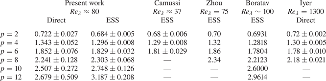
Figure 19(a) shows scaling exponents $\xi _{g}^{p}$ and $\xi _{t}^{p}$ computed using the ESS method, compared to the original predictions by Kolmogorov (Reference Kolmogorov1941, KM41) extended to $p > 3$, the refined similarity hypotheses of Kolmogorov (Reference Kolmogorov1962, KM62), the intermittency $\beta$ model by Frisch, Sulem & Nelkin (Reference Frisch, Sulem and Nelkin1978) and the model by She & Leveque (Reference She and Leveque1994). The transverse scaling exponents $\xi _{t}^{p}$ in figure 19 are obtained by making $\langle (\delta u_{t})^{p}\rangle$ depend on the magnitude of transverse velocity differences for $p = 3$ rather than the longitudinal, thus following the ESS method (Camussi et al. Reference Camussi, Barbagallo, Guj and Stella1996; Grossmann, Lohse & Reeh Reference Grossmann, Lohse and Reeh1997). The refined similarity hypotheses are found to hold, but there is a visible tendency of $\xi _{t}^{p}$ to deviate from the longitudinal scaling for $p \geqslant 4$. This is to be ascribed to the Reynolds number and the residual anisotropy of the flow, as argued by Iyer et al. (Reference Iyer, Sreenivasan and Yeung2017).

Figure 19.

(a) Scaling exponents $\xi _{g}^{p}$ and $\xi _{t}^{p}$ computed with the ESS method versus $p$ for orders up to $20$ ($x = 25$). In the same plot there are the results from different intermittency models assuming $\mu = 0.08$: $\circ$, $\xi _{g}^{p}$; $\ast$, $\xi _{t}^{p}$; solid line, KM41 model; dashed line, KM62 model; dot-dashed line, $\beta$ model; and dotted line, She–Leveque model. (b) Behaviours of the intermittency exponent along $x$ computed according to two different methods: solid line, based on $\langle \epsilon (\boldsymbol {x}+\boldsymbol {r}) \epsilon (\boldsymbol {x}) \rangle /\langle \epsilon \rangle ^{2} \sim (L/r)^{\mu }$; and dotted line, $\mu = 2-\xi _{g}^{6}$.

Figure 19(b) displays the evolution of the intermittency exponent $\mu$ along the streamwise direction; the quantity defined in (3.20) is also employed in the $\beta$-model by Frisch et al. (Reference Frisch, Sulem and Nelkin1978). The $\mu$ exponent is calculated directly from the slope of the correlation coefficient obtained by dividing the autocorrelation of dissipation by $\langle \epsilon \rangle ^{2}$ for separations in the inertial range; see figure 20. A second possible way to obtain $\mu$ is by using the expression relating the longitudinal sixth-order moment to the autocorrelation of dissipation (Frisch et al. Reference Frisch, Sulem and Nelkin1978):

(3.21)\begin{equation} \frac{\langle (\delta u_{g})^{6}\rangle}{r^2} \sim \langle \epsilon(\boldsymbol{x}+\boldsymbol{r}) \epsilon(\boldsymbol{x}) \rangle. \end{equation}

The two quantities are reported in figure 19(b). As the reference value reported in many studies for the intermittency exponent is $\mu = 0.25 \pm 0.05$, which is deemed to be valid for high-Reynolds-number flows (Pope Reference Pope2000), the values calculated here suggest that the effect generated by intermittent structures on small-scale turbulence in the moderate-Reynolds-number range is less intense than at high Reynolds numbers. It is noticed that the method based on sixth-order structure functions, (3.21), displays a decay in the $x$-direction that is not expected nor recovered in the calculation of $\mu$ directly from the definition (3.20).

Figure 20.

Dissipation correlation coefficient at $x=25$: solid line, $\langle \epsilon (\boldsymbol {x}+\boldsymbol {r}) \epsilon (\boldsymbol {x}) \rangle /\langle \epsilon \rangle ^{2}$ as calculated from its definition; and dot-dashed line, $a_{d}(r/\eta )^{d}$, where $a_{d}=1.07$ and $d=-0.082$. The dashed lines delimit the interval used for the power-law fitting procedure, $25\eta < r < 75\eta$, and the dotted lines demarcate the decorrelation scale $\tilde {r}$.

The decorrelation scale $\tilde {r}$ is defined as the length of decorrelation of the instantaneous dissipation $\epsilon$, i.e. the separation scale $r$ where $\langle \epsilon (\boldsymbol {x}+\boldsymbol {r}) \epsilon (\boldsymbol {x}) \rangle / \langle \epsilon \rangle ^{2}$ becomes unitary with a $1\,\%$ error. In figure 21 the development of $\tilde {r}$ along $x$ is compared to that of the integral scale $L$. The decorrelation scale can be considered as a very large length scale, which in homogeneous isotropic turbulence depends on the Reynolds number and also the intermittency characteristics of the flow.

Figure 21.

Streamwise evolution of the decorrelation scale in comparison with the integral scale: solid line, $\tilde {r}$; and dashed line, $L$. For $x=25$, $\tilde {r}/\eta =135$ and $L/\eta =45$.

3.10. Turbulent energy budgets

The equation governing the transport of $\langle k \rangle$ in a statistically steady case can be written in symbols as

(3.22)\begin{equation} - \mathcal{A} = \mathcal{T}_{p} + \mathcal{T}_{t} + \mathcal{D}_{v} + \mathcal{P} - \langle \tilde{\epsilon}\rangle , \end{equation}

where $\mathcal {A}$ is the contribution by mean advection and $\mathcal {T}_{p}$, $\mathcal {T}_{t}$ and $\mathcal {D}_{v}$ represent pressure, turbulent and diffusive transports; $\mathcal {P}$ and $\langle \tilde {\epsilon }\rangle$ stand for the production and pseudo-dissipation rate of turbulent kinetic energy, defined as

(3.23)\begin{equation} \langle \tilde{\epsilon}\rangle = \frac{1}{{\textit{Re}}_{d_p}} \left\langle \frac{\partial u_i}{\partial x_j}\,\frac{\partial u_i}{\partial x_j} \right\rangle. \end{equation}

As the difference $\langle \epsilon \rangle - \langle \tilde {\epsilon } \rangle$ is seldom important (Pope Reference Pope2000), in this section $\langle \epsilon \rangle$ is used.

In grid turbulence cases, where mean velocity gradients are zero and cross-flow directions $y$ and $z$ are homogeneous, the production term vanishes:

(3.24)\begin{equation} \mathcal{P} ={-} \langle u_{i}u_{j} \rangle \frac{\partial \langle U_i \rangle}{\partial x_{j}} = 0. \end{equation}

In addition, for the Reynolds number computed here, the molecular contribution to transport is negligible. The resulting expression for the budget equation (3.22) thus becomes

(3.25)\begin{equation} \underbrace{ \langle U\rangle \frac{\textrm{d} \langle k \rangle}{\textrm{d}\kern0.9pt{x}}}_{-\mathcal{A}} = \underbrace{-\frac{\textrm{d}\langle u p\rangle}{\textrm{d}\kern0.9pt{x}}}_{\mathcal{T}_{p}} \underbrace{-\,\frac{\textrm{d}\langle u k\rangle}{\textrm{d}\kern0.9pt{x}}}_{\mathcal{T}_{t}} - \langle \tilde{\epsilon} \rangle , \end{equation}

where the single terms are distributed along the $x$-axis as depicted in figure 22.

Figure 22.

Turbulent kinetic energy along the streamwise direction in logarithmic plots. In panel (a) budget terms are reported: solid line, $\mathcal {A}$; dot-dashed line, $\mathcal {T}_{p}$; dotted line, $\mathcal {T}_{t}$; and dashed line, $-\langle \tilde {\epsilon } \rangle$. Panel (b) presents turbulent kinetic energy fluxes: solid line, $\langle U \rangle \langle k \rangle$; dot-dashed line, $\langle u p\rangle$; and dotted line, $\langle u k\rangle$. The inset in (a) displays an enlargement of the budget terms in the range $I_d$ in linear scale.

Two regions can be identified in figure 22: a near-field region where the three conservative terms redistribute the kinetic energy along $x$, and a far-field region where pressure and turbulent transports become negligible. Thus dissipation is solely balanced by turbulent kinetic energy advection; see figure 22(a) and its inset. A possible downstream boundary for the near-field region can be set at $x = 2$, where the turbulent and pressure transports become 100 times smaller than advection and dissipation.

The near-field region can be subdivided into two subregions. By considering the ligament diameter $d_f$ as the length scale, a region very close to the metal foam is identified for $x^\ast /d_f < 0.5$, where turbulent transport is larger than the advective one. This region is characterised by the sustainment of turbulence by means of streamwise fluctuations, which is counter-balanced by dissipation, as pressure and advective transports account for negligible shares. The second subregion extends for $0.5 < x^\ast /d_f < 14$, where turbulent kinetic energy is provided through pressure and advective mechanisms while dissipation and turbulent transport drain $\langle k \rangle$; see figure 22(a).

Data gathered by Norberg (Reference Norberg1998) indicate that the vortex formation length $\ell _f$ for the present Reynolds number based on the mean diameter of the filaments, ${\textit {Re}}_{d_f} = 560$, lies in the range $1.5 d_f < \ell _f < 2 d_f$; see Bloor, Gerrard & Lighthill (Reference Bloor, Gerrard and Lighthill1966) for other possible definitions of the vortex formation length. Figure 22(a) displays that this range matches the streamwise location where all the transport terms in (3.25) peak. Therefore, the present data suggest that kinetic energy is originated in the second part of the near-field region, where transport mechanisms show local peaks. Turbulent kinetic energy $\langle k \rangle$ is drained from here by the turbulent transport, which transfers turbulent fluctuations upstream, as indicated by the negative sign of the turbulent flux (see figure 22b), feeding the region very close to the metal foam. On the other hand, pressure and advective mechanisms are found to provide turbulent kinetic energy in the entire region $0.5 < x^\ast /d_f < 14$, and the signs of the relative fluxes indicate that velocity fluctuations are transferred downstream. At the coordinate $x^\ast /d_f=14$ ($x=2$), fluxes $\langle u p\rangle$ and $\langle u k\rangle$ become constant in the streamwise direction, leading to the budget reported in (3.4) for $x>2$, which is typical in developed decaying flows; see figure 22(a) and its inset, which reports the budget terms in the $I_d$ region.

In order to separately assess the behaviour of streamwise and cross-flow velocity fluctuations, the transport equations for velocity variances are analysed. The budget of streamwise velocity variance reads

(3.26)\begin{equation} \underbrace{ \langle U \rangle \frac{\textrm{d} \langle u^{2} \rangle}{\textrm{d}\kern0.9pt{x}}}_{-\mathcal{A}^u} = \underbrace{- \frac{\textrm{d} \langle u^{3} \rangle}{ {\textrm{d}\kern0.9pt{x}}}}_{\mathcal{T}_{t}^u} \underbrace{-\,2\frac{\textrm{d} \langle u p \rangle}{ {\textrm{d}\kern0.9pt{x}}}}_{\mathcal{T}_{p}^u} \underbrace{+\,2\left\langle p \,\frac{\partial u}{\partial x} \right\rangle}_{\mathcal{S}^u} - \langle \widetilde{\epsilon_u} \rangle, \end{equation}

where, from left to right, the first three terms, respectively, represent the advective, turbulent and pressure transports of $\langle u^2 \rangle$, $\langle p \partial u/\partial x \rangle$ is the pressure strain term and $\widetilde {\epsilon _u}$ stands for the $u$-variance pseudo-dissipation rate, $\widetilde {\epsilon _u} = 2 ((\partial u/\partial x_j) \, (\partial u/\partial x_j)) / {\textit {Re}}_{d_p}$. The diffusive transport is again neglected with respect to the other terms. Equations similar to (3.26) can be derived for the transverse velocity components, $v$ and $w$. As the flow is isotropic on $y$–$z$ planes, statistics for the transverse velocity component are obtained by averaging results along $y$ and $z$. For conciseness, the transverse velocity component is indicated by $v$ and its direction by $y$,

(3.27)\begin{equation} \underbrace{ \langle U \rangle \frac{\textrm{d} \langle v^{2} \rangle}{\textrm{d}\kern0.9pt{x}}}_{-\mathcal{A}^v} = \underbrace{- \frac{\textrm{d} \langle u v^{2} \rangle}{ {\textrm{d}\kern0.9pt{x}}}}_{\mathcal{T}_{t}^v} \underbrace{+\,2\left\langle p\, \frac{\partial v}{\partial y} \right\rangle}_{\mathcal{S}^v} - \langle \widetilde{\epsilon_v} \rangle, \end{equation}

where the terms have the same interpretation as in (3.26), and the pseudo-dissipation rate of the $v$-variance is computed as $\widetilde {\epsilon _v} = 2 ((\partial v/\partial x_j) \, (\partial v/\partial x_j)) / {\textit {Re}}_{d_p}$. Note that, with respect to equation (3.25), budgets of velocity component variances include the pressure strain terms. As will be shown in the following, the role of these terms is to redistribute kinetic energy among the velocity components and thus it is responsible for the ‘return to isotropy’ in homogeneous turbulence. Such a phenomenon has been studied for several decades as it is involved in second-order turbulence models; see, for example, the works by Rotta (Reference Rotta1951) and Lumley & Newman (Reference Lumley and Newman1977). Pressure strain terms are not included in (3.25) as their sum $\mathcal {S}^u + 2\mathcal {S}^v$ vanishes because of incompressibility.

Figures 23 and 24 show the velocity variance budgets and fluxes along the streamwise coordinate. It appears that transport mechanisms are more intense in the $\langle u^2\rangle$ budget with respect to $\langle v^2\rangle$, while dissipations $\langle \widetilde {\epsilon _u}\rangle$ and $\langle \widetilde {\epsilon _v}\rangle$ are almost equal. The behaviour of the pressure strain terms reveals that turbulent energy is drained from the streamwise velocity fluctuations, as $\mathcal {S}^u$ represents a sink term in the $\langle u^2\rangle$ budget, and provided to cross-flow velocity fluctuations, where $\mathcal {S}^v$ acts as a source; see figures 23(a) and 24(a). The role of $\mathcal {S}^u$ and $\mathcal {S}^v$ does not change along the whole streamwise extension of the domain, as shown by the insets in figures 23(a) and 24(a). This occurs because, as reported in § 3.2, flow anisotropy is conserved in the flow domain considered. In the decaying region $I_d$, the pressure strain terms maintain an intensity comparable to the advective and dissipation terms, suggesting that the isotropic condition would have been reached in a longer computational domain.

Figure 23.

Variance of streamwise velocity component along the streamwise direction in logarithmic plots. In panel (a) budget terms are reported: solid line, $\mathcal {A}^u$; dotted line, $\mathcal {T}_{t}^u$; dot-dashed line, $\mathcal {T}_{p}^u$; solid line with circles, $\mathcal {S}^u$; and dashed line, $-\langle \widetilde {\epsilon _u} \rangle$. Panel (b) presents $\langle u^2 \rangle$ fluxes: solid line, $\langle U \rangle \langle u^2 \rangle$; dot-dashed line, $\langle u p\rangle$; and dotted line, $\langle u^3\rangle$. The inset in (a) displays an enlargement of the budget terms in the range $I_d$ in linear scale.

Figure 24.

Variance of cross-flow velocity component along the streamwise direction in logarithmic plots. In panel (a) budget terms are reported: solid line, $\mathcal {A}^v$; dotted line, $\mathcal {T}_{t}^v$; solid line with circles, $\mathcal {S}^v$; and dashed line, $-\langle \widetilde {\epsilon _v} \rangle$. Panel (b) presents $\langle v^2 \rangle$ fluxes: solid line, $\langle U \rangle \langle v^2 \rangle$; and dotted line, $\langle uv^2\rangle$. The inset in (a) displays an enlargement of the budget terms in the range $I_d$ in linear scale.

The profiles in figures 23 and 24 show that the $u$-variance terms behave very similarly to the budgets and fluxes of turbulent kinetic energy reported in figure 22. In particular, the peaks of turbulent, advective and pressure transports are located at the same distance from the metal foam, comparable to the vortex formation length. This suggests that velocity fluctuations are more intensely triggered along the streamwise direction with respect to the transverse ones. On the other hand, the $v$-variance terms peak slightly downstream with respect to terms in the $\langle u^2 \rangle$ and $\langle k \rangle$ budgets, and the negative peak of turbulent transport is not very intense (see figure 24a), but it drains enough energy to sustain cross-flow fluctuations in the region just downstream of the metal foam. Another difference with respect to the $\langle u^2 \rangle$ terms is the positive – yet not that intense – turbulent flux very close to the metal foam, indicating that cross-flow fluctuations are more correlated with positive $u$-fluctuations in this region (see figure 24b).