


1. Introduction
Over the past century, the study of rough-wall turbulence continues to challenge researchers, reflecting the profound complexities of this field and its critical implications across a wide range of engineering applications. Central to these investigations is the ongoing challenge of accurately characterising drag as a function of surface properties, particularly at full-scale conditions. While significant progress has been achieved through advancements in experimental and numerical capabilities, key foundational questions remain unanswered, requiring further targeted research (Chung et al. Reference Chung, Hutchins, Schultz and Flack2021).
Predictive frameworks of frictional drag often assume homogeneous surface roughness. However, this assumption fails for surfaces characterised by spanwise topographical heterogeneity, a feature common in many real-world applications. Examples include environmental flows, such as fluvial sediment transport and bedform formation (Chiu & McSparran Reference Chiu and McSparran1966; Colombini Reference Colombini1993; McLelland, Ashworth & Best Reference McLelland, Ashworth and Best1999; Nikora & Roy Reference Nikora and Roy2012; Scherer et al. Reference Scherer, Uhlmann, Kidanemariam and Krayer2022), atmospheric boundary layer flows over wind farms and heterogeneous terrains (Markfort et al. Reference Markfort, Zhang and Porté-Agel2012; Stevens, Gayme & Meneveau Reference Stevens, Gayme and Meneveau2016; Alfredsson & Segalini Reference Alfredsson and Segalini2017; Bossuyt, Meneveau & Meyers Reference Bossuyt, Meneveau and Meyers2018; Medjnoun et al. Reference Medjnoun, Rodriguez-Lopez, Ferreira, Griffiths, Meyers and Ganapathisubramani2021) engineering applications like renewable energy systems and heat exchangers (Barros & Christensen Reference Barros and Christensen2014; Chitrakar, Neopane & Dahlhaug Reference Chitrakar, Neopane and Dahlhaug2016; Pathikonda & Christensen Reference Pathikonda and Christensen2017; Deyn et al. Reference Deyn, Schmidt, Rrlü, Stroh, Kriegseis, Böhm and Frohnapfel2022b
; Wang et al. Reference Wang, Luo, Wang, Cao and Wu2024) as well as marine transportation systems (Monty et al. Reference Monty, Dogan, Hanson, Scardino, Ganapathisubramani and Hutchins2016; Murphy et al. Reference Murphy, Barros, Schultz and Flack2018; Nugroho et al. Reference Nugroho, Monty, Utama, Ganapathisubramani and Hutchins2021; Kaminaris et al. Reference Kaminaris, Balaras, Schultz and Volino2023; Medjnoun et al. Reference Medjnoun, Ferreira, Reinartz, Nugroho, Monty, Hutchins and Ganapathisubramani2023). Under specific conditions, i.e. when the dominant spanwise length scale (spacing, $S$
, or width,
$S$
, or width, $W$
, of the surface) is comparable to the boundary layer thickness (
$W$
, of the surface) is comparable to the boundary layer thickness ( $\delta$
), these surfaces can promote flow channelling (Mejia-Alvarez & Christensen Reference Mejia-Alvarez and Christensen2013), resulting in high-momentum pathways (HMPs) and low-momentum pathways (LMPs). These features are associated with large-scale secondary flows, known as Prandtl’s secondary flows of the second kind, which are critical to understanding the interplay between surface topology and turbulent flow dynamics (Hinze Reference Hinze1973; Anderson et al. Reference Anderson, Barros, Christensen and Awasthi2015; Kevin et al. Reference Kevin, Monty, Bai, Pathikonda, Nugroho, Barros, Christensen and Hutchins2017; Hwang & Lee Reference Hwang and Lee2018; Stroh et al. Reference Stroh, Schä, Forooghi and Frohnapfel2020). At this stage, it is important to note that there are two types of surface heterogeneities. First is strip-type heterogeneity, generated by alternating strips of rough(er)/smooth(er) surfaces, where secondary flows are generated with HMPs over the rough(er) strips and LMPs over the smooth(er) strips. This arrangement is known to change depending on the width of the roughness strip (Nugroho, Hutchins & Monty Reference Nugroho, Hutchins and Monty2013; Barros & Christensen Reference Barros and Christensen2019; Wangsawijaya et al. Reference Wangsawijaya, Baidya, Chung, Marusic and Hutchins2020; Medjnoun et al. Reference Medjnoun, Rodriguez-Lopez, Ferreira, Griffiths, Meyers and Ganapathisubramani2021). Second is ridge-type heterogeneity where secondary flows are generated by adjacent ridges with valleys inbetween. In this case, HMPs are over valleys and LMPs are over the ridges and this arrangement can change depending on the width of the ridge/valley (Vanderwel & Ganapathisubramani Reference Vanderwel and Ganapathisubramani2015; Medjnoun, Vanderwel & Ganapathisubramani Reference Medjnoun, Vanderwel and Ganapathisubramani2018).
$\delta$
), these surfaces can promote flow channelling (Mejia-Alvarez & Christensen Reference Mejia-Alvarez and Christensen2013), resulting in high-momentum pathways (HMPs) and low-momentum pathways (LMPs). These features are associated with large-scale secondary flows, known as Prandtl’s secondary flows of the second kind, which are critical to understanding the interplay between surface topology and turbulent flow dynamics (Hinze Reference Hinze1973; Anderson et al. Reference Anderson, Barros, Christensen and Awasthi2015; Kevin et al. Reference Kevin, Monty, Bai, Pathikonda, Nugroho, Barros, Christensen and Hutchins2017; Hwang & Lee Reference Hwang and Lee2018; Stroh et al. Reference Stroh, Schä, Forooghi and Frohnapfel2020). At this stage, it is important to note that there are two types of surface heterogeneities. First is strip-type heterogeneity, generated by alternating strips of rough(er)/smooth(er) surfaces, where secondary flows are generated with HMPs over the rough(er) strips and LMPs over the smooth(er) strips. This arrangement is known to change depending on the width of the roughness strip (Nugroho, Hutchins & Monty Reference Nugroho, Hutchins and Monty2013; Barros & Christensen Reference Barros and Christensen2019; Wangsawijaya et al. Reference Wangsawijaya, Baidya, Chung, Marusic and Hutchins2020; Medjnoun et al. Reference Medjnoun, Rodriguez-Lopez, Ferreira, Griffiths, Meyers and Ganapathisubramani2021). Second is ridge-type heterogeneity where secondary flows are generated by adjacent ridges with valleys inbetween. In this case, HMPs are over valleys and LMPs are over the ridges and this arrangement can change depending on the width of the ridge/valley (Vanderwel & Ganapathisubramani Reference Vanderwel and Ganapathisubramani2015; Medjnoun, Vanderwel & Ganapathisubramani Reference Medjnoun, Vanderwel and Ganapathisubramani2018).
Despite significant advances, most previous research on secondary flows predominantly focuses on low to moderate Reynolds numbers (Medjnoun et al. Reference Medjnoun, Vanderwel and Ganapathisubramani2018; Nikora et al. Reference Nikora, Stoesser, Cameron, Stewart, Papadopoulos, Ouro, McSherry, Zampiron, Marusic and Falconer2019; Nugroho et al. Reference Nugroho, Monty, Utama, Ganapathisubramani and Hutchins2021; Deyn et al. Reference Deyn, Gatti and Frohnapfel2022a
; Guo et al. Reference Guo, Fang, Zhong and Moulinec2022; Frohnapfel et al. Reference Frohnapfel, von Deyn, Yang, Neuhauser, Stroh, Örlü and Gatti2024). At higher Reynolds numbers, there is an increasing scale separation between near-wall and outer-layer motions and the differences between these layers becomes more pronounced (Smits et al. Reference Smits, McKeon and Marusic2011b
). In a canonical boundary layer, there are several critical coherent structures ranging from near-wall streaks/vortices that are a foundational energy-generating mechanism (Jiménez & Pinelli Reference Jiménez and Pinelli1999) and a hierarchical organisation of attached eddies that grow in size/strength away from the wall (Marusic & Monty Reference Marusic and Monty2019). There is the emergence of large-scale motions (LSMs) (size roughly $3\delta$
) and very large-scale motions (VLSMs) (sometimes also referred to as ‘superstructures’ and size approximately 6
$3\delta$
) and very large-scale motions (VLSMs) (sometimes also referred to as ‘superstructures’ and size approximately 6 $\delta$
) that occupy the log region of flow and act as conveyors of energy and momentum across the boundary layer (Guala, Hommema & Adrian Reference Guala, Hommema and Adrian2006; Marusic, Mathis & Hutchins Reference Marusic, Mathis and Hutchins2010; Smits et al. Reference Smits, McKeon and Marusic2011b
). Moreover, as these larger scales emerge with increasing Reynolds numbers, interactions between them and the near-wall cycle become increasingly significant with larger-scales modulating and amplifying the near-wall region (Hutchins & Marusic Reference Hutchins and Marusic2007a
,
Reference Hutchins and Marusicb
). Introduction of secondary flows through surface heterogeneity at these higher Reynolds numbers could/will affect the naturally occurring structures and this has largely been unexplored.
$\delta$
) that occupy the log region of flow and act as conveyors of energy and momentum across the boundary layer (Guala, Hommema & Adrian Reference Guala, Hommema and Adrian2006; Marusic, Mathis & Hutchins Reference Marusic, Mathis and Hutchins2010; Smits et al. Reference Smits, McKeon and Marusic2011b
). Moreover, as these larger scales emerge with increasing Reynolds numbers, interactions between them and the near-wall cycle become increasingly significant with larger-scales modulating and amplifying the near-wall region (Hutchins & Marusic Reference Hutchins and Marusic2007a
,
Reference Hutchins and Marusicb
). Introduction of secondary flows through surface heterogeneity at these higher Reynolds numbers could/will affect the naturally occurring structures and this has largely been unexplored.
Early insights into the interactions between secondary flows and boundary layer structures emerged from Nugroho et al. (Reference Nugroho, Hutchins and Monty2013), who introduced ‘herringbone’ riblet-patterned surfaces to passively control turbulent boundary layers and perturb the naturally occurring large-scale coherent motions. In retrospect, this is now considered a strip-type heterogeneity and their study revealed substantial modifications in the energy distribution among the largest energetic structures across the boundary layer. Subsequent works on strip-type heterogeneity (Pathikonda & Christensen Reference Pathikonda and Christensen2017; Awasthi & Anderson Reference Awasthi and Anderson2018) examined amplitude and frequency modulation effects for irregular and regular roughness arrangements, respectively. Pathikonda & Christensen (Reference Pathikonda and Christensen2017) reported that roughness enhances amplitude and frequency modulations close to the wall, while Awasthi & Anderson (Reference Awasthi and Anderson2018) demonstrated that a distinct outer peak associated with LSMs, termed ‘modulators’, is preserved within LMPs but vanishes in HMP zones, where turbulent coherent motions exhibit steeper and shorter spatial extents. Additional studies have explored different types of surface heterogeneity and their effects on the spectral and structural attributes of various flows. In their experimental study of a turbulent boundary layer over a ridge-type surface, Medjnoun et al. (Reference Medjnoun, Vanderwel and Ganapathisubramani2018) revealed changes in energy redistribution across all scales, with effects varying according to the spanwise wavelength of the surface heterogeneity. In a direct numerical simulation (DNS) of a fully turbulent pipe flow over three-dimensional wavy topography, Chan et al. (Reference Chan, MacDonald, Chung, Hutchins and Ooi2018) showed that energy is reorganised from the largest to the shorter streamwise wavelengths, with spectral peaks correlated with the characteristic roughness length scale. Using a similar surface roughness to that of Pathikonda & Christensen (Reference Pathikonda and Christensen2017), Barros & Christensen (Reference Barros and Christensen2019) found significant variations in spectral content across the spanwise direction of the surface heterogeneity. More specifically, a shift in energy content to shorter wavelengths above the LMPs, whereas the impact was less pronounced in the HMPs.
More recently, in their studies of open-channel flows, Zampiron, Cameron & Nikora (Reference Zampiron, Cameron and Nikora2020) and Luo et al. (Reference Luo, Stoesser, Cameron, Nikora, Zampiron and Patella2023) demonstrated that for heterogeneous surfaces with spanwise spacings $S/\delta \leqslant 1$
, VLSMs are suppressed, arguing that secondary motions absorb VLSM energy. They also identified a signature of secondary flow instability, manifesting as the meandering of HMPs and LMPs. Similarly, using large-eddy simulations of turbulent flow over a randomly rough surface, Ma et al. (Reference Ma, Xu, Sung and Huang2023) found that secondary motions play a crucial role in redistributing energy, enhancing turbulence intensity in the outer region and modifying spectral peaks. Their results further suggest that roughness-induced secondary motions alter the organisation of coherent structures, leading to deviations from classical outer-layer similarity. Consistent with Zampiron et al. (Reference Zampiron, Cameron and Nikora2020), Wangsawijaya et al. (Reference Wangsawijaya, Baidya, Chung, Marusic and Hutchins2020) observed the meandering behaviour of secondary motions and later characterised their unsteadiness in a strip-type heterogeneous rough-wall boundary layer (Wangsawijaya & Hutchins Reference Wangsawijaya and Hutchins2022). They found that secondary motions and large-scale structures can coexist within certain limits, with maximum secondary flow instabilities occurring at
$S/\delta \leqslant 1$
, VLSMs are suppressed, arguing that secondary motions absorb VLSM energy. They also identified a signature of secondary flow instability, manifesting as the meandering of HMPs and LMPs. Similarly, using large-eddy simulations of turbulent flow over a randomly rough surface, Ma et al. (Reference Ma, Xu, Sung and Huang2023) found that secondary motions play a crucial role in redistributing energy, enhancing turbulence intensity in the outer region and modifying spectral peaks. Their results further suggest that roughness-induced secondary motions alter the organisation of coherent structures, leading to deviations from classical outer-layer similarity. Consistent with Zampiron et al. (Reference Zampiron, Cameron and Nikora2020), Wangsawijaya et al. (Reference Wangsawijaya, Baidya, Chung, Marusic and Hutchins2020) observed the meandering behaviour of secondary motions and later characterised their unsteadiness in a strip-type heterogeneous rough-wall boundary layer (Wangsawijaya & Hutchins Reference Wangsawijaya and Hutchins2022). They found that secondary motions and large-scale structures can coexist within certain limits, with maximum secondary flow instabilities occurring at $S/\delta \sim O(1)$
. More recently, Zhdanov, Jelly & Busse (Reference Zhdanov, Jelly and Busse2024) numerically investigated the influence of ridge-type heterogeneity in turbulent channel flow and reported a significant increase in energy content at higher wavelengths at spanwise locations corresponding to the centres of secondary flows.
$S/\delta \sim O(1)$
. More recently, Zhdanov, Jelly & Busse (Reference Zhdanov, Jelly and Busse2024) numerically investigated the influence of ridge-type heterogeneity in turbulent channel flow and reported a significant increase in energy content at higher wavelengths at spanwise locations corresponding to the centres of secondary flows.
While these studies document the interaction between secondary flows and naturally occurring structures, the friction-based Reynolds number, $\textit{Re}_\tau = \delta U_\tau /\nu$
(where
$\textit{Re}_\tau = \delta U_\tau /\nu$
(where $U_\tau$
is the skin-friction velocity and
$U_\tau$
is the skin-friction velocity and $\nu$
is the kinematic viscosity) of the above-mentioned studies are limited. It is well established that higher Reynolds numbers (
$\nu$
is the kinematic viscosity) of the above-mentioned studies are limited. It is well established that higher Reynolds numbers ( $\textit{Re}_\tau \geqslant 3000)$
are required to clearly observe the presence of VLSMs in streamwise spectra in the outer region. Therefore, it is important to examine the influence of secondary motions on these VLSMs and LSMs at higher Reynolds numbers to understand their interplay. The current study investigates the interaction between ridge-induced secondary flows and turbulent boundary layers at high Reynolds numbers, with specific focus on the interaction between turbulent structures generated by ridges and the naturally occurring energy containing motions. Using an in-house floating-element drag balance (FEDB) for wall-shear stress measurements and hot-wire anemometry (HWA) for spectral analysis, we address some of the gaps in the spectral signature of secondary motions and its coexistence with boundary layer structures over spanwise heterogeneous surfaces across different Reynolds numbers.
$\textit{Re}_\tau \geqslant 3000)$
are required to clearly observe the presence of VLSMs in streamwise spectra in the outer region. Therefore, it is important to examine the influence of secondary motions on these VLSMs and LSMs at higher Reynolds numbers to understand their interplay. The current study investigates the interaction between ridge-induced secondary flows and turbulent boundary layers at high Reynolds numbers, with specific focus on the interaction between turbulent structures generated by ridges and the naturally occurring energy containing motions. Using an in-house floating-element drag balance (FEDB) for wall-shear stress measurements and hot-wire anemometry (HWA) for spectral analysis, we address some of the gaps in the spectral signature of secondary motions and its coexistence with boundary layer structures over spanwise heterogeneous surfaces across different Reynolds numbers.
2. Experimental methods
Experiments were conducted in the newly commissioned boundary layer wind tunnel (BLWT), a closed-return facility at the University of Southampton. This Göttingen-type tunnel has a 12 m-long test section in the $ x$
-direction, with a cross-sectional area of 1 m
$ x$
-direction, with a cross-sectional area of 1 m $\times$
1.2 m in the wall-normal (
$\times$
1.2 m in the wall-normal ( $ y$
-direction) and spanwise (
$ y$
-direction) and spanwise ( $ z$
-direction) directions. The BLWT features a
$ z$
-direction) directions. The BLWT features a $7:1$
contraction in the flow-conditioning section to ensure a uniform inflow profile, with free stream turbulence intensity consistently below 0.1 % within the operational speed range. A cooling unit maintains the air temperature within
$7:1$
contraction in the flow-conditioning section to ensure a uniform inflow profile, with free stream turbulence intensity consistently below 0.1 % within the operational speed range. A cooling unit maintains the air temperature within $\pm 0.1\,^{\circ }\mathrm{C}$
, ensuring stability for temperature-sensitive measurements. This precise temperature control is achieved using two heat exchangers and a PID (proportional integral derivative) temperature controller.
$\pm 0.1\,^{\circ }\mathrm{C}$
, ensuring stability for temperature-sensitive measurements. This precise temperature control is achieved using two heat exchangers and a PID (proportional integral derivative) temperature controller.
Boundary layers develop directly on the wind tunnel floor under a mild favourable pressure gradient ( $K \leqslant 7.5\times 10^{-9}$
) due to the fixed cross-sectional area of the test section. Previous studies have shown that this level of acceleration can be considered as a standard boundary layer (Volino, Schultz & Flack Reference Volino, Schultz and Flack2007). To ensure a laminar-to-turbulent transition, the boundary layer was tripped 50 mm from the leading edge of the test section using a zigzag turbulator tape with a 6 mm point-to-point spacing and a thickness of 0.5 mm. The ridges are installed just downstream from this tripping point. At the measurement location (approximately 8.4 m from the inlet), the floorboard includes a central cutout to accommodate the FEDB. Static-pressure taps were installed around the cutout, approximately 50 mm from its edges, to measure the local streamwise pressure gradient and apply corrections to the FEDB measurements. Note that these corrections are constant across the different cases (and can be considered as a direct current offset due to the mild favourable pressure gradient in the facility). Figure 1 provides a schematic of the BLWT, detailing the experimental methods and surface configurations employed.
$K \leqslant 7.5\times 10^{-9}$
) due to the fixed cross-sectional area of the test section. Previous studies have shown that this level of acceleration can be considered as a standard boundary layer (Volino, Schultz & Flack Reference Volino, Schultz and Flack2007). To ensure a laminar-to-turbulent transition, the boundary layer was tripped 50 mm from the leading edge of the test section using a zigzag turbulator tape with a 6 mm point-to-point spacing and a thickness of 0.5 mm. The ridges are installed just downstream from this tripping point. At the measurement location (approximately 8.4 m from the inlet), the floorboard includes a central cutout to accommodate the FEDB. Static-pressure taps were installed around the cutout, approximately 50 mm from its edges, to measure the local streamwise pressure gradient and apply corrections to the FEDB measurements. Note that these corrections are constant across the different cases (and can be considered as a direct current offset due to the mild favourable pressure gradient in the facility). Figure 1 provides a schematic of the BLWT, detailing the experimental methods and surface configurations employed.
(a) Schematic of the BLWT at the University of Southampton; (b) surface arrangement showing the spanwise-heterogeneous ridge-type surface, including an illustration of the experimental methods. Note that the hot-wire measurements are carried out at just above the peak of the ridge and in the middle of the valley (between adjacent ridges).

2.1. Surface heterogeneity
Surface heterogeneity was introduced by affixing longitudinal triangular ridges to a smooth base. These ridges, modelled on the HS2 configuration by Medjnoun, Vanderwel & Ganapathisubramani (Reference Medjnoun, Vanderwel and Ganapathisubramani2020), are equilateral triangles with a side length of $a = 6.4$
mm and a height of
$a = 6.4$
mm and a height of $h = 5.6$
mm. Three spanwise spacings (
$h = 5.6$
mm. Three spanwise spacings ( $S$
) were tested:
$S$
) were tested: $S = 50$
mm,
$S = 50$
mm, $100$
mm and
$100$
mm and $200$
mm, corresponding to configurations labelled T50, T100 and T200, respectively. These spacings are equivalent to
$200$
mm, corresponding to configurations labelled T50, T100 and T200, respectively. These spacings are equivalent to $S/\delta \approx 0.3, 0.6$
and
$S/\delta \approx 0.3, 0.6$
and $1.3$
, with
$1.3$
, with $h/\delta \approx 4\,\%$
, when scaled with the spanwise-averaged boundary layer thickness
$h/\delta \approx 4\,\%$
, when scaled with the spanwise-averaged boundary layer thickness $\delta$
= 0.15m (which is
$\delta$
= 0.15m (which is $\delta _{99}$
measured as the wall-normal location at which
$\delta _{99}$
measured as the wall-normal location at which $U = 0.99U_\infty$
). We note that this spanwise-averaged value is obtained by only averaging two locations – the peak and valley where we have hot-wire measurements. The difference in
$U = 0.99U_\infty$
). We note that this spanwise-averaged value is obtained by only averaging two locations – the peak and valley where we have hot-wire measurements. The difference in $\delta$
between these two locations is less than 4 % across all cases and Reynolds numbers.
$\delta$
between these two locations is less than 4 % across all cases and Reynolds numbers.
2.2. Drag balance
Wall shear stress was measured using an in-house FEDB designed with a zero-displacement force-feedback system (Aguiar Ferreira, Costa & Ganapathisubramani Reference Aguiar Ferreira, Costa and Ganapathisubramani2024). The floating element, a square of 200 mm side length, was installed flush with the wind tunnel floor, located approximately $60\delta$
from the inlet. The FEDB was subjected to nine free stream velocities (
$60\delta$
from the inlet. The FEDB was subjected to nine free stream velocities ( $U_{\infty }$
) ranging from 10 to 45 m s–1 to determine the frictional drag coefficient
$U_{\infty }$
) ranging from 10 to 45 m s–1 to determine the frictional drag coefficient $C_{\!f} = 2D/(\rho U^2_\infty Ar)$
(where
$C_{\!f} = 2D/(\rho U^2_\infty Ar)$
(where $D$
is the measured drag force and
$D$
is the measured drag force and $Ar$
is the surface area of the balance, which is
$Ar$
is the surface area of the balance, which is $200\times 200\,\rm mm^2$
) as a function of the Reynolds number. Each acquisition lasted 120 s, sampled at 256 Hz, capturing at least 2500 boundary-layer eddy turnover times (
$200\times 200\,\rm mm^2$
) as a function of the Reynolds number. Each acquisition lasted 120 s, sampled at 256 Hz, capturing at least 2500 boundary-layer eddy turnover times ( $\tau _{\textit{eddy}} = \delta /U_{\infty }$
) for the lowest velocity. Five repetitions were conducted at each velocity to ensure statistical significance. Precalibration and postcalibration procedures were performed for each configuration using a standard force transducer. The calibration coefficient varied by less than 0.5 %, ensuring high precision and negligible drift over extended measurements. The overall uncertainty in the skin-friction coefficient (precision and systematic uncertainties) for all the cases was less than
$\tau _{\textit{eddy}} = \delta /U_{\infty }$
) for the lowest velocity. Five repetitions were conducted at each velocity to ensure statistical significance. Precalibration and postcalibration procedures were performed for each configuration using a standard force transducer. The calibration coefficient varied by less than 0.5 %, ensuring high precision and negligible drift over extended measurements. The overall uncertainty in the skin-friction coefficient (precision and systematic uncertainties) for all the cases was less than $\pm 1.5 \,\%$
. A more detailed and comprehensive discussion of the FEDB design, acquisition procedures and measurement uncertainties is available in Aguiar Ferreira et al. (Reference Aguiar Ferreira, Costa and Ganapathisubramani2024). Table 1 shows a list of freestream speeds used to carry out the drag measurements.
$\pm 1.5 \,\%$
. A more detailed and comprehensive discussion of the FEDB design, acquisition procedures and measurement uncertainties is available in Aguiar Ferreira et al. (Reference Aguiar Ferreira, Costa and Ganapathisubramani2024). Table 1 shows a list of freestream speeds used to carry out the drag measurements.
2.3. Hot-wire anemometry
Time-resolved velocity measurements were conducted using two single Auspex A55P05 boundary-layer hot-wire probes. These probes consist of tungsten wires with a diameter of 5 $\unicode{x03BC}$
m and a sensing length of 1 mm, yielding a length-to-diameter ratio of 200, in accordance with the recommendations of Hutchins et al. (Reference Hutchins, Nickels, Marusic and Chong2009). The inner-scaled length of the HWA sensor
$\unicode{x03BC}$
m and a sensing length of 1 mm, yielding a length-to-diameter ratio of 200, in accordance with the recommendations of Hutchins et al. (Reference Hutchins, Nickels, Marusic and Chong2009). The inner-scaled length of the HWA sensor $l^+=lU_{\tau }/\nu$
ranged between 25 and 100 viscous length scales (where
$l^+=lU_{\tau }/\nu$
ranged between 25 and 100 viscous length scales (where $U_\tau = U_\infty \sqrt {C_{\!f}/2}$
). Measurements were recorded simultaneously at two symmetry planes:
$U_\tau = U_\infty \sqrt {C_{\!f}/2}$
). Measurements were recorded simultaneously at two symmetry planes: $z/S = 0$
(valley symmetry plane) and
$z/S = 0$
(valley symmetry plane) and $z/S = 0.5$
(ridge symmetry plane).
$z/S = 0.5$
(ridge symmetry plane).
The set-up was positioned at the same location as the FEDB, and measurements were performed at three free stream velocities: $U_{\infty } \approx 10$
,
$U_{\infty } \approx 10$
, $20$
and
$20$
and $40$
m s−1 as indicated in bold in table 1. A DANTEC StreamLine Pro constant temperature anemometer system was employed, operating at a fixed overheat ratio of 0.8. The wall-normal flow was traversed logarithmically at 50 locations, from
$40$
m s−1 as indicated in bold in table 1. A DANTEC StreamLine Pro constant temperature anemometer system was employed, operating at a fixed overheat ratio of 0.8. The wall-normal flow was traversed logarithmically at 50 locations, from $0.002\delta$
to
$0.002\delta$
to $2\delta$
. Data were recorded for 3–10 min at each position, capturing a minimum of 25 000 boundary layer eddy turnover cycles, sufficient for convergence of turbulence intensity and spectral measurements (Hutchins et al. Reference Hutchins, Nickels, Marusic and Chong2009).
$2\delta$
. Data were recorded for 3–10 min at each position, capturing a minimum of 25 000 boundary layer eddy turnover cycles, sufficient for convergence of turbulence intensity and spectral measurements (Hutchins et al. Reference Hutchins, Nickels, Marusic and Chong2009).
The table shows skin friction coefficient $ C_{\!f} = 2 U^2_\tau /U^2_\infty$
(where
$ C_{\!f} = 2 U^2_\tau /U^2_\infty$
(where $U_\tau$
is the skin-friction velocity), roughness height in inner and outer units (
$U_\tau$
is the skin-friction velocity), roughness height in inner and outer units ( $h^+ = h U_\tau /\nu$
and
$h^+ = h U_\tau /\nu$
and $h/\delta$
) and roughness function
$h/\delta$
) and roughness function $\Delta U^+$
computed using (3.1). The boundary layer thickness for the smooth wall was 0.13
$\Delta U^+$
computed using (3.1). The boundary layer thickness for the smooth wall was 0.13 $m$
and for all heterogeneous surfaces it is 0.15
$m$
and for all heterogeneous surfaces it is 0.15 $m$
(to within 4 % variation across the span). Bold rows indicate HWA measurements.
$m$
(to within 4 % variation across the span). Bold rows indicate HWA measurements.

The raw signal was amplified, low-pass filtered at 30 kHz and sampled at 60 kHz using a 16-bit National Instruments NI-DAQ USB 6212 system. The free stream velocity was monitored using a Pitot-static probe connected to a Furness Controls FCO560 micromanometer. Additionally, a Dantec 90P10 temperature probe measured air temperature, correcting for thermal drift. Precalibration and postcalibration procedures were conducted, and time-based interpolation between calibration coefficients accounted for temperature and electrical drifts, with an overall drift of less than 1 %.
Finally, a note on the way the velocity profiles are non-dimensionalised in this work. For velocity, we use the $U_\tau = U_\infty \sqrt {C_{\!f}/2}$
obtained from the drag balance and therefore is an ‘average’ value across the surface. For inner length scale,
$U_\tau = U_\infty \sqrt {C_{\!f}/2}$
obtained from the drag balance and therefore is an ‘average’ value across the surface. For inner length scale, $\nu /U_\tau$
is used and once again this represents an ‘average’ value. For outer length scale, we use
$\nu /U_\tau$
is used and once again this represents an ‘average’ value. For outer length scale, we use $\delta$
obtained as
$\delta$
obtained as $\delta _{99}$
of a specific profile (either peak or valley). When this is done, we also provide the local
$\delta _{99}$
of a specific profile (either peak or valley). When this is done, we also provide the local $\textit{Re}_\tau = U_\tau \delta /\nu$
for each profile. The differences in
$\textit{Re}_\tau = U_\tau \delta /\nu$
for each profile. The differences in $\textit{Re}_\tau$
between peak and valley are entirely due to the difference in boundary layer thickness between the two spots. As mentioned earlier, the difference in boundary layer thickness is less than 4 %, which manifests in the worst case (for T100 surface) as a 4 % difference in
$\textit{Re}_\tau$
between peak and valley are entirely due to the difference in boundary layer thickness between the two spots. As mentioned earlier, the difference in boundary layer thickness is less than 4 %, which manifests in the worst case (for T100 surface) as a 4 % difference in $\textit{Re}_\tau$
between peak and valley.
$\textit{Re}_\tau$
between peak and valley.
3. Results
This section presents the analysis of results obtained from the FEDB and HWA measurements. Section 3.1 investigates the behaviour of frictional drag at high Reynolds numbers under the influence of spanwise surface heterogeneity. Section 3.2 explores the effects of Reynolds number on flow heterogeneity. Sections 3.4, 3.5 and 3.6 examine the influence of surface heterogeneity and Reynolds number on turbulence intensity, spectral characteristics and the VLSMs, respectively. Finally, we have compared the hot-wire data with DNS data in some of these sections, however, we have also provided all mean and turbulence profiles of the smooth-wall data at different Reynolds numbers from the same facility in Appendix A.
( $a$
) Variation of the skin-friction coefficient as a function of Reynolds number, compared with the smooth-wall baseline and Schlichting power law, and (
$a$
) Variation of the skin-friction coefficient as a function of Reynolds number, compared with the smooth-wall baseline and Schlichting power law, and ( $b$
) the associated roughness function computed using (3.1). The blue dashed line represents the classical ‘homogeneous’ fully rough regime, with a
$b$
) the associated roughness function computed using (3.1). The blue dashed line represents the classical ‘homogeneous’ fully rough regime, with a $1/\kappa = 1/0.39$
slope.
$1/\kappa = 1/0.39$
slope.

3.1. Frictional drag
The results from the FEDB are illustrated in figure 2, depicting the response of the wall shear stress to changes in the spanwise spacings of the surface heterogeneity. Figure 2( $a$
) illustrates the variation of the skin-friction coefficient
$a$
) illustrates the variation of the skin-friction coefficient $C_{\kern-1.5pt f}$
as a function of
$C_{\kern-1.5pt f}$
as a function of $\textit{Re}_{x}$
. At low Reynolds numbers, the smooth wall data is consistent with other studies in the literature (but not necessarily with Schlichting’s correlation) and this is presented in our previous work of Aguiar Ferreira et al. (Reference Aguiar Ferreira, Costa and Ganapathisubramani2024). The data also suggests all three surfaces have higher
$\textit{Re}_{x}$
. At low Reynolds numbers, the smooth wall data is consistent with other studies in the literature (but not necessarily with Schlichting’s correlation) and this is presented in our previous work of Aguiar Ferreira et al. (Reference Aguiar Ferreira, Costa and Ganapathisubramani2024). The data also suggests all three surfaces have higher $C_{\!f}$
compared with a smooth wall and this is in line with the increased wetted area of the surfaces with ridges (i.e. two sides of the triangles increase the wetted area). For T50, T100 and T200, there is an increase in wetted area of 16 %, 10 % and 6.5 %, respectively. However, at lower Reynolds number, the
$C_{\!f}$
compared with a smooth wall and this is in line with the increased wetted area of the surfaces with ridges (i.e. two sides of the triangles increase the wetted area). For T50, T100 and T200, there is an increase in wetted area of 16 %, 10 % and 6.5 %, respectively. However, at lower Reynolds number, the $C_{\!f}$
does not necessarily just follow this increased wetted area trend. The T100 surface exhibits the largest
$C_{\!f}$
does not necessarily just follow this increased wetted area trend. The T100 surface exhibits the largest $C_{\!f}$
at lowest Reynolds number. The reasons for this are unclear, but we speculate that this could be due to the viscous boundary layers growing on the sides of the ridges having a greater proportional contribution to
$C_{\!f}$
at lowest Reynolds number. The reasons for this are unclear, but we speculate that this could be due to the viscous boundary layers growing on the sides of the ridges having a greater proportional contribution to $C_{\!f}$
compared with the T200 case (this is consistent with larger wetted area). However, for the T50 case, the boundary layers on the two sides of the triangle could be constrained by the relatively smaller spacing between adjacent ridges. As
$C_{\!f}$
compared with the T200 case (this is consistent with larger wetted area). However, for the T50 case, the boundary layers on the two sides of the triangle could be constrained by the relatively smaller spacing between adjacent ridges. As $\textit{Re}_{x}$
increases, a proportional difference begins to manifest (around
$\textit{Re}_{x}$
increases, a proportional difference begins to manifest (around $\textit{Re}_{x} \approx 10^7$
) with
$\textit{Re}_{x} \approx 10^7$
) with $C_{\!f}$
trends starting to follow the trends in wetted area. The T200 surfaces shows a noticeable reduction in magnitude compared with T50 and T100. At the highest Reynolds number measured (approximately
$C_{\!f}$
trends starting to follow the trends in wetted area. The T200 surfaces shows a noticeable reduction in magnitude compared with T50 and T100. At the highest Reynolds number measured (approximately $\textit{Re}_{x} \approx 3 \times 10^7$
), T50 exhibits the highest frictional drag, followed by T100 and then T200. Regardless of the spanwise spacing between ridges, the
$\textit{Re}_{x} \approx 3 \times 10^7$
), T50 exhibits the highest frictional drag, followed by T100 and then T200. Regardless of the spanwise spacing between ridges, the $C_{\!f}$
remains higher than that of the smooth wall with T50 surface exhibiting a
$C_{\!f}$
remains higher than that of the smooth wall with T50 surface exhibiting a $C_{\!f}$
that is 25 % higher than the smooth wall at the highest
$C_{\!f}$
that is 25 % higher than the smooth wall at the highest $\textit{Re}_{x}$
.
$\textit{Re}_{x}$
.
Figure 2( $a$
) also reveals differences in the decay rate of
$a$
) also reveals differences in the decay rate of $C_{\kern-1.5pt f}$
across cases. The skin-friction coefficient for T50 appears to reach an onset of an asymptote at high
$C_{\kern-1.5pt f}$
across cases. The skin-friction coefficient for T50 appears to reach an onset of an asymptote at high $\textit{Re}_{x}$
, as seen in the nearly constant values at the last measurement points. In contrast, T200 decays similarly to the smooth wall flow but maintains a relatively constant offset from the smooth wall. This suggests that
$\textit{Re}_{x}$
, as seen in the nearly constant values at the last measurement points. In contrast, T200 decays similarly to the smooth wall flow but maintains a relatively constant offset from the smooth wall. This suggests that $C_{\!f}$
may tend towards a constant value at a lower Reynolds number for smaller wavelengths while we certainly need to go to higher Reynolds numbers for larger wavelengths. Together, these trends provide some indications of an envelope of expected
$C_{\!f}$
may tend towards a constant value at a lower Reynolds number for smaller wavelengths while we certainly need to go to higher Reynolds numbers for larger wavelengths. Together, these trends provide some indications of an envelope of expected $C_{\!f}$
for a given geometry, varying between homogeneous-rough-like behaviour for smaller wavelengths and homogeneous-smooth-like trend (but with an offset) for large wavelengths.
$C_{\!f}$
for a given geometry, varying between homogeneous-rough-like behaviour for smaller wavelengths and homogeneous-smooth-like trend (but with an offset) for large wavelengths.
The $C_{\!f}$
of ridge-type and smooth surfaces can be used to quantify the roughness function
$C_{\!f}$
of ridge-type and smooth surfaces can be used to quantify the roughness function $\Delta U^+$
at a given value of
$\Delta U^+$
at a given value of $\textit{Re}_x$
following the work of Medjnoun et al. (Reference Medjnoun, Ferreira, Reinartz, Nugroho, Monty, Hutchins and Ganapathisubramani2023). Assuming that the wake strength parameter
$\textit{Re}_x$
following the work of Medjnoun et al. (Reference Medjnoun, Ferreira, Reinartz, Nugroho, Monty, Hutchins and Ganapathisubramani2023). Assuming that the wake strength parameter $\varPi$
is invariant with Reynolds number and across flow conditions (i.e. assuming outer-layer similarity), the roughness function can be derived using the log and defect formulations of the mean velocity as
$\varPi$
is invariant with Reynolds number and across flow conditions (i.e. assuming outer-layer similarity), the roughness function can be derived using the log and defect formulations of the mean velocity as
 \begin{equation} \Delta U^+ = \sqrt {\frac {2}{C^{S}_{\!f}}} - \sqrt {\frac {2}{C^{R}_{\!f}}} + \frac {1}{\kappa }\ln\!\left (\frac {{\textit{Re}}^R_\tau }{{\textit{Re}}^S_\tau }\right )\!. \end{equation}
Here, $C_{\!f}^S$
and
$C_{\!f}^S$
and $C^R_{\!f}$
are the skin-friction coefficients of smooth and rough surfaces,
$C^R_{\!f}$
are the skin-friction coefficients of smooth and rough surfaces, ${\textit{Re}}^R_\tau = \delta ^R U^R_\tau /\nu$
and
${\textit{Re}}^R_\tau = \delta ^R U^R_\tau /\nu$
and ${\textit{Re}}^S_\tau = \delta ^S U^S_\tau /\nu$
are the skin-friction based Reynolds number of the rough and smooth wall at a given free stream speed (
${\textit{Re}}^S_\tau = \delta ^S U^S_\tau /\nu$
are the skin-friction based Reynolds number of the rough and smooth wall at a given free stream speed ( $U_\infty$
). The third term, which has
$U_\infty$
). The third term, which has ${\textit{Re}}^R_\tau /{\textit{Re}}^S_\tau$
is equal to unity at matched
${\textit{Re}}^R_\tau /{\textit{Re}}^S_\tau$
is equal to unity at matched $\textit{Re}_\tau$
conditions, but, here it makes a small contribution to
$\textit{Re}_\tau$
conditions, but, here it makes a small contribution to $\Delta U^+$
(up to a maximum of 10 % of the final value) depending on the differences in
$\Delta U^+$
(up to a maximum of 10 % of the final value) depending on the differences in $\textit{Re}_\tau$
between smooth and rough walls. We note that this estimation of
$\textit{Re}_\tau$
between smooth and rough walls. We note that this estimation of $\Delta U^+$
is not necessarily correct since the flow does not follow outer-layer similarity (as seen later), but, this provides a way to quantify the overall effect of these heterogeneous surfaces. Therefore, as long as
$\Delta U^+$
is not necessarily correct since the flow does not follow outer-layer similarity (as seen later), but, this provides a way to quantify the overall effect of these heterogeneous surfaces. Therefore, as long as $\textit{Re}_\tau$
values of the smooth and rough-walls are known at a given free stream speed, we can estimate the value of
$\textit{Re}_\tau$
values of the smooth and rough-walls are known at a given free stream speed, we can estimate the value of $\Delta U^+$
for that value of
$\Delta U^+$
for that value of $U_\infty$
and associate that with the corresponding value of
$U_\infty$
and associate that with the corresponding value of $h^+$
. This is similar to the way other studies in internal flows (Deyn et al. Reference Deyn, Gatti and Frohnapfel2022a
; Frohnapfel et al. Reference Frohnapfel, von Deyn, Yang, Neuhauser, Stroh, Örlü and Gatti2024) have estimated
$h^+$
. This is similar to the way other studies in internal flows (Deyn et al. Reference Deyn, Gatti and Frohnapfel2022a
; Frohnapfel et al. Reference Frohnapfel, von Deyn, Yang, Neuhauser, Stroh, Örlü and Gatti2024) have estimated $\Delta U^+$
at matched bulk Reynolds number of channel/pipe flows (using pressure-drop measurements rather than drag balance) to get a general idea about the flow even though the flow does not follow outer similarity.
$\Delta U^+$
at matched bulk Reynolds number of channel/pipe flows (using pressure-drop measurements rather than drag balance) to get a general idea about the flow even though the flow does not follow outer similarity.
Figure 2( $b$
) shows the results of the roughness function versus
$b$
) shows the results of the roughness function versus $h^+$
(inner-scaled ridge height). The values of
$h^+$
(inner-scaled ridge height). The values of $\Delta U^+$
remain relatively low, ranging from 2 to 4 at the highest Reynolds numbers, which is significantly lower than typical rough-wall flows at equivalent Reynolds numbers (Schultz & Flack Reference Schultz and Flack2007; Castro, Segalini & Alfredsson Reference Castro, Segalini and Alfredsson2013; Flack & Schultz Reference Flack and Schultz2014; Squire et al. Reference Squire, Morrill-Winter, Hutchins, Schultz, Klewicki and Marusic2016; Medjnoun et al. Reference Medjnoun, Ferreira, Reinartz, Nugroho, Monty, Hutchins and Ganapathisubramani2023). It is well-established that Reynolds number invariance in
$\Delta U^+$
remain relatively low, ranging from 2 to 4 at the highest Reynolds numbers, which is significantly lower than typical rough-wall flows at equivalent Reynolds numbers (Schultz & Flack Reference Schultz and Flack2007; Castro, Segalini & Alfredsson Reference Castro, Segalini and Alfredsson2013; Flack & Schultz Reference Flack and Schultz2014; Squire et al. Reference Squire, Morrill-Winter, Hutchins, Schultz, Klewicki and Marusic2016; Medjnoun et al. Reference Medjnoun, Ferreira, Reinartz, Nugroho, Monty, Hutchins and Ganapathisubramani2023). It is well-established that Reynolds number invariance in $C_{\kern-1.5pt f}$
primarily arises from pressure drag contributions, which dominate at sufficiently high Reynolds numbers, leading to the fully rough regime (Napoli, Armenio & De Marchis Reference Napoli, Armenio and De Marchis2008; Yuan & Piomelli Reference Yuan and Piomelli2014). However, such contributions require wake-producing roughness features (i.e. streamwise flow separation), which are absent in these spanwise heterogeneous surfaces. Therefore, the low
$C_{\kern-1.5pt f}$
primarily arises from pressure drag contributions, which dominate at sufficiently high Reynolds numbers, leading to the fully rough regime (Napoli, Armenio & De Marchis Reference Napoli, Armenio and De Marchis2008; Yuan & Piomelli Reference Yuan and Piomelli2014). However, such contributions require wake-producing roughness features (i.e. streamwise flow separation), which are absent in these spanwise heterogeneous surfaces. Therefore, the low $\Delta U^+$
values corroborate the absence of pressure-drag-producing roughness elements. This observation aligns with recent studies that report similar trends in heterogeneous surfaces lacking wake-producing roughness features or exhibiting only weak wake formation (Medjnoun et al. Reference Medjnoun, Vanderwel and Ganapathisubramani2018, Reference Medjnoun, Vanderwel and Ganapathisubramani2020; Nugroho et al. Reference Nugroho, Monty, Utama, Ganapathisubramani and Hutchins2021; Deyn et al. Reference Deyn, Gatti and Frohnapfel2022a
; Frohnapfel et al. Reference Frohnapfel, von Deyn, Yang, Neuhauser, Stroh, Örlü and Gatti2024).
$\Delta U^+$
values corroborate the absence of pressure-drag-producing roughness elements. This observation aligns with recent studies that report similar trends in heterogeneous surfaces lacking wake-producing roughness features or exhibiting only weak wake formation (Medjnoun et al. Reference Medjnoun, Vanderwel and Ganapathisubramani2018, Reference Medjnoun, Vanderwel and Ganapathisubramani2020; Nugroho et al. Reference Nugroho, Monty, Utama, Ganapathisubramani and Hutchins2021; Deyn et al. Reference Deyn, Gatti and Frohnapfel2022a
; Frohnapfel et al. Reference Frohnapfel, von Deyn, Yang, Neuhauser, Stroh, Örlü and Gatti2024).
Despite the low magnitude of $\Delta U^+$
, the variation of
$\Delta U^+$
, the variation of $\Delta U^+(h^+)$
for T50 (and to a lesser extent, T100) approaches the
$\Delta U^+(h^+)$
for T50 (and to a lesser extent, T100) approaches the $1/\kappa$
asymptote, suggesting the possible emergence of an aerodynamic roughness length scale (
$1/\kappa$
asymptote, suggesting the possible emergence of an aerodynamic roughness length scale ( $h_{s}$
) at either higher Reynolds numbers or smaller spanwise wavelengths (i.e.
$h_{s}$
) at either higher Reynolds numbers or smaller spanwise wavelengths (i.e. $S$
-scale surfaces). In contrast, for larger wavelengths (T200),
$S$
-scale surfaces). In contrast, for larger wavelengths (T200), $\Delta U^+$
remains invariant with
$\Delta U^+$
remains invariant with $h^+$
, consistent with figure 2(
$h^+$
, consistent with figure 2( $a$
). These results indicate that frictional drag for smooth spanwise heterogeneous surfaces follows two asymptotic limits, a bounded envelope between rough-like and smooth-wall-like behaviours, depending on the relative scale of
$a$
). These results indicate that frictional drag for smooth spanwise heterogeneous surfaces follows two asymptotic limits, a bounded envelope between rough-like and smooth-wall-like behaviours, depending on the relative scale of $S$
to
$S$
to $\delta$
. When
$\delta$
. When $S/\delta \ll 1$
, flow heterogeneity and secondary flow significance depend on
$S/\delta \ll 1$
, flow heterogeneity and secondary flow significance depend on $S$
, and the roughness function exhibits
$S$
, and the roughness function exhibits $k$
-type behaviour for small spanwise wavelengths. Conversely, when
$k$
-type behaviour for small spanwise wavelengths. Conversely, when $S/\delta \geqslant 1$
, flow heterogeneity is primarily governed by
$S/\delta \geqslant 1$
, flow heterogeneity is primarily governed by $\delta$
, with behaviour asymptoting towards the smooth-wall regime as spanwise wavelengths increase.
$\delta$
, with behaviour asymptoting towards the smooth-wall regime as spanwise wavelengths increase.
These findings suggest that secondary flows generated by these surfaces could play a crucial role in redistributing momentum and energy across the turbulent boundary layer. It is important to note that these results are currently applicable only to smooth spanwise heterogeneous surfaces. Further investigation is required to understand the behaviour of pressure-drag-producing spanwise heterogeneous surfaces, which are expected to behave differently, as recently demonstrated by Medjnoun et al. (Reference Medjnoun, Rodriguez-Lopez, Ferreira, Griffiths, Meyers and Ganapathisubramani2021) and Frohnapfel et al. (Reference Frohnapfel, von Deyn, Yang, Neuhauser, Stroh, Örlü and Gatti2024).
3.2. Flow heterogeneity
To assess the effect of surface condition on turbulent boundary layer flow heterogeneity, both the ridge (red) and valley (blue) symmetry planes ( $z/S = 0, 0.5$
) are illustrated in figure 3. The mean streamwise velocity (
$z/S = 0, 0.5$
) are illustrated in figure 3. The mean streamwise velocity ( $U^+$
) and turbulence intensity (
$U^+$
) and turbulence intensity ( $\overline {uu}^+$
) profiles are normalised by the spanwise wavelength-averaged friction velocity
$\overline {uu}^+$
) profiles are normalised by the spanwise wavelength-averaged friction velocity $U_{\tau }$
, measured using the FEDB. The turbulence variance profiles have been corrected for attenuation due to unresolved contributions in the streamwise stress, following Smits et al. (Reference Smits, Monty, Hultmark, Bailey, Hutchins and Marusic2011a
).
$U_{\tau }$
, measured using the FEDB. The turbulence variance profiles have been corrected for attenuation due to unresolved contributions in the streamwise stress, following Smits et al. (Reference Smits, Monty, Hultmark, Bailey, Hutchins and Marusic2011a
).
Figure 3 presents results for the T50 case at low ( $\textit{Re}_\tau \approx 3500$
) and high (
$\textit{Re}_\tau \approx 3500$
) and high ( $\textit{Re}_\tau \approx 12\,500$
) Reynolds numbers, with similar trends observed across other cases. Using area-averaged friction velocity for normalisation, the profiles reveal a horizontal shift due to the ridge height (
$\textit{Re}_\tau \approx 12\,500$
) Reynolds numbers, with similar trends observed across other cases. Using area-averaged friction velocity for normalisation, the profiles reveal a horizontal shift due to the ridge height ( $h^+$
), with the ridge profile shifted towards higher
$h^+$
), with the ridge profile shifted towards higher $y^+$
compared with the valley. This horizontal offset is accompanied by a relatively small vertical shift in
$y^+$
compared with the valley. This horizontal offset is accompanied by a relatively small vertical shift in $U^+$
but a pronounced difference in
$U^+$
but a pronounced difference in $\overline {uu}^+$
.
$\overline {uu}^+$
.
The valley (blue) profiles exhibit higher $U^+$
, corresponding to HMPs, while the ridges (red) form LMPs. This behaviour aligns with previous studies that examined ridge-type spanwise heterogeneous surfaces (Nezu, Tominaga & Nakagawa Reference Nezu, Tominaga and Nakagawa1993; Wang & Cheng Reference Wang and Cheng2006; Vanderwel & Ganapathisubramani Reference Vanderwel and Ganapathisubramani2015; Hwang & Lee Reference Hwang and Lee2018; Castro et al. Reference Castro, Kim, Stroh and Lim2021; Zhdanov et al. Reference Zhdanov, Jelly and Busse2024). The turbulence intensity is redistributed, with LMPs exhibiting elevated
$U^+$
, corresponding to HMPs, while the ridges (red) form LMPs. This behaviour aligns with previous studies that examined ridge-type spanwise heterogeneous surfaces (Nezu, Tominaga & Nakagawa Reference Nezu, Tominaga and Nakagawa1993; Wang & Cheng Reference Wang and Cheng2006; Vanderwel & Ganapathisubramani Reference Vanderwel and Ganapathisubramani2015; Hwang & Lee Reference Hwang and Lee2018; Castro et al. Reference Castro, Kim, Stroh and Lim2021; Zhdanov et al. Reference Zhdanov, Jelly and Busse2024). The turbulence intensity is redistributed, with LMPs exhibiting elevated $\overline {uu}^+$
, while HMPs show reduced turbulence. These observations indicate that large-scale secondary motions could redistribute energy towards ridges through sustained upwash and downwash mechanisms (Anderson et al. Reference Anderson, Barros, Christensen and Awasthi2015).
$\overline {uu}^+$
, while HMPs show reduced turbulence. These observations indicate that large-scale secondary motions could redistribute energy towards ridges through sustained upwash and downwash mechanisms (Anderson et al. Reference Anderson, Barros, Christensen and Awasthi2015).
Inner-scaled mean streamwise velocity and variance profiles above the ridge (red) and valley (blue) at ( $a$
) low and (
$a$
) low and ( $b$
) high Reynolds number for the T50 case. The log-law slope (solid black line) is represented with constants taken as 0.39 and 4.3 for
$b$
) high Reynolds number for the T50 case. The log-law slope (solid black line) is represented with constants taken as 0.39 and 4.3 for $\kappa$
and
$\kappa$
and $B$
, respectively. The vertical solid line shows the inner-normalised ridge height (
$B$
, respectively. The vertical solid line shows the inner-normalised ridge height ( $y^+=h^+$
) whereas the vertical dashed line (
$y^+=h^+$
) whereas the vertical dashed line ( $y^+=l^+$
) represents the wall-normal extent of the spanwise mean and turbulence flow heterogeneity, i.e. the height at which the
$y^+=l^+$
) represents the wall-normal extent of the spanwise mean and turbulence flow heterogeneity, i.e. the height at which the $U^+_{v\textit{alley}}=U^+_{\textit{ridge}}$
and
$U^+_{v\textit{alley}}=U^+_{\textit{ridge}}$
and $\overline {uu}^+_{v\textit{alley}}=\overline {uu}^+_{\textit{ridge}}$
.
$\overline {uu}^+_{v\textit{alley}}=\overline {uu}^+_{\textit{ridge}}$
.

Variation of the wall-normal extent of the turbulence heterogeneity normalised in ( $a$
) inner and (
$a$
) inner and ( $b$
) outer units, as a function of the inner-normalised ridge height, for the different cases and Reynolds numbers. Legend:
$b$
) outer units, as a function of the inner-normalised ridge height, for the different cases and Reynolds numbers. Legend: ![]() - T50;
- T50; ![]() - T100;
- T100; ![]() - T200.
- T200.

At high Reynolds numbers, the turbulence variance profiles reveal additional energetic regions. Specifically, the ridge profile shows a second energetic plateau near $y^+ \approx 1000$
, suggesting strong interactions between secondary flows and outer-layer turbulence. This plateau marks a significant departure from low Reynolds number behaviour, where turbulence is primarily confined near the wall. Farther from the wall, both
$y^+ \approx 1000$
, suggesting strong interactions between secondary flows and outer-layer turbulence. This plateau marks a significant departure from low Reynolds number behaviour, where turbulence is primarily confined near the wall. Farther from the wall, both $U^+$
and
$U^+$
and $\overline {uu}^+$
profiles collapse and asymptote towards
$\overline {uu}^+$
profiles collapse and asymptote towards $U_\infty ^+$
and
$U_\infty ^+$
and $0$
, respectively. This merging point, denoted
$0$
, respectively. This merging point, denoted $l^+$
, represents the height at which spanwise homogeneity is restored, marking the extent of secondary flow influence. This location can also be interpreted as the recovery of similarity in the mean profile.
$l^+$
, represents the height at which spanwise homogeneity is restored, marking the extent of secondary flow influence. This location can also be interpreted as the recovery of similarity in the mean profile.
Figure 4 further examines the scaling of $l^+$
with
$l^+$
with $h^+$
in inner units (figure 4
$h^+$
in inner units (figure 4 $a$
) and with
$a$
) and with $\delta$
in outer units (figure 4
$\delta$
in outer units (figure 4 $b$
). The results reveal a linear relationship between
$b$
). The results reveal a linear relationship between $l^+$
and
$l^+$
and $h^+$
in log–log scaling, indicating a strong but expected dependence of flow heterogeneity on local geometry. However, when scaled by
$h^+$
in log–log scaling, indicating a strong but expected dependence of flow heterogeneity on local geometry. However, when scaled by $\delta$
, the rate of change in
$\delta$
, the rate of change in $l/\delta$
with
$l/\delta$
with $h^+$
is much smaller. This indicates that the spatial significance of secondary motions is governed more by the spanwise characteristic length scale of the surface (
$h^+$
is much smaller. This indicates that the spatial significance of secondary motions is governed more by the spanwise characteristic length scale of the surface ( $S/\delta$
) rather than the Reynolds number (Vanderwel & Ganapathisubramani Reference Vanderwel and Ganapathisubramani2015; Stroh et al. Reference Stroh, Hasegawa, Kriegseis and Frohnapfel2016; Yang & Anderson Reference Yang and Anderson2017; Chung, Monty & Hutchins Reference Chung, Monty and Hutchins2018; Hwang & Lee Reference Hwang and Lee2018; Nikora et al. Reference Nikora, Stoesser, Cameron, Stewart, Papadopoulos, Ouro, McSherry, Zampiron, Marusic and Falconer2019; Wangsawijaya et al. Reference Wangsawijaya, Baidya, Chung, Marusic and Hutchins2020; Zampino, Lasagna & Ganapathisubramani Reference Zampino, Lasagna and Ganapathisubramani2023; Zhdanov et al. Reference Zhdanov, Jelly and Busse2024). This finding highlights a dual impact:
$S/\delta$
) rather than the Reynolds number (Vanderwel & Ganapathisubramani Reference Vanderwel and Ganapathisubramani2015; Stroh et al. Reference Stroh, Hasegawa, Kriegseis and Frohnapfel2016; Yang & Anderson Reference Yang and Anderson2017; Chung, Monty & Hutchins Reference Chung, Monty and Hutchins2018; Hwang & Lee Reference Hwang and Lee2018; Nikora et al. Reference Nikora, Stoesser, Cameron, Stewart, Papadopoulos, Ouro, McSherry, Zampiron, Marusic and Falconer2019; Wangsawijaya et al. Reference Wangsawijaya, Baidya, Chung, Marusic and Hutchins2020; Zampino, Lasagna & Ganapathisubramani Reference Zampino, Lasagna and Ganapathisubramani2023; Zhdanov et al. Reference Zhdanov, Jelly and Busse2024). This finding highlights a dual impact: $(\rm i)$
the localised influence of secondary flows near the surface, and
$(\rm i)$
the localised influence of secondary flows near the surface, and $(\rm ii)$
their interaction with outer-layer dynamics at larger spanwise wavelengths. Finally, it should be noted that the larger values of
$(\rm ii)$
their interaction with outer-layer dynamics at larger spanwise wavelengths. Finally, it should be noted that the larger values of $l/\delta$
in figure 4(b) is indicative of lack of outer-layer similarity, especially for T100 and T200 cases. The differences in collapse between the profiles in peak and valley suggests that we cannot really use these profiles to determine
$l/\delta$
in figure 4(b) is indicative of lack of outer-layer similarity, especially for T100 and T200 cases. The differences in collapse between the profiles in peak and valley suggests that we cannot really use these profiles to determine $\Delta U^+$
to represent the surface (or determine skin-friction). We would need several profiles across the span, compute a spanwise-average, confirm validity of outer-layer similarity and then compute the roughness function.
$\Delta U^+$
to represent the surface (or determine skin-friction). We would need several profiles across the span, compute a spanwise-average, confirm validity of outer-layer similarity and then compute the roughness function.
3.3. A note on wall-normal origin: global versus local $(a, b)$
Wall-normal distributions of the mean streamwise velocity and variance profiles scaled in inner units and
$(a, b)$
Wall-normal distributions of the mean streamwise velocity and variance profiles scaled in inner units and $(c, d)$
their associated one-dimensional premultiplied energy spectra,
$(c, d)$
their associated one-dimensional premultiplied energy spectra, $k_{x}\varPhi _{xx}/U_{\tau }^2$
. Panels (a) and (c) use a global origin (
$k_{x}\varPhi _{xx}/U_{\tau }^2$
. Panels (a) and (c) use a global origin ( $y^+_0 = 0$
at the valley), while (b) and (d) use a local origin (
$y^+_0 = 0$
at the valley), while (b) and (d) use a local origin ( $y^+_0 = h^+$
at the ridge tip). Results represent the T100 case at
$y^+_0 = h^+$
at the ridge tip). Results represent the T100 case at $\textit{Re}_\tau \approx 7400$
. Vertical dashed lines indicate the wall-normal extent of distinct energetic features caused by secondary flows.
$\textit{Re}_\tau \approx 7400$
. Vertical dashed lines indicate the wall-normal extent of distinct energetic features caused by secondary flows.

Before further examining the impact of surface heterogeneity and secondary flows on turbulence properties, a note on the definition of the wall-normal origin is necessary. Figure 5 illustrates the inner-normalised profiles of the mean streamwise velocity and turbulence intensity, along with a contour map of the premultiplied energy spectra, $k_{x}\varPhi _{xx}/U_{\tau }^2$
. Taylor’s ‘frozen turbulence’ hypothesis was applied to transform the spectra from frequency to wavenumber space, where
$k_{x}\varPhi _{xx}/U_{\tau }^2$
. Taylor’s ‘frozen turbulence’ hypothesis was applied to transform the spectra from frequency to wavenumber space, where $k_x = 2\pi /\lambda _x$
represents the streamwise wavenumber, and
$k_x = 2\pi /\lambda _x$
represents the streamwise wavenumber, and $\lambda _x = U/ f$
is its associated wavelength, where
$\lambda _x = U/ f$
is its associated wavelength, where $U$
is the mean streamwise velocity at a given wall-normal location and
$U$
is the mean streamwise velocity at a given wall-normal location and $f$
being the frequency. The choice of
$f$
being the frequency. The choice of $U$
as the convection velocity introduces some uncertainty into the estimated length scales, as the true convection velocity is scale-dependent (Dennis & Nickels Reference Dennis and Nickels2008; Squire et al. Reference Squire, Hutchins, Morrill-Winter, Schultz, Klewicki and Marusic2017). Nevertheless, using a constant convection velocity is consistent with previous experimental studies (Hutchins & Marusic Reference Hutchins and Marusic2007a
; Monty et al. Reference Monty, Hutchins, Ng, Marusic and Chong2009; Squire et al. Reference Squire, Morrill-Winter, Hutchins, Schultz, Klewicki and Marusic2016), enabling direct comparisons with earlier findings. The results in figure 5
$U$
as the convection velocity introduces some uncertainty into the estimated length scales, as the true convection velocity is scale-dependent (Dennis & Nickels Reference Dennis and Nickels2008; Squire et al. Reference Squire, Hutchins, Morrill-Winter, Schultz, Klewicki and Marusic2017). Nevertheless, using a constant convection velocity is consistent with previous experimental studies (Hutchins & Marusic Reference Hutchins and Marusic2007a
; Monty et al. Reference Monty, Hutchins, Ng, Marusic and Chong2009; Squire et al. Reference Squire, Morrill-Winter, Hutchins, Schultz, Klewicki and Marusic2016), enabling direct comparisons with earlier findings. The results in figure 5 $(a{,}b)$
are scaled using a global origin (
$(a{,}b)$
are scaled using a global origin ( $y^+ = 0$
at the valley), while those in figure 5
$y^+ = 0$
at the valley), while those in figure 5 $(c, d)$
use a local origin (
$(c, d)$
use a local origin ( $y^+ = 0$
at the ridge tip). Although the data in figures 5(a,c) and 5(b,d) are identical, the choice of wall-normal origin significantly affects how near-wall changes caused by surface heterogeneity are visualised. Using a global origin blends the contributions from near-wall and outer regions, making it harder to isolate the specific effects of secondary flows near the ridge symmetry plane. In contrast, the local origin aligns the near-wall region, enabling a more precise assessment of turbulence redistribution and energy spectra near the surface.
$y^+ = 0$
at the ridge tip). Although the data in figures 5(a,c) and 5(b,d) are identical, the choice of wall-normal origin significantly affects how near-wall changes caused by surface heterogeneity are visualised. Using a global origin blends the contributions from near-wall and outer regions, making it harder to isolate the specific effects of secondary flows near the ridge symmetry plane. In contrast, the local origin aligns the near-wall region, enabling a more precise assessment of turbulence redistribution and energy spectra near the surface.
From here on, the local origin will be used in subsequent analyses to more effectively isolate the effects of spanwise heterogeneity, particularly the role of secondary flows in reorganising momentum and turbulence across the boundary layer. This local origin is essentially an offset of $h$
for the profiles at the ridge-tip.
$h$
for the profiles at the ridge-tip.
Effect of Reynolds number and spanwise spacing on the wall-normal distribution of turbulence intensity profiles, scaled in outer units. Panels (a)–(c) show ridge (LMP) profiles, while (d)–(f) show valley (HMP) profiles. Note that the ridge profiles have an origin at the tip of the ridge, which is location $h$
above the valley floor. Increasing Reynolds number is represented by dark to light colour tones. Spanwise spacing increases from (a)–(c) and (d)–(f). Solid black lines depict smooth-wall DNS data from Sillero, Jiménez & Moser (Reference Sillero, Jiménez and Moser2013).
$h$
above the valley floor. Increasing Reynolds number is represented by dark to light colour tones. Spanwise spacing increases from (a)–(c) and (d)–(f). Solid black lines depict smooth-wall DNS data from Sillero, Jiménez & Moser (Reference Sillero, Jiménez and Moser2013).

3.4. Turbulence intensity
The influence of spanwise wavelength ( $S/\delta$
) and Reynolds number on turbulence intensity is examined at both the peak and valley locations. Figure 6 presents the inner-normalised turbulence variance profiles as a function of the outer-scaled wall-normal distance, with figure 6(a–c) depicting ridge peak (LMP) profiles and figure 6(d–f) illustrating ridge valley (HMP) profiles. These results reveal distinctive characteristics in all variance profiles induced by surface heterogeneity.
$S/\delta$
) and Reynolds number on turbulence intensity is examined at both the peak and valley locations. Figure 6 presents the inner-normalised turbulence variance profiles as a function of the outer-scaled wall-normal distance, with figure 6(a–c) depicting ridge peak (LMP) profiles and figure 6(d–f) illustrating ridge valley (HMP) profiles. These results reveal distinctive characteristics in all variance profiles induced by surface heterogeneity.
Above the ridges (LMP), turbulence intensity in the near-wall region decreases as the Reynolds number increases. While this trend contrasts with the classical behaviour of near-wall turbulence, where intensity typically increases with Reynolds number (Squire et al. Reference Squire, Morrill-Winter, Hutchins, Schultz, Klewicki and Marusic2016), it is consistent with previous findings on heterogeneous surfaces (Medjnoun et al. Reference Medjnoun, Vanderwel and Ganapathisubramani2018). This suggests a different mechanism governing scale interactions, and how large-scale outer structures modulate near-wall turbulence in the HMPs and LMPs (Pathikonda & Christensen Reference Pathikonda and Christensen2017). At higher $\textit{Re}_\tau$
, an additional energetic peak emerges farther away from the ridge tip, at around
$\textit{Re}_\tau$
, an additional energetic peak emerges farther away from the ridge tip, at around $y \approx h$
from the ridge tip (note that ridge-tip is a further
$y \approx h$
from the ridge tip (note that ridge-tip is a further $h$
away from the valley), indicating secondary flow interactions that redistribute energy from near-wall turbulence to regions farther away from the surface. Beyond this height, the profiles collapse and become Reynolds-number-independent, suggesting a universal behaviour in the outer layer.
$h$
away from the valley), indicating secondary flow interactions that redistribute energy from near-wall turbulence to regions farther away from the surface. Beyond this height, the profiles collapse and become Reynolds-number-independent, suggesting a universal behaviour in the outer layer.
Above the valleys (HMP) (in figure 6
d–f), similar trends are observed, with turbulence intensity in the near-wall region decreasing as $\textit{Re}_\tau$
increases. The profiles collapse around
$\textit{Re}_\tau$
increases. The profiles collapse around $y \approx h$
(this is relative to the valley floor) for all cases, though the response differs from the ridge profiles. At higher
$y \approx h$
(this is relative to the valley floor) for all cases, though the response differs from the ridge profiles. At higher $\textit{Re}_\tau$
, turbulence above the ridges exhibits a single energetic peak for all spanwise wavelengths, whereas above the valleys, a double plateau appears for the T50 and T100 cases (
$\textit{Re}_\tau$
, turbulence above the ridges exhibits a single energetic peak for all spanwise wavelengths, whereas above the valleys, a double plateau appears for the T50 and T100 cases ( $S/\delta \lt 1$
), reflecting enhanced modulation by secondary flows. For the T200 case (
$S/\delta \lt 1$
), reflecting enhanced modulation by secondary flows. For the T200 case ( $S/\delta \gt 1$
), this double plateau transitions to a single energetic peak followed by a logarithmic decay, suggesting a different influence of secondary flow at larger spanwise wavelengths.
$S/\delta \gt 1$
), this double plateau transitions to a single energetic peak followed by a logarithmic decay, suggesting a different influence of secondary flow at larger spanwise wavelengths.
These observations highlight the interplay between Reynolds number (especially in high Reynolds numbers) and spanwise wavelength in modifying turbulence intensity. For smaller $S/\delta$
, secondary flows more effectively redistribute energy, leading to complex structures such as the double plateau above valleys and stronger ridge-valley (HMP-LMP) interactions. As
$S/\delta$
, secondary flows more effectively redistribute energy, leading to complex structures such as the double plateau above valleys and stronger ridge-valley (HMP-LMP) interactions. As $S/\delta$
increases, these interactions weaken, and the turbulence intensity profiles converge more rapidly, eventually recovering classical smooth-wall behaviour.
$S/\delta$
increases, these interactions weaken, and the turbulence intensity profiles converge more rapidly, eventually recovering classical smooth-wall behaviour.
3.5. Spectral characteristics
(i) Wall-normal distribution of the mean streamwise velocity and variance profiles scaled in inner units, and (ii) their associated one-dimensional premultiplied energy spectrogram, $k_x\varPhi _{xx}/U_\tau ^2$
. Panels (a), (c) and (e) show the ridge (LMP) in red and panels (b), (d) and ( f) show the valley (HMP) in blue profiles. Panels (a) and (b) to panels (e) and ( f) in pairs, represent increasing
$k_x\varPhi _{xx}/U_\tau ^2$
. Panels (a), (c) and (e) show the ridge (LMP) in red and panels (b), (d) and ( f) show the valley (HMP) in blue profiles. Panels (a) and (b) to panels (e) and ( f) in pairs, represent increasing $\textit{Re}_\tau$
for the T50 case (
$\textit{Re}_\tau$
for the T50 case ( $S/\delta \approx 0.3$
). The solid line in (i) represents the log-law, while black-filled markers denote the geometric centre of the log-layer (identified as a midpoint in the log region from the data) and plateau/peaks in the variance profile. Dashed lines in (ii) separate small-scale motions and LSM (
$S/\delta \approx 0.3$
). The solid line in (i) represents the log-law, while black-filled markers denote the geometric centre of the log-layer (identified as a midpoint in the log region from the data) and plateau/peaks in the variance profile. Dashed lines in (ii) separate small-scale motions and LSM ( $\lambda _x = \delta$
). The white-filled markers in the (ii) identify the smooth-wall near- and outer-spectral peaks, while colour-filled markers denote new spectral peaks associated with spanwise heterogeneity. The green line represents the local maxima of
$\lambda _x = \delta$
). The white-filled markers in the (ii) identify the smooth-wall near- and outer-spectral peaks, while colour-filled markers denote new spectral peaks associated with spanwise heterogeneity. The green line represents the local maxima of $k_{x}\varPhi _{xx}/U_{\tau }^{2}$
in the
$k_{x}\varPhi _{xx}/U_{\tau }^{2}$
in the $(\lambda _{x}^+,y^+)$
-plane, illustrating the streamwise extent of the most energetic structures.
$(\lambda _{x}^+,y^+)$
-plane, illustrating the streamwise extent of the most energetic structures.

While the variance profiles provide valuable insights into the local distribution of turbulence structures, they do not fully capture how spanwise heterogeneity and secondary flows influence turbulence across specific scales. To address this, we examine the inner-normalised premultiplied energy spectra of streamwise velocity fluctuations, plotted as functions of wall-normal distance, $y^+$
, and streamwise wavelength,
$y^+$
, and streamwise wavelength, $\lambda _{x}^+$
. These spectra, combined with mean velocity and variance profiles, provide a detailed view of turbulence dynamics driven by spanwise heterogeneity and secondary flows.
$\lambda _{x}^+$
. These spectra, combined with mean velocity and variance profiles, provide a detailed view of turbulence dynamics driven by spanwise heterogeneity and secondary flows.
Figure 7 presents results for the T50 case ( $S/\delta \approx 0.3$
), with figure 7(a,c,e) and figure 7(b,d, f) representing the ridge and valley symmetry planes, respectively. Each panel comprises (
$S/\delta \approx 0.3$
), with figure 7(a,c,e) and figure 7(b,d, f) representing the ridge and valley symmetry planes, respectively. Each panel comprises ( $\rm i$
) the mean and variance profiles, and (
$\rm i$
) the mean and variance profiles, and ( $\rm ii$
) the associated premultiplied energy spectrograms. The panels demonstrate the effect of increasing Reynolds number, with
$\rm ii$
) the associated premultiplied energy spectrograms. The panels demonstrate the effect of increasing Reynolds number, with $\textit{Re}_{\tau }$
ranging from approximately 3000–13,000, moving from figure 7(a,b) to figure 7(e, f). Key features include the geometric centre of the logarithmic region and the plateau/peaks depicted by the black-filled markers in the velocity and variance profiles, respectively. The geometric centre is computed directly from the data where we identify the midpoint of the log region (as depicted by the data). This value can also be computed from the log region range estimate provided by Marusic et al. (Reference Marusic, Monty, Hultmark and Smits2013) as
$\textit{Re}_{\tau }$
ranging from approximately 3000–13,000, moving from figure 7(a,b) to figure 7(e, f). Key features include the geometric centre of the logarithmic region and the plateau/peaks depicted by the black-filled markers in the velocity and variance profiles, respectively. The geometric centre is computed directly from the data where we identify the midpoint of the log region (as depicted by the data). This value can also be computed from the log region range estimate provided by Marusic et al. (Reference Marusic, Monty, Hultmark and Smits2013) as $3 \sqrt {\textit{Re}_\tau } \leqslant y^+ \leqslant 0.15\textit{Re}_\tau$
(the midpoint of this range identifies the geometric centre of the log region and will depend on the value of
$3 \sqrt {\textit{Re}_\tau } \leqslant y^+ \leqslant 0.15\textit{Re}_\tau$
(the midpoint of this range identifies the geometric centre of the log region and will depend on the value of $\textit{Re}_\tau$
). The value from the data nominally matches the midpoint computed from the range provided by Marusic et al. (Reference Marusic, Monty, Hultmark and Smits2013). This is consistent with previous studies that the claim region of inertial layer dynamics (i.e. the log layer) scales as
$\textit{Re}_\tau$
). The value from the data nominally matches the midpoint computed from the range provided by Marusic et al. (Reference Marusic, Monty, Hultmark and Smits2013). This is consistent with previous studies that the claim region of inertial layer dynamics (i.e. the log layer) scales as $\sqrt {\textit{Re}_\tau }$
(Klewicki, Fife & Wei Reference Klewicki, Fife and Wei2009). The smooth-wall near- and outer-spectral peaks, representing the near-wall cycle and VLSM signatures, are shown by the white-filled markers in the spectrograms, while the new spectral peaks associated with spanwise heterogeneity are depicted using coloured markers. Green solid lines trace the locus of points that connect the peak in premultiplied energy spectrum per wall-normal location. This indicates the variation of most energetic streamwise length scales across the boundary layer. Further analysis of these energetic scales and its variation with surface heterogeneity and Reynolds number is presented in § 3.6.
$\sqrt {\textit{Re}_\tau }$
(Klewicki, Fife & Wei Reference Klewicki, Fife and Wei2009). The smooth-wall near- and outer-spectral peaks, representing the near-wall cycle and VLSM signatures, are shown by the white-filled markers in the spectrograms, while the new spectral peaks associated with spanwise heterogeneity are depicted using coloured markers. Green solid lines trace the locus of points that connect the peak in premultiplied energy spectrum per wall-normal location. This indicates the variation of most energetic streamwise length scales across the boundary layer. Further analysis of these energetic scales and its variation with surface heterogeneity and Reynolds number is presented in § 3.6.
For T50, the mean velocity profiles on both the ridge and valley symmetry planes exhibit a clear logarithmic distribution when plotted using the local origin. This indicates that, despite the strong surface perturbation imposed on the turbulent boundary layer, the flow remains resilient and retains a logarithmic behaviour similar to that observed over a homogeneous smooth wall (Squire et al. Reference Squire, Morrill-Winter, Hutchins, Schultz, Klewicki and Marusic2016). In this scaling, only a marginal downward shift is observed. However, when using the global origin, a clear momentum loss is evident, reflecting the LMPs. Conversely, valley profiles show a proportional gain in momentum, offsetting the effects of friction velocity changes. These shifts are indicative of the redistribution of momentum by secondary flows, which transfer high-momentum fluid from the ridge free stream to the valley via upwash and downwash mechanisms. Nevertheless, the combined influence of these shifts is relatively weak, as demonstrated by the roughness function trends shown in figure 2.
The variance profiles above the ridge plane exhibit a prominent near-wall energetic peak/plateau or peak that shifts upward with increasing $\textit{Re}_{\tau }$
. This near-wall peak is distinct from the classical turbulence production peak and is indicative of significant impact of large-scale secondary flows. As these secondary flows redistribute energy, a second energetic peak or plateau emerges near the geometric centre of the logarithmic region, becoming more evident in the spectrograms. While this phenomenon has not been previously reported or discussed – primarily due to the lack of studies at high enough Reynolds number – Medjnoun et al. (Reference Medjnoun, Vanderwel and Ganapathisubramani2018) hinted at similar behaviour in a moderate Reynolds number flow, where a newly observed near-wall spectral peak was shown to shift farther away from the wall, likely driven by strong upwash motions.
$\textit{Re}_{\tau }$
. This near-wall peak is distinct from the classical turbulence production peak and is indicative of significant impact of large-scale secondary flows. As these secondary flows redistribute energy, a second energetic peak or plateau emerges near the geometric centre of the logarithmic region, becoming more evident in the spectrograms. While this phenomenon has not been previously reported or discussed – primarily due to the lack of studies at high enough Reynolds number – Medjnoun et al. (Reference Medjnoun, Vanderwel and Ganapathisubramani2018) hinted at similar behaviour in a moderate Reynolds number flow, where a newly observed near-wall spectral peak was shown to shift farther away from the wall, likely driven by strong upwash motions.
Conversely, in the valley symmetry-plane, turbulence intensity is notably weaker in the logarithmic region. However, a clear and distinctive outer-layer peak emerges above the geometric centre of the logarithmic region, even at low $\textit{Re}_{\tau }$
. As Reynolds number increases, an additional and distinct plateau forms closer to the wall at
$\textit{Re}_{\tau }$
. As Reynolds number increases, an additional and distinct plateau forms closer to the wall at $y^+ \approx 300$
, suggesting a more localised energy redistribution. Observing the associated spectrograms reveals further details: the outer-layer turbulence peak is associated with an outer-layer spectral peak at approximately
$y^+ \approx 300$
, suggesting a more localised energy redistribution. Observing the associated spectrograms reveals further details: the outer-layer turbulence peak is associated with an outer-layer spectral peak at approximately $\lambda _{x} \approx 3\delta$
, which remains present irrespective of Reynolds number, hence, representing the energetic footprint of the turbulent secondary flow structures. As Reynolds number increases, a new spectral peak emerges from the near-wall region but remains confined below the geometric centre of the logarithmic region, exhibiting
$\lambda _{x} \approx 3\delta$
, which remains present irrespective of Reynolds number, hence, representing the energetic footprint of the turbulent secondary flow structures. As Reynolds number increases, a new spectral peak emerges from the near-wall region but remains confined below the geometric centre of the logarithmic region, exhibiting $\delta$
-scale structures.
$\delta$
-scale structures.
The asymmetry between the ridge (LMP) and valley (HMP) profiles is a hallmark of secondary flows. While the LMP exhibits stronger near-wall turbulence modulation and elevated energy levels in the logarithmic region, the HMP shows a weakening of turbulence intensity and a delayed emergence of secondary energetic plateaus. This redistribution of energy across the ridge and valley regions highlights how secondary flows fundamentally alter turbulence dynamics in spanwise heterogeneous flows by modifying the LSMs (that are structures with a length scale of approximately $3\delta$
) and completely suppressing the VLSMs (length scale approximately
$3\delta$
) and completely suppressing the VLSMs (length scale approximately $5-6\delta$
).
$5-6\delta$
).
Caption in figure 7. Case T100 ( $S/\delta \approx 0.6$
).
$S/\delta \approx 0.6$
).

Caption in figure 7. Case T200 ( $S/\delta \approx 1.3$
).
$S/\delta \approx 1.3$
).

Building on the T50 case shown in figures 7, 8 and 9 explore the trends for T100 ( $S/\delta \approx 0.6$
) and T200 (
$S/\delta \approx 0.6$
) and T200 ( $S/\delta \approx 1.3$
), respectively. For T100 and T200, the variance profiles and energy spectra reveal similarly contrasting behaviours between the HMPs and LMPs. At the LMP, for both cases, the variance profiles exhibit trends akin to T50, showing both a near- and outer-layer turbulence peak. These peaks are associated with a modified near-wall cycle that is pushed farther from the wall and begins merging with the outer peak (
$S/\delta \approx 1.3$
), respectively. For T100 and T200, the variance profiles and energy spectra reveal similarly contrasting behaviours between the HMPs and LMPs. At the LMP, for both cases, the variance profiles exhibit trends akin to T50, showing both a near- and outer-layer turbulence peak. These peaks are associated with a modified near-wall cycle that is pushed farther from the wall and begins merging with the outer peak ( $\lambda _{x} \approx \delta$
).
$\lambda _{x} \approx \delta$
).
Conversely, the HMP profiles show larger modifications across the entire profile, with the outer-layer peak retaining a narrow-band wavelength centred at ( $\lambda _{x} \approx 3\delta$
). As
$\lambda _{x} \approx 3\delta$
). As $S/\delta$
increases, secondary flow effects diminish. However, with increasing Reynolds number, a spectral peak near the geometric centre of the logarithmic region becomes more prominent, albeit at lower wavelengths with (
$S/\delta$
increases, secondary flow effects diminish. However, with increasing Reynolds number, a spectral peak near the geometric centre of the logarithmic region becomes more prominent, albeit at lower wavelengths with ( $\lambda _{x} \approx 2\delta$
). Compared with T50, the near-wall energetic peak is less pronounced, likely due to the influence of downwash motions at the HMP. Additionally, the spectral peaks in the logarithmic region are less distorted. Nonetheless, secondary flows still exert a moderate influence on energy distribution, as evidenced by the presence of secondary energetic plateaus and energy contained over the range of scales relevant to LSMs (i.e.
$\lambda _{x} \approx 2\delta$
). Compared with T50, the near-wall energetic peak is less pronounced, likely due to the influence of downwash motions at the HMP. Additionally, the spectral peaks in the logarithmic region are less distorted. Nonetheless, secondary flows still exert a moderate influence on energy distribution, as evidenced by the presence of secondary energetic plateaus and energy contained over the range of scales relevant to LSMs (i.e. $\lambda _x \approx 2{-}3\delta$
).
$\lambda _x \approx 2{-}3\delta$
).
For T200, where $S/\delta \geqslant 1$
, the secondary flows increase and reach their maximum spatial extent but equally have reduced influence on the coherent structures in the HMP. The outer region starts to look more like a canonical turbulent boundary layer in the valley. While the very near-wall region is unresolved, the variance profiles exhibit a single peak below the geometric centre of the logarithmic region, and the energy spectra begin to recover towards canonical behaviour. At the highest Reynolds number, VLSMs start to become prominent in the logarithmic region (
$S/\delta \geqslant 1$
, the secondary flows increase and reach their maximum spatial extent but equally have reduced influence on the coherent structures in the HMP. The outer region starts to look more like a canonical turbulent boundary layer in the valley. While the very near-wall region is unresolved, the variance profiles exhibit a single peak below the geometric centre of the logarithmic region, and the energy spectra begin to recover towards canonical behaviour. At the highest Reynolds number, VLSMs start to become prominent in the logarithmic region ( $\lambda _{x} \sim 4{-}6\delta$
), and the outer-layer structures display a behaviour consistent with a canonical turbulent boundary layer. This progression reflects the diminishing influence of spanwise heterogeneity as
$\lambda _{x} \sim 4{-}6\delta$
), and the outer-layer structures display a behaviour consistent with a canonical turbulent boundary layer. This progression reflects the diminishing influence of spanwise heterogeneity as $S/\delta$
increases beyond unity, with secondary flows becoming less influential in the HMPs as opposed to the LMPs.
$S/\delta$
increases beyond unity, with secondary flows becoming less influential in the HMPs as opposed to the LMPs.
The results highlight a consistent trend in turbulence dynamics across the three configurations. For smaller $S/\delta$
(T50), secondary flows are spatially confined yet play a dominant role in redistributing energy, reducing the strength (or energy) of large-scale structures, and introducing new spectral peaks in both HMPs and LMPs. At intermediate
$S/\delta$
(T50), secondary flows are spatially confined yet play a dominant role in redistributing energy, reducing the strength (or energy) of large-scale structures, and introducing new spectral peaks in both HMPs and LMPs. At intermediate $S/\delta$
(T100), secondary flows grow in strength and continue to modulate turbulence in the LMPs, while their influence in the HMPs weakens. This results in more localised energy redistribution and increased spanwise heterogeneity. At larger
$S/\delta$
(T100), secondary flows grow in strength and continue to modulate turbulence in the LMPs, while their influence in the HMPs weakens. This results in more localised energy redistribution and increased spanwise heterogeneity. At larger $S/\delta$
(T200), secondary flows reach their maximum wall-normal extent but exert minimal influence on the HMPs, whilst strongly modulating the LMPs. This configuration produces the greatest disparity in turbulence behaviour across the span, highlighting the asymmetric impact of secondary motions.
$S/\delta$
(T200), secondary flows reach their maximum wall-normal extent but exert minimal influence on the HMPs, whilst strongly modulating the LMPs. This configuration produces the greatest disparity in turbulence behaviour across the span, highlighting the asymmetric impact of secondary motions.
Across all cases, increasing $\textit{Re}_{\tau }$
further amplifies the influence of secondary flows in the LMPs. These flows consistently modulate the near-wall cycle, impact LSMs and suppress VLSMs, suggesting a degree of universality in their role. In contrast, the HMPs exhibit Reynolds-number-dependent behaviour. As
$\textit{Re}_{\tau }$
further amplifies the influence of secondary flows in the LMPs. These flows consistently modulate the near-wall cycle, impact LSMs and suppress VLSMs, suggesting a degree of universality in their role. In contrast, the HMPs exhibit Reynolds-number-dependent behaviour. As $S/\delta$
increases, secondary flows become more confined, and scale separation between inner and outer motions increases, promoting the recovery of VLSMs in the HMPs. At large
$S/\delta$
increases, secondary flows become more confined, and scale separation between inner and outer motions increases, promoting the recovery of VLSMs in the HMPs. At large $S/\delta$
and high
$S/\delta$
and high $\textit{Re}_{\tau }$
, turbulence transitions towards behaviour more characteristic of canonical wall-bounded flows, particularly in the high-momentum regions. This evolution underscores the interplay between spanwise heterogeneity and Reynolds number in regulating energy distribution across the boundary layer.
$\textit{Re}_{\tau }$
, turbulence transitions towards behaviour more characteristic of canonical wall-bounded flows, particularly in the high-momentum regions. This evolution underscores the interplay between spanwise heterogeneity and Reynolds number in regulating energy distribution across the boundary layer.
3.6. Effect of secondary flows on coherent structures
Effect of the spanwise spacing and Reynolds number on the most energetic streamwise length scale $\lambda _{x}/\delta$
(identified as the peak in premultiplied energy spectrum) across the turbulent boundary-layer, with the vertical dashed-line representing the geometric centre of the logarithmic region where VLSMs are expected to be strongest, whereas the dotted–dashed line representing the wall-normal height where the secondary flow (SF) structures are most prominent. Panels (a) and (b) to panels (e) and (f) in pairs represent increase in spanwise spacing whereas panels (a), (c) and (e) and panels (b), (d) and (f) depict the ridge and valley profiles, respectively.
$\lambda _{x}/\delta$
(identified as the peak in premultiplied energy spectrum) across the turbulent boundary-layer, with the vertical dashed-line representing the geometric centre of the logarithmic region where VLSMs are expected to be strongest, whereas the dotted–dashed line representing the wall-normal height where the secondary flow (SF) structures are most prominent. Panels (a) and (b) to panels (e) and (f) in pairs represent increase in spanwise spacing whereas panels (a), (c) and (e) and panels (b), (d) and (f) depict the ridge and valley profiles, respectively.

Same as in figure 10, but comparing ridge versus valley profiles in each figure, with panels (a), (c) and (e) and panels (b), (d) and (f) depicting low to high Reynolds number variation. The black symbols here show the smooth-wall comparison at comparable values of $\textit{Re}_\tau$
. Note that the smooth wall data at low Reynolds number (a,c,e) shows LSMs (
$\textit{Re}_\tau$
. Note that the smooth wall data at low Reynolds number (a,c,e) shows LSMs ( $\lambda \approx 3\delta$
) as the dominant structure in the middle of the log region (around
$\lambda \approx 3\delta$
) as the dominant structure in the middle of the log region (around $y/\delta \approx 0.1$
) while the high Reynolds number (b,d, f) clearly shows the VLSMs (
$y/\delta \approx 0.1$
) while the high Reynolds number (b,d, f) clearly shows the VLSMs ( $\lambda \approx 5\delta$
) as the dominant structure.
$\lambda \approx 5\delta$
) as the dominant structure.

Figures 10 and 11 provide a quantitative assessment of how secondary flows influence the suppression, modulation and recovery of VLSMs across the ridge (LMP) and valley (HMP) symmetry planes. These figures examine the effects of spanwise spacing and Reynolds number on the streamwise spectral scale $\lambda _{x}/\delta$
, which is measured as the wavelength that corresponds to the peak in premultiplied energy spectrum at every wall-normal location. This should allow us to examine the energetic scales throughout the boundary layer, emphasising the interplay between naturally occurring coherent structures and secondary flow-induced dynamics. The progression from strong but localised secondary flow effects at
$\lambda _{x}/\delta$
, which is measured as the wavelength that corresponds to the peak in premultiplied energy spectrum at every wall-normal location. This should allow us to examine the energetic scales throughout the boundary layer, emphasising the interplay between naturally occurring coherent structures and secondary flow-induced dynamics. The progression from strong but localised secondary flow effects at $S/\delta = 0.3$
(T50) to broader but weaker effects at
$S/\delta = 0.3$
(T50) to broader but weaker effects at $S/\delta = 1.3$
(T200) underscores the pivotal role of spanwise heterogeneity in affecting turbulence structures.
$S/\delta = 1.3$
(T200) underscores the pivotal role of spanwise heterogeneity in affecting turbulence structures.
Figure 10(a,c,e) shows that, irrespective of spanwise spacing, secondary flows significantly disrupt VLSMs above the ridge symmetry plane. Upwash motions redistribute energy from large scales ( $\lambda _x \gt \delta$
) to smaller scales, leading to reduction of energy in large structures. This suppression is evident in the premultiplied energy spectra, where the characteristic spectral peaks in the logarithmic region are absent. However, a consistent, dominant peak emerges across all Reynolds numbers and spanwise spacings at
$\lambda _x \gt \delta$
) to smaller scales, leading to reduction of energy in large structures. This suppression is evident in the premultiplied energy spectra, where the characteristic spectral peaks in the logarithmic region are absent. However, a consistent, dominant peak emerges across all Reynolds numbers and spanwise spacings at $y \approx 0.5\delta$
with a streamwise length scale of
$y \approx 0.5\delta$
with a streamwise length scale of $\lambda _{x} \approx 3\delta$
. This universal signature of secondary flows persists across configurations, indicating a structural consistency that is independent of Reynolds number and spanwise spacings.
$\lambda _{x} \approx 3\delta$
. This universal signature of secondary flows persists across configurations, indicating a structural consistency that is independent of Reynolds number and spanwise spacings.
In contrast, figure 10(b,d, f) shows substantial variation as the spanwise spacing increases. For $S/\delta = 0.3$
(T50), VLSM signatures are nearly absent above the valley symmetry plane, where HMPs experience intense suppression. A small but weak coherent signature emerges at the lower boundary of the logarithmic region, becoming more pronounced with increasing Reynolds number. Similar to the ridge plane, a dominant secondary flow peak persists at
$S/\delta = 0.3$
(T50), VLSM signatures are nearly absent above the valley symmetry plane, where HMPs experience intense suppression. A small but weak coherent signature emerges at the lower boundary of the logarithmic region, becoming more pronounced with increasing Reynolds number. Similar to the ridge plane, a dominant secondary flow peak persists at $y \approx 0.5\delta$
with
$y \approx 0.5\delta$
with $\lambda _{x} \approx 3\delta$
, highlighting comparable outer-layer turbulence dynamics between the LMPs and HMPs.
$\lambda _{x} \approx 3\delta$
, highlighting comparable outer-layer turbulence dynamics between the LMPs and HMPs.
At intermediate spanwise spacing ( $S/\delta = 0.6$
, T100), secondary flow influence diminishes, and turbulence transitions towards a more balanced state. At the HMP, VLSMs begin to recover alignment at the geometric centre of the logarithmic region with increasing energy at a length scale that corresponds to VLSMs. On the other hand, secondary flow effects weaken but remain evident, particularly in the outer layer. This transitional configuration bridges the strong modulation observed in T50 and the near-recovery seen in T200.
$S/\delta = 0.6$
, T100), secondary flow influence diminishes, and turbulence transitions towards a more balanced state. At the HMP, VLSMs begin to recover alignment at the geometric centre of the logarithmic region with increasing energy at a length scale that corresponds to VLSMs. On the other hand, secondary flow effects weaken but remain evident, particularly in the outer layer. This transitional configuration bridges the strong modulation observed in T50 and the near-recovery seen in T200.
For $S/\delta = 1.3$
(T200), secondary flows have minimal impact on turbulence dynamics at HMPs, where VLSM signatures fully recover even at intermediate Reynolds numbers. The spectral characteristics align closely with homogeneous smooth-wall behaviour (as seen in figure 11). Although secondary flows remain observable at the valley plane, their prominence is significantly reduced, allowing VLSMs to dominate the energy spectrum. This recovery reflects the gradual transition to homogeneity as spanwise spacing increases, with turbulence dynamics increasingly governed by natural boundary layer mechanisms.
$S/\delta = 1.3$
(T200), secondary flows have minimal impact on turbulence dynamics at HMPs, where VLSM signatures fully recover even at intermediate Reynolds numbers. The spectral characteristics align closely with homogeneous smooth-wall behaviour (as seen in figure 11). Although secondary flows remain observable at the valley plane, their prominence is significantly reduced, allowing VLSMs to dominate the energy spectrum. This recovery reflects the gradual transition to homogeneity as spanwise spacing increases, with turbulence dynamics increasingly governed by natural boundary layer mechanisms.
The combined analysis of figures 10 and 11 highlights a critical threshold around $S/\delta \sim 1$
, beyond which the influence of spanwise heterogeneity diminishes significantly. At smaller
$S/\delta \sim 1$
, beyond which the influence of spanwise heterogeneity diminishes significantly. At smaller $S/\delta$
, secondary flows strongly disrupt the energy cascade, suppressing VLSMs and enhancing interactions between near-wall small-scale motions and outer-layer LSMs, particularly above the ridge. Meanwhile, the LMP remains largely unaffected, exhibiting a universal behaviour that is independent of surface heterogeneity and Reynolds number. In contrast, the effect of surface heterogeneity on the HMP weakens as
$S/\delta$
, secondary flows strongly disrupt the energy cascade, suppressing VLSMs and enhancing interactions between near-wall small-scale motions and outer-layer LSMs, particularly above the ridge. Meanwhile, the LMP remains largely unaffected, exhibiting a universal behaviour that is independent of surface heterogeneity and Reynolds number. In contrast, the effect of surface heterogeneity on the HMP weakens as $S/\delta$
increases. This weakening enables LSMs to recover energy while coexisting with secondary flow structures. Once
$S/\delta$
increases. This weakening enables LSMs to recover energy while coexisting with secondary flow structures. Once $S/\delta$
exceeds unity, turbulence dynamics gradually recover and closely resemble those of homogeneous smooth-wall flows, marking a significant transition.
$S/\delta$
exceeds unity, turbulence dynamics gradually recover and closely resemble those of homogeneous smooth-wall flows, marking a significant transition.
Premultiplied energy spectra as a function of outer-normalised wavelength at $\textit{Re}_\tau \approx$
12 000. The figures show a comparison across cases with different spanwise spacings at a similar value of
$\textit{Re}_\tau \approx$
12 000. The figures show a comparison across cases with different spanwise spacings at a similar value of $\textit{Re}_\tau$
. Panels (a) and (c) show data at the top of the ridge (LMP region) and (b) and (d) are for centre of the valley (HMP region). Panels (a) and (b)show the spectra near the geometric centre of the log region where VLSMs are expected to be strongest (
$\textit{Re}_\tau$
. Panels (a) and (c) show data at the top of the ridge (LMP region) and (b) and (d) are for centre of the valley (HMP region). Panels (a) and (b)show the spectra near the geometric centre of the log region where VLSMs are expected to be strongest ( $y/\delta \approx$
0.1). Panels (c) and (d) are at
$y/\delta \approx$
0.1). Panels (c) and (d) are at $y/\delta \approx 0.5$
where secondary flow structures are expected to be strongest.
$y/\delta \approx 0.5$
where secondary flow structures are expected to be strongest.

Figure 12 presents a comparison of the premultiplied and outer-normalised streamwise energy spectra, to assess the influence of spanwise spacing ( $S/\delta$
) on energy distribution across the ridge (figure 12
a,c) and valley (figure12
b,d) symmetry planes. Figure 12
$S/\delta$
) on energy distribution across the ridge (figure 12
a,c) and valley (figure12
b,d) symmetry planes. Figure 12 $(a,b)$
correspond to the LMP and
$(a,b)$
correspond to the LMP and $(c,d)$
to the HMP, showing results at the geometric centres of the log-layer (
$(c,d)$
to the HMP, showing results at the geometric centres of the log-layer ( $y/\delta \approx 0.15$
) and the outer region (
$y/\delta \approx 0.15$
) and the outer region ( $y/\delta \approx 0.5$
), where VLSMs and secondary flows, respectively, are most prominent.
$y/\delta \approx 0.5$
), where VLSMs and secondary flows, respectively, are most prominent.
Across all $S/\delta$
, the ridge profiles exhibit a consistent redistribution of spectral energy driven by upwash motions. In the log-layer, VLSMs (
$S/\delta$
, the ridge profiles exhibit a consistent redistribution of spectral energy driven by upwash motions. In the log-layer, VLSMs ( $\lambda _x \gt 3\delta$
) are suppressed and energy is enhanced at intermediate scales (
$\lambda _x \gt 3\delta$
) are suppressed and energy is enhanced at intermediate scales ( $\lambda _x \sim 1$
–
$\lambda _x \sim 1$
– $2\delta$
), consistent with prior observations (Medjnoun et al. Reference Medjnoun, Vanderwel and Ganapathisubramani2018; Awasthi & Anderson Reference Awasthi and Anderson2018; Barros & Christensen Reference Barros and Christensen2019; Zampiron et al. Reference Zampiron, Cameron and Nikora2020). This reflects the radial disruption of coherent structures by secondary flows. In all cases, the small-scale energy content (
$2\delta$
), consistent with prior observations (Medjnoun et al. Reference Medjnoun, Vanderwel and Ganapathisubramani2018; Awasthi & Anderson Reference Awasthi and Anderson2018; Barros & Christensen Reference Barros and Christensen2019; Zampiron et al. Reference Zampiron, Cameron and Nikora2020). This reflects the radial disruption of coherent structures by secondary flows. In all cases, the small-scale energy content ( $\lambda _x \lt \delta$
) collapses well, suggesting that secondary flows act primarily on larger scales, whilst smaller scales are passively reorganised.
$\lambda _x \lt \delta$
) collapses well, suggesting that secondary flows act primarily on larger scales, whilst smaller scales are passively reorganised.
In contrast, the valley (HMP) spectra display greater sensitivity to $S/\delta$
. At low
$S/\delta$
. At low $S/\delta = 0.3$
, significant VLSM suppression is observed, while at larger
$S/\delta = 0.3$
, significant VLSM suppression is observed, while at larger $S/\delta = 1.3$
, the spectra more closely resemble the smooth-wall baseline. This indicates a partial recovery of classical boundary layer dynamics in the HMPs, although residual suppression of VLSMs persists, likely due to spanwise and wall-normal momentum exchanges imposed by secondary flow structures.
$S/\delta = 1.3$
, the spectra more closely resemble the smooth-wall baseline. This indicates a partial recovery of classical boundary layer dynamics in the HMPs, although residual suppression of VLSMs persists, likely due to spanwise and wall-normal momentum exchanges imposed by secondary flow structures.
A persistent outer-layer spectral peak at $\lambda _x \approx 3\delta$
,
$\lambda _x \approx 3\delta$
, $y/\delta \approx 0.5$
, is observed across all cases and configurations. Its intensity increases with
$y/\delta \approx 0.5$
, is observed across all cases and configurations. Its intensity increases with $S/\delta$
in the LMPs but decreases in the HMPs, marking a robust spectral footprint of secondary flows. The upwash-dominated ridge plane consistently exhibits stronger modulation of large-scale energy, while the valley plane shows reduced but detectable influence. This universal peak provides compelling evidence of secondary flow organisation across the boundary layer, even as the intensity and spanwise asymmetry evolve with increasing
$S/\delta$
in the LMPs but decreases in the HMPs, marking a robust spectral footprint of secondary flows. The upwash-dominated ridge plane consistently exhibits stronger modulation of large-scale energy, while the valley plane shows reduced but detectable influence. This universal peak provides compelling evidence of secondary flow organisation across the boundary layer, even as the intensity and spanwise asymmetry evolve with increasing $S/\delta$
.
$S/\delta$
.
Overall, the ridge–valley comparisons reveal distinct but complementary roles: the ridge consistently shows enhanced intermediate-scale energy via upwash-induced redistribution, while the valley reflects a transitional zone where VLSMs may be suppressed or recovered depending on $S/\delta$
. This asymmetry highlights the nuanced influence of secondary flows and the central role of spanwise heterogeneity in shaping turbulent energy spectra.
$S/\delta$
. This asymmetry highlights the nuanced influence of secondary flows and the central role of spanwise heterogeneity in shaping turbulent energy spectra.
4. Discussion
The presence of spanwise surface heterogeneity in wall-bounded turbulent flows has long been recognised as a driver of secondary motions, which in turn influence the dynamics of large-scale coherent structures. Foundational works (Hinze Reference Hinze1973; Anderson et al. Reference Anderson, Barros, Christensen and Awasthi2015) have shown that streamwise-aligned heterogeneities in surface roughness or elevation generate secondary flows of the second kind, arising from spatial imbalances in turbulence production and dissipation. These secondary motions organise the flow into HMPs and LMPs, whose topology and strength are primarily governed by the characteristic spanwise heterogeneity length scale, typically expressed as $S/\delta$
.
$S/\delta$
.
A number of key questions have guided the progression of research in this area: $(\rm i)$
How should surface heterogeneity be defined, and what parameters such as heterogeneity type, geometry and relevant length scales govern the onset and spatial extent of secondary flows?
$(\rm i)$
How should surface heterogeneity be defined, and what parameters such as heterogeneity type, geometry and relevant length scales govern the onset and spatial extent of secondary flows? $(\rm ii)$
What is the nature of their interaction with large-scale structures, particularly VLSMs? (
$(\rm ii)$
What is the nature of their interaction with large-scale structures, particularly VLSMs? ( $\rm iii$
) To what extent are these effects dependent on Reynolds number? (
$\rm iii$
) To what extent are these effects dependent on Reynolds number? ( $\rm iv$
) How should turbulence be scaled or modelled in the presence of strong heterogeneity? Building on previous work, the current study addresses some of these gaps by examining the spectral and structural evolution of secondary flows. The use of a wide Reynolds number range (
$\rm iv$
) How should turbulence be scaled or modelled in the presence of strong heterogeneity? Building on previous work, the current study addresses some of these gaps by examining the spectral and structural evolution of secondary flows. The use of a wide Reynolds number range ( $\textit{Re}_\tau \approx 3000$
–
$\textit{Re}_\tau \approx 3000$
– $13\,000$
) enables a clearer decoupling of inner- and outer-layer dynamics, facilitating a systematic evaluation of scale interactions.
$13\,000$
) enables a clearer decoupling of inner- and outer-layer dynamics, facilitating a systematic evaluation of scale interactions.
In agreement with regime maps established in the literature (see for example Willingham et al. Reference Willingham, Anderson, Christensen and Barros2014; Vanderwel & Ganapathisubramani Reference Vanderwel and Ganapathisubramani2015; Yang & Anderson Reference Yang and Anderson2017; Chan et al. Reference Chan, MacDonald, Chung, Hutchins and Ooi2018; Chung et al. Reference Chung, Monty and Hutchins2018), we observe that mean and turbulent flow heterogeneity are most prominent for $S/\delta \sim O(1)$
and exhibit differing degrees of wall-normal influence depending on the spanwise spacing. For small spacings (
$S/\delta \sim O(1)$
and exhibit differing degrees of wall-normal influence depending on the spanwise spacing. For small spacings ( $S/\delta \lt 1$
), secondary flows remain confined near the wall and the
$S/\delta \lt 1$
), secondary flows remain confined near the wall and the $C_{\!f}$
appears to reach an asymptotic state at higher Reynolds numbers. The ridge-scale structures for low spacing affect the turbulence intensity as well as spectra with a clear signature of the ridge size present in the outer region. This is consistent with findings of most previous studies that were carried out at low/moderate Reynolds numbers. As
$C_{\!f}$
appears to reach an asymptotic state at higher Reynolds numbers. The ridge-scale structures for low spacing affect the turbulence intensity as well as spectra with a clear signature of the ridge size present in the outer region. This is consistent with findings of most previous studies that were carried out at low/moderate Reynolds numbers. As $S/\delta$
increases, the skin-friction decays similar to a smooth wall, but, is offset indicating the increased drag due to larger wetted area as well as potentially due to the secondary motions.
$S/\delta$
increases, the skin-friction decays similar to a smooth wall, but, is offset indicating the increased drag due to larger wetted area as well as potentially due to the secondary motions.
The present study also provides information on the interaction between secondary flows and VLSMs. Previous experimental and numerical studies have reported seemingly conflicting conclusions: Zampiron et al. (Reference Zampiron, Cameron and Nikora2020) and Luo et al. (Reference Luo, Stoesser, Cameron, Nikora, Zampiron and Patella2023) observed suppression of VLSMs in the presence of secondary motions (at low Reynolds numbers where the presence of VLSMs is difficult to detect), whereas Barros & Christensen (Reference Barros and Christensen2019) and Wangsawijaya et al. (Reference Wangsawijaya, Baidya, Chung, Marusic and Hutchins2020) documented partial recovery or coexistence under certain conditions. Our results reconcile these findings by demonstrating that suppression and coexistence are not mutually exclusive outcomes but instead depend on spanwise spacing ( $S/\delta$
), wall-normal location and momentum pathway. Specifically, VLSMs are consistently suppressed in the LMPs, regardless of
$S/\delta$
), wall-normal location and momentum pathway. Specifically, VLSMs are consistently suppressed in the LMPs, regardless of $\textit{Re}_\tau$
and
$\textit{Re}_\tau$
and $S/\delta$
. This can only be clearly seen at the higher Reynolds numbers achieved in this study. For HMPs, VLSMs begin to recover when
$S/\delta$
. This can only be clearly seen at the higher Reynolds numbers achieved in this study. For HMPs, VLSMs begin to recover when $S/\delta \gtrsim 1$
and Reynolds number increases. Moreover, a quasiuniversal spectral peak emerges at
$S/\delta \gtrsim 1$
and Reynolds number increases. Moreover, a quasiuniversal spectral peak emerges at $\lambda _x \approx 3\delta$
,
$\lambda _x \approx 3\delta$
, $y/\delta \approx 0.5$
, across all configurations tested. Given that this is not present in a canonical boundary layer, this can only be seen as a signature of secondary motions (the exact nature of this signature, i.e. meandering or strengthening/weakening, etc. remains unknown). This peak remains visible even when VLSMs reappear at the high Reynolds numbers (achieved only in this study), suggesting that it represents a robust spectral footprint associated with secondary flow structures. The data also reveal a pronounced asymmetry: turbulence intensities in the LMPs increase with
$y/\delta \approx 0.5$
, across all configurations tested. Given that this is not present in a canonical boundary layer, this can only be seen as a signature of secondary motions (the exact nature of this signature, i.e. meandering or strengthening/weakening, etc. remains unknown). This peak remains visible even when VLSMs reappear at the high Reynolds numbers (achieved only in this study), suggesting that it represents a robust spectral footprint associated with secondary flow structures. The data also reveal a pronounced asymmetry: turbulence intensities in the LMPs increase with $\textit{Re}_\tau$
in both the near-wall and logarithmic regions, while the HMPs exhibit attenuated turbulence and a gradual return to canonical boundary layer behaviour.
$\textit{Re}_\tau$
in both the near-wall and logarithmic regions, while the HMPs exhibit attenuated turbulence and a gradual return to canonical boundary layer behaviour.
These findings align well with earlier studies. Awasthi & Anderson (Reference Awasthi and Anderson2018) identified a persistent spectral peak termed ‘modulators’ in the LMP but not in the HMP, consistent with our observations. Similarly, Barros & Christensen (Reference Barros and Christensen2019) reported a merging of the LSM and VLSM peaks into a single spectral mode with $\lambda _x \approx 3\delta$
along the LMP, while little modulation was observed in the HMP. Zampiron et al. (Reference Zampiron, Cameron and Nikora2020) further confirmed that VLSMs are strongly suppressed at small
$\lambda _x \approx 3\delta$
along the LMP, while little modulation was observed in the HMP. Zampiron et al. (Reference Zampiron, Cameron and Nikora2020) further confirmed that VLSMs are strongly suppressed at small $S/\delta$
, with gradual recovery for
$S/\delta$
, with gradual recovery for $S/\delta \gtrsim 1$
, again in agreement with our results. In contrast, Wangsawijaya et al. (Reference Wangsawijaya, Baidya, Chung, Marusic and Hutchins2020) observed that secondary flows and LSM/VLSMs can coexist in the asymptotic limits of
$S/\delta \gtrsim 1$
, again in agreement with our results. In contrast, Wangsawijaya et al. (Reference Wangsawijaya, Baidya, Chung, Marusic and Hutchins2020) observed that secondary flows and LSM/VLSMs can coexist in the asymptotic limits of $S/\delta \ll 1$
and
$S/\delta \ll 1$
and $S/\delta \gg 1$
. While this may initially appear inconsistent with the present findings, the discrepancy is reconcilable when differences in surface topology are considered. Their study employed strip-type heterogeneity with no elevation variation, whereas the current work uses ridge-type surfaces with finite wall-normal height. We hypothesise that in strip-type configurations, the absence of vertical forcing permits the re-emergence of VLSMs at small
$S/\delta \gg 1$
. While this may initially appear inconsistent with the present findings, the discrepancy is reconcilable when differences in surface topology are considered. Their study employed strip-type heterogeneity with no elevation variation, whereas the current work uses ridge-type surfaces with finite wall-normal height. We hypothesise that in strip-type configurations, the absence of vertical forcing permits the re-emergence of VLSMs at small $S/\delta$
. In contrast, ridge-type surfaces generate finite-height-induced secondary motions that persist even at small
$S/\delta$
. In contrast, ridge-type surfaces generate finite-height-induced secondary motions that persist even at small $S/\delta$
, remaining strong enough to disrupt VLSM formation. These results suggest that the interaction between secondary flows and large-scale structures is governed not only by
$S/\delta$
, remaining strong enough to disrupt VLSM formation. These results suggest that the interaction between secondary flows and large-scale structures is governed not only by $S/\delta$
but also by the surface type and the physical mechanism responsible for generating secondary motions.
$S/\delta$
but also by the surface type and the physical mechanism responsible for generating secondary motions.
There are several open questions still remain. First, the origin and dynamics of secondary flow meandering as suggested by Wangsawijaya & Hutchins (Reference Wangsawijaya and Hutchins2022) and Luo et al. (Reference Luo, Stoesser, Cameron, Nikora, Zampiron and Patella2023) remain not fully understood. The observed spectral peak at $\lambda _x \approx 3\delta$
may be linked to such meandering, but further spatiotemporal measurements are required to establish this. Second, the ‘universality’ of these findings to rough or multiscale heterogeneous surfaces remains unclear. Most existing studies, including the present one, employ idealised strip or ridge geometries; real-world surfaces may exhibit different flow organisation mechanisms. Third, the role of inner–outer interaction mechanisms (Pathikonda & Christensen Reference Pathikonda and Christensen2017; Anderson et al. Reference Anderson, Yang, Shrestha and Awasthi2018), in the presence of strong secondary flows remains to be fully characterised.
$\lambda _x \approx 3\delta$
may be linked to such meandering, but further spatiotemporal measurements are required to establish this. Second, the ‘universality’ of these findings to rough or multiscale heterogeneous surfaces remains unclear. Most existing studies, including the present one, employ idealised strip or ridge geometries; real-world surfaces may exhibit different flow organisation mechanisms. Third, the role of inner–outer interaction mechanisms (Pathikonda & Christensen Reference Pathikonda and Christensen2017; Anderson et al. Reference Anderson, Yang, Shrestha and Awasthi2018), in the presence of strong secondary flows remains to be fully characterised.
5. Conclusion
This study has examined the evolution of secondary flows in spanwise-heterogeneous turbulent boundary layers across a wide range of friction Reynolds numbers ( $\textit{Re}_\tau \approx 3000$
–
$\textit{Re}_\tau \approx 3000$
– $13\,000$
), with a particular focus on the interaction between secondary motions and naturally occurring energy containing coherent motions (such as large-scale and VLSMs). Using direct drag measurements and high-resolution HWA, we demonstrate that the spatial organisation and strength of secondary flow features depend on
$13\,000$
), with a particular focus on the interaction between secondary motions and naturally occurring energy containing coherent motions (such as large-scale and VLSMs). Using direct drag measurements and high-resolution HWA, we demonstrate that the spatial organisation and strength of secondary flow features depend on $\textit{Re}_\tau$
and the spanwise characteristic length scale of the surface heterogeneity. Skin-friction results indicate that
$\textit{Re}_\tau$
and the spanwise characteristic length scale of the surface heterogeneity. Skin-friction results indicate that $C_{\!f}$
for different ridge surfaces follows a similar trend as a smooth wall with increasing
$C_{\!f}$
for different ridge surfaces follows a similar trend as a smooth wall with increasing $C_{\!f}$
with decreasing wavelength of spanwise heterogeneity. The lowest wavelength shows glimpses of Reynolds number independent behaviour (at the highest speed). All surfaces show very low values of
$C_{\!f}$
with decreasing wavelength of spanwise heterogeneity. The lowest wavelength shows glimpses of Reynolds number independent behaviour (at the highest speed). All surfaces show very low values of $\Delta U^+$
, between 1–4, as inferred from
$\Delta U^+$
, between 1–4, as inferred from $C_{\!f}$
. Further work is required to identify if these surfaces can demonstrate fully rough behaviour, especially at different large wavelengths.
$C_{\!f}$
. Further work is required to identify if these surfaces can demonstrate fully rough behaviour, especially at different large wavelengths.
Across all conditions, secondary flows dominate the dynamics above the ridges. These motions draw energy from large-scale structures, suppress the strength (or energy) of VLSMs ( $\lambda _{x} \gt 3\delta$
) and redistribute energy towards intermediate scales (
$\lambda _{x} \gt 3\delta$
) and redistribute energy towards intermediate scales ( $\lambda _{x} \sim 1$
–
$\lambda _{x} \sim 1$
– $3\delta$
), while the small-scale energy content (
$3\delta$
), while the small-scale energy content ( $\lambda _{x} \lt \delta$
) remains largely invariant. In contrast, the behaviour in the valleys is more sensitive to both Reynolds number and spanwise spacing. At low
$\lambda _{x} \lt \delta$
) remains largely invariant. In contrast, the behaviour in the valleys is more sensitive to both Reynolds number and spanwise spacing. At low $\textit{Re}_\tau$
and small
$\textit{Re}_\tau$
and small $S/\delta$
, secondary motions extend throughout the boundary layer and modulate both the log region and the outer layer. However, as
$S/\delta$
, secondary motions extend throughout the boundary layer and modulate both the log region and the outer layer. However, as $\textit{Re}_\tau$
and
$\textit{Re}_\tau$
and $S/\delta$
increase, the influence of these motions diminishes in the valleys, and VLSMs begin to re-emerge from the near-wall region. We note that both large
$S/\delta$
increase, the influence of these motions diminishes in the valleys, and VLSMs begin to re-emerge from the near-wall region. We note that both large $S/\delta$
and sufficiently large
$S/\delta$
and sufficiently large $\textit{Re}_\tau$
are necessary for VLSM-like motions to re-emerge in the valleys. At small
$\textit{Re}_\tau$
are necessary for VLSM-like motions to re-emerge in the valleys. At small $S/\delta$
, the secondary motions still dominate in both ridges and valleys regardless of
$S/\delta$
, the secondary motions still dominate in both ridges and valleys regardless of $\textit{Re}_\tau$
. This suggests a complex interaction between re-emerging VLSMs (that are closer to the wall) and residual secondary motions (that are farther away from the wall), particularly in cases with
$\textit{Re}_\tau$
. This suggests a complex interaction between re-emerging VLSMs (that are closer to the wall) and residual secondary motions (that are farther away from the wall), particularly in cases with $S/\delta \gt 1$
, where secondary structures become increasingly localised.
$S/\delta \gt 1$
, where secondary structures become increasingly localised.
This transition reflects a fundamental shift in turbulence structure, wherein inner-layer begins to dominate over surface-induced heterogeneity. The persistence of secondary flow signatures in the outer region, particularly in valleys at high $\textit{Re}_\tau$
and
$\textit{Re}_\tau$
and $S/\delta$
, underscores the competing roles of inertia-driven and surface-driven mechanisms in shaping the flow. These findings provide new experimental evidence at high Reynolds numbers that complements recent studies in heterogeneous wall-bounded turbulence. They also highlight the importance of resolving the Reynolds-dependent balance between large-scale structure organisation and surface-induced secondary motions.
$S/\delta$
, underscores the competing roles of inertia-driven and surface-driven mechanisms in shaping the flow. These findings provide new experimental evidence at high Reynolds numbers that complements recent studies in heterogeneous wall-bounded turbulence. They also highlight the importance of resolving the Reynolds-dependent balance between large-scale structure organisation and surface-induced secondary motions.
Validation results of the Southampton BLWT mean velocity and turbulence intensity profiles. The black solid lines represent DNS data from Sillero et al. (Reference Sillero, Jiménez and Moser2013).

Funding
We gratefully acknowledge the financial support from EPSRC (grant no. EP/V00199X/1).
Declaration of interests
The authors report no conflict of interest.
Data availability statement
Data published in this article are available from the University of Southampton repository at https://doi.org/10.5258/SOTON/D3809.
Appendix A.
Figure 13 presents smooth-wall validation data obtained from the Southampton BLWT, comparing experimental measurements of streamwise velocity, turbulence variance and diagnostic plot results with DNS data from the study of Sillero et al. (Reference Sillero, Jiménez and Moser2013). This comparison serves to validate the accuracy and reliability of the experimental set-up and measurement techniques used throughout the study.
The streamwise velocity profiles show excellent agreement with the DNS data, represented by the black solid lines, particularly in the logarithmic region of the boundary layer. This alignment confirms that the wind tunnel effectively replicates canonical smooth-wall flow conditions. The turbulence variance profiles also closely match the DNS results, capturing the near-wall peak at $y^+ \approx 15$
, which is characteristic of turbulence production in smooth-wall flows. Beyond this region, the variance decays as expected, further demonstrating the fidelity of the experimental set-up. The diagnostic plot provides additional validation by highlighting the relationship between turbulence intensity and normalised velocity. The close alignment with DNS trends corroborates the robustness of the measurement techniques in capturing turbulence characteristics such as velocity, variance and energy spectra.
$y^+ \approx 15$
, which is characteristic of turbulence production in smooth-wall flows. Beyond this region, the variance decays as expected, further demonstrating the fidelity of the experimental set-up. The diagnostic plot provides additional validation by highlighting the relationship between turbulence intensity and normalised velocity. The close alignment with DNS trends corroborates the robustness of the measurement techniques in capturing turbulence characteristics such as velocity, variance and energy spectra.
This validation is crucial for establishing confidence in the current observations. By demonstrating strong agreement with DNS for smooth-wall flows and replicating canonical turbulence behaviour, the study ensures that deviations observed in heterogeneous configurations are attributable to spanwise heterogeneity and not to experimental artefacts.


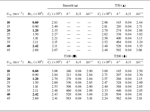


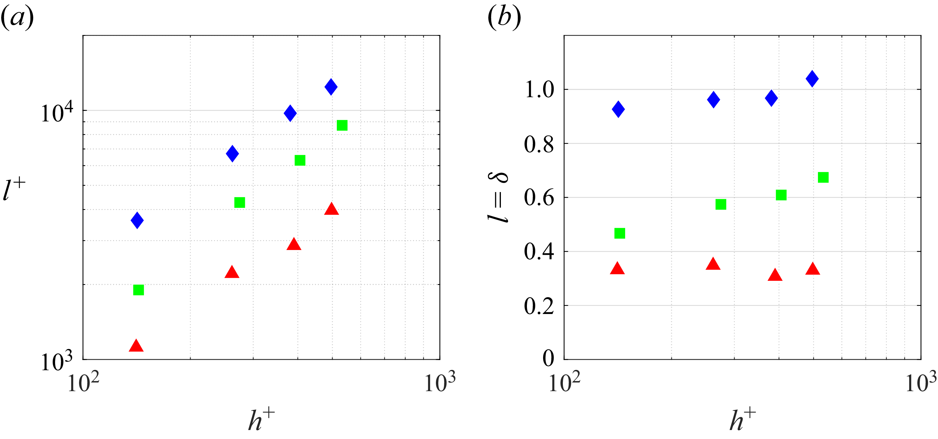


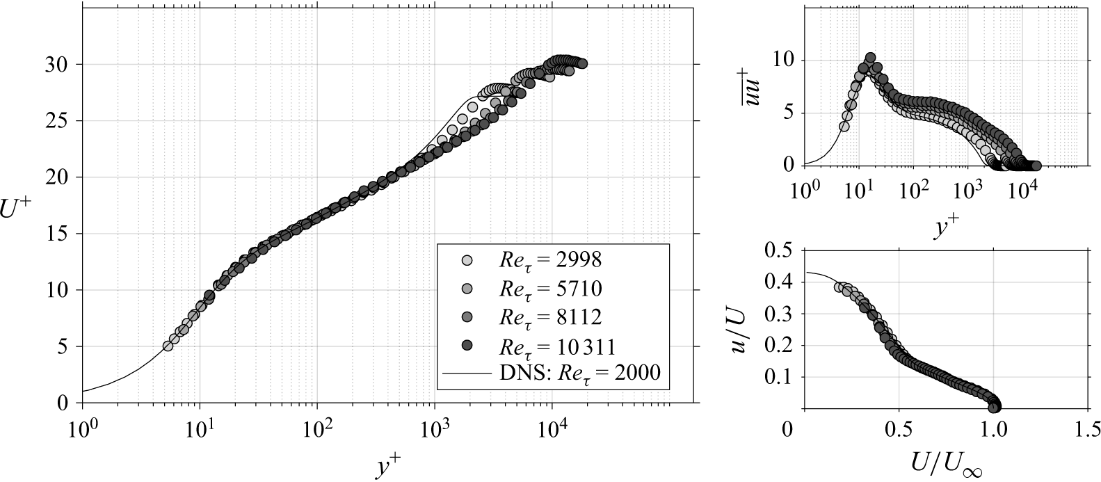

 Open access