

1 Introduction
1.1 Multiplicative Jensen’s formula
Let
 $f(z)$
be an analytic function given by
$f(z)$
be an analytic function given by
 $f(z)=\sum _k\hat {f}(k)z^k$
in
$f(z)=\sum _k\hat {f}(k)z^k$
in
 $D:=\{z:|z|<r\}$
. Suppose that
$D:=\{z:|z|<r\}$
. Suppose that
 $z_1$
,
$z_1$
,
 $z_2$
,
$z_2$
,
 $\cdots $
,
$\cdots $
,
 $z_n$
are the zeros of f in the interior of D repeated according to multiplicity.
$z_n$
are the zeros of f in the interior of D repeated according to multiplicity.
The classical Jensen’s formula, says that for any
 $0 \leq {\varepsilon }< \ln r$
,
$0 \leq {\varepsilon }< \ln r$
,
 $$ \begin{align} I_{\varepsilon}(f):=\frac{1}{2\pi}\int_0^{2\pi}\ln |f(e^{{\varepsilon}}e^{ix})|dx =I_0(f)-\sum_{\{i:0\leq \ln |z_i|<{{\varepsilon}}\}} \ln |z_i|+\#\{i:0\leq \ln |z_i|<{\varepsilon}\}{\varepsilon}.\end{align} $$
UsingFootnote
1
the ergodic theorem, the logarithmic integral on the left-hand side can be interpreted dynamically, as the limit of time averages along the trajectory of an ergodic dynamical system. In particular, given any irrational
 $\alpha $
, one can rewrite (1.1) as
$\alpha $
, one can rewrite (1.1) as
 $$ \begin{align} \nonumber & \lim\limits_{n\rightarrow\infty}\frac{1}{2\pi n} \int_0^{2\pi} \ln|f(e^{\varepsilon} e^{i(x+(n-1)\alpha)})\cdots f(e^{\varepsilon} e^{ix})|dx\\ =\ &I_0(f)- \sum_{\{i:0\leq \ln |z_i|<{{\varepsilon}}\}} \ln |z_i|+\#\{i:0\leq \ln |z_i|<{\varepsilon}\}{\varepsilon}. \end{align} $$
The left hand side of (1.2) can now be further interpreted as the complexified Lyapunov exponent of an analytic quasiperiodic
 $SL(1,{\mathbb {C}})$
cocycle
$SL(1,{\mathbb {C}})$
cocycle
 $(\alpha ,f):{\mathbb {T}}\,{\times}\, {\mathbb {C}}\to {\mathbb {T}}\,{\times}\, {\mathbb {C}}$
that acts via
$(\alpha ,f):{\mathbb {T}}\,{\times}\, {\mathbb {C}}\to {\mathbb {T}}\,{\times}\, {\mathbb {C}}$
that acts via
 $(\alpha ,f)(x,v)=(x+\alpha ,f(x)v).$
It is then natural to ask whether there is an analogous formula for the Lyapunov exponents of matrix-valued cocycles
 $(\alpha ,A)$
where A is an analytic matrix, the situation that is of course much more complicated since the commutativity is lost. The most intriguing question in this regard is what plays the role of zeros of analytic function f in the matrix-valued case.
$(\alpha ,A)$
where A is an analytic matrix, the situation that is of course much more complicated since the commutativity is lost. The most intriguing question in this regard is what plays the role of zeros of analytic function f in the matrix-valued case.
In this paper, we establish such formula for analytic Schrödinger cocycles. In reference to the relation between Birkhoff ergodic theorem and Kingman’s multiplicative ergodic theorem, we call it multiplicative Jensen’s formula.
Schrödinger cocycles play a central role in the analysis of one-dimensional discrete ergodic Schrödinger operators, a topic with origins in and a strong ongoing connection to physics and significant exciting recent advances, particularly in the analytic one-frequency quasiperiodic case.
Let
 $\alpha \in {\mathbb {R}}\backslash {\mathbb {Q}}$
,
$\alpha \in {\mathbb {R}}\backslash {\mathbb {Q}}$
,
 $x\in {\mathbb {R}},$
and V be a
$x\in {\mathbb {R}},$
and V be a
 $1$
-periodic real analytic function which can be analytically extended to the strip
$1$
-periodic real analytic function which can be analytically extended to the strip
 $\{z||\Im z|<h\}$
. A one-dimensional quasiperiodic Schrödinger operator
$\{z||\Im z|<h\}$
. A one-dimensional quasiperiodic Schrödinger operator
 $H_{V,x,\alpha }:\ell ^2({\mathbb {Z}})\to \ell ^2({\mathbb {Z}}) $
with one-frequency analytic potential is given by
$H_{V,x,\alpha }:\ell ^2({\mathbb {Z}})\to \ell ^2({\mathbb {Z}}) $
with one-frequency analytic potential is given by
 $$ \begin{align} (H_{V,x,\alpha}u)_n=u_{n+1}+u_{n-1}+V(x+n\alpha)u_n, \end{align} $$
The corresponding family of Schrödinger cocycles
 $(\alpha ,A_E):{\mathbb {T}}\times {\mathbb {C}}^2\to {\mathbb {T}}\times {\mathbb {C}}^2,\; E\in {\mathbb {R}}$
is defined by
$(\alpha ,A_E):{\mathbb {T}}\times {\mathbb {C}}^2\to {\mathbb {T}}\times {\mathbb {C}}^2,\; E\in {\mathbb {R}}$
is defined by
 $(\alpha ,A_E)(x,v)=(x+\alpha ,A_E(x)v)$
where
$(\alpha ,A_E)(x,v)=(x+\alpha ,A_E(x)v)$
where
 $$ \begin{align*} A_E(x)=\begin{pmatrix}E-V(x)&-1\\ 1&0\end{pmatrix}. \end{align*} $$
It governs the behavior of solutions to
 $$ \begin{align*} H_{V,x,\alpha}u=Eu.\end{align*} $$
The complexified Lyapunov exponent is given by
 $$ \begin{align} L_{\varepsilon}(E)=\lim\limits_{n\rightarrow\infty}\frac{1}{n} \int \ln \|A(x+i{\varepsilon}+(n-1)\alpha)\cdots A(x+i{\varepsilon})\|dx. \end{align} $$
The limit exists, as usual, by Kingman’s subadditive ergodic theorem. Complexified Lyapunov exponents were first studied by M. Herman [Reference Herman47], were crucial in the proofs of positivity of Lyapunov exponents at large couplings [Reference Sorets and Spencer77, Reference Bourgain and Goldstein23, Reference Bourgain21] and played a central role in Avila’s global theory [Reference Avila3].
We establish an analogue of (1.2) for
 $L_{\varepsilon }(E),$
where it turns out that the role of zeros of f in (1.1) is played by the (appropriate limits of) the Lyapunov exponents of the dual cocycles, an object that we prove to exist and call dual Lyapunov exponents.
$L_{\varepsilon }(E),$
where it turns out that the role of zeros of f in (1.1) is played by the (appropriate limits of) the Lyapunov exponents of the dual cocycles, an object that we prove to exist and call dual Lyapunov exponents.
The Aubry dual of the one-frequency Schrödinger operator (1.3) is
 $$ \begin{align} (\widehat{H}_{V,\theta,\alpha}u)_n=\sum\limits_{k=-\infty}^{\infty} V_k u_{n+k}+2\cos2\pi(\theta+n\alpha)u_n, \ \ n\in{\mathbb{Z}}. \end{align} $$
where
 $V_k$
is the k-th Fourier coefficient of
$V_k$
is the k-th Fourier coefficient of
 $V,$
see Sec 4.5 for details. For general analytic
$V,$
see Sec 4.5 for details. For general analytic
 $V,$
operator (1.5) is infinite-range, so its eigenequation
$V,$
operator (1.5) is infinite-range, so its eigenequation
 $\widehat {H}_{V,\theta ,\alpha }u=Eu$
does not define any finite-dimensional linear cocycle. However, if
$\widehat {H}_{V,\theta ,\alpha }u=Eu$
does not define any finite-dimensional linear cocycle. However, if
 $V(x)$
is a trigonometric polynomial of degree
$V(x)$
is a trigonometric polynomial of degree
 $d,$
the eigenequation
$d,$
the eigenequation
 $\widehat {H}_{V,\theta ,\alpha }u=Eu$
leads to a symplectic
$\widehat {H}_{V,\theta ,\alpha }u=Eu$
leads to a symplectic
 $2d$
-dimensional cocycle that we denote by
$2d$
-dimensional cocycle that we denote by
 $(\alpha ,\widehat {A}_E)$
. We denote its Lyapunov exponents by
$(\alpha ,\widehat {A}_E)$
. We denote its Lyapunov exponents by
 $\pm \hat {L}^d_{1}(E), \cdots , \pm \hat {L}^d_{d}(E)$
according to multiplicityFootnote
2
. We may assume
$\pm \hat {L}^d_{1}(E), \cdots , \pm \hat {L}^d_{d}(E)$
according to multiplicityFootnote
2
. We may assume
 $0\leq \hat {L}^d_1(E)\leq \cdots \leq \hat {L}^d_d(E)$
. We have
$0\leq \hat {L}^d_1(E)\leq \cdots \leq \hat {L}^d_d(E)$
. We have
Theorem 1.1. Assume
 $V(x)$
is a trigonometric polynomial of degree
$V(x)$
is a trigonometric polynomial of degree
 $d.$
For
$d.$
For
 $\alpha \in {\mathbb {R}}\backslash {\mathbb {Q}}$
and
$\alpha \in {\mathbb {R}}\backslash {\mathbb {Q}}$
and
 $(E,{\varepsilon })\in {\mathbb {R}}^2$
, we have
$(E,{\varepsilon })\in {\mathbb {R}}^2$
, we have
 $$ \begin{align} L_{{\varepsilon}}(E)= L_0(E) -\sum_{\{i:\hat{L}^d_i(E)< 2\pi |{\varepsilon}|\}} \hat{L}^d_i(E)+2\pi(\#\{i:\hat{L}^d_i(E)<2\pi|{\varepsilon}|\})|{\varepsilon}|. \end{align} $$
In fact, the multiplicative Jensen’s formula in Theorem 1.1 is not merely an analogue of the classical Jensen’s formula but a proper generalization, because zeros of the analytic function f can also be interpreted as the Lyapunov exponents of the dual cocycle. Indeed, consider the diagonal operator acting on
 $\ell ^2({\mathbb {Z}})$
 $$ \begin{align} (M_{x} u)_n=V(x+n\alpha)u_n, \ \ n\in{\mathbb{Z}}, \end{align} $$
where V is a
 $1$
-periodic real trigonometric polynomial of degree
$1$
-periodic real trigonometric polynomial of degree
 $d.$
Its Aubry dual is given by the Töplitz operator
$d.$
Its Aubry dual is given by the Töplitz operator
 $$ \begin{align} (\widehat{M} u)(n)=\sum\limits_{k=-d}^dV_ku_{n+k}, \ \ n\in{\mathbb{Z}}. \end{align} $$
It turns out that if
 $\{z_1(E),\cdots , z_d(E)\}$
are zeros of
$\{z_1(E),\cdots , z_d(E)\}$
are zeros of
 $V(z)=E$
with
$V(z)=E$
with
 $1\leq |z_i(E)|,$
Footnote
3
then
$1\leq |z_i(E)|,$
Footnote
3
then
 $\pm \ln |z_i|$
are precisely the Lyapunov exponents of the cocycle
$\pm \ln |z_i|$
are precisely the Lyapunov exponents of the cocycle
 $(\alpha ,\widehat {M})$
Footnote
4
of the eigenequation
$(\alpha ,\widehat {M})$
Footnote
4
of the eigenequation
 $\widehat {M}u=Eu,$
while
$\widehat {M}u=Eu,$
while
 $I_{{\varepsilon }}(E):=\int _{0}^{1}\ln |E-V(x+i|{\varepsilon }|)|dx$
is the complexified Lyapunov exponent of the
$I_{{\varepsilon }}(E):=\int _{0}^{1}\ln |E-V(x+i|{\varepsilon }|)|dx$
is the complexified Lyapunov exponent of the
 $SL(1,{\mathbb {C}})$
cocycle
$SL(1,{\mathbb {C}})$
cocycle
 $(\alpha ,V):{\mathbb {T}}\times {\mathbb {C}}\to {\mathbb {T}}\times {\mathbb {C}}$
acting via
$(\alpha ,V):{\mathbb {T}}\times {\mathbb {C}}\to {\mathbb {T}}\times {\mathbb {C}}$
acting via
 $(\alpha ,V)(x,v)=(x+\alpha ,V(x)v)$
.
$(\alpha ,V)(x,v)=(x+\alpha ,V(x)v)$
.
If V has infinitely many harmonics, we will use trigonometric polynomial approximation. Let
 $V^d(x)= \sum _{k=-d}^d \hat {V}_ke^{2\pi i kx}$
and let
$V^d(x)= \sum _{k=-d}^d \hat {V}_ke^{2\pi i kx}$
and let
 $\hat {L}^d_i(E)$
be the Lyapunov exponents of the corresponding dual
$\hat {L}^d_i(E)$
be the Lyapunov exponents of the corresponding dual
 $\mathrm {Sp_{2d}({\mathbb {C}})}$
cocycle. We have
$\mathrm {Sp_{2d}({\mathbb {C}})}$
cocycle. We have
Theorem 1.2 [The multiplicative Jensen’s formula].
For
 $\alpha \in {\mathbb {R}}\backslash {\mathbb {Q}}$
and
$\alpha \in {\mathbb {R}}\backslash {\mathbb {Q}}$
and
 $V\in C^\omega _h({\mathbb {T}},{\mathbb {R}})$
, there exist non-negative
$V\in C^\omega _h({\mathbb {T}},{\mathbb {R}})$
, there exist non-negative
 $\{\hat {L}_i(E)\}_{i=1}^m$
such that for any
$\{\hat {L}_i(E)\}_{i=1}^m$
such that for any
 $E\in {\mathbb {R}}$
 $$ \begin{align*}\hat{L}_i(E)=\lim\limits_{d\rightarrow \infty}\hat{L}^d_i(E), \ \ 1\leq i\leq m. \end{align*} $$
Moreover,
 $$ \begin{align*} L_{{\varepsilon}}(E)= L_0(E) -\sum_{\{i:\hat{L}_i(E)< 2\pi|{\varepsilon}|\}} \hat{L}_i(E)+2\pi(\#\{i:\hat{L}_i(E)<2\pi|{\varepsilon}|\})|{\varepsilon}| \end{align*} $$
for
 $|{\varepsilon }|<h$
.
$|{\varepsilon }|<h$
.
Remark 1.1. Note that the cocycle itself changes dramatically when d changes, with no limit in any of its components. However the Lyapunov exponents do converge to their limits, that we call dual Lyapunov exponents of (1.3).
Remark 1.2. One of the fundamental results in [Reference Avila3] is that
 $L_{\varepsilon }(E)$
is a piecewise affine function in
$L_{\varepsilon }(E)$
is a piecewise affine function in
 ${\varepsilon }$
for each E, and the slope of each piece is an integer. Theorem 1.2 quantifies this result, identifying the turning points with distinct
${\varepsilon }$
for each E, and the slope of each piece is an integer. Theorem 1.2 quantifies this result, identifying the turning points with distinct
 $\hat {L}_i$
’s, and the increments in the integer slopes with multiplicities of distinct
$\hat {L}_i$
’s, and the increments in the integer slopes with multiplicities of distinct
 $\hat {L}_i$
’s.
$\hat {L}_i$
’s.
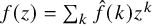
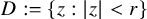
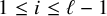
Indeed, for a fixed
 $E\in {\mathbb {R}}$
, assume that
$E\in {\mathbb {R}}$
, assume that
 $$ \begin{align*}0\leq \hat{L}_{k_1}<\hat{L}_{k_2}<\cdots<\hat{L}_{k_{\ell}} \end{align*} $$
and the multiplicity of each
 $\hat {L}_{k_i}$
is
$\hat {L}_{k_i}$
is
 $\{k_{i}-k_{i-1}\}_{i=1}^\ell $
with
$\{k_{i}-k_{i-1}\}_{i=1}^\ell $
with
 $k_0=0$
and
$k_0=0$
and
 $k_\ell =m$
. One may rewrite
$k_\ell =m$
. One may rewrite
 $L_{{\varepsilon }}(E)$
in Theorem 1.2 as the following piecewise affine function,
$L_{{\varepsilon }}(E)$
in Theorem 1.2 as the following piecewise affine function,
 $$ \begin{align}\small L_{{\varepsilon}}(E)=\left\{ \begin{aligned} & L_0(E) &|{\varepsilon}|\in \left[0,\frac{\hat{L}_{k_1}}{2\pi}\right],\\ &L_{\frac{\hat{L}_{k_i}}{2\pi}}(E)+2\pi k_{i}\left(|{\varepsilon}|-\frac{\hat{L}_{k_i}(E)}{2\pi}\right) &|{\varepsilon}|\in \left(\frac{\hat{L}_{k_{i}}}{2\pi},\frac{\hat{L}_{k_{i+1}}}{2\pi}\right],\\ &L_{\frac{\hat{L}_{k_\ell}}{2\pi}}(E)+2\pi k_\ell\left(|{\varepsilon}|-\frac{\hat{L}_{k_\ell}(E)}{2\pi}\right) &|{\varepsilon}|\in \left(\frac{\hat{L}_{k_\ell}}{2\pi},h\right). \end{aligned}\right. \end{align} $$
where
 $1\leq i\leq \ell -1$
. See pictures I-III for three different cases.
$1\leq i\leq \ell -1$
. See pictures I-III for three different cases.

1.2 Quantitative version of Avila’s global theory
The multiplicative Jensen’s formula not only sheds light on the global theory of one-frequency Schrödinger cocycles, but allows crucial advances in the study of the spectral theory of one-frequency Schrödinger operators (1.3).
In the past 40 years after the groundbreaking paper [Reference Dinaburg and Sinai29] the theory of quasiperiodic Schrödinger operators has been developed extensively, see [Reference Bourgain22, Reference Damanik27, Reference Jitomirskaya54, Reference Marx and Jitomirskaya69, Reference You79] for surveys of more recent results. For the one-frequency case, starting with [Reference Jitomirskaya51] and then [Reference Jitomirskaya53, Reference Bourgain and Goldstein23] the main thread has been to establish results nonperturbatively, that is, either in the regime of almost reducibility [Reference Puig70, Reference Puig71, Reference Avila and Jitomirskaya10, Reference Avila, Fayad and Krikorian8, Reference Hou and You49, Reference Avila4, Reference Avila5, Reference You79] or in the regime of positive Lyapunov exponent [Reference Jitomirskaya53, Reference Bourgain and Goldstein23, Reference Bourgain22, Reference Bourgain and Jitomirskaya25, Reference Goldstein and Schlag40, Reference Goldstein and Schlag41, Reference Goldstein and Schlag42, Reference Avila and Jitomirskaya9, Reference Jitomirskaya and Liu58, Reference Jitomirskaya and Liu59]. In 2015, Avila [Reference Avila3] gave a qualitative spectral picture, covering both regimes, based on the analysis of the asymptotic behavior of
 $L_{\varepsilon }(E)$
. The central concept in Avila’s global theory [Reference Avila3] is the acceleration
$L_{\varepsilon }(E)$
. The central concept in Avila’s global theory [Reference Avila3] is the acceleration
 $$ \begin{align*}\omega(E)=\lim\limits_{{\varepsilon}\rightarrow 0^+}\frac{L_{\varepsilon}(E)-L_0(E)}{2\pi{\varepsilon}}. \end{align*} $$
The global theory divided the spectra of one-frequency Schrödinger operator into three regimes based on the Lyapunov exponent and acceleration:
-
1. The subcritical regime:
 $L(E)=0$
and
$\omega (E)=0$
.
$L(E)=0$
and
$\omega (E)=0$
. -
2. The critical regime:
$L(E)=0$
and
$\omega (E)>0$
. -
3. The supercritical regime:
$L(E)>0$
and
$\omega (E)>0$
.


Moreover, the subcritical regime is equivalent to the almost reducible regime [Reference Avila4, Reference Avila5]. The critical regime is rare in the sense that it is a set of zero Lebesgue measure [Reference Avila3, Reference Avila and Krikorian12, Reference Jitomirskaya and Krasovsky57]. We will use the (sub/super)critical terminology both when referring to the energies E and to the corresponding cocycles
 $(\alpha ,A_E).$
Note that the global theory terminology was motivated by the study of the almost Mathieu operator (AMO), the central model in one-frequency quasiperiodic Schrödinger operators,
 $$ \begin{align} (H_{\lambda,x,\alpha}u)_n=u_{n+1}+u_{n-1}+2\lambda\cos2\pi(x+n\alpha)u_n,\ \ n\in{\mathbb{Z}}, \end{align} $$
where explicit computation [Reference Bourgain and Jitomirskaya24, Reference Avila3] shows that for all E in the spectrum, we have
-
1.
$|\lambda |<1$
:
$L(E)=0$
and
$\omega (E)=0$
. -
2.
$|\lambda |=1$
:
$L(E)=0$
and
$\omega (E)=1$
. -
3.
$|\lambda |>1$
:
$L(E)=\ln |\lambda |$
and
$\omega (E)=1$
.


Roughly speaking, Avila’s global theory is based on the picture of
 $L_{\varepsilon }(E)$
for
$L_{\varepsilon }(E)$
for
 ${\varepsilon }$
small enough. Our multiplicative Jensen’s formula actually not only gives the full picture of
${\varepsilon }$
small enough. Our multiplicative Jensen’s formula actually not only gives the full picture of
 $L_{\varepsilon }(E)$
for any
$L_{\varepsilon }(E)$
for any
 $|{\varepsilon }|<h$
, but also gives quantitative characterizations of several quantities in [Reference Avila3], such as the acceleration and the subcritical radius defined below.
$|{\varepsilon }|<h$
, but also gives quantitative characterizations of several quantities in [Reference Avila3], such as the acceleration and the subcritical radius defined below.
In particular, we can recharacterize Avila’s (sub/super)critical regimes in terms of the Lyapunov exponents
 $L(E)$
Footnote
5
and the smallest non-negative “dual Lyapunov exponent", without using the concept of acceleration:
$L(E)$
Footnote
5
and the smallest non-negative “dual Lyapunov exponent", without using the concept of acceleration:
Theorem 1.3. Assume
 $\alpha \in {\mathbb {R}}\backslash {\mathbb {Q}}$
and
$\alpha \in {\mathbb {R}}\backslash {\mathbb {Q}}$
and
 $V\in C_h^\omega ({\mathbb {T}},{\mathbb {R}})$
, then
$V\in C_h^\omega ({\mathbb {T}},{\mathbb {R}})$
, then
 $E\in {\mathbb {R}}$
is
$E\in {\mathbb {R}}$
is
-
1. Outside the spectrum Footnote 6 if
$L(E)>0$
and
$\hat {L}_1(E)>0$
, -
2. Supercritical if
$L(E)>0$
and
$\hat {L}_1(E)=0$
, -
3. Critical if
$L(E)=0$
and
$\hat {L}_1(E)=0$
, -
4. Subcritical if
$L(E)=0$
and
$\hat {L}_1(E)>0$
.


Remark 1.3. Item (4) implies that the Schrödinger cocycle
 $(\alpha ,A_E)$
is subcritical if and only if its “dual Lyapunov exponents” are all positive, which serves as the basis for the first author’s new proof of the almost reducibility conjecture [Reference Ge30].
$(\alpha ,A_E)$
is subcritical if and only if its “dual Lyapunov exponents” are all positive, which serves as the basis for the first author’s new proof of the almost reducibility conjecture [Reference Ge30].
We also give a new quantitative characterization of Avila’s acceleration:
Corollary 1.1. For
 $\alpha \in {\mathbb {R}}\backslash {\mathbb {Q}}, V\in C_h^\omega ({\mathbb {T}},{\mathbb {R}})$
, and any
$\alpha \in {\mathbb {R}}\backslash {\mathbb {Q}}, V\in C_h^\omega ({\mathbb {T}},{\mathbb {R}})$
, and any
 $E\in {\mathbb {R}}$
we have
$E\in {\mathbb {R}}$
we have
 $$ \begin{align*}\omega(E)=\begin{cases} 0 &\hat{L}_1(E)>0\\ \#\left\{j| \hat{L}_j(E)=0\right\} &\hat{L}_1(E)=0 \end{cases}. \end{align*} $$
Remark 1.4. The acceleration plays a crucial role in the study of supercritical Schrödinger operators. Corollary 1.1 shows that it is equal to the number of dual Lyapunov exponents that are equal to zero, or, for trigonometric polynomial V, to the dimension of the center of the corresponding cocycle. Generally speaking, although the definition of acceleration is clear, it is not easy to see why the acceleration is an integer outside the uniformly hyperbolic regime where it is simply equal to the winding number of a certain function. It is also difficult to compute the acceleration for specific cocycles. Corollary 1.1 provides another point of view which is more convenient, at least in the perturbative case (see Section 2.3 for further discussion).
In the study of subcritical Schrödinger operators, an important quantity is the so-called subcritical radius defined by
 $$ \begin{align*}h(E)=\sup\{|{\varepsilon}|:L_{\varepsilon}(E)=0\}. \end{align*} $$
It turns out it is also linked to dual Lyapunov exponents.
Corollary 1.2. For all
 $\alpha \in {\mathbb {R}}\backslash {\mathbb {Q}}$
,
$\alpha \in {\mathbb {R}}\backslash {\mathbb {Q}}$
,
 $V\in C_h^\omega ({\mathbb {T}},{\mathbb {R}}),$
and
$V\in C_h^\omega ({\mathbb {T}},{\mathbb {R}}),$
and
 $E\in {\mathbb {R}}$
, we have
$E\in {\mathbb {R}}$
, we have
 $h(E)=\frac {\hat {L}_1(E)}{2\pi }$
.
$h(E)=\frac {\hat {L}_1(E)}{2\pi }$
.
Remark 1.5. For subcritical almost Mathieu operator, it is explicitly computed in [Reference Avila3] that
 $$ \begin{align*}h(E)=\frac{\hat{L}_1(E)}{2\pi}=-\frac{\ln|\lambda|}{2\pi} \end{align*} $$
for all E in the spectrum, which plays an important role in several optimal estimates [Reference Ge, You and Zhou38, Reference Ge, You and Zhou39]. Corollary 1.2 is a generalization of this fact to general one-frequency Schrödinger operators.
1.3 Aubry duality
Our work can be viewed in a nutshell as the duality approach to Avila’s global theory. Aubry duality: a Fourier-type transform that links the direct integral in x of operators (1.3) to the direct integral in
 $\theta $
of operators (1.5) has had a long history since its original discovery by Aubry-Andre [Reference Aubry and Andre2] and has been explored and applied at many levels. Representing a certain gauge invariance of the underlying two-dimensional discrete operator in a perpendicular magnetic field [Reference Mandelshtam and Zhitomirskaya67], it has been understood at the level of integrated density of states, Lyapunov exponents, individual eigenfunctions and dynamics of individual cocycles, and explored in various qualitative and quantitative ways.
$\theta $
of operators (1.5) has had a long history since its original discovery by Aubry-Andre [Reference Aubry and Andre2] and has been explored and applied at many levels. Representing a certain gauge invariance of the underlying two-dimensional discrete operator in a perpendicular magnetic field [Reference Mandelshtam and Zhitomirskaya67], it has been understood at the level of integrated density of states, Lyapunov exponents, individual eigenfunctions and dynamics of individual cocycles, and explored in various qualitative and quantitative ways.
The almost Mathieu family stands out among other quasiperiodic operators (1.3) precisely because it is self-dual with respect to the Aubry duality, with
 $\hat {H}_{\lambda ,x,\alpha }=\lambda H_{\frac {1}{\lambda },x,\alpha },$
for example, [Reference Avron and Simon16]. In particular, the subcritical regime (
$\hat {H}_{\lambda ,x,\alpha }=\lambda H_{\frac {1}{\lambda },x,\alpha },$
for example, [Reference Avron and Simon16]. In particular, the subcritical regime (
 $|\lambda |<1$
) and the supercritical regime (
$|\lambda |<1$
) and the supercritical regime (
 $|\lambda |>1$
) are dual to each other, and this has been fruitfully explored in both directions. Aubry duality enables one to use the supercritical techniques (localization method) to deal with the subcritical problems [Reference Jitomirskaya53, Reference Puig70, Reference Puig71, Reference Avila and Jitomirskaya9, Reference Avila and Jitomirskaya10, Reference Ge and Kachkovskiy34], as well as the subcritical methods (almost reducibility) to study the supercritical problems [Reference Avila, You and Zhou14, Reference Avila, You and Zhou15, Reference Ge, You and Zhou38, Reference Ge, You and Zhao37, Reference Ge and You35, Reference Ge, You and Zhou39, Reference You79]. Even though the self-duality is destroyed when going beyond the almost Mathieu operator, many of the sub(super)critical results for the almost Mathieu operator can be generalized to (1.3) or (1.5). Based on the localization method for operator (1.5), one can get (almost) reducibility results for operators (1.3), see [Reference Bourgain and Jitomirskaya25, Reference Puig70, Reference Avila and Jitomirskaya10]. Almost reducibility for operator (1.3) in turn implies localization results for operator (1.5), see [Reference Avila, You and Zhou14, Reference Jitomirskaya and Kachkovskiy55, Reference Ge, You and Zhou38, Reference Ge, You and Zhou39, Reference Ge and You35]. Aubry duality therefore serves as a powerful bridge between (1.3) and (1.5).
$|\lambda |>1$
) are dual to each other, and this has been fruitfully explored in both directions. Aubry duality enables one to use the supercritical techniques (localization method) to deal with the subcritical problems [Reference Jitomirskaya53, Reference Puig70, Reference Puig71, Reference Avila and Jitomirskaya9, Reference Avila and Jitomirskaya10, Reference Ge and Kachkovskiy34], as well as the subcritical methods (almost reducibility) to study the supercritical problems [Reference Avila, You and Zhou14, Reference Avila, You and Zhou15, Reference Ge, You and Zhou38, Reference Ge, You and Zhao37, Reference Ge and You35, Reference Ge, You and Zhou39, Reference You79]. Even though the self-duality is destroyed when going beyond the almost Mathieu operator, many of the sub(super)critical results for the almost Mathieu operator can be generalized to (1.3) or (1.5). Based on the localization method for operator (1.5), one can get (almost) reducibility results for operators (1.3), see [Reference Bourgain and Jitomirskaya25, Reference Puig70, Reference Avila and Jitomirskaya10]. Almost reducibility for operator (1.3) in turn implies localization results for operator (1.5), see [Reference Avila, You and Zhou14, Reference Jitomirskaya and Kachkovskiy55, Reference Ge, You and Zhou38, Reference Ge, You and Zhou39, Reference Ge and You35]. Aubry duality therefore serves as a powerful bridge between (1.3) and (1.5).
All these methods and connections so far stayed firmly on the real territory, where both the operator and its dual are self-adjoint, so one can enjoy all the benefits of the spectral theory. Here we, for the first time, find the way to complexify the Aubry duality, or, alternatively, extend it to the non-self-adjoint setting, leading both to a new manifestation of it and a new empirical understanding, as well as a much deeper understanding of the existing manifestations.
Historically, Aubry duality was first formulated at the level of the integrated density of states, and thus, using the Thouless formula, the Lyapunov exponents. Namely, it was shown in [Reference Aubry and Andre2] (with the argument made rigorous in [Reference Avron and Simon16]) that for the almost Mathieu operator
 $H_{\lambda ,x,\alpha }$
given by (1.10), the following relation holds
$H_{\lambda ,x,\alpha }$
given by (1.10), the following relation holds
 $$ \begin{align} L(E) = {\hat{L}}(E)+\log|\lambda| \end{align} $$
A similar argument based on the Thouless formula for the strip [Reference Kotani and Simon63] leads to the beautiful Haro-Puig formula [Reference Haro and Puig46] for operators (1.3) with trigonometric polynomial
 $V(x)$
 $$ \begin{align} L(E)=\sum_{\{i:\hat{L}^d_i(E)>0\}} \hat{L}^d_i(E) +\ln |V_{d}|.\end{align} $$
Our multiplicative Jensen’s formula (1.9) can be manipulated into the Haro-Puig formula (1.12) for complexified Lyapunov exponents, but the latter cannot be seen in the framework of the previously existing proof, in absence of self-adjointness and the related spectral theory based invariance of the integrated density of states, so (1.12) in itself presents no compelling reason for (1.9) to hold.
We have found, however, that Aubry duality can be understood in a way that does not require any self-adjointness, leading to a new dynamical perspective on it and playing an important role in enabling various spectral applications.
We show that the fundamental way to see Aubry duality is through the invariance of the averaged Green’s function
 $$ \begin{align*}\int_{{\mathbb{T}}}\langle \delta_0,(H_{V(\cdot+i{\varepsilon}),x,\alpha}-E)^{-1}\delta_0\rangle dx = \int_{{\mathbb{T}}}\langle \delta_0, (\hat{H}_{V(\cdot+i{\varepsilon}),\theta,\alpha}-EI)^{-1}\delta_0\rangle d\theta, \end{align*} $$
something that can then be approached dynamically and combined with a non-self-adjoint version of the Johnson-Moser’s theorem [Reference Johnson and Moser62] that links averaged Green’s function to the derivative of the Lyapunov exponent, a strategy that we discuss more in Section 3.
The classical empirical understanding of Aubry duality is that Fourier transform takes nice normalizable eigenfunctions into Bloch waves and vice versa. Alternatively, (almost) localized eigenfunctions correspond to (almost) reducibility for the dual cocycle, and vice versa, something that by now has almost became a folklore. Here we present a similarly compelling heuristic – a new perspective – that was behind our discovery of the multiplicative Jensen’s formula.
Assume that
 $(\alpha , \widehat {A}_{E})$
is analytically conjugated to the form:
$(\alpha , \widehat {A}_{E})$
is analytically conjugated to the form:
 $$ \begin{align} Z(\theta+\alpha)^{-1} \widehat{A}_{E}(\theta)Z(\theta) = \left( \begin{array}{ccccccc} e^{\gamma} & 0& \quad \\ 0 & e^{-\gamma} & \quad \\ \quad & \quad & D(\theta) \end{array} \right) .\end{align} $$
By Aubry duality, it implies that
 $$ \begin{align*} (H_{V,x+i\gamma,\alpha}u)_n=u_{n+1}+u_{n-1}+V(x+i\gamma+n\alpha)u_n, \end{align*} $$
has a localized eigenfunction. Therefore the Schrödinger cocycle
 $(\alpha , A_E(x+i\gamma )) $
is nonuniformly hyperbolic, so
$(\alpha , A_E(x+i\gamma )) $
is nonuniformly hyperbolic, so
 $L_{{\varepsilon }}(E)$
cannot be affine at
$L_{{\varepsilon }}(E)$
cannot be affine at
 ${\varepsilon }=\gamma ,$
therefore
${\varepsilon }=\gamma ,$
therefore
 $\gamma $
must be the turning point of
$\gamma $
must be the turning point of
 $L_{{\varepsilon }}(E)$
. But of course (1.13) just means
$L_{{\varepsilon }}(E)$
. But of course (1.13) just means
 $\gamma $
is the Lyapunov exponent of the dual cocycle
$\gamma $
is the Lyapunov exponent of the dual cocycle
 $(\alpha , \widehat {A}_{E})$
. While not fully rigorous, we see this argument as inspirational to our approach, and in fact it plays an important role both in the final proof and a physics application [Reference Liu, Wang, Liu, Zhou and Chen64, Reference Liu, Zhou and Chen65].
$(\alpha , \widehat {A}_{E})$
. While not fully rigorous, we see this argument as inspirational to our approach, and in fact it plays an important role both in the final proof and a physics application [Reference Liu, Wang, Liu, Zhou and Chen64, Reference Liu, Zhou and Chen65].
1.4 Bochi-Viana Theorem for dual cocycles and partial hyperbolicity
Both our proof of Theorem 1.1 and an important starting point for the most interesting corollaries is based on the study of the dynamics of dual cocycles, which turns out to have a remarkable universal property.
It is a general program, first outlined by Mañé [Reference Mañé68] and developed by Bochi-Viana [Reference Bochi and Viana19] that, when applied to linear cocycles, states that for
 $C^0$
generic
$C^0$
generic
 $\mathrm {GL_d({\mathbb {C}})}$
cocycles over any measure preserving transformation the Oseledets splitting (see section 4.2 for the definitions in this setting) is either trivial or dominated. While this result definitely hinges on low regularity considerations (and counterexamples in higher regularity do exist), it was shown in [Reference Avila, Jitomirskaya and Sadel11] that Bochi-Viana theorem also holds – and in a much stronger form – for analytic one-frequency cocycles: the Oseledec splitting is either trivial or dominated on an open and dense set of such cocycles.
$\mathrm {GL_d({\mathbb {C}})}$
cocycles over any measure preserving transformation the Oseledets splitting (see section 4.2 for the definitions in this setting) is either trivial or dominated. While this result definitely hinges on low regularity considerations (and counterexamples in higher regularity do exist), it was shown in [Reference Avila, Jitomirskaya and Sadel11] that Bochi-Viana theorem also holds – and in a much stronger form – for analytic one-frequency cocycles: the Oseledec splitting is either trivial or dominated on an open and dense set of such cocycles.
Here we show that something stronger yet holds for the dual cocycles. Let
 ${\mathbb {C}}_+$
denote
${\mathbb {C}}_+$
denote
 $\{E\in {\mathbb {C}}|\Im E>0\}.$
For
$\{E\in {\mathbb {C}}|\Im E>0\}.$
For
 $V(x)$
a trigonometric polynomial of degree
$V(x)$
a trigonometric polynomial of degree
 $d,$
let
$d,$
let
 $$ \begin{align*}0\leq \hat{L}_{k_1}<\hat{L}_{k_2}<\cdots<\hat{L}_{k_{\ell}} \end{align*} $$
be the listing of all nonnegative dual Lyapunov exponents, where the multiplicity of each
 $\hat {L}_{k_i}$
is
$\hat {L}_{k_i}$
is
 $\{k_{i}-k_{i-1}\}_{i=1}^\ell $
with
$\{k_{i}-k_{i-1}\}_{i=1}^\ell $
with
 $k_0=0$
and
$k_0=0$
and
 $k_\ell =d$
.
$k_\ell =d$
.
Theorem 1.4. Let
 $V(x)$
be a trigonometric polynomial of degree
$V(x)$
be a trigonometric polynomial of degree
 $d.$
Then the dual cocycle
$d.$
Then the dual cocycle
 $(\alpha ,\widehat {A}_{E})$
is always
$(\alpha ,\widehat {A}_{E})$
is always
-
1.
$(d-k_i)$
-dominated for all
$ 0\leq i \leq \ell ,$
for
$E\in {\mathbb {C}}_+$
; -
2. either trivial or
$(d-k_i)$
-dominated for all
$1\leq i \leq \ell ,$
for
$E\in {\mathbb {R}}.$


Remark 1.6. For
 $E\in {\mathbb {C}}_+$
the cocycle is obviously uniformly hyperbolic, so d-dominated, but the domination at all other levels is a nontrivial statement.
$E\in {\mathbb {C}}_+$
the cocycle is obviously uniformly hyperbolic, so d-dominated, but the domination at all other levels is a nontrivial statement.
In particular, we have
Corollary 1.3. The acceleration
 $\omega (E)>0$
if and only if the dual
$\omega (E)>0$
if and only if the dual
 $\mathrm {Sp_{2d}({\mathbb {C}})}$
cocycle
$\mathrm {Sp_{2d}({\mathbb {C}})}$
cocycle
 $(\alpha ,\widehat {A}_{E})$
is partially hyperbolic with zero center Lyapunov exponents.
$(\alpha ,\widehat {A}_{E})$
is partially hyperbolic with zero center Lyapunov exponents.
1.5 A spectral application
In this subsection, we give a sample direct spectral application of our quantitative global theory: a new elegant characterization of the spectrum of
 $H_{V,x,\alpha }$
and a criterion for uniformity of corresponding Schrödinger cocycles.
$H_{V,x,\alpha }$
and a criterion for uniformity of corresponding Schrödinger cocycles.
It is well-known that the spectrum of
 $H_{V,x,\alpha },$
denoted as
$H_{V,x,\alpha },$
denoted as
 $\Sigma _{V,\alpha },$
is an x-independent set [Reference Avron and Simon16]. The classical Johnson’s theorem [Reference Jonhnson61] characterizes the spectrum as
$\Sigma _{V,\alpha },$
is an x-independent set [Reference Avron and Simon16]. The classical Johnson’s theorem [Reference Jonhnson61] characterizes the spectrum as
 $$ \begin{align*}\Sigma_{V,\alpha}=\{E\in{\mathbb{R}}: L(E)=0\ \ \mbox{or}\ \ (\alpha, A_E)\ \ \mbox{is non uniformly hyperbolic}\}. \end{align*} $$
Nonuniform hyperbolicity is generally difficult to capture. It turns out however that it is determined precisely by the lowest dual Lyapunov exponent. We have
Corollary 1.4. For any
 $\alpha \in {\mathbb {R}}\backslash {\mathbb {Q}}$
and
$\alpha \in {\mathbb {R}}\backslash {\mathbb {Q}}$
and
 $V\in C_h^\omega ({\mathbb {T}},{\mathbb {R}})$
, then
$V\in C_h^\omega ({\mathbb {T}},{\mathbb {R}})$
, then
 $$ \begin{align*}\Sigma_{V,\alpha}=\{E\in{\mathbb{R}}: L(E)\cdot \hat{L}_1(E)=0\}. \end{align*} $$
An equivalent formulation of Corollary 1.4 is the following criterion for uniformity of Schrödinger cocycles. We recall that an
 $SL(2,{\mathbb {C}})$
cocycle
$SL(2,{\mathbb {C}})$
cocycle
 $(\alpha ,A)$
is uniform if the convergence
$(\alpha ,A)$
is uniform if the convergence
 $$ \begin{align*}\lim\limits_{n\rightarrow \infty }\frac{1}{n}\ln\|A(x+(n-1)\alpha)\cdots A(x)\|=L(\alpha,A) \end{align*} $$
holds for all
 $x\in {\mathbb {T}}$
and is uniform (see, e.g., [Reference Damanik and Lenz28] for a discussion). Since Schrödinger cocycles
$x\in {\mathbb {T}}$
and is uniform (see, e.g., [Reference Damanik and Lenz28] for a discussion). Since Schrödinger cocycles
 $(\alpha ,A_E)$
are uniform for E outside the spectrum or in the set where
$(\alpha ,A_E)$
are uniform for E outside the spectrum or in the set where
 $L(E)=0$
(e.g., [Reference Damanik and Lenz28, Corollary A.3]), an immediate consequence of Corollary 1.4 is
$L(E)=0$
(e.g., [Reference Damanik and Lenz28, Corollary A.3]), an immediate consequence of Corollary 1.4 is
Corollary 1.5. A Schrödinger cocycle
 $(\alpha ,A_E)$
with
$(\alpha ,A_E)$
with
 $\hat {L}_1(E)>0$
is always uniform.
$\hat {L}_1(E)>0$
is always uniform.
Remark 1.7. If V is a trigonometric polynomial, this can be nicely reformulated as “ A Schrödinger cocycle with hyperbolic dual cocycle is always uniform.”
Most excitingly, however, our analysis enables us to extend some of the most famous almost Mathieu results to large classes of quasiperiodic operators.
In particular, in the companion paper [Reference Ge, Jitomirskaya and You33] we develop machinery to prove the Ten Martini problem (i.e., Cantor spectrum without any parameter exclusion) for a large explicitly defined open set of both sub- and supercritical quasiperiodic operators, so called operators of type 1. The Ten Martini problem has so far only been established for the almost Mathieu operator through a combination of Liouville and Diophantine approaches that were both almost Mathieu specific and only quite miraculously met in the middle. It has not even been universally expected that it holds for all parameters for anything other than the almost Mathieu operator.
In [Reference Ge and Jitomirskaya32] we prove sharp arithmetic spectral transition, as in [Reference Avila, You and Zhou14, Reference Jitomirskaya and Liu58, Reference Jitomirskaya and Liu59] for all operators of type 1, without further assumptions.
Finally, these results enable a new and simple proof of Avila’s almost reducibility conjecture for Schrödinger cocycles [Reference Ge30]. With subcriticality guaranteeing
 $\hat {L}_1>0,$
the proof proceeds through establishing nonperturbative almost localization for the dual operator and is optimal for the case of trigonometric polynomial V (i.e., does not require shrinking of the band).
$\hat {L}_1>0,$
the proof proceeds through establishing nonperturbative almost localization for the dual operator and is optimal for the case of trigonometric polynomial V (i.e., does not require shrinking of the band).
The results and some applications were presented at multiple venues, including the Anosov-85 meeting (November 2021), the BIRS workshop on Almost-Periodic Spectral Problems (April 2022), ICM 2022, and QMath 15 (2022), and announced in [Reference Jitomirskaya54] in January 2022. A different proof of formula (1.9) for trigonometric polynomials appeared in [Reference Han and Schlag45]. Several applications of our results, including those in [Reference Liu, Wang, Liu, Zhou and Chen64, Reference Liu, Zhou and Chen65, Reference Wang, Wang, You and Zhou78], have since been developed, and further applications are ongoing.
The rest of this paper is organized as follows. Section 2 contains further spectral and physics applications. In Section 3, we introduce the main ideas of the proof. Section 4 contains the preliminaries. In Section 5, we study the Green’s function of general finite-range Schrödinger operators, while in Section 6 we study the Green’s function for non-self-adjoint quasiperiodic operators. In Section 7, we prove the main results, postponing proofs of the remaining results to Section 8. Finally, we prove Johnson-Moser’s theorem for Schrödinger operators on the strip (Proposition 5.3) in Section 9, and prove the representation of the Green’s function for general strip operators (Lemma 6.2) in Section 10.
2 Other applications
2.1 Arithmetic Anderson localization
Our results allow us to make spectral conclusions both for
 $H_{V,x,\alpha }$
and
$H_{V,x,\alpha }$
and
 $\widehat {H}_{V,\theta ,\alpha }$
. Here we present a sample result on Anderson localization for
$\widehat {H}_{V,\theta ,\alpha }$
. Here we present a sample result on Anderson localization for
 $\widehat {H}_{V,\theta ,\alpha }$
, which was extensively studied [Reference Avila and Jitomirskaya10, Reference Ge, You and Zhou38, Reference Bourgain and Jitomirskaya24, Reference Chulaevsky and Dinaburg26, Reference Jitomirskaya and Kachkovskiy55, Reference Bourgain22, Reference Ge and You35] since the 1980s. All the existing results are “local” in the sense that one needs to assume there is a large coupling constant
$\widehat {H}_{V,\theta ,\alpha }$
, which was extensively studied [Reference Avila and Jitomirskaya10, Reference Ge, You and Zhou38, Reference Bourgain and Jitomirskaya24, Reference Chulaevsky and Dinaburg26, Reference Jitomirskaya and Kachkovskiy55, Reference Bourgain22, Reference Ge and You35] since the 1980s. All the existing results are “local” in the sense that one needs to assume there is a large coupling constant
 $\lambda $
before the
$\lambda $
before the
 $\cos $
potential. Moreover most of the results cannot go beyond the Diophantine frequencies. We give a global result, starting from the positivity of the Lyapunov exponents. Let
$\cos $
potential. Moreover most of the results cannot go beyond the Diophantine frequencies. We give a global result, starting from the positivity of the Lyapunov exponents. Let
 $$ \begin{align*}\beta=\beta(\alpha)=\limsup\limits_{k\rightarrow \infty}-\frac{\ln\|k\alpha\|_{{\mathbb{R}}/{\mathbb{Z}}}}{|k|}. \end{align*} $$
For a given irrational number
 $\alpha $
, we say
$\alpha $
, we say
 $\theta \in (0,1)$
is
$\theta \in (0,1)$
is
 $\alpha $
-Diophantine if there exist
$\alpha $
-Diophantine if there exist
 $\kappa>0$
and
$\kappa>0$
and
 $\tau>1$
such that
$\tau>1$
such that
 $$ \begin{align*}\|2\theta+k\alpha\|_{{\mathbb{R}}/{\mathbb{Z}}}>\frac{\kappa}{(|k|+1)^\tau}, \end{align*} $$
for any
 $k\in {\mathbb {Z}}$
, where
$k\in {\mathbb {Z}}$
, where
 $\|x\|_{{\mathbb {R}}/{\mathbb {Z}}}=\text {dist}(x,{\mathbb {Z}}).$
Clearly, for any fixed irrational number
$\|x\|_{{\mathbb {R}}/{\mathbb {Z}}}=\text {dist}(x,{\mathbb {Z}}).$
Clearly, for any fixed irrational number
 $\alpha $
, the set of phases which are
$\alpha $
, the set of phases which are
 $\alpha $
-Diophantine is of full Lebesgue measure.
$\alpha $
-Diophantine is of full Lebesgue measure.
Corollary 2.1. If
 $\hat {L}_1(E)>\beta >0$
for all
$\hat {L}_1(E)>\beta >0$
for all
 $E\in {\mathbb {R}}$
, then
$E\in {\mathbb {R}}$
, then
 $\widehat {H}_{V,\alpha ,\theta }$
has Anderson localization for
$\widehat {H}_{V,\alpha ,\theta }$
has Anderson localization for
 $\alpha $
-Diophantine
$\alpha $
-Diophantine
 $\theta $
.
$\theta $
.
Remark 2.1. For the almost Mathieu operator, Corollary 2.1 is what is now sometimes called the Andre-Aubry-Jitomirskaya conjecture [Reference Aubry and Andre2, Reference Jitomirskaya52] which was proved in [Reference Jitomirskaya and Liu58], see also [Reference Ge, You and Zhao37] for a new proof.
Remark 2.2. The limitation
 $\beta>0$
comes from our reliance in the proof on a theorem of [Reference Ge, You and Zhao37], who in turn rely on Avila’s proof of the almost reducibility conjecture for Liouville
$\beta>0$
comes from our reliance in the proof on a theorem of [Reference Ge, You and Zhao37], who in turn rely on Avila’s proof of the almost reducibility conjecture for Liouville
 $\alpha $
[Reference Avila4]. This limitation has been removed in the follow-up paper by the first author [Reference Ge30] through a direct localization-side proof for
$\alpha $
[Reference Avila4]. This limitation has been removed in the follow-up paper by the first author [Reference Ge30] through a direct localization-side proof for
 $\beta =0.$
Remark 2.3. We present the result for
 $\alpha $
-Diophantine
$\alpha $
-Diophantine
 $\theta $
rather than a slightly weaker optimal [Reference Jitomirskaya and Liu58] condition
$\theta $
rather than a slightly weaker optimal [Reference Jitomirskaya and Liu58] condition
 $\delta (\alpha ,\theta )=0$
where
$\delta (\alpha ,\theta )=0$
where
 $$ \begin{align*}\delta(\alpha,\theta)=\limsup_{k\to\infty} -\frac{\ln ||2\theta+ k\alpha||_{{\mathbb{R}}/{\mathbb{Z}}}}{|k|},\end{align*} $$
because the authors of [Reference Ge, You and Zhao37] choose a similar limitation. The theorem in fact holds under the
 $\delta (\alpha ,\theta )=0$
condition with a little more technical effort.
$\delta (\alpha ,\theta )=0$
condition with a little more technical effort.
2.2 An application to the Soukoulis-Economou’s model
We can also make immediate conclusions for the Soukoulis-Economou’s model (SEM)
 $$ \begin{align} (H_{\alpha,x}u)(n)=u(n+1)+u(n-1)+2\lambda_1\cos2\pi(x+n\alpha)u(n)+2\lambda_2\cos 4\pi(x+n\alpha)u(n). \end{align} $$
It is also known in physics literature as generalized Harper’s model (e.g., [Reference Hiramoto and Kohmoto48, Reference Soukoulis and Economou76]), which is of special interest because of its connection to the three-dimensional quantum Hall effect [Reference Hiramoto and Kohmoto48, Reference Soukoulis and Economou76]. The Lyapunov exponents for this model have been studied in [Reference Jitomirskaya and Liu60, Reference Marx, Shou and Wellens75].
The Aubry dual of (2.1) is
 $$ \begin{align} (\widehat{H}_{\theta,\alpha}u)(n)=\lambda_2u(n-2)+\lambda_1u(n-1)+\lambda_1u(n+1)+\lambda_2u(n+2)+2\cos2\pi(\theta+n\alpha)u_n, \ \ n\in{\mathbb{Z}}. \end{align} $$
The operator (2.2) is a 4-th order difference operator, and we denote the non-negative Lyapunov exponent of the associated cocycle by
 $\hat {L}_2(E)\geq \hat {L}_1(E)\geq 0$
.
$\hat {L}_2(E)\geq \hat {L}_1(E)\geq 0$
.
Corollary 2.2. For SEM operator with
 $\alpha \in {\mathbb {R}}\backslash {\mathbb {Q}},$
for any
$\alpha \in {\mathbb {R}}\backslash {\mathbb {Q}},$
for any
 $E\in {\mathbb {R}}$
,
$E\in {\mathbb {R}}$
,
 $\omega (E)=2$
if and only if
$\omega (E)=2$
if and only if
 $L(E)=\ln |\lambda _2|$
and
$L(E)=\ln |\lambda _2|$
and
 $|\lambda _2|\geq 1$
.
$|\lambda _2|\geq 1$
.
Corollary 2.3. For
 $\alpha \in {\mathbb {R}}\backslash {\mathbb {Q}}$
and
$\alpha \in {\mathbb {R}}\backslash {\mathbb {Q}}$
and
 $|\lambda _2|< 1,$
the energies in the spectrum of SEM are in one of the following three regimes:
$|\lambda _2|< 1,$
the energies in the spectrum of SEM are in one of the following three regimes:
-
1. Subcritical regime:
$L(E)=0$
and
$\omega (E)=0$
. -
2. Critical regime:
$L(E)=0$
and
$\omega (E)=1$
. -
3. Supercritical regime:
$L(E)>0$
and
$\omega (E)=1$
.


Remark 2.4. In this case, the crucial point is that the acceleration is always no more than
 $1,$
which is also a key feature of the almost Mathieu operator. In particular, this means that supercritical SEM with
$1,$
which is also a key feature of the almost Mathieu operator. In particular, this means that supercritical SEM with
 $|\lambda _2|<1$
is of type 1 in the sense of [Reference Ge, Jitomirskaya and You33], and it makes it possible to generalize many almost Mathieu results to this case. We note that the supercritical regime is known to hold under explicit conditions on
$|\lambda _2|<1$
is of type 1 in the sense of [Reference Ge, Jitomirskaya and You33], and it makes it possible to generalize many almost Mathieu results to this case. We note that the supercritical regime is known to hold under explicit conditions on
 $\lambda _1,\lambda _2$
with
$\lambda _1,\lambda _2$
with
 $|\lambda _2|< 1$
[Reference Jitomirskaya and Liu60] requiring, in particular,
$|\lambda _2|< 1$
[Reference Jitomirskaya and Liu60] requiring, in particular,
 $\lambda _1>100\lambda _2$
. Our analysis of type 1 operators applies to the entire regime
$\lambda _1>100\lambda _2$
. Our analysis of type 1 operators applies to the entire regime
 $|\lambda _2|< 1$
.
$|\lambda _2|< 1$
.
2.3 A further characterization of the acceleration
Let V be a trigonometric polynomial of degree d such that
 $\widehat {A}_{E}$
is almost reducible to some constant matrix
$\widehat {A}_{E}$
is almost reducible to some constant matrix
 $\tilde {A}$
in the sense that there exists
$\tilde {A}$
in the sense that there exists
 $B_n\in C^\omega _{r_n}({\mathbb {T}},\mathrm {GL_{2d}({\mathbb {C}}))}$
for some
$B_n\in C^\omega _{r_n}({\mathbb {T}},\mathrm {GL_{2d}({\mathbb {C}}))}$
for some
 $r_n>0$
such that
$r_n>0$
such that
 $$ \begin{align*}\|B_n(\theta+\alpha)^{-1}\widehat{A}_{E}(\theta)B_n(\theta)-\tilde{A}\|_{r_n}\rightarrow 0.\end{align*} $$
Note that this assumption is always satisfied for a positive measure set of
 $\alpha $
if
$\alpha $
if
 $V=\lambda f$
and
$V=\lambda f$
and
 $\lambda $
is sufficiently small. In this case, the dual Lyapunov exponents can be computed explicitly, and the multiplicative Jensen’s formula takes a particularly elegant form
$\lambda $
is sufficiently small. In this case, the dual Lyapunov exponents can be computed explicitly, and the multiplicative Jensen’s formula takes a particularly elegant form
Corollary 2.4. Suppose that
 $E\in {\mathbb {R}}$
,
$E\in {\mathbb {R}}$
,
 $\alpha \in {\mathbb {R}}\backslash {\mathbb {Q}}$
and
$\alpha \in {\mathbb {R}}\backslash {\mathbb {Q}}$
and
 $(\alpha ,\widehat {A}_{E})$
is almost reducible to some constant matrix
$(\alpha ,\widehat {A}_{E})$
is almost reducible to some constant matrix
 $\tilde {A}$
. Let
$\tilde {A}$
. Let
 $\lambda _1, \cdots , \lambda _d$
be the eigenvalues of
$\lambda _1, \cdots , \lambda _d$
be the eigenvalues of
 $\tilde {A}$
, counting the multiplicity, with
$\tilde {A}$
, counting the multiplicity, with
 $1\leq |\lambda _1|\leq \cdots \leq |\lambda _d|$
. Then
$1\leq |\lambda _1|\leq \cdots \leq |\lambda _d|$
. Then
 $$ \begin{align*} L_{{\varepsilon}}(E)= L_0(E) -\sum_{\{i:\ln |\lambda_i|< 2\pi |{\varepsilon}|\}} \ln|\lambda_i|+2\pi (\#\{i:\ln|\lambda_i|<2\pi|{\varepsilon}|\})|{\varepsilon}|. \end{align*} $$
Corollary 2.5. Under the assumptions of Corollary 2.4, we have
 $$ \begin{align*}\omega(E)=\begin{cases} 0 &|\lambda_1|>1\\ \#\left\{j| |\lambda_j|=1\right\} &|\lambda_1|=1 \end{cases}. \end{align*} $$
Remark 2.5. The acceleration is nothing but the number of pairs of eigenvalues of
 $\tilde A$
lying in the unit circle.
$\tilde A$
lying in the unit circle.
2.4 A physics application
Our results allow a number of interesting physics applications. Here we mention the application of Theorem 1.1 and Theorem 1.2 to non-Hermitian crystals. While Hermiticity lies at the heart of quantum mechanics, recent experimental advances in controlling dissipation have brought about unprecedented flexibility in engineering non-Hermitian Hamiltonians in open classical and quantum systems [Reference Gong, Ashida, Kawabata, Takasan, Higashikawa and Ueda43]. Non-Hermitian Hamiltonians exhibit rich phenomena without Hermitian analogues: for example, parity-time (
 $\mathcal {PT}$
) symmetry breaking, topological phase transition, non-Hermitian skin effects, etc. [Reference Ashidaa, Gong and Ueda1, Reference Bergholtz, Budich and Kunst18], and all of these phenomena can be observed in non-Hermitian crystals [Reference Longhi66, Reference Jiang, Lang, Yang, Zhu and Chen50].
$\mathcal {PT}$
) symmetry breaking, topological phase transition, non-Hermitian skin effects, etc. [Reference Ashidaa, Gong and Ueda1, Reference Bergholtz, Budich and Kunst18], and all of these phenomena can be observed in non-Hermitian crystals [Reference Longhi66, Reference Jiang, Lang, Yang, Zhu and Chen50].
Here, we consider the non-Hermitian crystals of the form
 $$ \begin{align} (H_{V,x+i{\varepsilon},\alpha}u)_n=u_{n+1}+u_{n-1}+V(x+i{\varepsilon}+n\alpha)u_n. \end{align} $$
This defines a nonself adjoint operator on
 $\ell ^2({\mathbb {Z}})$
. An important class of non-Hermitian Hamiltonians which have recently attracted a significant attention in physics is called parity-time (
$\ell ^2({\mathbb {Z}})$
. An important class of non-Hermitian Hamiltonians which have recently attracted a significant attention in physics is called parity-time (
 $\mathcal {PT}$
) symmetry Hamiltonian (i.e.,
$\mathcal {PT}$
) symmetry Hamiltonian (i.e.,
 $\overline {v}(n)=v(-n)$
, [Reference Bender and Boettcher17]). Indeed, if V is even with
$\overline {v}(n)=v(-n)$
, [Reference Bender and Boettcher17]). Indeed, if V is even with
 $x=0$
, (2.3) is a
$x=0$
, (2.3) is a
 $\mathcal {PT}$
symmetry Hamiltonian. Different from the self-adjoint operators, the spectra of non-self-adjoint operators may not always consist of real numbers, and physicists are interested in the phase transition from real energy spectrum (unbroken
$\mathcal {PT}$
symmetry Hamiltonian. Different from the self-adjoint operators, the spectra of non-self-adjoint operators may not always consist of real numbers, and physicists are interested in the phase transition from real energy spectrum (unbroken
 $\mathcal {PT}$
phase) to complex energy spectrum (broken
$\mathcal {PT}$
phase) to complex energy spectrum (broken
 $\mathcal {PT}$
phase), that is,
$\mathcal {PT}$
phase), that is,
 $\mathcal {PT}$
symmetry breaking phase transition [Reference Longhi66]. As first discovered in [Reference Liu, Wang, Liu, Zhou and Chen64], this kind of transition can be studied through the analysis of Lyapunov exponents
$\mathcal {PT}$
symmetry breaking phase transition [Reference Longhi66]. As first discovered in [Reference Liu, Wang, Liu, Zhou and Chen64], this kind of transition can be studied through the analysis of Lyapunov exponents
 $L_{{\varepsilon }}(E)$
. Theorem 1.2 allows to easily deduce that subcritical radius
$L_{{\varepsilon }}(E)$
. Theorem 1.2 allows to easily deduce that subcritical radius
 $$ \begin{align*}\min_{E \in\Sigma_{V,\alpha}} h(E)= \frac{1}{2\pi} \min_{E \in\Sigma_{V,\alpha}} \hat{L}_1(E)\end{align*} $$
is the
 $\mathcal {PT}$
symmetry breaking parameter (one may consult [Reference Liu, Wang, Liu, Zhou and Chen64, Reference Liu, Zhou and Chen65] for the detailed reasoning).
$\mathcal {PT}$
symmetry breaking parameter (one may consult [Reference Liu, Wang, Liu, Zhou and Chen64, Reference Liu, Zhou and Chen65] for the detailed reasoning).
Another way to understand parity-time (
 $\mathcal {PT}$
) symmetry breaking is topological phase transition. Let
$\mathcal {PT}$
) symmetry breaking is topological phase transition. Let
 $E_B\in {\mathbb {R}}$
be a base energy which is not in the spectrum of
$E_B\in {\mathbb {R}}$
be a base energy which is not in the spectrum of
 $H.$
We introduce a topological winding number as
$H.$
We introduce a topological winding number as
 $$ \begin{align} \nu(E_B,{\varepsilon})= \lim_{\epsilon\rightarrow 0}\lim_{N\rightarrow\infty} \frac{1}{2\pi i}\frac{1}{N} \int_{0}^{2\pi} \partial _{\theta }\ln \det [H_N(\theta, {\varepsilon}+\epsilon)-E_{B}] d\theta, \end{align} $$
where
 $H_N= P_{[1,N]}HP_{[1,N]}$
. The winding number
$H_N= P_{[1,N]}HP_{[1,N]}$
. The winding number
 $\nu $
counts the number of times the complex spectral trajectory encircles the base point
$\nu $
counts the number of times the complex spectral trajectory encircles the base point
 $E_B$
when the real phase
$E_B$
when the real phase
 $\theta $
varies from zero to
$\theta $
varies from zero to
 $2\pi $
[Reference Gong, Ashida, Kawabata, Takasan, Higashikawa and Ueda43, Reference Longhi66]. It was shown in [Reference Liu, Zhou and Chen65, Reference Wang, Wang, You and Zhou78] that topological winding number is precisely equal to the acceleration:
$2\pi $
[Reference Gong, Ashida, Kawabata, Takasan, Higashikawa and Ueda43, Reference Longhi66]. It was shown in [Reference Liu, Zhou and Chen65, Reference Wang, Wang, You and Zhou78] that topological winding number is precisely equal to the acceleration:
 $$ \begin{align} \nu(E_B,{\varepsilon})= - \frac{1}{2\pi} \frac{\partial L_{{\varepsilon}}(E)}{\partial {\varepsilon}}. \end{align} $$
Note that the fact that
 $E_B$
doesn’t belongs to the spectrum of
$E_B$
doesn’t belongs to the spectrum of
 $H_{V,x+i{\varepsilon },\alpha }$
just means that
$H_{V,x+i{\varepsilon },\alpha }$
just means that
 ${\varepsilon }$
is not a turning point of
${\varepsilon }$
is not a turning point of
 $L_{{\varepsilon }}(E_B)$
.
$L_{{\varepsilon }}(E_B)$
.
For a concrete example, one can take a non-Hermitian SEM
 $$ \begin{align*} (H_{\alpha,x+i\epsilon}u)(n)=u(n+1)+u(n-1)+2\lambda_1\cos2\pi(x+i{\varepsilon}+n\alpha)u(n)+2\lambda_2\cos2\pi(x+i{\varepsilon} +n\alpha)u(n). \end{align*} $$
As a consequence of (2.5) and Theorem 1.1, we have the following characterization of its topological winding number:
 $$ \begin{align} \nu (E_B, {\varepsilon})= \left\{ \begin{array}{cc} 0,& ~ 0<{\varepsilon}< \frac{ \hat{L}_1(E_B) }{2\pi} ,\\ -1, &~ \frac{ \hat{L}_1(E_B) }{2\pi} <{\varepsilon}< \frac{ \hat{L}_2(E_B) }{2\pi} ,\\ -2, &~ {\varepsilon}>\frac{ \hat{L}_2(E_B) }{2\pi}. \\ \end{array} \right. \end{align} $$
where
 $\hat {L}_2(E)\geq \hat {L}_1(E) \geq 0$
are the Lyapunov exponents of the dual operator (2.2). One can consult [Reference Liu, Zhou and Chen65] for more detail.
$\hat {L}_2(E)\geq \hat {L}_1(E) \geq 0$
are the Lyapunov exponents of the dual operator (2.2). One can consult [Reference Liu, Zhou and Chen65] for more detail.
3 Our approach
Once discovered and formulated, the multiplicative Jensen’s formula can ostensibly be proved in different ways, some possibly being a matter of pure technique. Here, however, we believe our method itself is almost as valuable as the resulting formula, as we develop a dynamical perspective on the non-self-adjoint duality, several components of which are very general and of independent interest.
While if trying to mimic the Aubry-Andre-Avron-Kotani-Simon-Haro-Puig approach, one can still define the IDS and prove a non-self-adjoint Thouless formula for ergodic Schrödinger operators (also in the strip) following [Reference Wang, Wang, You and Zhou78], it is not clear if the invariance of the IDS holds.
Our approach starts instead with the invariance of the Green’s function:
 $$ \begin{align*}\int_{{\mathbb{T}}}\langle \delta_0,(H_{V(\cdot+i{\varepsilon}),x,\alpha}-E)^{-1}\delta_0\rangle dx = \int_{{\mathbb{T}}}\langle \delta_0, (\widehat{H}_{V(\cdot+i{\varepsilon}),\theta,\alpha}-EI)^{-1}\delta_0\rangle d\theta \end{align*} $$
Other than the Thouless formula, another important link between the Lyapunov exponent and operator-theoretic properties of H is the Johnson-Moser’s theorem [Reference Johnson and Moser62]:
 $$ \begin{align*}\frac{\partial L_{0}(E)}{\partial \Im E}= - \Im \int_{{\mathbb{T}}} \langle \delta_0,(H_{V,x,\alpha}-E)^{-1}\delta_0\rangle dx, \end{align*} $$
which connects the derivative of the Lyapunov exponent and the averaged Green’s function. The big advantage is that it has a non-self-adjoint version,
 $$ \begin{align*} \frac{\partial L_{{\varepsilon}}(E)}{\partial \Im E}= - \Im \int_{{\mathbb{T}}} \langle \delta_0,(H_{V(\cdot+i{\varepsilon}),x,\alpha}-E)^{-1}\delta_0\rangle dx \end{align*} $$
and also the strip version for individual distinct Lyapunov exponents (counting multiplicity),
 $$ \begin{align} 2\pi \frac{\partial(\sum_{j=n_{i-1}+1}^{n_i}\gamma_{j})}{\partial \Im E}(E)=\frac{-1}{d}{\text{tr}}\Im\int_{{\mathbb{T}}}G_{i}(\theta,E) d\theta. \end{align} $$
Finally, we develop a new general method to calculate the Green’s function of strip operators in a purely dynamical way. This enables us to link the dual averaged Green’s function
 $$ \begin{align*}\int_{{\mathbb{T}}}\langle \delta_0, (\widehat{H}_{V(\cdot+i{\varepsilon}),\theta,\alpha}-EI)^{-1}\delta_0\rangle d\theta \end{align*} $$
to the sums of individual averaged Green’s functions in (3.1), which then links the derivative of
 $L_{\varepsilon }(E)$
and the derivative of the right hand side of (1.9).
$L_{\varepsilon }(E)$
and the derivative of the right hand side of (1.9).
Overall, our approach has three key ingredients, each of independent value and the last two also of a significantly higher generality
-
1. Partial hyperbolicity of the dual cocycle (Corollaries 5.1, 5.2). It turns out that duals of Schrödinger cocycles, are either trivial or hyperbolic or partially hyperbolic, and in fact, a stronger domination statement holds (Theorem 1.4). Note that dynamics of partially hyperbolic diffeomorphisms with 1D (or 2D)-center, is an important and difficult topic in ergodic theory and smooth dynamical systems [Reference Avila, Crovisier and Wilkinson6, dynamical consequence: dominatedReference Avila, Crovisier and Wilkinson7, Reference Avila and Viana13, Reference Rodriguez-Hertz72, Reference Rodriguez-Hertz, Rodriguez-Hertz and Ures73]. This crucial discovery here in particular confirms the importance of the acceleration, which is exactly half the dimension of the center, on the dynamical systems side, and is also important to our further results on the Cantor spectrum [Reference Ge, Jitomirskaya and You33] and sharp phase transition conjecture [Reference Ge and Jitomirskaya32] for type I operators. We expect it to play a central role in investigating other spectral problems.
-
2. Johnson-Moser’s theorem for Schrödinger operators on the strip (Proposition 5.3). We develop a purely dynamical method to prove the classical Johnson-Moser’s theorem. This method is of high generality and works for any finite-range operator whose cocycle is partially hyperbolic. Our method gives the relation between the individual Lyapunov exponents and the Green function, - a correspondence which was not known before. This has already allowed the first author [Reference Ge31] to solve a major open problem formulated by Kotani and Simon [Reference Kotani and Simon63] on partial reflectionlessness of the M matrices of strip operators in presence of some positive Lyapunov exponentsFootnote 7 .
-
3. A representation of the Green’s function for general strip operators (Lemma 6.2). We develop a way to construct the Green’s function of the strip operator via the half-line decaying solutions in a pure dynamical way. The key is that our method effectively works for any non-self-adjoint operator. For example, we apply it to construct the Green’s function for the complexified Schrödinger operators and their dual strip operators which are out of reach via spectral methods.
4 Preliminaries
4.1 Complex one-frequency cocycles
Let
 $(\Omega ,\tilde {d})$
be a compact metric space with metric
$(\Omega ,\tilde {d})$
be a compact metric space with metric
 $\tilde {d}$
,
$\tilde {d}$
,
 $T:\Omega \rightarrow \Omega $
a homeomorphism, and let
$T:\Omega \rightarrow \Omega $
a homeomorphism, and let
 $\mathrm {M}_m({\mathbb {C}})$
be the set of all
$\mathrm {M}_m({\mathbb {C}})$
be the set of all
 $m\times m$
matrices. Given any
$m\times m$
matrices. Given any
 $A\in C^0(\Omega ,\mathrm {M}_m({\mathbb {C}}))$
, a cocycle
$A\in C^0(\Omega ,\mathrm {M}_m({\mathbb {C}}))$
, a cocycle
 $(T, A)$
is a linear skew product:
$(T, A)$
is a linear skew product:
 $$ \begin{align*}(T,A)\colon \left\{ \begin{array}{rcl} \Omega \times {\mathbb{C}}^{m} &\to& \Omega \times {\mathbb{C}}^{m}\\[1mm] (x,v) &\mapsto& (Tx,A(x)\cdot v) \end{array} \right.. \end{align*} $$
For
 $n\in \mathbb {Z}$
,
$n\in \mathbb {Z}$
,
 $A_n$
is defined by
$A_n$
is defined by
 $(T,A)^n=(T^n,A_n).$
Thus
$(T,A)^n=(T^n,A_n).$
Thus
 $A_{0}(x)=id$
,
$A_{0}(x)=id$
,
 $$ \begin{align*} A_{n}(x)=\prod_{j=n-1}^{0}A(T^{j}x)=A(T^{n-1}x)\cdots A(Tx)A(x),\ for\ n\ge1, \end{align*} $$
and
 $A_{-n}(x)=A_{n}(T^{-n}x)^{-1}$
.
$A_{-n}(x)=A_{n}(T^{-n}x)^{-1}$
.
Here we are mainly interested in the case where
 $\Omega ={\mathbb {T}}$
is the torus, and
$\Omega ={\mathbb {T}}$
is the torus, and
 $Tx=x+\alpha $
, where
$Tx=x+\alpha $
, where
 $\alpha \in {\mathbb {R}}\backslash {\mathbb {Q}}$
is an irrational number. We call
$\alpha \in {\mathbb {R}}\backslash {\mathbb {Q}}$
is an irrational number. We call
 $(\alpha ,A)$
a complex one-frequency cocycle. We denote by
$(\alpha ,A)$
a complex one-frequency cocycle. We denote by
 $L_1(\alpha , A)\geq L_2(\alpha ,A)\geq ...\geq L_m(\alpha ,A)$
the Lyapunov exponents of
$L_1(\alpha , A)\geq L_2(\alpha ,A)\geq ...\geq L_m(\alpha ,A)$
the Lyapunov exponents of
 $(\alpha ,A)$
repeated according to their multiplicities, that is,
$(\alpha ,A)$
repeated according to their multiplicities, that is,
 $$ \begin{align*}L_k(\alpha,A)=\lim\limits_{n\rightarrow\infty}\frac{1}{n}\int_{{\mathbb{T}}}\ln(\sigma_k(A_n(x)))dx, \end{align*} $$
where for any matrix
 $B\in \mathrm {M}_m({\mathbb {C}})$
, we denote by
$B\in \mathrm {M}_m({\mathbb {C}})$
, we denote by
 $\sigma _1(B)\geq ...\geq \sigma _m(B)$
its singular values (eigenvalues of
$\sigma _1(B)\geq ...\geq \sigma _m(B)$
its singular values (eigenvalues of
 $\sqrt {B^*B}$
). Note that since the k-th exterior product
$\sqrt {B^*B}$
). Note that since the k-th exterior product
 $\Lambda ^kB$
of B satisfies
$\Lambda ^kB$
of B satisfies
 $\sigma _1(\Lambda ^kB)=\|\Lambda ^kB\|$
, we have that
$\sigma _1(\Lambda ^kB)=\|\Lambda ^kB\|$
, we have that
 $L^k(\alpha , A)=\sum \limits _{j=1}^kL_j(\alpha ,A)$
satisfies
$L^k(\alpha , A)=\sum \limits _{j=1}^kL_j(\alpha ,A)$
satisfies
 $$ \begin{align} L^k(\alpha,A)=\lim\limits_{n\rightarrow \infty}\frac{1}{n}\int_{{\mathbb{T}}}\ln(\|\Lambda^kA_n(x)\|)dx. \end{align} $$
Note that for
 $A\in C^0({\mathbb {T}},\mathrm {GL}_m({\mathbb {C}})),$
where
$A\in C^0({\mathbb {T}},\mathrm {GL}_m({\mathbb {C}})),$
where
 $\mathrm {GL}_m({\mathbb {C}})$
is the set of all
$\mathrm {GL}_m({\mathbb {C}})$
is the set of all
 $m\times m$
invertible matrices, we have
$m\times m$
invertible matrices, we have
 $L_m(\alpha ,A)>-\infty .$
Remark 4.1. We note that the order we choose here, as well as in the proofs in the next two sections is
 $L_1(\alpha , A)\geq L_2(\alpha ,A)\geq ...\geq L_m(\alpha ,A)$
while we use the opposite order when we talk about dual Lyapunov exponents in the context of Theorem 1.2.
$L_1(\alpha , A)\geq L_2(\alpha ,A)\geq ...\geq L_m(\alpha ,A)$
while we use the opposite order when we talk about dual Lyapunov exponents in the context of Theorem 1.2.
A basic fact about complex one-frequency cocycles is continuity of the Lyapunov exponents:
Theorem 4.1 [Reference Avila, Jitomirskaya and Sadel11, Reference Bourgain and Jitomirskaya24, Reference Jitomirskaya, Koslover and Schulteis56].
The functions
 ${\mathbb {R}} \times C^{\omega }({\mathbb {T}}, \mathrm {M}_m({\mathbb {C}}))\ni (\alpha ,A)\mapsto L_k(\alpha ,A)\in [-\infty ,\infty )$
are continuous at any
${\mathbb {R}} \times C^{\omega }({\mathbb {T}}, \mathrm {M}_m({\mathbb {C}}))\ni (\alpha ,A)\mapsto L_k(\alpha ,A)\in [-\infty ,\infty )$
are continuous at any
 $(\alpha ',A')$
with
$(\alpha ',A')$
with
 $\alpha '\in {\mathbb {R}}\backslash {\mathbb {Q}}$
.
$\alpha '\in {\mathbb {R}}\backslash {\mathbb {Q}}$
.
Remark 4.2. If
 $A\in \mathrm {Sp_{2d}}({\mathbb {C}})$
where
$A\in \mathrm {Sp_{2d}}({\mathbb {C}})$
where
 $\mathrm {Sp_{2d}}({\mathbb {C}})$
denotes the set of
$\mathrm {Sp_{2d}}({\mathbb {C}})$
denotes the set of
 $2d\times 2d$
complex symplectic matrices, then the Lyapunov exponents come in pairs
$2d\times 2d$
complex symplectic matrices, then the Lyapunov exponents come in pairs
 $\{\pm L_i(\alpha ,A)\}_{i=1}^d$
.
$\{\pm L_i(\alpha ,A)\}_{i=1}^d$
.
4.2 Uniform hyperbolicity and dominated splitting
Given any
 $A\in C^0(\Omega ,\mathrm {Sp_{2d}}({\mathbb {C}}))$
, we say the cocycle
$A\in C^0(\Omega ,\mathrm {Sp_{2d}}({\mathbb {C}}))$
, we say the cocycle
 $(T, A)$
is uniformly hyperbolic if for every
$(T, A)$
is uniformly hyperbolic if for every
 $x \in \Omega $
, there exists a continuous splitting
$x \in \Omega $
, there exists a continuous splitting
 ${\mathbb {C}}^{2m}=E^s(x)\oplus E^u(x)$
such that for some constants
${\mathbb {C}}^{2m}=E^s(x)\oplus E^u(x)$
such that for some constants
 $C>0,c>0$
, and for every
$C>0,c>0$
, and for every
 $n\geqslant 0$
,
$n\geqslant 0$
,
 $$ \begin{align*}\begin{aligned} \lvert A_n(x)v\rvert \leqslant Ce^{-cn}\lvert v\rvert, \quad & v\in E^s(x),\\ \lvert A_n(x)^{-1}v\rvert \leqslant Ce^{-cn}\lvert v\rvert, \quad & v\in E^u(T^nx). \end{aligned} \end{align*} $$
This splitting is invariant by the dynamics, which means that for every
 $x \in \Omega $
,
$x \in \Omega $
,
 $A(x)E^{\ast }(x)=E^{\ast }(Tx)$
, for
$A(x)E^{\ast }(x)=E^{\ast }(Tx)$
, for
 $\ast =s,u$
. The set of uniformly hyperbolic cocycles is open in the
$\ast =s,u$
. The set of uniformly hyperbolic cocycles is open in the
 $C^0$
-topology.
$C^0$
-topology.
A related concept, dominated splitting, is defined the following way. Recall that for complex one-frequency cocycles
 $(\alpha ,A)\in C^0({\mathbb {T}},\mathrm { M}_m({\mathbb {C}}))$
Oseledets theorem provides us with strictly decreasing sequence of Lyapunov exponents
$(\alpha ,A)\in C^0({\mathbb {T}},\mathrm { M}_m({\mathbb {C}}))$
Oseledets theorem provides us with strictly decreasing sequence of Lyapunov exponents
 $L_j \in [-\infty ,\infty )$
of multiplicity
$L_j \in [-\infty ,\infty )$
of multiplicity
 $m_j\in {\mathbb {N}}$
,
$m_j\in {\mathbb {N}}$
,
 $1\leq j \leq \ell $
with
$1\leq j \leq \ell $
with
 $\sum _{j}m_j=m$
, and for
$\sum _{j}m_j=m$
, and for
 $a.e. x$
, there exists a measurable invariant decomposition
$a.e. x$
, there exists a measurable invariant decomposition
 $$ \begin{align*}{\mathbb{C}}^m=E_x^1\oplus E_x^2\oplus\cdots\oplus E_x^\ell\end{align*} $$
with
 $\dim E_x^j=m_j$
for
$\dim E_x^j=m_j$
for
 $1\leq j\leq \ell $
such that
$1\leq j\leq \ell $
such that
 $$ \begin{align*}\lim\limits_{n\rightarrow\infty}\frac{1}{n}\ln\|A_n(x)v\|=L_j,\ \ \forall v\in E_x^j\backslash\{0\}. \end{align*} $$
An invariant decomposition
 ${\mathbb {C}}^m=E_x^1\oplus E_x^2\oplus \cdots \oplus E_x^\ell $
is dominated if for any unit vector
${\mathbb {C}}^m=E_x^1\oplus E_x^2\oplus \cdots \oplus E_x^\ell $
is dominated if for any unit vector
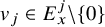 $v_j\in E_x^j\backslash \{0\}$
, we have for n large enough,
$v_j\in E_x^j\backslash \{0\}$
, we have for n large enough,
 $$ \begin{align*}\|A_n(x)v_j\|>\|A_n(x)v_{j+1}\|.\end{align*} $$
Oseledets decomposition is a priori only measurable, however if an invariant decomposition
 ${\mathbb {C}}^m=E_x^1\oplus E_x^2\oplus \cdots \oplus E_x^\ell $
is dominated, then
${\mathbb {C}}^m=E_x^1\oplus E_x^2\oplus \cdots \oplus E_x^\ell $
is dominated, then
 $E_x^j$
depends continuously on x [Reference Bonatti, Diaz and Viana20].
$E_x^j$
depends continuously on x [Reference Bonatti, Diaz and Viana20].
A cocycle
 $(\alpha ,A)$
is called k-dominated (for some
$(\alpha ,A)$
is called k-dominated (for some
 $1\leq k\leq m-1$
) if there exists a dominated decomposition
$1\leq k\leq m-1$
) if there exists a dominated decomposition
 ${\mathbb {C}}^m=E^+ \oplus E^- $
with
${\mathbb {C}}^m=E^+ \oplus E^- $
with
 $\dim E^+ = k.$
If
$\dim E^+ = k.$
If
 $\alpha \in {\mathbb {R}}\backslash {\mathbb {Q}}$
, then it follows from the definitions that the Oseledets splitting is dominated if and only if
$\alpha \in {\mathbb {R}}\backslash {\mathbb {Q}}$
, then it follows from the definitions that the Oseledets splitting is dominated if and only if
 $(\alpha ,A)$
is k-dominated for each k such that
$(\alpha ,A)$
is k-dominated for each k such that
 $L_k(\alpha ,A)> L_{k+1}(\alpha ,A)$
.
$L_k(\alpha ,A)> L_{k+1}(\alpha ,A)$
.
4.3 Global theory of one-frequency quasiperiodic cocycles
We briefly introduce the global theory of one-frequency quasiperiodic cocycles, first developed for
 $SL(2,{\mathbb {C}})$
-cocycles [Reference Avila3], and later generalized to any
$SL(2,{\mathbb {C}})$
-cocycles [Reference Avila3], and later generalized to any
 $\mathrm {M}_m({\mathbb {C}})$
-cocycles [Reference Avila, Jitomirskaya and Sadel11]. The most important concept of the global theory is the acceleration. If
$\mathrm {M}_m({\mathbb {C}})$
-cocycles [Reference Avila, Jitomirskaya and Sadel11]. The most important concept of the global theory is the acceleration. If
 $A\in C^{\omega }({\mathbb {T}},\mathrm {M}_m({\mathbb {C}}))$
admits a holomorphic extension to
$A\in C^{\omega }({\mathbb {T}},\mathrm {M}_m({\mathbb {C}}))$
admits a holomorphic extension to
 $|\Im z|<\delta $
, then for
$|\Im z|<\delta $
, then for
 $|{\varepsilon }|<\delta $
we can define
$|{\varepsilon }|<\delta $
we can define
 $A_{\varepsilon }\in C^{\omega }({\mathbb {T}},M_m({\mathbb {C}}))$
by
$A_{\varepsilon }\in C^{\omega }({\mathbb {T}},M_m({\mathbb {C}}))$
by
 $A_{\varepsilon }(x)=A(x+i{\varepsilon })$
. The accelerations of
$A_{\varepsilon }(x)=A(x+i{\varepsilon })$
. The accelerations of
 $(\alpha ,A)$
is defined as
$(\alpha ,A)$
is defined as
 $$ \begin{align*}\omega^k(\alpha,A)=\lim\limits_{{\varepsilon}\rightarrow 0^+}\frac{1}{2\pi{\varepsilon}}(L^k(\alpha,A_{\varepsilon})-L^k(\alpha,A)), \qquad \omega_k(\alpha,A)= \omega^k(\alpha,A)-\omega^{k-1}(\alpha,A). \end{align*} $$
The key ingredient to the global theory is that the acceleration is quantized.
Theorem 4.2 [Reference Avila3, Reference Avila, Jitomirskaya and Sadel11].
There exist
 $1\leq l\leq m$
,
$1\leq l\leq m$
,
 $l\in {\mathbb {N}}$
, such that
$l\in {\mathbb {N}}$
, such that
 $l\omega ^k$
and
$l\omega ^k$
and
 $l \omega _k$
are integers. In particular, if
$l \omega _k$
are integers. In particular, if
 $A\in C^\omega ({\mathbb {T}}, SL(2,{\mathbb {C}}))$
, then
$A\in C^\omega ({\mathbb {T}}, SL(2,{\mathbb {C}}))$
, then
 $\omega ^1(\alpha ,A)$
is an integer.
$\omega ^1(\alpha ,A)$
is an integer.
Remark 4.3. If
 $L_j(\alpha ,A)>L_{j+1}(\alpha ,A)$
, then
$L_j(\alpha ,A)>L_{j+1}(\alpha ,A)$
, then
 $\omega ^j(\alpha ,A)$
is an integer. This is contained in the proof of Theorem 1.4 in [Reference Avila, Jitomirskaya and Sadel11], see also footnote 17 in [Reference Avila, Jitomirskaya and Sadel11].
$\omega ^j(\alpha ,A)$
is an integer. This is contained in the proof of Theorem 1.4 in [Reference Avila, Jitomirskaya and Sadel11], see also footnote 17 in [Reference Avila, Jitomirskaya and Sadel11].
By subharmonicity, we know that
 $L^k(\alpha ,A(\cdot +i{\varepsilon }))$
is a convex function of
$L^k(\alpha ,A(\cdot +i{\varepsilon }))$
is a convex function of
 ${\varepsilon } $
in a neighborhood of
${\varepsilon } $
in a neighborhood of
 $0$
, unless it is identically equal to
$0$
, unless it is identically equal to
 $-\infty $
. We say that
$-\infty $
. We say that
 $(\alpha ,A)$
is k-regular if
$(\alpha ,A)$
is k-regular if
 ${\varepsilon }\rightarrow L^k(\alpha ,A(\cdot +i{\varepsilon }))$
is an affine function of
${\varepsilon }\rightarrow L^k(\alpha ,A(\cdot +i{\varepsilon }))$
is an affine function of
 ${\varepsilon }$
in a neighborhood of
${\varepsilon }$
in a neighborhood of
 $0$
. In general, one can relate regularity and dominated splitting as follows.
$0$
. In general, one can relate regularity and dominated splitting as follows.
Theorem 4.3 [Reference Avila3, Reference Avila, Jitomirskaya and Sadel11].
Let
 $\alpha \in {\mathbb {R}}\backslash {\mathbb {Q}}$
and
$\alpha \in {\mathbb {R}}\backslash {\mathbb {Q}}$
and
 $A\in C^\omega ({\mathbb {T}},M_m({\mathbb {C}}))$
. If
$A\in C^\omega ({\mathbb {T}},M_m({\mathbb {C}}))$
. If
 $1\leq j\leq m-1$
is such that
$1\leq j\leq m-1$
is such that
 $L_j(\alpha ,A)>L_{j+1}(\alpha ,A)$
, then
$L_j(\alpha ,A)>L_{j+1}(\alpha ,A)$
, then
 $(\alpha ,A)$
is j-regular if and only if
$(\alpha ,A)$
is j-regular if and only if
 $(\alpha ,A)$
is j-dominated. In particular, if
$(\alpha ,A)$
is j-dominated. In particular, if
 $A\in C^\omega ({\mathbb {T}}, SL(2,{\mathbb {C}}))$
with
$A\in C^\omega ({\mathbb {T}}, SL(2,{\mathbb {C}}))$
with
 $L(\alpha ,A)>0$
, then
$L(\alpha ,A)>0$
, then
 $(\alpha ,A)$
is
$(\alpha ,A)$
is
 $1$
-regular (or regular) if and only if
$1$
-regular (or regular) if and only if
 $(\alpha ,A)$
is uniformly hyperbolic.
$(\alpha ,A)$
is uniformly hyperbolic.
4.4 Schrödinger operators and Schrödinger cocycles
Let
 $(\Omega ,\tilde {d})$
be a compact metric space with distance
$(\Omega ,\tilde {d})$
be a compact metric space with distance
 $\tilde {d}$
,
$\tilde {d}$
,
 $T:\Omega \rightarrow \Omega $
a homeomorphism, and
$T:\Omega \rightarrow \Omega $
a homeomorphism, and
 $V:\Omega \rightarrow {\mathbb {C}}$
a complex-valued continuous function.
$V:\Omega \rightarrow {\mathbb {C}}$
a complex-valued continuous function.
 $(\Omega ,T)$
is said to be minimal if each T-orbit is dense. We consider the following complex-valued dynamically defined Schrödinger operators:
$(\Omega ,T)$
is said to be minimal if each T-orbit is dense. We consider the following complex-valued dynamically defined Schrödinger operators:
 $$ \begin{align} (H_{x}u)_n=u_{n+1}+u_{n-1}+V(T^nx)u_n,\ \ n\in{\mathbb{Z}}, \end{align} $$
and denote by
 $\Sigma _x$
the spectrum of
$\Sigma _x$
the spectrum of
 $H_{x}$
. We have the following:
$H_{x}$
. We have the following:
Lemma 4.1. There is some
 $\Sigma \subset {\mathbb {C}}$
such that
$\Sigma \subset {\mathbb {C}}$
such that
 $\Sigma _x=\Sigma $
for all
$\Sigma _x=\Sigma $
for all
 $x\in \Omega $
.
$x\in \Omega $
.
Remark 4.4. This is a standard fact for real-valued V (so self-adjoint H). We provide here a brief argument that does not require self-adjointness.
Proof. We only need to prove that for any
 $x,y\in \Omega $
,
$x,y\in \Omega $
,
 $\Sigma _x=\Sigma _y$
. Assume
$\Sigma _x=\Sigma _y$
. Assume
 $E\notin \Sigma _x$
, that is
$E\notin \Sigma _x$
, that is
 $(H_x-E)^{-1}$
exists and is bounded. Since
$(H_x-E)^{-1}$
exists and is bounded. Since
 $(\Omega ,T)$
is minimal, there is a subsequence
$(\Omega ,T)$
is minimal, there is a subsequence
 $\{n_i\}_{i=1}^\infty $
such that
$\{n_i\}_{i=1}^\infty $
such that
 $T^{n_i}y\rightarrow x$
. Since
$T^{n_i}y\rightarrow x$
. Since
 $\Omega $
is compact, T is uniformly continuous which implies that
$\Omega $
is compact, T is uniformly continuous which implies that
 $H_{T^{n_i}y}\rightarrow H_x$
in operator norm. Hence
$H_{T^{n_i}y}\rightarrow H_x$
in operator norm. Hence
 $(H_{T^{n_i}y}-E)^{-1}$
exists and is bounded for i sufficiently large, which implies
$(H_{T^{n_i}y}-E)^{-1}$
exists and is bounded for i sufficiently large, which implies
 $E\notin \Sigma _{T^{n_i}y}$
for i sufficiently large. Since
$E\notin \Sigma _{T^{n_i}y}$
for i sufficiently large. Since
 $H_y$
and
$H_y$
and
 $H_{T^{n_i}y}$
are unitarily equivalent, we have
$H_{T^{n_i}y}$
are unitarily equivalent, we have
 $E\notin \Sigma _{y}$
, thus
$E\notin \Sigma _{y}$
, thus
 $\Sigma _y\subset \Sigma _x$
. Similarly,
$\Sigma _y\subset \Sigma _x$
. Similarly,
 $\Sigma _x\subset \Sigma _y$
.
$\Sigma _x\subset \Sigma _y$
.
Note that any formal solution
 $u=(u_n)_{n \in {\mathbb {Z}}}$
of
$u=(u_n)_{n \in {\mathbb {Z}}}$
of
 $H_{x}u=E u$
satisfies
$H_{x}u=E u$
satisfies
 $$ \begin{align*} \begin{pmatrix}u_{n+1}\\u_n\end{pmatrix}= A_E(T^n x) \begin{pmatrix}u_{n}\\u_{n-1}\end{pmatrix},\quad \forall \ n \in {\mathbb{Z}}, \end{align*} $$
where
 $$ \begin{align*}A_E(x):= \begin{pmatrix}E-V(x) & -1\\1 & 0\end{pmatrix}, \quad E\in{\mathbb{R}}. \end{align*} $$
We call
 $(T,A_E)$
Schrödinger cocycles. The spectrum
$(T,A_E)$
Schrödinger cocycles. The spectrum
 $\Sigma $
is closely related to the dynamical behavior of the Schrödinger cocycle
$\Sigma $
is closely related to the dynamical behavior of the Schrödinger cocycle
 $(T,A_E)$
. In the self-adjoint case, that is, the potential V is real valued, then by the celebrated Johnson’s theorem [Reference Jonhnson61],
$(T,A_E)$
. In the self-adjoint case, that is, the potential V is real valued, then by the celebrated Johnson’s theorem [Reference Jonhnson61],
 $E\notin \Sigma $
if and only if
$E\notin \Sigma $
if and only if
 $(T,A_E)$
is uniformly hyperbolic. It turns out that it is not difficult to extend Johnson’s theorem [Reference Jonhnson61] to the non-self-adjoint case. We will give a proof in the appendix.
$(T,A_E)$
is uniformly hyperbolic. It turns out that it is not difficult to extend Johnson’s theorem [Reference Jonhnson61] to the non-self-adjoint case. We will give a proof in the appendix.
Theorem 4.4. Suppose that
 $V:\Omega \rightarrow {\mathbb {C}}$
is a complex-valued continuous function and
$V:\Omega \rightarrow {\mathbb {C}}$
is a complex-valued continuous function and
 $(\Omega ,T)$
is minimal, then
$(\Omega ,T)$
is minimal, then
 $E\notin \Sigma $
if and only if
$E\notin \Sigma $
if and only if
 $(T,A_E)$
is uniformly hyperbolic.
$(T,A_E)$
is uniformly hyperbolic.
In this paper, we are mainly interested in the following complex-valued quasiperiodic Schrödinger operators
 $$ \begin{align*}(H_{V,x+i{\varepsilon},\alpha}u)_n=u_{n+1}+u_{n-1}+V(x+i{\varepsilon}+n\alpha)u_n, \end{align*} $$
and corresponding Schrödinger cocycles
 $(\alpha ,A_E(\cdot +i{\varepsilon }))$
. Throughout the paper, we will denote
$(\alpha ,A_E(\cdot +i{\varepsilon }))$
. Throughout the paper, we will denote
 $L_{\varepsilon }(E)=L(\alpha ,A_E(\cdot +i{\varepsilon }))$
for short.
$L_{\varepsilon }(E)=L(\alpha ,A_E(\cdot +i{\varepsilon }))$
for short.
4.5 Quasiperiodic Schrödinger operators on the strip
We recall that quasiperiodic finite-range operator
 $$ \begin{align*} (\widehat{H}_{V,\theta,\alpha}u)(n)=\sum\limits_{k=-d}^{d} V_k u_{n+k}+2\cos 2\pi (\theta+n\alpha)u_n, \ \ n\in{\mathbb{Z}}. \end{align*} $$
naturally induces a quasiperiodic cocycle
 $(\alpha ,\widehat {A}_{E})$
where
$(\alpha ,\widehat {A}_{E})$
where
 $$ \begin{align*} \widehat{A}_{E}(\theta)=\frac{1}{V_d}\begin{pmatrix}\begin{smallmatrix}-V_{d-1}&\cdots&-V_1&E-2\cos2\pi(\theta)-V_0&-V_{-1}&\cdots&-V_{-d+1}&-V_{-d}\\V_d& \\& & \\& & & \\\\\\& & &\ddots&\\\\\\& & & & \\& & & & & \\& & & & & &V_{d}&\end{smallmatrix}\end{pmatrix}. \end{align*} $$
We can write it as a second order
 $2d$
-dimensional difference equation by introducing the auxiliary variables
$2d$
-dimensional difference equation by introducing the auxiliary variables
 $$ \begin{align*}\vec{u}_k=(u_{dk+d-1}\ \ \cdots\ \ u_{dk+1}\ \ u_{dk})^T \end{align*} $$
for
 $k\in {\mathbb {Z}}$
. It is easy to check that
$k\in {\mathbb {Z}}$
. It is easy to check that
 $(\vec {u}_k)_k$
satisfies
$(\vec {u}_k)_k$
satisfies
 $$ \begin{align} C\vec{u}_{k+1}+B(\theta_{dk})\vec{u}_k+C^*\vec{u}_{k-1}=E\vec{u}_k, \end{align} $$
where
 $$ \begin{align*} C=\begin{pmatrix}V_d&\cdots&V_1\\0&\ddots&\vdots\\0&0&V_d\end{pmatrix}, \end{align*} $$
 $C^*$
is the transposed and conjugated matrix of C, and
$C^*$
is the transposed and conjugated matrix of C, and
 $B(\theta )$
is the Hermitian matrix
$B(\theta )$
is the Hermitian matrix
 $$ \begin{align} B(\theta)=\begin{pmatrix}2\cos 2\pi (\theta_{d-1})&V_{-1}&\cdots&V_{-d+1}\\V_1&\ddots&\ddots&\vdots\\\vdots&\ddots&2\cos 2 \pi (\theta_1)&V_{-1}\\V_{d-1}&\cdots&V_1&2\cos2 \pi(\theta)\end{pmatrix} \end{align} $$
where
 $\theta _j=\theta +j\alpha $
. Note that equation (4.3) is an eigenequation of the following Schrödinger operator on the strip
$\theta _j=\theta +j\alpha $
. Note that equation (4.3) is an eigenequation of the following Schrödinger operator on the strip
 $$ \begin{align*}(H_{C,B,\theta,d\alpha}\vec{u})_k=C\vec{u}_{k+1}+B(T^k\theta)\vec{u}_k+C^*\vec{u}_{k-1}, \end{align*} $$
acting on
 $\ell ^2({\mathbb {Z}},{\mathbb {C}}^d)$
, which is an ergodic operator with the dynamics given by
$\ell ^2({\mathbb {Z}},{\mathbb {C}}^d)$
, which is an ergodic operator with the dynamics given by
 $T\theta =\theta +d\alpha $
.
$T\theta =\theta +d\alpha $
.
To obtain a first order system and the corresponding linear skew product we use the fact that C is invertible (since
 $V_d\neq 0$
because the degree of V is exactly d) and write
$V_d\neq 0$
because the degree of V is exactly d) and write
 $$ \begin{align*} \begin{pmatrix}\vec{u}_{k+1}\\\vec{u}_k\end{pmatrix}=\begin{pmatrix}C^{-1}(EI-B(T^k\theta))& -C^{-1}C^*\\I_d&O_d\end{pmatrix}\begin{pmatrix}\vec{u}_k\\\vec{u}_{k-1}\end{pmatrix} \end{align*} $$
where
 $I_d$
and
$I_d$
and
 $O_d$
are the d-dimensional identity and zero matrices, respectively. Denote
$O_d$
are the d-dimensional identity and zero matrices, respectively. Denote
 $$ \begin{align} \widehat{A}_{d,E}(\theta)=\begin{pmatrix}C^{-1}(EI-B(\theta))& -C^{-1}C^*\\I_d&O_d\end{pmatrix} \end{align} $$
An important ingredient for our results is the complex symplectic structure
 $$ \begin{align*} \Omega=\begin{pmatrix}0&-C^*\\C&0\end{pmatrix} \end{align*} $$
which satisfies
 $\Omega ^*=-\Omega $
, and the fact that our Schrödinger skew-products
$\Omega ^*=-\Omega $
, and the fact that our Schrödinger skew-products
 $(d\alpha ,\widehat {A}_{d,E})$
are complex symplectic for real E with respect to
$(d\alpha ,\widehat {A}_{d,E})$
are complex symplectic for real E with respect to
 $\Omega $
. However, if E is complex, then
$\Omega $
. However, if E is complex, then
 $ (d\alpha ,\widehat {A}_{d,E})$
are not complex symplectic anymore. For more details, see [Reference Haro and Puig46].
$ (d\alpha ,\widehat {A}_{d,E})$
are not complex symplectic anymore. For more details, see [Reference Haro and Puig46].
We denote
 $\gamma _{i}(E)=\frac {L_i(\alpha ,\widehat {A}_{E})}{2\pi }$
for
$\gamma _{i}(E)=\frac {L_i(\alpha ,\widehat {A}_{E})}{2\pi }$
for
 $1\leq i\leq d$
for short. Then using the Kotani-Simon [Reference Kotani and Simon63] version of the Thouless formula for the strip, one can prove the following beautiful Haro-Puig’s formula
$1\leq i\leq d$
for short. Then using the Kotani-Simon [Reference Kotani and Simon63] version of the Thouless formula for the strip, one can prove the following beautiful Haro-Puig’s formula
Theorem 4.5 [Reference Haro and Puig46].
For any
 $E\in {\mathbb {C}}$
, we have
$E\in {\mathbb {C}}$
, we have
 $$ \begin{align} L(E)=2\pi\left(\sum\limits_{i=1}^{d} \gamma_i(E)\right)+\ln |V_{d}|. \end{align} $$
5 Green’s function of finite-range Schrödinger operator
In this section, we explore the M matrix and Green’s matrix for the following Schrödinger operators on the strip
 $$ \begin{align} (H_{C,B,\theta,d\alpha}\vec{u})_k=C\vec{u}_{k+1}+B(T^k\theta)\vec{u}_k+C^*\vec{u}_{k-1}, \end{align} $$
where
 $T^k\theta =\theta +kd\alpha $
.
$T^k\theta =\theta +kd\alpha $
.
5.1 The M matrix and the Green’s matrix
In the following,
 ${\mathbb {C}}_+$
will denote
${\mathbb {C}}_+$
will denote
 $\{E\in {\mathbb {C}}|\Im E>0\}$
. For any energy in
$\{E\in {\mathbb {C}}|\Im E>0\}$
. For any energy in
 ${\mathbb {C}}_+$
, one can define the M matrix and Green’s matrix with the help of the following result:
${\mathbb {C}}_+$
, one can define the M matrix and Green’s matrix with the help of the following result:
Lemma 5.1 [Reference Haro and Puig46],[Reference Kotani and Simon63].
For any
 $E\in {\mathbb {C}}_+$
, there exist unique sequences of
$E\in {\mathbb {C}}_+$
, there exist unique sequences of
 $d\times d$
matrix valued functions
$d\times d$
matrix valued functions
 $\{F_{\pm }(k,\theta ,E)\}_{k\in {\mathbb {Z}}}$
that satisfy the following properties:
$\{F_{\pm }(k,\theta ,E)\}_{k\in {\mathbb {Z}}}$
that satisfy the following properties:
-
1.
$F_\pm (0,\theta ,E)=I_d,$
-
2.
$$ \begin{align*}C^*F_{\pm}(k-1,\theta,E)+CF_\pm(k+1,\theta,E)+B(T^k\theta)F_\pm(k,\theta,E)=EF_\pm(k,\theta,E), \end{align*} $$
-
3.
$$ \begin{align*}\sum\limits_{k=0}^\infty\|F_+(k,\theta,E)\|^2<\infty, \ \ \sum\limits_{k=-\infty}^{0}\|F_-(k,\theta,E)\|^2<\infty. \end{align*} $$


Once we have
 $F_{\pm }(k,\theta ,E)$
, we can define the M matrices
$F_{\pm }(k,\theta ,E)$
, we can define the M matrices
 $$ \begin{align*}M_+(\theta,E)=-F_+(1,\theta,E), \end{align*} $$
 $$ \begin{align*}M_-(\theta,E)=-F_-(-1,\theta,E), \end{align*} $$
as in [Reference Kotani and Simon63], and note that the M matrices satisfy the following Riccati equations.
Lemma 5.2. For any
 $n\in {\mathbb {Z}}$
, we have
$n\in {\mathbb {Z}}$
, we have
 $$ \begin{align} CM_+(T^{n}\theta,E)+C^*M_+^{-1}(T^{n-1}\theta,E)+(E-B(T^n\theta))=0. \end{align} $$
 $$ \begin{align} C^*M_-(T^n\theta,E)+CM_-^{-1}(T^{n+1}\theta,E)+(E-B(T^n\theta))=0. \end{align} $$
Proof. We only prove (5.2), since (5.3) can be proved similarly. Note that
 $F_+(n,\theta ,E)$
satisfies
$F_+(n,\theta ,E)$
satisfies
 $$ \begin{align*}C^*F_+(n-1,\theta,E)+CF_+(n+1,\theta,E)+B(T^n\theta)F_+(n,\theta,E)=EF_+(n,\theta,E), \end{align*} $$
and by the fact that
 $$ \begin{align*}F_+(m+n,\theta,E)= F_+(m, T^n \theta,E)F_+(n,\theta,E),\end{align*} $$
we have
 $$ \begin{align*}C^*M^{-1}_+(T^{n-1}\theta,E)+CM_+(T^n\theta,E)+(E-B(T^n\theta))=0.\\[-34pt] \end{align*} $$
Similarly as in [Reference Kotani and Simon63], one can define the Green’s matrix as
 $$ \begin{align*}G(\theta,E)= \langle \vec{\delta}_0,(H_{C,B,\theta,d\alpha}-E)^{-1}\vec{\delta}_0\rangle, \end{align*} $$
where
 $$ \begin{align*}\vec{\delta}_j(n)= \begin{cases} 0& n\neq j\\ I_d &n=j \end{cases}. \end{align*} $$
The Green’s matrix can be expressed as the following:
Lemma 5.3. For any
 $E\in {\mathbb {C}}_+$
, we have
$E\in {\mathbb {C}}_+$
, we have
 $$ \begin{align*} G(\theta,E)=(-CM_+(\theta,E)-C^*M_-(\theta,E)+B(\theta)-E)^{-1} \end{align*} $$
Proof. It is easy to check that
 $$ \begin{align*} &\langle \vec{\delta}_n,(H_{C,B,\theta,d\alpha}-E)^{-1}\vec{\delta}_0\rangle \\ =&\begin{cases} F_+(n,\theta,E)(CF_+(1,\theta,E)+C^*F_-(-1,\theta,E)+B(\theta)-E)^{-1}& n\geq 0\\ F_-(n,\theta,E)(CF_+(1,\theta,E)+C^*F_-(-1,\theta,E)+B(\theta)-E)^{-1}& n< 0 \end{cases}.\\[-38pt] \end{align*} $$
The following Lemma gives the relation between the M matrix and the Green’s matrix.
Lemma 5.4. For any
 $E\in {\mathbb {C}}_+$
, the following relation holds:
$E\in {\mathbb {C}}_+$
, the following relation holds:
 $$ \begin{align} \nonumber G(\theta,E)&=(-CM_+(\theta,E)+CM^{-1}_-(T\theta,E))^{-1}, \\ \nonumber G(T\theta,E)&= (C^*M_+^{-1}(\theta,E)-C^*M_-(T\theta,E))^{-1},\\ G(\theta,E)CM^{-1}_-(T\theta,E) &= M_-(T\theta,E)G(T\theta,E) C^* + I_d. \end{align} $$
Proof. By Lemma 5.3, (5.2) and (5.3), one has
 $$ \begin{align*} G(T\theta,E)&=(-CM_+(T\theta,E)-C^*M_-(T\theta,E)+B(T\theta)-E)^{-1}\\ \nonumber &=(C^*M_+^{-1}(\theta,E)-C^*M_-(T\theta,E))^{-1}. \end{align*} $$
 $$ \begin{align*} G(\theta,E)&=(-CM_+(\theta,E)-C^*M_-(\theta,E)+B(\theta)-E)^{-1}\\ \nonumber &=(-CM_+(\theta,E)+CM^{-1}_-(T\theta,E))^{-1}. \end{align*} $$
Consequently, we have the following
 $$ \begin{align*} G(\theta,E)CM^{-1}_-(T\theta,E) &=(I_d - M_-(T\theta,E)M_+(\theta,E))^{-1}\\ \nonumber &=M_+^{-1}(\theta,E)(M_+^{-1}(\theta,E)- M_-(T\theta,E))^{-1}\\ \nonumber &=M_-(T\theta,E)(M^{-1}_+(\theta,E)-M_-(T\theta,E))^{-1} + I_d\\ \nonumber &= M_-(T\theta,E)G(T\theta,E) C^* + I_d.\\[-38pt] \end{align*} $$
5.2 A dynamical consequence: dominated splitting
For any
 $E\in {\mathbb {C}}$
, we group
$E\in {\mathbb {C}}$
, we group
 $\{\gamma _i(E)\}_{i=1}^d$
as
$\{\gamma _i(E)\}_{i=1}^d$
as
 $\gamma _{n_1}, \cdots , \gamma _{n_\ell }$
with multiplicities
$\gamma _{n_1}, \cdots , \gamma _{n_\ell }$
with multiplicities
 $\{n_{i}-n_{i-1}\}_{i=1}^\ell $
respectively, where
$\{n_{i}-n_{i-1}\}_{i=1}^\ell $
respectively, where
 $n_0=0$
and we assume that
$n_0=0$
and we assume that
 $$ \begin{align*}\gamma_{n_1}>\gamma_{n_2}>\cdots>\gamma_{n_{\ell}}\geq 0. \end{align*} $$
Note that
 $(d\alpha ,\widehat {A}_{d,E})=(\alpha ,\widehat {A}_E)^d$
is the d-th iteration of
$(d\alpha ,\widehat {A}_{d,E})=(\alpha ,\widehat {A}_E)^d$
is the d-th iteration of
 $(\alpha ,\widehat {A}_{E}),$
we have
$(\alpha ,\widehat {A}_{E}),$
we have
 $L_i(d\alpha ,\widehat {A}_{d,E})=2\pi d\gamma _i(E)$
. Hence
$L_i(d\alpha ,\widehat {A}_{d,E})=2\pi d\gamma _i(E)$
. Hence
 $\{L_{n_i}(d\alpha ,\widehat {A}_{d,E})\}_{i=1}^\ell $
are the distinct Lyapunov exponents of
$\{L_{n_i}(d\alpha ,\widehat {A}_{d,E})\}_{i=1}^\ell $
are the distinct Lyapunov exponents of
 $(d\alpha ,\widehat {A}_{d,E})$
. Note that we always have
$(d\alpha ,\widehat {A}_{d,E})$
. Note that we always have
 $$ \begin{align*}n_{\ell(E)}(E)=d.\end{align*} $$
Indeed, if
 $E\in {\mathbb {R}}$
,
$E\in {\mathbb {R}}$
,
 $(d\alpha ,\widehat {A}_{d,E})$
are complex symplectic, thus by Remark 4.2, the Lyapunov exponents of
$(d\alpha ,\widehat {A}_{d,E})$
are complex symplectic, thus by Remark 4.2, the Lyapunov exponents of
 $(\alpha ,\widehat {A}_{E})$
come in pairs
$(\alpha ,\widehat {A}_{E})$
come in pairs
 $\{\pm \gamma _i(E)\}_{i=1}^d$
. If
$\{\pm \gamma _i(E)\}_{i=1}^d$
. If
 $E\in {\mathbb {C}} \backslash {\mathbb {R}}$
,
$E\in {\mathbb {C}} \backslash {\mathbb {R}}$
,
 $(d\alpha ,\widehat {A}_{d,E})$
is uniformly hyperbolic [Reference Haro and Puig46], thus
$(d\alpha ,\widehat {A}_{d,E})$
is uniformly hyperbolic [Reference Haro and Puig46], thus
 $L_d(d\alpha ,\widehat {A}_{d,E})>0$
. A key observation of our proof is the following:
$L_d(d\alpha ,\widehat {A}_{d,E})>0$
. A key observation of our proof is the following:
Proposition 5.1. For
 $E\in {\mathbb {C}}_+$
, the cocycle
$E\in {\mathbb {C}}_+$
, the cocycle
 $(d\alpha ,\widehat {A}_{d,E})$
is
$(d\alpha ,\widehat {A}_{d,E})$
is
 $n_i$
-dominated for
$n_i$
-dominated for
 $1\leq i\leq \ell $
.
$1\leq i\leq \ell $
.
Proof. We divide the proof into two cases:
Case 1:
 $\mathbf {i=\ell }$
. Since
$\mathbf {i=\ell }$
. Since
 $E\in {\mathbb {C}}_+$
, we have that
$E\in {\mathbb {C}}_+$
, we have that
 $(d\alpha ,\widehat {A}_{d,E})$
is uniformly hyperbolic [Reference Haro and Puig46], which implies that
$(d\alpha ,\widehat {A}_{d,E})$
is uniformly hyperbolic [Reference Haro and Puig46], which implies that
 $n_{\ell }=d$
and
$n_{\ell }=d$
and
 $(d\alpha ,\widehat {A}_{d,E})$
is d-dominated.
$(d\alpha ,\widehat {A}_{d,E})$
is d-dominated.
Case 2:
 $\mathbf {1\leq i\leq \ell -1}$
. Recall that
$\mathbf {1\leq i\leq \ell -1}$
. Recall that
 $$ \begin{align*} \widehat{A}_{d,E}(\theta)=\begin{pmatrix}C^{-1}(EI-B(\theta))& -C^{-1}C^*\\I_d&O_d\end{pmatrix} \end{align*} $$
where
 $$ \begin{align*} B(\theta)=\begin{pmatrix}2\cos(\theta_{d-1})&V_{-1}&\cdots&V_{-d+1}\\V_1&\ddots&\ddots&\vdots\\\vdots&\ddots&2\cos(\theta_1)&V_{-1}\\V_{d-1}&\cdots&V_1&2\cos(\theta)\end{pmatrix}. \end{align*} $$
Thus if we let
 $\left (\ell _{ij}\right )_{1\leq i,j\leq d}=(\widehat {A}_{d,E})_n(\theta )=\widehat {A}_{d,E}(\theta +(n-1)\alpha )\cdots \widehat {A}_{d,E}(\theta +\alpha )\widehat {A}_{d,E}(\theta )$
, then it is easy to check that each
$\left (\ell _{ij}\right )_{1\leq i,j\leq d}=(\widehat {A}_{d,E})_n(\theta )=\widehat {A}_{d,E}(\theta +(n-1)\alpha )\cdots \widehat {A}_{d,E}(\theta +\alpha )\widehat {A}_{d,E}(\theta )$
, then it is easy to check that each
 $\ell _{ij}$
is a polynomial of
$\ell _{ij}$
is a polynomial of
 $\cos 2\pi (\theta )$
with degree
$\cos 2\pi (\theta )$
with degree
 $\leq n$
. Similarly, if we let
$\leq n$
. Similarly, if we let
 $L_{ij}$
be the
$L_{ij}$
be the
 $ij$
-th entry of
$ij$
-th entry of
 $\Lambda ^{n_i}(\widehat {A}_{d,E})_n(\theta )$
, by the definition of wedge,
$\Lambda ^{n_i}(\widehat {A}_{d,E})_n(\theta )$
, by the definition of wedge,
 $L_{ij}$
is a polynomial of
$L_{ij}$
is a polynomial of
 $\cos 2\pi (\theta )$
with degree
$\cos 2\pi (\theta )$
with degree
 $\leq nn_i$
. Hence one can compute
$\leq nn_i$
. Hence one can compute
 $$ \begin{align*} &|\omega^{n_i}(d\alpha,\widehat{A}_{d,E})|=\left|\lim\limits_{{\varepsilon}\rightarrow 0^+}\frac{1}{2\pi{\varepsilon}}(L^{n_i}(d\alpha,\widehat{A}_{d,E}(\cdot+i{\varepsilon}))-L^{n_i}(d\alpha,\widehat{A}_{d,E})\right|\\ &=\frac{1}{2\pi}\left|\lim\limits_{n\rightarrow \infty}\frac{1}{n}\int_{{\mathbb{T}}}\ln(\|\Lambda^{n_i}(\widehat{A}_{d,E})_n(\theta+i{\varepsilon})\|)d\theta-\lim\limits_{n\rightarrow \infty}\frac{1}{n}\int_{{\mathbb{T}}}\ln(\|\Lambda^{n_i}(\widehat{A}_{d,E})_n(\theta)\|)d\theta\right| \leq n_i. \end{align*} $$
It follows that
 $$ \begin{align*}|\omega^{n_i}(\alpha,\widehat{A}_{E})|=\left|\frac{\omega^{n_i}(d\alpha,\widehat{A}_{d,E})}{d}\right|\leq \frac{n_i}{d}<1. \end{align*} $$
On the other hand, since
 $\gamma _{n_i}(E)>\gamma _{n_{i}+1}(E)$
, by Remark 4.3,
$\gamma _{n_i}(E)>\gamma _{n_{i}+1}(E)$
, by Remark 4.3,
 $\omega ^{n_i}(\alpha ,\widehat {A}_{E})$
is an integer. Together with the fact that
$\omega ^{n_i}(\alpha ,\widehat {A}_{E})$
is an integer. Together with the fact that
 $|\omega ^{n _i}(\alpha ,\widehat {A}_{E})|$
is strictly smaller than
$|\omega ^{n _i}(\alpha ,\widehat {A}_{E})|$
is strictly smaller than
 $1$
, we have
$1$
, we have
 $\omega ^{n_i}(\alpha ,\widehat {A}_{E})=0$
. This implies that
$\omega ^{n_i}(\alpha ,\widehat {A}_{E})=0$
. This implies that
 $$ \begin{align*}L^{n_i}(\alpha,\widehat{A}_{E}(\cdot+i{\varepsilon}))=L^{n_i}(\alpha,\widehat{A}_{E}) \end{align*} $$
for
 ${\varepsilon }>0$
which is sufficiently small. Similar argument works for
${\varepsilon }>0$
which is sufficiently small. Similar argument works for
 ${\varepsilon }<0$
which is also sufficiently small. This means
${\varepsilon }<0$
which is also sufficiently small. This means
 $(\alpha ,\widehat {A}_{E})$
is
$(\alpha ,\widehat {A}_{E})$
is
 $n_i$
-regular. Notice that
$n_i$
-regular. Notice that
 $$ \begin{align*}dL^{n_i}(\alpha,\widehat{A}_{E}(\cdot+i{\varepsilon}))=L^{n_i}(d\alpha,\widehat{A}_{d,E}(\cdot+i{\varepsilon})). \end{align*} $$
so
 $(\alpha ,\widehat {A}_{E})$
is
$(\alpha ,\widehat {A}_{E})$
is
 $n_i$
-regular if and only if
$n_i$
-regular if and only if
 $(d\alpha ,\widehat {A}_{d,E})$
is
$(d\alpha ,\widehat {A}_{d,E})$
is
 $n_i$
-regular. Hence
$n_i$
-regular. Hence
 $(d\alpha ,\widehat {A}_{d,E})$
is
$(d\alpha ,\widehat {A}_{d,E})$
is
 $n_i$
-dominated by Theorem 4.3.
$n_i$
-dominated by Theorem 4.3.
Corollary 5.1. Assume
 $\alpha \in {\mathbb {R}}\backslash {\mathbb {Q}}, E\in {\mathbb {R}}$
, and
$\alpha \in {\mathbb {R}}\backslash {\mathbb {Q}}, E\in {\mathbb {R}}$
, and
 $\gamma _d=0.$
Then
$\gamma _d=0.$
Then
 $(d\alpha ,\widehat {A}_{d,E})$
is partially hyperbolic with center of dimension
$(d\alpha ,\widehat {A}_{d,E})$
is partially hyperbolic with center of dimension
 $2(n_\ell -n_{\ell -1})$
.
$2(n_\ell -n_{\ell -1})$
.
Proof. For any
 $E\in {\mathbb {R}}$
, by the same argument as in Proposition 5.1,
$E\in {\mathbb {R}}$
, by the same argument as in Proposition 5.1,
 $(d\alpha ,\widehat {A}_{d,E})$
is
$(d\alpha ,\widehat {A}_{d,E})$
is
 $n_i$
-dominated for any
$n_i$
-dominated for any
 $1\leq i\leq \ell -1$
. Together with the fact that
$1\leq i\leq \ell -1$
. Together with the fact that
 $(d\alpha ,\widehat {A}_{d,E})$
is complex symplectic, we have
$(d\alpha ,\widehat {A}_{d,E})$
is complex symplectic, we have
 $(d\alpha ,\widehat {A}_{d,E})$
is partially hyperbolic with a center of dimension
$(d\alpha ,\widehat {A}_{d,E})$
is partially hyperbolic with a center of dimension
 $2(n_\ell -n_{\ell -1})$
.
$2(n_\ell -n_{\ell -1})$
.
Notice that Proposition 5.1 gives an enhancement of Lemma 5.1. As a consequence, we obtain:
Corollary 5.2. For any
 $E\in {\mathbb {C}}_+$
, there are sequences of
$E\in {\mathbb {C}}_+$
, there are sequences of
 $d\times d$
matrix-valued functions
$d\times d$
matrix-valued functions
 $\{\widetilde {F}_{\pm }(k,\theta ,E)\}_{k\in {\mathbb {Z}}}$
and
$\{\widetilde {F}_{\pm }(k,\theta ,E)\}_{k\in {\mathbb {Z}}}$
and
 $B(\theta ,E)\in C^\omega ({\mathbb {T}}\times {\mathbb {C}}_+, \mathrm {GL}_{d\times d}({\mathbb {C}}))$
, with
$B(\theta ,E)\in C^\omega ({\mathbb {T}}\times {\mathbb {C}}_+, \mathrm {GL}_{d\times d}({\mathbb {C}}))$
, with
 $ \widetilde {F}_\pm (0,\theta ,E)=B(\theta ,E), $
obeying
$ \widetilde {F}_\pm (0,\theta ,E)=B(\theta ,E), $
obeying
 $$ \begin{align*}C^*\widetilde{F}_{\pm}(k-1,\theta,E)+C\widetilde{F}_\pm(k+1,\theta,E)+B(T^k\theta)\widetilde{F}_\pm(k,\theta,E)=E\widetilde{F}_\pm(k,\theta,E), \end{align*} $$
 $$ \begin{align*}\sum\limits_{k=0}^\infty\|\widetilde{F}_+(k,\theta,E)\|^2<\infty, \ \ \sum\limits_{k=-\infty}^{0}\|\widetilde{F}_-(k,\theta,E)\|^2<\infty. \end{align*} $$
Moreover, if we denote
 $$ \begin{align*} \widetilde{F}_\pm(k,\theta,E)=\begin{pmatrix}\vec{f}^\pm_1(k,\theta,E)&\vec{f}^\pm_2(k,\theta,E)&\cdots&\vec{f}^\pm_{d}(k,\theta,E)\end{pmatrix}, \end{align*} $$
then for any
 $\theta \in {\mathbb {T}}$
,
$\theta \in {\mathbb {T}}$
,
 $$ \begin{align*}\limsup\limits_{k\rightarrow \infty}\frac{1}{2k}\ln\left(\|\vec{f}^-_j(k,\theta,E)\|^2+\|\vec{f}^-_j(k+1,\theta,E)\|^2\right)=2\pi d\gamma_{n_i}(E),\ \ n_{i-1}+1\leq j\leq n_i, \end{align*} $$
Proof. By Proposition 5.1,
 $(d\alpha ,\widehat {A}_{d,E})$
is
$(d\alpha ,\widehat {A}_{d,E})$
is
 $n_i$
-dominated for
$n_i$
-dominated for
 $1\leq i\leq \ell $
. Thus by Appendix B in [Reference Bonatti, Diaz and Viana20], there exist continuous invariant decompositions
$1\leq i\leq \ell $
. Thus by Appendix B in [Reference Bonatti, Diaz and Viana20], there exist continuous invariant decompositions
 $E_s(\theta )$
and
$E_s(\theta )$
and
 $E_u(\theta )=E_u^1(\theta )\oplus E_u^2(\theta )\oplus \cdots \oplus E_u^\ell (\theta )$
such that
$E_u(\theta )=E_u^1(\theta )\oplus E_u^2(\theta )\oplus \cdots \oplus E_u^\ell (\theta )$
such that
 ${\mathbb {C}}^{2d}=E_s(\theta )\oplus E_u(\theta )$
. Moreover, we have
${\mathbb {C}}^{2d}=E_s(\theta )\oplus E_u(\theta )$
. Moreover, we have
 $$ \begin{align} \limsup\limits_{k\rightarrow\infty}\frac{1}{k}\ln\|(\widehat{A}_{d,E})_k(\theta)\vec{v}\|=d\gamma_{n_i}(E)>0,\ \ \forall \vec{v}\in E_u^i(\theta)\backslash\{0\},\ \ \forall \theta\in{\mathbb{T}}. \end{align} $$
Note that
 $E_s(\theta )$
and
$E_s(\theta )$
and
 $\{E^i_u(\theta )\}_{i=1}^\ell $
depend continuously on
$\{E^i_u(\theta )\}_{i=1}^\ell $
depend continuously on
 $\theta $
. Actually, by Theorem 6.1 in [Reference Avila, Jitomirskaya and Sadel11], if the cocycle is analytic,
$\theta $
. Actually, by Theorem 6.1 in [Reference Avila, Jitomirskaya and Sadel11], if the cocycle is analytic,
 $E_s(\theta )$
and
$E_s(\theta )$
and
 $\{E^i_u(\theta )\}_{i=1}^\ell $
can be chosen to depend holomorphically on both
$\{E^i_u(\theta )\}_{i=1}^\ell $
can be chosen to depend holomorphically on both
 $E\in {\mathbb {C}}_+$
and
$E\in {\mathbb {C}}_+$
and
 $\theta \in {\mathbb {T}}$
, that is, there exists
$\theta \in {\mathbb {T}}$
, that is, there exists
 $\widetilde {F}_-(\theta ,E)\in C^\omega ({\mathbb {T}}\times {\mathbb {C}}_+, \mathrm {M}_{2d\times d}({\mathbb {C}}))$
and
$\widetilde {F}_-(\theta ,E)\in C^\omega ({\mathbb {T}}\times {\mathbb {C}}_+, \mathrm {M}_{2d\times d}({\mathbb {C}}))$
and
 $M_-^i(\theta ,E)\in C^\omega ({\mathbb {T}}\times {\mathbb {C}}_+,\mathrm {GL}_{n_i-n_{i-1}}({\mathbb {C}}))$
such that
$M_-^i(\theta ,E)\in C^\omega ({\mathbb {T}}\times {\mathbb {C}}_+,\mathrm {GL}_{n_i-n_{i-1}}({\mathbb {C}}))$
such that
 $$ \begin{align} (\widehat{A}_{d,E}(\theta))^{-1}\widetilde{F}_-(\theta,E)=\widetilde{F}_-(T^{-1}\theta,E)\text{diag} \left\{-M_-^1(\theta,E),-M_-^2(\theta,E),\cdots, -M_-^\ell(\theta,E)\right\}. \end{align} $$
Now, we define
 $$ \begin{align*} \begin{pmatrix}\widetilde{F}_-(k,\theta,E)\\\widetilde{F}_-(k-1,\theta,E)\end{pmatrix}=(\widehat{A}_{d,E})_k(\theta)\widetilde{F}_-(\theta,E). \end{align*} $$
It follows from (5.5), for any
 $\theta \in {\mathbb {T}}$
,
$\theta \in {\mathbb {T}}$
,
 $$ \begin{align} \limsup\limits_{k\rightarrow \infty}\frac{1}{2k}\ln\left(\|\vec{f}^-_j(k,\theta,E)\|^2+\|\vec{f}^-_j(k+1,\theta,E)\|^2\right)=2\pi d\gamma_{n_i}(E),\ \ n_{i-1}+1\leq j\leq n_i, \end{align} $$
Finally, we take
 $B(\theta ,E)=\widetilde {F}_-(0,\theta ,E)$
and
$B(\theta ,E)=\widetilde {F}_-(0,\theta ,E)$
and
 $$ \begin{align*} \widetilde{F}_+(\theta,E)=\begin{pmatrix}I_d\\F_+(-1,\theta,E)\end{pmatrix}\cdot B(\theta,E), \qquad\begin{pmatrix}\widetilde{F}_+(k,\theta,E)\\\widetilde{F}_+(k-1,\theta,E)\end{pmatrix}=(\widehat{A}_{d,E})_k(\theta)\widetilde{F}_+(\theta,E). \end{align*} $$
Then by (5.7) and Lemma 5.1, we have
 $$ \begin{align*}\sum\limits_{k=0}^\infty\|\widetilde{F}_+(k,\theta,E)\|^2<\infty, \ \ \sum\limits_{k=-\infty}^{0}\|\widetilde{F}_-(k,\theta,E)\|^2<\infty.\\[-45pt] \end{align*} $$
Remark 5.3. By the uniqueness of
 $F_\pm (k,\theta ,E)$
, it is standard that
$F_\pm (k,\theta ,E)$
, it is standard that
 $\widetilde {F}_\pm (k,\theta ,E)$
and
$\widetilde {F}_\pm (k,\theta ,E)$
and
 $F_\pm (k,\theta ,E)$
have the following relations
$F_\pm (k,\theta ,E)$
have the following relations
 $$ \begin{align*} \widetilde{F}_\pm(k,\theta,E)=F_\pm(k,\theta,E)B(\theta,E). \end{align*} $$
It follows directly that
Corollary 5.3. For any
 $E\in {\mathbb {C}}_+$
, we have
$E\in {\mathbb {C}}_+$
, we have
 $$ \begin{align*} G(\theta,E)=\widetilde{F}_-(0,\theta,E)(C\widetilde{F}_+(1,\theta,E)-C\widetilde{F}_-(1,\theta,E))^{-1}. \end{align*} $$
Proof. By Lemma 5.3 and Remark 5.3, we have
 $$ \begin{align*} G(\theta,E)&=F_+(0,\theta,E)(CF_+(1,\theta,E)+C^*F_-(-1,\theta,E)+(B(\theta)-E)F_+(0,\theta,E))^{-1}\\ &=F_+(0,\theta,E)(CF_+(1,\theta,E)-CF_-(1,\theta,E))^{-1}\\ &=\widetilde{F}_+(0,\theta,E)B^{-1}(\theta,E)(C\widetilde{F}_+(1,\theta,E)B^{-1}(\theta,E)-C\widetilde{F}_-(1,\theta,E)B^{-1}(\theta,E))^{-1}\\ &=\widetilde{F}_-(0,\theta,E)(C\widetilde{F}_+(1,\theta,E)-C\widetilde{F}_-(1,\theta,E))^{-1}.\\[-38pt] \end{align*} $$
Corollary 5.2 also implies that the
 $M_-(\theta ,E)$
is conjugated to a block diagonal matrix.
$M_-(\theta ,E)$
is conjugated to a block diagonal matrix.
Proposition 5.2. There exist
 $B\in C^\omega ({\mathbb {T}}\times {\mathbb {C}}_+,\mathrm {GL_d}({\mathbb {C}}))$
and
$B\in C^\omega ({\mathbb {T}}\times {\mathbb {C}}_+,\mathrm {GL_d}({\mathbb {C}}))$
and
 $M_-^i(\theta ,E)\in C^\omega ({\mathbb {T}}\times {\mathbb {C}}_+,\mathrm {GL_{n_i-n_{i-1}}}({\mathbb {C}}))$
for
$M_-^i(\theta ,E)\in C^\omega ({\mathbb {T}}\times {\mathbb {C}}_+,\mathrm {GL_{n_i-n_{i-1}}}({\mathbb {C}}))$
for
 $1\leq i\leq \ell $
such that
$1\leq i\leq \ell $
such that
 $$ \begin{align*}\widetilde{M}_-(\theta,E):=B^{-1}(T^{-1}\theta,E)M_-(\theta,E)B(\theta,E)=\text{diag} \{M_-^1(\theta,E),M_-^2(\theta,E),\cdots, M_-^\ell(\theta,E)\}. \end{align*} $$
Moreover, for
 $1\leq i\leq \ell $
, if we denote by
$1\leq i\leq \ell $
, if we denote by
 $$ \begin{align*}\omega_i(E)=\int_{\mathbb{T}}\ln\det{M_-^i(\theta,E)}d\theta, \end{align*} $$
then
 $$ \begin{align} \Re \omega_i(E)=-2\pi d(n_{i}-n_{i-1})\gamma_{n_{i}}(E). \end{align} $$
Proof. Notice that (5.6) and Remark 5.3 imply
 $$ \begin{align} \nonumber \begin{pmatrix}F_-(1,\theta,E)\\ F_-(0,\theta,E) \end{pmatrix} B(\theta,E)=&\begin{pmatrix}F_-(0,T^{-1}\theta,E)\\ F_-(-1,T^{-1}\theta,E) \end{pmatrix} B(T^{-1}\theta,E)\\ & \text{diag} \left\{-M_-^1(\theta,E),-M_-^2(\theta,E),\cdots, -M_-^\ell(\theta,E)\right\}. \end{align} $$
It follows that
 $$ \begin{align} \nonumber \begin{pmatrix}F_-(0,\theta,E)\\ F_-(-1,\theta,E) \end{pmatrix}B(\theta,E)=&\begin{pmatrix}F_-(1,T^{-1}\theta,E)\\ F_-(0,T^{-1}\theta,E) \end{pmatrix} B(T^{-1}\theta,E)\\ &\text{diag} \left\{-M_-^1(\theta,E),-M_-^2(\theta,E),\cdots, -M_-^\ell(\theta,E)\right\}. \end{align} $$
Thus we have
 $$ \begin{align*}B^{-1}( T^{-1}\theta,E)M_-(\theta,E)B(\theta,E)=\text{diag} \{M_-^1(\theta,E),M_-^2(\theta,E),\cdots, M_-^\ell(\theta,E)\}. \end{align*} $$
For (5.8), we only prove the case
 $i=1$
, the others follow similarly. Note
$i=1$
, the others follow similarly. Note
 $$ \begin{align*} &2\pi dn_{1}\gamma_{n_{1}}(E)=\lim\limits_{n\rightarrow \infty}\frac{1}{n}\int_{{\mathbb{T}}}\ln\left(\|\Lambda^{n_1}(\widehat{A}_{d,E})_n(\theta)\vec{f_1}(0,\theta,E)\wedge\cdots\wedge\vec{f}_{n_1}(0,\theta,E) \|\right)d\theta\\ =&\lim\limits_{n\rightarrow \infty}\frac{1}{n}\int_{{\mathbb{T}}}\ln\left(\|\vec{f_1}(n-1,\theta,E)\wedge\cdots\wedge\vec{f}_{n_1}(n-1,\theta,E) \|\right)d\theta\\ =&\lim\limits_{n\rightarrow \infty}\frac{1}{n}\left(-\sum_{j=1}^{n}\int_{{\mathbb{T}}}\ln|\det{M_{-}^1(\theta+j\alpha,E)}|d\theta+\int_{{\mathbb{T}}}\ln\left(\|\vec{f_1}(0,T^{n}\theta,E)\wedge\cdots\wedge\vec{f}_{n_1}(0,T^{n}\theta,E) \|\right)d\theta\right)\\ =&-\int_{\mathbb{T}}\ln|\det{M_-^1(\theta,E)}|d\theta= -\Re \omega_1(E).\\[-45pt] \end{align*} $$
For any
 $E\in {\mathbb {C}}\backslash {\mathbb {R}},$
the classical Thouless formula will imply Johnson-Moser’s type result:
$E\in {\mathbb {C}}\backslash {\mathbb {R}},$
the classical Thouless formula will imply Johnson-Moser’s type result:
 $$ \begin{align*}\frac{\partial L^d(\alpha,\widehat{A}_{E})}{\partial \Im E}=\frac{1}{d}\Im {\text{tr}}\int G(\theta,E)d\theta.\end{align*} $$
We refer readers to [Reference Haro and Puig46, Reference Kotani and Simon63] for details. We now provide the following generalized version of the Thouless formula for a Lyapunov-invariant subspace. Denote by
 $P_I$
the projection from
$P_I$
the projection from
 ${\mathbb {Z}}$
to
${\mathbb {Z}}$
to
 $I.$
We have the following generalization of Johnson-Moser’s theorem:
$I.$
We have the following generalization of Johnson-Moser’s theorem:
Proposition 5.3. For
 $1\leq i\leq \ell $
, we have
$1\leq i\leq \ell $
, we have
 $$ \begin{align*}2\pi \frac{\partial(\sum_{j=n_{i-1}+1}^{n_i}\gamma_{j})}{\partial \Im E}(E)=\frac{1}{d}{\text{tr}}\Im\int_{{\mathbb{T}}}G_{i}(\theta,E) d\theta.\end{align*} $$
where
 $G_i(\theta )=P_{[n_{i-1}+1,n_{i}]}B^{-1}(\theta ,E)G(\theta ,E)B(\theta ,E)P_{[n_{i-1}+1,n_{i}]}$
.
$G_i(\theta )=P_{[n_{i-1}+1,n_{i}]}B^{-1}(\theta ,E)G(\theta ,E)B(\theta ,E)P_{[n_{i-1}+1,n_{i}]}$
.
6 Green’s function for non-self-adjoint quasiperiodic operators
We start with establishing Aubry duality between a non-Hermitian quasiperiodic Schrödinger operator on
 $\ell ^2({\mathbb {Z}})$
:
$\ell ^2({\mathbb {Z}})$
:
 $$ \begin{align} (H_{V(\cdot+i{\varepsilon}),x,\alpha}u)(n)=u_{n+1}+u_{n-1}+V(x+i{\varepsilon}+n\alpha)u_n, \ \ n\in{\mathbb{Z}}, \end{align} $$
and the finite-range quasiperiodic operator
 $\hat {L}_{V(\cdot +i{\varepsilon }),\theta ,\alpha }$
:
$\hat {L}_{V(\cdot +i{\varepsilon }),\theta ,\alpha }$
:
 $$ \begin{align} (\widehat{H}_{V(\cdot+i{\varepsilon}),\theta,\alpha}u)(n)=\sum\limits_{k=-d}^{d} e^{-k{\varepsilon}}V_k u_{n+k}+2\cos2\pi(\theta+n\alpha)u_n, \ \ n\in{\mathbb{Z}}, \end{align} $$
where
 $V(x)=\sum \limits _{k=-d}^{d} V_ke^{2\pi ikx}$
is a trigonometric polynomial. Then we will analyze the Green’s function for these non-Hermitian quasiperiodic operators.
$V(x)=\sum \limits _{k=-d}^{d} V_ke^{2\pi ikx}$
is a trigonometric polynomial. Then we will analyze the Green’s function for these non-Hermitian quasiperiodic operators.
6.1 Aubry duality
Consider the fiber direct integral,
 $$ \begin{align*}\mathcal{H}:=\int_{{\mathbb{T}}}^{\bigoplus}\ell^2({\mathbb{Z}})dx, \end{align*} $$
which, as usual, is defined as the space of
 $\ell ^2({\mathbb {Z}})$
-valued,
$\ell ^2({\mathbb {Z}})$
-valued,
 $L^2$
-functions over the measure space
$L^2$
-functions over the measure space
 $({\mathbb {T}},dx)$
. The extensions of the Schrödinger operators and their long-range duals to
$({\mathbb {T}},dx)$
. The extensions of the Schrödinger operators and their long-range duals to
 $\mathcal {H}$
are given in terms of their direct integrals, which we now define. Let
$\mathcal {H}$
are given in terms of their direct integrals, which we now define. Let
 $\alpha \in {\mathbb {T}}$
be fixed. Interpreting
$\alpha \in {\mathbb {T}}$
be fixed. Interpreting
 $H_{V(\cdot +i{\varepsilon }),x,\alpha }$
as fibers of the decomposable operator,
$H_{V(\cdot +i{\varepsilon }),x,\alpha }$
as fibers of the decomposable operator,
 $$ \begin{align*}H_{V(\cdot+i{\varepsilon}),\alpha}:=\int_{{\mathbb{T}}}^{\bigoplus}H_{V(\cdot+i{\varepsilon}),x,\alpha}dx, \end{align*} $$
the family
 $\{H_{V(\cdot +i{\varepsilon }),x,\alpha }\}_{x\in {\mathbb {T}}}$
naturally induces an operator on the space
$\{H_{V(\cdot +i{\varepsilon }),x,\alpha }\}_{x\in {\mathbb {T}}}$
naturally induces an operator on the space
 $\mathcal {H}$
, that is,
$\mathcal {H}$
, that is,
 $$ \begin{align*}(H_{V(\cdot+i{\varepsilon}),\alpha} \Psi)(x,n)= \Psi(x,n+1)+ \Psi(x,n-1) + V(x+i{\varepsilon}+n\alpha) \Psi(x,n). \end{align*} $$
Similarly, the direct integral of finite-range operator
 $\widehat {H}_{V(\cdot +i{\varepsilon }),\theta ,\alpha }$
, denoted as
$\widehat {H}_{V(\cdot +i{\varepsilon }),\theta ,\alpha }$
, denoted as
 $\widehat {H}_{V(\cdot +i{\varepsilon }),\alpha }$
, is given by
$\widehat {H}_{V(\cdot +i{\varepsilon }),\alpha }$
, is given by
 $$ \begin{align*}(\widehat{H}_{V(\cdot+i{\varepsilon}),\alpha} \Psi)(x,n)= \sum\limits_{k=-d}^{d} e^{-2\pi k{\varepsilon}}V_k \Psi(x,n+k)+ 2\cos2\pi (\theta+n\alpha) \Psi(x,n). \end{align*} $$
These two operators are bounded and non-Hermitian in
 $\mathcal {H}$
. Let us now see that operators (6.1) and (6.2) are in fact unitarily equivalent. Indeed, by analogy with the heuristic and classical approach to Aubry duality [Reference Gordon, Jitomirskaya, Last and Simon44], let U be the following operator on
$\mathcal {H}$
. Let us now see that operators (6.1) and (6.2) are in fact unitarily equivalent. Indeed, by analogy with the heuristic and classical approach to Aubry duality [Reference Gordon, Jitomirskaya, Last and Simon44], let U be the following operator on
 $\mathcal {H}:$
 $$ \begin{align*}(\mathcal{U}\phi)(\eta,m):=\hat{\phi}(m, \eta+\pi\alpha m)=\sum_{n\in{\mathbb{Z}}}\int_{{\mathbb{T}}}e^{2\pi imx}e^{2\pi in(m\alpha+\eta)}\phi(x,n)dx. \end{align*} $$
U is clearly unitary and a direct computation shows that it conjugates H and
 $\hat {L}$
 $$ \begin{align*}U H_{V(\cdot+i{\varepsilon}),\alpha} U^{-1}= \widehat{H}_{V(\cdot+i{\varepsilon}),\alpha}.\end{align*} $$
Moreover, we have the following:
Lemma 6.1. For any
 $z\in {\mathbb {C}}\backslash {\mathbb {R}}$
, one has
$z\in {\mathbb {C}}\backslash {\mathbb {R}}$
, one has
 $$ \begin{align*}\int_{{\mathbb{T}}}\langle (H_{V(\cdot+i{\varepsilon}),x,\alpha}-z)^{-1}\delta_n,\delta_n\rangle dx=\int_{{\mathbb{T}}}\langle (\widehat{H}_{V(\cdot+i{\varepsilon}),\theta,\alpha}-z)^{-1}\delta_n,\delta_n\rangle d\theta. \end{align*} $$
Proof. Let
 $\phi (\theta ,m)=\delta _n$
for any
$\phi (\theta ,m)=\delta _n$
for any
 $\theta \in {\mathbb {T}}.$
By the unitary equivalence between
$\theta \in {\mathbb {T}}.$
By the unitary equivalence between
 $H_{V(\cdot +i{\varepsilon }),\alpha }$
and
$H_{V(\cdot +i{\varepsilon }),\alpha }$
and
 $\hat {L}_{V(\cdot +i{\varepsilon }),\alpha }$
, we have that
$\hat {L}_{V(\cdot +i{\varepsilon }),\alpha }$
, we have that
 $$ \begin{align*} \int_{{\mathbb{T}}}\langle (H_{V(\cdot+i{\varepsilon}),\theta,\alpha}-z)^{-1}\delta_n,\delta_n\rangle d\theta&=\int_{{\mathbb{T}}}\langle (H_{V(\cdot+i{\varepsilon}),\alpha}-z)^{-1} \phi(\theta,m),\phi(\theta,m)\rangle d\theta\\ &=\int_{{\mathbb{T}}}\langle \mathcal{U}(H_{V(\cdot+i{\varepsilon}),\alpha}-z)^{-1} \phi(\theta,m),\mathcal{U}\phi(\theta,m)\rangle d\theta\\ &=\int_{{\mathbb{T}}}\langle \mathcal{U} (H_{V(\cdot+i{\varepsilon}),\alpha}-z)^{-1} \mathcal{U}^{-1}\mathcal{U}\phi(\theta,m),\mathcal{U}\phi(\theta,m)\rangle d\theta\\ &=\int_{{\mathbb{T}}}\langle (\widehat{H}_{V(\cdot+i{\varepsilon}),\theta,\alpha}-z)^{-1}\delta_0,\delta_0\rangle d\theta\\ &=\int_{{\mathbb{T}}}\langle (\widehat{H}_{V(\cdot+i{\varepsilon}),\theta,\alpha}-z)^{-1} \delta_n,\delta_n\rangle d\theta \end{align*} $$
where we used the fact
 $(\mathcal {U}\phi )(\theta ,m)=e^{2\pi in\theta } \delta _0$
.
$(\mathcal {U}\phi )(\theta ,m)=e^{2\pi in\theta } \delta _0$
.
6.2 A representation formula for the Green’s function
In this subsection, we state a general lemma which is useful for the computation of Green’s function of finite-range operators. Its proof can be found in Section 10.
Lemma 6.2. Consider the following
 $2d$
order difference operator,
$2d$
order difference operator,
 $$ \begin{align*}(Lu)(n)=\sum\limits_{k=-d}^da_ku(n+k)+V(n)u(n). \end{align*} $$
If the eigenequation
 $Lu=Eu$
has
$Lu=Eu$
has
 $2d$
linearly independent solutions
$2d$
linearly independent solutions
 $\{\phi _i\}_{i=1}^{2d}$
satisfying
$\{\phi _i\}_{i=1}^{2d}$
satisfying
 $$ \begin{align*}\phi_i\in\ell^2({\mathbb{Z}}^+)(i=1,\cdots,m)\ \ \phi_i\in\ell^2({\mathbb{Z}}^-)(i=m+1,\cdots,2d), \end{align*} $$
then
 $L-EI$
is invertible. Moreover,
$L-EI$
is invertible. Moreover,
 $$ \begin{align*}\langle\delta_p,(L-EI)^{-1}\delta_q\rangle=\begin{cases} \frac{\sum\limits_{i=1}^m\phi_i(p)\Phi_{1,i}(q)}{a_d\det{\Phi(q)}} & {p\geq q+1}\\ -\frac{\sum\limits_{i=m+1}^{2d}\phi_i(p)\Phi_{1,i}(q)}{a_d\det{\Phi(q)}} & {p\leq q} \end{cases}, \end{align*} $$
where
 $$ \begin{align*} \Phi(q)=\begin{pmatrix}\phi_1(q+d)&\phi_2(q+d)&\cdots&\phi_{2d}(q+d)\\ \phi_1(q+d-1)&\phi_2(q+d-1)&\cdots&\phi_{2d}(q+d-1)\\ \vdots&\vdots& &\vdots\\\phi_1(q-d+1)&\phi_2(q-d+1)&\cdots&\phi_{2d}(q-d+1)\end{pmatrix} \end{align*} $$
and
 $\Phi _{i,j}(q)$
is the
$\Phi _{i,j}(q)$
is the
 $(i,j)$
-th cofactor of
$(i,j)$
-th cofactor of
 $\Phi (q)$
.
$\Phi (q)$
.
Remark 6.1. If for the eigenequation
 $Lu=Eu$
there exist
$Lu=Eu$
there exist
 $2d$
independent solutions
$2d$
independent solutions
 $\{\phi _i\}_{i=1}^{2d}$
with
$\{\phi _i\}_{i=1}^{2d}$
with
 $ \phi _i\in \ell ^2({\mathbb {Z}}^+)(i=1,\cdots ,2d)$
, then we have
$ \phi _i\in \ell ^2({\mathbb {Z}}^+)(i=1,\cdots ,2d)$
, then we have
 $$ \begin{align*}\langle\delta_p,(L-EI)^{-1}\delta_q\rangle=\begin{cases} \frac{\sum\limits_{i=1}^m\phi_i(p)\Phi_{1,i}(q)}{a_d\det{\Phi(q)}} &{p\geq q+1}\\ 0 &{p\leq q} \end{cases}. \end{align*} $$
6.3 Green’s function of non-Hermitian Schrödinger operators
In this subsection, we study the Green’s function of (6.1) for
 ${\varepsilon } \neq 0$
. In this case, we first have the following:
${\varepsilon } \neq 0$
. In this case, we first have the following:
Lemma 6.3. If
 $(\alpha ,A_E(\cdot +i{\varepsilon }))$
is regular and
$(\alpha ,A_E(\cdot +i{\varepsilon }))$
is regular and
 $L_{\varepsilon }(E)>0$
, then there are unique solutions
$L_{\varepsilon }(E)>0$
, then there are unique solutions
 $u_\pm (k,x+i{\varepsilon },E)\in \ell ^2({\mathbb {Z}}^\pm )$
, obeying
$u_\pm (k,x+i{\varepsilon },E)\in \ell ^2({\mathbb {Z}}^\pm )$
, obeying
 $$ \begin{align*}u_\pm(k-1,x+i{\varepsilon},E)+u_\pm(k+1,x+i{\varepsilon},E) + V(x+i{\varepsilon}+k\alpha)u_\pm(k,x+i{\varepsilon},E)=Eu_\pm(k,x+i{\varepsilon},E), \end{align*} $$
where
 $ u_\pm (0,x+i{\varepsilon },E)=1. $
Proof. By Theorem 4.3,
 $(\alpha , A_E(\cdot +i{\varepsilon }))$
is uniformly hyperbolic. The existence of
$(\alpha , A_E(\cdot +i{\varepsilon }))$
is uniformly hyperbolic. The existence of
 $u_\pm $
follows from the definition of uniform hyperbolicity.
$u_\pm $
follows from the definition of uniform hyperbolicity.
Once we have this, similar to the Hermitian case, we can define the m function as
 $$ \begin{align*}m_{\pm}(x+i{\varepsilon},E)= - u_{\pm}(\pm1,x+i{\varepsilon},E), \end{align*} $$
and one can express the Green’s function defined as
 $$ \begin{align*} g(x+i{\varepsilon},E)=\langle \delta_0,(H_{V(\cdot+i{\varepsilon}),x,\alpha}-E)^{-1}\delta_0\rangle, \end{align*} $$
by the m-function as follows:
Lemma 6.4.
 $g(x+i{\varepsilon },E)=\frac {-1}{m_+(x+i{\varepsilon },E)+m_-(x+i{\varepsilon },E)+E-V(x+i{\varepsilon })}.$
Proof. By Proposition 6.2 and Lemma 6.3, we have
 $$ \begin{align*} g(x+i{\varepsilon},E)&=\frac{1}{u_+(1,x+i{\varepsilon},E)-u_-(1,x+i{\varepsilon},E)}\\ &=\frac{1}{u_+(1,x+i{\varepsilon},E)+u_-(-1,x+i{\varepsilon},E)+V(x+i{\varepsilon})-E}\\ &=\frac{-1}{m_+(x+i{\varepsilon},E)+m_-(x+i{\varepsilon},E)+ E-V(x+i{\varepsilon})}.\\[-34pt] \end{align*} $$
One can now relate the derivative of Lyapunov exponent and Green’s function as follows:
Proposition 6.1. If
 $(\alpha ,A_E(\cdot +i{\varepsilon }))$
is regular and
$(\alpha ,A_E(\cdot +i{\varepsilon }))$
is regular and
 $L_{\varepsilon }(E)>0$
, then
$L_{\varepsilon }(E)>0$
, then
 $$ \begin{align*}\frac{\partial L_{{\varepsilon}}(E)}{\partial \Im E}= \Im \int_{{\mathbb{T}}} g(x+i{\varepsilon},E) dx. \end{align*} $$
Proof. Similar to the Hermitian case, m-function is nonzero for any
 $x\in {\mathbb {T}}$
, so we can define
$x\in {\mathbb {T}}$
, so we can define
 $$ \begin{align*}w_{\varepsilon}(E)=\int \ln m_-(x+i{\varepsilon},E) dx.\end{align*} $$
Thus it suffices for us to prove
 $$ \begin{align} \frac{\partial w_{{\varepsilon}}(E)}{\partial E}= \int_{{\mathbb{T}}} g(x+i{\varepsilon},E) dx. \end{align} $$
Once we have this, then the result follows from the Cauchy-Riemann equation directly.
To prove (6.3), first note that we also have the Riccati equation
 $$ \begin{align} \nonumber && m_+(x+\alpha+i{\varepsilon},E)+m_+^{-1}(x+i{\varepsilon},E)+(E-V(x+\alpha+ i{\varepsilon}))=0,\\ &&m_-(x+i{\varepsilon},E)+m_-^{-1}(x+\alpha+i{\varepsilon},E)+(E-V(x+i{\varepsilon}))=0. \end{align} $$
By Lemma 6.4, this implies that
 $$ \begin{align} \begin{aligned} g(x+i{\varepsilon},E)&= \frac{-1}{m_+(x+i{\varepsilon},E)-m^{-1}_-(x+\alpha+i{\varepsilon},E)},\\ g(x+\alpha+i{\varepsilon},E) &= \frac{-1}{m_-(x+\alpha+i{\varepsilon},E)-m^{-1}_+(x+i{\varepsilon},E)},\\ g(x+i{\varepsilon},E)m_+(x+i{\varepsilon},E) &= g(x+\alpha+i{\varepsilon})m_-(x+\alpha+i{\varepsilon},E). \end{aligned} \end{align} $$
We now introduce the auxiliary functionFootnote 8
 $$ \begin{align*}f(x,E)=g(x+i{\varepsilon},E)\frac{\partial m_-(x+i{\varepsilon},E)}{ \partial E}.\end{align*} $$
By taking the derivative of (6.4), we have
 $$ \begin{align*}\frac{\partial m_-(x+i{\varepsilon},E)}{ \partial E}=\frac{1}{m_-^{2}(x+\alpha+i{\varepsilon},E)}\frac{\partial m_-(x+\alpha+i{\varepsilon},E)}{ \partial E}-1. \end{align*} $$
Then by (6.5), it follows that
 $$ \begin{align*} &f(x+\alpha,E)-f(x,E)\\ =\ &g(x+\alpha+i{\varepsilon},E)\frac{\partial m_-(x+\alpha+i{\varepsilon},E)}{ \partial E}-g(x+i{\varepsilon},E)\left(\frac{1}{m_-^{2}(x+\alpha+i{\varepsilon},E)}\frac{\partial m_-(x+\alpha+i{\varepsilon},E)}{ \partial E}-1\right)\\ =\ &\left(g(x+\alpha+i{\varepsilon},E)-g(x+i{\varepsilon},E)\frac{1}{m_-^{2}(x+\alpha+i{\varepsilon},E)}\right)\frac{\partial m_-(x+\alpha+i{\varepsilon},E)}{ \partial E}+g(x+i{\varepsilon},E)\\ =\ & g(x+\alpha+i{\varepsilon},E)\left(1- \frac{1}{m_+(x+i{\varepsilon},E)m_-(x+\alpha+i{\varepsilon},E)}\right) \frac{\partial m_-(x+\alpha+i{\varepsilon},E)}{ \partial E}+g(x+i{\varepsilon},E)\\ =\ & -\frac{1}{m_-(x+\alpha+i{\varepsilon},E)}\frac{\partial m_-(x+\alpha+i{\varepsilon},E)}{ \partial E}+g(x+i{\varepsilon},E). \end{align*} $$
Taking the integral over
 ${\mathbb {T}}$
, we get the desired result.
${\mathbb {T}}$
, we get the desired result.
6.4 Green’s function for the duals of non-Hermitian Schrödinger operators
In this subsection, we study the Green’s function of the operator (6.2). Note that
 $\widehat {H}_{V(\cdot +i{\varepsilon }),\theta ,\alpha }$
naturally induces a quasiperiodic cocycle
$\widehat {H}_{V(\cdot +i{\varepsilon }),\theta ,\alpha }$
naturally induces a quasiperiodic cocycle
 $(\alpha ,\widehat {A}^{{\varepsilon }}_{E})$
where
$(\alpha ,\widehat {A}^{{\varepsilon }}_{E})$
where
 $$ \begin{align*} \widehat{A}^{{\varepsilon}}_{E}(x)=\frac{1}{e^{-d{\varepsilon}}V_d}\begin{pmatrix}\begin{smallmatrix}-e^{-2\pi(d-1){\varepsilon}}V_{d-1}&\cdots&-e^{-2\pi{\varepsilon}}V_1&E-2\cos2\pi(x)-V_0&-e^{2\pi{\varepsilon}} V_{-1}&\cdots&-e^{2\pi(d-1){\varepsilon}}V_{-d+1}&-e^{2\pi d{\varepsilon}}V_{-d}\\e^{-2\pi d{\varepsilon}}V_d& \\& & \\& & & \\\\\\& & &\ddots&\\\\\\& & & & \\& & & & & \\& & & & & &e^{-2\pi d{\varepsilon}}V_{d}&\end{smallmatrix}\end{pmatrix}. \end{align*} $$
For
 $1\leq i\leq 2d,$
we denote by
$1\leq i\leq 2d,$
we denote by
 $\gamma _{i}^{{\varepsilon }}(E)=L_i(\alpha ,\widehat {A}^{{\varepsilon }}_{E})$
for short. The basic observation is the following:
$\gamma _{i}^{{\varepsilon }}(E)=L_i(\alpha ,\widehat {A}^{{\varepsilon }}_{E})$
for short. The basic observation is the following:
Lemma 6.5. We have
 $$ \begin{align} \gamma^{\varepsilon}_i(E)=\gamma_i(E)+{\varepsilon} , \quad 1\leq i\leq 2d. \end{align} $$
Proof. By a direct computation, one can prove that
 $$ \begin{align} \widehat{A}^{{\varepsilon}}_{E}=e^{2\pi {\varepsilon}} D_{d}^{-1}\widehat{A}_{E}D_{d}, \end{align} $$
where
 $$ \begin{align*}D_d =diag\{e^{2\pi d{\varepsilon}}, e^{2\pi(d-1){\varepsilon}},\cdots, e^{-2\pi(d-2){\varepsilon}}, e^{-2\pi(d-1){\varepsilon}}\}.\end{align*} $$
Thus (6.6) follows from the definition of Lyapunov exponents.
With this observation in hand, one can express the Green’s function of (6.2). Indeed, for any
 $E\in {\mathbb {C}}_+$
, recall that we assume the Lyapunov exponents of
$E\in {\mathbb {C}}_+$
, recall that we assume the Lyapunov exponents of
 $(\alpha , \widehat {A}_{E})$
satisfy
$(\alpha , \widehat {A}_{E})$
satisfy
 $$ \begin{align} \gamma_{n_1}>\gamma_{n_2}>\cdots>\gamma_{n_{\ell}}>0 \end{align} $$
with multiplicity of each
 $\gamma _{n_i}$
being
$\gamma _{n_i}$
being
 $\{n_{i}-n_{i-1}\}_{i=1}^\ell $
. For simplicity of the notations, in the following, we will just denote
$\{n_{i}-n_{i-1}\}_{i=1}^\ell $
. For simplicity of the notations, in the following, we will just denote
 $\gamma _{n_0} =\infty $
,
$\gamma _{n_0} =\infty $
,
 $\gamma _{n_{\ell +1}}=0$
, and rewrite (6.8) as
$\gamma _{n_{\ell +1}}=0$
, and rewrite (6.8) as
 $$ \begin{align*}\infty =\gamma_{n_0}>\gamma_{n_1}>\gamma_{n_2}>\cdots>\gamma_{n_{\ell}}> \gamma_{n_{\ell+1}}=0. \end{align*} $$
Thus we can give the following representation of Green’s function from Proposition 6.2.
Proposition 6.2. For any fixed
 $E\in {\mathbb {C}}_+$
,
$E\in {\mathbb {C}}_+$
,
 $0\leq i\leq \ell $
, if
$0\leq i\leq \ell $
, if
 ${\varepsilon }\in (-\gamma _{n_{i}}(E),-\gamma _{n_{i+1}}(E))$
, then
${\varepsilon }\in (-\gamma _{n_{i}}(E),-\gamma _{n_{i+1}}(E))$
, then
 $\widehat {H}_{V(\cdot +i{\varepsilon }),\theta ,\alpha }-EI$
is invertible for any
$\widehat {H}_{V(\cdot +i{\varepsilon }),\theta ,\alpha }-EI$
is invertible for any
 $\theta \in {\mathbb {T}}$
. Moreover, we have
$\theta \in {\mathbb {T}}$
. Moreover, we have
 $$ \begin{align*}\int_{{\mathbb{T}}}\langle \delta_0, (\widehat{H}^{2\cos}_{V(\cdot+i{\varepsilon}),\theta,\alpha}-EI)^{-1}\delta_0\rangle d\theta =\begin{cases} \frac{1}{d}\sum\limits_{j=1}^{i}\int_{{\mathbb{T}}}{\text{tr}} G_j(\theta,E)d\theta &{1 \leq i\leq \ell}\\ 0 &{i=0} \end{cases}. \end{align*} $$
Proof. First note that
 $u_n$
solves
$u_n$
solves
 $$ \begin{align*} (\widehat{H}_{V,\theta,\alpha}u)(n)=\sum\limits_{k=-d}^{d} V_k u_{n+k}+2\cos2\pi(\theta+n\alpha)u_n, \ \ n\in{\mathbb{Z}} \end{align*} $$
if and only if
 $$ \begin{align*}\vec{u}_k=(u_{dk+d-1}\ \ \cdots\ \ u_{dk+1}\ \ u_{dk})^T \end{align*} $$
solves
 $$ \begin{align*} C\vec{u}_{k+1}+B(T^k\theta)\vec{u}_k+C^*\vec{u}_{k-1}=E\vec{u}_k. \end{align*} $$
Thus by Corollary 5.2,
 $\widetilde {F}_\pm (k,\theta ,E)$
can be written as
$\widetilde {F}_\pm (k,\theta ,E)$
can be written as
 $$ \begin{align*} \widetilde{F}_\pm(k,\theta,E)&=\begin{pmatrix}\vec{f}^\pm_1(k,\theta,E)&\vec{f}^\pm_2(k,\theta,E)&\cdots&\vec{f}^\pm_{d}(k,\theta,E)\end{pmatrix}\\&=\begin{pmatrix}f^\pm_1(kd+d-1,\theta,E)&f^\pm_2(kd+d-1,\theta,E)&\cdots&f^\pm_{d}(kd+d-1,\theta,E)\\ f^\pm_1(kd+d-2,\theta,E)&f^\pm_2(kd+d-2,\theta,E)&\cdots&f^\pm_{d}(kd+d-2,\theta,E)\\ \vdots&\vdots& &\vdots\\f^\pm_1(kd,\theta,E)&f^\pm_2(kd,\theta,E)&\cdots&f^\pm_{d}(kd,\theta,E)\end{pmatrix} \nonumber \end{align*} $$
and
 $\{f_j^\pm (n,\theta ,E)\}_{j=1}^d$
are
$\{f_j^\pm (n,\theta ,E)\}_{j=1}^d$
are
 $2d$
linearly independent solutions of
$2d$
linearly independent solutions of
 $\widehat {H}_{V,\theta ,a}u=Eu$
. Furthermore, we have
$\widehat {H}_{V,\theta ,a}u=Eu$
. Furthermore, we have
 $$ \begin{align*}\limsup\limits_{n\rightarrow \infty}\frac{1}{2n}\ln\left(\|\vec{f}^-_j(n+1,\theta,E)\|^2+\|\vec{f}^-_j(n,\theta,E)\|^2\right)=2\pi d\gamma_{n_i}(E),\ \ n_{i-1}+1\leq j\leq n_i, \end{align*} $$
 $$ \begin{align*}f_j^+(n,\theta,E)\in\ell^2({\mathbb{Z}}^+), \ \ 1\leq j\leq d. \end{align*} $$
By (6.7), it is obvious that
 $\{e^{n{\varepsilon }}f_j^\pm (n,\theta ,E)\}_{j=1}^d$
are
$\{e^{n{\varepsilon }}f_j^\pm (n,\theta ,E)\}_{j=1}^d$
are
 $2d$
independent solutions of
$2d$
independent solutions of
 $\widehat {H}_{V(\cdot +i{\varepsilon }),\theta ,\alpha }u=Eu$
. Thus for
$\widehat {H}_{V(\cdot +i{\varepsilon }),\theta ,\alpha }u=Eu$
. Thus for
 ${\varepsilon }\in (-\gamma _{n_{i}}(E),-\gamma _{n_{i+1}}(E))$
and for any
${\varepsilon }\in (-\gamma _{n_{i}}(E),-\gamma _{n_{i+1}}(E))$
and for any
 $\theta \in {\mathbb {T}}$
, we have
$\theta \in {\mathbb {T}}$
, we have
 $$ \begin{align} e^{2\pi n{\varepsilon}}f_j^+(n,\theta,E)\in\ell^2({\mathbb{Z}}^+), \ \ 1\leq j\leq d, \end{align} $$
 $$ \begin{align} e^{2\pi n{\varepsilon}}f_j^-(n,\theta,E)\in\ell^2({\mathbb{Z}}^-), \ \ 1\leq j\leq n_i, \end{align} $$
 $$ \begin{align} e^{2\pi n{\varepsilon}}f_j^-(n,\theta,E)\in\ell^2({\mathbb{Z}}^+), \ \ n_{i}+1\leq j\leq d. \end{align} $$
We divide the proof into two cases:
Case I:
 $\mathbf {i=0}$
. In this case,
$\mathbf {i=0}$
. In this case,
 $e^{n{\varepsilon }}f_j^+(n,\theta ,E)\in \ell ^2({\mathbb {Z}}^+)$
,
$e^{n{\varepsilon }}f_j^+(n,\theta ,E)\in \ell ^2({\mathbb {Z}}^+)$
,
 $e^{n{\varepsilon }}f_j^-(n,\theta ,E)\in \ell ^2({\mathbb {Z}}^+)$
, where
$e^{n{\varepsilon }}f_j^-(n,\theta ,E)\in \ell ^2({\mathbb {Z}}^+)$
, where
 $1\leq j\leq d$
. Then the result follows directly from Proposition 6.2 (see also Remark 6.1).
$1\leq j\leq d$
. Then the result follows directly from Proposition 6.2 (see also Remark 6.1).
Case II:
 $\mathbf {1\leq i\leq \ell }$
. In this case, we first denote
$\mathbf {1\leq i\leq \ell }$
. In this case, we first denote
 $$ \begin{align*} \Phi(n,\theta,E)=\begin{pmatrix}\begin{smallmatrix}f_1^+(n+d,\theta,E)&\cdots&f_d^+(n+d,\theta,E)&f_1^-(n+d,\theta,E)&\cdots&f_d^-(n+d,\theta,E)\\ f_1^+(n+d-1,\theta,E)&\cdots&f_d^+(n+d-1,\theta,E)&f_1^-(n+d-1,\theta,E)&\cdots&f_d^-(n+d-1,\theta,E)\\ \vdots&& \vdots&\vdots&&\vdots\\f_1^+(n-d+1,\theta,E)&\cdots&f_d^+(n-d+1,\theta,E)&f_1^-(n-d+1,\theta,E)&\cdots&f_d^-(n-d+1,\theta,E)\end{smallmatrix}\end{pmatrix}. \end{align*} $$
Let
 $\Phi _{i,j}(n,\theta ,E)$
be the
$\Phi _{i,j}(n,\theta ,E)$
be the
 $(i,j)$
-th cofactor of
$(i,j)$
-th cofactor of
 $\Phi (n,\theta ,E)$
. Then the fundamental matrix of
$\Phi (n,\theta ,E)$
. Then the fundamental matrix of
 $$ \begin{align*}\widehat{H}_{V(\cdot+i{\varepsilon}),\theta,\alpha}u=Eu\end{align*} $$
can be rewritten as
 $$ \begin{align} \Phi^{{\varepsilon}}(n,\theta,E)=\text{diag}\{e^{2\pi(n+d){\varepsilon}}, e^{2\pi(n+d-1){\varepsilon}},\cdots, e^{2\pi(n-d+1){\varepsilon}}\} \Phi(n,\theta,E).\end{align} $$
Let
 $\Phi _{i,j}^{\varepsilon }(n,\theta ,E)$
be the
$\Phi _{i,j}^{\varepsilon }(n,\theta ,E)$
be the
 $(i,j)$
-th cofactor of
$(i,j)$
-th cofactor of
 $\Phi ^{{\varepsilon }}(n,\theta ,E)$
. A direct computation shows that
$\Phi ^{{\varepsilon }}(n,\theta ,E)$
. A direct computation shows that
 $$ \begin{align}\Phi_{1, j}^{\varepsilon}(n,\theta,E) =e^{2\pi n(2d-1){\varepsilon}} \Phi_{1,j}(n,\theta,E).\end{align} $$
Thus for any
 ${\varepsilon }\in (-\gamma _{n_{i}}(E),-\gamma _{n_{i+1}}(E))$
, by (6.9)-(6.13) and Proposition 6.2, we have
${\varepsilon }\in (-\gamma _{n_{i}}(E),-\gamma _{n_{i+1}}(E))$
, by (6.9)-(6.13) and Proposition 6.2, we have
 $$ \begin{align} &\sum\limits_{j=0}^{d-1}\langle \delta_j, (\widehat{H}_{V(\cdot+i{\varepsilon}),\theta,\alpha}-EI)^{-1}\delta_j\rangle\\ \nonumber =\ &\sum_{j=0}^{d-1} \frac{-1}{V_de^{-2\pi d{\varepsilon}}\det{\Phi^{\varepsilon}(j,\theta,E)}}\sum\limits_{k=1}^{n_i} e^{2\pi j{\varepsilon}} f^-_k(j,\theta,E)\Phi_{1,d+k}^{\varepsilon}(j,\theta,E)\\ \nonumber =\ &\sum_{j=0}^{d-1} \frac{-1}{V_d e^{4\pi jd{\varepsilon}}\det{\Phi(0,\theta,E)}}\sum\limits_{k=1}^{n_i} e^{2\pi j{\varepsilon}} f^-_k(j,\theta,E) e^{2\pi j(2d-1){\varepsilon}}\Phi_{1,d+k}(j,\theta,E)\\ \nonumber =\ &\frac{-1}{V_d \det{\Phi(0,\theta,E)}}\sum_{j=0}^{d-1}\sum\limits_{k=1}^{n_i} f^-_k(j,\theta,E)\Phi_{1,d+k}(j,\theta,E). \nonumber \end{align} $$
We need the following equivalent representation of the Green’s matrix.
Lemma 6.6 (Element version).
For any
 $E\in {\mathbb {C}}_+$
,
$E\in {\mathbb {C}}_+$
,
 $\theta \in {\mathbb {T}}$
and
$\theta \in {\mathbb {T}}$
and
 $p,q\in {\mathbb {Z}}$
, we have
$p,q\in {\mathbb {Z}}$
, we have
 $$ \begin{align*}\langle\delta_p,(\widehat{H}_{V,\alpha,\theta}-EI)^{-1}\delta_q\rangle=\begin{cases} \frac{\sum\limits_{i=1}^df^+_i(p,\theta,E)\Phi_{1,i}(q,\theta,E)}{V_d\det{\Phi(0,\theta,E)}} &{p\geq q+1}\\ -\frac{\sum\limits_{i=1}^{d}f^-_i(p,\theta,E)\Phi_{1,d+i}(q,\theta,E)}{V_d\det{\Phi(0,\theta,E)}} &{p\leq q} \end{cases}. \end{align*} $$
As a corollary, we have
 $$ \begin{align*} G(\theta,E)=\ &\frac{-1}{V_d\det{\Phi(0,\theta,E)}}\begin{pmatrix}f^-_1(d-1,\theta,E)&f^-_2(d-1,\theta,E)&\cdots&f^-_{d}(d-1,\theta,E)\\ f^-_1(d-2,\theta,E)&f^-_2(d-2,\theta,E)&\cdots&f^-_{d}(d-2,\theta,E)\\ \vdots&\vdots& &\vdots\\f^-_1(0,\theta,E)&f^-_2(0,\theta,E)&\cdots&f^-_{d}(0,\theta,E)\end{pmatrix}\\&\cdot\begin{pmatrix}\Phi_{1,d+1}(d-1,\theta,E)&\Phi_{1,d+1}(d-2,\theta,E)&\cdots&\Phi_{1,d+1}(0,\theta,E)\\ \Phi_{1,d+2}(d-1,\theta,E)&\Phi_{1,d+2}(d-2,\theta,E)&\cdots&\Phi_{1,d+2}(0,\theta,E)\\ \vdots&\vdots& &\vdots\\ \Phi_{1,2d}(d-1,\theta,E)&\Phi_{1,2d}(d-2,\theta,E)&\cdots&\Phi_{1,2d}(0,\theta,E)\end{pmatrix}. \end{align*} $$
Proof. By uniqueness of the Green’s matrix,
 $G(\theta ,E)$
can be written as
$G(\theta ,E)$
can be written as
 $$ \begin{align*} G(\theta,E)=\begin{pmatrix}\langle\delta_{d-1},(\hat{L}_{V,\theta,\alpha}-EI)^{-1}\delta_{d-1}\rangle&\cdots&\langle\delta_{d-1},(\hat{L}_{V,\theta,\alpha}-EI)^{-1}\delta_{0}\rangle\\ \langle\delta_{d-2},(\hat{L}_{V,\theta,\alpha}-EI)^{-1}\delta_{d-1}\rangle&\cdots&\langle\delta_{d-2},(\hat{L}_{V,\theta,\alpha}-EI)^{-1}\delta_{0}\rangle\\ \vdots&\vdots &\vdots\\ \langle\delta_{0},(\hat{L}_{V,\theta,\alpha}-EI)^{-1}\delta_{d-1}\rangle&\cdots&\langle\delta_{0},(\hat{L}_{V,\theta,\alpha}-EI)^{-1}\delta_{0}\rangle\end{pmatrix}. \end{align*} $$
Note that
 $f_j^+(n,\theta ,E)\in \ell ^2({\mathbb {Z}}^+)$
and
$f_j^+(n,\theta ,E)\in \ell ^2({\mathbb {Z}}^+)$
and
 $f_j^-(n,\theta ,E)\in \ell ^2({\mathbb {Z}}^-)$
for
$f_j^-(n,\theta ,E)\in \ell ^2({\mathbb {Z}}^-)$
for
 $1\leq i\leq d.$
Thus the result follows from Proposition 6.2, and the fact that
$1\leq i\leq d.$
Thus the result follows from Proposition 6.2, and the fact that
 $G(\theta ,E)$
is symmetric.
$G(\theta ,E)$
is symmetric.
By Corollary 5.3 and Lemma 6.6, we have
 $$ \begin{align} &(C\widetilde{F}_+(1,\theta,E)-C\widetilde{F}_-(1,\theta,E))^{-1}\\ \nonumber =\ &\frac{-1}{V_d\det{\Phi(0,\theta,E)}}\begin{pmatrix}\begin{smallmatrix}\Phi_{1,d+1}(d-1,\theta,E)&\Phi_{1,d+1}(d-2,\theta,E)&\cdots&\Phi_{1,d+1}(0,\theta,E)\\ \Phi_{1,d+2}(d-1,\theta,E)&\Phi_{1,d+2}(d-2,\theta,E)&\cdots&\Phi_{1,d+2}(0,\theta,E)\\ \vdots&\vdots& &\vdots\\ \Phi_{1,2d}(d-1,\theta,E)&\Phi_{1,2d}(d-2,\theta,E)&\cdots&\Phi_{1,2d}(0,\theta,E)\end{smallmatrix}\end{pmatrix}. \end{align} $$
By (6.15), for any
 $1\leq i\leq \ell $
, we have
$1\leq i\leq \ell $
, we have
 $$ \begin{align} &\frac{-1}{V_d\det{\Phi(0,\theta,E)}}\sum_{j=0}^{d-1}\sum\limits_{k=1}^{n_i} f^-_k(j,\theta,E)\Phi_{1,d+k}(j,\theta,E)\\ \nonumber =\ &\frac{-1}{V_d\det{\Phi(0,\theta,E)}}\sum\limits_{k=1}^{n_i}\sum_{j=0}^{d-1} f^-_k(j,\theta,E)\Phi_{1,d+k}(j,\theta,E)\\ \nonumber =\ &{\text{tr}} P_{[1,n_i]}(C\widetilde{F}_+(1,\theta,E)-C\widetilde{F}_-(1,\theta,E))^{-1}\widetilde{F}_-(0,\theta,E)P_{[1,n_i]}\\ \nonumber =\ &{\text{tr}} P_{[1,n_i]}B^{-1}(\theta,E)G(\theta,E)B(\theta,E)P_{[1,n_i]}\\ \nonumber =\ &\sum\limits_{j=1}^{i}{\text{tr}} {G_j(\theta)}. \end{align} $$
Using (6.14), (6.16) and taking the integral over
 ${\mathbb {T}}$
, we get the result.
${\mathbb {T}}$
, we get the result.
As a result of Aubry duality, we have the following corollary:
Corollary 6.1. For any fixed
 $E\in {\mathbb {C}}_+$
,
$E\in {\mathbb {C}}_+$
,
 $0\leq i\leq \ell $
, if
$0\leq i\leq \ell $
, if
 ${\varepsilon }\in (-\gamma _{n_{i}}(E),-\gamma _{n_{i+1}}(E))$
, then Schrödinger cocycle
${\varepsilon }\in (-\gamma _{n_{i}}(E),-\gamma _{n_{i+1}}(E))$
, then Schrödinger cocycle
 $(\alpha ,A_E(\cdot +i{\varepsilon }))$
is regular and
$(\alpha ,A_E(\cdot +i{\varepsilon }))$
is regular and
 $L_{\varepsilon }(E)>0$
. Moreover,
$L_{\varepsilon }(E)>0$
. Moreover,
 $$ \begin{align} \frac{\partial L_{{\varepsilon}}(E)}{\partial \Im E}=\begin{cases} \frac{1}{d}\sum\limits_{j=1}^{i} {\text{tr}} \Im \int_{{\mathbb{T}}} G_j(\theta,E)d\theta& 1\leq i\leq \ell\\ 0&i=0 \end{cases}. \end{align} $$
Proof. For any
 $0\leq i\leq \ell $
and for any
$0\leq i\leq \ell $
and for any
 ${\varepsilon }\in (-\gamma _{n_{i}}(E),-\gamma _{n_{i+1}}(E))$
, by Proposition 6.2,
${\varepsilon }\in (-\gamma _{n_{i}}(E),-\gamma _{n_{i+1}}(E))$
, by Proposition 6.2,
 $(E-\widehat {H}_{V(\cdot +i{\varepsilon }),\alpha ,\theta })^{-1}$
exists and is bounded for any
$(E-\widehat {H}_{V(\cdot +i{\varepsilon }),\alpha ,\theta })^{-1}$
exists and is bounded for any
 $\theta \in {\mathbb {T}}$
, thus
$\theta \in {\mathbb {T}}$
, thus
 $E\notin \Sigma (\widehat {H}_{V(\cdot +i{\varepsilon }),\alpha ,\theta })$
Footnote
9
, moreover by Lemma 6.1,
$E\notin \Sigma (\widehat {H}_{V(\cdot +i{\varepsilon }),\alpha ,\theta })$
Footnote
9
, moreover by Lemma 6.1,
 $$ \begin{align} \int_{{\mathbb{T}}}\langle \delta_0,(H_{V(\cdot+i{\varepsilon}),x,\alpha}-E)^{-1}\delta_0\rangle dx = \int_{{\mathbb{T}}}\langle \delta_0, (\widehat{H}_{V(\cdot+i{\varepsilon}),\theta,\alpha}-EI)^{-1}\delta_0\rangle d\theta. \end{align} $$
Also by Lemma 4.1, we have
 $E\notin \Sigma (H_{V(\cdot +i{\varepsilon }),\alpha ,x})$
for any
$E\notin \Sigma (H_{V(\cdot +i{\varepsilon }),\alpha ,x})$
for any
 $x\in {\mathbb {T}}$
. By Theorem 4.4,
$x\in {\mathbb {T}}$
. By Theorem 4.4,
 $(\alpha ,A_E(\cdot +i{\varepsilon }))$
is uniformly hyperbolic, so by Theorem 4.3,
$(\alpha ,A_E(\cdot +i{\varepsilon }))$
is uniformly hyperbolic, so by Theorem 4.3,
 $(\alpha ,A_E(\cdot +i{\varepsilon }))$
is regular and
$(\alpha ,A_E(\cdot +i{\varepsilon }))$
is regular and
 $L_{\varepsilon }(E)>0$
. Then (6.17) follows from (6.18), Proposition 6.1 and Proposition 6.2.
$L_{\varepsilon }(E)>0$
. Then (6.17) follows from (6.18), Proposition 6.1 and Proposition 6.2.
7 The trigonometric polynomial case: Proof of Theorem 1.1
We assume that V is a trigonometric polynomial of degree
 $d.$
For any
$d.$
For any
 $E\in {\mathbb {C}}$
, recall that
$E\in {\mathbb {C}}$
, recall that
 $$ \begin{align*}\gamma_{n_i(E)}(E):=\frac{L_{n_i(E)}(\alpha,\widehat{A}_{E})}{2\pi}, \ \ 1\leq i\leq \ell(E). \end{align*} $$
We may assume that
 $$ \begin{align*}\gamma_{n_1(E)}(E)>\gamma_{n_2(E)}(E)>\cdots>\gamma_{n_{\ell(E)}(E)}(E)\geq 0, \end{align*} $$
with multiplicities
 $\{n_{i}(E)-n_{i-1}(E)\}_{i=1}^{\ell (E)}$
respectively where
$\{n_{i}(E)-n_{i-1}(E)\}_{i=1}^{\ell (E)}$
respectively where
 $n_0(E)=0$
and, by an argument at the beginning of Section 5.1 we have
$n_0(E)=0$
and, by an argument at the beginning of Section 5.1 we have
 $n_{\ell (E)}=d.$
While Theorem 1.1 considers the energy
 $E\in {\mathbb {R}}$
, we will derive it from the following stronger result:
$E\in {\mathbb {R}}$
, we will derive it from the following stronger result:
Theorem 7.1. For any
 $\alpha \in {\mathbb {R}}\backslash {\mathbb {Q}}$
and
$\alpha \in {\mathbb {R}}\backslash {\mathbb {Q}}$
and
 $E\in {\mathbb {C}}$
, we have the following:
$E\in {\mathbb {C}}$
, we have the following:
 $$ \begin{align} L_{{\varepsilon}}(E) = \left\{ \begin{aligned} & L(E) &{\varepsilon}\in (-\gamma_{d}(E),0]\\ &L_{-\gamma_{n_{i+1}(E)}(E)}(E)-2\pi (d-n_{i}(E))({\varepsilon}+\gamma_{n_{i+1}(E)}(E)) &{\varepsilon}\in (-\gamma_{n_{i}(E)}(E),-\gamma_{n_{i+1}(E)}(E)]\\ &L_{-\gamma_{1}(E)}(E)-2\pi d({\varepsilon}+\gamma_{1}(E)) &{\varepsilon}\in (-\infty,-\gamma_{1}(E)] \end{aligned}\right. \end{align} $$
where
 $1\leq i\leq \ell (E)-1$
.
$1\leq i\leq \ell (E)-1$
.
Proof of Theorem 1.1:
For any
 $E\in {\mathbb {R}}$
,
$E\in {\mathbb {R}}$
,
 $L_{\varepsilon }(E)$
is an even function in
$L_{\varepsilon }(E)$
is an even function in
 ${\varepsilon }$
. Let
${\varepsilon }$
. Let
 $\hat {L}_i(E)=2\pi \gamma _{d-i}(E)$
. Theorem 1.1 follows directly from Theorem 7.1.
$\hat {L}_i(E)=2\pi \gamma _{d-i}(E)$
. Theorem 1.1 follows directly from Theorem 7.1.
Proof of Theorem 7.1:
Theorem 7.1 follows from Proposition 7.1, while proposition 7.1 follows from Proposition 7.2 and the proof of proposition 7.2 is given in Section 7.2.
Proposition 7.1. For
 $\alpha \in {\mathbb {R}}\backslash {\mathbb {Q}}$
and
$\alpha \in {\mathbb {R}}\backslash {\mathbb {Q}}$
and
 $E\in {\mathbb {C}}$
, there exists a sequence
$E\in {\mathbb {C}}$
, there exists a sequence
 $E_n\in {\mathbb {C}}\backslash {\mathbb {R}}$
, such that
$E_n\in {\mathbb {C}}\backslash {\mathbb {R}}$
, such that
 $E_n\rightarrow E$
and (7.1) holds for each
$E_n\rightarrow E$
and (7.1) holds for each
 $E_n$
.
$E_n$
.
Once we have this, Theorem 7.1 can be obtained by the continuity arguments, as follows. We only prove the result for
 ${\varepsilon } \in (-\gamma _{1}(E),-\gamma _{d}(E)]$
, since the case
${\varepsilon } \in (-\gamma _{1}(E),-\gamma _{d}(E)]$
, since the case
 ${\varepsilon }\in (-\gamma _{d}(E),0]\cup (-\infty ,-\gamma _{1}(E)]$
follows directly from Proposition 7.1 and Theorem 4.1.
${\varepsilon }\in (-\gamma _{d}(E),0]\cup (-\infty ,-\gamma _{1}(E)]$
follows directly from Proposition 7.1 and Theorem 4.1.
For any fixed
 $E\in {\mathbb {C}}$
, we fix
$E\in {\mathbb {C}}$
, we fix
 $1\leq i\leq \ell (E)-1$
and
$1\leq i\leq \ell (E)-1$
and
 ${\varepsilon }\in (-\gamma _{n_i(E)}(E),-\gamma _{n_{i+1}(E)}(E))$
. By Theorem 7.1, there exists a sequence
${\varepsilon }\in (-\gamma _{n_i(E)}(E),-\gamma _{n_{i+1}(E)}(E))$
. By Theorem 7.1, there exists a sequence
 $E_n\in {\mathbb {C}} \backslash {\mathbb {R}}$
such that
$E_n\in {\mathbb {C}} \backslash {\mathbb {R}}$
such that
 $E_n\rightarrow E$
and (7.1) holds for each
$E_n\rightarrow E$
and (7.1) holds for each
 $E_n.$
Based on the Thouless formula (Theorem 4.5), we have
$E_n.$
Based on the Thouless formula (Theorem 4.5), we have
 $$ \begin{align*}L(E_n)=2\pi\sum\limits_{j=1}^{d} \gamma_j(E_n)+\ln |V_{d}|=2\pi \sum\limits_{i=1}^{\ell(E_n)} (n_i(E_n)-n_{i-1}(E_n)) \gamma_{n_i(E_n)}(E_n)+\ln |V_{d}|, \end{align*} $$
thus formula (7.1) can be rewritten as
 $$ \begin{align} L_{{\varepsilon}}(E_n)=\left\{ \begin{aligned} & L(E_n) &{\varepsilon}\in (-\gamma_{d}(E_n),0],\\ &-2\pi(d-n_{i}(E_n)){\varepsilon}+2\pi\sum\limits_{j=1}^{n_i(E_n)}\gamma_{j}(E_n)+\ln|V_d| &{\varepsilon}\in (-\gamma_{n_{i}(E_n)}(E_n),-\gamma_{n_{i+1}(E_n)}(E_n)],\\ &-2\pi d{\varepsilon}+\ln|V_d| &{\varepsilon}\in (-\infty,-\gamma_{1}(E_n)]. \end{aligned}\right. \end{align} $$
Let
 $j(E_n)$
be such that
$j(E_n)$
be such that
 $ -\gamma _{j}(E_n)< {\varepsilon }<-\gamma _{j+1}(E_n)$
. Note that by our selection,
$ -\gamma _{j}(E_n)< {\varepsilon }<-\gamma _{j+1}(E_n)$
. Note that by our selection,
 $\gamma _{n_{i+1}(E)}(E)= \gamma _{n_{i}(E)+1}(E).$
Thus by continuity of
$\gamma _{n_{i+1}(E)}(E)= \gamma _{n_{i}(E)+1}(E).$
Thus by continuity of
 $\gamma _{n_{i}(E)}(E)$
and
$\gamma _{n_{i}(E)}(E)$
and
 $\gamma _{n_{i}(E)+1}(E)$
(Theorem 4.1), there exists some
$\gamma _{n_{i}(E)+1}(E)$
(Theorem 4.1), there exists some
 $N>0$
, such that if
$N>0$
, such that if
 $n>N$
, then
$n>N$
, then
 $j(E_n)=n_{i}(E)$
(independent of
$j(E_n)=n_{i}(E)$
(independent of
 $E_n$
). By (7.2), we have
$E_n$
). By (7.2), we have
 $$ \begin{align*} L_{\tilde{{\varepsilon}}}(E_n)=-2\pi(d-n_i(E))\tilde{{\varepsilon}}+2\pi\sum\limits_{j=1}^{n_i(E)}\gamma_j(E_n)+\ln|V_d|, \quad \tilde{{\varepsilon}}\in (-\gamma_{n_{i}(E)}(E_n),-\gamma_{n_{i}(E)+1}(E_n)). \end{align*} $$
First let
 $E_n\rightarrow E.$
By the continuity of Lyapunov exponents (Theorem 4.1), we have
$E_n\rightarrow E.$
By the continuity of Lyapunov exponents (Theorem 4.1), we have
 $$ \begin{align} L_{\tilde{{\varepsilon}}}(E)=-2\pi(d-n_i(E))\tilde{{\varepsilon}}+2\pi\sum\limits_{j=1}^{n_i(E)}\gamma_j(E)+\ln|V_d|, \quad \tilde{{\varepsilon}}\in (-\gamma_{n_{i}(E)}(E),-\gamma_{n_{i}(E)+1}(E)). \end{align} $$
On the other hand, if we take
 $$ \begin{align*}(E_n,\varepsilon_n)=(E_n, -\gamma_{n_{i}(E)+1}(E_n)+ \frac{\gamma_{n_{i}(E)}(E_n)-\gamma_{n_{i}(E)+1}(E_n)}{n} ),\end{align*} $$
then by Theorem 4.1,
 $L_{{\varepsilon }}(E)$
is jointly continuous in
$L_{{\varepsilon }}(E)$
is jointly continuous in
 $({\varepsilon },E)$
, so it follows that
$({\varepsilon },E)$
, so it follows that
 $$ \begin{align} L_{-\gamma_{n_{i}(E)+1}(E)}(E)=2\pi(d-n_{i}(E))\gamma_{n_{i}(E)+1}(E)+2\pi\sum\limits_{j=1}^{n_i(E)}\gamma_{j}(E)+\ln|V_d|. \end{align} $$
By (7.3) and (7.4), and the fact that
 $\gamma _{n_{i+1}(E)}(E)= \gamma _{n_{i}(E)+1}(E)$
, we have
$\gamma _{n_{i+1}(E)}(E)= \gamma _{n_{i}(E)+1}(E)$
, we have
 $$ \begin{align*}L_{\varepsilon}(E)=L_{-\gamma_{n_{i+1}(E)}(E)}(E)-2\pi(d-n_{i}(E))({\varepsilon}+\gamma_{n_{i+1}(E)}(E)), \quad {\varepsilon}\in (-\gamma_{n_{i}(E)}(E),-\gamma_{n_{i+1}(E)}(E)]. \end{align*} $$
This completes the proof.
7.1 Proof of Proposition 7.1
Proposition 7.1 follows from
Proposition 7.2. For
 $\alpha \in {\mathbb {R}}\backslash {\mathbb {Q}}$
and
$\alpha \in {\mathbb {R}}\backslash {\mathbb {Q}}$
and
 $E\in {\mathbb {C}}$
, there exists sequence
$E\in {\mathbb {C}}$
, there exists sequence
 $E_n\in {\mathbb {C}} \backslash {\mathbb {R}}$
, such that
$E_n\in {\mathbb {C}} \backslash {\mathbb {R}}$
, such that
 $E_n\rightarrow E$
and
$E_n\rightarrow E$
and
-
1.
$\{-\gamma _{n_i(E_n)}(E_n)\}_{i=1}^{\ell (E_n)}$
are exactly the turning points of
$L_{\varepsilon }(E_n)$
for
${\varepsilon }<0$
; -
2. The variation of the slope at
$-\gamma _{n_i(E_n)}(E_n)$
is
$n_i(E_n)-n_{i-1}(E_n)$
for
$1\leq i\leq \ell (E_n)$
.


Indeed, for
 $V(x)=\sum _{k=-d}^dV_ke^{2\pi ikx}$
with
$V(x)=\sum _{k=-d}^dV_ke^{2\pi ikx}$
with
 $\overline {V_k}=V_{-k}$
, one has
$\overline {V_k}=V_{-k}$
, one has
 $$ \begin{align*}L_{{\varepsilon}}(E)\leq \sup_{x\in {\mathbb{T}}} \ln \|A_{E}(x+i{\varepsilon}) \| \leq d {\varepsilon} + O(1).\end{align*} $$
Thus by convexity, for any
 $E\in {\mathbb {C}}$
, the absolute value of the slope of
$E\in {\mathbb {C}}$
, the absolute value of the slope of
 $L_{\varepsilon }(E)$
as a function of
$L_{\varepsilon }(E)$
as a function of
 ${\varepsilon }$
is less than or equal to d. By a direct computation, for sufficiently large
${\varepsilon }$
is less than or equal to d. By a direct computation, for sufficiently large
 ${\varepsilon }$
,
${\varepsilon }$
,
 $$ \begin{align*} A_{E}(x+i{\varepsilon})=e^{-2\pi d {\varepsilon}}e^{-2\pi i dx}\begin{pmatrix} -V_d&0\\0 &0 \end{pmatrix}+ o(1). \end{align*} $$
By the continuity of Lyapunov exponent (Theorem 4.1), we have
 $$ \begin{align*} L_{{\varepsilon}}(E)= -2\pi d{\varepsilon}+\ln |V_d | +o(1), \end{align*} $$
thus by Theorem 4.2,
 $$ \begin{align*} L_{{\varepsilon}}(E)= -2\pi d{\varepsilon}+\ln |V_d | \quad \text{as } {\varepsilon} \rightarrow -\infty, \end{align*} $$
that is, the slope of
 $L_{\varepsilon }(E)$
is
$L_{\varepsilon }(E)$
is
 $-d$
, as
$-d$
, as
 ${\varepsilon } \rightarrow -\infty $
. On the other hand,
${\varepsilon } \rightarrow -\infty $
. On the other hand,
 $L_{\varepsilon }(E)$
as a function of
$L_{\varepsilon }(E)$
as a function of
 ${\varepsilon }$
is a piecewise convex affine function,
${\varepsilon }$
is a piecewise convex affine function,
 $\sum _{i=1}^\ell \left (n_i(E_n)-n_{i-1}(E_n)\right )=d$
and there are no other turning points except
$\sum _{i=1}^\ell \left (n_i(E_n)-n_{i-1}(E_n)\right )=d$
and there are no other turning points except
 $\{-\gamma _{n_i(E_n)}(E_n)\}_{i=1}^{\ell (E_n)}$
when
$\{-\gamma _{n_i(E_n)}(E_n)\}_{i=1}^{\ell (E_n)}$
when
 ${\varepsilon }<0$
. For the piecewise affine function
${\varepsilon }<0$
. For the piecewise affine function
 $L_{\varepsilon }(E_n)$
, we know all the turning points
$L_{\varepsilon }(E_n)$
, we know all the turning points
 $\{-\gamma _{n_i(E_n)}(E_n)\}_{i=1}^{\ell (E_n)}$
and the variation of the slope at each turning point and the final slope when
$\{-\gamma _{n_i(E_n)}(E_n)\}_{i=1}^{\ell (E_n)}$
and the variation of the slope at each turning point and the final slope when
 ${\varepsilon }<0$
, thus we have the full information on
${\varepsilon }<0$
, thus we have the full information on
 $L_{\varepsilon }(E_n)$
when
$L_{\varepsilon }(E_n)$
when
 ${\varepsilon }<0$
.
${\varepsilon }<0$
.
7.2 Proof of Proposition 7.2
For simplicity, we only prove the result for
 $E\in {\mathbb {C}}_+ \cup {\mathbb {R}}$
. We define
$E\in {\mathbb {C}}_+ \cup {\mathbb {R}}$
. We define
 $$ \begin{align*}\mathcal{I}=\bigcup\limits_{E\in{\mathbb{C}}}\bigcup\limits_{i=1}^{\ell(E)}\left\{[n_{i-1}(E),n_i(E)]\right\}, \end{align*} $$
 $$ \begin{align*}\mathcal{Z}=\bigcup\limits_{I\in\mathcal{I}}\left\{E\in{\mathbb{C}}_+|{\text{tr}} \Im \int_{{\mathbb{T}}}\left(P_{I}B^{-1}(\theta,E)G(\theta,E)B(\theta,E)P_{I}\right)d\theta=0\right\}. \end{align*} $$
Notice that for any
 $1\leq i, j\leq d$
,
$1\leq i, j\leq d$
,
 $B^{-1}(\theta ,E)G(\theta ,E)B(\theta ,E)\in C^\omega ({\mathbb {T}}\times {\mathbb {C}}_+)$
, and
$B^{-1}(\theta ,E)G(\theta ,E)B(\theta ,E)\in C^\omega ({\mathbb {T}}\times {\mathbb {C}}_+)$
, and
 $\mathcal {I}$
has finitely many elements. Thus
$\mathcal {I}$
has finitely many elements. Thus
 $\mathcal {Z}$
has no cluster points. Hence for any
$\mathcal {Z}$
has no cluster points. Hence for any
 $E\in {\mathbb {C}}_+\cup {\mathbb {R}}$
, there is a sequence
$E\in {\mathbb {C}}_+\cup {\mathbb {R}}$
, there is a sequence
 $E_n\in {\mathbb {C}}_+$
with
$E_n\in {\mathbb {C}}_+$
with
 $E_n\rightarrow E$
, such that
$E_n\rightarrow E$
, such that
 $E_n\notin \mathcal {Z},$
 $$ \begin{align*}{\text{tr}}{\Im\int_{\mathbb{T}} G_i(\theta,E_n)d\theta}\neq 0,\ \ 1\leq i\leq \ell(E_n). \end{align*} $$
Proof of Proposition 7.2 (1): Proposition 7.2 (1) is implied directly by the following general fact:
Lemma 7.1. For
 $E\notin \mathcal {Z} \subset {\mathbb {C}}_+$
,
$E\notin \mathcal {Z} \subset {\mathbb {C}}_+$
,
 $\{-\gamma _{n_i(E)}(E)\}_{i=1}^{\ell (E)}$
are exactly the turning points of
$\{-\gamma _{n_i(E)}(E)\}_{i=1}^{\ell (E)}$
are exactly the turning points of
 $L_{\varepsilon }(E)$
for
$L_{\varepsilon }(E)$
for
 ${\varepsilon }<0$
.
${\varepsilon }<0$
.
Proof. We first need the following observation
Lemma 7.2. If
 $(\alpha ,A)$
is regular, then
$(\alpha ,A)$
is regular, then
 $\omega _-(\alpha ,A')=\omega _+(\alpha ,A')=\omega _+(\alpha ,A)$
for all
$\omega _-(\alpha ,A')=\omega _+(\alpha ,A')=\omega _+(\alpha ,A)$
for all
 $A'$
in a small neighborhood of A, where
$A'$
in a small neighborhood of A, where
 $$ \begin{align*}\omega_\pm(\alpha,A)=\lim\limits_{{\varepsilon}\rightarrow 0^\pm}\frac{L(\alpha, A_{\varepsilon})-L(\alpha,A)}{2\pi {\varepsilon}}. \end{align*} $$
Proof. Since
 $L_{\varepsilon }(\alpha ,A)$
is convex as a function of
$L_{\varepsilon }(\alpha ,A)$
is convex as a function of
 ${\varepsilon }$
, we have
${\varepsilon }$
, we have
 $\omega _+(\alpha ,A)$
is upper semi-continuous and
$\omega _+(\alpha ,A)$
is upper semi-continuous and
 $\omega _-(\alpha ,A)$
is lower semi-continuous, and
$\omega _-(\alpha ,A)$
is lower semi-continuous, and
 $(\alpha ,A)$
is regular if and only if
$(\alpha ,A)$
is regular if and only if
 $\omega _-(\alpha ,A)=\omega _+(\alpha ,A)$
. Note that regularity is an open condition in
$\omega _-(\alpha ,A)=\omega _+(\alpha ,A)$
. Note that regularity is an open condition in
 ${\mathbb {R}}\backslash {\mathbb {Q}}\times C^\omega ({\mathbb {T}},SL(2,{\mathbb {C}})).$
This implies
${\mathbb {R}}\backslash {\mathbb {Q}}\times C^\omega ({\mathbb {T}},SL(2,{\mathbb {C}})).$
This implies
 $\omega _-(\alpha ,A')=\omega _+(\alpha ,A')=\omega _+(\alpha ,A)$
for all
$\omega _-(\alpha ,A')=\omega _+(\alpha ,A')=\omega _+(\alpha ,A)$
for all
 $A'$
in a small neighborhood of A.
$A'$
in a small neighborhood of A.
We will now prove Lemma 7.1 by contradiction. Note that Corollary 6.1 implies that if
 $$ \begin{align*}{\varepsilon}\in (-\gamma_{n_{i}(E)}(E),-\gamma_{n_{i+1}(E)}(E)) \end{align*} $$
where
 $0\leq i\leq \ell (E)$
, then
$0\leq i\leq \ell (E)$
, then
 $(\alpha , A_E(\cdot +i{\varepsilon }))$
is regular, that is,
$(\alpha , A_E(\cdot +i{\varepsilon }))$
is regular, that is,
 ${\varepsilon }$
is not a turning point. Thus we only need to prove
${\varepsilon }$
is not a turning point. Thus we only need to prove
 $\{-\gamma _{n_i(E)}(E)\}_{i=1}^{\ell (E)}$
are turning points of
$\{-\gamma _{n_i(E)}(E)\}_{i=1}^{\ell (E)}$
are turning points of
 $L_{\varepsilon }(E)$
. Otherwise, assume there exists
$L_{\varepsilon }(E)$
. Otherwise, assume there exists
 $1\leq i_0\leq \ell (E)$
such that
$1\leq i_0\leq \ell (E)$
such that
 $-\gamma _{n_{i_0}(E)}(E)$
is not a turning point, so
$-\gamma _{n_{i_0}(E)}(E)$
is not a turning point, so
 $(\alpha , A_{E}(\cdot -i\gamma _{n_{i_0}(E)}(E)))$
is regular. By Lemma 7.2, there exists an open rectangle
$(\alpha , A_{E}(\cdot -i\gamma _{n_{i_0}(E)}(E)))$
is regular. By Lemma 7.2, there exists an open rectangle
 $I\times J$
containing
$I\times J$
containing
 $(E,-\gamma _{n_{i_0}(E)}(E))$
, such that for any
$(E,-\gamma _{n_{i_0}(E)}(E))$
, such that for any
 $(E',{\varepsilon })\in I\times J$
, there exists
$(E',{\varepsilon })\in I\times J$
, there exists
 $m\in {\mathbb {Z}}$
(which only depends on
$m\in {\mathbb {Z}}$
(which only depends on
 $(E,-\gamma _{n_{i_0}(E)}(E))$
), such that the accelerations satisfy
$(E,-\gamma _{n_{i_0}(E)}(E))$
), such that the accelerations satisfy
 $$ \begin{align*}\omega_+(\alpha, A_{E'}(\cdot+i{\varepsilon}))=m,\end{align*} $$
Consequently by the same argument as in Proposition 5 in [Reference Avila3], there exists
 $g\in C^\omega (I)$
such that for any
$g\in C^\omega (I)$
such that for any
 $(E',{\varepsilon })\in I\times J$
, we have
$(E',{\varepsilon })\in I\times J$
, we have
 $$ \begin{align*}L_{\varepsilon}(E')=g(E')+m{\varepsilon}, \end{align*} $$
which implies that
 $$ \begin{align*} \frac{\partial L_{\varepsilon}}{\partial \Im E}(E')=\frac{\partial g}{\partial \Im E}(E') \end{align*} $$
that is,
 $\frac {\partial L_{\varepsilon }}{\partial \Im E}(E')$
is independent of
$\frac {\partial L_{\varepsilon }}{\partial \Im E}(E')$
is independent of
 ${\varepsilon }\in J$
.
${\varepsilon }\in J$
.
On the other hand, for any
 ${\varepsilon }\in (-\gamma _{n_{i_0}(E)}(E),-\gamma _{n_{i_0+1}(E)}(E))$
, by Corollary 6.1, one has
${\varepsilon }\in (-\gamma _{n_{i_0}(E)}(E),-\gamma _{n_{i_0+1}(E)}(E))$
, by Corollary 6.1, one has
 $$ \begin{align*}\frac{\partial L_{\varepsilon}}{\partial \Im E}(E)=\frac{1}{d}\sum\limits_{j=1}^{i_0}{\text{tr}} \Im \int_{{\mathbb{T}}}G_{j}(\theta,E) d\theta, \end{align*} $$
and for any
 ${\varepsilon }\in (-\gamma _{n_{i_0-1}(E)}(E),-\gamma _{n_{i_0}(E)}(E))$
, one has
${\varepsilon }\in (-\gamma _{n_{i_0-1}(E)}(E),-\gamma _{n_{i_0}(E)}(E))$
, one has
 $$ \begin{align*}\frac{\partial L_{\varepsilon}}{\partial \Im E}(E) =\begin{cases} \frac{1}{d}\sum\limits_{j=1}^{i_0-1}{\text{tr}} \Im \int_{{\mathbb{T}}}G_{j}(\theta,E) d\theta & {2 \leq i_0\leq l(E)} \\ 0 & {i_0=1} \end{cases}. \end{align*} $$
Thus
 $\frac {\partial L_{\varepsilon }}{\partial \Im E}(E)$
varies when
$\frac {\partial L_{\varepsilon }}{\partial \Im E}(E)$
varies when
 ${\varepsilon }$
goes through
${\varepsilon }$
goes through
 $-\gamma _{n_{i_0}(E)}(E)$
since by our assumption
$-\gamma _{n_{i_0}(E)}(E)$
since by our assumption
 $E\notin \mathcal {Z}.$
This is a contradiction.
$E\notin \mathcal {Z}.$
This is a contradiction.
Proof of Proposition 7.2 (2): For any
 $E\in {\mathbb {C}}$
and
$E\in {\mathbb {C}}$
and
 $1\leq i\leq \ell (E)$
, we denote
$1\leq i\leq \ell (E)$
, we denote
 $$ \begin{align*}\omega_{n_i(E)}^+(E)=\lim\limits_{{\varepsilon}\searrow -\gamma_{n_i(E)}(E)}\frac{L_{{\varepsilon}}(E)-L_{-\gamma_{n_{i}(E)}(E)}(E)}{2\pi({\varepsilon}+\gamma_{n_{i}(E)}(E))}, \end{align*} $$
 $$ \begin{align*}\omega_{n_i(E)}^-(E)=\lim\limits_{{\varepsilon}\nearrow -\gamma_{n_i(E)}(E)}\frac{L_{{\varepsilon}}(E)-L_{-\gamma_{n_{i}(E)}(E)}(E)}{2\pi({\varepsilon}+\gamma_{n_{i}(E)}(E))}. \end{align*} $$
We first prove a useful lemma
Lemma 7.3. Assume that
 $E\notin \mathcal {Z}$
,
$E\notin \mathcal {Z}$
,
 $1\leq i\leq \ell (E)$
. If there exists
$1\leq i\leq \ell (E)$
. If there exists
 $\delta>0$
such that
$\delta>0$
such that
 $$ \begin{align} \gamma_{n_{i-1}(E)}(E')>\gamma_{n_{i-1}(E)+1}(E')=\cdots=\gamma_{n_{i}(E)}(E')>\gamma_{n_{i}(E)+1}(E') \end{align} $$
for all
 $E'\in {\mathbb {C}}$
with
$E'\in {\mathbb {C}}$
with
 $|E'-E|<\delta ,$
then
$|E'-E|<\delta ,$
then
 $$ \begin{align*}\omega_{n_i(E)}^+(E)-\omega_{n_i(E)}^-(E)=n_{i}(E)-n_{i-1}(E).\end{align*} $$
Proof. Since there exists
 $\delta>0$
such that (7.5) holds for all
$\delta>0$
such that (7.5) holds for all
 $E'\in {\mathbb {C}}$
with
$E'\in {\mathbb {C}}$
with
 $|E'-E|<\delta $
, then by the definition of
$|E'-E|<\delta $
, then by the definition of
 $n_i$
, there exists
$n_i$
, there exists
 $s(E')\in {\mathbb {Z}}$
, such that
$s(E')\in {\mathbb {Z}}$
, such that
 $$ \begin{align} n_{i-1}(E)= n_{s-1}(E') \qquad n_{i}(E)= n_{s}(E'), \end{align} $$
and one can rewrite (7.5) as
 $$ \begin{align*}\gamma_{n_{s-1}(E')}(E')>\gamma_{n_{s-1}(E')+1}(E')=\cdots=\gamma_{n_{s}(E')}(E')>\gamma_{n_{s}(E')+1}(E').\end{align*} $$
Without loss of generality, we can shrink
 $\delta $
and assume
$\delta $
and assume
 $E'\notin \mathcal {Z}$
since
$E'\notin \mathcal {Z}$
since
 $\mathcal {Z}$
contains at most finitely points. Then by Lemma 7.1,
$\mathcal {Z}$
contains at most finitely points. Then by Lemma 7.1,
 $-\gamma _{n_s(E')}(E')$
is the only turning point for
$-\gamma _{n_s(E')}(E')$
is the only turning point for
 ${\varepsilon }\in (-\gamma _{n_{s-1}(E')}(E'),-\gamma _{n_{s}(E')+1}(E'))$
. If we assume
${\varepsilon }\in (-\gamma _{n_{s-1}(E')}(E'),-\gamma _{n_{s}(E')+1}(E'))$
. If we assume
 $$ \begin{align*} \omega_{n_i(E)}^+(E)-\omega_{n_i(E)}^-(E)=k_i(E), \end{align*} $$
then by Lemma 7.2, for any
 $-\gamma _{n_{s-1}(E')}(E')<{\varepsilon }<-\gamma _{n_s(E')}(E')$
, there is
$-\gamma _{n_{s-1}(E')}(E')<{\varepsilon }<-\gamma _{n_s(E')}(E')$
, there is
 $m_i(E)\in {\mathbb {Z}}$
(does not depend on
$m_i(E)\in {\mathbb {Z}}$
(does not depend on
 $E'$
), such that
$E'$
), such that
 $$ \begin{align*}L_{{\varepsilon}}(E')-L_{-\gamma_{n_{s}(E')}(E')}(E')=2\pi m_{i}(E)({\varepsilon}+\gamma_{n_{s}(E')}(E')), \end{align*} $$
and for any
 $-\gamma _{n_{s}(E')+1}(E')>{\varepsilon }'>-\gamma _{n_s(E')}(E')$
, we have
$-\gamma _{n_{s}(E')+1}(E')>{\varepsilon }'>-\gamma _{n_s(E')}(E')$
, we have
 $$ \begin{align*}L_{{\varepsilon}'}(E')-L_{-\gamma_{n_{s}(E')}(E')}(E')=2\pi (m_{i}(E)+ k_i(E))({\varepsilon}'+\gamma_{n_{s}(E')}(E')). \end{align*} $$
Therefore, we have
 $$ \begin{align*}L_{{\varepsilon}'}(E')- L_{{\varepsilon}}(E')= 2\pi m_{i}(E) ({\varepsilon}'-{\varepsilon})+2\pi k_i(E) \gamma_{n_{s}(E')}(E'). \end{align*} $$
By Proposition 5.3, one has
 $$ \begin{align*} \frac{\partial L_{{\varepsilon}'}}{\partial \Im E}(E')-\frac{\partial L_{{\varepsilon}}}{\partial \Im E}(E')&=2\pi k_i(E)\frac{\partial\gamma_{n_s(E')}}{\partial \Im E}(E')=\frac{ k_i(E)}{d(n_s(E')-n_{s-1}(E'))}{\text{tr}}\Im\int_{{\mathbb{T}}}G_{s}(\theta,E') d\theta. \end{align*} $$
On the other hand, by Corollary 6.1, we have
 $$ \begin{align*} &\frac{\partial L_{{\varepsilon}'}}{\partial \Im E}(E')-\frac{\partial L_{{\varepsilon}}}{\partial \Im E}(E')=\frac{1}{d}{\text{tr}}\Im \int_{{\mathbb{T}}}G_{s}(\theta,E') d\theta. \end{align*} $$
Thus we obtain
 $$ \begin{align*}\left(\frac{k_i(E)}{n_s(E')-n_{s-1}(E')}-1\right)\frac{1}{d}{\text{tr}}\Im \int_{{\mathbb{T}}}G_{s}(\theta,E') d\theta=0. \end{align*} $$
By (7.6) and the selection
 $ E'\notin \mathcal {Z}$
, we have
$ E'\notin \mathcal {Z}$
, we have
 $$ \begin{align*}k_i(E)=n_s(E')-n_{s-1}(E')= n_i(E)-n_{i-1}(E).\\[-34pt]\end{align*} $$
Now we will prove that for any
 $1\leq i\leq \ell (E_n)$
,
$1\leq i\leq \ell (E_n)$
,
 $$ \begin{align} \omega_{n_i(E_n)}^+(E_n)-\omega_{n_i(E_n)}^-(E_n)=n_{i}(E_n)-n_{i-1}(E_n). \end{align} $$
We distinguish two different cases:
Case I: There exists
 $\delta>0$
such that
$\delta>0$
such that
 $$ \begin{align*}\gamma_{n_{i-1}(E_n)}(E')>\gamma_{n_{i-1}(E_n)+1}(E')=\cdots=\gamma_{n_{i}(E_n)}(E')> \gamma_{n_{i}(E_n)+1}(E')\end{align*} $$
for all
 $E'\in {\mathbb {C}}$
with
$E'\in {\mathbb {C}}$
with
 $|E'-E_n|<\delta $
. Then (7.7) follows directly from Lemma 7.3.
$|E'-E_n|<\delta $
. Then (7.7) follows directly from Lemma 7.3.
Case II: There exists
 $E_n^j\rightarrow E_n$
with
$E_n^j\rightarrow E_n$
with
 $E_n^j \notin \mathcal {Z}, 1\leq i\leq \ell (E_n^j)$
, such that not all of
$E_n^j \notin \mathcal {Z}, 1\leq i\leq \ell (E_n^j)$
, such that not all of
 $$ \begin{align*}\gamma_{n_{i-1}(E_n)+1}(E^j_n),\cdots,\gamma_{n_{i}(E_n)}(E_n^j)\end{align*} $$
are equal. In this case, we need the following observation:
Lemma 7.4. Let
 $a_i\in {\mathbb {C}}\rightarrow {\mathbb {R}}$
be continuous with
$a_i\in {\mathbb {C}}\rightarrow {\mathbb {R}}$
be continuous with
 $a_1(E)\geq \cdots \geq a_n(E)$
for any
$a_1(E)\geq \cdots \geq a_n(E)$
for any
 $E\in {\mathbb {C}}$
. Then for any
$E\in {\mathbb {C}}$
. Then for any
 $E_0\in {\mathbb {R}}$
, there is a sequence
$E_0\in {\mathbb {R}}$
, there is a sequence
 $E_j\rightarrow E_0$
such that for each
$E_j\rightarrow E_0$
such that for each
 $E_j$
, there is
$E_j$
, there is
 $\delta _j>0$
and
$\delta _j>0$
and
 $0=i_0<i_1<\cdots <i_k=n$
with
$0=i_0<i_1<\cdots <i_k=n$
with
 $$ \begin{align*}a_{i_{m-1}+1}(E)=\cdots=a_{i_m}(E), \ \ 1\leq m\leq k, \end{align*} $$
for any
 $|E-E_j|<\delta _j$
.
$|E-E_j|<\delta _j$
.
Proof. We only need to prove that for any
 $E_0\in {\mathbb {R}}$
and
$E_0\in {\mathbb {R}}$
and
 $j\in {\mathbb {Z}}$
, there is an open set
$j\in {\mathbb {Z}}$
, there is an open set
 $U_j\subset B_{\frac {1}{j}}(E_0)$
and
$U_j\subset B_{\frac {1}{j}}(E_0)$
and
 $0=i_0<i_1<\cdots <i_k=n$
such that
$0=i_0<i_1<\cdots <i_k=n$
such that
 $$ \begin{align*}a_{i_{m-1}+1}(E)=\cdots=a_{i_m}(E), \ \ 1\leq m\leq k, \end{align*} $$
for any
 $E\in U_j$
. Then one may take
$E\in U_j$
. Then one may take
 $\delta _j$
such that
$\delta _j$
such that
 $B_{\delta _j}(E_j) \subset U_j.$
We notice that
$B_{\delta _j}(E_j) \subset U_j.$
We notice that
 $B_{\delta _j}(E_j) $
doesn’t necessarily contain
$B_{\delta _j}(E_j) $
doesn’t necessarily contain
 $E_0$
.
$E_0$
.
We prove the above by induction in n. For
 $n=1$
, it is obvious. Assume the above statement holds for
$n=1$
, it is obvious. Assume the above statement holds for
 $n\leq p$
. We consider the case
$n\leq p$
. We consider the case
 $n=p+1$
. We apply the induction for
$n=p+1$
. We apply the induction for
 $a_1(E)\geq \cdots \geq a_p(E)$
, that is, there is an open set
$a_1(E)\geq \cdots \geq a_p(E)$
, that is, there is an open set
 $U^p\subset B_\delta (E_0)$
and
$U^p\subset B_\delta (E_0)$
and
 $0=i^p_0<i^p_1<\cdots <i^p_k=p$
such that
$0=i^p_0<i^p_1<\cdots <i^p_k=p$
such that
 $$ \begin{align*}a_{i_{m-1}+1}(E)=\cdots=a_{i_m}(E), \ \ 1\leq m\leq k, \end{align*} $$
for any
 $E\in U^p$
.
$E\in U^p$
.
Now we distinguish two cases:
Case I:
 $a_{p+1}(E)=a_p(E)$
for all
$a_{p+1}(E)=a_p(E)$
for all
 $E\in U^p.$
Then choose
$E\in U^p.$
Then choose
 $i^{p+1}_0=0$
,
$i^{p+1}_0=0$
,
 $i^{p+1}_{1}=i^p_1$
,…,
$i^{p+1}_{1}=i^p_1$
,…,
 $i^{p+1}_{k-1}=i^p_{k-1}$
,
$i^{p+1}_{k-1}=i^p_{k-1}$
,
 $i^{p+1}_{k}=p+1$
and
$i^{p+1}_{k}=p+1$
and
 $U^{p+1}=U^p$
.
$U^{p+1}=U^p$
.
Case II:
 $a_{p+1}(E')<a_p(E')$
for some
$a_{p+1}(E')<a_p(E')$
for some
 $E'\in U^p.$
Then there is
$E'\in U^p.$
Then there is
 $U^{p+1}\subset U^{p}$
such that
$U^{p+1}\subset U^{p}$
such that
 $a_{p+1}(E)<a_p(E)$
for all
$a_{p+1}(E)<a_p(E)$
for all
 $E\in U^{p+1}$
. We choose
$E\in U^{p+1}$
. We choose
 $i^{p+1}_0=0$
,
$i^{p+1}_0=0$
,
 $i^{p+1}_{1}=i^p_1$
,…,
$i^{p+1}_{1}=i^p_1$
,…,
 $i^{p+1}_{k}=i^p_{k}$
and
$i^{p+1}_{k}=i^p_{k}$
and
 $i^{p+1}_{k+1}=p+1$
.
$i^{p+1}_{k+1}=p+1$
.
This completes the proof.
By Lemma 7.4, without loss of generality, we may assume there is a sequence of
 $E_n^j$
such that for each fixed j, there is
$E_n^j$
such that for each fixed j, there is
 $\delta _j>0$
such that
$\delta _j>0$
such that
 $$ \begin{align*}\gamma_{n_{i-1}(E_n)}(E')>\gamma_{n_{i-1}(E_n)+1}(E')= \cdots=\gamma_{m(j)}(E')>\gamma_{m(j)+1}(E')=\cdots=\gamma_{n_{i}(E_n)}(E')> \gamma_{n_{i}(E_n)+1}(E') \end{align*} $$
for
 $|E'-E_n^j|<\delta _j$
. By the definition of
$|E'-E_n^j|<\delta _j$
. By the definition of
 $n_i$
, there exists
$n_i$
, there exists
 $s(E')\in {\mathbb {Z}}$
with
$s(E')\in {\mathbb {Z}}$
with
 $$ \begin{align*} n_{i-1}(E_n)= n_{s-1}(E'), \quad m(j)=n_{s}(E'), \qquad n_{i}(E_n)= n_{s+1}(E'), \end{align*} $$
such that
 $$ \begin{align*}\gamma_{n_{s-1}(E')}(E')> \gamma_{n_{s}(E')}(E') >\gamma_{n_{s+1}(E')}(E') .\end{align*} $$
Applying Lemma 7.3 to the turning points
 $\gamma _{m(j)}(E_n^j)$
and
$\gamma _{m(j)}(E_n^j)$
and
 $\gamma _{n_i(E_n)}(E_n^j)$
, we have
$\gamma _{n_i(E_n)}(E_n^j)$
, we have
 $$ \begin{align*}\omega_{n_i(E^j_n)}^+(E^j_n)-\omega_{n_i(E^j_n)}^-(E^j_n)= n_{s+1}(E_n^j)-n_s(E_n^j). \end{align*} $$
 $$ \begin{align*}\omega_{m(j)}^+(E^j_n)-\omega_{m(j)}^-(E^j_n)=n_s(E_n^j)-n_{s-1}(E_n^j). \end{align*} $$
On the other hand, for any fixed
 ${\varepsilon }$
with
${\varepsilon }$
with
 $-\gamma _{n_{i-1}(E_n)}(E_n)<{\varepsilon }<-\gamma _{n_i(E_n)}(E_n)$
, the cocycle
$-\gamma _{n_{i-1}(E_n)}(E_n)<{\varepsilon }<-\gamma _{n_i(E_n)}(E_n)$
, the cocycle
 $(\alpha , A_{E_n}(\cdot +{\varepsilon }))$
is regular, with acceleration
$(\alpha , A_{E_n}(\cdot +{\varepsilon }))$
is regular, with acceleration
 $$ \begin{align*}\omega(\alpha, A_{E_n}(\cdot+ i {\varepsilon}))= \omega_{n_i(E_n)}^-(E_n),\end{align*} $$
thus by Lemma 7.2, for j sufficiently large,
 $-\gamma _{n_{s-1}(E^j_{n})}(E^j_n) <{\varepsilon }< -\gamma _{n_{s}(E^j_{n})}(E^j_n)$
, such that
$-\gamma _{n_{s-1}(E^j_{n})}(E^j_n) <{\varepsilon }< -\gamma _{n_{s}(E^j_{n})}(E^j_n)$
, such that
 $(\alpha , A_{E^j_n}(\cdot + i {\varepsilon }))$
is also regular, with acceleration
$(\alpha , A_{E^j_n}(\cdot + i {\varepsilon }))$
is also regular, with acceleration
 $ \omega (\alpha , A_{E_n}(\cdot + i {\varepsilon }))= \omega (\alpha , A_{E^j_n}(\cdot + i {\varepsilon }))$
, that is,
$ \omega (\alpha , A_{E_n}(\cdot + i {\varepsilon }))= \omega (\alpha , A_{E^j_n}(\cdot + i {\varepsilon }))$
, that is,
 $$ \begin{align*}\omega_{n_i(E_n)}^-(E_n) =\omega_{n_s(E^j_n)}^-(E^j_n)=\omega_{m(j)}^-(E^j_n).\end{align*} $$
Similarly one can obtain
 $$ \begin{align*}\omega_{n_i(E_n)}^+(E_n) = \omega_{n_i(E^j_n)}^+(E^j_n).\end{align*} $$
Consequently, by noting
 $\omega _{m(j)}^+(E^j_n) =\omega _{n_i(E^j_n)}^-(E^j_n)$
, one has
$\omega _{m(j)}^+(E^j_n) =\omega _{n_i(E^j_n)}^-(E^j_n)$
, one has
 $$ \begin{align*} \omega_{n_i(E_n)}^+(E_n)-\omega_{n_i(E_n)}^-(E_n)&=\omega_{n_i(E^j_n)}^+(E^j_n)-\omega_{n_i(E_n)}^-(E^j_n)+\omega_{m(j)}^+(E^j_n)-\omega_{m(j)}^-(E^j_n)\\ &= n_{s+1}(E_n^j)-n_s(E_n^j) +n_s(E_n^j) -n_{s-1}(E_n^j) = n_{i}(E_n)-n_{i-1}(E_n). \end{align*} $$
8 Proofs of the remaining results
In this section, we give proofs of the remaining results in the introduction.
Proof of Theorem 1.2:
Assume that
 $$ \begin{align*}\frac{\hat{L}_{k_1}(E)}{2\pi}<\frac{\hat{L}_{k_2}(E)}{2\pi}<\cdots< \frac{\hat{L}_{k_\ell}(E)}{2\pi} \end{align*} $$
are the turning points of
 $L_{\varepsilon }(E)$
when
$L_{\varepsilon }(E)$
when
 ${\varepsilon }>0$
, with the variation of the slope
${\varepsilon }>0$
, with the variation of the slope
 $\{k_i(E)-k_{i-1}(E)\}_{i=1}^\ell $
respectively where
$\{k_i(E)-k_{i-1}(E)\}_{i=1}^\ell $
respectively where
 $k_0(E)=0$
and
$k_0(E)=0$
and
 $k_\ell =m$
. Thus we can express
$k_\ell =m$
. Thus we can express
 $L_{\varepsilon }(E)$
as
$L_{\varepsilon }(E)$
as
 $$ \begin{align*} L_{{\varepsilon}}(E)=\left\{ \begin{aligned} & L_0(E) &|{\varepsilon}|\in \left[0,\frac{\hat{L}_{k_1}}{2\pi}\right]\\ &L_{\frac{\hat{L}_{k_i}}{2\pi}}(E)+2\pi k_{i}\left(|{\varepsilon}|-\frac{\hat{L}_{k_i}(E)}{2\pi}\right) &|{\varepsilon}|\in \left(\frac{\hat{L}_{k_{i}}}{2\pi},\frac{\hat{L}_{k_{i+1}}}{2\pi}\right]\\ &L_{\frac{\hat{L}_{k_\ell}}{2\pi}}(E)+2\pi k_\ell\left(|{\varepsilon}|-\frac{\hat{L}_{k_\ell}(E)}{2\pi}\right) &|{\varepsilon}|\in \left(\frac{\hat{L}_{k_\ell}}{2\pi},h\right) \end{aligned}\right. \end{align*} $$
where
 $1\leq i\leq \ell -1$
. Thus for any sufficiently small
$1\leq i\leq \ell -1$
. Thus for any sufficiently small
 $\delta>0$
, and for any
$\delta>0$
, and for any
 $\frac {\hat {L}_{k_\ell }}{2\pi }<h'<h$
we know that
$\frac {\hat {L}_{k_\ell }}{2\pi }<h'<h$
we know that
 $(\alpha ,A_E(\cdot +i{\varepsilon }))$
is regular if
$(\alpha ,A_E(\cdot +i{\varepsilon }))$
is regular if
 $$ \begin{align*}{\varepsilon}\in \begin{cases} \left[\delta,\frac{\hat{L}_{k_1}}{2\pi}-\delta\right]\cup \left[\frac{\hat{L}_{k_\ell}}{2\pi}+\delta,h'\right]\cup \bigcup\limits_{i=1}^{\ell-1}\left[\frac{\hat{L}_{k_i}}{2\pi}+\delta,\frac{\hat{L}_{k_{i+1}}}{2\pi}-\delta\right]& \hat{L}_{k_1}>0\\ \left[\frac{\hat{L}_{k_\ell}}{2\pi}+\delta,h'\right]\cup \bigcup\limits_{i=1}^{\ell-1}\left[\frac{\hat{L}_{k_i}}{2\pi}+\delta,\frac{\hat{L}_{k_{i+1}}}{2\pi}-\delta\right]& \hat{L}_{k_1}=0 \end{cases}. \end{align*} $$
Now we fix
 $E\in {\mathbb {R}}$
,
$E\in {\mathbb {R}}$
,
 $h'<h$
and
$h'<h$
and
 $V\in C^\omega _h({\mathbb {T}},{\mathbb {R}}).$
Let
$V\in C^\omega _h({\mathbb {T}},{\mathbb {R}}).$
Let
 $V^d(x)=\sum \limits _{k=-d}^d V_ke^{2\pi ikx},$
so we have
$V^d(x)=\sum \limits _{k=-d}^d V_ke^{2\pi ikx},$
so we have
 $$ \begin{align*}\lim\limits_{d\rightarrow \infty}|V^d-V|_{h'}\rightarrow 0. \end{align*} $$
By Lemma 7.2, there exists a neighborhood
 $I\times J$
of
$I\times J$
of
 $(V,{\varepsilon })$
, such that if
$(V,{\varepsilon })$
, such that if
 $(V',{\varepsilon }')\in I\times J$
, then
$(V',{\varepsilon }')\in I\times J$
, then
 $(\alpha ,S_E^{V'}(\cdot +i{\varepsilon }'))$
is also regular, with acceleration
$(\alpha ,S_E^{V'}(\cdot +i{\varepsilon }'))$
is also regular, with acceleration
 $$ \begin{align*}\omega(\alpha,S_E^V(\cdot+i{\varepsilon}))= \omega(\alpha,S_E^{V'}(\cdot+i{\varepsilon}'))\end{align*} $$
where
 $$ \begin{align*} S_E^V(x)=\begin{pmatrix}E-V(x)&-1\\ 1&0\end{pmatrix}. \end{align*} $$
Consequently by a compactness argument, for d sufficiently large depending on
 $\delta ,V$
, and for any
$\delta ,V$
, and for any
 $1\leq i\leq \ell -1$
, we have
$1\leq i\leq \ell -1$
, we have
Case I:
 $\boldsymbol {\hat {L}_1>0}$
 $$ \begin{align*} \omega(\alpha, S_E^{V^d}(\cdot+i{\varepsilon}))=\left\{ \begin{aligned} & 0 &|{\varepsilon}|\in \left[\delta,\frac{\hat{L}_1}{2\pi}-\delta\right],\\ &k_{i} &|{\varepsilon}|\in \left[\frac{\hat{L}_{i}}{2\pi}+\delta,\frac{\hat{L}_{i+1}}{2\pi}-\delta\right],\\ &k_m &|{\varepsilon}|\in \left[\frac{\hat{L}_m}{2\pi}+\delta,h'\right]. \end{aligned}\right. \end{align*} $$
Case II:
 $\boldsymbol {\hat {L}_1=0}$
 $$ \begin{align*} \omega(\alpha, S_E^{V^d}(\cdot+i{\varepsilon}))=\left\{ \begin{aligned} &k_{i} &|{\varepsilon}|\in \left[\frac{\hat{L}_{i}}{2\pi}+\delta,\frac{\hat{L}_{i+1}}{2\pi}-\delta\right],\\ &k_m &|{\varepsilon}|\in \left[\frac{\hat{L}_m}{2\pi}+\delta,h'\right]. \end{aligned}\right. \end{align*} $$
On the other hand, by Theorem 1.1, we have
 $$ \begin{align*} L(\alpha, S_E^{V^d}(\cdot+i{\varepsilon}))=\left\{ \begin{aligned} & L(\alpha, S_E^{V^d}) &|{\varepsilon}|\in \left[0,\frac{\hat{L}^d_{n_1}}{2\pi}\right]\\ &L\left(\alpha, S_E^{V^d}(\cdot+i\frac{\hat{L}^d_{n_s}}{2\pi})\right)+2\pi n_{s}\left(|{\varepsilon}|-\frac{\hat{L}^d_{n_s}(E)}{2\pi}\right) &|{\varepsilon}|\in \left(\frac{\hat{L}^d_{n_{s}}}{2\pi},\frac{\hat{L}^d_{n_{s+1}}}{2\pi}\right]\\ &L\left(\alpha, S_E^{V^d}(\cdot+i\frac{\hat{L}^d_{n_\ell}}{2\pi})\right)+2\pi n_\ell\left(|{\varepsilon}|-\frac{\hat{L}^d_{n_\ell}(E)}{2\pi}\right) &|{\varepsilon}|\in \left(\frac{\hat{L}^d_{n_\ell}}{2\pi},h\right) \end{aligned}\right. \end{align*} $$
where
 $1\leq s\leq \ell -1$
. Hence for any
$1\leq s\leq \ell -1$
. Hence for any
 $1\leq i \leq m$
, there exists
$1\leq i \leq m$
, there exists
 $s_1, s_2 \in {\mathbb {Z}}$
such that
$s_1, s_2 \in {\mathbb {Z}}$
such that
 $$ \begin{align*} n_{s_1} = k_{i-1}, \ \ n_{s_2} = k_{i}, \end{align*} $$
and furthermore, we have
 $$ \begin{align*}\left|\frac{\hat{L}^d_{j}}{2\pi}-\frac{\hat{L}_{i}}{2\pi}\right|\leq 2\delta,\ \ n_{s_1}+1\leq j\leq n_{s_2}.\end{align*} $$
This actually implies that
 $$ \begin{align*}\left|\frac{\hat{L}^d_{j}}{2\pi}-\frac{\hat{L}_{i}}{2\pi}\right|\leq 2\delta,\ \ k_{i-1}+1\leq j\leq k_i.\end{align*} $$
Letting
 $\delta \rightarrow 0$
, we get the result.
$\delta \rightarrow 0$
, we get the result.
Proof of Corollary 1.1:
We distinguish two cases. If
 $\hat {L}_1(E)>0$
, then
$\hat {L}_1(E)>0$
, then
 $L_{\varepsilon }(E)=L(E)$
for
$L_{\varepsilon }(E)=L(E)$
for
 $|{\varepsilon }|\leq \hat {L}_1(E)$
, so
$|{\varepsilon }|\leq \hat {L}_1(E)$
, so
 $\omega (E)=0$
by definition. Otherwise, if
$\omega (E)=0$
by definition. Otherwise, if
 $\hat {L}_1(E)=0$
, then by Theorem 1.2, one has
$\hat {L}_1(E)=0$
, then by Theorem 1.2, one has
 $$ \begin{align*}L_{\varepsilon}(E)=L(E)+2\pi k_1(E){\varepsilon}, \qquad {\varepsilon} \in (0,\hat{L}_2(E)),\end{align*} $$
which implies
 $\omega (E)=k_1(E).$
Proof of Theorem 1.3:
We only prove (4), the other statements follow similarly. Note by [Reference Avila3],
 $(\alpha , A_E)$
is subcritical, if and only if
$(\alpha , A_E)$
is subcritical, if and only if
 $L(E)=0$
and
$L(E)=0$
and
 $\omega (E)=0$
. Then the result follows from Corollary 1.1.
$\omega (E)=0$
. Then the result follows from Corollary 1.1.

Proof of Corollary 2.1:
It follows from Corollary 1.2 and (1) of Theorem 1.2 in [Reference Ge, You and Zhao37].
Proof of Corollary 2.4:
It was proved in [Reference Ge, You and Zhao36] (see Proposition 2.2 and Proposition 2.3) that if
 $(\alpha , \widehat {A}_{E})$
is almost reducible to some constant matrix
$(\alpha , \widehat {A}_{E})$
is almost reducible to some constant matrix
 $\widetilde {A}$
, then
$\widetilde {A}$
, then
 $$ \begin{align*}\{\gamma_j\}_{j=1}^d=\{\ln|\lambda_j|\}_{j=1}^{d}, \end{align*} $$
where
 $\lambda _1, \cdots , \lambda _d$
are the eigenvalues of
$\lambda _1, \cdots , \lambda _d$
are the eigenvalues of
 $\widetilde {A}$
outside the unit circle, counting the multiplicity. Combining this fact with Theorem 1.1, we finish the proof.
$\widetilde {A}$
outside the unit circle, counting the multiplicity. Combining this fact with Theorem 1.1, we finish the proof.


9 Proof of Proposition 5.3
It suffices to prove
 $$ \begin{align} \frac{\partial\omega_i}{\partial E}(E)={\text{tr}}\int_{{\mathbb{T}}}G_i(\theta)d\theta. \end{align} $$
Once we have this, then the result follows from (5.8) and Cauchy-Riemann equation.
To prove (9.1), we first need the following simple observation:
Lemma 9.1. For
 $A\in C^1({\mathbb {C}},\mathrm {GL}_n({\mathbb {C}}))$
, we have
$A\in C^1({\mathbb {C}},\mathrm {GL}_n({\mathbb {C}}))$
, we have
 $$ \begin{align*}\frac{\partial\ln \det{A(t)}}{\partial t}={\text{tr}} \frac{\partial A(t)}{\partial t} A^{-1}(t). \end{align*} $$
Proof. Let
 $A_{ij}$
be the
$A_{ij}$
be the
 $(i,j)$
-th cofactor of the matrix
$(i,j)$
-th cofactor of the matrix
 $A.$
One can compute
$A.$
One can compute
 $$ \begin{align*} \frac{\partial\ln \det{A(t)}}{\partial t}&=\frac{1}{\det{A(t)}}\frac{\partial \det{A(t)}}{\partial t}=\frac{1}{\det{A(t)}}\sum\limits_{i=1}^n\sum\limits_{j=1}^n\frac{\partial \det{A(t)}}{\partial a_{ij}} \frac{\partial a_{ij}(t)}{\partial t}\\ &=\frac{1}{\det{A(t)}}\sum\limits_{i=1}^n\sum\limits_{j=1}^nA_{ij}(t)\frac{\partial a_{ij}(t)}{\partial t}={\text{tr}} \frac{\partial A(t)}{\partial t} A^{-1}(t), \end{align*} $$
thus the result follows.
Consequently by Proposition 5.2 and Lemma 9.1, we can compute
 $$ \begin{align*} \frac{\partial\omega_i}{\partial E}(E) =\ &\frac{\partial\int_{{\mathbb{T}}}\ln \det{M_-^i(\theta,E)}d\theta}{\partial E} \\ \nonumber =\ &{\text{tr}} \int_{\mathbb{T}} \frac{\partial M^i_-(\theta,E)}{\partial E} (M^i_-(\theta,E))^{-1}d\theta\\ \nonumber =\ &{\text{tr}}\int_{{\mathbb{T}}} P_{[n_{i-1}+1,n_{i}]}\frac{\partial\widetilde M_-(T\theta,E)}{\partial E}\widetilde M^{-1}_-(T\theta,E)P_{[n_{i-1}+1,n_{i}]}d\theta. \nonumber \end{align*} $$
Thus we need to compute
 $\frac {\partial \widetilde M_-(T\theta ,E)}{\partial E}\widetilde M^{-1}_-(T\theta ,E)$
. Note that by Proposition 5.2, we have
$\frac {\partial \widetilde M_-(T\theta ,E)}{\partial E}\widetilde M^{-1}_-(T\theta ,E)$
. Note that by Proposition 5.2, we have
 $$ \begin{align} \widetilde{M}_-(T\theta,E)=B^{-1}(\theta,E)M_-(T\theta,E)B(T\theta,E), \end{align} $$
therefore, we have the following:
 $$ \begin{align*} \begin{aligned} &B^{-1}(\theta,E)\frac{\partial M_-(T\theta,E)}{\partial E} M^{-1}_-(T\theta,E)B(\theta,E)\\ =\ &B^{-1}(\theta,E)\frac{\partial \left (B(\theta,E)\widetilde M_-(T\theta,E) B^{-1}(T\theta,E)\right)}{\partial E} M^{-1}_-(T\theta,E)B(\theta,E)\\ =\ &B^{-1}(\theta,E)\frac{\partial B(\theta,E)}{\partial E}\widetilde M_-(T\theta,E) B^{-1}(T\theta,E) M^{-1}_-(T\theta,E)B(\theta,E)\\ &+B^{-1}(\theta,E)B(\theta,E)\frac{\partial \widetilde M_-(T\theta,E)}{\partial E} B^{-1}(T\theta,E) M^{-1}_-(T\theta,E)B(\theta,E)\\ &+B^{-1}(\theta,E)B(\theta,E)\widetilde M_-(T\theta,E)\frac{\partial B^{-1}(T\theta,E)}{\partial E}M^{-1}_-(T\theta,E)B(\theta,E)\\ =\ &\frac{\partial \widetilde M_-(T\theta,E)}{\partial E}\widetilde M^{-1}_-(T\theta,E) + E_2(\theta) \end{aligned} \end{align*} $$
where we denote
 $$ \begin{align} E_2(\theta)=-\widetilde M_-(T\theta,E)B^{-1}(T\theta,E)\frac{\partial B(T\theta,E)}{\partial E}\widetilde M^{-1}_-(T\theta,E)+B^{-1}(\theta,E)\frac{\partial B(\theta,E)}{\partial E}. \end{align} $$
On the other hand, if we introduce the auxiliary function
 $$ \begin{align*}F(\theta,E)=B^{-1}(\theta,E)G(\theta,E)\frac{\partial C^*M_-(\theta,E)}{ \partial E}B(\theta,E),\end{align*} $$
we have the following observation:
Lemma 9.2. We have
 $$ \begin{align} \begin{aligned} & F(\theta,E)- \widetilde M_-(T\theta,E)F(T\theta,E)\widetilde M^{-1}_-(T\theta,E) \\ =&\frac{\partial \widetilde M_-(T\theta,E)}{\partial E}\widetilde M^{-1}_-(T\theta,E) -B^{-1}(\theta,E)G(\theta,E)B(\theta,E) + E_2(\theta). \end{aligned} \end{align} $$
Proof. By (5.3), we have
 $$ \begin{align*} \frac{\partial C^*M_-(\theta,E)}{\partial E}=&-\frac{\partial CM_-^{-1}(T\theta,E)}{\partial E}-I_d=CM^{-1}_-(T\theta,E)\frac{\partial M_-(T\theta,E)}{\partial E}M^{-1}_-(T\theta,E)-I_d. \end{align*} $$
Combining it with (5.4), one can compute
 $$ \begin{align*} F(\theta,E)&=B^{-1}(\theta,E)G(\theta,E)\left(CM^{-1}_-(T\theta,E)\frac{\partial M_-(T\theta,E)}{\partial E}M^{-1}_-(T\theta,E)-I_d \right)B(\theta,E)\\ &=B^{-1}(\theta,E)G(\theta,E)CM^{-1}_-(T\theta,E)\frac{\partial M_-(T\theta,E)}{\partial E}M^{-1}_-(T\theta,E)B(\theta,E)\\ &\quad-B^{-1}(\theta,E)G(\theta,E)B(\theta,E) \\ &= B^{-1}(\theta,E)M_-(T\theta,E)G(T\theta,E) \frac{\partial C^* M_-(T\theta,E)}{\partial E}M^{-1}_-(T\theta,E)B(\theta,E)\\ &\quad+ B^{-1}(\theta,E)\frac{\partial M_-(T\theta,E)}{\partial E}M^{-1}_-(T\theta,E)B(\theta,E) -B^{-1}(\theta,E)G(\theta,E)B(\theta,E) \\ &= \widetilde M_-(T\theta,E)F(T\theta,E)\widetilde M^{-1}_-(T\theta,E) \\ &\quad+ B^{-1}(\theta,E)\frac{\partial M_-(T\theta,E)}{\partial E}M^{-1}_-(T\theta,E)B(\theta,E) -B^{-1}(\theta,E)G(\theta,E)B(\theta,E) \end{align*} $$
where the last equality follows from (9.2). Thus the result follows.
Note that
 $ \widetilde {M}_-(\theta ,E)=\text {diag} \{M_-^1(\theta ,E),M_-^2(\theta ,E),\cdots , M_-^\ell (\theta ,E)\} $
is block diagonal. A direct computation shows that
$ \widetilde {M}_-(\theta ,E)=\text {diag} \{M_-^1(\theta ,E),M_-^2(\theta ,E),\cdots , M_-^\ell (\theta ,E)\} $
is block diagonal. A direct computation shows that
 $$ \begin{align} &{\text{tr}}\int_{\mathbb{T}} P_{[n_{i-1}+1,n_{i}]}E_2(\theta) P_{[n_{i-1}+1,n_{i}]}d\theta \\ \nonumber =\ &{\text{tr}}\int_T M^i_-(T\theta,E)P_{[n_{i-1}+1,n_{i}]}B^{-1}(T\theta,E)\frac{\partial B(T\theta,E)}{\partial E}P_{[n_{i-1}+1,n_{i}]}(M^i_-(T\theta,E))^{-1}d\theta\\ \nonumber &-{\text{tr}}\int_T P_{[n_{i-1}+1,n_{i}]}B^{-1}(\theta,E)\frac{ \partial B(\theta,E)}{\partial E}P_{[n_{i-1}+1,n_{i}]}d\theta\\ \nonumber =\ &{\text{tr}}\int_T P_{[n_{i-1}+1,n_{i}]}B^{-1}(T\theta,E)\frac{\partial B(T\theta,E)}{\partial E}P_{[n_{i-1}+1,n_{i}]}d\theta\\ \nonumber &-{\text{tr}}\int_T P_{[n_{i-1}+1,n_{i}]}B^{-1}(\theta,E)\frac{\partial B(\theta,E)}{\partial E}P_{[n_{i-1}+1,n_{i}]}d\theta=0. \end{align} $$
The same argument shows that
 $$ \begin{align*} &{\text{tr}}\int_{\mathbb{T}} P_{[n_{i-1}+1,n_{i}]} \widetilde M_-(T\theta,E)F(T\theta,E)\widetilde M^{-1}_-(T\theta,E)P_{[n_{i-1}+1,n_{i}]}d\theta \\ &= {\text{tr}}\int_{\mathbb{T}} P_{[n_{i-1}+1,n_{i}]} F(\theta,E)P_{[n_{i-1}+1,n_{i}]}d\theta. \end{align*} $$
Consequently by (9.4), we get the desired result.
10 Proof of Lemma 6.2
First we define the sequence
 $$ \begin{align*}u(n)=\begin{cases} \frac{\sum\limits_{i=1}^m\phi_i(n)\Phi_{1,i}(q)}{a_d\det{\Phi(q)}} & {n\geq q+1}\\ -\frac{\sum\limits_{i=m+1}^{2d}\phi_i(n)\Phi_{1,i}(q)}{a_d\det{\Phi(q)}} & {n\leq q} \end{cases}. \end{align*} $$
For a fixed
 $n\in {\mathbb {Z}}$
, one needs to consider the following cases:
$n\in {\mathbb {Z}}$
, one needs to consider the following cases:
Case I: If
 $n\geq q+d$
or
$n\geq q+d$
or
 $n\leq q-d$
, then it is straightforward to verify that
$n\leq q-d$
, then it is straightforward to verify that
 $(L-EI)u(n)=0$
.
$(L-EI)u(n)=0$
.
Case II: If
 $q+1\leq n< q+d$
, we have
$q+1\leq n< q+d$
, we have
 $$ \begin{align*} &(L-EI)u(n)=\sum\limits_{k=-d}^{q-n}a_ku(n+k)+\sum\limits_{k=q-n+1}^{d}a_ku(n+k)+(V(n)-E)u(n)\\ =&-\sum\limits_{k=-d}^{q-n}a_k\frac{\sum\limits_{i=m+1}^{2d}\phi_i(n+k)\Phi_{1,i}(q)}{a_d\det{\Phi(q)}} +\sum\limits_{k=q-n+1}^{d}a_k\frac{\sum\limits_{i=1}^m\phi_i(n+k)\Phi_{1,i}(q)}{a_d\det{\Phi(q)}}+(V(n)-E)\frac{\sum\limits_{i=1}^{m}\phi_i(n)\Phi_{1,i}(q)}{a_d\det{\Phi(q)}} \\ =&-\frac{\sum\limits_{k=-d}^{q-n}\sum\limits_{i=m+1}^{2d}a_k\phi_i(n+k)\Phi_{1,i}(q)}{a_d\det{\Phi(q)}} +\frac{\sum\limits_{i=1}^m(\sum\limits_{k=q-n+1}^{d}a_k\phi_i(n+k)+(V(n)-E)\phi_i(n))\Phi_{1,i}(q)}{a_d\det{\Phi(q)}}\\ =&-\frac{\sum\limits_{k=-d}^{q-n}\sum\limits_{i=m+1}^{2d}a_k\phi_i(n+k)\Phi_{1,i}(q)}{a_d\det{\Phi(q)}} -\frac{\sum\limits_{i=1}^m\sum\limits_{k=-d}^{q-n}a_k\phi_i(n+k)\Phi_{1,i}(q)}{a_d\det{\Phi(q)}} \\ =&-\frac{\sum\limits_{k=-d}^{q-n}a_k\sum\limits_{i=1}^{2d}\phi_i(n+k)\Phi_{1,i}(q)}{a_d\det{\Phi(q)}} \end{align*} $$
where the penultimate equality follows from the fact that
 $\phi _i$
is a solution of
$\phi _i$
is a solution of
 $Lu=Eu$
.
$Lu=Eu$
.
On the other hand, by the assumption, we have
 $q-d+1\leq n+k\leq q.$
Thus we always have
$q-d+1\leq n+k\leq q.$
Thus we always have
 $\sum \limits _{i=1}^{2d}\phi _i(n+k)\Phi _{1,i}(q)=0$
. i. e.,
$\sum \limits _{i=1}^{2d}\phi _i(n+k)\Phi _{1,i}(q)=0$
. i. e.,
 $(L-EI)u(n)=0$
.
$(L-EI)u(n)=0$
.
Case III: If
 $q-d+1\leq n\leq q$
, we have
$q-d+1\leq n\leq q$
, we have
 $$ \begin{align*} &(L-EI)u(n)=\sum\limits_{k=-d}^{q-n}a_ku(n+k)+\sum\limits_{k=q-n+1}^{d}a_ku(n+k)+(V(n)-E)u(n)\\ =&-\sum\limits_{k=-d}^{q-n}a_k\frac{\sum\limits_{i=m+1}^{2d}\phi_i(n+k)\Phi_{1,i}(q)}{a_d\det{\Phi(q)}} +\sum\limits_{k=q-n+1}^{d}a_k\frac{\sum\limits_{i=1}^m\phi_i(n+k)\Phi_{1,i}(q)}{a_d\det{\Phi(q)}}-(V(n)-E)\frac{\sum\limits_{i=m+1}^{2d}\phi_i(n)\Phi_{1,i}(q)}{a_d\det{\Phi(q)}} \\ =&-\frac{\sum\limits_{i=m+1}^{2d}(\sum\limits_{k=-d}^{q-n}a_k\phi_i(n+k)+(V(n)-E)\phi_i(n))\Phi_{1,i}(q)}{a_d\det{\Phi(q)}} +\frac{\sum\limits_{i=1}^m\sum\limits_{k=q-n+1}^{d}a_k\phi_i(n+k)\Phi_{1,i}(q)}{a_d\det{\Phi(q)}} \\ =&\frac{\sum\limits_{i=m+1}^{2d}\sum\limits_{k=q-n+1}^{2d}a_k\phi_i(n+k)\Phi_{1,i}(q)}{a_d\det{\Phi(q)}} +\frac{\sum\limits_{i=1}^m\sum\limits_{k=q-n+1}^{d}a_k\phi_i(n+k)\Phi_{1,i}(q)}{a_d\det{\Phi(q)}} \\ =&\frac{\sum\limits_{k=q-n+1}^{d}a_k\sum\limits_{i=1}^{2d}\phi_i(n+k)\Phi_{1,i}(q)}{a_d\det{\Phi(q)}}. \end{align*} $$
Note that if
 $n=q$
, then
$n=q$
, then
 $\frac {\sum \limits _{k=q-n+1}^{d}a_k\sum \limits _{i=1}^{2d}\phi _i(n+k)\Phi _{1,i}(q)}{a_d\det {\Phi (q)}}=1$
, and by the assumption if
$\frac {\sum \limits _{k=q-n+1}^{d}a_k\sum \limits _{i=1}^{2d}\phi _i(n+k)\Phi _{1,i}(q)}{a_d\det {\Phi (q)}}=1$
, and by the assumption if
 $n\leq q-1$
, then
$n\leq q-1$
, then
 $q+1\leq n+k\leq q+d-1$
, thus
$q+1\leq n+k\leq q+d-1$
, thus
 $\frac {\sum \limits _{k=q-n+1}^{d}a_k\sum \limits _{i=1}^{2d}\phi _i(n+k)\Phi _{1,i}(q)}{a_d\det {\Phi (q)}}=0$
.
$\frac {\sum \limits _{k=q-n+1}^{d}a_k\sum \limits _{i=1}^{2d}\phi _i(n+k)\Phi _{1,i}(q)}{a_d\det {\Phi (q)}}=0$
.
Hence by the above discussions,
 $(L-EI)u=\delta _q$
, and it is obvious that
$(L-EI)u=\delta _q$
, and it is obvious that
 $u\in \ell ^2({\mathbb {Z}})$
, thus completing the proof.
$u\in \ell ^2({\mathbb {Z}})$
, thus completing the proof.
A Proof of Theorem 4.4
We first prove the if part. If
 $(T,S_E^V)$
is uniformly hyperbolic, then by the definition, for any
$(T,S_E^V)$
is uniformly hyperbolic, then by the definition, for any
 $x\in \Omega $
, one can find two solutions
$x\in \Omega $
, one can find two solutions
 $u_\pm (\cdot ,x,E)\in \ell ^2({\mathbb {Z}}^\pm )$
obeying
$u_\pm (\cdot ,x,E)\in \ell ^2({\mathbb {Z}}^\pm )$
obeying
 $$ \begin{align*}u_\pm(k-1,x,E)+u_\pm(k+1,x,E) + V(T^kx)u_\pm(k,x,E)=Eu_\pm(k,x,E). \end{align*} $$
Therefore, by Proposition 6.2,
 $(H_x-E)^{-1}$
exists and is bounded for any
$(H_x-E)^{-1}$
exists and is bounded for any
 $x\in \Omega $
, so by Lemma 4.1,
$x\in \Omega $
, so by Lemma 4.1,
 $E\notin \Sigma $
.
$E\notin \Sigma $
.
For the only if part we need the following result of Saker-Sell [Reference Saker and Sell74]. The key is that the result works for complex-valued potentials:
Lemma A.1. If there are no nontrivial bounded solutions u satisfying
 $H_x u=Eu$
for some x, then
$H_x u=Eu$
for some x, then
 $(T,S_E^V)$
is uniformly hyperbolic.
$(T,S_E^V)$
is uniformly hyperbolic.
Therefore, if
 $(T,S_E^V)$
is not uniformly hyperbolic, then by Lemma A.1, we can find a bounded vector u such that
$(T,S_E^V)$
is not uniformly hyperbolic, then by Lemma A.1, we can find a bounded vector u such that
 $H_xu=Eu$
for some
$H_xu=Eu$
for some
 $x\in \Omega $
. Consequently, we define
$x\in \Omega $
. Consequently, we define
 $$ \begin{align*}u_L(n)= \begin{cases} u(n)& |n|\leq L\\ 0 & |n|>L \end{cases}. \end{align*} $$
A direct computation shows that
 $$ \begin{align*}\left\|(H_x-E)\frac{u_L}{\|u_L\|}\right\|^2=\frac{\|u_{L+1}\|^2-\|u_{L-1}\|^2}{\|u_{L}\|^2}\leq \frac{C}{\|u_{L}\|^2}. \end{align*} $$
Note that we only need to consider the case
 $\|u_{L}\|^2\rightarrow \infty $
, otherwise E is an eigenvalue. In this case,
$\|u_{L}\|^2\rightarrow \infty $
, otherwise E is an eigenvalue. In this case,
 $\frac {u_L}{\|u_L\|}$
is a Weyl sequence; hence
$\frac {u_L}{\|u_L\|}$
is a Weyl sequence; hence
 $E\in \Sigma _x=\Sigma $
.
$E\in \Sigma _x=\Sigma $
.
Acknowledgements
This work was started in 2015 when Q. Zhou was a Visiting Assistant Specialist at UCI, and completed in 2020 when L. Ge was a Visiting Assistant Professor at UCI. L.Ge was partially supported by NSFC grant (12371185) and the Fundamental Research Funds for the Central Universities (the start-up fund), Peking University. S. Jitomirskaya was a 2020-21 Simons fellow. Her work was also partially supported by NSF DMS-2052899, DMS-2155211, and Simons 681675. She is also grateful to the School of Mathematics at the Georgia Institute of Technology, where she worked when the manuscript was finalized. J. You and Q. Zhou were partially supported by National Key R&D Program of China (2020 YFA0713300), NSFC grant (12531006) and the Nankai Zhide Foundation.
Competing interests
The authors have no competing interests to declare.
Financial support
L. Ge was partially supported by NSFC grant (12371185) and the Fundamental Research Funds for the Central Universities (the start-up fund), Peking University. S. Jitomirskaya was a 2020-21 Simons fellow. Her work was also partially supported by NSF DMS-2052899, DMS-2155211, and Simons 681675. J. You and Q. Zhou were partially supported by National Key R&D Program of China (2020 YFA0713300), NSFC grant (12531006) and Nankai Zhide Foundation.


 Open access