


1. Introduction
The rise of a bubble in still water is a paradigmatic problem that has been analysed for several centuries and continues to attract the attention of researchers (Saffman Reference Saffman1956; Sanada et al. Reference Sanada, Sugihara, Shirota and Watanabe2008; Tripathi, Sahu & Govindarajan Reference Tripathi, Sahu and Govindarajan2015; Cano-Lozano et al. Reference Cano-Lozano, Tchoufag, Magnaudet and Martínez-Bazán2016a , Reference Cano-Lozano, Martínez-Bazán, Magnaudet and Tchoufagb ; Kure et al. Reference Kure, Jakobsen, La Forgia and Solsvik2021; Bonnefis, Fabre & Magnaudet Reference Bonnefis, Fabre and Magnaudet2023). The most exciting phenomenon when a bubble rises in water is the path instability that occurs for radii exceeding a critical value, leading to a rich and complex phenomenology.
Global linear stability is probably the best approach to elucidate the mechanisms responsible for this phenomenology (Bonnefis Reference Bonnefis2019; Bonnefis et al. Reference Bonnefis, Fabre and Magnaudet2023; Herrada & Eggers Reference Herrada and Eggers2023). In this analysis, the linear eigenmodes are patterns of motion depending in an inhomogeneous way on the radial and axial directions, and in which the entire system moves harmonically with the same (complex) frequency and a fixed phase relation (Theofilis Reference Theofilis2011; Montanero Reference Montanero2024). The first studies considered the stability of the flow past fixed solid bodies with spheroidal (Natarajan & Acrivos Reference Natarajan and Acrivos1993; Yang & Prosperetti Reference Yang and Prosperetti2007; Ern et al. Reference Ern, Risso, Fabre and Magnaudet2012; Tchoufag, Magnaudet & Fabre Reference Tchoufag, Magnaudet and Fabre2013) and more realistic fore-and-aft axisymmetric (Cano-Lozano, Bohorquez & Martínez-Bazán Reference Cano-Lozano, Bohorquez and Martínez-Bazán2013) shapes. The importance of interplay between the flow and an inertialess mobile solid body was pointed out in subsequent works (Tchoufag, Magnaudet & Fabre Reference Tchoufag, Magnaudet and Fabre2014; Cano-Lozano et al. Reference Cano-Lozano, Tchoufag, Magnaudet and Martínez-Bazán2016a
; Bonnefis et al. Reference Bonnefis, Sierra-Ausin, Fabre and Magnaudet2024). Some studies have also considered bubble deformation to accurately predict the critical radius and the path oscillation frequency at marginal stability (Zhou & Dusek Reference Zhou and Dusek2017; Bonnefis Reference Bonnefis2019; Bonnefis et al. Reference Bonnefis, Fabre and Magnaudet2023; Herrada & Eggers Reference Herrada and Eggers2023). The instability corresponds to a supercritical Hopf (oscillatory) bifurcation with an azimuthal number $m=1$
. The most accepted explanation of the path instability is based on the interplay between the wake and the bubble motion as a solid rigid (Bonnefis Reference Bonnefis2019; Bonnefis et al. Reference Bonnefis, Fabre and Magnaudet2023, Reference Bonnefis, Sierra-Ausin, Fabre and Magnaudet2024). Herrada & Eggers (Reference Herrada and Eggers2023) have claimed that bubble deformation plays a significant role. Which oscillatory path is observed experimentally depends on the initial conditions or is selected by nonlinear effects. Direct numerical simulations (Cano-Lozano et al. Reference Cano-Lozano, Bohorquez and Martínez-Bazán2013; Tripathi et al. Reference Tripathi, Sahu and Govindarajan2015; Cano-Lozano et al. Reference Cano-Lozano, Martínez-Bazán, Magnaudet and Tchoufag2016b
) and experiments (Saffman Reference Saffman1956; Duineveld Reference Duineveld1995) have determined that this bifurcation typically leads to a zigzag motion.
$m=1$
. The most accepted explanation of the path instability is based on the interplay between the wake and the bubble motion as a solid rigid (Bonnefis Reference Bonnefis2019; Bonnefis et al. Reference Bonnefis, Fabre and Magnaudet2023, Reference Bonnefis, Sierra-Ausin, Fabre and Magnaudet2024). Herrada & Eggers (Reference Herrada and Eggers2023) have claimed that bubble deformation plays a significant role. Which oscillatory path is observed experimentally depends on the initial conditions or is selected by nonlinear effects. Direct numerical simulations (Cano-Lozano et al. Reference Cano-Lozano, Bohorquez and Martínez-Bazán2013; Tripathi et al. Reference Tripathi, Sahu and Govindarajan2015; Cano-Lozano et al. Reference Cano-Lozano, Martínez-Bazán, Magnaudet and Tchoufag2016b
) and experiments (Saffman Reference Saffman1956; Duineveld Reference Duineveld1995) have determined that this bifurcation typically leads to a zigzag motion.
The rise of a bubble in perfectly clean water is practically an idealisation of the real problem, in which surfactant is always present either unintentionally as impurities or because it is added on purpose. Several industrial processes involve the ascending motion of bubbles in the presence of surfactants. For example, flotation techniques use rising bubbles to separate contaminants that adhere to the bubble surface (Zouboulis & Avranas Reference Zouboulis and Avranas2000). In wastewater treatment, aeration can be produced by releasing small bubbles at the bottom of the tank (Rosso & Stenstrom Reference Rosso and Stenstrom2006). In these and other processes, surfactants are used to produce smaller bubbles or prevent coalescence (Takagi & Matsumoto Reference Takagi and Matsumoto2011). Surfactant adsorption at the bubble interface affects bubble dynamics, lowering the rising velocity, triggering path instability and increasing the residence time. However, the monolayer acts as a diffusion barrier to gas transfer (Jimenez et al. Reference Jimenez, Dietrich, Grace and Hébrard2014).
When a bubble is released in a liquid bath containing surfactant, the surfactant molecules adsorb onto the free surface during the bubble rising, substantially changing the bubble dynamics (Yamamoto & Ishii Reference Yamamoto and Ishii1987; Fdhila & Duineveld Reference Fdhila and Duineveld1996; Rodrigue, De-Kee & Chan-Man-Fong Reference Rodrigue, De-Kee and Chan-Man-Fong1996; Zhang & Finch Reference Zhang and Finch2001; Tzounakos et al. Reference Tzounakos, Karamanev, Margaritis and Bergougnou2004; Alves, Orvalho & Vasconcelos Reference Alves, Orvalho and Vasconcelos2005; Kulkarni & Joshi Reference Kulkarni and Joshi2005; Takemura Reference Takemura2005; Takagi & Matsumoto Reference Takagi and Matsumoto2011; Luo et al. Reference Luo, Wang, Zhang, Guo, Zheng, Xiang, Liu and Liu2022; Pang, Jia & Fei Reference Pang, Jia and Fei2023), even at tiny surfactant concentrations (Rubio et al. Reference Rubio, Vega, Cabezas, Montanero, LÓpez-Herrera and Herrada2024; Fernández-Martínez et al. Reference Fernández-Martínez, Cabezas, López-Herrera, Herrada and Montanero2025). The bubble rising in the presence of a surfactant is a complex phenomenon in which fluid-dynamic and physicochemical processes are coupled. Interface expansion/compression, sorption kinetics and convection over the bubble surface compete to establish the so-called dynamic adsorption layer (Dukhin et al. Reference Dukhin, Miller and Loglio1998, Reference Dukhin, Kovalchuk, Gochev, Lotfi, Krzan, Malysa and Miller2015; Ulaganathan et al. Reference Ulaganathan, Gochev, Gehin-Delval, Leser, Gunes and Miller2016; Zawala et al. Reference Zawala, Miguet, Rastogi, Atasi, Borkowski, Scheid and Fuller2023). Although the explanation of the surfactant effect on the bubble shape and velocity is well accepted, only a few quantitative comparisons between numerical simulations and experiments have been conducted (Li & Mao Reference Li and Mao2001; Takagi et al. Reference Takagi, Uda, Watanabe and Matsumoto2003; Takemura Reference Takemura2005; Palaparthi, Papageorgiou & Maldarelli Reference Palaparthi, Papageorgiou and Maldarelli2006; Rubio et al. Reference Rubio, Vega, Cabezas, Montanero, LÓpez-Herrera and Herrada2024; Fernández-Martínez et al. Reference Fernández-Martínez, Cabezas, López-Herrera, Herrada and Montanero2025).
Surfactants dissolved in water are known to destabilise the path of a rising bubble. Helical and zigzag trajectories have been observed in direct numerical simulations when the bubble radius exceeds a critical value (Pesci et al. Reference Pesci, Weiner, Marschall and Bothe2018). Most experiments have been conducted for concentrations well above that for which instability occurs for a given bubble radius, which prevents one from analysing the instability transition. Tagawa, Takagi & Matsumoto (Reference Tagawa, Takagi and Matsumoto2014) systematically analysed how the surfactant enhances the path instability. They observed the transition from a helical motion to a zigzag trajectory, something not reported previously in the case of purified water. To the best of our knowledge, the global linear stability of a bubble rising in the presence of surfactant has not yet been conducted despite its relevance at the fundamental and practical levels. The goal is to determine the critical bubble radius for a given surfactant concentration and elucidate the mechanism responsible for the instability.
Consider the time evolution of the surface coverage when an initially clean spherical bubble remains at rest in a liquid bath containing a surfactant at a very low concentration. In this case, the (linear) Henry model $\varGamma =k_a c/k_d$
relates the surface
$\varGamma =k_a c/k_d$
relates the surface $\varGamma$
and volumetric
$\varGamma$
and volumetric $c$
surfactant concentrations at equilibrium (Manikantan & Squires Reference Manikantan and Squires2020). Here,
$c$
surfactant concentrations at equilibrium (Manikantan & Squires Reference Manikantan and Squires2020). Here, $k_a$
and
$k_a$
and $k_d$
are the adsorption and desorption constants, respectively. In the sorption-limited case, the characteristic time scale for the surfactant adsorption is
$k_d$
are the adsorption and desorption constants, respectively. In the sorption-limited case, the characteristic time scale for the surfactant adsorption is $\tau _k=1/k_d$
. The corresponding scales in the diffusion-controlled limit are
$\tau _k=1/k_d$
. The corresponding scales in the diffusion-controlled limit are $\tau _D=L_d^2/\mathcal{D}$
for
$\tau _D=L_d^2/\mathcal{D}$
for $L_d\ll R$
and
$L_d\ll R$
and $\tau _D=L_d R/\mathcal{D}$
for
$\tau _D=L_d R/\mathcal{D}$
for $L_d\gg R$
(
$L_d\gg R$
( $L_d=k_a/k_d$
is the depletion length and
$L_d=k_a/k_d$
is the depletion length and $R$
is the bubble radius). The Damköhler number
$R$
is the bubble radius). The Damköhler number ${Da}=\tau _D/\tau _k$
indicates whether surfactant adsorption is controlled by diffusion (
${Da}=\tau _D/\tau _k$
indicates whether surfactant adsorption is controlled by diffusion ( ${Da}\gg 1$
), sorption kinetics (
${Da}\gg 1$
), sorption kinetics ( ${Da}\ll 1$
) or both (
${Da}\ll 1$
) or both ( ${Da}\sim 1$
). This number typically takes values much greater than unity (for instance,
${Da}\sim 1$
). This number typically takes values much greater than unity (for instance, ${Da}\sim 10$
and
${Da}\sim 10$
and $10^2$
for a bubble 1 mm in radius loaded with SDS and Triton X-100, respectively). Therefore, surfactant adsorption in a bubble at rest is typically limited by diffusion. In this case, the sorption constants enter the problem only through the depletion length
$10^2$
for a bubble 1 mm in radius loaded with SDS and Triton X-100, respectively). Therefore, surfactant adsorption in a bubble at rest is typically limited by diffusion. In this case, the sorption constants enter the problem only through the depletion length $L_d$
(Manikantan & Squires Reference Manikantan and Squires2020).
$L_d$
(Manikantan & Squires Reference Manikantan and Squires2020).
In a rising bubble, convection collaborates with diffusion to transport the surfactant molecules across the liquid bath. This implies that sorption kinetics becomes a limiting mechanism even for large values of Da. For most surfactants, the bubble trajectory depends on the sorption constants separately (not only through $L_d$
) (Fernández-Martínez et al. Reference Fernández-Martínez, Cabezas, López-Herrera, Herrada and Montanero2025), and the equilibrium approximation
$L_d$
) (Fernández-Martínez et al. Reference Fernández-Martínez, Cabezas, López-Herrera, Herrada and Montanero2025), and the equilibrium approximation $\varGamma =k_a c_s/k_d$
(
$\varGamma =k_a c_s/k_d$
( $c_s$
is the concentration at the interface) cannot be considered (figure 1). Only fast surfactants (surfactants with fast kinetics) such as Surfynol (Varghese et al. Reference Varghese, Sykes, Quetzeri-Santiago, Castrejón-Pita and Castrejón-Pita2024) are expected to overcome convection so that sorption kinetics can be regarded as instantaneous, even for a rising bubble. In that case, the equilibrium relationship
$c_s$
is the concentration at the interface) cannot be considered (figure 1). Only fast surfactants (surfactants with fast kinetics) such as Surfynol (Varghese et al. Reference Varghese, Sykes, Quetzeri-Santiago, Castrejón-Pita and Castrejón-Pita2024) are expected to overcome convection so that sorption kinetics can be regarded as instantaneous, even for a rising bubble. In that case, the equilibrium relationship $\varGamma (c_s)$
is approximately verified and the sorption constants enter the problem only through their ratio
$\varGamma (c_s)$
is approximately verified and the sorption constants enter the problem only through their ratio $L_d$
, which can be determined from surface tension measurements at equilibrium.
$L_d$
, which can be determined from surface tension measurements at equilibrium.
Simulation results calculated by Rubio et al. (Reference Rubio, Vega, Cabezas, Montanero, LÓpez-Herrera and Herrada2024) for a bubble 0.66 mm in radius rising in SDS aqueous solution at a concentration $10^{-4}$
times the critical micelle concentration. (a) Surfactant volumetric concentration at the bubble surface,
$10^{-4}$
times the critical micelle concentration. (a) Surfactant volumetric concentration at the bubble surface, $c_s$
, in terms of the bath concentration,
$c_s$
, in terms of the bath concentration, $c_{\infty }$
. (b) Surfactant surface concentration,
$c_{\infty }$
. (b) Surfactant surface concentration, $\varGamma$
, in terms of the maximum packing concentration,
$\varGamma$
, in terms of the maximum packing concentration, $\varGamma _{\infty }$
. The black lines are the simulation results, while the green line in panel (b) is the value obtained from the equilibrium equation
$\varGamma _{\infty }$
. The black lines are the simulation results, while the green line in panel (b) is the value obtained from the equilibrium equation $\varGamma =L_d c_s$
.
$\varGamma =L_d c_s$
.

When a non-fast surfactant (a surfactant with non-fast kinetics), such as SDS, dissolves at a low concentration, it accumulates at the bubble surface, forming an extremely thin diffusive surface boundary layer, which produces a Marangoni stress three orders of magnitude larger than the tangential viscous stress in a surfactant-free bubble (Rubio et al. Reference Rubio, Vega, Cabezas, Montanero, LÓpez-Herrera and Herrada2024). The diffusive boundary layer results from the surfactant accumulation in the bubble rear. Convection ‘smashes the surfactant against the bubble south pole’ (the surfactant molecules can leave the interface there only through desorption). This phenomenon is less likely to occur with a fast surfactant. In this case, the surface concentration is at equilibrium with the volumetric one at that point. Therefore, large surface concentration gradients entail large volumetric concentration gradients in the streamwise direction. However, the surfactant molecules are convected across the bulk without running into a ‘topological obstacle’ (the bubble south pole in the case of the surfactant molecules adsorbed onto the interface), which hinders the growth of large streamwise gradients. As explained by Manikantan & Squires (Reference Manikantan and Squires2020), adsorption–desorption kinetics act as an ‘effective diffusivity’ since they tend to smear out gradients just like diffusion. We conclude that thin diffusive surface boundary layers are less likely to occur with a fast surfactant. In other words, one expects stagnant caps to appear under more stringent parameter conditions with fast surfactants. In most experimental realisations, a fast surfactant is expected to be smoothly distributed over the interface, facilitating the global stability analysis.
We study the path stability of a bubble rising in water with surfactant both experimentally and numerically. The experimental analysis describes the peculiarities of bubble rising in the presence of a fast surfactant by comparing our results with those of SDS. The numerical study presents the first global stability analysis of a bubble rising in the presence of a surfactant. This analysis allows us to predict the bubble behaviour observed in our experiments. We examine the perturbations responsible for the primary instability. The similarities and differences between the surfactant-covered bubble and a bubble with a rigid surface are elucidated.
2. Governing equations
Consider a bubble of radius $R=[3V/(4\pi )]^{1/3}$
(
$R=[3V/(4\pi )]^{1/3}$
( $V$
is the bubble volume) rising in a liquid of density
$V$
is the bubble volume) rising in a liquid of density $\rho$
and viscosity
$\rho$
and viscosity ${\unicode{x03BC}}$
. The surface tension of the clean interface is
${\unicode{x03BC}}$
. The surface tension of the clean interface is $\gamma _c$
, while the gravitational acceleration is
$\gamma _c$
, while the gravitational acceleration is $g$
. We dissolve a surfactant in the liquid at the concentration
$g$
. We dissolve a surfactant in the liquid at the concentration $c_{\infty }$
. In the framework of the model considered here, the relevant surfactant properties are the volumetric diffusion coefficient
$c_{\infty }$
. In the framework of the model considered here, the relevant surfactant properties are the volumetric diffusion coefficient $\mathcal{D}$
, the surface diffusion coefficient
$\mathcal{D}$
, the surface diffusion coefficient $\mathcal{D}_{S}$
, the depletion length
$\mathcal{D}_{S}$
, the depletion length $L_d$
and the maximum packing concentration
$L_d$
and the maximum packing concentration $\varGamma _{\infty }$
.
$\varGamma _{\infty }$
.
It is well known that the gas dynamics inside the bubble have negligible effects. The hydrodynamic equations are solved in the liquid phase using a cylindrical system of coordinates $(r,\theta ,z)$
whose origin solidly moves with the bubble’s upper point (figure 2). The continuity and momentum equations (Herrada & Eggers Reference Herrada and Eggers2023) are
$(r,\theta ,z)$
whose origin solidly moves with the bubble’s upper point (figure 2). The continuity and momentum equations (Herrada & Eggers Reference Herrada and Eggers2023) are
 \begin{equation} \boldsymbol{\nabla }\boldsymbol{\cdot }\boldsymbol{v}=0, \end{equation}
 \begin{equation} \rho \frac {\mathrm{D}\boldsymbol{v}}{\mathrm{D}t}=-\rho\! \left (g+\frac {\mathrm{d}^2h}{{\rm d}t^2}\right )\, \boldsymbol{e_z}+\boldsymbol{\nabla }\boldsymbol{\cdot }\boldsymbol{\sigma }, \end{equation}
where $\boldsymbol{v}=v_{r}\boldsymbol{e_r}+v_{\theta }\boldsymbol{e_{\theta }}+v_{z}\boldsymbol{e_z}$
is the velocity field,
$\boldsymbol{v}=v_{r}\boldsymbol{e_r}+v_{\theta }\boldsymbol{e_{\theta }}+v_{z}\boldsymbol{e_z}$
is the velocity field, $\boldsymbol{e_r}$
,
$\boldsymbol{e_r}$
, $\boldsymbol{e_{\theta }}$
and
$\boldsymbol{e_{\theta }}$
and $\boldsymbol{e_z}$
are the unit vectors along
$\boldsymbol{e_z}$
are the unit vectors along $r$
,
$r$
, $\theta$
and
$\theta$
and $z$
, respectively,
$z$
, respectively, ${\rm D}/{\rm D}t$
is the material derivative,
${\rm D}/{\rm D}t$
is the material derivative, $h=Z-z$
is the vertical position of the bubble’s upper point (figure 2), the extra term
$h=Z-z$
is the vertical position of the bubble’s upper point (figure 2), the extra term ${\rm d}^2h/{\rm d}t^2$
accounts for the inertial force in our frame of reference,
${\rm d}^2h/{\rm d}t^2$
accounts for the inertial force in our frame of reference,
 \begin{equation} \boldsymbol{\sigma }=-p \boldsymbol {I}+\boldsymbol{\tau } \end{equation}
is the stress tensor, $p$
is the hydrostatic pressure,
$p$
is the hydrostatic pressure, $\boldsymbol {I}$
is the identity matrix, and
$\boldsymbol {I}$
is the identity matrix, and
 \begin{equation} \boldsymbol{\tau }=\mu \left [\boldsymbol{\nabla }\boldsymbol {v}+\left (\boldsymbol{\nabla }\boldsymbol { v}\right )^T\right ] \end{equation}
is the viscous stress tensor.
Sketch of the numerical domain. The blue and red outer boundaries correspond to the inlet and non-reflecting boundary conditions prescribed at the spherical surface $(r^2+z^2)^{1/2}=R_o$
, respectively.
$(r^2+z^2)^{1/2}=R_o$
, respectively.

Suppose that the interface position $\boldsymbol{r}_i$
is the solution to the equation
$\boldsymbol{r}_i$
is the solution to the equation $f(\boldsymbol{r}_i,t)=0$
. Neither of the two phases can cross the interface separating immiscible fluids, which leads to the kinematic compatibility boundary condition
$f(\boldsymbol{r}_i,t)=0$
. Neither of the two phases can cross the interface separating immiscible fluids, which leads to the kinematic compatibility boundary condition
 \begin{equation} \frac {\partial f}{\partial t}+ \boldsymbol{v}^{(\,j)}\boldsymbol{\cdot }\boldsymbol{\nabla }\!f=0. \end{equation}
The equilibrium of normal and tangential stresses on the interface leads to the equations
 \begin{equation} \boldsymbol{n}\boldsymbol{\cdot }{\boldsymbol \sigma }\boldsymbol{\cdot }\boldsymbol{n}=\gamma \kappa ,\quad \boldsymbol{t_1}\boldsymbol{\cdot }{\boldsymbol \sigma }\boldsymbol{\cdot }\boldsymbol{n}=\tau _{\textit{Ma}}^{(1)}, \quad \boldsymbol{t_2}\boldsymbol{\cdot }{\boldsymbol \sigma }\boldsymbol{\cdot }\boldsymbol{n}=\tau _{\textit{Ma}}^{(2)}, \end{equation}
where $\boldsymbol {n}$
,
$\boldsymbol {n}$
, $\boldsymbol {t}_1$
and
$\boldsymbol {t}_1$
and $\boldsymbol {t}_2$
are the normal and tangential unit vectors to the interface,
$\boldsymbol {t}_2$
are the normal and tangential unit vectors to the interface, $\gamma$
is the local value of the interfacial tension,
$\gamma$
is the local value of the interfacial tension, $\kappa ={\boldsymbol {\nabla} }_{\!S}\boldsymbol{\cdot }\boldsymbol{n}$
is (twice) the mean curvature, and
$\kappa ={\boldsymbol {\nabla} }_{\!S}\boldsymbol{\cdot }\boldsymbol{n}$
is (twice) the mean curvature, and ${\boldsymbol {\nabla} }_{\!S}$
is the tangential intrinsic gradient along the free surface. In addition,
${\boldsymbol {\nabla} }_{\!S}$
is the tangential intrinsic gradient along the free surface. In addition,
 \begin{equation} \tau _{\textit{Ma}}^{(1)}=-{\boldsymbol {\nabla} }_{\!S}\gamma \boldsymbol{\cdot }\boldsymbol{t_1}, \quad \tau _{\textit{Ma}}^{(2)}=-{\boldsymbol {\nabla} }_{\!S}\gamma \boldsymbol{\cdot }\boldsymbol{t_2} \end{equation}
are the tangential components of the Marangoni stress. We neglect the viscous surface stresses in (2.6) because the shear and dilatational viscosities of the surfactant monolayer are very small (Ponce-Torres et al. Reference Ponce-Torres, Rubio, Herrada, Eggers and Montanero2020).
We restrict ourselves to low surfactant concentrations, which implies that the surfactant is present as monomers. The monomer volumetric concentration $c(\boldsymbol {r},t)$
in the outer phase is calculated from the conservation equation (Craster, Matar & Papageorgiou Reference Craster, Matar and Papageorgiou2009; Kalogirou & Blyth Reference Kalogirou and Blyth2019)
$c(\boldsymbol {r},t)$
in the outer phase is calculated from the conservation equation (Craster, Matar & Papageorgiou Reference Craster, Matar and Papageorgiou2009; Kalogirou & Blyth Reference Kalogirou and Blyth2019)
 \begin{equation} \frac {\partial c}{\partial t}+\boldsymbol{v}\boldsymbol{\cdot }\boldsymbol{\nabla }c=\mathcal{D}{\nabla }^2 c. \end{equation}
Now, we assume that the sorption kinetics is much faster than any hydrodynamic process. Therefore, the sublayer and the interface are at equilibrium at any interface point and instant, which, according to the Langmuir adsorption isotherm (Manikantan & Squires Reference Manikantan and Squires2020), implies that
 \begin{equation} \frac {\varGamma /\varGamma _{\infty }}{1-\varGamma /\varGamma _{\infty }}=\frac {L_d\, c_s}{\varGamma _{\infty }}. \end{equation}
Here, $c_s$
is the bulk surfactant concentration evaluated at the interface and
$c_s$
is the bulk surfactant concentration evaluated at the interface and $\varGamma$
is the surfactant surface concentration (the surface coverage, measured in moles per unit area). As can be seen, the surfactant kinetics is described in terms of the maximum packing concentration
$\varGamma$
is the surfactant surface concentration (the surface coverage, measured in moles per unit area). As can be seen, the surfactant kinetics is described in terms of the maximum packing concentration $\varGamma _{\infty }$
and depletion length
$\varGamma _{\infty }$
and depletion length $L_d$
, which can be easily determined from surface tension measurements at equilibrium (see § 4).
$L_d$
, which can be easily determined from surface tension measurements at equilibrium (see § 4).
The surfactant surface concentration $\varGamma$
verifies the advection–diffusion equation (Craster et al. Reference Craster, Matar and Papageorgiou2009)
$\varGamma$
verifies the advection–diffusion equation (Craster et al. Reference Craster, Matar and Papageorgiou2009)
 \begin{equation} \frac {\partial \varGamma }{\partial t}+{\boldsymbol{\nabla} }_S\boldsymbol{\cdot }(\varGamma \textbf { v}_S)+\varGamma ({ \boldsymbol{\nabla} }_{\!S}\boldsymbol{\cdot }\boldsymbol {n})(\textbf {v}\boldsymbol{\cdot }\boldsymbol{n})= {\boldsymbol {\nabla} }_{\!S}\boldsymbol{\cdot }\left (\mathcal{D}_S {\boldsymbol {\nabla} }_{\!S}\varGamma \right )+\mathcal{D}\!\left . \boldsymbol{\nabla }c\right |_n, \end{equation}
where $\boldsymbol {v}_S={\boldsymbol{\sf I}}_S\boldsymbol {v}$
is the (two-dimensional) surface velocity,
$\boldsymbol {v}_S={\boldsymbol{\sf I}}_S\boldsymbol {v}$
is the (two-dimensional) surface velocity, ${\boldsymbol{\sf I}}_S={\boldsymbol{\sf I}}-\boldsymbol{n}\boldsymbol{n}$
is the tensor that projects any vector on that surface and
${\boldsymbol{\sf I}}_S={\boldsymbol{\sf I}}-\boldsymbol{n}\boldsymbol{n}$
is the tensor that projects any vector on that surface and $\boldsymbol{\sf I}$
is the identity tensor. The terms
$\boldsymbol{\sf I}$
is the identity tensor. The terms ${ \boldsymbol{\nabla} }_{\!S}\boldsymbol{\cdot }(\varGamma \boldsymbol {v}_S)$
and
${ \boldsymbol{\nabla} }_{\!S}\boldsymbol{\cdot }(\varGamma \boldsymbol {v}_S)$
and $\varGamma ({ \boldsymbol{\nabla} }_{\!S}\boldsymbol{\cdot }\boldsymbol { n})(\boldsymbol {v}\boldsymbol{\cdot }\boldsymbol{n})$
represent the local variation of the surfactant concentration due to surface convection and expansion/compression, respectively. The diffusion coefficient can be calculated as
$\varGamma ({ \boldsymbol{\nabla} }_{\!S}\boldsymbol{\cdot }\boldsymbol { n})(\boldsymbol {v}\boldsymbol{\cdot }\boldsymbol{n})$
represent the local variation of the surfactant concentration due to surface convection and expansion/compression, respectively. The diffusion coefficient can be calculated as
 \begin{equation} \mathcal{D}_{S}=\frac {\mathcal{D}_{S0}}{1-\varGamma /\varGamma _{\infty }}, \end{equation}
where $\mathcal{D}_{S0}$
is its value in the dilute Henry limit
$\mathcal{D}_{S0}$
is its value in the dilute Henry limit $\varGamma \to 0$
(Manikantan & Squires Reference Manikantan and Squires2020). As done in most studies, we consider an effective surface diffusion coefficient
$\varGamma \to 0$
(Manikantan & Squires Reference Manikantan and Squires2020). As done in most studies, we consider an effective surface diffusion coefficient $\mathcal{D}_{S}=\text{const.}$
We have verified that this approximation has little effect on our results due to the relatively small variation of
$\mathcal{D}_{S}=\text{const.}$
We have verified that this approximation has little effect on our results due to the relatively small variation of $\varGamma$
in our simulations.
$\varGamma$
in our simulations.
The dependence of the surface tension $\gamma$
on the surface concentration
$\gamma$
on the surface concentration $\varGamma$
is given by the Langmuir equation of state (Tricot Reference Tricot1997)
$\varGamma$
is given by the Langmuir equation of state (Tricot Reference Tricot1997)
 \begin{equation} \gamma =\gamma _c+\varGamma _{\infty } R_g T\ln\! \left (1-\frac {\varGamma }{\varGamma _{\infty }}\right )\!, \end{equation}
where $R_g$
is the gas constant and
$R_g$
is the gas constant and $T$
is the temperature.
$T$
is the temperature.
We assume that the liquid bath is not perturbed by the bubble in the upstream surface $(r^2+z^2)^{1/2}=R_o$
and
$(r^2+z^2)^{1/2}=R_o$
and $z\gt 0$
(figure 2). Therefore,
$z\gt 0$
(figure 2). Therefore,
 \begin{equation} v_r=v_{\theta }=0,\quad v_z=-\frac {{\rm d}h}{{\rm d}t},\quad p+\rho g z=\text{const.} \end{equation}
in that boundary. The non-reflecting boundary conditions
 \begin{equation} \frac {\partial v_r}{\partial z}=\frac {\partial v_{\theta }}{\partial z}=\frac {\partial v_z}{\partial z}=0 \end{equation}
are applied in the downstream region far from the bubble ( $(r^2+z^2)^{1/2}=R_o$
and
$(r^2+z^2)^{1/2}=R_o$
and $z\lt 0$
) to capture the wake (figure 2). The surfactant concentration at the outer surface
$z\lt 0$
) to capture the wake (figure 2). The surfactant concentration at the outer surface $(r^2+z^2)^{1/2}=R_o$
is
$(r^2+z^2)^{1/2}=R_o$
is $c_{\infty }$
.
$c_{\infty }$
.
We consider the regularity conditions at the base flow symmetry axis $r=0$
. The condition
$r=0$
. The condition $v_z=0$
at the interface upper point allows us to calculate the bubble’s vertical velocity in the steady base flow. We specify the bubble’s volume in the base flow through the equation
$v_z=0$
at the interface upper point allows us to calculate the bubble’s vertical velocity in the steady base flow. We specify the bubble’s volume in the base flow through the equation
 \begin{equation} V=\pi \int _0^{s_{\!f}} \frac {r_i^2}{[1+({\rm d}r_i/{\rm d}z)^2]^{1/2}}\, {\rm d}s, \end{equation}
where $s$
is the arc length and
$s$
is the arc length and ${s_{\!f}}$
the value corresponding to the bubble’s rear point (
${s_{\!f}}$
the value corresponding to the bubble’s rear point ( $0\leq s\leq {s_{\!f}}$
) (figure 2). This equation is not considered when calculating the linear eigenmodes because the continuity and kinematic compatibility equations ensure the conservation of bubble volume.
$0\leq s\leq {s_{\!f}}$
) (figure 2). This equation is not considered when calculating the linear eigenmodes because the continuity and kinematic compatibility equations ensure the conservation of bubble volume.
The global linear stability of the steady solution is determined by calculating the eigenmodes. To this end, we assume the temporal dependence
 \begin{equation} \varPsi =\varPsi _0+\delta \varPsi \, \textrm{e}^{-\textrm{i}\omega t+i m \theta }+\text{c.c.}, \end{equation}
 \begin{equation} \varGamma =\varGamma _0+\delta \varGamma \, \textrm{e}^{-\textrm{i}\omega t+i m \theta }+\text{c.c.}, \end{equation}
 \begin{eqnarray} (r_i,z_i)=(r_{i0},z_{i0})+(\delta r_i,\delta z_i)\, \textrm{e}^{-\textrm{i}\omega t+i m \theta }+\text{c.c.}, \end{eqnarray}
where $\varPsi (r,\theta ,z;t)$
represents the unknowns
$\varPsi (r,\theta ,z;t)$
represents the unknowns $\{\boldsymbol{v}(r,\theta ,z;t)$
,
$\{\boldsymbol{v}(r,\theta ,z;t)$
, $p(r,\theta ,z;t)$
and
$p(r,\theta ,z;t)$
and $c(r,\theta ,z;t)\}$
, and
$c(r,\theta ,z;t)\}$
, and $\varPsi _0(r,z)$
and
$\varPsi _0(r,z)$
and $\delta \varPsi (r,z)$
stand for the corresponding base flow (steady) solution and the spatial dependence of the eigenmode, respectively. In addition,
$\delta \varPsi (r,z)$
stand for the corresponding base flow (steady) solution and the spatial dependence of the eigenmode, respectively. In addition, $\varGamma _0(s)$
and
$\varGamma _0(s)$
and $\delta \varGamma (s)$
are surface coverage in the base flow and the eigenmode spatial dependence, respectively, whilst
$\delta \varGamma (s)$
are surface coverage in the base flow and the eigenmode spatial dependence, respectively, whilst $(r_i,z_i)$
denotes the interface position,
$(r_i,z_i)$
denotes the interface position, $(r_{i0},z_{i0})$
denotes the interface position in the base flow and
$(r_{i0},z_{i0})$
denotes the interface position in the base flow and $(\delta r_i,\delta z_i)$
is the perturbation. In the global linear stability, one assumes that
$(\delta r_i,\delta z_i)$
is the perturbation. In the global linear stability, one assumes that $|\delta \varPsi |\ll |\varPsi |$
,
$|\delta \varPsi |\ll |\varPsi |$
, $|\delta \varGamma |\ll \varGamma$
,
$|\delta \varGamma |\ll \varGamma$
, $|\delta r_i|\ll r_i$
and
$|\delta r_i|\ll r_i$
and $|\delta z_i|\ll |z_i|$
. Finally,
$|\delta z_i|\ll |z_i|$
. Finally, $\omega =\omega _r+i\omega _i$
is the eigenfrequency characterising the perturbation evolution of azimuthal number
$\omega =\omega _r+i\omega _i$
is the eigenfrequency characterising the perturbation evolution of azimuthal number $m$
. If the growth rate of the dominant mode (i.e. that with the largest
$m$
. If the growth rate of the dominant mode (i.e. that with the largest $\omega _i$
) is positive, then the base flow is asymptotically unstable under small-amplitude perturbations (Theofilis Reference Theofilis2011). The flow is stable otherwise. Both numerical simulations and experiments (Takagi & Matsumoto Reference Takagi and Matsumoto2011) have shown that modes
$\omega _i$
) is positive, then the base flow is asymptotically unstable under small-amplitude perturbations (Theofilis Reference Theofilis2011). The flow is stable otherwise. Both numerical simulations and experiments (Takagi & Matsumoto Reference Takagi and Matsumoto2011) have shown that modes $m=\pm 1$
are the most unstable, so we focus on them for the remainder.
$m=\pm 1$
are the most unstable, so we focus on them for the remainder.
Eigenvalues and eigenfunctions are found by solving the generalised eigenvalue problem
 \begin{equation} \mathcal{J}_b^{(p,q)}\delta \varPsi ^{(q)}=i\omega \, \mathcal{Q}_b^{(p,q)}\delta \varPsi ^{(q)}. \end{equation}
We calculate analytical expressions for the Jacobians $\mathcal{J}_b^{(p,q)}$
and
$\mathcal{J}_b^{(p,q)}$
and $\mathcal{Q}_b^{(p,q)}$
. If
$\mathcal{Q}_b^{(p,q)}$
. If $\varPsi$
is identified as
$\varPsi$
is identified as $v_z$
,
$v_z$
, $v_r$
and
$v_r$
and $imv_{\theta }$
, then (2.19) depends only on
$imv_{\theta }$
, then (2.19) depends only on $m^2$
, and matrices are real. Thus, eigenvalues and eigenfunctions appear in complex conjugate pairs
$m^2$
, and matrices are real. Thus, eigenvalues and eigenfunctions appear in complex conjugate pairs $\omega =\pm \omega _r+i\omega _i$
and are the same for
$\omega =\pm \omega _r+i\omega _i$
and are the same for $m=\pm 1$
. In § 6.2, we examine the base flow for a subcritical flow, marginally stable flow and supercritical flow. Section 6.3 analyses the critical eigenmode to describe the instability mechanism.
$m=\pm 1$
. In § 6.2, we examine the base flow for a subcritical flow, marginally stable flow and supercritical flow. Section 6.3 analyses the critical eigenmode to describe the instability mechanism.
3. Dimensional analysis
3.1. Dimensionless numbers
Both dimensional and dimensionless parameters provide useful information in this problem. This paper focuses on the surfactant effect at relatively low concentrations, for which the liquid surface tension is similar to that of water. Therefore, $R$
,
$R$
, $\rho$
,
$\rho$
, ${\unicode{x03BC}}$
and
${\unicode{x03BC}}$
and $\gamma _c$
can be regarded as characteristic quantities in the presence of the surfactant. As mentioned in § 2, the gas dynamics inside the bubble have negligible effects, allowing us to eliminate the gas density and viscosity from the analysis.
$\gamma _c$
can be regarded as characteristic quantities in the presence of the surfactant. As mentioned in § 2, the gas dynamics inside the bubble have negligible effects, allowing us to eliminate the gas density and viscosity from the analysis.
The following dimensionless numbers can be defined based on the characteristic quantities: the Bond number $B=\rho g R^2/\gamma _c$
and the Galilei number
$B=\rho g R^2/\gamma _c$
and the Galilei number $\textit{Ga}=\rho g^{1/2} R^{3/2}/\mu$
. As explained later, it is convenient to replace
$\textit{Ga}=\rho g^{1/2} R^{3/2}/\mu$
. As explained later, it is convenient to replace $B$
with
$B$
with $\mathcal{C}\equiv B^3\textit{Ga}^{-4}$
, which takes a constant value for a solvent–surfactant system. The effect of the monolayer is quantified through the dimensionless concentration
$\mathcal{C}\equiv B^3\textit{Ga}^{-4}$
, which takes a constant value for a solvent–surfactant system. The effect of the monolayer is quantified through the dimensionless concentration $\hat {c}=c_{\infty }/c_{\textit{cmc}}$
(
$\hat {c}=c_{\infty }/c_{\textit{cmc}}$
( $c_{\textit{cmc}}$
is the critical micelle concentration) and the set of dimensionless parameters
$c_{\textit{cmc}}$
is the critical micelle concentration) and the set of dimensionless parameters $\{\mathcal{P}_i\}$
characterising the solvent–surfactant system.
$\{\mathcal{P}_i\}$
characterising the solvent–surfactant system.
The following dimensionless parameters must be considered to characterise the physical properties of the fast surfactant monolayer: the bulk and surface Péclet numbers, $\textit{Pe}=\ell _c v_c/\mathcal{D}$
and
$\textit{Pe}=\ell _c v_c/\mathcal{D}$
and $\textit{Pe}_s=\ell _c v_c/\mathcal{D}_{S}$
, the dimensionless depletion length
$\textit{Pe}_s=\ell _c v_c/\mathcal{D}_{S}$
, the dimensionless depletion length $\varLambda _d=L_d/\ell _c$
, and the Marangoni (elasticity) number Ma =
$\varLambda _d=L_d/\ell _c$
, and the Marangoni (elasticity) number Ma = $\varGamma _{\infty } R_g T/\gamma _c$
. In these expressions,
$\varGamma _{\infty } R_g T/\gamma _c$
. In these expressions, $\ell _c=\mu ^2/(\rho \gamma _c$
) and
$\ell _c=\mu ^2/(\rho \gamma _c$
) and $v_c=\gamma _c/\mu$
are the (intrinsic) viscous-capillary length and velocity, respectively. As explained in § 3.2, sorption kinetics is characterised by the single parameter
$v_c=\gamma _c/\mu$
are the (intrinsic) viscous-capillary length and velocity, respectively. As explained in § 3.2, sorption kinetics is characterised by the single parameter $\varLambda _d$
in the fast-surfactant case (see also § 2). Table 1 shows the values of the intrinsic dimensionless numbers characterising the surfactant.
$\varLambda _d$
in the fast-surfactant case (see also § 2). Table 1 shows the values of the intrinsic dimensionless numbers characterising the surfactant.
Values of the dimensionless numbers involving the physical properties of the fluids and surfactant monolayer.

We consider the following dimensionless dependent parameters: the Reynolds number ${Re}=\rho v_t R/\mu$
, where
${Re}=\rho v_t R/\mu$
, where $v_t$
is the terminal velocity (the vertical velocity in the base flow); the aspect ratio
$v_t$
is the terminal velocity (the vertical velocity in the base flow); the aspect ratio $\chi =a/b$
, where
$\chi =a/b$
, where $a$
and
$a$
and $b$
are the half-length and half-breadth of the cross-sectional shape, respectively; and
$b$
are the half-length and half-breadth of the cross-sectional shape, respectively; and $\mathcal{S}=S/R^2$
, where
$\mathcal{S}=S/R^2$
, where $S$
is the cross-sectional area. For a given solvent–surfactant system,
$S$
is the cross-sectional area. For a given solvent–surfactant system, $\mathcal{C}$
is constant and, therefore,
$\mathcal{C}$
is constant and, therefore,
 \begin{equation} {Re}={Re}(\textit{Ga},\hat {c};\{\mathcal{P}_i\}), \end{equation}
 \begin{equation} \chi =\chi ({Re},\hat {c};\{\mathcal{P}_i\}), \quad \mathcal{S}=\mathcal{S}({Re},\hat {c};\{\mathcal{P}_i\}), \end{equation}
where we have considered that $\textit{Ga}=\textit{Ga}({Re},\hat {c};\{\mathcal{P}_i\})$
in (3.2).
$\textit{Ga}=\textit{Ga}({Re},\hat {c};\{\mathcal{P}_i\})$
in (3.2).
Consider the drag force $F_D$
experienced by the bubble in a steady vertical motion. The dimensionless force
$F_D$
experienced by the bubble in a steady vertical motion. The dimensionless force $\mathcal{F}_D=F_D/(\rho g R^3)$
is
$\mathcal{F}_D=F_D/(\rho g R^3)$
is $\mathcal{F}_D=4\pi /3$
. We define the drag coefficient
$\mathcal{F}_D=4\pi /3$
. We define the drag coefficient $C_D=C_D({Re},\hat {c};\{\mathcal{P}_i\})$
as
$C_D=C_D({Re},\hat {c};\{\mathcal{P}_i\})$
as
 \begin{equation} C_D=\frac {F_D}{1/2\, \rho v_t^2 S}=\frac {2\mathcal{F}_D}{\textit{Ga}^{-2}\, {Re}^2 \mathcal{S}}. \end{equation}
3.2. Dimensionless governing equations
It is instructive to rewrite the governing equations in their dimensionless form. The equations can be made dimensionless by measuring the lengths, velocities, time, stresses, surfactant surface and volumetric concentrations, and surfactant flux in terms of the intrinsic quantities $\ell _c$
,
$\ell _c$
, $v_c$
,
$v_c$
, $\ell _c/v_c$
,
$\ell _c/v_c$
, $\rho v_c^2$
,
$\rho v_c^2$
, $\varGamma _{\infty }$
,
$\varGamma _{\infty }$
, $\varGamma _{\infty }/\ell _c$
,
$\varGamma _{\infty }/\ell _c$
, $\varGamma _{\infty }/t_c$
, respectively. In this section, all the symbols represent the dimensionless counterpart of the previously defined dimensional quantity. The non-dimensional continuity and momentum equations are
$\varGamma _{\infty }/t_c$
, respectively. In this section, all the symbols represent the dimensionless counterpart of the previously defined dimensional quantity. The non-dimensional continuity and momentum equations are
 \begin{equation} \boldsymbol{\nabla }\boldsymbol{\cdot }\boldsymbol{v}=0, \end{equation}
 \begin{equation} \frac {\mathrm{D}\boldsymbol{v}}{\mathrm{D}t}=-\!\left (\mathcal{C}+\frac {\mathrm{d}^2h}{{\rm d}t^2}\right )\, \boldsymbol{e_z}+\boldsymbol{\nabla }\boldsymbol{\cdot }\boldsymbol{\sigma }, \quad \boldsymbol{\sigma }=-p \boldsymbol {I}+\boldsymbol{\tau },\quad \boldsymbol{\tau }=\boldsymbol{\nabla }\boldsymbol {v}+\left (\boldsymbol{\nabla }\boldsymbol {v}\right )^T \!, \end{equation}
where $\mathcal{C}$
is a dimensionless parameter that takes a constant value for a fixed solvent–surfactant system, as mentioned in the previous section. The kinematic compatibility condition is the same as (2.5). The equilibrium of normal and tangential stresses on the interface leads to the equations
$\mathcal{C}$
is a dimensionless parameter that takes a constant value for a fixed solvent–surfactant system, as mentioned in the previous section. The kinematic compatibility condition is the same as (2.5). The equilibrium of normal and tangential stresses on the interface leads to the equations
 \begin{equation} \boldsymbol{n}\boldsymbol{\cdot }{\boldsymbol \sigma }\boldsymbol{\cdot }\boldsymbol{n}=\widetilde {\gamma } \kappa ,\quad \boldsymbol{t_1}\boldsymbol{\cdot }{\boldsymbol \sigma }\boldsymbol{\cdot }\boldsymbol{n}=\tau _{\textit{Ma}}^{(1)}, \quad \boldsymbol{t_2}\boldsymbol{\cdot }{\boldsymbol \sigma }\boldsymbol{\cdot }\boldsymbol{n}=\tau _{\textit{Ma}}^{(2)}, \end{equation}
where $\widetilde {\gamma }=\gamma /\gamma _c$
,
$\widetilde {\gamma }=\gamma /\gamma _c$
, $\tau _{\textit{Ma}}^{(1)}=-{ \boldsymbol{\nabla} }_{\!S}\widetilde {\gamma }\boldsymbol{\cdot }\boldsymbol{t_1}$
and
$\tau _{\textit{Ma}}^{(1)}=-{ \boldsymbol{\nabla} }_{\!S}\widetilde {\gamma }\boldsymbol{\cdot }\boldsymbol{t_1}$
and $\tau _{\textit{Ma}}^{(2)}=-{ \boldsymbol{\nabla} }_{\!S}\widetilde {\gamma }\boldsymbol{\cdot }\boldsymbol{t_2}$
. The monomer conservation equation in the bulk and the Langmuir adsorption isotherm are
$\tau _{\textit{Ma}}^{(2)}=-{ \boldsymbol{\nabla} }_{\!S}\widetilde {\gamma }\boldsymbol{\cdot }\boldsymbol{t_2}$
. The monomer conservation equation in the bulk and the Langmuir adsorption isotherm are
 \begin{equation} \frac {\partial c}{\partial t}+\boldsymbol{v}\boldsymbol{\cdot }\boldsymbol{\nabla }c=\textit{Pe}^{-1}\boldsymbol{\nabla }^2 c, \quad \frac {\varGamma }{1-\varGamma }-\varLambda _d c_s=0. \end{equation}
The surfactant surface advection–diffusion equation with $\mathcal{D}_S=\text{const.}$
reads
$\mathcal{D}_S=\text{const.}$
reads
 \begin{equation} \frac {\partial \varGamma }{\partial t}+{ \boldsymbol{\nabla} }_{\!S}\boldsymbol{\cdot }(\varGamma \boldsymbol { v}_S)+\varGamma ({ \boldsymbol{\nabla} }_{\!S}\boldsymbol{\cdot }\boldsymbol{n})(\boldsymbol{ v}\boldsymbol{\cdot }\boldsymbol{n})=\textit{Pe}_s^{-1}{ {\nabla} }_S^2 \varGamma +\textit{Pe}^{-1}\left . { \boldsymbol{\nabla }} c\right |_n.\end{equation}
The Langmuir equation of state is
 \begin{equation} \widetilde {\gamma }=1+\textit{Ma}\,\ln \left (1-\varGamma \right )\!. \end{equation}
The dimensionless counterparts of the boundary conditions must also be considered, including the condition $c=c_{\infty }$
at the outer surface. Finally, the bubble volume equation becomes
$c=c_{\infty }$
at the outer surface. Finally, the bubble volume equation becomes
 \begin{equation} \frac {4}{3}\mathcal{C}^{-1}\,\textit{Ga}^2=\int _0^{1} \frac {r_i^2}{[1+({\rm d}r_i/{\rm d}z)^2]^{1/2}}\, {\rm d}s. \end{equation}
The concentration $c_{\infty }$
measured in terms of
$c_{\infty }$
measured in terms of $\varGamma _{\infty }/\ell _c$
is replaced by
$\varGamma _{\infty }/\ell _c$
is replaced by $c_{\infty }/c_{\textit{cmc}}$
, which is more convenient experimentally. Under this consideration, the above-mentioned equations involve the same dimensionless numbers
$c_{\infty }/c_{\textit{cmc}}$
, which is more convenient experimentally. Under this consideration, the above-mentioned equations involve the same dimensionless numbers $\{\mathcal{C}$
,
$\{\mathcal{C}$
, $\varLambda _d$
,
$\varLambda _d$
, $\textit{Ma}$
,
$\textit{Ma}$
, $\textit{Pe}$
,
$\textit{Pe}$
, $\textit{Pe}_S$
;
$\textit{Pe}_S$
; $\textit{Ga}$
,
$\textit{Ga}$
, $c/c_{\textit{cmc}}\}$
defined in the previous section. In our analysis, the values of
$c/c_{\textit{cmc}}\}$
defined in the previous section. In our analysis, the values of $\{\mathcal{C}$
,
$\{\mathcal{C}$
, $\varLambda _d$
,
$\varLambda _d$
, $\textit{Ma}$
,
$\textit{Ma}$
, $\textit{Pe}$
,
$\textit{Pe}$
, $\textit{Pe}_S\}$
are fixed, while
$\textit{Pe}_S\}$
are fixed, while $\{\textit{Ga}$
,
$\{\textit{Ga}$
, $c/c_{\textit{cmc}}\}$
are varied.
$c/c_{\textit{cmc}}\}$
are varied.
The ‘fast kinetics’ limit considered in this work can be derived from the general dimensionless equations. In these equations, the adsorption and desorption fluxes are
 \begin{equation} \mathcal{J}_{a}=\textit{Bi}\, c_s(1-\varGamma ),\quad {\mathcal J}_{d}^{(\,j)}=\frac {\textit{Bi}\,\varGamma }{\varLambda _d}, \end{equation}
where $\textit{Bi}=k_a/v_c$
is the Biot number. The conservation of surfactant exchanged between the interface and the sublayer leads to
$\textit{Bi}=k_a/v_c$
is the Biot number. The conservation of surfactant exchanged between the interface and the sublayer leads to
 \begin{equation} {\mathcal J}_{a}^{(\,j)}-{\mathcal J}_{d}^{(\,j)}=\frac {\textit{Bi}(1-\varGamma )}{\varLambda _d}\left (\varLambda _d c_s-\frac {\varGamma }{1-\varGamma }\right )=\textit{Pe}^{-1}\left . \boldsymbol{\nabla }c\right |_n. \end{equation}
This equation replaces (3.7)-right in the general case. The ‘fast kinetics’ limit corresponds to $\textit{Bi}\to \infty$
and
$\textit{Bi}\to \infty$
and $[\varLambda _d c_s-\varGamma /(1-\varGamma )]\to 0$
so that
$[\varLambda _d c_s-\varGamma /(1-\varGamma )]\to 0$
so that $\textit{Pe}^{-1} \boldsymbol{\nabla }c|_n$
remains finite. Therefore,
$\textit{Pe}^{-1} \boldsymbol{\nabla }c|_n$
remains finite. Therefore, ${\mathcal J}_{a}^{(\,j)},{\mathcal J}_{d}^{(\,j)}\gg \textit{Pe}^{-1} \boldsymbol{\nabla }c|_n$
although the term
${\mathcal J}_{a}^{(\,j)},{\mathcal J}_{d}^{(\,j)}\gg \textit{Pe}^{-1} \boldsymbol{\nabla }c|_n$
although the term $\textit{Pe}^{-1} \boldsymbol{\nabla }c|_n$
is not negligible in (3.8).
$\textit{Pe}^{-1} \boldsymbol{\nabla }c|_n$
is not negligible in (3.8).
4. Experimental method
This section describes the main aspects of the experimental method. More details can be found in the supplementary material available at https://doi.org/10.1017/jfm.2026.11333. In an experiment, nitrogen was injected through a needle to form a bubble in the centre of the water ( $\rho =998$
kg m−
$\rho =998$
kg m− $^3$
and
$^3$
and ${\unicode{x03BC}} =1.0016\times 10^{-3}$
kg (m s)−1) tank bottom. We used needles with different diameters (30
${\unicode{x03BC}} =1.0016\times 10^{-3}$
kg (m s)−1) tank bottom. We used needles with different diameters (30 ${\unicode{x03BC}}$
m, 50
${\unicode{x03BC}}$
m, 50 ${\unicode{x03BC}}$
m, 62
${\unicode{x03BC}}$
m, 62 ${\unicode{x03BC}}$
m, 75
${\unicode{x03BC}}$
m, 75 ${\unicode{x03BC}}$
m and 100
${\unicode{x03BC}}$
m and 100 ${\unicode{x03BC}}$
m) to produce bubbles with radii
${\unicode{x03BC}}$
m) to produce bubbles with radii $R=0.57$
mm, 0.66, 0.70, 0.76 and 0.86 mm. After several seconds, the bubble detached from the needle and rose across the tank until it reached the free surface. We used a virtual binocular stereo vision system (Luo et al. Reference Luo, Wang, Zhang, Guo, Zheng, Xiang, Liu and Liu2022) to image two perpendicular views of the rising bubble. The images were processed at the pixel level (Canny Reference Canny1986) to determine the bubble shape and velocity. This experimental method was validated by Rubio et al. (Reference Rubio, Vega, Cabezas, Montanero, LÓpez-Herrera and Herrada2024) from comparison with the results for clean water obtained by Duineveld (Reference Duineveld1995). Each experiment was repeated five times to verify the experimental reproducibility.
$R=0.57$
mm, 0.66, 0.70, 0.76 and 0.86 mm. After several seconds, the bubble detached from the needle and rose across the tank until it reached the free surface. We used a virtual binocular stereo vision system (Luo et al. Reference Luo, Wang, Zhang, Guo, Zheng, Xiang, Liu and Liu2022) to image two perpendicular views of the rising bubble. The images were processed at the pixel level (Canny Reference Canny1986) to determine the bubble shape and velocity. This experimental method was validated by Rubio et al. (Reference Rubio, Vega, Cabezas, Montanero, LÓpez-Herrera and Herrada2024) from comparison with the results for clean water obtained by Duineveld (Reference Duineveld1995). Each experiment was repeated five times to verify the experimental reproducibility.
We considered Surfynol $^{\circledR} \,$
465 in our experiments. Surfynol is a non-ionic dimeric surfactant with two amphiphile parts (similar to monomeric surfactant molecules) connected by a bridge or a spacer (Penkina et al. Reference Penkina, Zolnikov, Pomazyonkova and Avramenko2016). The experimental results were compared with those obtained with SDS (Tajima, Muramatsu & Sasaki Reference Tajima, Muramatsu and Sasaki1970). Figure 3 shows the dependence of the surface tension on the surfactant volumetric concentration in both cases. The Langmuir equation of state
$^{\circledR} \,$
465 in our experiments. Surfynol is a non-ionic dimeric surfactant with two amphiphile parts (similar to monomeric surfactant molecules) connected by a bridge or a spacer (Penkina et al. Reference Penkina, Zolnikov, Pomazyonkova and Avramenko2016). The experimental results were compared with those obtained with SDS (Tajima, Muramatsu & Sasaki Reference Tajima, Muramatsu and Sasaki1970). Figure 3 shows the dependence of the surface tension on the surfactant volumetric concentration in both cases. The Langmuir equation of state $\gamma =\gamma _c-\varGamma _{\infty } R_g T\log (1+L_d\, c/\varGamma _{\infty })$
was fit to the experimental data of Surfynol to calculate the value of
$\gamma =\gamma _c-\varGamma _{\infty } R_g T\log (1+L_d\, c/\varGamma _{\infty })$
was fit to the experimental data of Surfynol to calculate the value of $L_d$
. Penkina et al. (Reference Penkina, Zolnikov, Pomazyonkova and Avramenko2016) accurately measured the value of
$L_d$
. Penkina et al. (Reference Penkina, Zolnikov, Pomazyonkova and Avramenko2016) accurately measured the value of $\varGamma _{\infty }$
. We considered that value in our simulations. Table 2 shows the properties of SDS and Surfynol.
$\varGamma _{\infty }$
. We considered that value in our simulations. Table 2 shows the properties of SDS and Surfynol.
Properties of SDS and Surfynol.

Surface tension $\gamma$
versus surfactant volumetric concentration
$\gamma$
versus surfactant volumetric concentration $c$
for Surfynol 465 (Penkina et al. Reference Penkina, Zolnikov, Pomazyonkova and Avramenko2016) and SDS (Tajima et al. Reference Tajima, Muramatsu and Sasaki1970). The line is the fit of the Langmuir equation of state
$c$
for Surfynol 465 (Penkina et al. Reference Penkina, Zolnikov, Pomazyonkova and Avramenko2016) and SDS (Tajima et al. Reference Tajima, Muramatsu and Sasaki1970). The line is the fit of the Langmuir equation of state $\gamma =\gamma _c-\varGamma _{\infty } R_g T\log (1+L_d\, c/\varGamma _{\infty })$
to the experimental data of Surfynol. The black arrows indicate the concentrations in our experiments with Surfynol. The blue arrow indicates the concentration in the global stability analysis (§ 6). The red arrow approximately indicates the maximum concentration considered in the analysis of Rubio et al. (Reference Rubio, Vega, Cabezas, Montanero, LÓpez-Herrera and Herrada2024).
$\gamma =\gamma _c-\varGamma _{\infty } R_g T\log (1+L_d\, c/\varGamma _{\infty })$
to the experimental data of Surfynol. The black arrows indicate the concentrations in our experiments with Surfynol. The blue arrow indicates the concentration in the global stability analysis (§ 6). The red arrow approximately indicates the maximum concentration considered in the analysis of Rubio et al. (Reference Rubio, Vega, Cabezas, Montanero, LÓpez-Herrera and Herrada2024).

The surface tension for concentrations above the critical micelle concentration is practically the same in the two cases (figure 3). However, Surfynol is stronger than SDS at low concentrations. In this regime, the Langmuir equation of state (2.12) reduces to $\gamma _c-\gamma \simeq R_g\, T\, L_d\, c$
. The values of the depletion length
$\gamma _c-\gamma \simeq R_g\, T\, L_d\, c$
. The values of the depletion length $L_d$
for both surfactants (table 2) indicate the larger strength of Surfynol in the dilute regime. It is worth noting that the maximum packing density
$L_d$
for both surfactants (table 2) indicate the larger strength of Surfynol in the dilute regime. It is worth noting that the maximum packing density $\varGamma _{\infty }$
is commonly used to characterise the surfactant strength. Interestingly,
$\varGamma _{\infty }$
is commonly used to characterise the surfactant strength. Interestingly, $\varGamma _{\infty }$
for SDS is larger than for Surfynol (table 2) despite Surfynol being much stronger than SDS for the low concentrations considered in this work. In fact,
$\varGamma _{\infty }$
for SDS is larger than for Surfynol (table 2) despite Surfynol being much stronger than SDS for the low concentrations considered in this work. In fact, $\varGamma _{\infty }$
has little influence on the surfactant behaviour in most of our experiments.
$\varGamma _{\infty }$
has little influence on the surfactant behaviour in most of our experiments.
The Surfynol sorption constants have not been measured yet. In fact, a specific method must probably be developed for this purpose, given the very small sorption characteristic time of this surfactant for concentrations of the order of the critical micelle concentration (Varghese et al. Reference Varghese, Sykes, Quetzeri-Santiago, Castrejón-Pita and Castrejón-Pita2024). It must be pointed out that the surfactant adsorption rate cannot be inferred from the equilibrium isotherm $\varGamma (c)$
(that allows to determine the depletion length
$\varGamma (c)$
(that allows to determine the depletion length $L_d$
). For instance, the depletion length of Triton X-100 is much larger than that of SDS, even though its adsorption rate is lower than that of SDS for the same value of
$L_d$
). For instance, the depletion length of Triton X-100 is much larger than that of SDS, even though its adsorption rate is lower than that of SDS for the same value of $c/c_{\textit{cmc}}$
(Fernández-Martínez et al. Reference Fernández-Martínez, Cabezas, López-Herrera, Herrada and Montanero2025).
$c/c_{\textit{cmc}}$
(Fernández-Martínez et al. Reference Fernández-Martínez, Cabezas, López-Herrera, Herrada and Montanero2025).
The adsorption rate must be inferred from a dynamic surface tension experiment. Using the maximum bubble-pressure tensiometry, Varghese et al. (Reference Varghese, Sykes, Quetzeri-Santiago, Castrejón-Pita and Castrejón-Pita2024) showed that the adsorption rate of Surfynol is much higher than that of SDS at the same relative concentration $c/c_{\textit{cmc}}=1.3$
. It is natural to hypothesise that the same occurs at lower concentrations. In this sense, Surfynol is a fast surfactant.
$c/c_{\textit{cmc}}=1.3$
. It is natural to hypothesise that the same occurs at lower concentrations. In this sense, Surfynol is a fast surfactant.
The bulk and surface diffusion coefficients of Surfynol have not been determined experimentally either. One expects these coefficients to take values in the range $10^{-9}{-}10^{-10}$
m
$10^{-9}{-}10^{-10}$
m $^2$
s−1, as occurs for most surfactants with similar molecular weights (Tricot Reference Tricot1997). We have verified that the terminal bubble velocity obtained in our simulation becomes independent of the diffusion coefficient for
$^2$
s−1, as occurs for most surfactants with similar molecular weights (Tricot Reference Tricot1997). We have verified that the terminal bubble velocity obtained in our simulation becomes independent of the diffusion coefficient for $\mathcal{D}\lesssim 10^{-7}$
m
$\mathcal{D}\lesssim 10^{-7}$
m $^2$
s−1, and is practically the same for
$^2$
s−1, and is practically the same for $\mathcal{D}_{S}=10^{-6}$
m
$\mathcal{D}_{S}=10^{-6}$
m $^2$
s−1 and
$^2$
s−1 and $\mathcal{D}_{S}=5\times 10^{-7}$
m
$\mathcal{D}_{S}=5\times 10^{-7}$
m $^2$
s−1 (see the supplementary material). The results presented in § 6 were calculated for
$^2$
s−1 (see the supplementary material). The results presented in § 6 were calculated for $\mathcal{D}=10^{-8}$
m
$\mathcal{D}=10^{-8}$
m $^2$
s−1 for
$^2$
s−1 for $\mathcal{D}_{S}=5\times 10^{-7}$
m
$\mathcal{D}_{S}=5\times 10^{-7}$
m $^2$
s−1.
$^2$
s−1.
Figure 4 shows the dependence of the surfactant surface coverage $\varGamma /\varGamma _{\infty }$
on the volumetric concentration
$\varGamma /\varGamma _{\infty }$
on the volumetric concentration $c$
. The values for SDS were measured by Tajima et al. (Reference Tajima, Muramatsu and Sasaki1970), while the Surfynol results were obtained from the Langmuir isotherm (2.9):
$c$
. The values for SDS were measured by Tajima et al. (Reference Tajima, Muramatsu and Sasaki1970), while the Surfynol results were obtained from the Langmuir isotherm (2.9):
 \begin{equation} \frac {\varGamma }{\varGamma _{\infty }}=\frac {L_d\, c}{\varGamma _{\infty }+L_d\, c}. \end{equation}
At low concentrations, this equation reduces to the Henry law $\varGamma =L_d\, c$
, which allows one to understand the meaning of the term ‘depletion length’:
$\varGamma =L_d\, c$
, which allows one to understand the meaning of the term ‘depletion length’: $L_d$
is the distance perpendicular to the interface to contain the number of molecules adsorbed on the interface. As observed in figure 4, the equilibrium surface coverage of Surfynol is much higher than that of SDS for the same volumetric concentration.
$L_d$
is the distance perpendicular to the interface to contain the number of molecules adsorbed on the interface. As observed in figure 4, the equilibrium surface coverage of Surfynol is much higher than that of SDS for the same volumetric concentration.
Surface coverage $\varGamma /\varGamma _{\infty }$
versus surfactant concentration
$\varGamma /\varGamma _{\infty }$
versus surfactant concentration $c$
. The line is the fit of the Langmuir isotherm to the experimental data of Surfynol. The black arrows indicate the concentrations in our experiments with Surfynol. The blue arrow indicates the concentration in the global stability analysis (§ 6). The red arrow approximately indicates the maximum concentration considered in the analysis of Rubio et al. (Reference Rubio, Vega, Cabezas, Montanero, LÓpez-Herrera and Herrada2024).
$c$
. The line is the fit of the Langmuir isotherm to the experimental data of Surfynol. The black arrows indicate the concentrations in our experiments with Surfynol. The blue arrow indicates the concentration in the global stability analysis (§ 6). The red arrow approximately indicates the maximum concentration considered in the analysis of Rubio et al. (Reference Rubio, Vega, Cabezas, Montanero, LÓpez-Herrera and Herrada2024).

Figure 5 shows the dependence of the surface tension $\gamma$
on the surfactant surface coverage
$\gamma$
on the surfactant surface coverage $\varGamma /\varGamma _{\infty }$
. As mentioned previously, Surfynol is much stronger than SDS for low surface coverages. Therefore, the Marangoni stress in our experiments with Surfynol can take similar values to those with SDS for much smaller Surfynol surface concentration gradients. This means that Surfynol is expected to be more smoothly distributed over the interface than SDS for the same value of
$\varGamma /\varGamma _{\infty }$
. As mentioned previously, Surfynol is much stronger than SDS for low surface coverages. Therefore, the Marangoni stress in our experiments with Surfynol can take similar values to those with SDS for much smaller Surfynol surface concentration gradients. This means that Surfynol is expected to be more smoothly distributed over the interface than SDS for the same value of $c/c_{\textit{cmc}}$
, facilitating the global stability analysis.
$c/c_{\textit{cmc}}$
, facilitating the global stability analysis.
Surface tension $\gamma$
versus surfactant surface coverage
$\gamma$
versus surfactant surface coverage $\varGamma /\varGamma _{\infty }$
. The values for SDS were measured by Tajima et al. (Reference Tajima, Muramatsu and Sasaki1970), while the surface tension
$\varGamma /\varGamma _{\infty }$
. The values for SDS were measured by Tajima et al. (Reference Tajima, Muramatsu and Sasaki1970), while the surface tension $\gamma (\varGamma )$
for Surfynol was obtained from
$\gamma (\varGamma )$
for Surfynol was obtained from $\gamma (c)$
considering the relationship of
$\gamma (c)$
considering the relationship of $\varGamma (c)$
given by the Langmuir isotherm (2.9). The black arrows indicate the equilibrium surface coverages corresponding to our experiments with Surfynol. The blue arrow indicates the concentration in the global stability analysis (§ 6). The red arrow approximately indicates the maximum concentration considered in the analysis of Rubio et al. (Reference Rubio, Vega, Cabezas, Montanero, LÓpez-Herrera and Herrada2024).
$\varGamma (c)$
given by the Langmuir isotherm (2.9). The black arrows indicate the equilibrium surface coverages corresponding to our experiments with Surfynol. The blue arrow indicates the concentration in the global stability analysis (§ 6). The red arrow approximately indicates the maximum concentration considered in the analysis of Rubio et al. (Reference Rubio, Vega, Cabezas, Montanero, LÓpez-Herrera and Herrada2024).

5. Experimental results
5.1. Types of paths
This section compares our experimental results for Surfynol with those obtained by Rubio et al. (Reference Rubio, Vega, Cabezas, Montanero, LÓpez-Herrera and Herrada2024) for SDS. For illustration, figure 6 shows four examples of the paths followed by bubbles in the presence of Surfynol. The corresponding bubble vertical velocity $v_z$
and aspect ratio
$v_z$
and aspect ratio $\chi$
are plotted in figure 7 as a function of the vertical coordinate
$\chi$
are plotted in figure 7 as a function of the vertical coordinate $z$
.
$z$
.
Bubble trajectory for (a) $\textit{Ga}=79$
and
$\textit{Ga}=79$
and $c_{\infty }/c_{\textit{cmc}}=10^{-5}$
, (b)
$c_{\infty }/c_{\textit{cmc}}=10^{-5}$
, (b) $\textit{Ga}=79$
and
$\textit{Ga}=79$
and $c_{\infty }/c_{\textit{cmc}}=10^{-4}$
, (c)
$c_{\infty }/c_{\textit{cmc}}=10^{-4}$
, (c) $\textit{Ga}=58$
and
$\textit{Ga}=58$
and $c_{\infty }/c_{\textit{cmc}}=10^{-3}$
, and (d)
$c_{\infty }/c_{\textit{cmc}}=10^{-3}$
, and (d) $\textit{Ga}=66$
and
$\textit{Ga}=66$
and $c_{\infty }/c_{\textit{cmc}}=10^{-3}$
. The graphs also show the projections of the trajectories onto the planes
$c_{\infty }/c_{\textit{cmc}}=10^{-3}$
. The graphs also show the projections of the trajectories onto the planes $(x,y)$
,
$(x,y)$
, $(x,z)$
and
$(x,z)$
and $(y,z)$
.
$(y,z)$
.

Bubble vertical velocity $v_z$
and aspect ratio
$v_z$
and aspect ratio $\chi$
as a function of the vertical coordinate
$\chi$
as a function of the vertical coordinate $z$
for the cases in figure 6.
$z$
for the cases in figure 6.

Figure 6(a) corresponds to a helical motion characterised by a double-threaded wake (two counter-rotating vorticities) (Ern et al. Reference Ern, Risso, Fabre and Magnaudet2012). Panel (b) shows a zigzag motion obtained when the surfactant concentration increases for the same Galilei number (bubble radius). A vortex is shed periodically from the wake during the bubble rising (Ern et al. Reference Ern, Risso, Fabre and Magnaudet2012). Oscillatory instabilities reduce the mean vertical velocity because energy transfers from the base flow to the unstable mode. This is observed in panels (a) and (b), in which the velocity decreases at $z\simeq 110$
mm due to the growth of the helical and zigzag motions (figure 7).
$z\simeq 110$
mm due to the growth of the helical and zigzag motions (figure 7).
Figure 6(c) shows an oblique path with a tilt angle approximately equal to 2.5 $^{\circ }$
. This path results from the constant lift force generated by a pair of semi-infinite counter-rotating streamwise vortices (no vortex shedding occurs in this case) (Tagawa et al. Reference Tagawa, Takagi and Matsumoto2014). Oblique paths are a characteristic effect of the surfactant monolayer. They have been reported neither in experiments nor in simulations with clean water (Bonnefis et al. Reference Bonnefis, Sierra-Ausin, Fabre and Magnaudet2024). These paths typically occur when the surfactant monolayer immobilises the bubble surface (Tagawa et al. Reference Tagawa, Takagi and Matsumoto2014), which resembles the path instability of light spheres (Jenny et al. Reference Jenny, Bouchet and Dusek2003, Reference Jenny, Dusek and Bouchet2004). One expects this instability to set in when both a sufficient vertical velocity has been reached and a sufficiently long wake has developed (Jenny, Dusek & Bouchet Reference Jenny, Dusek and Bouchet2004). In the experiment of figure 6(c), this occurs at a distance from the ejector
$^{\circ }$
. This path results from the constant lift force generated by a pair of semi-infinite counter-rotating streamwise vortices (no vortex shedding occurs in this case) (Tagawa et al. Reference Tagawa, Takagi and Matsumoto2014). Oblique paths are a characteristic effect of the surfactant monolayer. They have been reported neither in experiments nor in simulations with clean water (Bonnefis et al. Reference Bonnefis, Sierra-Ausin, Fabre and Magnaudet2024). These paths typically occur when the surfactant monolayer immobilises the bubble surface (Tagawa et al. Reference Tagawa, Takagi and Matsumoto2014), which resembles the path instability of light spheres (Jenny et al. Reference Jenny, Bouchet and Dusek2003, Reference Jenny, Dusek and Bouchet2004). One expects this instability to set in when both a sufficient vertical velocity has been reached and a sufficiently long wake has developed (Jenny, Dusek & Bouchet Reference Jenny, Dusek and Bouchet2004). In the experiment of figure 6(c), this occurs at a distance from the ejector $z\gtrsim 100$
mm, much larger than that at which the terminal velocity is reached (
$z\gtrsim 100$
mm, much larger than that at which the terminal velocity is reached ( $z\simeq 25$
mm) (figure 7
b). A significant decrease in the aspect ratio accompanies the growth of the stationary instability. The tiny oscillation observed for
$z\simeq 25$
mm) (figure 7
b). A significant decrease in the aspect ratio accompanies the growth of the stationary instability. The tiny oscillation observed for $z\lesssim 100$
mm disappears as the stationary instability grows. The initial conditions select the symmetry plane.
$z\lesssim 100$
mm disappears as the stationary instability grows. The initial conditions select the symmetry plane.
Finally, figure 6(d) shows the transition from a zigzag to an oscillatory oblique path. The path tilt partially suppresses the bubble oscillations, slightly increasing the vertical velocity (figure 7
b). The discrete Fourier transform of $v_z(t)$
exhibits a peak at the frequency
$v_z(t)$
exhibits a peak at the frequency $\omega \simeq 15$
Hz. As shown in § 6.1, this frequency approximately corresponds to that of the unstable oscillatory mode in the secondary instability obtained in the global stability analysis. Oscillatory oblique paths are also observed when a light solid sphere rises in water (Ern et al. Reference Ern, Risso, Fabre and Magnaudet2012).
$\omega \simeq 15$
Hz. As shown in § 6.1, this frequency approximately corresponds to that of the unstable oscillatory mode in the secondary instability obtained in the global stability analysis. Oscillatory oblique paths are also observed when a light solid sphere rises in water (Ern et al. Reference Ern, Risso, Fabre and Magnaudet2012).
The local velocity profiles exhibit the so-called ‘overshooting’ phenomenon: the velocity reaches a maximum and subsequently decreases to its terminal value (figure 7). The non-monotonous behaviour of the bubble aspect ratio accompanies this phenomenon. Axisymmetric transient simulations have allowed us to explain the overshooting with non-fast surfactants in terms of the extra drag resulting from the late growth of the dynamic surfactant layer (Fernández-Martínez et al. Reference Fernández-Martínez, Cabezas, López-Herrera, Herrada and Montanero2025). Interestingly, the same phenomenon occurs with Surfynol despite its much faster sorption kinetics. This suggests that surfactant diffusion prevents the full growth of the dynamic surfactant layer during the bubble acceleration.
Figure 8 shows experimental results for SDS and Triton X-100 obtained by Fernández-Martínez et al. (Reference Fernández-Martínez, Cabezas, López-Herrera, Herrada and Montanero2025) for the same values $\textit{Ga}=66$
and
$\textit{Ga}=66$
and $c_{\infty }/c_{\textit{cmc}}=10^{-3}$
as those in figure 7(b). The time interval (length) over which the overshooting occurs increases as the desorption rate decreases. This explains why the overshooting extends over a much longer time with Triton. The comparison between these results and those of Surfynol indicates that Surfynol desorption takes place much faster (overshooting occurs for
$c_{\infty }/c_{\textit{cmc}}=10^{-3}$
as those in figure 7(b). The time interval (length) over which the overshooting occurs increases as the desorption rate decreases. This explains why the overshooting extends over a much longer time with Triton. The comparison between these results and those of Surfynol indicates that Surfynol desorption takes place much faster (overshooting occurs for $z\lesssim 20$
mm in this case). Bubble rising can be used as a testbed to evaluate qualitatively the desorption rate of a fast surfactant.
$z\lesssim 20$
mm in this case). Bubble rising can be used as a testbed to evaluate qualitatively the desorption rate of a fast surfactant.
Bubble velocity $v_z$
and aspect ratio
$v_z$
and aspect ratio $\chi$
as a function of the vertical position
$\chi$
as a function of the vertical position $z$
of the centre of gravity for
$z$
of the centre of gravity for $\textit{Ga}=66$
and
$\textit{Ga}=66$
and $c_{\infty }/c_{\textit{cmc}}=10^{-3}$
(Fernández-Martínez et al. Reference Fernández-Martínez, Cabezas, López-Herrera, Herrada and Montanero2025). The solid and dashed lines correspond to the stable and oscillatory parts of the bubble trajectory, respectively.
$c_{\infty }/c_{\textit{cmc}}=10^{-3}$
(Fernández-Martínez et al. Reference Fernández-Martínez, Cabezas, López-Herrera, Herrada and Montanero2025). The solid and dashed lines correspond to the stable and oscillatory parts of the bubble trajectory, respectively.

The experiment with $\textit{Ga}=43$
and
$\textit{Ga}=43$
and $c_{\infty }/c_{\textit{cmc}}=10^{-3}$
exhibits a slightly oblique path (figure 9). The tilt angle is approximately 0.4
$c_{\infty }/c_{\textit{cmc}}=10^{-3}$
exhibits a slightly oblique path (figure 9). The tilt angle is approximately 0.4 $^{\circ }$
, smaller than the threshold (0.5
$^{\circ }$
, smaller than the threshold (0.5 $^{\circ }$
) adopted to categorise the path as oblique. Unlike in figure 6(c), the path is inclined right after the bubble ejection and the aspect ratio does not significantly change during the bubble rising. As shown in § 6.1, the global stability analysis predicts a stable path for these experimental conditions. The bubble radius (
$^{\circ }$
) adopted to categorise the path as oblique. Unlike in figure 6(c), the path is inclined right after the bubble ejection and the aspect ratio does not significantly change during the bubble rising. As shown in § 6.1, the global stability analysis predicts a stable path for these experimental conditions. The bubble radius ( $R=0.57$
mm) is the smallest in our experiments. The bubble rising is the slowest and the surfactant monolayer is practically formed when the maximum velocity is reached, despite the relatively large surfactant concentration
$R=0.57$
mm) is the smallest in our experiments. The bubble rising is the slowest and the surfactant monolayer is practically formed when the maximum velocity is reached, despite the relatively large surfactant concentration $c_{\infty }/c_{\textit{cmc}}=10^{-3}$
. Consequently, the overshooting phenomenon is hardly observed (figure 9).
$c_{\infty }/c_{\textit{cmc}}=10^{-3}$
. Consequently, the overshooting phenomenon is hardly observed (figure 9).
(a) Bubble velocity $v_z$
and aspect ratio
$v_z$
and aspect ratio $\chi$
as a function of the vertical position
$\chi$
as a function of the vertical position $z$
of the centre of gravity for
$z$
of the centre of gravity for $\textit{Ga}=43$
and
$\textit{Ga}=43$
and $c_{\infty }/c_{\textit{cmc}}=10^{-3}$
, and (b) its corresponding trajectory.
$c_{\infty }/c_{\textit{cmc}}=10^{-3}$
, and (b) its corresponding trajectory.

5.2. Transition from clean to immobilised interface
Consider the Reynolds number (the terminal velocity) measured for a fixed value of the Galilei number (bubble radius) in the presence of SDS (figure 10 a). The surfactant produces small effects for low surfactant concentrations. In this regime, the Reynolds number is slightly smaller than that corresponding to the surfactant-free case. As the surfactant concentration increases, the Reynolds number decreases to a value approximately equal to that corresponding to a solid sphere. In this regime, the surfactant distributes smoothly along the interface, which is immobilised by the Marangoni stress (Rubio et al. Reference Rubio, Vega, Cabezas, Montanero, LÓpez-Herrera and Herrada2024).
Reynolds number Re as a function of the surfactant concentration $c_{\infty }/c_{\textit{cmc}}$
for (a) SDS and (b) Surfynol. The solid and open symbols correspond to stable and unstable realisations, respectively. The labels S, O and S/O indicate whether the instability is stationary, oscillatory or a combination of both. The error bars in the SDS data correspond to the standard deviation and show the high reproducibility of our experimental method.
$c_{\infty }/c_{\textit{cmc}}$
for (a) SDS and (b) Surfynol. The solid and open symbols correspond to stable and unstable realisations, respectively. The labels S, O and S/O indicate whether the instability is stationary, oscillatory or a combination of both. The error bars in the SDS data correspond to the standard deviation and show the high reproducibility of our experimental method.

One can identify an intermediate regime corresponding to surfactant concentrations between those of nearly clean bubble and practically immobilised interface. In this intermediate regime, SDS is absorbed in the bubble front and transported by convection towards the rear, where it is desorbed. Convection and surface diffusion compete within a short interface portion, forming a surfactant surface boundary layer (Rubio et al. Reference Rubio, Vega, Cabezas, Montanero, LÓpez-Herrera and Herrada2024). Only the interface behind that layer is immobilised (the stagnant cap model). The size of the immobilised interface portion increases with the surfactant concentration until it occupies the entire bubble surface (the immobilised interface regime).
In the case of Surfynol, the Reynolds numbers corresponding to the immobilised interface regime are reached at much smaller values of $c_{\infty }/c_{\textit{cmc}}$
(figure 10
b). This can be explained in terms of the surfactant behaviour at equilibrium. The Surfynol depletion length is much larger than that of SDS, which implies that more Surfynol is expected to be adsorbed during the bubble rising (figure 4). In addition, Surfynol is stronger than SDS for small surface coverages (figure 5). Both effects increase the Marangoni stress and, consequently, the drag force.
$c_{\infty }/c_{\textit{cmc}}$
(figure 10
b). This can be explained in terms of the surfactant behaviour at equilibrium. The Surfynol depletion length is much larger than that of SDS, which implies that more Surfynol is expected to be adsorbed during the bubble rising (figure 4). In addition, Surfynol is stronger than SDS for small surface coverages (figure 5). Both effects increase the Marangoni stress and, consequently, the drag force.
The transition from the clean bubble behaviour to the immobilised interface regime occurs within a narrower interval of $c_{\infty }/c_{\textit{cmc}}$
in the Surfynol case. For instance, consider the experiments with
$c_{\infty }/c_{\textit{cmc}}$
in the Surfynol case. For instance, consider the experiments with $\textit{Ga}=66$
. The Reynolds number decreases approximately from the clean surface value
$\textit{Ga}=66$
. The Reynolds number decreases approximately from the clean surface value ${Re}=258.7$
at
${Re}=258.7$
at $c_{\infty }/c_{\textit{cmc}}=10^{-5}$
to the immobilised interface value
$c_{\infty }/c_{\textit{cmc}}=10^{-5}$
to the immobilised interface value ${Re}=116.6$
at
${Re}=116.6$
at $c_{\infty }/c_{\textit{cmc}}=5\times 10^{-5}$
. Conversely, several experimental realisations with intermediate Reynolds numbers were found in the presence of SDS (figure 10). This difference can be explained as follows. The Surfynol surface concentration is practically at equilibrium with the volumetric one at any interface point. Therefore, a surfactant surface boundary layer entails large gradients of the volumetric concentration next to the interface in the streamwise direction. However, strong surfactant convection parallel to the bubble surface reduces these gradients. Therefore, the surfactant surface boundary layer and stagnant caps, characteristic of the above-mentioned intermediate regime, appear under more stringent parameter conditions with fast surfactants.
$c_{\infty }/c_{\textit{cmc}}=5\times 10^{-5}$
. Conversely, several experimental realisations with intermediate Reynolds numbers were found in the presence of SDS (figure 10). This difference can be explained as follows. The Surfynol surface concentration is practically at equilibrium with the volumetric one at any interface point. Therefore, a surfactant surface boundary layer entails large gradients of the volumetric concentration next to the interface in the streamwise direction. However, strong surfactant convection parallel to the bubble surface reduces these gradients. Therefore, the surfactant surface boundary layer and stagnant caps, characteristic of the above-mentioned intermediate regime, appear under more stringent parameter conditions with fast surfactants.
(a) Aspect ratio $\chi$
and (b) Reynolds number Re as a function of the Galilei number Ga for SDS (grey symbols) and Surfynol (blue symbols). The solid and open symbols correspond to stable and unstable realisations, respectively. The labels S, O and S/O indicate whether the instability is stationary, oscillatory or a combination of both. The error bars correspond to the standard deviation and show the high reproducibility of our experimental method. The upper and lower solid lines are the function Re(Ga) for a clean bubble (Herrada & Eggers Reference Herrada and Eggers2023) and a solid hollow sphere, respectively.
$\chi$
and (b) Reynolds number Re as a function of the Galilei number Ga for SDS (grey symbols) and Surfynol (blue symbols). The solid and open symbols correspond to stable and unstable realisations, respectively. The labels S, O and S/O indicate whether the instability is stationary, oscillatory or a combination of both. The error bars correspond to the standard deviation and show the high reproducibility of our experimental method. The upper and lower solid lines are the function Re(Ga) for a clean bubble (Herrada & Eggers Reference Herrada and Eggers2023) and a solid hollow sphere, respectively.

Figure 11 also shows the difference between SDS and Surfynol discussed previously. A sharp transition occurs at the Surfynol concentration $c_{\infty }/c_{\textit{cmc}}\simeq 5\times 10^{-5}$
. For
$c_{\infty }/c_{\textit{cmc}}\simeq 5\times 10^{-5}$
. For $c_{\infty }/c_{\textit{cmc}}\leq 10^{-5}$
, the bubble shape significantly deviates from the sphere and the Reynolds number values are relatively close to those of the clean bubble. Both
$c_{\infty }/c_{\textit{cmc}}\leq 10^{-5}$
, the bubble shape significantly deviates from the sphere and the Reynolds number values are relatively close to those of the clean bubble. Both $\chi$
and Re exhibit a non-monotonous dependency on Ga. For
$\chi$
and Re exhibit a non-monotonous dependency on Ga. For $c_{\infty }/c_{\textit{cmc}}\geq 5\times 10^{-5}$
, the bubble adopts a quasi-spherical shape (
$c_{\infty }/c_{\textit{cmc}}\geq 5\times 10^{-5}$
, the bubble adopts a quasi-spherical shape ( $\chi \lesssim 1.1$
) and the Reynolds number sharply decreases. In this concentration regime, both
$\chi \lesssim 1.1$
) and the Reynolds number sharply decreases. In this concentration regime, both $\chi$
and Re increase linearly with Ga.
$\chi$
and Re increase linearly with Ga.
The upper and lower solid lines in figure 11(b) are the function Re(Ga) for a clean bubble (Herrada & Eggers Reference Herrada and Eggers2023) and a solid hollow sphere (Clift, Grace & Weber Reference Clift, Grace and Weber1978), respectively. For Surfynol concentrations $c_{\infty }/c_{\textit{cmc}}\geq 5\times 10^{-5}$
, the Reynolds number falls below the solid line corresponding to a solid sphere. This can be explained by the drag force increase due to the small bubble deformation (
$c_{\infty }/c_{\textit{cmc}}\geq 5\times 10^{-5}$
, the Reynolds number falls below the solid line corresponding to a solid sphere. This can be explained by the drag force increase due to the small bubble deformation ( $\chi \simeq 1.1$
) and the velocity decrease caused by the oscillatory instability.
$\chi \simeq 1.1$
) and the velocity decrease caused by the oscillatory instability.
Figure 12 shows the projection of the experimental data on the parameter plane (Re, $C_D^*$
). Here,
$C_D^*$
). Here, $C_D^*$
is the normalised drag coefficient defined as
$C_D^*$
is the normalised drag coefficient defined as
 \begin{equation} C_D^*=\frac {C_D-C_{D,\textit{clean}}}{C_{D,\textit{rigid}}-C_{D,\textit{clean}}}, \end{equation}
where $C_{D,\textit{clean}}$
and
$C_{D,\textit{clean}}$
and $C_{D,\textit{rigid}}$
are the drag coefficients of a spherical bubble with the free-slip condition (clean interface) (Mei, Klausner & Lawrence Reference Mei, Klausner and Lawrence1994) and no-slip condition (rigid interface) (Clift et al. Reference Clift, Grace and Weber1978), respectively. It must be noted that the effect of the bubble shape on
$C_{D,\textit{rigid}}$
are the drag coefficients of a spherical bubble with the free-slip condition (clean interface) (Mei, Klausner & Lawrence Reference Mei, Klausner and Lawrence1994) and no-slip condition (rigid interface) (Clift et al. Reference Clift, Grace and Weber1978), respectively. It must be noted that the effect of the bubble shape on $C_D$
,
$C_D$
, $C_{D,\textit{clean}}$
and
$C_{D,\textit{clean}}$
and $C_{D,\textit{rigid}}$
is much smaller than the influence of the interface condition for the range of Reynolds numbers considered in our analysis (Tagawa et al. Reference Tagawa, Takagi and Matsumoto2014). Therefore, the coefficient
$C_{D,\textit{rigid}}$
is much smaller than the influence of the interface condition for the range of Reynolds numbers considered in our analysis (Tagawa et al. Reference Tagawa, Takagi and Matsumoto2014). Therefore, the coefficient $C_D^*$
essentially indicates the degree of slip on the bubble surface. The free-slip and no-slip conditions correspond to
$C_D^*$
essentially indicates the degree of slip on the bubble surface. The free-slip and no-slip conditions correspond to $C_D^*=0$
and 1, respectively.
$C_D^*=0$
and 1, respectively.
Normalised drag coefficient $C_D^*$
as a function of the Reynolds number Re. The solid and open symbols correspond to stable and unstable realisations, respectively. The labels S, O and S/O indicate whether the stability is stationary, oscillatory or a combination of both. The arrows indicate the critical Reynolds numbers mentioned in the text.
$C_D^*$
as a function of the Reynolds number Re. The solid and open symbols correspond to stable and unstable realisations, respectively. The labels S, O and S/O indicate whether the stability is stationary, oscillatory or a combination of both. The arrows indicate the critical Reynolds numbers mentioned in the text.

Consider the experiments with Surfynol. For the higher surfactant concentrations, $C_D^*$
is significantly larger than unity. This effect is smaller without oscillations (solid symbols) and is explained by the less aerodynamic shape adopted by the bubble (
$C_D^*$
is significantly larger than unity. This effect is smaller without oscillations (solid symbols) and is explained by the less aerodynamic shape adopted by the bubble ( $\chi \gt 1$
). The bubble oscillation reduces the terminal velocity, increasing the drag coefficient up to 1.5. The magnitude of this effect depends on the type and amplitude of the oscillation. The same phenomenon is observed with SDS.
$\chi \gt 1$
). The bubble oscillation reduces the terminal velocity, increasing the drag coefficient up to 1.5. The magnitude of this effect depends on the type and amplitude of the oscillation. The same phenomenon is observed with SDS.
5.3. Path instability transition
Now, we focus on path instability. In figures 10–12, we distinguish between the oscillatory (O) instability leading to either helical or zigzag motion and the stationary (S) instability leading to an oblique path with a tilt angle greater than 0.5 $^{\circ }$
. There are several experimental realisations where the oscillatory and stationary instabilities coexist. These realisations are denoted with the symbol O/S.
$^{\circ }$
. There are several experimental realisations where the oscillatory and stationary instabilities coexist. These realisations are denoted with the symbol O/S.
Significant differences exist between the path stability in the presence of SDS and Surfynol. In the case of SDS, oscillatory instability arises for Reynolds numbers larger than those in the immobilised interface regime. This does not occur in the Surfynol case, where unstable realisations can be found only at Reynolds numbers similar to that of the immobilised interface case (figure 11).
All the experimental realisations with relatively large concentrations ( $c_{\infty }/c_{\textit{cmc}}\geq 10^{-3}$
) of SDS are unstable. Conversely, path instability arises at a critical Galilei number for the Surfynol concentration
$c_{\infty }/c_{\textit{cmc}}\geq 10^{-3}$
) of SDS are unstable. Conversely, path instability arises at a critical Galilei number for the Surfynol concentration $c_{\infty }/c_{\textit{cmc}}=10^{-3}$
(figure 10). As explained in § 6, this is a critical characteristic of Surfynol because it allows us to study the instability transition from the global stability analysis.
$c_{\infty }/c_{\textit{cmc}}=10^{-3}$
(figure 10). As explained in § 6, this is a critical characteristic of Surfynol because it allows us to study the instability transition from the global stability analysis.
In the SDS case, the stability character always exhibits a monotonous dependence with respect to the surfactant concentration: for a fixed value of Ga (bubble radius), instability arises above a critical surfactant concentration. Interestingly, this does not occur with Surfynol for $\textit{Ga}=53$
(figure 10). In this case, the path becomes unstable at
$\textit{Ga}=53$
(figure 10). In this case, the path becomes unstable at $c_{\infty }/c_{\textit{cmc}}=5\times 10^{-5}$
and stability is recovered for larger concentrations.
$c_{\infty }/c_{\textit{cmc}}=5\times 10^{-5}$
and stability is recovered for larger concentrations.
The critical Reynolds number for the path stability of a solid sphere is approximately 102.5 (Jenny et al. Reference Jenny, Dusek and Bouchet2004). The instability corresponds to a non-oscillating growth of small non-axisymmetric perturbations, which gives rise to a stationary oblique path (S in our notation). A secondary Hopf bifurcation occurs at ${Re}=112$
, leading to an oblique oscillatory path (O/S in our notation). Finally, a low-frequency zigzag (O in our notation) arises at
${Re}=112$
, leading to an oblique oscillatory path (O/S in our notation). Finally, a low-frequency zigzag (O in our notation) arises at ${Re}=122.5$
(Jenny et al. Reference Jenny, Dusek and Bouchet2004). The above-mentioned critical Reynolds numbers are indicated by arrows at the line
${Re}=122.5$
(Jenny et al. Reference Jenny, Dusek and Bouchet2004). The above-mentioned critical Reynolds numbers are indicated by arrows at the line $C_D^*=1$
in figure 12. The same sequence of instabilities is observed with Surfynol for
$C_D^*=1$
in figure 12. The same sequence of instabilities is observed with Surfynol for $c_{\infty }/c_{\textit{cmc}}=10^{-3}$
and
$c_{\infty }/c_{\textit{cmc}}=10^{-3}$
and $\textit{Ga}\geq 53$
(see supplementary movie 1). The surfactant practically immobilises the interface at this concentration, which explains why the sequence of instabilities is the same as that of a solid sphere (Jenny et al. Reference Jenny, Dusek and Bouchet2004). We analyse this sequence of instabilities from global linear stability in § 6.
$\textit{Ga}\geq 53$
(see supplementary movie 1). The surfactant practically immobilises the interface at this concentration, which explains why the sequence of instabilities is the same as that of a solid sphere (Jenny et al. Reference Jenny, Dusek and Bouchet2004). We analyse this sequence of instabilities from global linear stability in § 6.
6. Global linear stability
In this section, we determine the critical Galilei number (bubble radius) for a given surfactant concentration and elucidate the mechanism responsible for the instability. Hereafter, and unless otherwise stated, length, velocity, surfactant flux and stress are measured in terms of $R$
,
$R$
, $v_t$
,
$v_t$
, $\mathcal{D}/L_d c_{\infty }$
and
$\mathcal{D}/L_d c_{\infty }$
and $\rho v_t^2$
, respectively. At very small surfactant concentrations, the surfactant surface distribution results from the coupling between the extremely thin surfactant boundary layers near and over the interface. This considerably complicates the calculation of both the base flow and the linear eigenmodes. In fact, we have verified that the critical eigenmode is sensitive to the (unknown) value of the diffusion coefficient even for
$\rho v_t^2$
, respectively. At very small surfactant concentrations, the surfactant surface distribution results from the coupling between the extremely thin surfactant boundary layers near and over the interface. This considerably complicates the calculation of both the base flow and the linear eigenmodes. In fact, we have verified that the critical eigenmode is sensitive to the (unknown) value of the diffusion coefficient even for $\mathcal{D}\lt 10^{-8}$
m
$\mathcal{D}\lt 10^{-8}$
m $^2$
s−1. To circumvent this obstacle, we will consider only a moderately large surfactant concentration,
$^2$
s−1. To circumvent this obstacle, we will consider only a moderately large surfactant concentration, $c_{\infty }/c_{\textit{cmc}}=10^{-3}$
, for which the surfactant distributes smoothly on the interface.
$c_{\infty }/c_{\textit{cmc}}=10^{-3}$
, for which the surfactant distributes smoothly on the interface.
6.1. Validation of the numerical solution
Table 3 compares the terminal velocity, aspect ratio and the stability character obtained from the global linear stability with their counterparts in the experiment. There is a good agreement for the three Galilei numbers. The numerical terminal velocities are slightly larger than the experimental values. The bifurcation sequence predicted by the global stability analysis is found in the experiments. The path is stable for $\textit{Ga}=53$
. A stationary instability arises at
$\textit{Ga}=53$
. A stationary instability arises at $\textit{Ga}=58$
. A secondary oscillatory Hopf bifurcation occurs at Ga
$\textit{Ga}=58$
. A secondary oscillatory Hopf bifurcation occurs at Ga $\simeq 66$
. The stationary and oscillatory instabilities coexist at
$\simeq 66$
. The stationary and oscillatory instabilities coexist at $\textit{Ga}=66$
. This corresponds to the paths observed in the experiments: a straight path for
$\textit{Ga}=66$
. This corresponds to the paths observed in the experiments: a straight path for $\textit{Ga}=53$
, an oblique path for
$\textit{Ga}=53$
, an oblique path for $\textit{Ga}=58$
and oscillations around an oblique path for
$\textit{Ga}=58$
and oscillations around an oblique path for $\textit{Ga}=66$
. The oscillation frequency predicted by the linear stability analysis for
$\textit{Ga}=66$
. The oscillation frequency predicted by the linear stability analysis for $\textit{Ga}=66$
is 22 Hz, whereas the corresponding experimental value is approximately 15 Hz.
$\textit{Ga}=66$
is 22 Hz, whereas the corresponding experimental value is approximately 15 Hz.
Experimental and numerical results for different Galilei numbers around its critical value for $c_{\infty }/c_{\textit{cmc}}=10^{-3}$
. The table shows the terminal velocity
$c_{\infty }/c_{\textit{cmc}}=10^{-3}$
. The table shows the terminal velocity $v_t$
, aspect ratio
$v_t$
, aspect ratio $\chi$
and stability character, both from the experiment (Exp.) and from the global stability analysis (GSA).
$\chi$
and stability character, both from the experiment (Exp.) and from the global stability analysis (GSA).

6.2. Base flow
We will return to the global stability analysis in § 6.3. Now, we examine the base flow for $\textit{Ga}=53$
, 58 and 66. Consider the marginally stable flow obtained for the critical Galilei number
$\textit{Ga}=53$
, 58 and 66. Consider the marginally stable flow obtained for the critical Galilei number $\textit{Ga}=58$
. Figure 13 shows the flow streamlines and the volumetric surfactant concentration. As shown later, the surfactant monolayer practically immobilises the interface. The viscous boundary layer remains attached to the bubble front and separates from the bubble surface behind the bubble equator. Two recirculation cells arise in the wake. The surfactant concentration in the bubble front is lower than the upstream value
$\textit{Ga}=58$
. Figure 13 shows the flow streamlines and the volumetric surfactant concentration. As shown later, the surfactant monolayer practically immobilises the interface. The viscous boundary layer remains attached to the bubble front and separates from the bubble surface behind the bubble equator. Two recirculation cells arise in the wake. The surfactant concentration in the bubble front is lower than the upstream value $c_{\infty }$
. The concentration increases and reaches its maximum value approximately at the boundary layer separation point (indicated by a circle in figure 13). As shown later, the surfactant is adsorbed at the bubble front, while desorption occurs beyond a certain point in front of the bubble’s equator. The surfactant excess is transferred back to the liquid by diffusion.
$c_{\infty }$
. The concentration increases and reaches its maximum value approximately at the boundary layer separation point (indicated by a circle in figure 13). As shown later, the surfactant is adsorbed at the bubble front, while desorption occurs beyond a certain point in front of the bubble’s equator. The surfactant excess is transferred back to the liquid by diffusion.
(a) Streamlines and (b) surfactant volumetric concentration $c/c_{\infty }$
for
$c/c_{\infty }$
for $c_{\infty }/c_{\textit{cmc}}=10^{-3}$
and
$c_{\infty }/c_{\textit{cmc}}=10^{-3}$
and $\textit{Ga}=58$
. The red circle indicates the viscous boundary layer separation point.
$\textit{Ga}=58$
. The red circle indicates the viscous boundary layer separation point.

Figure 14 shows the distribution of the relevant quantities over the bubble surface. As the sublayer and the interface are at equilibrium, both the bulk (figure 14
a) and the surface concentration (figure 14
b) show the same behaviour. Both concentrations show a minimum at the front stagnation point and increase smoothly downstream. Their maximum values are reached behind the bubble equator ( $\alpha /\pi =0.63$
), not at the rear of the bubble. This occurs due to the reverse flow in the wake, which convects the surfactant from the south pole to the equator.
$\alpha /\pi =0.63$
), not at the rear of the bubble. This occurs due to the reverse flow in the wake, which convects the surfactant from the south pole to the equator.
(a) Volumetric surfactant concentration $c_s$
evaluated at the free surface, (b) surfactant surface concentration
$c_s$
evaluated at the free surface, (b) surfactant surface concentration $\varGamma$
, (c) surfactant fluxes, (d) surface velocity
$\varGamma$
, (c) surfactant fluxes, (d) surface velocity $v_s$
, (e) Marangoni stress
$v_s$
, (e) Marangoni stress $\tau _{\textit{Ma}}^{(1)}$
, tangential viscous stress
$\tau _{\textit{Ma}}^{(1)}$
, tangential viscous stress $\tau _{nt1}$
, and normal viscous stress
$\tau _{nt1}$
, and normal viscous stress $\tau _{nn}$
, and ( f) pressure
$\tau _{nn}$
, and ( f) pressure $p$
as a function of the polar angle
$p$
as a function of the polar angle $\alpha$
for
$\alpha$
for $c_{\infty }/c_{\textit{cmc}}=10^{-3}$
.
$c_{\infty }/c_{\textit{cmc}}=10^{-3}$
.

Figure 14(c) shows the values of the fluxes in the surfactant conservation equation (2.10); i.e. the flux of surfactant exchanged with the sublayer, $J=\mathcal{D} \boldsymbol{\nabla }c|_n$
, the flux convected over the interface,
$J=\mathcal{D} \boldsymbol{\nabla }c|_n$
, the flux convected over the interface, $J_c={\boldsymbol {\nabla} }_{\!S}\boldsymbol{\cdot }(\varGamma \boldsymbol {v}_s)$
, and the flux difussed across the interface,
$J_c={\boldsymbol {\nabla} }_{\!S}\boldsymbol{\cdot }(\varGamma \boldsymbol {v}_s)$
, and the flux difussed across the interface, $J_{Ds}={\boldsymbol {\nabla} }_{\!S}\boldsymbol{\cdot }(\mathcal{D}_S{\boldsymbol{\nabla} }_S\varGamma )$
. In all the cases, positive (negative) values imply that the surfactant is gained (lost) in the interface element. Due to uneven surfactant distribution, surface tension gradients cause Marangoni stresses that almost immobilise the interface. However, surfactant convection plays a crucial role. Convection pushes the surfactant away from the bubble front. Surface diffusion does not compensate for convection. Therefore, the surfactant is transferred from the sublayer in this part of the bubble.
$J_{Ds}={\boldsymbol {\nabla} }_{\!S}\boldsymbol{\cdot }(\mathcal{D}_S{\boldsymbol{\nabla} }_S\varGamma )$
. In all the cases, positive (negative) values imply that the surfactant is gained (lost) in the interface element. Due to uneven surfactant distribution, surface tension gradients cause Marangoni stresses that almost immobilise the interface. However, surfactant convection plays a crucial role. Convection pushes the surfactant away from the bubble front. Surface diffusion does not compensate for convection. Therefore, the surfactant is transferred from the sublayer in this part of the bubble.
The velocity $v_s$
(figure 14
d) and the surfactant gradient
$v_s$
(figure 14
d) and the surfactant gradient ${\rm d}\varGamma /{\rm d}s$
decrease in the bubble south hemisphere, resulting in a reduction of the convection flux magnitude in that region (figure 14
c). This flux becomes positive, implying that convection accumulates surfactant in this part of the bubble. Most of the surfactant gained by convection is transferred back to the liquid. For this reason, the sublayer concentration grows downstream along the interface (figure 13
b), and the interface and sublayer remain at equilibrium.
${\rm d}\varGamma /{\rm d}s$
decrease in the bubble south hemisphere, resulting in a reduction of the convection flux magnitude in that region (figure 14
c). This flux becomes positive, implying that convection accumulates surfactant in this part of the bubble. Most of the surfactant gained by convection is transferred back to the liquid. For this reason, the sublayer concentration grows downstream along the interface (figure 13
b), and the interface and sublayer remain at equilibrium.
Convection plays a key role in maintaining the variation of surfactant concentration over the interface, even though the surface velocity is three orders of magnitude smaller than the terminal velocity. The bulk and surface diffusion collaborate to reduce the surfactant gradient. Since the equilibrium equation (2.9) links $c_s$
and
$c_s$
and $\varGamma$
, both mechanisms transfer surfactant in the same direction over most of the interface. This explains why
$\varGamma$
, both mechanisms transfer surfactant in the same direction over most of the interface. This explains why $J$
and
$J$
and $J_{Ds}$
have the same sign for most values of
$J_{Ds}$
have the same sign for most values of $\alpha$
(figure 14
c). This also explains why
$\alpha$
(figure 14
c). This also explains why $J$
vanishes near the inflection point
$J$
vanishes near the inflection point ${\nabla} _s^2 \varGamma =0$
(
${\nabla} _s^2 \varGamma =0$
( $J_{Ds}=0$
), implying that
$J_{Ds}=0$
), implying that $J_c$
vanishes near that point too.
$J_c$
vanishes near that point too.
The Marangoni stress almost immobilises the interface. The tiny values taken by the surface velocity (figure 14 d) are crucial to understanding the surfactant behaviour. In the absence of surfactant convection (a fully immobilised interface), diffusion would render surfactant concentration uniform, eliminating the Marangoni stress responsible for interface immobilisation.
The Marangoni stress $\tau _{\textit{Ma}}^{(1)}$
is balanced by the viscous tangential stress
$\tau _{\textit{Ma}}^{(1)}$
is balanced by the viscous tangential stress $\tau _{nt1}$
(figure 14
e). The stress
$\tau _{nt1}$
(figure 14
e). The stress $\tau _{\textit{Ma}}^{(1)}$
and, therefore,
$\tau _{\textit{Ma}}^{(1)}$
and, therefore, $\tau _{nt1}$
vanish where the surfactant surface concentration is maximum (
$\tau _{nt1}$
vanish where the surfactant surface concentration is maximum ( ${\rm d}\varGamma /{\rm d}s={\rm d}\gamma /{\rm d}s=0$
). We conclude that the boundary layer separates from the bubble surface where the concentration is maximum. The sign of
${\rm d}\varGamma /{\rm d}s={\rm d}\gamma /{\rm d}s=0$
). We conclude that the boundary layer separates from the bubble surface where the concentration is maximum. The sign of $\tau _{\textit{Ma}}^{(1)}$
changes in the wake, opposing the reverse flow in that region. This prevents the interface from moving towards the bubble front except within a region very close to the bubble’s south pole (see the inset in figure 14
d). Both the low pressure in the wake (figure 14
f) and the viscous stress contribute to the drag.
$\tau _{\textit{Ma}}^{(1)}$
changes in the wake, opposing the reverse flow in that region. This prevents the interface from moving towards the bubble front except within a region very close to the bubble’s south pole (see the inset in figure 14
d). Both the low pressure in the wake (figure 14
f) and the viscous stress contribute to the drag.
Figure 14 also shows the results for a subcritical ( $\textit{Ga}=53$
) and a supercritical (
$\textit{Ga}=53$
) and a supercritical ( $\textit{Ga}=66$
) case. The bubble terminal velocity increases with Ga (the bubble radius) (figure 14
c), which enhances surfactant convection (figure 14
d). As mentioned previously, surface and bulk diffusion compensate for the surfactant depletion caused by convection in the bubble front. Therefore, the magnitude of these two mechanisms also increases with Ga (figure 14
d). This also explains why
$\textit{Ga}=66$
) case. The bubble terminal velocity increases with Ga (the bubble radius) (figure 14
c), which enhances surfactant convection (figure 14
d). As mentioned previously, surface and bulk diffusion compensate for the surfactant depletion caused by convection in the bubble front. Therefore, the magnitude of these two mechanisms also increases with Ga (figure 14
d). This also explains why $c_s$
decreases at the front stagnant point as Ga increases (figure 14
a).
$c_s$
decreases at the front stagnant point as Ga increases (figure 14
a).
The Marangoni stress in terms of the dynamical pressure $\rho v_t^2$
decreases as Ga increases (figure 14
e), resulting in less interface immobilisation (figure 14
d). The variation of the Galilei number significantly affects neither the surfactant concentration inflection point (
$\rho v_t^2$
decreases as Ga increases (figure 14
e), resulting in less interface immobilisation (figure 14
d). The variation of the Galilei number significantly affects neither the surfactant concentration inflection point ( $J_{Ds}=0$
and
$J_{Ds}=0$
and $J\simeq J_c\simeq 0$
) (figure 14
c) nor the boundary layer separation point (
$J\simeq J_c\simeq 0$
) (figure 14
c) nor the boundary layer separation point ( $\tau _{\textit{Ma}}^{(1)}=\tau _{nt1}=0$
) (figure 14
e). In terms of the dynamical pressure force
$\tau _{\textit{Ma}}^{(1)}=\tau _{nt1}=0$
) (figure 14
e). In terms of the dynamical pressure force $\rho v_t^2\, S$
, drag decreases as Ga increases due to a decrease in viscous stress and a tiny increase in the pressure at the wake. The reverse flow near the bubble’s south pole disappears for the subcritical case
$\rho v_t^2\, S$
, drag decreases as Ga increases due to a decrease in viscous stress and a tiny increase in the pressure at the wake. The reverse flow near the bubble’s south pole disappears for the subcritical case $\textit{Ga}=53$
(see the inset in figure 14
d).
$\textit{Ga}=53$
(see the inset in figure 14
d).
Overall, the base flow for the subcritical, critical and supercritical Galieli numbers hardly differ. The mechanisms responsible for the instability must be described by analysing the effect of the perturbation associated with the critical eigenmode.
6.3. Analysis of the instability
This section analyses the eigenmodes for both subcritical and supercritical Galieli numbers. For this purpose, the eigenfunctions are normalised by setting $\text{max}(\delta r_i)=1$
. As mentioned previously, the lengths, velocities and stresses are divided by
$\text{max}(\delta r_i)=1$
. As mentioned previously, the lengths, velocities and stresses are divided by $R$
,
$R$
, $v_t$
and
$v_t$
and $\rho v_t^2$
, respectively. Consequently, the forces and torques are divided by
$\rho v_t^2$
, respectively. Consequently, the forces and torques are divided by $\rho v_t^2 R^2$
and
$\rho v_t^2 R^2$
and $\rho v_t^2 R^3$
, respectively.
$\rho v_t^2 R^3$
, respectively.
Figure 15 shows the eigenvalues for the three cases considered in § 6.1. The arrows indicate the unstable eigenmodes arising as the Galilei number increases. As mentioned previously, the bubble follows a straight (stable) path for $\textit{Ga}=53$
(
$\textit{Ga}=53$
( $\omega _i\lt 0$
). A stationary instability (
$\omega _i\lt 0$
). A stationary instability ( $\omega _r=0$
,
$\omega _r=0$
, $\omega _i\gt 0$
) arises at
$\omega _i\gt 0$
) arises at $\textit{Ga}=58$
. A secondary oscillatory Hopf bifurcation (
$\textit{Ga}=58$
. A secondary oscillatory Hopf bifurcation ( $\omega _r\gt 0$
,
$\omega _r\gt 0$
, $\omega _i\gt 0$
) occurs at
$\omega _i\gt 0$
) occurs at $\textit{Ga}=66$
.
$\textit{Ga}=66$
.
Eigenvalues for $0\leq \omega _r\leq 0.5$
and
$0\leq \omega _r\leq 0.5$
and $\omega _i\geq -0.1$
. The results were obtained for
$\omega _i\geq -0.1$
. The results were obtained for $c_{\infty }/c_{\textit{cmc}}=10^{-3}$
. The arrows indicate the unstable eigenmodes. The eigenvalues are made dimensioneless with the inertio-capillary time
$c_{\infty }/c_{\textit{cmc}}=10^{-3}$
. The arrows indicate the unstable eigenmodes. The eigenvalues are made dimensioneless with the inertio-capillary time $t_{ic}=(\rho R^3/\gamma _c)^{1/2}$
.
$t_{ic}=(\rho R^3/\gamma _c)^{1/2}$
.

It is interesting to compare the instability of a surfactant-laden bubble and a solid sphere. The surfactant practically immobilises the bubble surface. This explains why the bubble path suffers from the same sequence of instabilities as that of a solid sphere: a stationary instability followed by the coexistence of stationary and oscillatory instabilities. This sequence differs from that observed in clean water: an oscillatory instability followed by the coexistence of oscillatory and stationary instabilities (Bonnefis et al. Reference Bonnefis, Fabre and Magnaudet2023). Interestingly, stationary modes (oblique paths) have been reported neither in experiments nor in simulations with clean water. It has been speculated that the changes introduced in the base flow by the primary oscillatory mode prevent the stationary perturbation from growing (Bonnefis et al. Reference Bonnefis, Sierra-Ausin, Fabre and Magnaudet2024).
A fundamental difference exists between the surfactant-covered bubble and the solid sphere. The Marangoni stress responsible for the surface immobilisation is perturbed due to the surfactant concentration perturbation. Conversely, the no-slip boundary condition cannot be perturbed. Figure 16 shows the effect of fixing the surfactant concentration (and, therefore, the Marangoni stress) on the eigenvalues. In this case, all the variables are perturbed except for the surfactant concentration, implying that the Marangoni stress is that of the base flow at any instant. The growth rate of the critical eigenmode increases from 0.00259 to 0.00723, implying that the flow becomes more unstable. In other words, the perturbation of the surfactant concentration partially suppresses the critical mode growth. The perturbation of the surfactant concentration causes the perturbation of the surface tension and, therefore, of the Marangoni stress over the bubble surface. The outer viscous stress balances the Marangoni stress. This means that the surfactant-induced perturbation of the viscous stress at the bubble surface plays a stabilising role.
Eigenvalues for $0\leq \omega _r\leq 0.5$
and
$0\leq \omega _r\leq 0.5$
and $\omega _i\geq -0.175$
. The results were obtained for
$\omega _i\geq -0.175$
. The results were obtained for $c_{\infty }/c_{\textit{cmc}}=10^{-3}$
and
$c_{\infty }/c_{\textit{cmc}}=10^{-3}$
and $\textit{Ga}=58$
. The triangles correspond to the results obtained by fixing the surfactant concentration (all the variables are perturbed except for the surfactant concentration). The eigenvalues are made dimensioneless with the inertio-capillary time
$\textit{Ga}=58$
. The triangles correspond to the results obtained by fixing the surfactant concentration (all the variables are perturbed except for the surfactant concentration). The eigenvalues are made dimensioneless with the inertio-capillary time $t_{ic}=(\rho R^3/\gamma _c)^{1/2}$
.
$t_{ic}=(\rho R^3/\gamma _c)^{1/2}$
.

The perturbation of the bubble shape also plays an important role in the instability. Figure 17 shows how the bubble shape is perturbed by the critical mode of the unstable case $\textit{Ga}=58$
and
$\textit{Ga}=58$
and $c_{\infty }/c_{\textit{cmc}}=10^{-3}$
. Several parallels have been plotted to make the effect more visible. The deformation has been adapted for visualisation. The axes have been oriented so that the shape is not perturbed in the
$c_{\infty }/c_{\textit{cmc}}=10^{-3}$
. Several parallels have been plotted to make the effect more visible. The deformation has been adapted for visualisation. The axes have been oriented so that the shape is not perturbed in the $xz$
plane and the maximum perturbation occurs in the
$xz$
plane and the maximum perturbation occurs in the $yz$
plane. For all quantities analysed, the perturbation is symmetric with respect to the
$yz$
plane. For all quantities analysed, the perturbation is symmetric with respect to the $yz$
plane. Since the bubble is axisymmetric in the base flow, the projections of the parallels onto the
$yz$
plane. Since the bubble is axisymmetric in the base flow, the projections of the parallels onto the $xz$
and
$xz$
and $yz$
planes are straight lines. The perturbation produces the bubble displacement to the right (the positive
$yz$
planes are straight lines. The perturbation produces the bubble displacement to the right (the positive $y$
axis direction) (figure 17
d) and the bubble deformation due to the rotation of the parallels around the
$y$
axis direction) (figure 17
d) and the bubble deformation due to the rotation of the parallels around the $x$
axis (figure 17
c–d). This rotation is anticlockwise for the equator and the parallels above it. The rotation changes to clockwise slightly below the equator. As a result, the bubble surface expands in the displacement direction and shrinks in the opposite direction.
$x$
axis (figure 17
c–d). This rotation is anticlockwise for the equator and the parallels above it. The rotation changes to clockwise slightly below the equator. As a result, the bubble surface expands in the displacement direction and shrinks in the opposite direction.
(a) Bubble shape in the base flow indicating the analysed parallels and meridians, (b) perturbed bubble shape, and (c, d) projection of the perturbed bubble shape onto the (c) $xz$
and (d)
$xz$
and (d) $yz$
planes. The results were obtained for
$yz$
planes. The results were obtained for $c_{\infty }/c_{\textit{cmc}}=10^{-3}$
and
$c_{\infty }/c_{\textit{cmc}}=10^{-3}$
and $\textit{Ga}=58$
.
$\textit{Ga}=58$
.

Perturbation of the bubble shape, curvature $\delta \kappa$
, surfactant surface concentration
$\delta \kappa$
, surfactant surface concentration $\delta \varGamma$
(
$\delta \varGamma$
( $-\delta \gamma$
) and hydrostatic pressure
$-\delta \gamma$
) and hydrostatic pressure $\delta p$
in different sections of the bubble surface. The magnitudes have been adapted for visualisation. The sphere in the upper-left corner indicates the meridian and the parallels considered in the figure. The results were obtained for
$\delta p$
in different sections of the bubble surface. The magnitudes have been adapted for visualisation. The sphere in the upper-left corner indicates the meridian and the parallels considered in the figure. The results were obtained for $c_{\infty }/c_{\textit{cmc}}=10^{-3}$
and
$c_{\infty }/c_{\textit{cmc}}=10^{-3}$
and $\textit{Ga}=58$
.
$\textit{Ga}=58$
.

The bubble shape perturbation alters the hydrostatic pressure distribution over the bubble shape. As shown later, the normal viscous stress associated with the perturbation practically vanishes for $\textit{Ga}=58$
. This means that the hydrostatic pressure perturbation
$\textit{Ga}=58$
. This means that the hydrostatic pressure perturbation $\delta p$
practically equals
$\delta p$
practically equals $-\delta p_c$
, where
$-\delta p_c$
, where $p_c=\gamma \, \kappa$
is the capillary pressure. Therefore, the hydrostatic pressure is perturbed due to changes in the surface tension
$p_c=\gamma \, \kappa$
is the capillary pressure. Therefore, the hydrostatic pressure is perturbed due to changes in the surface tension $\gamma$
and curvature
$\gamma$
and curvature $\kappa$
, i.e.
$\kappa$
, i.e. $\delta p\simeq -(\delta \gamma \kappa _0+\gamma _0\delta \kappa )$
. These two contributions are shown in figure 18. The comparison between
$\delta p\simeq -(\delta \gamma \kappa _0+\gamma _0\delta \kappa )$
. These two contributions are shown in figure 18. The comparison between $\delta p$
and
$\delta p$
and $\delta \kappa$
suggests that
$\delta \kappa$
suggests that $\gamma _0\, \delta \kappa$
constitutes the main contribution to
$\gamma _0\, \delta \kappa$
constitutes the main contribution to $\delta p$
. In other words, the changes in the surface tension contribute to the hydrostatic pressure perturbation on the bubble surface to a lesser extent. The expansion of the bubble’s right side (figure 17) produces a reduction in the curvature, which contributes to decreasing the capillary pressure (increasing the hydrostatic pressure) (figure 18). The opposite occurs on the bubble’s left side. This effect is more significant at the bubble front where the base flow surfactant concentration is lower (
$\delta p$
. In other words, the changes in the surface tension contribute to the hydrostatic pressure perturbation on the bubble surface to a lesser extent. The expansion of the bubble’s right side (figure 17) produces a reduction in the curvature, which contributes to decreasing the capillary pressure (increasing the hydrostatic pressure) (figure 18). The opposite occurs on the bubble’s left side. This effect is more significant at the bubble front where the base flow surfactant concentration is lower ( $\gamma _0$
is higher).
$\gamma _0$
is higher).
An important aspect of the problem is how the velocity perturbation alters the balance between the mechanisms of surfactant transport over the interface. Figure 19(a) shows the projection onto the $yz$
plane of the velocity field perturbation evaluated in that plane. The horizontal pressure gradient (figure 19
b) pushes the liquid surrounding the bubble to the left at both the front and rear of the bubble. The magnitude of the velocity perturbation (figure 19
c) increases in the front and rear of the bubble and reaches its maximum value in the wake. In an experiment, the velocity perturbation remains small in terms of the terminal velocity. However, it can be significant compared with the surface velocity because the interface is almost immobilised. Therefore, the flow perturbation can alter the delicate balance between the surfactant transport mechanisms described in § 6.2.
$yz$
plane of the velocity field perturbation evaluated in that plane. The horizontal pressure gradient (figure 19
b) pushes the liquid surrounding the bubble to the left at both the front and rear of the bubble. The magnitude of the velocity perturbation (figure 19
c) increases in the front and rear of the bubble and reaches its maximum value in the wake. In an experiment, the velocity perturbation remains small in terms of the terminal velocity. However, it can be significant compared with the surface velocity because the interface is almost immobilised. Therefore, the flow perturbation can alter the delicate balance between the surfactant transport mechanisms described in § 6.2.
Perturbation in the $yz$
plane of (a) the velocity projection onto the
$yz$
plane of (a) the velocity projection onto the $yz$
plane, (b) the hydrostatic pressure, (c) the magnitude of the velocity perturbation and (d) the surfactant volumetric concentration. Yellow (blue) corresponds to higher (lower) values of the corresponding quantity. The results were obtained for
$yz$
plane, (b) the hydrostatic pressure, (c) the magnitude of the velocity perturbation and (d) the surfactant volumetric concentration. Yellow (blue) corresponds to higher (lower) values of the corresponding quantity. The results were obtained for $c_{\infty }/c_{\textit{cmc}}=10^{-3}$
and
$c_{\infty }/c_{\textit{cmc}}=10^{-3}$
and $\textit{Ga}=58$
.
$\textit{Ga}=58$
.

It is also instructive to describe the link between the perturbation of interfacial and volumetric variables. The pressure field perturbation (figure 19
b) reflects the hydrostatic pressure perturbation $\delta p$
discussed previously (figure 18). Figure 19(d) shows that the perturbation of the surfactant volumetric concentration is antisymmetric with respect to the
$\delta p$
discussed previously (figure 18). Figure 19(d) shows that the perturbation of the surfactant volumetric concentration is antisymmetric with respect to the $yz$
plane, as can be anticipated from
$yz$
plane, as can be anticipated from $\delta \varGamma$
(figure 18). The perturbation of the surfactant volumetric concentration is confined within the wake.
$\delta \varGamma$
(figure 18). The perturbation of the surfactant volumetric concentration is confined within the wake.
We concluded previously that the interface curvature perturbation constitutes the main contribution to $\delta p$
at the bubble surface. However, the capillary pressure is also affected by the surface tension perturbation
$\delta p$
at the bubble surface. However, the capillary pressure is also affected by the surface tension perturbation $\delta \gamma$
due to changes in the surfactant surface concentration. This concentration is altered by the surface expansion/contraction and the surfactant flux produced by the perturbed flow. The general view of the velocity field perturbation shows an anticlockwise rotation of the liquid around the bubble and the formation of a recirculation cell rotating in the opposite direction in the bubble rear (figure 19
a).
$\delta \gamma$
due to changes in the surfactant surface concentration. This concentration is altered by the surface expansion/contraction and the surfactant flux produced by the perturbed flow. The general view of the velocity field perturbation shows an anticlockwise rotation of the liquid around the bubble and the formation of a recirculation cell rotating in the opposite direction in the bubble rear (figure 19
a).
The perturbation of the velocity components at the bubble surface changes the surfactant surface concentration with respect to that in the base flow. Figure 20 shows the three components of the velocity field perturbation on the bubble surface. Here, $\delta v_n$
,
$\delta v_n$
, $\delta v_{t1}$
and
$\delta v_{t1}$
and $\delta v_{t2}$
are the velocity components along the normal and two tangential directions to the bubble surface, respectively. We plot the results evaluated at the meridians
$\delta v_{t2}$
are the velocity components along the normal and two tangential directions to the bubble surface, respectively. We plot the results evaluated at the meridians $\theta =0$
and
$\theta =0$
and $\pi /2$
, as indicated in the figure. The normal component
$\pi /2$
, as indicated in the figure. The normal component $\delta v_n$
is insignificant compared to the tangential component. The surfactant is dragged towards the left side at the bubble front (
$\delta v_n$
is insignificant compared to the tangential component. The surfactant is dragged towards the left side at the bubble front ( $\alpha /\pi \lesssim 0.1$
) and rear (
$\alpha /\pi \lesssim 0.1$
) and rear ( $\alpha /\pi \gtrsim 0.95$
), as shown by the values of
$\alpha /\pi \gtrsim 0.95$
), as shown by the values of $\delta v_{t1}$
and
$\delta v_{t1}$
and $\delta v_{t2}$
. However, the surface contraction and the incoming surfactant flux increase the concentration on the left side (figure 18), reducing the surface tension and decreasing the capillary pressure against the effect of the curvature increase. Furthermore, the horizontal flow (the tangential component
$\delta v_{t2}$
. However, the surface contraction and the incoming surfactant flux increase the concentration on the left side (figure 18), reducing the surface tension and decreasing the capillary pressure against the effect of the curvature increase. Furthermore, the horizontal flow (the tangential component $\delta v_{t2}$
) switches direction to the right due to the significant horizontal gradient in the concentration of the surfactant. At the equator, there is almost no pressure change as the effect of the curvature and surface concentration perturbation practically compensate for each other (figure 18). Interestingly, the angular direction of the horizontal flow (the sign of
$\delta v_{t2}$
) switches direction to the right due to the significant horizontal gradient in the concentration of the surfactant. At the equator, there is almost no pressure change as the effect of the curvature and surface concentration perturbation practically compensate for each other (figure 18). Interestingly, the angular direction of the horizontal flow (the sign of $\delta v_{t2}$
) changes several times along the bubble height (the value of
$\delta v_{t2}$
) changes several times along the bubble height (the value of $\alpha$
) for
$\alpha$
) for $\textit{Ga}=58$
.
$\textit{Ga}=58$
.
Components $\delta v_n$
,
$\delta v_n$
, $\delta v_{t1}$
and
$\delta v_{t1}$
and $\delta v_{t2}$
of the velocity perturbation at the bubble surface. The results were obtained for
$\delta v_{t2}$
of the velocity perturbation at the bubble surface. The results were obtained for $c_{\infty }/c_{\textit{cmc}}=10^{-3}$
, and
$c_{\infty }/c_{\textit{cmc}}=10^{-3}$
, and $\textit{Ga}=53$
and 58.
$\textit{Ga}=53$
and 58.

The description of the instability mechanism must ultimately rely on the forces and torques arising in the perturbed solution. The surface forces exerted by the liquid on the bubble are altered by the bubble deformation and by the perturbation of the hydrostatic pressure and viscous stresses on the bubble surface. The equivalent system of perturbed forces is a lateral force acting in the $-y$
direction and a clockwise torque (
$-y$
direction and a clockwise torque ( $-x$
). As shown later, this lateral force and torque have the same directions in the stable (
$-x$
). As shown later, this lateral force and torque have the same directions in the stable ( $\textit{Ga}=53$
) and unstable (
$\textit{Ga}=53$
) and unstable ( $\textit{Ga}=58$
) cases. Specifically, the lateral force pushes the bubble back towards the original position, while the torque reaction exerted on the liquid contributes to the rotating perturbed flow shown in figures 19 and 21 (note that the torque exerted on the liquid is anticlockwise). Therefore, the instability must be explained by a local effect.
$\textit{Ga}=58$
) cases. Specifically, the lateral force pushes the bubble back towards the original position, while the torque reaction exerted on the liquid contributes to the rotating perturbed flow shown in figures 19 and 21 (note that the torque exerted on the liquid is anticlockwise). Therefore, the instability must be explained by a local effect.
(a) Perturbation in the $yz$
plane of the velocity projection on the
$yz$
plane of the velocity projection on the $yz$
plane. (b) Magnitude of the velocity field perturbation. Yellow (blue) corresponds to higher (lower) values. The results were obtained for
$yz$
plane. (b) Magnitude of the velocity field perturbation. Yellow (blue) corresponds to higher (lower) values. The results were obtained for $c_{\infty }/c_{\textit{cmc}}=10^{-3}$
and
$c_{\infty }/c_{\textit{cmc}}=10^{-3}$
and $\textit{Ga}=53$
.
$\textit{Ga}=53$
.

(a) Tangential $\delta \tau _{nt1}$
and normal
$\delta \tau _{nt1}$
and normal $\delta \tau _{nn}$
elements of the perturbed viscous stress tensor evaluated at the meridian
$\delta \tau _{nn}$
elements of the perturbed viscous stress tensor evaluated at the meridian $\theta =\pi /2$
, and tangential element
$\theta =\pi /2$
, and tangential element $\delta \tau _{nt2}$
evaluated at
$\delta \tau _{nt2}$
evaluated at $\theta =0$
. Contributions to (b) the viscous lateral force
$\theta =0$
. Contributions to (b) the viscous lateral force $\delta F_{v,\delta \tau }$
and (c) torque
$\delta F_{v,\delta \tau }$
and (c) torque $\delta M_{v,\delta \tau }$
(c) resulting from the perturbed viscous stress tensor. The results were obtained for
$\delta M_{v,\delta \tau }$
(c) resulting from the perturbed viscous stress tensor. The results were obtained for $c_{\infty }/c_{\textit{cmc}}=10^{-3}$
and
$c_{\infty }/c_{\textit{cmc}}=10^{-3}$
and $\textit{Ga}=53$
and 58.
$\textit{Ga}=53$
and 58.

To analyse the source of instability, we calculated the contributions of the pressure ( $\delta F_p(\alpha )$
) and viscous (
$\delta F_p(\alpha )$
) and viscous ( $\delta F_v(\alpha )$
) force perturbations to the lateral force (
$\delta F_v(\alpha )$
) force perturbations to the lateral force ( $\delta F(\alpha )$
) exerted on the annular surface element of area
$\delta F(\alpha )$
) exerted on the annular surface element of area ${\rm d}S$
(figure 22) as
${\rm d}S$
(figure 22) as
 \begin{equation} \delta F=\delta F_p+\delta F_v, \quad \delta F_p=\delta F_{p,\delta p}+\delta F_{p,sh}, \quad \delta F_v=\delta F_{v,\delta \tau }+\delta F_{v,sh}, \end{equation}
where $\delta F_{p,\delta p}$
and
$\delta F_{p,\delta p}$
and $\delta F_{p,sh}$
stand for the contributions of the pressure and bubble shape perturbations to
$\delta F_{p,sh}$
stand for the contributions of the pressure and bubble shape perturbations to $\delta F_p$
. Analogously,
$\delta F_p$
. Analogously, $\delta F_{v,\delta \tau }$
and
$\delta F_{v,\delta \tau }$
and $\delta F_{v,sh}$
are the contributions of the viscous stress and bubble shape perturbations to
$\delta F_{v,sh}$
are the contributions of the viscous stress and bubble shape perturbations to $\delta F_v$
. We proceeded in a similar way to determine the
$\delta F_v$
. We proceeded in a similar way to determine the $x$
component of the torque (
$x$
component of the torque ( $\delta M(\alpha )$
):
$\delta M(\alpha )$
):
 \begin{equation} \delta M=\delta M_p+\delta M_v, \quad \delta M_p=\delta M_{p,\delta p}+\delta M_{p,sh}, \quad \delta M_v=\delta M_{v,\delta \tau }+\delta M_{v,sh}, \end{equation}
where the meaning of the subindexes is the same as that in (6.1). Figure S4 in the supplementary material shows all the results. Here, we summarise them. For the stable and unstable cases, $\delta F_{p,\delta p}$
is the main contribution (approximately 80 %) to the lateral force
$\delta F_{p,\delta p}$
is the main contribution (approximately 80 %) to the lateral force $\delta F$
. In addition,
$\delta F$
. In addition, $\delta M_v$
represents the major contribution (approximately 80 %) to
$\delta M_v$
represents the major contribution (approximately 80 %) to $\delta M$
. In the unstable case, there is a noticeable reduction in
$\delta M$
. In the unstable case, there is a noticeable reduction in $\delta M$
due to a decrease in
$\delta M$
due to a decrease in $\delta M_v$
. As mentioned previously,
$\delta M_v$
. As mentioned previously, $\delta M_v$
results from two contributions: the bubble shape perturbation,
$\delta M_v$
results from two contributions: the bubble shape perturbation, $\delta M_{v,sh}$
, and the viscous stress perturbation,
$\delta M_{v,sh}$
, and the viscous stress perturbation, $\delta M_{v,\delta \tau }$
. Later, we analyse the critical role played by
$\delta M_{v,\delta \tau }$
. Later, we analyse the critical role played by $\delta M_{v,\delta \tau }$
in the reduction of
$\delta M_{v,\delta \tau }$
in the reduction of $\delta M$
.
$\delta M$
.
First, we examine the components of the viscous stress perturbation on the bubble surface (figure 22
a) and their effect on the flow and lateral force exerted on the bubble (figure 22
b). Lastly, we analyse the $x$
component of the torque caused by the viscous stress perturbation,
$x$
component of the torque caused by the viscous stress perturbation, $\delta M_{v,\delta \tau }$
(figure 22
c). The tangential components balance the Marangoni stress resulting from the perturbation of the surfactant concentration. For both values of
$\delta M_{v,\delta \tau }$
(figure 22
c). The tangential components balance the Marangoni stress resulting from the perturbation of the surfactant concentration. For both values of $\textit{Ga}$
, the tangential component
$\textit{Ga}$
, the tangential component $\delta \tau _{nt2}$
opposes the horizontal flow to the interface right side (the expanded and less loaded side). However, the component
$\delta \tau _{nt2}$
opposes the horizontal flow to the interface right side (the expanded and less loaded side). However, the component $\delta \tau _{nt1}$
switches direction and shows a smaller magnitude in the unstable case. As mentioned previously,
$\delta \tau _{nt1}$
switches direction and shows a smaller magnitude in the unstable case. As mentioned previously, $\delta \tau _{nn}\simeq 0$
for
$\delta \tau _{nn}\simeq 0$
for $\textit{Ga}=58$
, meaning that
$\textit{Ga}=58$
, meaning that $\delta p\simeq \delta p_c$
. For
$\delta p\simeq \delta p_c$
. For $\textit{Ga}=53$
, there is significant normal stress in the southern hemisphere associated with the presence of secondary recirculation cells in the perturbation wake (figure 21
a). Figure 22(b) shows the lateral force
$\textit{Ga}=53$
, there is significant normal stress in the southern hemisphere associated with the presence of secondary recirculation cells in the perturbation wake (figure 21
a). Figure 22(b) shows the lateral force $\delta F_{v,\delta \tau }$
resulting from the action of the viscous stress. For
$\delta F_{v,\delta \tau }$
resulting from the action of the viscous stress. For $\textit{Ga}=58$
, the effects of the two tangential components add up in the northern hemisphere and are counteracted in the southern one. The opposite occurs for
$\textit{Ga}=58$
, the effects of the two tangential components add up in the northern hemisphere and are counteracted in the southern one. The opposite occurs for $\textit{Ga}=53$
. In this case, the normal stress contributes to the lateral force in the southern hemisphere.
$\textit{Ga}=53$
. In this case, the normal stress contributes to the lateral force in the southern hemisphere.
As anticipated previously, instability is attributed to a noticeable reduction in $\delta M$
due to the viscous contribution
$\delta M$
due to the viscous contribution $\delta M_v$
. This contribution results from the bubble shape and viscous stress perturbations. Consider the
$\delta M_v$
. This contribution results from the bubble shape and viscous stress perturbations. Consider the $x$
component of the torque caused by the viscous stress perturbation,
$x$
component of the torque caused by the viscous stress perturbation, $\delta M_{v,\delta \tau }$
(figure 22
c). For the stable case
$\delta M_{v,\delta \tau }$
(figure 22
c). For the stable case $\textit{Ga}=53$
, the integral
$\textit{Ga}=53$
, the integral $\varPhi =\int _0^{\pi } \delta M_{v,\delta \tau }\, {\rm d}\alpha$
is negative, which implies that the viscous stress perturbation favours the anticlockwise overall rotation of the perturbed flow around the bubble (figure 21). In contrast,
$\varPhi =\int _0^{\pi } \delta M_{v,\delta \tau }\, {\rm d}\alpha$
is negative, which implies that the viscous stress perturbation favours the anticlockwise overall rotation of the perturbed flow around the bubble (figure 21). In contrast, $\varPhi$
is positive for the unstable case, producing the reduction of the net torque. In both cases,
$\varPhi$
is positive for the unstable case, producing the reduction of the net torque. In both cases, $\delta M_{v,\delta \tau }$
opposes the recirculation cell at the rear (see, e.g. figure 21
a), limiting the magnitude of the velocity there (see, e.g. figure 21
b). However, the torque opposing the recirculation in the rear is significantly smaller in the unstable case (figure 22
c). This explains why the magnitude of the velocity field perturbation in the wake is larger than in the stable case (figure 19
c). In the unstable case, more energy is transferred to the recirculation in the rear, which can produce the tilting of the main toroidal vortex of the steady flow, leading to the oblique trajectory. A similar mechanism has been described by Natarajan & Acrivos (Reference Natarajan and Acrivos1993) and Ern et al. (Reference Ern, Risso, Fabre and Magnaudet2012) for the first bifurcation in the fixed-sphere case.
$\delta M_{v,\delta \tau }$
opposes the recirculation cell at the rear (see, e.g. figure 21
a), limiting the magnitude of the velocity there (see, e.g. figure 21
b). However, the torque opposing the recirculation in the rear is significantly smaller in the unstable case (figure 22
c). This explains why the magnitude of the velocity field perturbation in the wake is larger than in the stable case (figure 19
c). In the unstable case, more energy is transferred to the recirculation in the rear, which can produce the tilting of the main toroidal vortex of the steady flow, leading to the oblique trajectory. A similar mechanism has been described by Natarajan & Acrivos (Reference Natarajan and Acrivos1993) and Ern et al. (Reference Ern, Risso, Fabre and Magnaudet2012) for the first bifurcation in the fixed-sphere case.
As mentioned previously, there are similarities between the instability mechanisms for a deformable bubble and a rigid sphere. A natural question is whether the interface deformation plays a relevant role in the bubble path instability. We do not have a definitive answer to this question. The torque $\delta M_{v,sh}$
associated with the perturbation of the interface location can be seen as the sum of two contributions: (i) that due to the bubble motion as a solid rigid and (ii) that due to the interface deformation shown in figure 17. We have verified that those two contributions are commensurate with each other, indicating that the interface deformation produces a significant effect on the torque. However, neither the torque
$\delta M_{v,sh}$
associated with the perturbation of the interface location can be seen as the sum of two contributions: (i) that due to the bubble motion as a solid rigid and (ii) that due to the interface deformation shown in figure 17. We have verified that those two contributions are commensurate with each other, indicating that the interface deformation produces a significant effect on the torque. However, neither the torque $\delta M_{v,sh}$
nor its contributions change significantly when the flow becomes unstable (see figure S4
f). So, our qualitative explanation of the instability is not influenced by the interface deformation effect. Nevertheless, this deformation may affect the instability threshold value.
$\delta M_{v,sh}$
nor its contributions change significantly when the flow becomes unstable (see figure S4
f). So, our qualitative explanation of the instability is not influenced by the interface deformation effect. Nevertheless, this deformation may affect the instability threshold value.
7. Conclusions
We have conducted the global stability analysis of a bubble rising in the presence of a soluble surfactant. Using a fast surfactant has allowed us to identify a parameter window in which the instability transition occurs without sharp gradients of the surfactant surface concentration, enabling an accurate calculation of the eigenmodes. In addition, the only surfactant properties entering the problem are the depletion length and the maximum packing concentration, which can be readily determined from surface tension measurements at equilibrium. The global stability analysis predictions agree with the experimental results without fitting any parameters.
The Marangoni stress almost immobilises the interface. The surface velocity takes tiny values as compared with the bubble terminal velocity. However, the non-zero surface velocity is crucial to understanding the surfactant behaviour. Without surface convection, diffusion would render surfactant concentration uniform, suppressing the Marangoni stress that immobilises the interface. The base flow for the subcritical and supercritical conditions is qualitatively the same. The instability mechanism is explained in terms of the effect of the critical eigenmode perturbation on the bubble path.
For the surfactant concentration considered in our analysis, the bubble path suffers from a stationary instability (oblique path) above a Galilei number threshold, as occurs in the experiments. The critical eigenmode deforms the bubble, which expands in the displacement direction and shrinks in the opposite direction. The hydrostatic pressure perturbation on the bubble surface is mainly caused by the curvature perturbation. The perturbation of the surfactant concentration is confined within the wake and is practically antisymmetric with respect to the $yz$
plane (
$yz$
plane ( $y$
and
$y$
and $z$
are the horizontal and vertical displacement directions, respectively). The perturbed viscous stress produces a stabilising torque opposing the recirculation in the rear bubble. This torque significantly decreases above the critical Galilei number, which may explain the tilting of the main toroidal vortex of the steady flow.
$z$
are the horizontal and vertical displacement directions, respectively). The perturbed viscous stress produces a stabilising torque opposing the recirculation in the rear bubble. This torque significantly decreases above the critical Galilei number, which may explain the tilting of the main toroidal vortex of the steady flow.
Our experimental study has shown that considerable differences exist between the rising of bubbles in the presence of SDS and Surfynol. These differences must be attributed to the values of $\varLambda _d$
and the sorption rates in both cases. Although the sorption rate for Surfynol is unknown, it can be assumed to be much higher than for standard surfactants, such as SDS and Triton X-100 (Varghese et al. Reference Varghese, Sykes, Quetzeri-Santiago, Castrejón-Pita and Castrejón-Pita2024). In fact, overshooting occurs in a much shorter time interval with Surfynol, indicating that desorption takes place much faster. Our results suggest that bubble rising may be used as a testbed to determine the desorption rate of a fast surfactant.
$\varLambda _d$
and the sorption rates in both cases. Although the sorption rate for Surfynol is unknown, it can be assumed to be much higher than for standard surfactants, such as SDS and Triton X-100 (Varghese et al. Reference Varghese, Sykes, Quetzeri-Santiago, Castrejón-Pita and Castrejón-Pita2024). In fact, overshooting occurs in a much shorter time interval with Surfynol, indicating that desorption takes place much faster. Our results suggest that bubble rising may be used as a testbed to determine the desorption rate of a fast surfactant.
Here, we summarise the peculiarities of Surfynol found in our experimental analysis. In experiments with surfactants, one can identify three regimes as the concentration increases: the nearly clean bubble (high Re) and the immobilised interface (low Re) modes, and an intermediate regime between those modes (intermediate values of Re). In the case of Surfynol, the immobilised interface mode is reached at much smaller concentrations, and the transition from the clean bubble to the immobilised interface behaviour occurs within a narrower interval of the concentration. Unstable realisations are found only at low Re, similar to those of the immobilised interface mode. Conversely, the path of bubbles loaded with SDS can become unstable for intermediate values of Re. In the presence of Surfynol, the stability character can exhibit a non-monotonous dependence with respect to the surfactant concentration for a fixed value of the bubble radius. Finally, instability can arise at a critical bubble radius within the immobilised interface regime, considerably simplifying the global stability analysis.
Supplementary material and movies
Supplementary material and movies are available at https://doi.org/10.1017/jfm.2026.11333.
Funding
We gratefully acknowledge support from the Spanish Ministry of Science and Innovation (MCIN) (grant no. PID2022-140951OB-C21 and PID2022-140951OB-C22/ AEI/10.13039/501100011033/ FEDER, UE), Gobierno de Extremadura (grant no. GR240077). DF-M acknowledges grant PREP2022-000205 funded by MICIU/AEI /10.13039/501100011033 and ESF+.
Declaration of interests
The authors report no conflict of interest.
Appendix A. Numerical method
The inner spatial domain occupied by the droplet is mapped onto a rectangular domain by means of a non-singular mapping
 \begin{equation} r=F(s,\eta ,\theta ;t),\quad z=G(s,\eta ,\theta ;t), \end{equation}
where $[0\leq s\leq 1]$
and
$[0\leq s\leq 1]$
and $[0\leq \eta ,\leq 1]$
are the normalised arc length and mapped radial coordinates, respectively. Specifically,
$[0\leq \eta ,\leq 1]$
are the normalised arc length and mapped radial coordinates, respectively. Specifically, $s$
is the arc length divided by the value corresponding to the bubble’s rear point (figure 2). The shape functions
$s$
is the arc length divided by the value corresponding to the bubble’s rear point (figure 2). The shape functions $F$
and
$F$
and $G$
are obtained as a part of the solution by using a quasi-elliptic transformation (Dimakopoulos & Tsamopoulos Reference Dimakopoulos and Tsamopoulos2003). Some additional boundary conditions for these shape functions are needed to close the problem (Herrada, Yu & Stone Reference Herrada, Yu and Stone2023).
$G$
are obtained as a part of the solution by using a quasi-elliptic transformation (Dimakopoulos & Tsamopoulos Reference Dimakopoulos and Tsamopoulos2003). Some additional boundary conditions for these shape functions are needed to close the problem (Herrada, Yu & Stone Reference Herrada, Yu and Stone2023).
The interface is parametrised in terms of the meridional arc length $s$
as
$s$
as $r_i=F(s,1,\theta ,t)$
and
$r_i=F(s,1,\theta ,t)$
and $z_i=G(s,1,\theta ,t)$
, where
$z_i=G(s,1,\theta ,t)$
, where $(r_i,z_i)$
is the interface location. The kinematic compatibility condition reads (Herrada & Eggers Reference Herrada and Eggers2023)
$(r_i,z_i)$
is the interface location. The kinematic compatibility condition reads (Herrada & Eggers Reference Herrada and Eggers2023)
 \begin{equation} \left (v_r-\frac {\partial F}{\partial t}\right )\frac {\partial G}{\partial s}-\left (v_z-\frac {\partial G}{\partial t}\right )\frac {\partial F}{\partial s}+\frac {v_{\theta }}{F}\left (\frac {\partial F}{\partial s}\frac {\partial G}{\partial \theta }-\frac {\partial F}{\partial \theta }\frac {\partial G}{\partial s}\right )=0. \end{equation}
The normal and tangential unit vectors to the interface are
 \begin{align} \boldsymbol {n} = \frac {G_s \boldsymbol {e}_r-F_s\boldsymbol {e}_z+(F_s G_\theta -F_\theta G_\theta )/F\, \boldsymbol { e}_\theta }{[G_s^2+F_s^2+((F_s G_\theta -F_\theta G_\theta )/F)^2]^{1/2}},\quad \boldsymbol {t}_1 = \frac {G_s\boldsymbol {e}_z+ F_s\boldsymbol {e}_r }{(F_s^2+G_s^2)^{1/2}},\quad \boldsymbol {t}_2= \boldsymbol {n}\times \boldsymbol {t}_1, \end{align}
where the subscripts $s$
and
$s$
and $\theta$
denote the partial derivatives with respect to
$\theta$
denote the partial derivatives with respect to $s$
and
$s$
and $\theta$
, respectively.
$\theta$
, respectively.
We consider the following equation:
 \begin{equation} \frac {\partial F}{\partial s}\frac {\partial ^2 F}{\partial s^2}+\frac {\partial G}{\partial s}\frac {\partial ^2 G}{\partial s^2}=0 \end{equation}
to ensure a uniform distribution of grid points along $s$
.
$s$
.
We specify the bubble’s volume in the base flow through the equation
 \begin{equation} V=\pi \int _0^{1} F^2\frac {\partial G}{\partial s}\, {\rm d}s. \end{equation}
The equations are numerically integrated with a variant of the boundary-fitted spectral method proposed by Herrada & Montanero (Reference Herrada and Montanero2016), (Herrada Reference Herrada2023). All the derivatives appearing in the governing equations are expressed in terms of the spatial coordinates ( $s$
,
$s$
, $\eta$
) resulting from the mapping onto a rectangular domain using non-singular mapping. These equations are discretised in the
$\eta$
) resulting from the mapping onto a rectangular domain using non-singular mapping. These equations are discretised in the $\eta$
-direction with
$\eta$
-direction with $n_{\eta }$
Chebyshev spectral collocation points to accumulate the grid points next to the interface (Herrada & Montanero Reference Herrada and Montanero2016), facilitating the resolution of the surfactant boundary layer. We use second-order finite differences with
$n_{\eta }$
Chebyshev spectral collocation points to accumulate the grid points next to the interface (Herrada & Montanero Reference Herrada and Montanero2016), facilitating the resolution of the surfactant boundary layer. We use second-order finite differences with $n_{s}$
equally spaced points to discretise the
$n_{s}$
equally spaced points to discretise the $s$
-direction. The results presented in this work are calculated with
$s$
-direction. The results presented in this work are calculated with $n_{\eta }=81$
and
$n_{\eta }=81$
and $n_{s}=451$
. We conducted a grid sensitivity analysis to verify that the eigenvalue of the dominant mode was not significantly affected by a grid refinement (see supplementary material). The elements of the Jacobian corresponding to the linear system of equations are symbolic functions calculated by the symbolic package of MATLAB before running the simulation. The eigenvalues are numerically found with the MATLAB function Eigs.
$n_{s}=451$
. We conducted a grid sensitivity analysis to verify that the eigenvalue of the dominant mode was not significantly affected by a grid refinement (see supplementary material). The elements of the Jacobian corresponding to the linear system of equations are symbolic functions calculated by the symbolic package of MATLAB before running the simulation. The eigenvalues are numerically found with the MATLAB function Eigs.


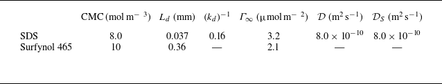


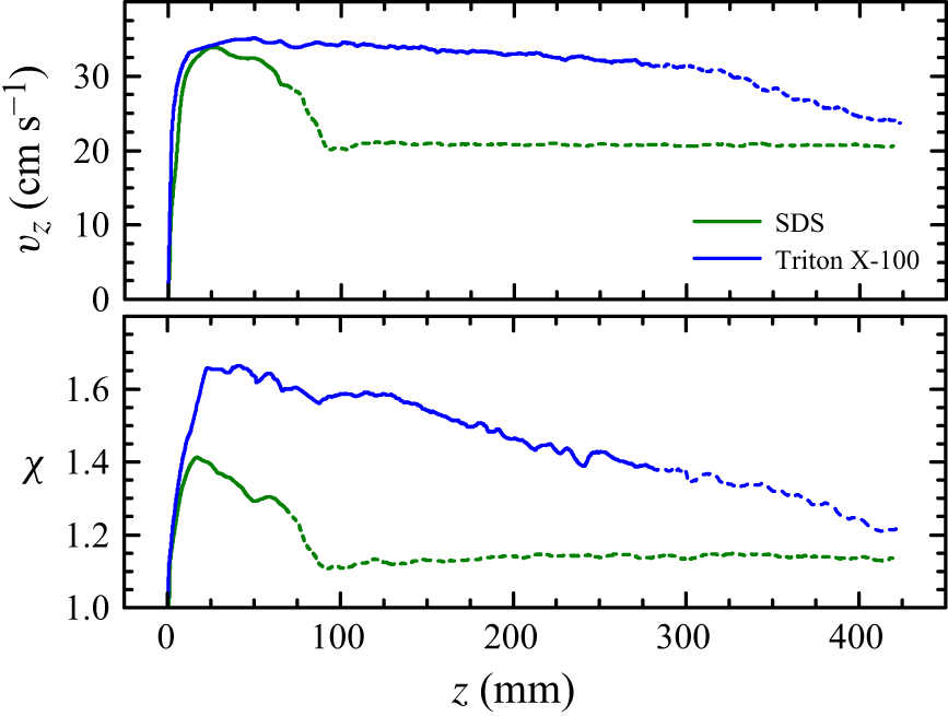


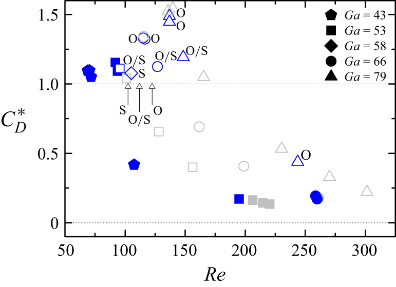

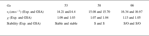


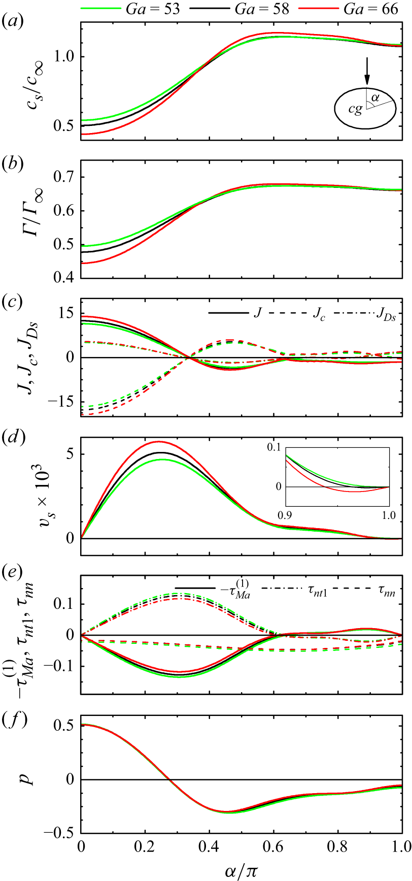


 Open access