





1. Introduction
1.1. Basic principles of stratified flows
The fluid dynamics of a body of size $L$
moving at speed
$L$
moving at speed $U$
through a density gradient
$U$
through a density gradient ${\rm d}\rho /{\rm d}z$
can be described by two dimensionless parameters: the Reynolds number
${\rm d}\rho /{\rm d}z$
can be described by two dimensionless parameters: the Reynolds number $\textit{Re} = UL/\nu$
, and the internal Froude number
$\textit{Re} = UL/\nu$
, and the internal Froude number $\textit{Fr} = U/\textit{NL}$
. The latter can be interpreted as the ratio of the time scale of the restoring buoyancy force,
$\textit{Fr} = U/\textit{NL}$
. The latter can be interpreted as the ratio of the time scale of the restoring buoyancy force, $1/N$
, where
$1/N$
, where $N = \sqrt {-g/\rho _0({\rm d}\rho /{\rm d}z)}$
is the natural frequency of oscillation of fluid particles vertically displaced from their equilibrium position
$N = \sqrt {-g/\rho _0({\rm d}\rho /{\rm d}z)}$
is the natural frequency of oscillation of fluid particles vertically displaced from their equilibrium position $\rho _0$
, to an advective time scale
$\rho _0$
, to an advective time scale $L/U$
. When
$L/U$
. When $\rho (z)$
is such that heavy fluid always lies beneath lighter fluid, the resulting stratification is stable, and a restoring force is exerted on all motions involving departure from that equilibrium. In these flows, wavelike responses with frequencies near
$\rho (z)$
is such that heavy fluid always lies beneath lighter fluid, the resulting stratification is stable, and a restoring force is exerted on all motions involving departure from that equilibrium. In these flows, wavelike responses with frequencies near $N$
are possible. In decaying flows, such as wakes behind moving bodies, the buoyancy forces will eventually dominate, damping out all subsequent vertical motion, and leaving behind quasi-horizontal turbulence that occurs primarily in layers (Lighthill Reference Lighthill1978; Riley, Metcalf & Weissman Reference Riley, Metcalf and Weissman1981; Lilly Reference Lilly1983; Majda & Grote Reference Majda and Grote1997). The wakes of bodies immersed in uniform density gradients have been an enduring object of study (Lin & Pao Reference Lin and Pao1979; Lin et al. Reference Lin, Lindberg, Boyer and Fernando1992; Chomaz et al. Reference Chomaz, Bonetton and Hopfinger1993b
; Spedding et al. Reference Spedding, Browand and Fincham1996b
), partly because even when initial conditions are irregular and turbulent (with high associated values of both
$N$
are possible. In decaying flows, such as wakes behind moving bodies, the buoyancy forces will eventually dominate, damping out all subsequent vertical motion, and leaving behind quasi-horizontal turbulence that occurs primarily in layers (Lighthill Reference Lighthill1978; Riley, Metcalf & Weissman Reference Riley, Metcalf and Weissman1981; Lilly Reference Lilly1983; Majda & Grote Reference Majda and Grote1997). The wakes of bodies immersed in uniform density gradients have been an enduring object of study (Lin & Pao Reference Lin and Pao1979; Lin et al. Reference Lin, Lindberg, Boyer and Fernando1992; Chomaz et al. Reference Chomaz, Bonetton and Hopfinger1993b
; Spedding et al. Reference Spedding, Browand and Fincham1996b
), partly because even when initial conditions are irregular and turbulent (with high associated values of both $\textit{Re}$
and
$\textit{Re}$
and $\textit{Fr}$
), the long-time states can show a notable degree of order and persistence (Spedding Reference Spedding1997, Reference Spedding2014). The emergence of the differing longitudinal and vertical length scales in a strongly stratified flow has been the subject of theoretical interest (Chomaz et al. Reference Chomaz, Bonetton, Butet and Hopfinger1993a
; Riley & Lelong Reference Riley and Lelong2000; Billant & Chomaz Reference Billant and Chomaz2001; Godoy-Diana, Chomaz & Billant Reference Godoy-Diana, Chomaz and Billant2004; Brethouwer et al. Reference Brethouwer, Billant, Lindborg and Chomaz2007; Augier, Galtier & Billant Reference Augier, Galtier and Billant2012; de Bruyn Kops & Riley Reference de Bruyn Kops and Riley2019), with the appearance of novel instability modes (Chomaz et al. Reference Chomaz, Bonetton and Hopfinger1993b
; Godoy-Diana et al. Reference Godoy-Diana, Chomaz and Billant2004; Meunier & Leweke Reference Meunier and Leweke2005; Leweke, Le Dizès & Williamson Reference Leweke, Le Dizès and Williamson2016) unique to stratified ambients.
$\textit{Fr}$
), the long-time states can show a notable degree of order and persistence (Spedding Reference Spedding1997, Reference Spedding2014). The emergence of the differing longitudinal and vertical length scales in a strongly stratified flow has been the subject of theoretical interest (Chomaz et al. Reference Chomaz, Bonetton, Butet and Hopfinger1993a
; Riley & Lelong Reference Riley and Lelong2000; Billant & Chomaz Reference Billant and Chomaz2001; Godoy-Diana, Chomaz & Billant Reference Godoy-Diana, Chomaz and Billant2004; Brethouwer et al. Reference Brethouwer, Billant, Lindborg and Chomaz2007; Augier, Galtier & Billant Reference Augier, Galtier and Billant2012; de Bruyn Kops & Riley Reference de Bruyn Kops and Riley2019), with the appearance of novel instability modes (Chomaz et al. Reference Chomaz, Bonetton and Hopfinger1993b
; Godoy-Diana et al. Reference Godoy-Diana, Chomaz and Billant2004; Meunier & Leweke Reference Meunier and Leweke2005; Leweke, Le Dizès & Williamson Reference Leweke, Le Dizès and Williamson2016) unique to stratified ambients.
As turbulence evolves under significant stratification, the principal local velocity component is in the horizontal, $U_h$
, and together with integral scales in the vertical and horizontal
$U_h$
, and together with integral scales in the vertical and horizontal $(L_v, L_h)$
, may be used to construct local dimensionless numbers
$(L_v, L_h)$
, may be used to construct local dimensionless numbers $\textit{Re}_h = U_hL_h/\nu$
and
$\textit{Re}_h = U_hL_h/\nu$
and $\textit{Fr}_h = U_h/\textit{NL}_h$
. In a drag wake, the dominant local velocity is in the streamwise direction, and this component is used to define
$\textit{Fr}_h = U_h/\textit{NL}_h$
. In a drag wake, the dominant local velocity is in the streamwise direction, and this component is used to define $U_h$
. Several regimes may occur, depending on the balance between inertial, viscous and buoyancy forces. Godoy-Diana et al. (Reference Godoy-Diana, Chomaz and Billant2004) showed that the initial aspect ratio
$U_h$
. Several regimes may occur, depending on the balance between inertial, viscous and buoyancy forces. Godoy-Diana et al. (Reference Godoy-Diana, Chomaz and Billant2004) showed that the initial aspect ratio $\alpha _0 = L_v/L_h$
can also affect the long-time state of a decaying flow. A Reynolds buoyancy number can be written as
$\alpha _0 = L_v/L_h$
can also affect the long-time state of a decaying flow. A Reynolds buoyancy number can be written as $R = \textit{Re}_h\,\textit{Fr}_h^2$
(Brethouwer et al. Reference Brethouwer, Billant, Lindborg and Chomaz2007), and when
$R = \textit{Re}_h\,\textit{Fr}_h^2$
(Brethouwer et al. Reference Brethouwer, Billant, Lindborg and Chomaz2007), and when $R\gg 1$
, the scales larger than the Ozmidov scale
$R\gg 1$
, the scales larger than the Ozmidov scale $l_0$
are strongly influenced by stratification, while the scales between
$l_0$
are strongly influenced by stratification, while the scales between $l_0$
and the Kolmogorov scale
$l_0$
and the Kolmogorov scale $\eta$
are less affected. When
$\eta$
are less affected. When $R\ll 1$
, both viscous diffusion and vertical shearing are important, and the flow arrives at a viscously dominated state, independent of
$R\ll 1$
, both viscous diffusion and vertical shearing are important, and the flow arrives at a viscously dominated state, independent of $N$
(or initial
$N$
(or initial $\textit{Fr}$
). Authors de Bruyn Kops & Riley (Reference de Bruyn Kops and Riley2019) introduced an activity parameter
$\textit{Fr}$
). Authors de Bruyn Kops & Riley (Reference de Bruyn Kops and Riley2019) introduced an activity parameter $G = \textit{Re}_t\,\textit{Fr}_t^2$
that is similar to
$G = \textit{Re}_t\,\textit{Fr}_t^2$
that is similar to $R$
, but based on total turbulent length and velocity scales, which marks the scale range between
$R$
, but based on total turbulent length and velocity scales, which marks the scale range between $l_0$
and
$l_0$
and $\eta$
. Note that
$\eta$
. Note that $R$
and
$R$
and $G$
are not equivalent as the different velocity and length scales evolve differently. As a given stratified flow decays through a trajectory in
$G$
are not equivalent as the different velocity and length scales evolve differently. As a given stratified flow decays through a trajectory in $G{-}\textit{Fr}_h$
space, the initial three-dimensional buoyancy controlled and viscous controlled regimes mapped out for stratified wakes (Spedding Reference Spedding1997) are retraced, hereafter abbreviated as 3D-NEQ-Q2D. As
$G{-}\textit{Fr}_h$
space, the initial three-dimensional buoyancy controlled and viscous controlled regimes mapped out for stratified wakes (Spedding Reference Spedding1997) are retraced, hereafter abbreviated as 3D-NEQ-Q2D. As $G$
decreases from an initially high value to order 1, the dynamics of shearing between decoupled layers becomes important, as shown by Diamessis, Spedding & Domaradzki (Reference Diamessis, Spedding and Domaradzki2011) and de Bruyn Kops & Riley (Reference de Bruyn Kops and Riley2019), where secondary production of turbulence through Kelvin–Helmholtz instability is responsible for prolonging the energetic turbulence. The breadth of the scale range allowing for turbulent motion, relatively unaffected by buoyancy or viscosity (as measured by
$G$
decreases from an initially high value to order 1, the dynamics of shearing between decoupled layers becomes important, as shown by Diamessis, Spedding & Domaradzki (Reference Diamessis, Spedding and Domaradzki2011) and de Bruyn Kops & Riley (Reference de Bruyn Kops and Riley2019), where secondary production of turbulence through Kelvin–Helmholtz instability is responsible for prolonging the energetic turbulence. The breadth of the scale range allowing for turbulent motion, relatively unaffected by buoyancy or viscosity (as measured by $G$
), leads to varying amounts of time when the turbulence can sustain and where secondary turbulence can be generated.
$G$
), leads to varying amounts of time when the turbulence can sustain and where secondary turbulence can be generated.
The topic is not only of abstract importance, as most flight and underwater vehicles spend much of their time travelling horizontally through a stable density gradient. In both cases, the persistence of quasi-horizontal motions and the remarkably compact nature of the late wake is a practical matter for the wake creator and potential wake detector. In MKS units, an aircraft has $U = \mathcal{O}(10^2)$
, with
$U = \mathcal{O}(10^2)$
, with $L = \mathcal{O}(10)$
, and a submarine has
$L = \mathcal{O}(10)$
, and a submarine has $U = \mathcal{O}(10)$
and
$U = \mathcal{O}(10)$
and $L = \mathcal{O}(10)$
. We have
$L = \mathcal{O}(10)$
. We have $N = \mathcal{O}(10^{-2})$
and
$N = \mathcal{O}(10^{-2})$
and $\mathcal{O}(10^{-3})$
rad s−1 in the troposphere and the ocean thermocline, respectively, so
$\mathcal{O}(10^{-3})$
rad s−1 in the troposphere and the ocean thermocline, respectively, so $\textit{Fr}$
in both air and seawater is
$\textit{Fr}$
in both air and seawater is $\mathcal{O}(10^3)$
, while
$\mathcal{O}(10^3)$
, while $\textit{Re} = \mathcal{O}(10^8)$
. Energy is distributed over a broad range of scales, and many eddy turnover times elapse before one buoyancy period. The high
$\textit{Re} = \mathcal{O}(10^8)$
. Energy is distributed over a broad range of scales, and many eddy turnover times elapse before one buoyancy period. The high $\textit{Re}$
regime presents challenges for laboratory experiment and numerical simulation, and while
$\textit{Re}$
regime presents challenges for laboratory experiment and numerical simulation, and while $\textit{Fr}$
of the order of
$\textit{Fr}$
of the order of $10^2$
has been realised in experiment, there is also some evidence that
$10^2$
has been realised in experiment, there is also some evidence that $\textit{Fr}$
independence is seen for
$\textit{Fr}$
independence is seen for $\textit{Fr} \geqslant 10$
(Spedding Reference Spedding1997). Given these considerations, some effort has gone into exploring how relationships may scale with
$\textit{Fr} \geqslant 10$
(Spedding Reference Spedding1997). Given these considerations, some effort has gone into exploring how relationships may scale with $\textit{Re}$
and
$\textit{Re}$
and $\textit{Fr}$
, in addition to a focus on body geometries that more closely resemble practical applications.
$\textit{Fr}$
, in addition to a focus on body geometries that more closely resemble practical applications.
1.2. The axisymmetric stratified drag wake
The flow around a sphere has been studied in experiments and dye visualisations (e.g. Lin et al. Reference Lin, Lindberg, Boyer and Fernando1992; Chomaz et al. Reference Chomaz, Bonetton and Hopfinger1993b
; Chashechkin Reference Chashechkin2022), which show intricate and beautiful near-wake patterns and deduced lines of separation on the body. Values of $\textit{Re}$
and
$\textit{Re}$
and $\textit{Fr}$
were varied in mostly low-Re, low-
$\textit{Fr}$
were varied in mostly low-Re, low- $\textit{Fr}$
regimes, so the strong influence of boundary layer separation with strong buoyancy constraints results in multiple topological patterns and models. As
$\textit{Fr}$
regimes, so the strong influence of boundary layer separation with strong buoyancy constraints results in multiple topological patterns and models. As $\textit{Re}$
and
$\textit{Re}$
and $\textit{Fr}$
are increased, Chomaz et al. (Reference Chomaz, Bonetton and Hopfinger1993b) noted that for
$\textit{Fr}$
are increased, Chomaz et al. (Reference Chomaz, Bonetton and Hopfinger1993b) noted that for $\textit{Fr}\geqslant4.5$
, fully three-dimensional modes appeared in the near wake, and a criterion for
$\textit{Fr}\geqslant4.5$
, fully three-dimensional modes appeared in the near wake, and a criterion for $\textit{Fr}\geqslant3$
was outlined by Spedding et al. (Reference Spedding, Browand and Fincham1996a) for an integral scale of turbulence to lie beneath the limiting Ozmidov scale imposed by buoyancy. Spedding et al. (Reference Spedding, Browand and Fincham1996b) demonstrated empirical collapse of late wakes onto general scaling laws for initially turbulent conditions, provided that
$\textit{Fr}\geqslant3$
was outlined by Spedding et al. (Reference Spedding, Browand and Fincham1996a) for an integral scale of turbulence to lie beneath the limiting Ozmidov scale imposed by buoyancy. Spedding et al. (Reference Spedding, Browand and Fincham1996b) demonstrated empirical collapse of late wakes onto general scaling laws for initially turbulent conditions, provided that $\textit{Fr}\geqslant4$
and
$\textit{Fr}\geqslant4$
and $\textit{Re}\geqslant 5000$
. The observed scaling relations do not depend on body geometry (Meunier & Spedding Reference Meunier and Spedding2004), and disturbance amplitudes could be rescaled based on known drag coefficients, which reflect the horizontal mass flux for the unstratified condition. The implications are at once normal and surprising. The normal expectation for axisymmetric turbulent wakes (Tennekes & Lumley Reference Tennekes and Lumley1972; Townsend Reference Townsend1976) is self-similar evolution of turbulence that feels only local dynamical constraints, while the surprising aspect is that such approximations continue to work even at late times in a stratified system, when the flow is far from turbulent, or isotropic. Contradictions remain: experiments in unstratified conditions have shown long-lasting influence of initial conditions (Bevilaqua & Lykoudis Reference Bevilaqua and Lykoudis1978; George Reference George1989), and Nedić et al. (Reference Nedić, Vassilicos and Ganapathisubramani2013) showed how allowing for non-equilibrium conditions can lead to different scaling relations, specifically to
$\textit{Re}\geqslant 5000$
. The observed scaling relations do not depend on body geometry (Meunier & Spedding Reference Meunier and Spedding2004), and disturbance amplitudes could be rescaled based on known drag coefficients, which reflect the horizontal mass flux for the unstratified condition. The implications are at once normal and surprising. The normal expectation for axisymmetric turbulent wakes (Tennekes & Lumley Reference Tennekes and Lumley1972; Townsend Reference Townsend1976) is self-similar evolution of turbulence that feels only local dynamical constraints, while the surprising aspect is that such approximations continue to work even at late times in a stratified system, when the flow is far from turbulent, or isotropic. Contradictions remain: experiments in unstratified conditions have shown long-lasting influence of initial conditions (Bevilaqua & Lykoudis Reference Bevilaqua and Lykoudis1978; George Reference George1989), and Nedić et al. (Reference Nedić, Vassilicos and Ganapathisubramani2013) showed how allowing for non-equilibrium conditions can lead to different scaling relations, specifically to $U_0 \sim x^{-1}$
and
$U_0 \sim x^{-1}$
and $L_h \sim x^{1/2}$
, and close agreement has been found in experiment on spheres at varying
$L_h \sim x^{1/2}$
, and close agreement has been found in experiment on spheres at varying $\textit{Re}$
and
$\textit{Re}$
and $C_D$
by Saunders et al. (Reference Saunders, Frederick, Drivas and Wunsch2020, Reference Saunders, Britt and Wunsch2022). In numerical simulations of stratified wakes, Redford, Castro & Coleman (Reference Redford, Castro and Coleman2012) demonstrated the continuing influence of initial conditions far downstream. In numerical and physical experiments, the power-law exponents sometimes match classical examples, where wake width and defect velocity scale as
$C_D$
by Saunders et al. (Reference Saunders, Frederick, Drivas and Wunsch2020, Reference Saunders, Britt and Wunsch2022). In numerical simulations of stratified wakes, Redford, Castro & Coleman (Reference Redford, Castro and Coleman2012) demonstrated the continuing influence of initial conditions far downstream. In numerical and physical experiments, the power-law exponents sometimes match classical examples, where wake width and defect velocity scale as $L_h \sim x^{1/3}$
and
$L_h \sim x^{1/3}$
and $U_0 \sim x^{-2/3}$
(Jimenez, Hultmark & Smits Reference Jimenez, Hultmark and Smits2010; Kumar & Mahesh Reference Kumar and Mahesh2018; Ortiz-Tarin, Nidhan & Sarkar Reference Ortiz-Tarin, Nidhan and Sarkar2021), and sometimes do not (Bonnier & Eiff Reference Bonnier and Eiff2002; Pal et al. Reference Pal, Sarkar, Posa and Balaras2017; Ortiz-Tarin, Chongsiripinyo & Sarkar Reference Ortiz-Tarin, Chongsiripinyo and Sarkar2019), and it remains unclear when equilibrium conditions can be presumed. The most recent and detailed measurements and computations on flat-plate disk models (Dairay, Obligado & Vassilicos Reference Dairay, Obligado and Vassilicos2015) suggest that
$U_0 \sim x^{-2/3}$
(Jimenez, Hultmark & Smits Reference Jimenez, Hultmark and Smits2010; Kumar & Mahesh Reference Kumar and Mahesh2018; Ortiz-Tarin, Nidhan & Sarkar Reference Ortiz-Tarin, Nidhan and Sarkar2021), and sometimes do not (Bonnier & Eiff Reference Bonnier and Eiff2002; Pal et al. Reference Pal, Sarkar, Posa and Balaras2017; Ortiz-Tarin, Chongsiripinyo & Sarkar Reference Ortiz-Tarin, Chongsiripinyo and Sarkar2019), and it remains unclear when equilibrium conditions can be presumed. The most recent and detailed measurements and computations on flat-plate disk models (Dairay, Obligado & Vassilicos Reference Dairay, Obligado and Vassilicos2015) suggest that $U_0 \sim x^{-1}$
and
$U_0 \sim x^{-1}$
and $L_h \sim x^{1/2}$
may be quite general. Li, Yang & Kunz (Reference Li, Yang and Kunz2024) conducted multiple simulations to show that in some cases, uncertainty in establishing power-law coefficients comes from the small number of experimental or computational realisations of any given condition. Moreover, certain of these disagreements arise when near- and far-wake quantities are compared, as scale similarity is not expected until
$L_h \sim x^{1/2}$
may be quite general. Li, Yang & Kunz (Reference Li, Yang and Kunz2024) conducted multiple simulations to show that in some cases, uncertainty in establishing power-law coefficients comes from the small number of experimental or computational realisations of any given condition. Moreover, certain of these disagreements arise when near- and far-wake quantities are compared, as scale similarity is not expected until $x/D\geqslant50$
, and different quantities may converge at different downstream distances that may be very large (George Reference George1989).
$x/D\geqslant50$
, and different quantities may converge at different downstream distances that may be very large (George Reference George1989).
The comparative unimportance of the body geometry observed by Meunier & Spedding (Reference Meunier and Spedding2004) encouraged early temporal simulations where the initial conditions comprised a mean defect with embedded turbulence (Gourlay et al. Reference Gourlay, Arendt, Fritts and Werne2001; Dommermuth et al. Reference Dommermuth, Rottman, Innis and Novikov2002; Diamessis et al. Reference Diamessis, Spedding and Domaradzki2011), and both experiment and simulation have expanded their reach into self-propelled bodies (Meunier & Spedding Reference Meunier and Spedding2006; Brucker & Sarkar Reference Brucker and Sarkar2010), the operationally inspired source of much of the early experimental work (Lin & Pao Reference Lin and Pao1979). Temporal simulations begin with a slab, or tube, of turbulence on a mean profile, and investigate the dynamics as stratification is imposed gradually and then evolves in time. In this way, it is possible to push the Reynolds numbers to $\mathcal{O}(10^6)$
, which, though still two orders of magnitude below field conditions, does allow for the large turbulent scale range (
$\mathcal{O}(10^6)$
, which, though still two orders of magnitude below field conditions, does allow for the large turbulent scale range ( $G \gg 1,\ R \gg 1$
) and development of secondary turbulence, as discussed by Zhou & Diamessis (Reference Zhou and Diamessis2019) and de Bruyn Kops & Riley (Reference de Bruyn Kops and Riley2019).
$G \gg 1,\ R \gg 1$
) and development of secondary turbulence, as discussed by Zhou & Diamessis (Reference Zhou and Diamessis2019) and de Bruyn Kops & Riley (Reference de Bruyn Kops and Riley2019).
1.3. The influence of body geometry
It is only when initial $\textit{Re}$
and
$\textit{Re}$
and $\textit{Fr}$
have some minimum value that one might expect self-similar turbulence to emerge over a sufficient range of scales (akin to a requirement for
$\textit{Fr}$
have some minimum value that one might expect self-similar turbulence to emerge over a sufficient range of scales (akin to a requirement for $G \gg 1,\ R \gg 1$
). Otherwise, it has been demonstrated for disk wakes (Xiang et al. Reference Xiang, Madison, Sellappan and Spedding2015) and sphere wakes (Madison, Xiang & Spedding Reference Madison, Xiang and Spedding2022) that no body-independent (or initial-condition-independent) signature occurs in in the near wake (
$G \gg 1,\ R \gg 1$
). Otherwise, it has been demonstrated for disk wakes (Xiang et al. Reference Xiang, Madison, Sellappan and Spedding2015) and sphere wakes (Madison, Xiang & Spedding Reference Madison, Xiang and Spedding2022) that no body-independent (or initial-condition-independent) signature occurs in in the near wake ( $x/D \leqslant 15$
,
$x/D \leqslant 15$
, $\textit{Nt} \leqslant 20$
) for
$\textit{Nt} \leqslant 20$
) for $\textit{Re} \leqslant 10^4$
,
$\textit{Re} \leqslant 10^4$
, $\textit{Fr} \leqslant9$
. The first simulations that included a body in a stratified background were at moderately low
$\textit{Fr} \leqslant9$
. The first simulations that included a body in a stratified background were at moderately low $\textit{Re}\leqslant 5000$
,
$\textit{Re}\leqslant 5000$
, $\textit{Fr} \leqslant4$
(Hanazaki Reference Hanazaki1988; Orr et al. Reference Orr, Domaradzki, Spedding and Constantinescu2015; Pal et al. Reference Pal, Sarkar, Posa and Balaras2016, Reference Pal, Sarkar, Posa and Balaras2017) when no broad range of scales enabling turbulence could be expected. As reachable
$\textit{Fr} \leqslant4$
(Hanazaki Reference Hanazaki1988; Orr et al. Reference Orr, Domaradzki, Spedding and Constantinescu2015; Pal et al. Reference Pal, Sarkar, Posa and Balaras2016, Reference Pal, Sarkar, Posa and Balaras2017) when no broad range of scales enabling turbulence could be expected. As reachable $\textit{Re}$
for simulations steadily increases, attention has also turned to slender bodies and their near- and far-wakes; Ortiz-Tarin et al. (Reference Ortiz-Tarin, Chongsiripinyo and Sarkar2019) showed a geometry dependence in the near wake, while far-wake statistics appeared similar to those established for spheres and slender bodies (Meunier & Spedding Reference Meunier and Spedding2004). Though
$\textit{Re}$
for simulations steadily increases, attention has also turned to slender bodies and their near- and far-wakes; Ortiz-Tarin et al. (Reference Ortiz-Tarin, Chongsiripinyo and Sarkar2019) showed a geometry dependence in the near wake, while far-wake statistics appeared similar to those established for spheres and slender bodies (Meunier & Spedding Reference Meunier and Spedding2004). Though $\textit{Re} = 10^4$
was high enough to permit turbulence, the highest value of
$\textit{Re} = 10^4$
was high enough to permit turbulence, the highest value of $\textit{Fr}=3$
makes it unlikely that an initial, buoyancy-independent stage could exist. The development of hybrid simulations allowed moderately high
$\textit{Fr}=3$
makes it unlikely that an initial, buoyancy-independent stage could exist. The development of hybrid simulations allowed moderately high $\textit{Re}$
cases to be run for longer times/downstream distances, and an unstratified simulation of a 6 : 1 spheroid at
$\textit{Re}$
cases to be run for longer times/downstream distances, and an unstratified simulation of a 6 : 1 spheroid at $\textit{Re} = 10^5$
by Ortiz-Tarin et al. Reference Ortiz-Tarin, Nidhan and Sarkar2021 showed that although near-wake statistics were consistent with the classical
$\textit{Re} = 10^5$
by Ortiz-Tarin et al. Reference Ortiz-Tarin, Nidhan and Sarkar2021 showed that although near-wake statistics were consistent with the classical $-2/3$
decay of the defect velocity, between
$-2/3$
decay of the defect velocity, between $x/D = 20$
and
$x/D = 20$
and $x/D = 80$
, a decay law closer to
$x/D = 80$
, a decay law closer to $-6/5$
was established, and only then could self-similarity be claimed. Figure 1 in that paper vividly demonstrates the variation in the literature on bluff and slender bodies in an unstratified medium. When the hybrid simulations were deployed for stratified wakes of a 6 : 1 slender body and a disk (Ortiz-Tarin, Nidhan & Sarkar Reference Ortiz-Tarin, Nidhan and Sarkar2023), the characteristic transition points marking 3D-NEQ-Q2D varied according to the body shape (we may note that no universal transition point in
$-6/5$
was established, and only then could self-similarity be claimed. Figure 1 in that paper vividly demonstrates the variation in the literature on bluff and slender bodies in an unstratified medium. When the hybrid simulations were deployed for stratified wakes of a 6 : 1 slender body and a disk (Ortiz-Tarin, Nidhan & Sarkar Reference Ortiz-Tarin, Nidhan and Sarkar2023), the characteristic transition points marking 3D-NEQ-Q2D varied according to the body shape (we may note that no universal transition point in $\textit{Nt}$
has been claimed for the NEQ-Q2D point), and no universal scaling was uncovered for
$\textit{Nt}$
has been claimed for the NEQ-Q2D point), and no universal scaling was uncovered for $\textit{Re} = 10^5$
, and a maximum
$\textit{Re} = 10^5$
, and a maximum $\textit{Fr}=10$
. It was acknowledged that the parameters of the simulation did not allow the slender body case to access the strongly stratified turbulence regime in
$\textit{Fr}=10$
. It was acknowledged that the parameters of the simulation did not allow the slender body case to access the strongly stratified turbulence regime in $G{-}\textit{Fr}_h$
space. The obvious advantage of finding reasonable approximations to scaling laws that can derive from simple model formulations (Tennekes & Lumley Reference Tennekes and Lumley1972; Townsend Reference Townsend1976; Meunier, Diamessis & Spedding Reference Meunier, Diamessis and Spedding2006) is that extrapolations over
$G{-}\textit{Fr}_h$
space. The obvious advantage of finding reasonable approximations to scaling laws that can derive from simple model formulations (Tennekes & Lumley Reference Tennekes and Lumley1972; Townsend Reference Townsend1976; Meunier, Diamessis & Spedding Reference Meunier, Diamessis and Spedding2006) is that extrapolations over $\textit{Re}$
and
$\textit{Re}$
and $\textit{Fr}$
can be predicted, and then tested. Absent some theoretical backing, the search for empirical power-law approximations is not necessarily informative, particularly if there is doubt over the original self-similar dynamics. The simplifications of laboratory and numerical simulations (steady
$\textit{Fr}$
can be predicted, and then tested. Absent some theoretical backing, the search for empirical power-law approximations is not necessarily informative, particularly if there is doubt over the original self-similar dynamics. The simplifications of laboratory and numerical simulations (steady $U$
motion, parallel to a pycnocline in a linear density gradient that extends far from the body) may preclude the investigation of departures from this ideal that are nonetheless of operational importance. For example, Meunier & Spedding (Reference Meunier and Spedding2006) showed that exactly self-propelled wakes were identifiably different from all other jets or wakes, but that an imagined 30 m length slender, self-propelled body would only reach equilibrium after 1 km following a small change in propulsion. In that study, a small change in incidence angle of the slender body had a strong influence close to the self-propelled point, and Gallet, Meunier & Spedding (Reference Gallet, Meunier and Spedding2006) found that wake asymmetry caused by small yaw angles persisted into the late wake regime at
$U$
motion, parallel to a pycnocline in a linear density gradient that extends far from the body) may preclude the investigation of departures from this ideal that are nonetheless of operational importance. For example, Meunier & Spedding (Reference Meunier and Spedding2006) showed that exactly self-propelled wakes were identifiably different from all other jets or wakes, but that an imagined 30 m length slender, self-propelled body would only reach equilibrium after 1 km following a small change in propulsion. In that study, a small change in incidence angle of the slender body had a strong influence close to the self-propelled point, and Gallet, Meunier & Spedding (Reference Gallet, Meunier and Spedding2006) found that wake asymmetry caused by small yaw angles persisted into the late wake regime at $\textit{Nt} = 100$
.
$\textit{Nt} = 100$
.
Schematic of the experimental set-up and field of view (FOV), with labelled coordinate system.

The question of breaking the symmetry of the wake generator is clearly relevant, and recent work, prompted by practical application, has used an inclined spheroid as such an example. The location and geometry of separation lines can be complex, varying with inclination angle $\theta$
, and
$\theta$
, and $\textit{Re}$
. In a strongly stratified flow at low
$\textit{Re}$
. In a strongly stratified flow at low $\textit{Fr}$
, buoyancy forces will also change the near-surface flow, especially for a natural wavelength
$\textit{Fr}$
, buoyancy forces will also change the near-surface flow, especially for a natural wavelength $\lambda /D = \pi\, \textit{Fr}_L$
, where
$\lambda /D = \pi\, \textit{Fr}_L$
, where $\textit{Fr}_L$
is a Froude number based on half body length. The stratified flow around and behind an inclined spheroid has been studied by experiment (Ohh & Spedding Reference Ohh and Spedding2024) (hereafter denoted OS24) and simulation (Nidhan et al. Reference Nidhan, Jain, Ortiz-Tarin and Sarkar2025). When
$\textit{Fr}_L$
is a Froude number based on half body length. The stratified flow around and behind an inclined spheroid has been studied by experiment (Ohh & Spedding Reference Ohh and Spedding2024) (hereafter denoted OS24) and simulation (Nidhan et al. Reference Nidhan, Jain, Ortiz-Tarin and Sarkar2025). When $\textit{Fr}_L = 2U/\textit{NL} = 1$
, maximum resonance of an internal half-wavelength over the length of the body occurs, so it is a convenient and physically relevant measure; at the same time, we retain
$\textit{Fr}_L = 2U/\textit{NL} = 1$
, maximum resonance of an internal half-wavelength over the length of the body occurs, so it is a convenient and physically relevant measure; at the same time, we retain $\textit{Re}_D$
for a Reynolds number based on diameter. Nidhan et al. (Reference Nidhan, Jain, Ortiz-Tarin and Sarkar2025) conducted large-eddy simulations at
$\textit{Re}_D$
for a Reynolds number based on diameter. Nidhan et al. (Reference Nidhan, Jain, Ortiz-Tarin and Sarkar2025) conducted large-eddy simulations at $\textit{Re}_D = 5 \times 10^3$
,
$\textit{Re}_D = 5 \times 10^3$
, $\textit{Fr}_L = \infty , 1, 1/3, 1/6$
and
$\textit{Fr}_L = \infty , 1, 1/3, 1/6$
and $\theta = 10^\circ$
, with
$\theta = 10^\circ$
, with $x/D$
up to 40. OS24 explored a range of
$x/D$
up to 40. OS24 explored a range of $\textit{Re}_D$
from
$\textit{Re}_D$
from $5\times10^3$
to
$5\times10^3$
to $20\times 10^3$
,
$20\times 10^3$
, $\textit{Fr}_L = 2.6, 5.2, 10.4$
and
$\textit{Fr}_L = 2.6, 5.2, 10.4$
and $\theta = 0^\circ, 10^\circ, 20^\circ$
, covering
$\theta = 0^\circ, 10^\circ, 20^\circ$
, covering $x/D$
up to
$x/D$
up to $10^2$
, and
$10^2$
, and $\textit{Nt} \approx 10^1$
. The stratified cases of Nidhan et al. (Reference Nidhan, Jain, Ortiz-Tarin and Sarkar2025) must be considered strongly stratified, while the experiments in OS24 extend into the more weakly constrained case. At the higher
$\textit{Nt} \approx 10^1$
. The stratified cases of Nidhan et al. (Reference Nidhan, Jain, Ortiz-Tarin and Sarkar2025) must be considered strongly stratified, while the experiments in OS24 extend into the more weakly constrained case. At the higher $\textit{Fr}$
and
$\textit{Fr}$
and $\theta$
, both studies describe the existence of separation vortices that coexist with the more narrow drag wake, and persist downstream, though later wake measurements showed a merging of the defect profiles that grow in height and decay in strength much as the axisymmetric
$\theta$
, both studies describe the existence of separation vortices that coexist with the more narrow drag wake, and persist downstream, though later wake measurements showed a merging of the defect profiles that grow in height and decay in strength much as the axisymmetric $\theta = 0^\circ$
case does. Evidence was given for continued asymmetry of the streamwise vortices, and for a large-scale undulation with period
$\theta = 0^\circ$
case does. Evidence was given for continued asymmetry of the streamwise vortices, and for a large-scale undulation with period $2\pi /N$
excited by the large-scale separation vortices at non-zero
$2\pi /N$
excited by the large-scale separation vortices at non-zero $\theta$
.
$\theta$
.
1.4. Objectives
While OS24 covered a range of $(\textit{Re},\textit{Fr})$
, these parameters were varied together by changing
$(\textit{Re},\textit{Fr})$
, these parameters were varied together by changing $U$
for a fixed
$U$
for a fixed $N$
, so the effects of Reynolds number and Froude number could not be fully isolated. The present work describes the outcomes of an independent variation of
$N$
, so the effects of Reynolds number and Froude number could not be fully isolated. The present work describes the outcomes of an independent variation of $\textit{Re}$
and
$\textit{Re}$
and $\textit{Fr}$
, allowing the influences of inertia and stratification to be examined separately. In addition, an effort was made to collect reliable statistics through multiple runs at each parameter pair. In evaluating the stratified cases with respect to an unstratified baseline, it was necessary to compile extensive unstratified wake data that do not yet exist in a complete database. The time-averaged statistical measurements are then related to the instantaneous wake structure, and the proposed instabilities identified in OS24 are examined. Finally, we revisit far-wake scaling laws with the goal of identifying which characteristics show the imprint of a non-axisymmetric wake generator.
$\textit{Fr}$
, allowing the influences of inertia and stratification to be examined separately. In addition, an effort was made to collect reliable statistics through multiple runs at each parameter pair. In evaluating the stratified cases with respect to an unstratified baseline, it was necessary to compile extensive unstratified wake data that do not yet exist in a complete database. The time-averaged statistical measurements are then related to the instantaneous wake structure, and the proposed instabilities identified in OS24 are examined. Finally, we revisit far-wake scaling laws with the goal of identifying which characteristics show the imprint of a non-axisymmetric wake generator.
2. Materials and methods
2.1. Tank
Experiments were conducted in a 1 m $\times$
1 m
$\times$
1 m $\times$
2.5 m tow tank (figure 1). For stratified experiments, a linear, stable stratification was generated using the standard two-tank method, with ethanol added to avoid optical distortion, following the refractive index matching technique of Xiang et al. (Reference Xiang, Madison, Sellappan and Spedding2015). Salt served as the stratifying agent. The density profile was measured by extracting fluid samples at discrete depths, and measuring their density using a Mettler Toledo PortableLab refractometer. Density profiles were measured for each tank fill, both prior to any experiments and after all experiments were completed, and remained within 5
$\times$
2.5 m tow tank (figure 1). For stratified experiments, a linear, stable stratification was generated using the standard two-tank method, with ethanol added to avoid optical distortion, following the refractive index matching technique of Xiang et al. (Reference Xiang, Madison, Sellappan and Spedding2015). Salt served as the stratifying agent. The density profile was measured by extracting fluid samples at discrete depths, and measuring their density using a Mettler Toledo PortableLab refractometer. Density profiles were measured for each tank fill, both prior to any experiments and after all experiments were completed, and remained within 5 $\,\%$
of targeted
$\,\%$
of targeted ${\rm d}\rho /{\rm d}z$
. The working temperature was maintained at
${\rm d}\rho /{\rm d}z$
. The working temperature was maintained at $21\,^\circ\text{C}$
. Because
$21\,^\circ\text{C}$
. Because $\rho$
and
$\rho$
and $\mu$
vary with depth due to salt and ethanol gradients, the Reynolds number slightly varies along the vertical extent of the body. The Reynolds number calculated using local fluid properties at
$\mu$
vary with depth due to salt and ethanol gradients, the Reynolds number slightly varies along the vertical extent of the body. The Reynolds number calculated using local fluid properties at $z/D = \pm 1$
remained within 1.6
$z/D = \pm 1$
remained within 1.6 $\,\%$
of the target Reynolds number.
$\,\%$
of the target Reynolds number.
2.2. Body and suspension
Spheroids with a 6 : 1 aspect ratio were towed horizontally through a tank filled with stratified salt solution at inclination angles $\theta = 0^\circ$
and
$\theta = 0^\circ$
and $20^\circ$
, following the methods of OS24, except that the body was mounted to the motor-controlled linear traverse via four rigid struts rather than suspended by flexible wires. The spheroid was three-dimensionally printed and permanently mounted to struts of diameter
$20^\circ$
, following the methods of OS24, except that the body was mounted to the motor-controlled linear traverse via four rigid struts rather than suspended by flexible wires. The spheroid was three-dimensionally printed and permanently mounted to struts of diameter $d/D = 0.045$
(figure 2), which were in turn fixed to a carriage towed by a DC stepper motor. Two inclination angles were tested, requiring separate spheroid–strut assemblies for each case. The struts held the spheroid at a fixed
$d/D = 0.045$
(figure 2), which were in turn fixed to a carriage towed by a DC stepper motor. Two inclination angles were tested, requiring separate spheroid–strut assemblies for each case. The struts held the spheroid at a fixed $\theta$
throughout the tow, with pitch angle variation remaining below 1
$\theta$
throughout the tow, with pitch angle variation remaining below 1 $^\circ$
across the field of view, even when subject to significant body forces resulting from high tow speeds (figure 3). Yaw uncertainty, estimated from reconstructed flow fields, was approximately 1
$^\circ$
across the field of view, even when subject to significant body forces resulting from high tow speeds (figure 3). Yaw uncertainty, estimated from reconstructed flow fields, was approximately 1 $^\circ$
. The struts did not intersect the measurement plane and therefore did not contaminate the near wake.
$^\circ$
. The struts did not intersect the measurement plane and therefore did not contaminate the near wake.
A trip wire was printed directly onto the spheroid at $x/L = 0.2$
. The trip had thickness
$x/L = 0.2$
. The trip had thickness $k/\delta = 0.2$
, where
$k/\delta = 0.2$
, where $\delta$
is the estimated boundary layer thickness based on flat-plate assumptions, following the approach of OS24.
$\delta$
is the estimated boundary layer thickness based on flat-plate assumptions, following the approach of OS24.
Front and side views of the spheroid model and suspension wires for 0 $^\circ$
inclination angle (a) and 20
$^\circ$
inclination angle (a) and 20 $^\circ$
inclination angle (b).
$^\circ$
inclination angle (b).

Measured spheroid inclination angle with downstream distance, with the experimental field of view shown in green.

2.3. Ranges of $(\textit{Re},\textit{Fr})$

The tow speed $U$
varied between 0.03 and 0.5 m s−1, and the stratification strength
$U$
varied between 0.03 and 0.5 m s−1, and the stratification strength $N$
was chosen to target specific Froude numbers
$N$
was chosen to target specific Froude numbers $\textit{Fr}_D$
. The resulting parameter space spans Reynolds numbers
$\textit{Fr}_D$
. The resulting parameter space spans Reynolds numbers $\textit{Re}_D = [1.25, 2.5, 5, 10, 20] \times 10^3$
and Froude numbers
$\textit{Re}_D = [1.25, 2.5, 5, 10, 20] \times 10^3$
and Froude numbers $\textit{Fr}_D = [2, 4, 8, 16, 32, \infty ]$
, with
$\textit{Fr}_D = [2, 4, 8, 16, 32, \infty ]$
, with $\textit{Fr}_D = \infty$
corresponding to unstratified conditions. (Henceforth we will assume
$\textit{Fr}_D = \infty$
corresponding to unstratified conditions. (Henceforth we will assume $\textit{Re}$
and
$\textit{Re}$
and $\textit{Fr}$
based on body diameter
$\textit{Fr}$
based on body diameter $D$
, unless noted otherwise.) Experiments at constant
$D$
, unless noted otherwise.) Experiments at constant $N$
are shown by diagonal lines in figure 4. In figure 5 and subsequent figures, each case is labelled RxxFyy
$N$
are shown by diagonal lines in figure 4. In figure 5 and subsequent figures, each case is labelled RxxFyy $\theta$
zz for
$\theta$
zz for $\textit{Re}=\text{xx}\times 10^3$
,
$\textit{Re}=\text{xx}\times 10^3$
, $\textit{Fr} = \text{yy}$
and inclination angle zz degrees. For example, a case at
$\textit{Fr} = \text{yy}$
and inclination angle zz degrees. For example, a case at $\textit{Re} = 5000$
,
$\textit{Re} = 5000$
, $\textit{Fr} = 16$
and
$\textit{Fr} = 16$
and $\theta = 20^\circ$
is denoted R5F16
$\theta = 20^\circ$
is denoted R5F16 $\theta$
20.
$\theta$
20.
The Fr– $\textit{Re}$
parameter space of experiments.
$\textit{Re}$
parameter space of experiments.

2.4. Field of view and domain of boundary-free observation
The tank was filled to depth $18D$
. The spheroid was towed over streamwise distance
$18D$
. The spheroid was towed over streamwise distance $50D$
, entering the measurement region at
$50D$
, entering the measurement region at $18D$
, and exiting at
$18D$
, and exiting at $32D$
, sufficiently far from the start and stop positions to avoid (at least initially) contamination by transient effects. Internal wave reflections from the tank boundaries were considered when determining the usable observation window. The maximum group velocity of internal waves produced by the body is
$32D$
, sufficiently far from the start and stop positions to avoid (at least initially) contamination by transient effects. Internal wave reflections from the tank boundaries were considered when determining the usable observation window. The maximum group velocity of internal waves produced by the body is $\textit{ND}/\pi$
, so sidewall reflections could return after
$\textit{ND}/\pi$
, so sidewall reflections could return after $\textit{Nt} \approx 25\pi$
, which corresponds to
$\textit{Nt} \approx 25\pi$
, which corresponds to $x/D \geqslant 150$
(depending on
$x/D \geqslant 150$
(depending on $\textit{Fr}$
), exceeding the duration of the body’s passage through the field of view. The lateral dimension
$\textit{Fr}$
), exceeding the duration of the body’s passage through the field of view. The lateral dimension $25D$
was therefore sufficient to prevent reflected waves from contaminating the measurement region during the acquisition period.
$25D$
was therefore sufficient to prevent reflected waves from contaminating the measurement region during the acquisition period.
2.5. Velocity field estimation
Three-component velocity fields in a vertical centreplane were measured using a stereoscopic particle image velocimetry system from LaVision. This system included two LaVision Imager sCMOS cameras (2560 $\times$
2160 pixels) mounted at
$\times$
2160 pixels) mounted at $15 ^\circ$
angles from the perpendicular (shown in figure 1), which allowed for overlapping fields of view and thus measurements of out-of-plane motion. Scheimpflug mounts were attached to each camera, which enabled the cameras to focus on the entire field of view, even though the laser sheet was at an oblique angle to the camera’s inherent plane of focus. Illumination was provided by a dual-head Nd:YAG laser (532 nm, 212.5 mJ per pulse; LaVision NANO L100-50PIV), formed into a 2 mm thick light sheet via a pair of cylindrical lenses.
$15 ^\circ$
angles from the perpendicular (shown in figure 1), which allowed for overlapping fields of view and thus measurements of out-of-plane motion. Scheimpflug mounts were attached to each camera, which enabled the cameras to focus on the entire field of view, even though the laser sheet was at an oblique angle to the camera’s inherent plane of focus. Illumination was provided by a dual-head Nd:YAG laser (532 nm, 212.5 mJ per pulse; LaVision NANO L100-50PIV), formed into a 2 mm thick light sheet via a pair of cylindrical lenses.
For unstratified experiments, the flow was seeded with polyamide particles (20 $\unicode{x03BC}$
m diameter,
$\unicode{x03BC}$
m diameter, $\rho = 1.03$
g cm
$\rho = 1.03$
g cm $^{-3}$
) at density 0.03–0.05 particles per pix
$^{-3}$
) at density 0.03–0.05 particles per pix $^2$
. For stratified cases, additional seeding with titanium dioxide particles (15
$^2$
. For stratified cases, additional seeding with titanium dioxide particles (15 $\unicode{x03BC}$
m,
$\unicode{x03BC}$
m, $\rho = 4.23$
g cm
$\rho = 4.23$
g cm $^{-3}$
) was used to ensure adequate coverage throughout the vertical domain, resulting in a combined density 0.04–0.05 particles per pix
$^{-3}$
) was used to ensure adequate coverage throughout the vertical domain, resulting in a combined density 0.04–0.05 particles per pix $^2$
. After adding the particles, the seeding field was allowed to develop so that any rapidly settling particles left the field of view, ensuring uniform coverage by the remaining seeding. From Stokes’ law, polyamide particles settle slowly (
$^2$
. After adding the particles, the seeding field was allowed to develop so that any rapidly settling particles left the field of view, ensuring uniform coverage by the remaining seeding. From Stokes’ law, polyamide particles settle slowly ( $2.6 \times 10^{-5}$
m s−1) and remain in the field of view for several hours, while titanium dioxide particles have a much higher settling velocity (
$2.6 \times 10^{-5}$
m s−1) and remain in the field of view for several hours, while titanium dioxide particles have a much higher settling velocity ( $1.6 \times 10^{-3}$
m s−1) and therefore contribute minimally to the measurements, the small number of lighter outliers contributing to the variance in texture, which is the basis for particle image velocimetry.
$1.6 \times 10^{-3}$
m s−1) and therefore contribute minimally to the measurements, the small number of lighter outliers contributing to the variance in texture, which is the basis for particle image velocimetry.
2.6. Reference frame and data analysis
Velocity fields were recorded in a laboratory-fixed reference frame, $\boldsymbol{u}_{\textit{lab}}(x, z, t_n)$
, and transformed to a body-fixed reference frame so the spheroid centroid is located at
$\boldsymbol{u}_{\textit{lab}}(x, z, t_n)$
, and transformed to a body-fixed reference frame so the spheroid centroid is located at $(x, y, z) = (0, 0, 0)$
. To express the velocity in the moving frame, each snapshot is shifted by the distance travelled by the spheroid:
$(x, y, z) = (0, 0, 0)$
. To express the velocity in the moving frame, each snapshot is shifted by the distance travelled by the spheroid:
 \begin{equation} \boldsymbol{u}_{\textit{body}}(x, z, t_n) = \boldsymbol{u}_{\textit{lab}}(x + U t_n, z, t_n), \end{equation}
where $U$
is the tow speed. The time-averaged velocity field in the body frame is then computed as
$U$
is the tow speed. The time-averaged velocity field in the body frame is then computed as
 \begin{equation} \overline {\boldsymbol{u}}(x, z) = \frac {1}{K} \sum _{n=1}^{K} \boldsymbol{u}_{\textit{body}}(x, z, t_n),\end{equation}
where $K$
is the total number of snapshots in the time series for each run. This procedure preserves body-relative features in the wake, and facilitates comparison with simulations. Due to the finite field of view, data immediately behind the body accumulate fewer samples (
$K$
is the total number of snapshots in the time series for each run. This procedure preserves body-relative features in the wake, and facilitates comparison with simulations. Due to the finite field of view, data immediately behind the body accumulate fewer samples ( $\approx 20$
) than regions further downstream (
$\approx 20$
) than regions further downstream ( ${\gt } 200$
).
${\gt } 200$
).
For each of the 26 parameter combinations, 6 runs were conducted, for a total of 156 experiments. Wake characteristics derived from the time-averaged velocity fields were averaged over the 6 runs to obtain an overall run-averaged statistic
 \begin{equation} \langle Q \rangle = \frac {1}{6} \sum _{r=1}^{6} Q_r, \end{equation}
where $Q$
represents any measured quantity.
$Q$
represents any measured quantity.
For one such quantity, the peak velocity defect, the maximum value of the standard deviation across runs is identified. This value is normalised by the corresponding run-averaged peak defect at the same location, and taken as a conservative measure of statistical uncertainty. The resulting variability ranged from 6 % to 15 % across all parameter combinations, with average 11 %.
2.7. Mean profiles
Axisymmetric wakes of streamlined bodies are often well approximated by a Gaussian. Following the approach of Meunier & Spedding (Reference Meunier and Spedding2006), the streamwise mean velocity profiles in the present study were characterised by fitting a Gaussian function to the vertical profiles of velocity deficit,
 \begin{equation} \bar {u}(z) = \bar {u}_0\,{\rm e}^{-(z-z_0)^2/L_V^2}, \end{equation}
where $\bar {u}_0$
is the amplitude of the mean velocity profile,
$\bar {u}_0$
is the amplitude of the mean velocity profile, $z_0$
is the vertical location of the spheroid centre, and
$z_0$
is the vertical location of the spheroid centre, and $L_V$
is the wake half-height. Profiles are plotted as
$L_V$
is the wake half-height. Profiles are plotted as $\bar {u}/\bar {u}_0$
versus
$\bar {u}/\bar {u}_0$
versus $(z-z_0)/L_V$
, and shown over the core region
$(z-z_0)/L_V$
, and shown over the core region $(z-z_0)/L_V \in [-1,1]$
. The values of
$(z-z_0)/L_V \in [-1,1]$
. The values of $\bar {u}_0$
and
$\bar {u}_0$
and $L_V$
are taken from the measured, time-averaged velocity fields and substituted into (2.4) to construct the Gaussian curves for direct comparison with the experimental data.
$L_V$
are taken from the measured, time-averaged velocity fields and substituted into (2.4) to construct the Gaussian curves for direct comparison with the experimental data.
3. Results
3.1. Wake of axisymmetric spheroid in an unstratified ambient
The unstratified axisymmetric wake is first detailed as a baseline. Figure 5 shows instantaneous streamwise and vertical velocity fields immediately downstream of the body for five Reynolds numbers. The $\textit{Re} = 1250$
wake is smooth and laminar, but fine-scale features and disorder increase with increasing Reynolds number. At higher
$\textit{Re} = 1250$
wake is smooth and laminar, but fine-scale features and disorder increase with increasing Reynolds number. At higher $\textit{Re}$
, the wake has a slight tilt relative to the horizontal, with inclination angle approximately
$\textit{Re}$
, the wake has a slight tilt relative to the horizontal, with inclination angle approximately $1^\circ$
. This tilt persists in time-averaged fields and is most pronounced at transitional
$1^\circ$
. This tilt persists in time-averaged fields and is most pronounced at transitional $\textit{Re}$
. The asymmetry, also observed in other slender-body experiments (Chevray Reference Chevray1968), may reflect wake dynamics or the
$\textit{Re}$
. The asymmetry, also observed in other slender-body experiments (Chevray Reference Chevray1968), may reflect wake dynamics or the $1^\circ$
uncertainty in body inclination. Across all Reynolds numbers, the streamwise velocity dominates, while the vertical velocity remains comparatively small. With increasing
$1^\circ$
uncertainty in body inclination. Across all Reynolds numbers, the streamwise velocity dominates, while the vertical velocity remains comparatively small. With increasing $\textit{Re}$
, progressively finer-scale structures appear in the velocity field.
$\textit{Re}$
, progressively finer-scale structures appear in the velocity field.
Instantaneous (a) streamwise and (b) vertical velocity components for $\textit{Re}=1.25 {-} 20 \times 10^3$
,
$\textit{Re}=1.25 {-} 20 \times 10^3$
, $\textit{Fr} = \infty$
,
$\textit{Fr} = \infty$
, $\theta = 0^\circ$
.
$\theta = 0^\circ$
.

Streamwise velocity profiles for (a) $\textit{Re}=1250$
and (b)
$\textit{Re}=1250$
and (b) $\textit{Re}=5000$
, with
$\textit{Re}=5000$
, with $\textit{Fr} = \infty$
,
$\textit{Fr} = \infty$
, $\theta = 0^\circ$
, over
$\theta = 0^\circ$
, over $ 10 \leqslant x/D \leqslant 34$
.
$ 10 \leqslant x/D \leqslant 34$
.

Peak (a) defect velocity and (b) wake height for varied $\textit{Re}$
,
$\textit{Re}$
, $\textit{Fr} = \infty$
,
$\textit{Fr} = \infty$
, $\theta = 0^\circ$
. The dashed lines show expected power laws for laminar and turbulent similarity solutions. The shaded regions show variation between runs at each parameter combination.
$\theta = 0^\circ$
. The dashed lines show expected power laws for laminar and turbulent similarity solutions. The shaded regions show variation between runs at each parameter combination.

To evaluate self-similarity, velocity profiles are scaled by $\bar {u}_0$
and
$\bar {u}_0$
and $L_V$
(figure 6). In both laminar and turbulent cases, the profiles are approximately symmetric, and their shapes remain similar with increasing
$L_V$
(figure 6). In both laminar and turbulent cases, the profiles are approximately symmetric, and their shapes remain similar with increasing $x/D$
. The time evolution can be evaluated through
$x/D$
. The time evolution can be evaluated through $\bar {u}_0$
and
$\bar {u}_0$
and $L_V$
.
$L_V$
.
The downstream evolutions of $\bar {u}_0$
and
$\bar {u}_0$
and $L_V$
are shown on log–log scales in figure 7. For
$L_V$
are shown on log–log scales in figure 7. For $\textit{Re} =1250$
, the peak defect velocity decays slowly, by viscous diffusion, for decay rate
$\textit{Re} =1250$
, the peak defect velocity decays slowly, by viscous diffusion, for decay rate ${x}^{-1/2}$
. For
${x}^{-1/2}$
. For $\textit{Re}\geqslant 5000$
, the defect velocity decays as
$\textit{Re}\geqslant 5000$
, the defect velocity decays as $ x^{-2/3}$
, in agreement with the self-preserving turbulent wake scaling proposed by Tennekes & Lumley (Reference Tennekes and Lumley1972), and supported by numerical simulations of a 6 : 1 spheroid in Ortiz-Tarin et al. (Reference Ortiz-Tarin, Nidhan and Sarkar2021). The transition between these regimes for the spheroid wake aligns with the critical Reynolds number 5000 identified by Spedding et al. (Reference Spedding, Browand and Fincham1996b) for spheres, marking the onset of fully developed turbulence.
$ x^{-2/3}$
, in agreement with the self-preserving turbulent wake scaling proposed by Tennekes & Lumley (Reference Tennekes and Lumley1972), and supported by numerical simulations of a 6 : 1 spheroid in Ortiz-Tarin et al. (Reference Ortiz-Tarin, Nidhan and Sarkar2021). The transition between these regimes for the spheroid wake aligns with the critical Reynolds number 5000 identified by Spedding et al. (Reference Spedding, Browand and Fincham1996b) for spheres, marking the onset of fully developed turbulence.
For all cases where $\textit{Re}\geqslant 5000$
, the downstream growth in
$\textit{Re}\geqslant 5000$
, the downstream growth in $L_V$
matches a
$L_V$
matches a $x^{1/3}$
power law, as expected for self-similar turbulent wakes. Superimposed on this growth trend are localised dips in wake height, or regions where the wake contracts before growing again. This feature is present for all Reynolds numbers, though the location varies with
$x^{1/3}$
power law, as expected for self-similar turbulent wakes. Superimposed on this growth trend are localised dips in wake height, or regions where the wake contracts before growing again. This feature is present for all Reynolds numbers, though the location varies with $\textit{Re}$
. Chevray (Reference Chevray1968) attributed these dips to the convergence of streamlines in the near wake. These contractions reflect both the remnant influence of the spheroid geometry and the intrinsic adjustment of the wake from geometry-imposed conditions towards a self-similar state, with streamline convergence causing a local decrease in wake height that subsequently recovers. These features have also been observed in numerical simulations by Ortiz-Tarin et al. (Reference Ortiz-Tarin, Chongsiripinyo and Sarkar2019) and in laboratory experiments by OS24.
$\textit{Re}$
. Chevray (Reference Chevray1968) attributed these dips to the convergence of streamlines in the near wake. These contractions reflect both the remnant influence of the spheroid geometry and the intrinsic adjustment of the wake from geometry-imposed conditions towards a self-similar state, with streamline convergence causing a local decrease in wake height that subsequently recovers. These features have also been observed in numerical simulations by Ortiz-Tarin et al. (Reference Ortiz-Tarin, Chongsiripinyo and Sarkar2019) and in laboratory experiments by OS24.
3.2. Wake of inclined spheroid in unstratified ambient
When the towed spheroid is inclined, the wake acquires a net vertical impulse, and the initial wake height is increased. The upward impulse deflects the wake trajectory upwards, resulting in a higher magnitude of vertical velocity in the wake, and an upward wake angle relative to the horizontal. These effects are visible in figure 8 across a range of Reynolds numbers. The initial wake angle ( $\theta _{w}$
), marked by a black dashed line, is smaller than the body’s inclination angle. When stratification is present, this angle is expected to be a function of the ratio between buoyancy and convective time scales (which is
$\theta _{w}$
), marked by a black dashed line, is smaller than the body’s inclination angle. When stratification is present, this angle is expected to be a function of the ratio between buoyancy and convective time scales (which is $\textit{Fr}$
), together with some measure of the influence of local internal wave motion on the aftward separation lines. The measured values of
$\textit{Fr}$
), together with some measure of the influence of local internal wave motion on the aftward separation lines. The measured values of $\theta _{w}$
are 10.1
$\theta _{w}$
are 10.1 $^\circ$
, 10.2
$^\circ$
, 10.2 $^\circ$
and 9.8
$^\circ$
and 9.8 $^\circ$
for
$^\circ$
for $\textit{Re}=1250$
, 5000 and 20 000, respectively. Notably,
$\textit{Re}=1250$
, 5000 and 20 000, respectively. Notably, $\theta _{w}$
shows little variation with
$\theta _{w}$
shows little variation with $\textit{Re}$
, suggesting that, under the current experimental conditions with a tripped boundary layer, the effective separation location may not strongly depend on Reynolds number.
$\textit{Re}$
, suggesting that, under the current experimental conditions with a tripped boundary layer, the effective separation location may not strongly depend on Reynolds number.
Instantaneous (a) streamwise and (b) vertical velocity components for noted $\textit{Re}$
,
$\textit{Re}$
, $\textit{Fr} = \infty$
,
$\textit{Fr} = \infty$
, $\theta = 20^\circ$
. Black dashed lines are linear fits to the wake trajectory.
$\theta = 20^\circ$
. Black dashed lines are linear fits to the wake trajectory.

Normalised velocity profiles for (a) $\textit{Re}=1250$
and (b)
$\textit{Re}=1250$
and (b) $\textit{Re}=5000$
, with
$\textit{Re}=5000$
, with $\textit{Fr} = \infty$
,
$\textit{Fr} = \infty$
, $\theta = 20^\circ$
, over
$\theta = 20^\circ$
, over $ 10 \leqslant x/D \leqslant 34$
. The shading (omitted in subsequent similar plots) shows the run-to-run variance of the mean values.
$ 10 \leqslant x/D \leqslant 34$
. The shading (omitted in subsequent similar plots) shows the run-to-run variance of the mean values.

Peak (a) defect velocity and (b) wake height over downstream distance, for noted $\textit{Re}$
,
$\textit{Re}$
, $\textit{Fr} = \infty$
. In this and subsequent figures, solid and dashed lines represent
$\textit{Fr} = \infty$
. In this and subsequent figures, solid and dashed lines represent $\theta = 0 ^\circ$
and
$\theta = 0 ^\circ$
and $ 20 ^\circ$
, respectively.
$ 20 ^\circ$
, respectively.

To assess the structure of the inclined wake, velocity profiles are scaled using the same normalisation procedures as in the symmetric configuration and shown in figure 9, with the shaded region indicating run-to-run variance, which is typical of that observed throughout the dataset. In all cases, the profiles are asymmetric, and additional features appear that continue to evolve downstream. These departures from the Gaussian shape are most clearly observed at lower Reynolds numbers, where individual structures remain coherent. Skewness, computed as the third moment of the scaled velocity profile, quantifies this asymmetry. At $\textit{Re}=1250$
, skewness increases with downstream distance, from
$\textit{Re}=1250$
, skewness increases with downstream distance, from $4.11$
at
$4.11$
at $x/D = 10$
to
$x/D = 10$
to $8.90$
at
$8.90$
at $x/D = 34$
, and a secondary peak develops on the lower side of the wake, consistent with expected leeward vortex shedding. At
$x/D = 34$
, and a secondary peak develops on the lower side of the wake, consistent with expected leeward vortex shedding. At $\textit{Re} = 5000$
, the velocity profiles remain asymmetric with increased disorder on the underside, and skewness varies irregularly with downstream distance due to turbulent fluctuations. In both cases, the persistence of asymmetry and the emergence of downstream-evolving structures show that the normalised mean velocity profiles do not collapse when scaled by the wake height and centreline velocity deficit. Therefore, the wake does not satisfy self-similar scaling, and may not be expected to follow the power laws observed in the symmetric configuration.
$\textit{Re} = 5000$
, the velocity profiles remain asymmetric with increased disorder on the underside, and skewness varies irregularly with downstream distance due to turbulent fluctuations. In both cases, the persistence of asymmetry and the emergence of downstream-evolving structures show that the normalised mean velocity profiles do not collapse when scaled by the wake height and centreline velocity deficit. Therefore, the wake does not satisfy self-similar scaling, and may not be expected to follow the power laws observed in the symmetric configuration.
The wake characteristics for the inclined cases are shown in figure 10. The inclined wake has weaker velocity gradients and a smaller initial velocity defect that decays gradually, whereas the axisymmetric case exhibits a larger initial defect that decays rapidly towards the self-similar rate, with both configurations eventually converging to similar values by $x/D = 30$
. The shapes of the velocity profiles differ between the inclined and axisymmetric wakes, which may contribute to the observed differences in decay behaviour.
$x/D = 30$
. The shapes of the velocity profiles differ between the inclined and axisymmetric wakes, which may contribute to the observed differences in decay behaviour.
Because the inclined spheroid has a larger vertical span than the axisymmetric case, it produces a taller initial wake height. At low Reynolds numbers, the inclined wake height grows slowly before converging with the axisymmetric wake at approximately $x/D = 30$
. At moderate Reynolds numbers, the inclined wake height increases at a comparable rate to the axisymmetric case, remaining thicker throughout the measured downstream region.
$x/D = 30$
. At moderate Reynolds numbers, the inclined wake height increases at a comparable rate to the axisymmetric case, remaining thicker throughout the measured downstream region.
Downstream evolution of wake height scaled by (a) measured spheroid diameter and (b) effective diameter for varying $\textit{Re}$
,
$\textit{Re}$
, $\textit{Fr} = \infty$
.
$\textit{Fr} = \infty$
.

To account for the difference in initial wake thickness due to body geometry, wake heights are scaled by an effective diameter derived from the drag coefficient. This method has previously been shown to collapse wake heights across different body shapes (Meunier & Spedding Reference Meunier and Spedding2004). Following that approach, a drag coefficient $C_D = 0.35$
is used, as reported by Nidhan et al. (Reference Nidhan, Jain, Ortiz-Tarin and Sarkar2025) from large-eddy simulations of a 6 : 1 prolate spheroid at
$C_D = 0.35$
is used, as reported by Nidhan et al. (Reference Nidhan, Jain, Ortiz-Tarin and Sarkar2025) from large-eddy simulations of a 6 : 1 prolate spheroid at $\theta = 10^\circ$
and
$\theta = 10^\circ$
and $\textit{Re}_D = 5000$
to estimate
$\textit{Re}_D = 5000$
to estimate $D_{\mathit{eff}}/D = 0.42$
for the inclined spheroid. Note that the drag coefficient
$D_{\mathit{eff}}/D = 0.42$
for the inclined spheroid. Note that the drag coefficient $C_D$
varies with both Reynolds number (Jain, Nidhan & Sarkar Reference Jain, Nidhan and Sarkar2025; Nidhan et al. Reference Nidhan, Jain, Ortiz-Tarin and Sarkar2025) and inclination angle. Using a single
$C_D$
varies with both Reynolds number (Jain, Nidhan & Sarkar Reference Jain, Nidhan and Sarkar2025; Nidhan et al. Reference Nidhan, Jain, Ortiz-Tarin and Sarkar2025) and inclination angle. Using a single $C_D$
value measured at
$C_D$
value measured at $\theta = 10^\circ$
for all
$\theta = 10^\circ$
for all $\textit{Re}$
is therefore a rather coarse approximation, but further refinements, adjusting for
$\textit{Re}$
is therefore a rather coarse approximation, but further refinements, adjusting for $\textit{Re}$
and
$\textit{Re}$
and $\theta$
, were not commensurate with this deliberately simple demonstration. For the axisymmetric case,
$\theta$
, were not commensurate with this deliberately simple demonstration. For the axisymmetric case, $D_{\mathit{eff}}/D = 0.30$
is used. When wake heights are normalised by these effective diameters, the profiles collapse across geometries, as shown in figure 11, and the collapsed curves follow an approximately
$D_{\mathit{eff}}/D = 0.30$
is used. When wake heights are normalised by these effective diameters, the profiles collapse across geometries, as shown in figure 11, and the collapsed curves follow an approximately $x^{1/3}$
growth.
$x^{1/3}$
growth.
3.3. Wake of axisymmetric and inclined spheroid in stratified ambient
The stratified low Reynolds number wake ( $\textit{Re}=1250$
) is presented first, as previous results have shown that wakes at low and moderate Reynolds numbers exhibit distinct behaviour.
$\textit{Re}=1250$
) is presented first, as previous results have shown that wakes at low and moderate Reynolds numbers exhibit distinct behaviour.
Instantaneous streamwise and vertical velocity fields are shown in figure 12 for the axisymmetric case, and in figure 13 for the inclined case. The axisymmetric wake has an initial contraction followed by downstream expansion. Increasing stratification modifies the wake development, with earlier expansion observed at $\textit{Fr}=2$
. For the inclined wake, increasing stratification alters the wake angle, as is evident in both the streamwise and vertical velocity fields.
$\textit{Fr}=2$
. For the inclined wake, increasing stratification alters the wake angle, as is evident in both the streamwise and vertical velocity fields.
Instantaneous (a) streamwise velocity and (b) vertical velocity components for $\textit{Re}=1250$
,
$\textit{Re}=1250$
, $\theta = 0^\circ$
, varying
$\theta = 0^\circ$
, varying $\textit{Fr}$
.
$\textit{Fr}$
.

Instantaneous (a) streamwise velocity and (b) vertical velocity components for $\textit{Re}=1250$
,
$\textit{Re}=1250$
, $\theta = 20^\circ$
, varying
$\theta = 20^\circ$
, varying $\textit{Fr}$
.
$\textit{Fr}$
.

The wake trajectory varies with stratification strength. In the unstratified case, the wake rises due to the upward impulse imparted by the inclined body. As stratification increases, the upward wake trajectory declines. Because the Froude number is defined using the body diameter, for a 6 : 1 spheroid the internal wave time scale becomes comparable to or shorter than the advection time at $\textit{Fr}\leqslant6$
. This corresponds to the observed change from upward wake trajectories at higher Froude numbers to more complex or downward trajectories at lower Froude numbers as the cross-body internal wave field induces different effective separation lines on the lee of the body.
$\textit{Fr}\leqslant6$
. This corresponds to the observed change from upward wake trajectories at higher Froude numbers to more complex or downward trajectories at lower Froude numbers as the cross-body internal wave field induces different effective separation lines on the lee of the body.
To quantify the effect of the internal wave field on separation, the separation point is estimated as the location along the body where skin friction $\tau _{w}$
is equal to zero. This point is determined by identifying the location along the lower surface of the spheroid’s cross-section
$\tau _{w}$
is equal to zero. This point is determined by identifying the location along the lower surface of the spheroid’s cross-section $S$
, where the normal gradient of the tangential velocity satisfies
$S$
, where the normal gradient of the tangential velocity satisfies $ {\partial u_{t}}/{\partial n}=0$
. Figure 14 shows the time-averaged flow field with tow velocity subtracted, overlaid with streamlines and red markers for the estimated separation locations.
$ {\partial u_{t}}/{\partial n}=0$
. Figure 14 shows the time-averaged flow field with tow velocity subtracted, overlaid with streamlines and red markers for the estimated separation locations.
Streamlines and zero skin friction points are overlaid on the tow-relative streamwise velocity $(\bar {u}-U)/U$
, for
$(\bar {u}-U)/U$
, for $\textit{Re}=1250$
,
$\textit{Re}=1250$
, $\theta = 20^\circ$
, varying
$\theta = 20^\circ$
, varying $\textit{Fr}$
.
$\textit{Fr}$
.

Separation locations were measured from six runs for each case and plotted in figure 15, where $x_S$
is the distance from the aft end of the body, measured along the lower surface. Some scatter is observed in the measured separation locations, which is expected due to the sensitivity of the zero-gradient measurement procedure; the standard deviation across runs ranges from 3 % to 14 % of the mean. A higher value of
$x_S$
is the distance from the aft end of the body, measured along the lower surface. Some scatter is observed in the measured separation locations, which is expected due to the sensitivity of the zero-gradient measurement procedure; the standard deviation across runs ranges from 3 % to 14 % of the mean. A higher value of $x_S$
indicates separation occurring farther upstream. These measurements provide a quantitative assessment of the impact of stratification on separation location. As stratification increases, separation is induced earlier, shifting upstream.
$x_S$
indicates separation occurring farther upstream. These measurements provide a quantitative assessment of the impact of stratification on separation location. As stratification increases, separation is induced earlier, shifting upstream.
Estimated separation location ( $x_S/S$
), measured along the spheroid surface from the aft end, plotted over
$x_S/S$
), measured along the spheroid surface from the aft end, plotted over $\textit{Fr}$
.
$\textit{Fr}$
.

Mean streamwise velocity profiles $\overline {u}(z)$
for
$\overline {u}(z)$
for $\textit{Re}=1250$
,
$\textit{Re}=1250$
, $\theta = 20^\circ$
, for different
$\theta = 20^\circ$
, for different $\textit{Fr}$
and
$\textit{Fr}$
and $ 10 \leqslant x/D \leqslant 34$
. Buoyancy forces reorganise the wake over large
$ 10 \leqslant x/D \leqslant 34$
. Buoyancy forces reorganise the wake over large $x/D$
.
$x/D$
.

The downstream evolution of peak (a) defect velocity and (b) wake height, for $\textit{Re}=1250$
, varying
$\textit{Re}=1250$
, varying $\textit{Fr}$
.
$\textit{Fr}$
.

Peak (a) defect velocity and (b) wake height versus buoyancy time, for $\textit{Re}=1250$
, varying
$\textit{Re}=1250$
, varying $\textit{Fr}$
,
$\textit{Fr}$
, $\theta = 0 ^\circ$
.
$\theta = 0 ^\circ$
.

Instantaneous (a) streamwise velocity and (b) vertical velocity components for $\textit{Re}=5000$
, varying
$\textit{Re}=5000$
, varying $\textit{Fr}$
,
$\textit{Fr}$
, $\theta = 0^\circ$
.
$\theta = 0^\circ$
.

Figure 16 shows the evolution of mean streamwise velocity profiles for $\textit{Re}=1250$
,
$\textit{Re}=1250$
, $\theta = 20^\circ$
, with increasing stratification from left to right. In the unstratified wake, a secondary peak develops below the primary velocity deficit, as previously shown in figure 9. This feature progressively separates from the drag wake after
$\theta = 20^\circ$
, with increasing stratification from left to right. In the unstratified wake, a secondary peak develops below the primary velocity deficit, as previously shown in figure 9. This feature progressively separates from the drag wake after $x/D = 10$
as it evolves downstream. With increasing stratification, the relative position of this secondary feature shifts, with
$x/D = 10$
as it evolves downstream. With increasing stratification, the relative position of this secondary feature shifts, with $\textit{Fr}=8$
showing the peak closer to the primary wake,
$\textit{Fr}=8$
showing the peak closer to the primary wake, $\textit{Fr}=4$
showing a shift above the centreline, and the strongest stratification (lowest
$\textit{Fr}=4$
showing a shift above the centreline, and the strongest stratification (lowest $\textit{Fr}$
) confining both features near the centreline.
$\textit{Fr}$
) confining both features near the centreline.
The wake characteristics for these low Reynolds number cases are shown in figure 17, where velocity defect and wake height are plotted over downstream distance for $\textit{Re}=1250$
,
$\textit{Re}=1250$
, $\textit{Fr} = 2, 4, 8, \infty $
and
$\textit{Fr} = 2, 4, 8, \infty $
and $\theta = 0^\circ ,20^\circ $
. Velocity defects converge to similar shapes downstream, largely independent of stratification strength or inclination. For the axisymmetric cases, wake heights display an initial narrowing followed by expansion, which complicates comparison across Froude numbers. Plotting wake height as a function of buoyancy time, shown in figure 18, reveals an alignment in the timing of the local minimum in wake height across Froude numbers, occurring at approximately
$\theta = 0^\circ ,20^\circ $
. Velocity defects converge to similar shapes downstream, largely independent of stratification strength or inclination. For the axisymmetric cases, wake heights display an initial narrowing followed by expansion, which complicates comparison across Froude numbers. Plotting wake height as a function of buoyancy time, shown in figure 18, reveals an alignment in the timing of the local minimum in wake height across Froude numbers, occurring at approximately $\textit{Nt} = 0.5$
after the end of the body. This indicates that the initial wake contraction is governed primarily by the internal wave time scale rather than the physical downstream location. The minimum near a fixed value of
$\textit{Nt} = 0.5$
after the end of the body. This indicates that the initial wake contraction is governed primarily by the internal wave time scale rather than the physical downstream location. The minimum near a fixed value of $\textit{Nt}$
suggests a buoyancy-time-controlled transition, though reasons for the particular value
$\textit{Nt}$
suggests a buoyancy-time-controlled transition, though reasons for the particular value $\textit{Nt} \approx 0.5$
are not clear.
$\textit{Nt} \approx 0.5$
are not clear.
Instantaneous (a) streamwise velocity and (b) vertical velocity components for $\textit{Re}=5000$
, varying
$\textit{Re}=5000$
, varying $\textit{Fr}$
,
$\textit{Fr}$
, $\theta = 20^\circ$
. Black dashed lines are linear fits to the wake trajectory.
$\theta = 20^\circ$
. Black dashed lines are linear fits to the wake trajectory.

The top edge of the wake ( $u=0.5\bar {u_0}$
) and its peaks are overlaid on the instantaneous vertical velocity field at
$u=0.5\bar {u_0}$
) and its peaks are overlaid on the instantaneous vertical velocity field at $\textit{Re}=2500$
,
$\textit{Re}=2500$
, $\textit{Fr} = \infty$
,
$\textit{Fr} = \infty$
, $\theta = 20^\circ$
. The spacing between the peaks,
$\theta = 20^\circ$
. The spacing between the peaks, $\lambda$
, is shown.
$\lambda$
, is shown.

Spacings between vertical protrusions are shown as functions of (a) $\textit{Fr}$
and (b)
$\textit{Fr}$
and (b) $\textit{Re}$
for the noted parameter combinations.
$\textit{Re}$
for the noted parameter combinations.

Normalised velocity profiles for $\textit{Re}=5000$
,
$\textit{Re}=5000$
, $\textit{Fr} = \infty, 32, 16, 8$
,
$\textit{Fr} = \infty, 32, 16, 8$
, $\theta = 20^\circ$
, are shown for downstream distances
$\theta = 20^\circ$
, are shown for downstream distances $ 10 \leqslant x/D \leqslant 34$
.
$ 10 \leqslant x/D \leqslant 34$
.

Peak (a) defect velocity and (b) wake height over downstream distance, for $\textit{Re}=5000$
, varying
$\textit{Re}=5000$
, varying $\textit{Fr}$
. Solid and dashed lines show
$\textit{Fr}$
. Solid and dashed lines show $\theta = 0 ^\circ$
and
$\theta = 0 ^\circ$
and $ 20 ^\circ$
, respectively.
$ 20 ^\circ$
, respectively.

The $\textit{Re}=5000$
instantaneous streamwise and vertical velocity fields are shown in figures 19 (
$\textit{Re}=5000$
instantaneous streamwise and vertical velocity fields are shown in figures 19 ( $\theta = 0^\circ$
) and 20 (
$\theta = 0^\circ$
) and 20 ( $\theta = 20^\circ$
). With increasing stratification, the wake angle of the inclined case decreases, as shown by a linear fit to the wake centreline (dashed line). The initial wake angles, in order of increasing stratification, are
$\theta = 20^\circ$
). With increasing stratification, the wake angle of the inclined case decreases, as shown by a linear fit to the wake centreline (dashed line). The initial wake angles, in order of increasing stratification, are $10.2^\circ , 9.8^\circ , 8.3^\circ , 6.8^\circ$
, all with variance
$10.2^\circ , 9.8^\circ , 8.3^\circ , 6.8^\circ$
, all with variance $\pm 2^\circ$
among runs.
$\pm 2^\circ$
among runs.
Vertical velocity protrusions appear on the top of the wake for $\textit{Re} \gt 1250$
. The spacing of these protrusions, denoted
$\textit{Re} \gt 1250$
. The spacing of these protrusions, denoted $\lambda$
, is measured as demonstrated in figure 21. The upper boundary of the wake is identified as the location where
$\lambda$
, is measured as demonstrated in figure 21. The upper boundary of the wake is identified as the location where $u = 0.5u_0$
, and peaks in vertical velocity with a minimum prominence 0.1 are detected. The distance between consecutive peaks is calculated for the first five spacings in each run, for six runs at each parameter combination. These protrusions correspond to those identified by OS24, who reported spacings of the order of the body diameter, but did not report exact measurements.
$u = 0.5u_0$
, and peaks in vertical velocity with a minimum prominence 0.1 are detected. The distance between consecutive peaks is calculated for the first five spacings in each run, for six runs at each parameter combination. These protrusions correspond to those identified by OS24, who reported spacings of the order of the body diameter, but did not report exact measurements.
Figures 22(a,b) show the spacings measured in the present study as functions of Froude number and Reynolds number, respectively, with error bars representing the standard deviation from 30 measurements for each parameter combination. While no systematic dependence on the Froude number is observed, the spacings show a clear decrease with increasing Reynolds number.
Normalised velocity defect profiles for $\textit{Re}=5000$
,
$\textit{Re}=5000$
, $\theta = 20^\circ$
are shown in figure 23. In the unstratified case, the profiles remain asymmetric and have irregular features in the time-averaged fields. As stratification increases, the profiles become progressively smoother and more symmetric. This trend is reflected in the computed skewness, which decreases with increasing stratification from 2.9 in the unstratified case to 0.45 for
$\theta = 20^\circ$
are shown in figure 23. In the unstratified case, the profiles remain asymmetric and have irregular features in the time-averaged fields. As stratification increases, the profiles become progressively smoother and more symmetric. This trend is reflected in the computed skewness, which decreases with increasing stratification from 2.9 in the unstratified case to 0.45 for $\textit{Fr}=8$
.
$\textit{Fr}=8$
.
Wake characteristics for $\textit{Re}=5000$
are shown in figure 24 across all Froude numbers and inclination angles. The velocity defect is largest for the most strongly stratified inclined case, but all velocity defects converge to similar slopes downstream, with a decay rate consistent with the
$\textit{Re}=5000$
are shown in figure 24 across all Froude numbers and inclination angles. The velocity defect is largest for the most strongly stratified inclined case, but all velocity defects converge to similar slopes downstream, with a decay rate consistent with the $x^{-2/3}$
expected for self-similar turbulent wakes. At approximately
$x^{-2/3}$
expected for self-similar turbulent wakes. At approximately $x/D = 25$
, the wake heights for inclined cases begin to diverge. In particular, the
$x/D = 25$
, the wake heights for inclined cases begin to diverge. In particular, the $\textit{Fr}=8$
case remains approximately constant beyond this location, corresponding to
$\textit{Fr}=8$
case remains approximately constant beyond this location, corresponding to $\textit{Nt} \sim \pi$
. Other stratified cases have not yet reached this buoyancy time within the measured domain, so it is unclear whether a similar transition occurs. Stratification affects the wake height of turbulent inclined spheroid wakes, even in the early wake, before the time scale associated with internal wave feedback (
$\textit{Nt} \sim \pi$
. Other stratified cases have not yet reached this buoyancy time within the measured domain, so it is unclear whether a similar transition occurs. Stratification affects the wake height of turbulent inclined spheroid wakes, even in the early wake, before the time scale associated with internal wave feedback ( $\textit{Nt} = 2\pi$
). Such an influence is not observed for the axisymmetric case.
$\textit{Nt} = 2\pi$
). Such an influence is not observed for the axisymmetric case.
Downstream evolution of wake height scaled by effective diameter for $\textit{Re}=5000$
, for varying
$\textit{Re}=5000$
, for varying $\textit{Fr}$
.
$\textit{Fr}$
.

To account for differences in initial wake thickness due to body geometry, wake heights are scaled by the effective diameter, as previously defined. When plotted in this form (figure 25), the wake heights collapse across the parameter space, until $x/D = 25$
. The similarity suggests that in the early wake, the wake height is governed primarily by the initial momentum thickness set by the body geometry, until some downstream location when buoyancy effects become predominant.
$x/D = 25$
. The similarity suggests that in the early wake, the wake height is governed primarily by the initial momentum thickness set by the body geometry, until some downstream location when buoyancy effects become predominant.
Wake centre is plotted over (a) downstream distance and (b) buoyancy time scales for $\textit{Re}=5000$
, varying
$\textit{Re}=5000$
, varying $\textit{Fr}$
,
$\textit{Fr}$
, $\theta = 20^\circ$
.
$\theta = 20^\circ$
.

The metrics discussed above do not capture the evolution of the wake trajectory. Prior work by OS24 identified large-scale undulations in inclined wake trajectories present at wavelength $\varLambda = 2\pi$
in buoyancy time. Similar undulations are observed here and are quantified by tracking the vertical position of the wake centreline as a function of downstream distance and buoyancy time scales, shown in figure 26. Increasing stratification leads to earlier deflection from the initial upward angle. For
$\varLambda = 2\pi$
in buoyancy time. Similar undulations are observed here and are quantified by tracking the vertical position of the wake centreline as a function of downstream distance and buoyancy time scales, shown in figure 26. Increasing stratification leads to earlier deflection from the initial upward angle. For $\textit{Fr}=8$
, the wake oscillates with wavelength approximately
$\textit{Fr}=8$
, the wake oscillates with wavelength approximately $2\pi$
, in agreement with previous work. While longer time series would be required to determine the wavelength for higher
$2\pi$
, in agreement with previous work. While longer time series would be required to determine the wavelength for higher $\textit{Fr}$
, the available data do not contradict
$\textit{Fr}$
, the available data do not contradict $\varLambda = 2\pi$
. These results show that the presence of stratification measurably modifies wake trajectories, even when other wake characteristics remain similar.
$\varLambda = 2\pi$
. These results show that the presence of stratification measurably modifies wake trajectories, even when other wake characteristics remain similar.
4. Discussion
4.1. Influence of streamwise vortices on wake measures
When the body is inclined relative to the direction of motion, streamwise vortices are shed from the leeward side, modifying the wake structure (Wang et al. Reference Wang, Zhou, Hu and Harrington1990; Fu et al. Reference Fu, Shekarriz, Katz and Huang1994; Xiao et al. Reference Xiao, Zhang, Huang, Chen and Fu2007). If not of equal strength, these vortices can introduce asymmetry in the mean velocity profiles, which persists downstream, particularly at lower Reynolds numbers where coherence is retained. As shown in the normalised velocity profiles (figure 9), these additional features do not show self-similar scaling, and the decay rate for the velocity defect is different from the symmetric configuration (figure 10), which could reflect enhanced mixing from streamwise vortices, or redistribution of momentum between streamwise and vertical velocity components. The persistence of asymmetric structures is similar to observable features in numerical simulations of inclined spheroids (Jiang et al. Reference Jiang, Gallardo, Andersson and Zhang2015, Reference Jiang, Gallardo, Andersson and Okulov2016; Nidhan et al. Reference Nidhan, Jain, Ortiz-Tarin and Sarkar2025).
The inclined body produces a larger initial wake height than the symmetric case. This is true across all Reynolds numbers (figure 10), and correlates with the increased vertical extent of the inclined geometry. When scaled by an effective diameter, however, the early wake height evolution collapses for inclined and symmetric wakes (figure 11), showing that the apparent difference reflects only the geometry of the body.
The inclination imparts a vertical impulse to the wake, deflecting the wake upwards at an angle smaller than the body inclination. This angle remains approximately constant across Reynolds numbers in the tripped, unstratified case, suggesting that the vertical impulse is set primarily by the geometric projection and separation geometry in the unstratified case, and is opposed by increasing buoyancy forces with increasing stratification. Regularly spaced vertical velocity protrusions appear in the inclined wake, with a characteristic spacing of the order of the body diameter (figure 22). Their spacing agrees with the observations of OS24, who associated the protrusions with streamwise vortices undergoing elliptic instabilities. The spacing decreases with increasing Reynolds number, but has no systematic dependence on $\textit{Fr}$
. This is not inconsistent with an elliptic instability, which predicts that the characteristic wavelength depends on the size and deformation of the parent vortices. The observed Reynolds number dependence may therefore reflect changes in the characteristic vortex scale with increasing
$\textit{Fr}$
. This is not inconsistent with an elliptic instability, which predicts that the characteristic wavelength depends on the size and deformation of the parent vortices. The observed Reynolds number dependence may therefore reflect changes in the characteristic vortex scale with increasing $\textit{Re}$
, although the vortex size is not measured directly here, and no specific scaling is implied.
$\textit{Re}$
, although the vortex size is not measured directly here, and no specific scaling is implied.
4.2. Effect of stratification on wake structure and statistics
In the presence of stratification, the multiple and shifting separation locations associated with inclined bodies, along with the streamwise vortices and the main drag wake, interact with buoyancy forces. Over the ranges of $\textit{Re}$
and
$\textit{Re}$
and $\textit{Fr}$
covered, the different components of the wake could not easily be disentangled. For example, no net vertical migration of vortex pairs could be distinguished, so no significant impact of stratification upon such motions could be observed. Instead, the most notable influence comes from the large-amplitude internal waves created from fluid displacements around the body. At low
$\textit{Fr}$
covered, the different components of the wake could not easily be disentangled. For example, no net vertical migration of vortex pairs could be distinguished, so no significant impact of stratification upon such motions could be observed. Instead, the most notable influence comes from the large-amplitude internal waves created from fluid displacements around the body. At low $\textit{Fr}_D$
, the wavelength can be smaller than the body length, and the separation points themselves are influenced by the cross-flows induced by the internal waves.
$\textit{Fr}_D$
, the wavelength can be smaller than the body length, and the separation points themselves are influenced by the cross-flows induced by the internal waves.
A sketch of the buoyancy forces acting on the near-body flow at a wavelength less than the body length, which affects separation location as shown in figures 13 and 14.

The effects are seen in the wake inclination angle and trajectory, as is evident in the instantaneous velocity fields at $\textit{Re}=1250$
and 5000 for
$\textit{Re}=1250$
and 5000 for $\theta = 20^\circ$
(figures 13 and 20), and confirmed by the measured trajectories at
$\theta = 20^\circ$
(figures 13 and 20), and confirmed by the measured trajectories at $\textit{Re}=5000$
(figure 26). At
$\textit{Re}=5000$
(figure 26). At $\textit{Re}=1250$
, wakes with
$\textit{Re}=1250$
, wakes with $\textit{Fr} \lesssim 6$
were inclined downwards. Measurements of the separation location (figure 15) show that it moves upstream with increasing stratification, as buoyancy-induced pressure gradients modify the near-body flow on the scale of the body itself, as illustrated in figure 27. For the present 6 : 1 spheroid, this corresponds to
$\textit{Fr} \lesssim 6$
were inclined downwards. Measurements of the separation location (figure 15) show that it moves upstream with increasing stratification, as buoyancy-induced pressure gradients modify the near-body flow on the scale of the body itself, as illustrated in figure 27. For the present 6 : 1 spheroid, this corresponds to $\textit{Fr} \lesssim 6$
, consistent with the observed trajectory shifts. At higher Reynolds number (
$\textit{Fr} \lesssim 6$
, consistent with the observed trajectory shifts. At higher Reynolds number ( $\textit{Re}=5000$
), stratification reduces the wake angle and induces an oscillation of the wake trajectory at wavelength
$\textit{Re}=5000$
), stratification reduces the wake angle and induces an oscillation of the wake trajectory at wavelength $\varLambda = 2 \pi$
, the same as the internal-wave mode observed in OS24 and Nidhan et al. (Reference Nidhan, Jain, Ortiz-Tarin and Sarkar2025). For all Reynolds numbers, the asymmetry of velocity profiles introduced by the body inclination decreases with increasing stratification (figure 23), and the profiles themselves become smoother. Buoyancy suppresses the large-scale asymmetries generated by the inclined geometry, and a correct accounting for the possible influence of asymmetry in a stratified background will need to include buoyancy effects. Together, these results show that stratification systematically modifies the trajectory and symmetry of inclined-body wakes. The data further show that buoyancy effects influence the near-body flow for
$\varLambda = 2 \pi$
, the same as the internal-wave mode observed in OS24 and Nidhan et al. (Reference Nidhan, Jain, Ortiz-Tarin and Sarkar2025). For all Reynolds numbers, the asymmetry of velocity profiles introduced by the body inclination decreases with increasing stratification (figure 23), and the profiles themselves become smoother. Buoyancy suppresses the large-scale asymmetries generated by the inclined geometry, and a correct accounting for the possible influence of asymmetry in a stratified background will need to include buoyancy effects. Together, these results show that stratification systematically modifies the trajectory and symmetry of inclined-body wakes. The data further show that buoyancy effects influence the near-body flow for $\textit{Fr}_L \lt 1$
, prior to the time scales (
$\textit{Fr}_L \lt 1$
, prior to the time scales ( $\textit{Nt} \sim 3{-}10$
) typically associated with internal-wave feedback.
$\textit{Nt} \sim 3{-}10$
) typically associated with internal-wave feedback.
Though the wake properties have been discussed primarily on the basis of data in central, vertical planes, future measurements in multiple offset planes could capture streamwise vortex cores of the inclined wake, and resolve the three-dimensional structure. Additionally, horizontal planes offset from the wake centreline could help to characterise the onset and structure of internal waves generated by the wake.
Acknowledgements
The authors thank J. Onufer and Z. Kiley at the University of Southern California for their assistance in collecting experimental data.
Funding
This work was sponsored by the Office of Naval Research grant N0014-20-1-2584 under the management of Dr P. Chang.
Declaration of interests
The authors report no conflict of interest.


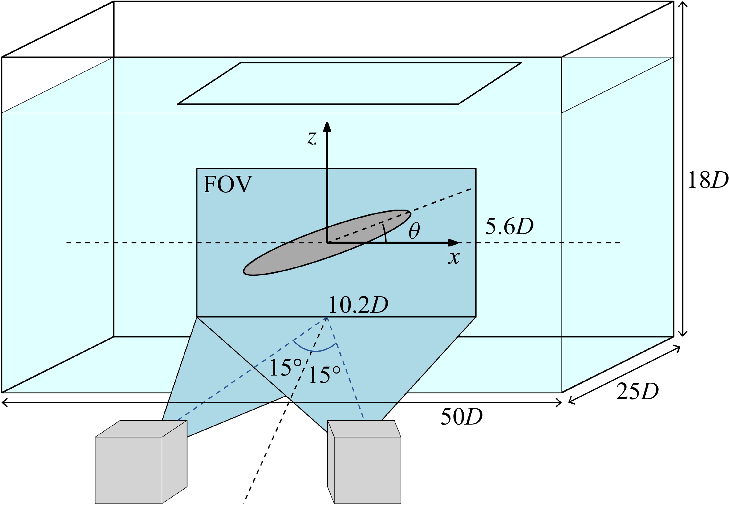


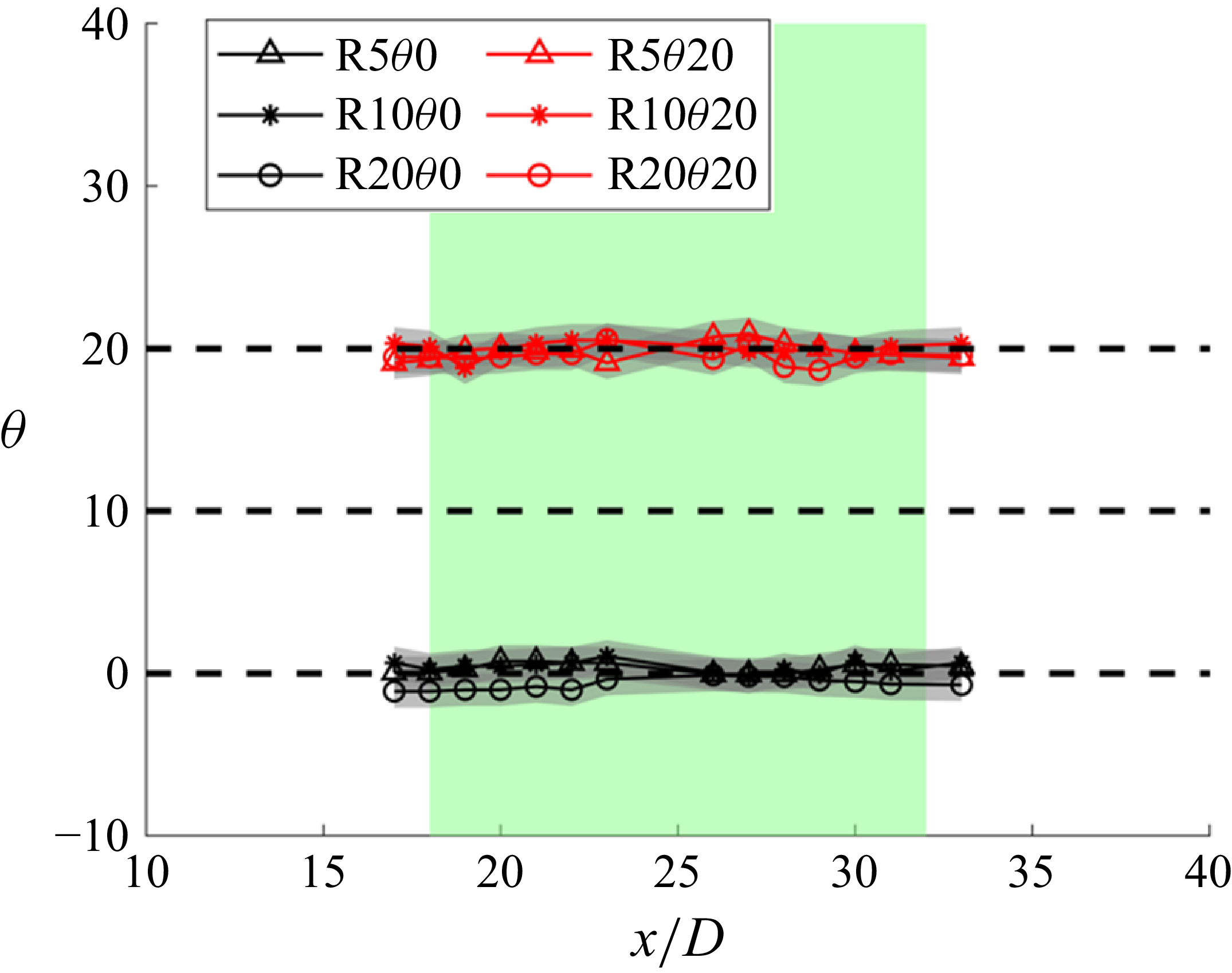
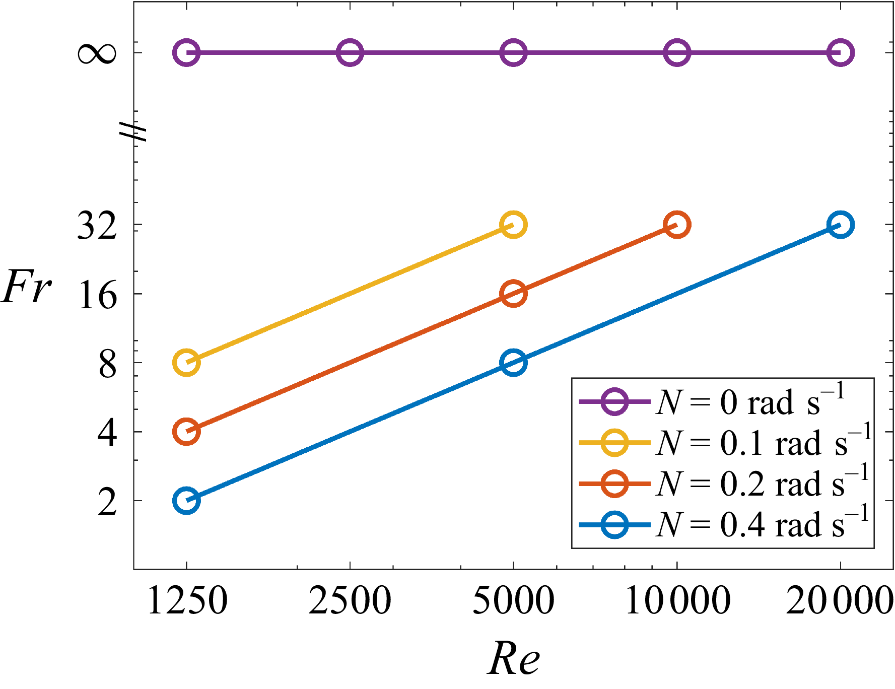


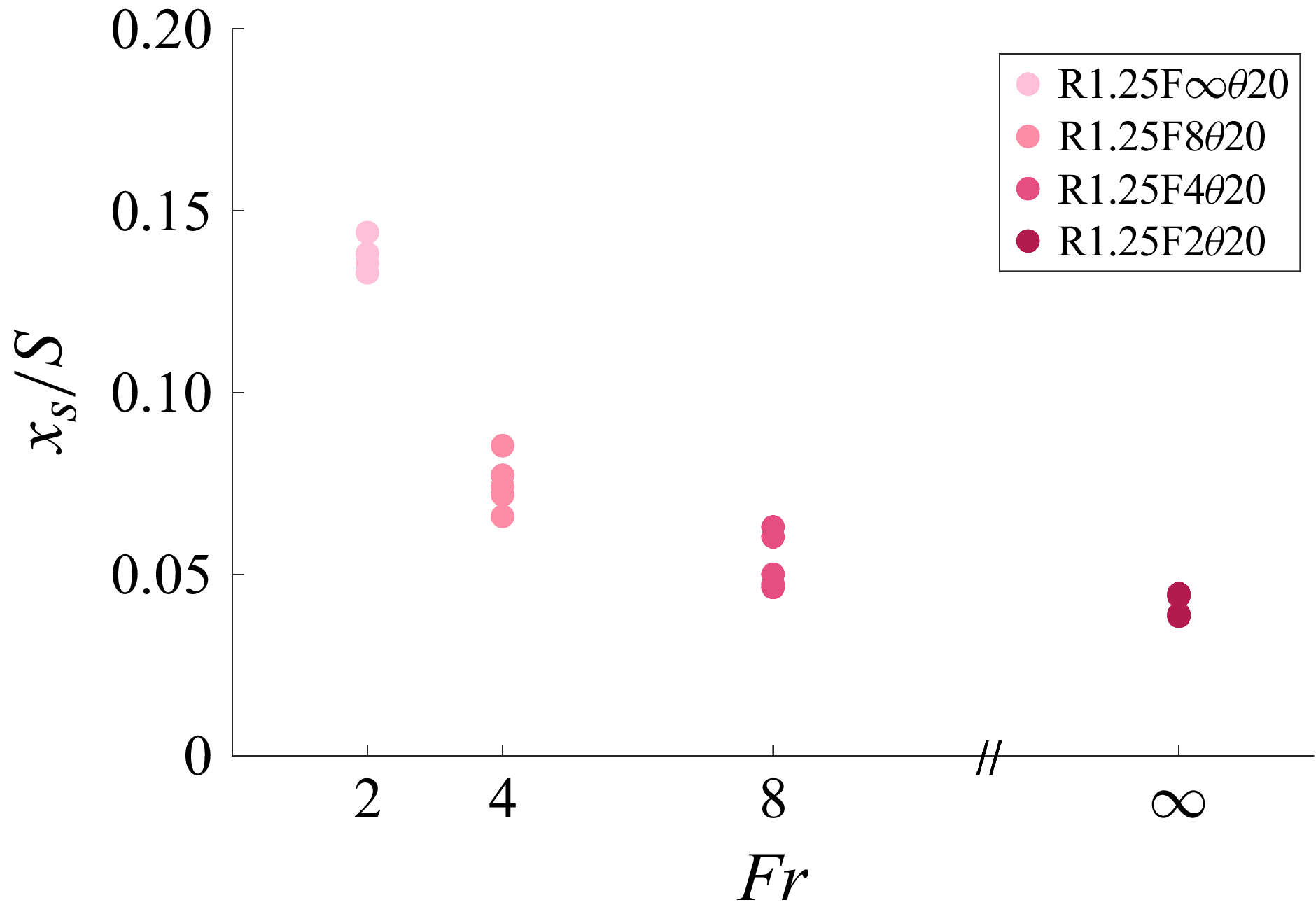


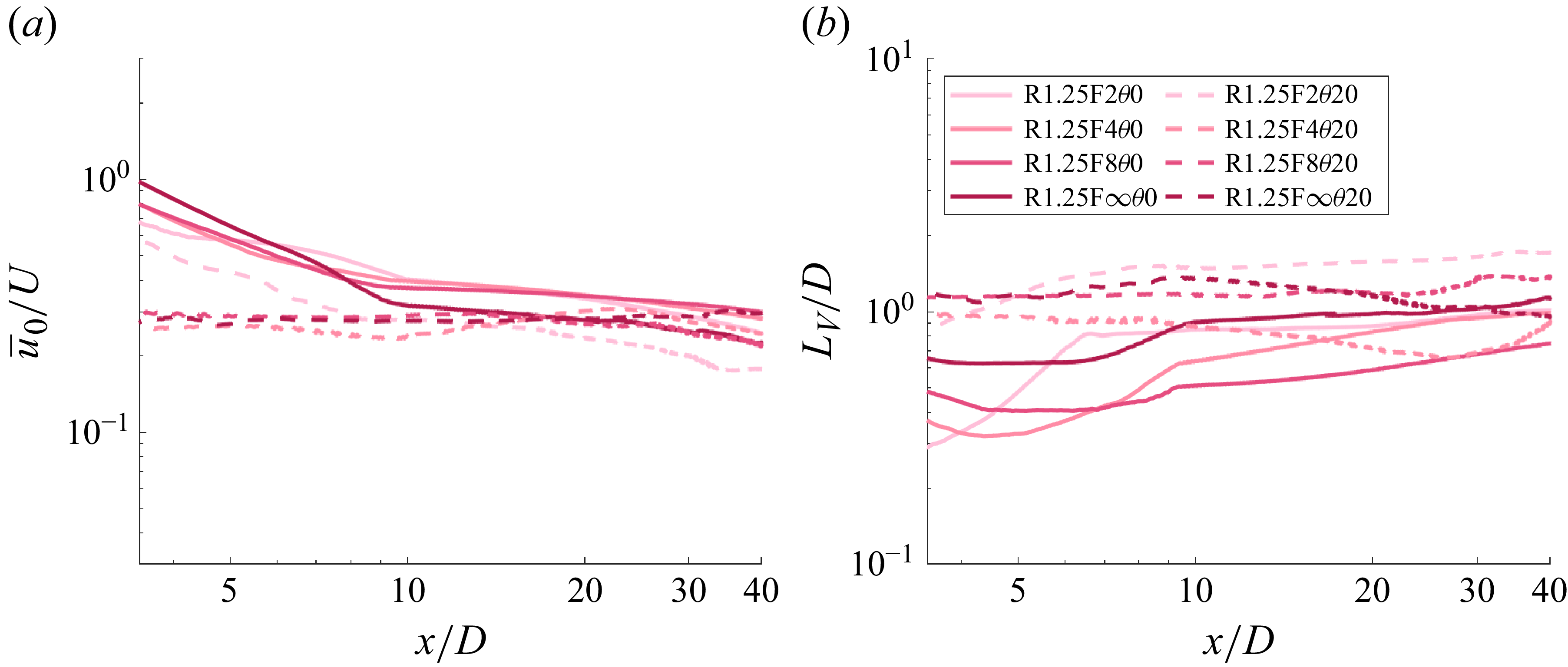


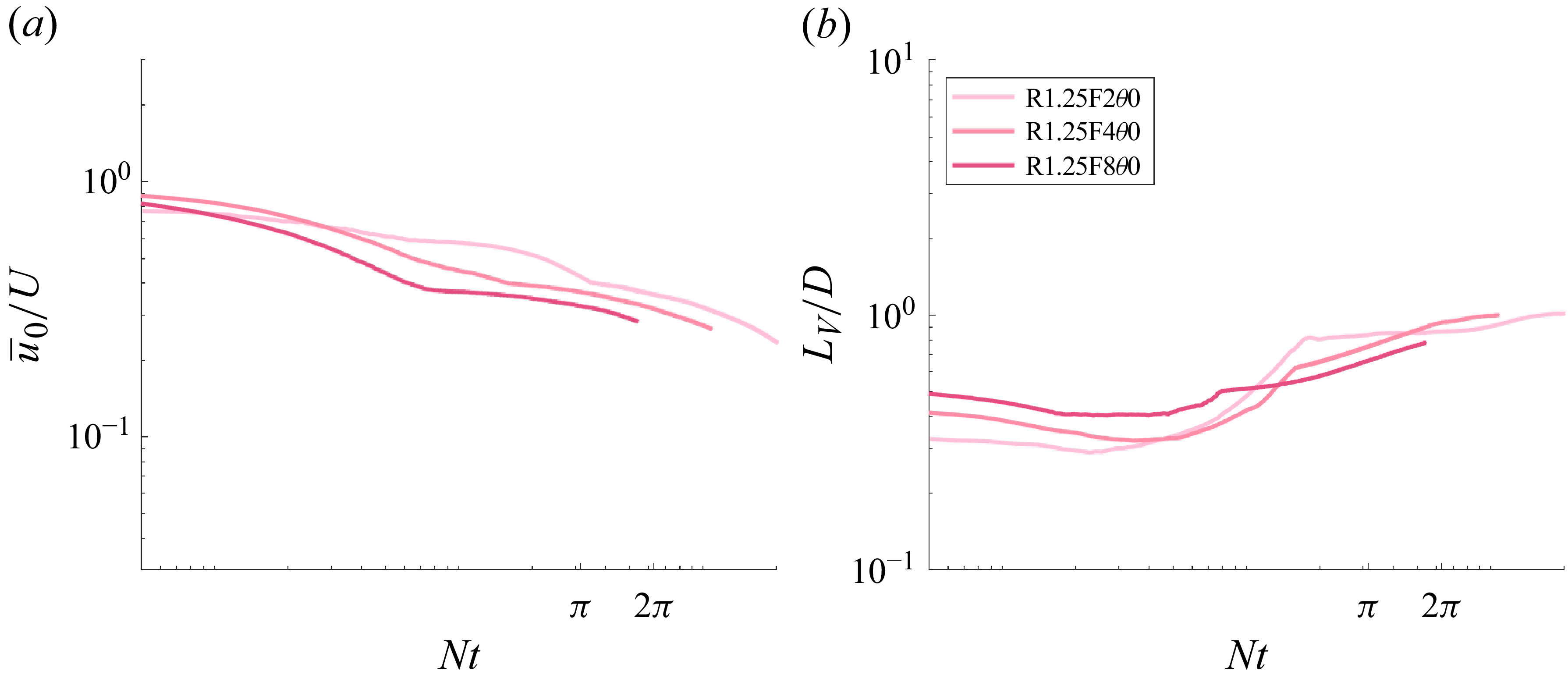


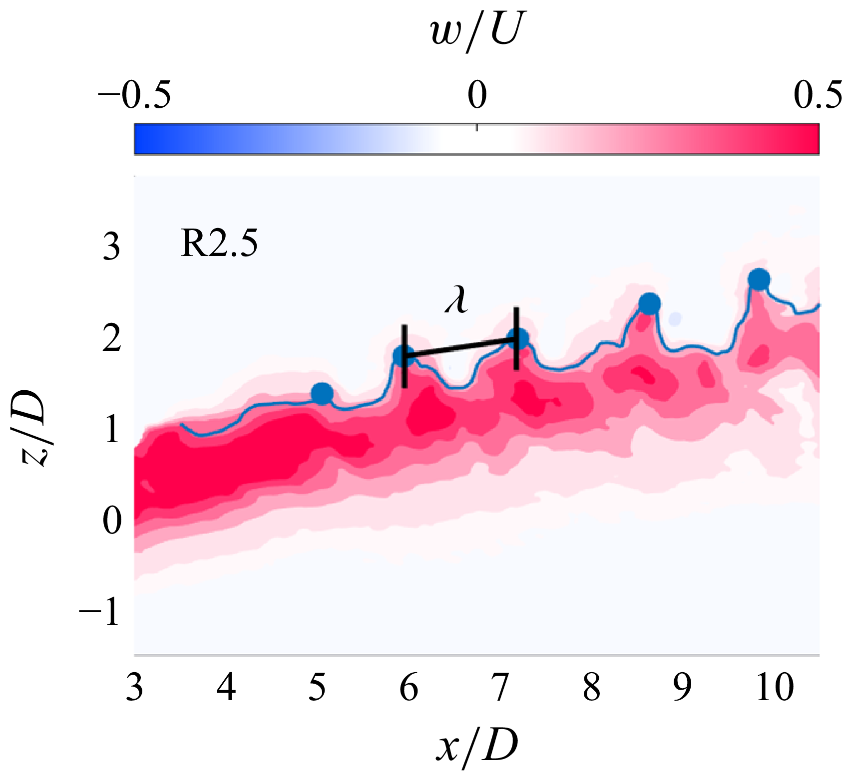


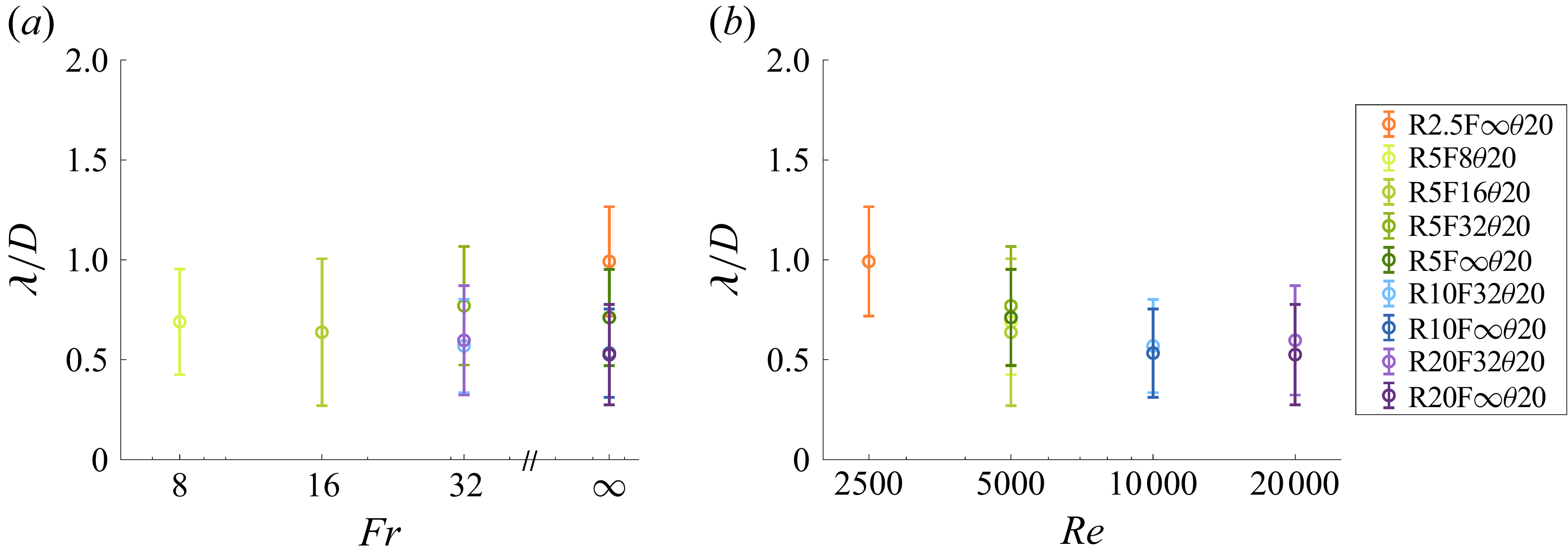


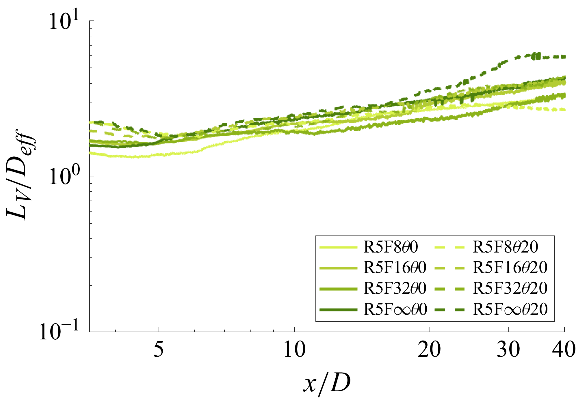


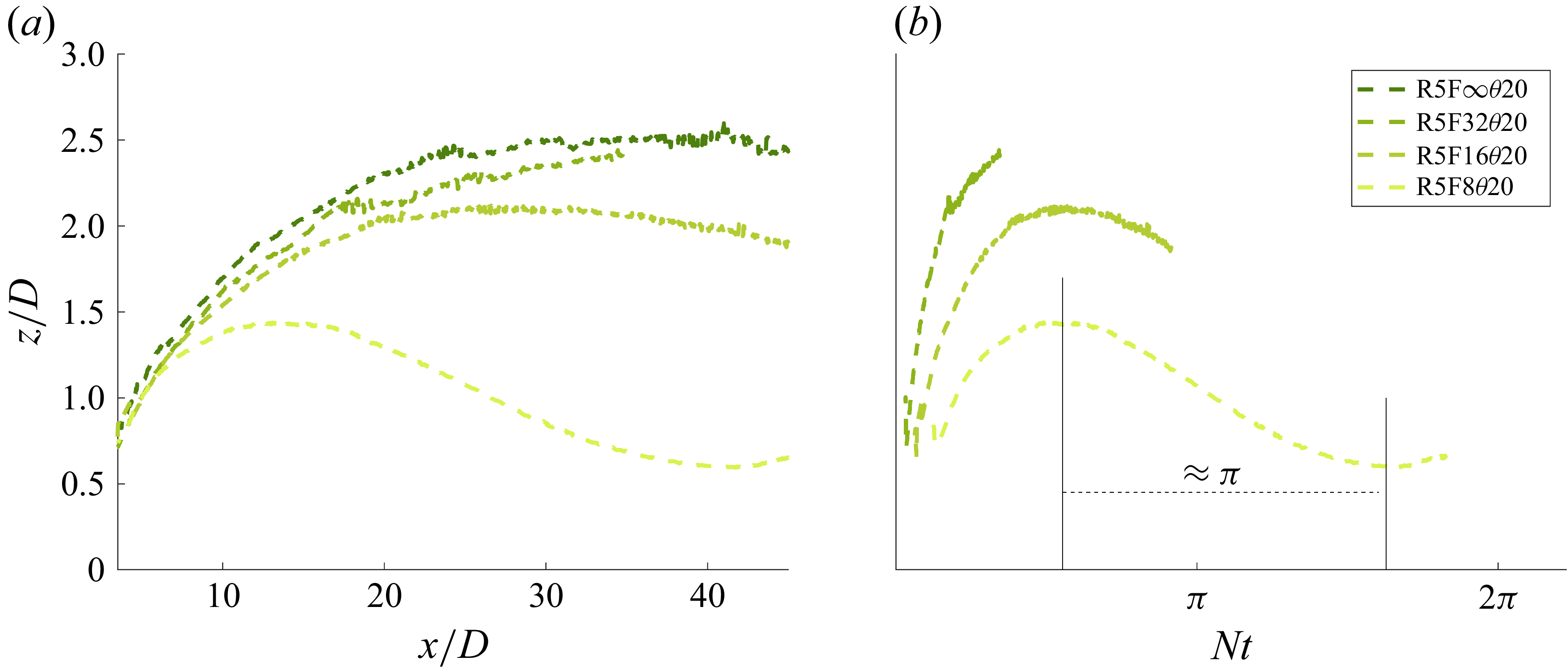


 Open access

