


Civil wars are pervading features of human society, despite their profound costs. Between World War II and the new millennium alone, there were over 70 civil wars resulting in more than 16 million deaths worldwide (Fearon and Laitin Reference Fearon and Laitin2003). These conflicts take lives, destroy property, and prevent the success of stable governments. Underlying the macro-level phenomena of civil wars are the individual decisions of millions of people to participate in these violent conflicts.Footnote 1 What leads someone to abandon the political process and take up arms against the state, risking personal life, property, and security for uncertain gains? In this article we study this question in the context of the American Civil War, one of the most destructive civil wars ever fought and “the most horrific war in United States history” (Costa and Kahn Reference Costa and Kahn2003, 520). Motivated by historical research on this defining period in America’s development and insights from conflict studies about why individuals participate in rebellions, this article investigates how personal wealth and slaveownership affected the likelihood that Southerners fought for the Confederate Army in the American Civil War. Were wealthier white Southerners—who were more likely to own slaves and therefore had higher stakes in the conflict’s outcome than poorer white Southerners—more or less likely to fight in the Confederate Army?
Research drawn from political science and history offers countervailing views on whether wealth, in various forms, should increase or decrease the propensity to fight. On the one hand, one of the most famous historical sayings about the American Civil War was that it was “a rich man’s war, but a poor man’s fight.”Footnote 2 The saying captures the claim that poorer white southern men, most of whom did not own slaves, were more likely to fight in the Confederate Army than their wealthier slaveowning peers. Such a pattern would be consistent with research in political science arguing that individuals participate in conflict in part because they gain greater material benefits from fighting than from not fighting, at least when personal wealth is not closely tied to the outcome of the conflict (Berman et al. Reference Berman, Callen, Felter and Shapiro2011; Collier and Hoeffler Reference Collier and Hoeffler2004; Dasgupta, Gawande, and Kapur Reference Dasgupta, Gawande and Kapur2017; Dube and Vargas Reference Dube and Vargas2013; Fearon and Laitin Reference Fearon and Laitin2003; Humphreys and Weinstein Reference Humphreys and Weinstein2008; Miguel, Satyanath, and Sergenti Reference Miguel, Satyanath and Sergenti2004; Olson Reference Olson1965). By this logic, wealthier southern men should be less likely to participate in the conflict, both because their wealth raises the opportunity costs to fighting and because of the potential diminishing marginal utility of money.Footnote 3
On the other hand, as we will argue throughout this article, the American Civil War was a case in which personal wealth raised individuals’ stakes in the outcome of the conflict, potentially leading wealthier Southerners to fight more despite the opportunity costs associated with their participation in the conflict. Historical work shows that free, white men of even modest means throughout the Antebellum South often invested their excess capital in land and slaves (McPherson Reference McPherson2003; Wright Reference Wright1978). The war was fundamentally fought over the institution of slavery. We might expect that as white farmers in the Antebellum South became wealthier, their incentives to preserve slavery likewise rose, possibly making them more willing to fight for the Confederacy. This logic is consistent with research throughout political science highlighting how individuals are motivated to fight due to grievances against the state (Cederman, Gleditsch, and Buhaug Reference Cederman, Gleditsch and Buhaug2013; Gurr Reference Gurr1970; Humphreys and Weinstein Reference Humphreys and Weinstein2008; Paige Reference Paige1978)—in this case, grievances against a federal government they saw as threatening an institution that they had been socialized into and upon which their future livelihood depended.
Empirical historical work that attempts to resolve this debate comes to conflicting conclusions. Studying Georgia, Harris (Reference Harris1998, 153) writes: “When men of the same age and family status (such as household head, son, or boarder) are compared, those who did not serve in the army were wealthier, and owned more slaves, than those who did serve.” Studying Mississippi, Logue (Reference Logue1993) shows that Confederate combatants were significantly poorer than non-combatants, on average (though with some areas showing the opposite). Studying Harrison County, Texas, Campbell (Reference Campbell2000) finds that wealthier individuals were more likely to fight for the Confederacy. Reviewing some of this literature, Logue (Reference Logue1993) describes these varying conclusions and discusses “obvious problems of scale in investigating enlistments” (Logue Reference Logue1993, 612). Limited to manual inspection, scholars have almost exclusively studied small samples of Confederate soldiers, often in a single county (or, in the case of Logue (Reference Logue1993), a single state).Footnote 4 The difficulties of working with samples probably explain why empirical work in this area has proved inconclusive.
To solve this problem, we take advantage of recently digitized datasets on the entire population of the Confederacy. We assemble individual-level data on roughly 3.9 million free citizens in the Confederate states alive prior to the outbreak of the Civil War. Our dataset records information about each citizen’s wealth, the number of slaves owned, occupation, family relationships, and, for men, an estimate of whether or not each fought in the Confederate Army. Using this dataset, we show that households that owned slaves fielded more Confederate Army soldiers, on average, than did non-slaveowning households. To understand these patterns—and, in particular, to gauge whether wealth and slaveownership drove people to fight for the Confederacy, or was simply a correlate of other attributes that made people more likely to fight—we present experimental evidence for the causal effect of economic wealth on the propensity to fight. Using the results of Georgia’s 1832 land lottery, which formally randomized a meaningful amount of wealth across white male citizens (Bleakley and Ferrie Reference Bleakley and Ferrie2016; Williams Reference Williams1989), we show that lottery winners’ households owned more slaves, and subsequently fielded significantly more Confederate Army members, than lottery losers’ households. These results are not merely because wealth increased the number of children in a household. Increases in wealth caused individuals to be more likely to fight for the Confederate Army 30 years later, probably in part since these increases came mostly in the form of slaves which increased the perceived stakes associated with the American Civil War.
In the final set of analyses, we try to understand why incentives to free-ride did not override the increasing stakes associated with the conflict’s threat to end the institution of slavery. Even though slaveowners as a whole had incentives to fight against the Union, any individual slaveowner would also face incentives to shirk and avoid risking death in war. We document aggregate patterns at the county-level that suggest local communities organized to encourage collective mobilization, although interpretations become inevitably more speculative. There is a strong, positive association between the county-level fighting rates of slaveowners and non-slaveowners, suggesting locality-level effects like social pressure played a role in overcoming the incentives to free-ride. The fighting rate among non-slaveowners does not increase with the prevalence of slaveowners in several Confederate states, however, suggesting that such local pressure may not have been enough to induce poor Southerners to fight in all cases.
The article contributes to the broader literature on why individuals choose to participate in violent rebellion by assessing an important historical debate in a case that continues to receive considerable popular attention but which falls in between political science’s subfields. Wealthy individuals throughout the Southern Confederacy were on average more likely to be slaveowners. Thus, the main finding of this study—that wealthier slaveowners were on average more likely to fight for the Confederate Army than non-slaveowners—demonstrates how the individuals who had the greatest stake in the continuation of the institution of slavery were the most likely to fight in defense of it. This evidence is consistent with the argument that the increasing stakes of the conflict, which threatened to end slavery, overrode the incentives for wealthy slaveowning Southerners to free-ride and avoid paying the costs of war. Although wealth may in many cases reduce an individual’s propensity to engage in violent conflict, it may increase it when it is associated with higher personal stakes in the outcome of the conflict.
WEALTH, SLAVEOWNERSHIP, AND FIGHTING FOR THE CONFEDERACY
While citizens fight in war for many distinct reasons (Levi Reference Levi1997), rational-choice models and historical accounts both indicate that personal wealth is a crucial factor that could have shaped the decision to fight for the Confederacy. Strategic models capture the individual citizen’s choice to fight as a tradeoff between the returns to his normal labor and the selective benefits of fighting (Grossman Reference Grossman1991). Historical accounts of the Antebellum South also highlight the stark economic inequalities among whites that developed in tandem with the slave economy (Merritt Reference Merritt2017). Summarizing the literature on fighting in the American Civil War, however, leads to countervailing predictions for whether wealthier individuals would be more or less likely to fight.
Before describing these divergent predictions, we first need to emphasize that the decision to fight for the Confederate Army was an actual choice. The Confederacy implemented the first compulsory draft in North American history (McPherson Reference McPherson2003, 430),Footnote 5 so it would seem at first that Southerners had little choice in fighting. In reality, there were many ways to avoid the draft. Wealthy citizens could pay to avoid service, and the draft “was not uniformly administered” (Ambrose Reference Ambrose1962, 264). Later in the war, men who owned more than 20 slaves were exempt from the draft altogether.
Perhaps more importantly, many people rich and poor simply avoided the draft. In Northwest Georgia—a region important to this article, because it is home to the land allocated through the land lottery we study later—draft dodging was so rampant that the Confederate Army was dispatched to round up reluctant soldiers (Sarris Reference Sarris2006, 88). These efforts were largely futile. Some men joined only to desert at the first opportunity; some simply refused and chose to serve time in prison; others were hidden in their homes or by neighbors; and many others melted into the woods when the army came near (McPherson Reference McPherson2003, 432). As recounted in Sarris (Reference Sarris2006, 89), W. A. Campbell, a former Confederate officer, returned home to Fannin County, Georgia, to find “a very large majority of the people now here, perhaps two-thirds, are disloyal … not 1/2 dozen men have gone into the service.” In many parts of the Confederacy, especially in areas more ambivalent toward secession, concerns that individuals could “sabotage the Confederate conscription” were widespread (Sarris Reference Sarris2006, 90). Indeed, the state government of Georgia, led by Governor Joe Brown and his lieutenant, Adjutant and Inspector General Henry C. Wayne, “obstructed conscription in every way they could” (Scaife and Bragg Reference Scaife and Bragg2004, 3).
In a landmark study on fighting in the Civil War, McPherson (Reference McPherson1997, 5) sums up how men joined the fight: “[M]ost Union and Confederate soldiers were neither long-term regulars or draftees, but wartime volunteers from civilian life whose values remained rooted in the homes and communities from which they sprang to arms and to which they longed to return.” Thus, despite the Confederacy’s best efforts to conscript soldiers, for many, the decision to fight for the Confederacy was a choice. Given this choice, how then should we expect an individual’s wealth to shape his decision to fight?
Why the Wealthy Might Fight Less: Opportunity Costs and Incentives to Free-Ride
A range of historical research on the American Civil War claims that wealthier individuals were on average less likely to fight than their poorer compatriots, in large part because wealthier individuals had both the incentives and opportunity to free-ride on their poorer southern compatriots and avoid paying the costs of war. Prior research highlights a number of historical institutions that seemingly incentivized poorer individuals to fight, while allowing wealthier Southerners to avoid it. For example, throughout the Civil War both the Confederate and Union armies used enlistment bonuses, generally known as bounties, to recruit soldiers. In early 1861, enlistees received a 10-dollar bounty (Scheiber Reference Scheiber1969, 229). Later in the year, the Confederate Congress approved a 50-dollar bounty for individuals who re-enlisted (McPherson Reference McPherson2003, 430). These bounties apparently sought to induce poor individuals to fight by increasing the monetary payoff to enlisting. The prevalence of such monetary rewards targeted toward the poor is consistent with research that argues higher levels of personal wealth make individuals less likely to participate in rebellion (Berman et al. Reference Berman, Callen, Felter and Shapiro2011; Collier and Hoeffler Reference Collier and Hoeffler2004; Dasgupta, Gawande, and Kapur Reference Dasgupta, Gawande and Kapur2017; Dube and Vargas Reference Dube and Vargas2013; Fearon and Laitin Reference Fearon and Laitin2003; Miguel, Satyanath, and Sergenti Reference Miguel, Satyanath and Sergenti2004; Olson Reference Olson1965). These authors argue that individuals participate in conflicts after weighing the material benefits they can obtain from fighting against the benefits from staying out of the conflict. In this view, wealthier individuals may be more reluctant to fight because of more valuable outside options: their regular source of income is larger than their payoff to fighting. Moreover, with diminishing marginal returns of additional wealth, the bounties would incentivize poorer individuals more than wealthier individuals.
Other conscription rules appear to have provided wealthier individuals the opportunity to avoid fighting. The rules, which angered many poorer individuals throughout the Southern Confederacy (Harris Reference Harris1998, 150), took a number of forms, including the ability to pay someone to fight in one’s steadFootnote 6 and the exemption of individuals owning 20 or more slaves from the draft.Footnote 7 These rules were explicitly set up to encourage the poor, most of whom did not own slaves, to join the Confederate Army and to excuse the wealthy from doing so. In short, wealthier individuals had the means to avoid the risks of war. This body of evidence suggests that we should expect wealthier individuals to be on average less likely to fight.
Why the Wealthy Might Fight More: Increased Stakes
Alternative arguments suggest instead that increasing wealth made Southerners more likely to fight, because southern wealth depended so heavily on the preservation of slavery. Historical accounts stress that excess wealth in the Antebellum South was overwhelmingly invested in slaves.Footnote 8 Most southern white men were farmers, and farmers by and large sought to own slaves. Surveying the economy of the Cotton South, Wright (Reference Wright1978, 141) concludes that “even the smaller [slave]holder would find his financial portfolio dominated by the value of his slave property.” Thus, for southern white men in the Antebellum period, individual increases in wealth would likely tie them even more tightly to the institution of slavery. That slavery permeated the economic decisions of the Southerns cannot be over-emphasized: “Across the South, slaveowners formed a class of great wealth with a distinctive unity of economic interest—not necessarily on policies concerning the economics of slavery, but in slavery itself” (Wright Reference Wright1978, 143).
Because the American Civil War centered on the future of slavery, Southerners who invested in this institution might perceive the stakes of a Confederate defeat to be higher than non-slaveowners.Footnote 9 Secessionists throughout the South worried a great deal about whether non-slaveowning whites would support secession (McPherson Reference McPherson2003, 242), precisely because they seemingly lacked the obvious economic motivation that slaveowners possessed. For this reason, the motivations of non-slaveowners to fight a war over slavery have long been debated. Ambrose (Reference Ambrose1962, 259) speaks of “yeomen,” small farmers without slaves, who were the majority of the southern white population, as “often unresponsive or downright hostile to their country’s cause.” A poor North Carolina woman quoted in the article wrote a letter to her governor requesting her husband be discharged from the Confederate army, writing: “I would like to know what he is fighting for…he has nothing to fight for…I don’t think that he is fighting for anything only for his family to starve” (267).
Studies of Southerners who opposed seceding from the Union further support the argument that non-slaveowners perceived the stakes of the conflict to be lower than did slaveowners. Studying the “up-country” areas of the South, where opposition was most concentrated, Tatum (Reference Tatum2000, 4) writes that “[a]lthough many of the up-country dwellers hoped some day to own slaves, they had relatively few at that time, and therefore had little to lose by emancipation.” Consistent with this claim, Wooster (Reference Wooster1977) presents evidence across the 15 secession conferences held by southern states at the beginning of the Civil War that delegates from counties with more slaves were more likely to support secession, while areas with fewer slaves were less likely to support secession. McPherson (Reference McPherson2003, 242) also observes that “[i]n the conventions, delegates supporting delay or cooperation owned, on average, less wealth and fewer slaves than immediate secessionists.” The secession, Wright (Reference Wright1978, 41) concludes, “was essentially a slaveholder’s movement.”
Such accounts suggest that wealthier Southerners were more likely to own slaves and thus perceive the stakes of the conflict to be higher than their poorer southern compatriots. Slaveowners might perceive the stakes of the conflict to be higher due to a number of factors. They likely perceived that preserving the slavery system was important to their economic well-being. Alternatively, or additionally, their direct experience of being socialized or indoctrinated into the institution of slavery increased their commitment to perpetuating it.Footnote 10 Regardless of the mechanism underpinning this stakes-based argument, we should expect slaveowners to perceive the stakes of the Civil War to be higher, and thus be more likely than poorer non-slaveholding Southerners to fight for the Confederate Army. The evidence we present is largely consistent with this expectation.
Alternative Arguments for Why the Wealthy Might Fight More
It is also theoretically important to consider alternative explanations of fighting that do not involve stakes but nonetheless predict a positive effect of wealth on fighting. For example, we might suspect that for wealthier slaveowners, their increased wealth reduced the costs associated with abandoning their farms to fight. Indeed, many in the South felt that the rich could better afford to fight. Harris (Reference Harris1998, 149) reasons that “[p]oor men and women, for obvious reasons, saw the issue of conscription in a different light from that of the rich. … [the draft] was bound to affect the families of slaveless farmers much more than those who still had someone to plow and harvest.” We might suspect, then, that slaveowners were able to rely on slave labor to offset the potential costs associated with their own absence from regular business. This would lead to wealthier individuals being more likely to fight on average, but not necessarily because the perceived stakes of the conflict had increased.
Another cost-based explanation that does not rely on stakes comes from the expectation that wealthier individuals held higher ranks within the Confederate Army (Logue and Barton Reference Logue and Barton2007, 256). If individuals with higher ranks suspect that they are on average less likely to be killed in combat, then we might expect them to have lower expected costs associated with their participation in the conflict. These perceptions of the differential costs of fighting could then make them on average more likely to fight.
We consider these possibilities empirically toward the end of this article by looking at the rates of fighting for the Confederate Army in 1861, the first year of the Civil War. Since in the early stages of the war many Southerners thought that the war would be over quickly, we might expect these costs concerns to weigh less prominently in their decision in the first year of the war. We find that wealthier individuals still fought at higher rates, even focusing on only fighting in the first year. While this by no means rules out these alternative mechanisms, the results do provide suggestive evidence consistent with the stakes-based mechanism.
HISTORICAL DATA ON CONFEDERATE CITIZENS
To test the countervailing theoretical predictions for how wealth affected individual’s propensity to fight for the Confederate Army in the American Civil War, we constructed a new dataset of nearly the entire military eligible population of the Confederacy. The dataset links three sets of publicly available sources of individual-level information: The 1850 US Census of free citizens, the 1850 Slave Schedule, and state rosters of Confederate Army membership. In the remainder of this section we outline each data source and how they were linked together.
The left panel of Table 1 summarizes our sources of data. We start from the full US Census of 1850, which contains the names for all individuals, along with their age, occupation, and place of birth.Footnote 11 We limit our analysis to the eleven Confederate states, Alabama, Arkansas, Florida, Georgia, Louisiana, Mississippi, North Carolina, South Carolina, Tennessee, Texas, and Virginia. Next, we collected the full 1850 Slave Schedules of these states.Footnote 12 The Slave Schedule records minimal demographic information for 2,574,602 slaves under the name of 263,743 owners, each of whom is identified by last name, first name (or initial), and county of residence. Finally, we gathered the state rosters for all Confederate Army soldiers in the same eleven states.Footnote 13 These rosters contain a limited set of information about soldiers including their name, state, year of enlistment or conscription,Footnote 14 and unit. This data collection effort resulted in 1,496,931 records that contain 704,650 unique state and soundex-encoded name combinations.
TABLE 1. Overview of Data Collection
Note: Each number is the number of observations for the corresponding variable. The left panel summarizes the variables captured in our raw data, with the respective source in parentheses. The right panel summarizes the counts in the dataset we construct after multiple matches. The dataset starts from the 1850 Census and then matches in data from the Slave Schedules and the Confederate Rosters by name and geography. Two specifications account for the issue of name duplicates during the merge  $- {1 \over N}$ and ${M \over N}$, and result in different estimates of the effective size of merged data. The Appendix provides detailed documentation.
We linked individuals across the three sets of data described above, starting from the 1850 Census. We declare an individual in the Census a match with a slaveowner name in the Slave Schedule if the two household head’s soundex-encoded full name,Footnote 15 state, and county are the same. Throughout, we take the unique serial number assigned to Census households in our digitized dataset as our identifier.Footnote 16 The total number of slaves is then the number of slave records associated with a Census household. Next, we link individuals in the 1850 Census to the Confederate rosters by taking all men in the Census and declare that individual a match with a Confederate roster entry if his last name, first name, and state are exactly the same in both sources, again in soundex encoding.Footnote 17 The total number of soldiers is the total number of members in any 1850 household who match to the Confederate rosters. Appendix figures illustrate the geographic distribution of our slaveownership and Confederate Army membership variables by county.
In the right panel of Table 1, we summarize the results of the matching procedure by the resulting number of observations. The key challenge is to correctly locate slaveowners and Confederate soldiers in the Census. As the fourth row shows, we are able to locate 75 percent of slaveowners in the contemporaneous Census through our matching procedure. We discuss how the remaining matching error may affect our results in the Appendix. The final row shows the result of matching Confederate names to the Census. The roster has 704,650 distinct name-state combinations, yet we join these distinct names to almost 1.4 million records in the census. The discrepancy is largely due to common names within state. We address the issue of multiple roster entries matches by creating two weighting schemes that down-weight duplicate names. The  ${1 \over N}$ column in Table 1 provides the effective number of soldiers we find in the census once we downweight each duplicated record by how many times it is duplicated in the Census (“N”). The ${M \over N}$ column does the same, except here we also up-weight the ${1 \over N}$ specification based on duplicates in the Confederate roster (“M”) as well. In the Confederate rosters, the number of name duplicates within the geographic unit is sufficiently large that we prefer either the unweighted specification or the ${M \over N}$ specification.
WHO FOUGHT FOR THE CONFEDERACY? DESCRIPTIVE FACTS
The data described in the previous section provide important individual-level information about Southern residents in 1850. In the first column of Table 2 we present key descriptive statistics about our population-based sample. The population is largely comprised of rural farmers. Households of free citizens on average include 5.5 family members, and about a fifth of all free households are estimated to own at least one slave. To examine the association between wealth and fighting, we first focus on two key pre-war measures of wealth: the number of slaves owned by an individual’s household and the value of real-estate property, both reported in the 1850 Census.
TABLE 2. Descriptive Statistics of the Two Populations Examined
Note: Summary statistics on the demographic variables. The leftmost column shows the full-count data of free citizens in the 1850 Census discussed first. The next two columns show the subset explored affected by the land lottery discussed later in the article. For these two columns the binary specification of treatment is used to separate the treatment and control; see text for other specifications. All values are from 1850.
Figure 1 presents the average number of people who served in the Confederate Army, per household, across bins of the number of slaves owned by the household. The four bins roughly correspond to the four quartiles of a household’s slaveownership. Because many households owned no slaves, the first bar represents just this subset of the data. The next three bars divide the slaveowning households into thirds.
FIGURE 1. Slaveownership and the Propensity to Fight for the Confederacy
Note: Households without slaves provided Confederate Army soldiers at a lower rate than households with slaves. The number of households in each bin indicated in parentheses. Error bars indicate 95 percent confidence intervals.
Three patterns emerge from this simple summary. First, the propensity to fight in the Confederate Army is lowest for those households owning no slaves. Second, while the jump from being a non-slaveowner to being a slaveowner predicts a large increase in army membership rates, further increases in the number of slaves are associated with more modest increases. Indeed, using a multivariate regression that includes slaveownership both as a binary variable and linearly interacted with the total number of slaves a household owns (and controls for property values), we estimate that becoming a slaveowner is associated with an increase of 0.12 soldiers, whereas conditional on owning slaves at all an additional slave is associated with an increase of only 0.017 soldiers (See Appendix). Still, both coefficient estimates are distinguishable from a null association.
Third, and perhaps most strikingly, the overwhelming majority of the Confederate Army were not slaveowners. Indeed, according to our estimates, there were more non-slaveowning households who nevertheless provided Confederate soldiers (410,646 households) than there were slaveowning households in total (193,785 households). This prevalence of non-slaveowners in the army may have led some observers to infer that non-slaveowners were just as likely, if not more likely, than slaveowners to fight. Instead, non-slaveowner’s rate of fighting in the Confederate Army was substantially lower.
Next, we consider wealth as proxied by real-estate property value—the only indicator of wealth besides slaveownership available for 1850. We again divide households into four bins, the first for non-property owners and the latter three for three terciles in terms of real-estate property wealth. Figure 2 shows that households reporting no real-estate value fought in the Confederate Army at a lower rate than those possessing some real-estate wealth. Like slaveownership, the starkest difference is between households owning no property and owning at least some property.
FIGURE 2. Real-Estate Property Wealth and the Propensity to Fight for the Confederacy
Note: Households without real-estate property wealth provided Confederate Army soldiers at a lower rate than households with real-state property wealth. Error bars indicate 95 percent confidence intervals.
The patterns apparent from the population averages are informative, but many other variables may confound the association between a household’s slaveownership (or property wealth) in 1850 and the number of soldiers the household fields a decade or more later. In the Appendix, we attempt to account for observable confounders by estimating regressions with other controls, fixed effects, and allowing for correlated errors within relevant groups. The three patterns in Figure 1 are robust to including fixed effects and clustering standard errors by last name, a proxy of the socioeconomic status of a family’s heritage, as well as to fixed effects and clustered standard errors for county.Footnote 18 The regressions also indicate that the bivariate relationship between positive real-estate wealth and fighting presented in Figure 2 may in fact be driven by slaveownership. A regression with both property wealth and slaveownership as predictors estimates the coefficient on the amount of property wealth (as opposed to whether one owns or does not own property) to be substantively close to zero.Footnote 19
In summary, our data collection and record linkage allow us to comprehensively examine the relationship between wealth and fighting, controlling for observable confounders. Wealthier households in 1850 fought at higher rates during the Civil War. Further scrutiny suggests that it is a particular form of wealth—slaveownership—that is positively associated with fighting. In the following section, we proceed to rule out unmeasured confounders by focusing on a subset of our sample that received a random shock of wealth.
WEALTH INCREASES PROPENSITY TO FIGHT: THE GEORGIA LAND LOTTERY
Did southern white men fight in the Confederate Army because they were wealthy and owned slaves, or are these variables simply correlated with other attributes that made these men more likely to fight? We now turn to an experimental design that leverages a large-scale lottery in the state of Georgia in which plots of land, worth a considerable amount of money, were randomly allocated to white men 29 years prior to the outbreak of the Civil War.
Conducted eight times during 1805–33, the lotteries were unique, widely popular among its white citizens, and covered a vast area of contemporary Georgia (Weiman Reference Weiman1991). We focus on the sixth lottery of Georgia, held in 1832, because of its outsized scale and its proximity in time to the Civil War. The 1832 land lottery, also known as the Cherokee Land Lottery, distributed Cherokee Nation territory (the northwest of contemporary Georgia) to white citizens of Georgia. The lands were forcefully taken from the Cherokees in infamous fashion, and the rights to the land became even more controversial after a gold vein was discovered in the area around 1829 and white settlers inundated Cherokee territory to strike gold. The 1832 lottery distributed land which the Georgia state legislature declared as “Cherokee County” in December 26, 1832, shortly after President Jackson won re-election. Following carefully stipulated rules set by the state legislature,Footnote 20 the surveyor office carved out land lots roughly 160 acres each to be made available to any lottery winner for a processing fee of $18.Footnote 21 Unclaimed land would eventually return to the ownership of the state of Georgia.
After eligible citizens registered for the lottery by sending their names to the governor’s office in Milledgeville, Georgia, commissioners conducted the lotteries in a doubly-randomized process (Williams Reference Williams1989). Lottery organizers set up two large drums called “wheels.” One wheel for names contained slips of paper for every registrant for the lottery. The second wheel for land contained a slip of paper for every parcel of Cherokee Nation land up for lottery. Commissioners simultaneously drew one slip of paper from each of the two wheels, so that both whether or not a person won the lottery, and the exact location of the land were randomized. Eligibility requirements remained roughly consistent across all eight lotteries. Household heads 18 years or over, with a minimum three-year residence in Georgia and US citizenship, were all covered (Georgia Archives 2018). Winners of previous lotteries were excluded. Certain groups, most notably those with a spouse and children, were advantaged by having two draws at the lottery.
While the lottery distributed wealth in terms of land, its practical effect was to increase the winner’s monetary wealth that could then be used for other purposes. Historical evidence suggests that richer citizens eagerly bought off lotteried land from winners of the lottery, effectively creating a private market for land. Indeed, “Even mediocre land could probably be sold for $25 or $50, probably enough to exempt [a yeoman household head who won the lottery] from ever paying taxes again … If he hit the jackpot and won a piece of prime cotton land worth several hundred dollars, then he could quickly rise up the ranks and perhaps even buy a slave” (Weiman Reference Weiman1991, 857).
Identifying the Winners and Losers of the Land Lottery
To analyze the lottery, we first use a digitized dataset of lottery winners’ names (Smith Reference Smith1838), which includes their self-reported place of residence and a symbol for whether the winner paid the fee and claimed the land he won at the time of publication. This results in information on 18,219 unique individuals. The records of lottery winners are an official census (not self-reported), “all carefully copied from the originals in the Executive Department and the office of the Surveyor General, designating also the lots which have been granted” (Smith Reference Smith1838, iii). We will then define our experimental population as a specific subset of the 1850 Census which reasonably could have entered the lottery and had the same number of draws. Finally, we seek the names of the lottery winners among this subset of predicted entrants.
Identifying the counterfactual lottery losers is key to examining the causal effect of winning the lottery. In an ideal world, we would obtain the entire population of lottery entrants and then directly compare those that lost with those that won. Unfortunately there is no available list of state-wide lottery losers; instead, we adopt the same method used in recent research conducted in economics on the monetary and educational effects of the same land lottery (Bleakley and Ferrie Reference Bleakley and Ferrie2016). We identify a subset of individuals who were eligible for exactly two draws from the land lottery in the 1850 Census, using a set of pre-treatment characteristics that all but ensures the individual was eligible. Because the lottery was popular and estimates suggest more than 97 percent of those eligibles entered (Bleakley and Ferrie Reference Bleakley and Ferrie2016, Appendix A), we then assume that such eligibles entered the lottery, or at least are equivalent in their pre-lottery characteristics and potential outcomes to those who entered and subsequently won. Specifically, starting from the same observational dataset from the previous section, we take all male household heads born before 1814 who had a child (alive in 1850) in Georgia between 1829 and 1832. Individuals who we find in the list of winners are labeled as treated, while those that do not match we label as control. In the Appendix, we show that treated and control households are similar in terms of the pre-treatment characteristics we are able to measure.
Astute readers will notice at this point that we are defining our counterfactual pool (1832 lottery losers) using post-treatment observations (1850 Census observations). In line with the empirical strategy presented in Bleakley and Ferrie (Reference Bleakley and Ferrie2016), we assuage these concerns in two ways. First, because we use a full-count dataset of the entire Southern United States, outcomes are observed even for individuals who moved away from Georgia. Second, treatment could affect individual wellness or longevity, so that lottery winners are more likely to still be alive and in the Census in 1850 than lottery losers. The resulting comparison among surviving lottery winners and losers could then be biased if, for example, the subset of losers who are still alive in 1850 are those who for other reasons became wealthier or higher status. We suspect this issue is relatively minor because the treatment was not so large as to affect longevity dramatically. Nevertheless, in order to address this concern, we also applied our assignment mechanism to the 1830 Census, finding similar rates of treatment assignment. Although the 1830 Census is not digitized to an extent that we can test our specific hypotheses, retrieving similar aggregate match rates from a pre-treatment dataset is encouraging evidence that treatment did not affect longevity in a way that would subsequently affect our estimates.
We identify lottery winners by computing the phonetic distance of both first and last names between the two data sources. This metric allows us to sidestep potential issues involving variation in spelling, transcription errors, and enumerator spelling errors, which might lead the same individual to have his name spelled slightly differently in the 1832 winners’ list and the 1850 Census.Footnote 22 Traditional exact matching will falsely declare such cases as negative matches. We use a phonetic distance metric informed by the historical evolution of languages, implemented in the R package alineR (Downey et al. Reference Downey, Hallmark, Cox, Norquest and Lansing2008; Downey, Sun, and Norquest, Reference Downey, Sun and Norquest2017). We declare two names a match if the “aline” distance of the first and last names are both less than 0.05 (where distance ranges from zero to one).
To account for multiple matches, we consider three specifications of treatment status based on this phonetic distance metric, roughly equivalent to our procedure in the construction of our observational dataset. In the binary specification, we assign the treatment indicator by examining whether a name in our eligible population corresponds one-to-one with a name in the lottery winners’ list. The  ${1 \over N}$ [following Bleakley and Ferrie (Reference Bleakley and Ferrie2016)] and ${M \over N}$ specification attempt to account for duplicate names by down-weighting multiple matches. These three specifications identify treated individuals among the eligible population with a range of coverage. The ${1 \over N}$ specification generates a 19 percent treated sample, whereas the binary specification gives 15 percent and the ${M \over N}$ specification gives 26 percent.
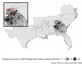
All of this leaves us with 13,414 individuals (or about 2.6 percent of the population of Georgia in 1830) from the Census. These individuals combined with their 1850 household members amount to 106,300 individuals (or about 2.7 percent of the southern free citizens) in our dataset. Figure 3 presents the geographic distribution of these eligible individuals across the Antebellum South in 1850. The center and right columns of Table 2 introduced earlier compares the demographic characteristics of this sample, separated by the binary treatment indicator. The sample of lottery entrants are understandably concentrated in Georgia, although nearly a quarter of them are estimated to have moved to another state by 1850.Footnote 23

FIGURE 3. Distribution of Inferred Lottery Entrants in the 1850 Census Analyzed
Note: The map counts the number of 1850 Census household heads per county who we identified as lottery entrants in 1832 (A strict subset of the total lottery entrant population). Counties outlined in the inset graph outlines former Cherokee county, the ownership rights of which the Georgia state government distributed by lottery in 1832. Most lottery winners’ households are still concentrated in Georgia 18 years after the land lottery, though some households have moved west.
Among the winners we examine, 48.4 percent were recorded as having claimed the land. The relatively low uptake is likely due to the variation in land values and the market dynamics described earlier. Accounts of the implementation of the lottery finds that spectators and mining companies were keenly aware of the value of the particular lots of land being lotteried away. As soon as the state announced the winner for a valuable lot, these buyers flocked to give their bids (Williams Reference Williams1989). In contrast, citizens who won less valuable land, despite winning the lottery, perhaps felt it was not worth even the fee to claim the land (Weiman Reference Weiman1991, 842). The state extended the deadline for a winner to claim their land several times, further incentivizing winners to wait for a favorable offer.
Estimation
Our experimental analyses compare 1850 household members whose household head won the 1832 land lottery to 1850 household members whose household head reasonably entered the 1832 lottery but lost. The randomized nature of the lottery allows us to estimate causal effects at the household level using a simple OLS equation of the form
 $${Y_i} = {\beta _0} + {\beta _1}\;Won\;Lotter{y_i} + X_i^ \top \gamma + {\varepsilon _i},$$
where Y i is an outcome variable for household i. The treatment of the 1832 father winning the lottery, denoted by Won Lottery i, is also realized at the household level. This variable stands in for any of the three treatment variable specifications discussed above. The vector X i stands in for an optional vector of control variables. The coefficient β 1 estimates the average effect of winning the lottery. Because 52 percent of those who won did not claim, the coefficient represents a dilution of the average effect of actually reaping the benefits of winning the lottery. In the following analyses we present estimates of winning the lottery (β 1), but note that the estimated effect of wealth among those who actually consumed it is roughly twice that of β 1, computed by instrumenting the choice to claim with the randomized result of the lottery.Footnote 24
EFFECTS OF RANDOMIZED LAND LOTTERY ON SLAVEOWNERSHIP AND FIGHTING
We now present experimental estimates on both slaveownership and fighting.Footnote 25 We find a large positive effect of winning the land lottery on slaveownership at the household level. The first two panels of Figure 4 show that households whose fathers won the 1832 lottery had on average 0.94 more slaves in 1850, and were 6.4 percentage points more likely to own slaves at all, compared to households whose fathers did not win. This represents a substantial difference in the number of slaves owned by individuals who won the lottery compared with those who lost. Substantively, this provides direct evidence supporting accounts of individuals throughout the Antebellum South investing their newly acquired wealth in purchasing slaves.

FIGURE 4. 1832 Lottery’s Effects on Slave Wealth and Real Estate Property Wealth in 1850
Note: Winning the land lottery increased both the average number of slaves a household owned, and the proportion of households that owned at least one slave. In contrast, the land lottery’s effects on overall wealth seem to be driven by slavery wealth, as there is no discernible increase in real-estate wealth. Each panel shows the estimated means for a given dependent variable, among each treatment group. Error bars show 95 percent confidence intervals using robust standard errors.
The next two panels of Figure 4 show modest effects on the amount of real-estate property wealth owned by individuals who won the Georgia land lottery as recorded in the 1850 Census. We find that average household real-estate value in the Census was roughly $150 higher for lottery winners than for lottery losers. In contrast, the proportion of households with any property wealth is approximately the same for lottery winners and losers. These modest effects on real-estate wealth again suggest that most excess capital was invested in slavery. Indeed, Bleakley and Ferrie (Reference Bleakley and Ferrie2016) estimate a meaningful effect of the lottery on total wealth, and they find that these effects are primarily concentrated in slavery rather than real estate. Like southern white men more generally, winning families in our sample appear to have invested much of their newfound capital in slavery.
Next, we trace these effects through to fighting in the Confederate Army. Figure 5 shows our main result, demonstrating that households whose fathers won land in 1832 on average had 0.3 more men fight in the Confederate Army, and were roughly four percentage points more likely to have a male household member fight in the army at all. The point estimates are substantively large and statistically distinguishable from zero.
FIGURE 5. 1832 Lottery’s Effects on Confederate Army Membership in 1860s
Note: Winning the land lottery increased both household’s average number of men in the Confederate Army (both as an average count and as a fraction of men in the household) as well as the proportion of households containing at least one soldier. Each panel shows the estimated means for a given dependent variable, among each treatment group. Error bars show 95 percent confidence intervals using robust standard errors.
Table 3 presents our main results across specifications.Footnote 26 The first column in the top panel shows the estimated effect on the average number of Confederate soldiers in the household, for the binary and  ${1 \over N}$ treatments, respectively. This estimate shows that winning the lottery led to an average increase of 0.3 in the number of soldiers in the household who fought for the Confederate Army.
TABLE 3. Effect of Winning 1832 Lottery on Household Confederate Army Membership
Note: Each cell is a regression coefficient. Sample size in all regressions is 13,414 households. Robust standard errors in parentheses. Outcome variable in top panel is the number of registered Confederate soldiers in the household. Outcome variable in middle panel is fraction of sons in household who fight in Confederate Army. Outcome variable in bottom panel is indicator for whether at least one son in household fights in Confederate Army. Columns indicate the use of fixed effects (FEs). Estimates in first row of each panel use the binary treatment indicator based on unique name matches. Estimates in second row of each panel include non-unique name matches, where the treatment variable takes the value  ${1 \over N}$ for a lottery winner name matched to N households in 1850 Census.
We also estimate the same quantity with fixed effects for the last name, or with fixed effects for the first name, following Bleakley and Ferrie (Reference Bleakley and Ferrie2016). The purpose of these name-based fixed effects is twofold. First, they address concerns that results are driven by the conduciveness of certain names to match across data sources. Second, they also account for unobserved confounders that vary across lineages, which are proxied by name. The second column of Table 3 adds fixed effects for soundex-coded household head’s last name as in Bleakley and Ferrie (Reference Bleakley and Ferrie2016); in the final column, we instead use fixed effects for soundex-coded household heads’ first names. In both cases, estimates are roughly unchanged.Footnote 27 The middle and bottom panels repeat these same specifications for our alternative outcome variables—the probability that at least one male member fought (middle panel), and the fraction of free men who fought in the Confederate Army (bottom panel). Again, we find consistent and large results.
The outcome measure in the bottom panel is particularly important because it helps refute an alternative, fertility-based explanation of our findings. Wealthier households might simply have had more sons, and therefore more chances to field soldiers. Winning the lottery indeed increased fertility, as Table 4 shows. While the lottery’s average effect on household size is smaller in magnitude than the fighting effects in the top panel of Table 3, directly addressing the extent to which this alternative mechanism is driving our results requires some care because fertility is an intermediate outcome (in 1850) between the treatment (in 1832) and the main outcome of interest (between 1861–65). We therefore assess the lottery’s effects on the propensity of fighting, measured by the number of soldiers as a proportion of the household’s total number of men. These specifications still show positive effects on fighting. As a share of all men in each family, winning households’ male members joined the Army at a rate roughly six percentage points higher than that of losing households’ male members. We also re-estimate the model controlling for household size directly, while acknowledging that this may induce some additional post-treatment bias (Rosenbaum Reference Rosenbaum1984). Estimates of the lottery’s effect on the number of soldiers for the average-sized household presented in the Appendix are attenuated by about 20 percent but remain statistically distinguishable from zero, and our results for other two outcome measures are virtually unchanged.
TABLE 4. Effect of Winning 1832 Lottery on Fertility
Note: Each cell is a regression coefficient with the number of sons as an outcome, and formatted in the same way as Table 3. Sample size in all regressions is 13,414 households.
Taken together, the experimental evidence bolsters our observational findings, and further suggests that wealth increased the propensity for Southerners to fight in the Civil War because it led them to become slaveowners. On average, lottery winners used their newfound wealth to buy slaves, and not to invest in more real estate. As a result, when war broke out, winning households were more invested in the war’s outcome than were losing households, and they fought at higher rates. While other forms of wealth not contingent on a conflict’s outcome may only raise opportunity costs and not encourage fighting, wealth that a conflict directly threatens appears to lead individuals to fight at higher rates.
DIFFERENTIAL COSTS AS AN ALTERNATIVE MECHANISM
The stakes-based mechanism is not the only way through which wealth, translated into slaveownership, might increase the propensity to fight. As we have discussed in our theoretical overview, one alternative potential explanation is differential costs: the opportunity costs from abandoning regular business might be lower for slaveowners than for non-slaveowners. In addition, if wealthier slaveowners estimate the costs of participating in conflict to be lower because they would enter the military at higher ranks than their poorer southern compatriots, this would also lead to a positive effect of wealth and slaveownership that does not operate through heightened stakes.
In order to better understand whether differential costs are solely responsible for the effect we observe, we limit our attention to 1861, the first year of the war, before the Confederacy officially began conscription on May 16, 1862. At the onset of the conflict, many people on both sides of the conflict believed that the war would be both short and easy, likely lasting just a few battles. This sentiment is captured by the writings of an Alabama soldier fighting for the Confederate Army, who asserted, in 1861, that the war would be over by the next year since “we are going to kill the last Yankey before that time if there is any fight in them still” (McPherson Reference McPherson2003, 333). Given this sentiment, we should expect individuals who joined the Confederate Army at conflict onset to be less concerned about the costs associated with leaving their farms unattended for extended periods of time, since they expected to be home again by the following year. Moreover, this optimism at conflict onset would lead individuals selecting into the military to perceive the costs of fighting to be low. As one Mississippian put it, he joined the Confederate Army “to fight the Yankies—all fun and frolic” (McPherson Reference McPherson2003, 332). Many volunteers at the war onset enlisted in contractual obligations “which ranged from three months to one year” (Levi Reference Levi1997, 62). We expect that in this first year of war, individuals would be less concerned about the costs associated with leaving their farms unattended, since they expected to be home again by the following year.
Based on this logic, if this differential cost argument were correct, we might expect to observe a smaller or null effect of winning the lottery on fighting in 1861. However, we find that winning the lottery caused higher rates of fighting even in 1861 (Table 5); in fact, the point estimate is a bit larger for 1861 than for subsequent years. While this does not conclusively rule out the possibility that differential costs affect the choice of fighting for the Confederate Army, it does lend support to the argument that slaveowners were more likely to fight because they perceived the stakes of the conflict to be higher.
TABLE 5. Effect of Winning 1832 Lottery on Fighting at Different Stages of the Civil War

Note: Each cell is a regression coefficient. All specifications do not use fixed effects and use the  ${1 \over N}$ treatment specification.
Lottery effects on fighting throughout the War are similar compared to the fighting only recorded in 1861. Each pair of columns compare the effect of winning the 1832 Lottery on one of the three metrics of army membership, corresponding to the panels in Table 3. The comparison is between fighting for all years (as already presented in Table 3) versus fighting only in 1861, as recorded by the roster record.
DID LOCAL COMMUNITIES ENCOURAGE FIGHTING?
Having laid out both observational and experimental evidence for the causal links between wealth, slaveownership, and fighting in the Confederate Army, we now turn to more speculative evidence for how and why the stakes of the conflict associated with the potential end to the institution of slavery overrode the incentives for the wealthy to free-ride and avoid paying the costs of war. Although we have explained why owning slaves might cause individuals to perceive the stakes of the conflict to be higher, the results do not directly reveal why any individual actually chose to fight. For any one individual, the risk of death in war would seem to make joining the Army fundamentally at odds with self-interest, no matter the increased stakes.
Historical accounts suggest that local communities organized together to encourage white southern men to fight, while also isolating and punishing shirkers.Footnote 28 Sarris (Reference Sarris2006, 52) describes for example how in Georgia, “communities rallied to support the soldiers,” offering “parades and public displays supporting their departing soldiers, ceremonies that were designed to reinforce the commonality of interests among the men, women and children…” The account continues, “Indeed, one of the first acts of the secession convention was to establish a formal definition for treason. Confederate loyalty was a statewide obsession…” (Sarris Reference Sarris2006, 57). As the main supporters of secession, slaveowners were at the center of these efforts. By contrast, in many areas, poor, non-slaveowning whites had been against secession (Merritt Reference Merritt2017, 300). Being wealthier and more prominent in their communities, slaveowners likely found it harder to shirk. Contributing soldiers to the war effort may have been only one out of the many ways slaveowners worked to induce other Southerners to fight.
To investigate the possibility of community-level mobilization, we compare fighting rates among slaveowners and non-slaveowners across geographical contexts, aggregating household-level information on slaveownership and fighting for each of the 692 counties. If the decision to fight were driven by contextual factors beyond an individual’s slaveownership, the fighting rate of non-slaveowners and slaveowners would be positively correlated. In contrast, if slaveowners and non-slaveowners coordinate their behavior separately, their rates of fighting may be uncorrelated, and if wealthy slaveowners compelled non-slaveowners fight while avoiding fighting themselves, the two rates may be negatively correlated.
Figure 6 plots these two quantities and exhibits a tight correlation of 0.82. In counties where more non-slaveowners fight, more slaveowners fight, too. Consistent with our main findings, slaveowners also fought at higher rates than the non-slaveowners in their own counties, as the clustering of points above the 45-degree line makes clear. These relationships exist within each of the eleven states, suggesting the pattern is not driven simply by differences between states. While wealth in the form of slavery encouraged individual households to fight, contextual factors likely played a widespread role as well.
FIGURE 6. County-Level Fighting Rates of Slaveowners and Non-Slaveowners
Note: Each point is a county’s rate of fighting in the Confederate Army among non-slaveowning households, compared to the county’s fighting rate among slaveowning households. A 45-degree line, which would denote that slaveowning and non-slaveowning households fought at equal rates, is added for clarity. The two are tightly correlated, suggesting community-level factors. Slaveowning households fielded more Confederate soldiers than the non-slaveowning households in the same county, consistent with our main findings.
Was the prevalence of slavery, and thus the prevalence of households with higher stakes in the war, one such contextual factor? If local community pressure had induced both slaveowners and non-slaveowners to fight, then counties with more slaveowners ought to be more effective at inducing non-slaveowners to fight, all else equal. The caveat is that with observed fighting rates at the county-level, our average non-slaveowner may vary in various unobservable ways in counties with different prevalence of slaveowning households.
The relationship between a county’s slaveownership and its fighting rates among non-slaveowning households are shown in Figure 7. As the figure shows, this relationship varies considerably across states. In Florida, Louisiana, and Texas, non-slave owning households were more likely to fight in counties with more slaveowners (in 1850). But in Arkansas, North Carolina, and Virginia—states in the mountain south where historians have documented opposition to the Civil War—non-slaveowners appear less likely to fight as the prevalence of slaveowners in their states increase. If the high stakes in the war’s outcome compelled slaveowners to engage in community pressure to increase war participation, its effectiveness may have not been sufficient to overcome the poor’s disincentive to fight in a number of key states.
FIGURE 7. Fighting Rates for Non-Slaveowners Across County-Level Slaveownership Rates
Note: Each county is plotted twice: the estimated proportion of men in non-slaveowning households who fought (in solid white points, with linear fit overlayed) and the estimated proportion of men in slaveowning households who fought (in gray points). In the northern Confederate states of Arkansas, North Carolina, and Virginia, counties with more slaveowners had fewer proportion of non-slaveowning men fighting. In the southern states of South Carolina, Louisiana, Florida, and Texas, counties with more slaveowners had a larger proportion of slaveowning men fight. States ordered by the magnitude of the slope coefficient of slaveownership on non-slaveowning fighting rates, printed at the bottom of the graph.
A full account of how locality-specific forces compelled slaveowners and non-slaveowners to participate in the conflict is beyond the scope of this article. However, in this section we have presented suggestive evidence that social forces beyond an individual household’s perceived stakes in the war were at play. These forces may have helped to translate individuals’ perceived stakes into costly behavior.
CONCLUSION
In this article, we have explored how individual wealth, in the form of slaveownership, affected the likelihood Southerners fought for the Confederate Army in the American Civil War. We have found consistent evidence that slaveownership increased individuals’ propensity to fight—in contrast to patterns found in previous research studying other conflicts and other kinds of wealth—because it was a form of wealth directly threatened by the war. Wealthy slaveowners who perhaps would have avoided fighting in other conflicts fought at higher rates in the American Civil War because the stakes of the conflict were high for them.
We developed two main empirical strategies to arrive at this conclusion. In the first, we used data on almost every citizen of the Confederacy to show that slaveowners fought in the Confederate Army at higher rates than non-slaveowners. To understand whether these observational patterns were causal, in the second approach, we then focused on a randomized lottery run by the state of Georgia. We showed that the households of lottery winners owned more slaves, and, perhaps as a consequence, were more likely to have sons fight in the Confederate Army.
Our findings speak to the old saying that the Civil War was a “rich man’s war but a poor man’s fight.” In some sense, this saying is accurate. The Confederate Army was majority comprised of non-slaveowning individuals. On the other hand, we found that slaveowners fought at higher rates than non-slaveowners, and that relatively modest increases in wealth and in slaveownership made southern white men more likely to fight, not less. The familiar observation that many soldiers were non-slaveowners largely reflects the fact that most Southerners were not slaveowners, but it does not imply that non-slaveowners supported the Confederacy more enthusiastically—in fact, non-slaveowners were measurably less enthusiastic.
In addition to helping shed light on historical understandings of the Antebellum South and Confederacy, our findings highlight potential areas for subsequent investigation. Future research could more explicitly theorize and empirically test the circumstances under which individual perceptions of the increasing stakes of a conflict overcome the incentives to free-ride. While our results indicate that the Confederate South was one such case, the same may not hold in other contexts with different historical features. For example, in cases where social pressure is less effective—the Confederacy was, arguably, an unusually martial culture that placed a particularly high value on military service, making social pressure a strong mobilizing force—the community links driving both rich and poor alike to fight might be less operative. This might make it easier for wealthy individuals to pay people to fight in their stead and also reduce their incentives to enlist in order to encourage poorer community members to fight alongside them.
We also hope that this article demonstrates the benefits of linking the study of conflict to the study of American politics and history. Perhaps because America’s internal violent conflicts fall into an unclear zone between the fields of American Politics, Comparative Politics, and International Relations, the subject often seems neglected. But the violent conflicts of America’s past have much to teach political scientists, both about conflict and about American political development. Moreover, as demonstrated by our ability to gather individual-level information on roughly 3.9 million Confederate citizens for this study, new efforts by archivists and genealogists offer unprecedented ways to study American political history on a comprehensive scale. In our view, this represents an opportunity to study fundamental questions about individual-level decision-making in key historical moments at both a scope and level of detail not previously possible.
The American Civil War was an incredibly destructive conflict, fought over a singularly horrifying institution, slavery. As other research shows, the ideas and motivations shaping why Southerners fought for the Confederacy did not die when the Civil War ended; they may have played a central role in shaping the long-run development of modern America (Acharya, Blackwell, and Sen Reference Acharya, Blackwell and Sen2018; Key Reference Key1948). Understanding why individuals would willingly risk their own lives to fight to preserve slavery remains an important question, so that we can understand the conditions under which political extremism does or does not lead to violent conflict. No doubt, there are many explanations, and no single answer. In this article, we have used large-scale data on the Confederacy to shed light on one key component of the answer: the economic reality of individual stakes in the institution of slavery. Contrary to some conventional wisdom, wealthier people joined the Confederate Army at higher rates than poorer people, probably because they had the most to gain from preserving a system of slavery that prioritized their own well-being over the freedom and well-being of others, and the most to lose from the system’s destruction.
SUPPLEMENTARY MATERIAL
To view supplementary material for this article, please visit https://doi.org/10.1017/S0003055419000170.
Replication materials can be found on Dataverse at: https://doi.org/10.7910/DVN/RRBPUD.


 Open access
Comments
No Comments have been published for this article.