How to measure trends of pre-industrial economic growth?

What kind of statements can we make on the basis of the results of historical national accounts of the pre-industrial period. When discussing contemporary statistics, we are used to statements such as: in 2017 GDP per capita in the Netherlands increased by 2.6%. Such a statement is only possible if we assume that the margins of error are tiny and definitely much smaller than 2.6%. But economic historians only rarely make similar claims based on their reconstructions of historical national accounts. The series for Holland, for example, shows that GDP per capita in 1547 was 24.2% higher than in 1546, but can we conclude that economic growth in this year was indeed 24.2%? Or that GDP per capita declined by 15.6% in the previous year? Most economic historians would probably feel that this would be putting too much confidence in these yearly estimates. Error margins of individual estimates are too large to make such very precise statements; the best we can do is to conclude that 1546 was a rather bad year and that 1547 was much better. Goldstone uses a slightly more careful procedure and compares decadal averages of GDP estimates, making statements such as: ‘Even so, in 1800–07 Holland’s GDP/capita was still just 4.4 percent above the level reached in the 1590s, over two centuries earlier’. Based on the comparisons of a number of decadal averages, he concludes: ‘The data compiled by van Zanden and van Leeuwen thus perfectly illustrate a classic pre-modern economic efflorescence: several decades of truly remarkable growth in GDP, GDP/capita, and population, followed by a return in the succeeding two centuries to virtually zero growth in GDP, GDP/capita, and population’. This contrasts sharply with the conclusions Van Zanden and van Leeuwen themselves drew from the same series.Footnote ¹ They (in Goldstones words) ‘note this general pattern, but prefer to stress the persistence of growth in GDP/capita’.Footnote ²

Indeed, the main conclusion drawn from the Van Zanden and Van Leeuwen estimates on Holland’s economic growth was the striking stability of economic growth.Footnote ³ Making use of econometric tools (basic regression analysis), the trend of GDP per capita growth was found to be stable over time, without clear (statistically significant) break points. The Holland per capita GDP was growing at an average rate of about 0.2% per year between 1348 and 1807, and no cycle of growth could be established.

Goldstone suggests, by writing that Van Zanden and Van Leeuwen ‘prefer to stress the persistence of growth’ (italics added), that it is an entirely subjective choice whether you find a growth cycle or a constant growth trend. We disagree and reformulate the issue by posing the question: which statements are academically more convincing, those that compare actual growth rates of the estimated GDP estimates over time or those that are based on estimating trends via regression analysis? We think that there are a number of reasons to prefer the second kind of statements. Firstly, estimating growth trends statistically takes into account that all observations have certain margins of error. That observations are subject to error is one of the underlying assumptions of regression analysis, which also makes it possible to quantify the degree to which the estimated trends fit the data. By contrast, the Goldstone statements are in a way ‘naive’ as they take the GDP estimates at face value and assume that all are completely correct (but we add that these kind of ‘naive’ statements are made by almost all economic historians who use this kind of data). A second argument in favour of the trend analysis based on regression analysis is that such a procedure uses all information that is available – all estimates/data points are included in the regression – and is therefore more efficient as well. The Goldstone statements are based on the data points of the specific years or decades that are included in the comparison (the 1590s and the 1800/07s in the example) and ignore the intervening years. This is not only less efficient, and implies that much information is lost, but also means that an element of choice, of selection, of bias, is involved. To make his point that Holland’s growth fits the idea of an efflorescence, Goldstone of course concentrates on the decades that are the peaks and the troughs in the series, and in a way probably exploits the margins of error to his own advantage. In other words, because he searches for a cyclical growth process, he is almost bound to find it – given the large margins of error in these series and the huge fluctuations around the trend.

Summing up, we think that statements about trends based on the estimation of these trends via regression analysis are much to be preferred to statements based on a ‘naive’ comparison of the estimated data points.

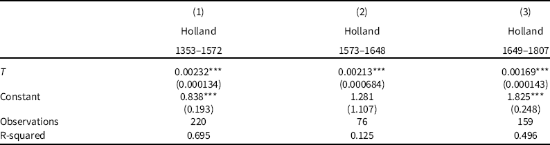
Taking this as our starting point, the next question is what can we learn about the patterns of growth in the pre-industrial economy? To address the same question, De Pleijt and Van Zanden ran a series of regressions to estimate trend growth in the European economy in the period before 1820. Here we summarize the results for the whole period 1270–1822 in Table 1, and for sub-periods in Tables 2 and 3.Footnote ⁴ T in all tables is the estimated trend rate of growth.

Table 1.

Economic growth in England/Britain and Holland, entire period, 1270–1822

Notes: Robust standard errors in parentheses; *** p < 0.01, ** p < 0.05, * p < 0.1.

Table 2.

Economic growth in England and Britain, 1270–1822

Notes: Robust standard errors in parentheses; *** p < 0.01, ** p < 0.05, * p < 0.1.

Table 3.

Economic growth in Holland, 1348–1807

Notes: Robust standard errors in parentheses; *** p < 0.01, ** p < 0.05, * p < 0.1.

All regressions show positive growth rates for the period as a whole and for sub-periods, and there are no indications that there were long periods in which GDP per capita declined, as it is supposed according to Goldstone’s efflorescence hypothesis. This hypothesis of a cyclical growth path therefore has to be rejected.

Are all historical GDP estimates equally good (or bad)?

What we do when we compare levels of GDP per capita in the period before 1850 is to link long-time series of estimates of GDP per capita from different countries with a benchmark estimate of a more or less reliable approximation of the relative levels of GDP per capita in 1820 or 1840 or 1870. The underlying assumption is that all historical series are more or less equally good – or bad – and that therefore errors in all series are of a comparable size, making it possible to assume that they do not matter or do not systematically distort the picture. Here we would like to challenge this idea and focus on systematic differences between groups of historical GDP estimates, which probably produce systematic biases in the estimates involved. In a recent review of the new Broadberry et al. estimates of Chinese GDP in the period 980–1850, Peter Solar produced the following Table 4.Footnote ⁵ It shows that almost 75% of estimated GDP in the base year 1840 was based on grain output. The grain output series therefore completely dominated the movement of GDP. The second most important series is population, which was supposed to ‘represent’ textile, other manufacturing, building, housing and part of commerce (and is somewhat problematic in itself). Other series, such as salt, iron and copper, had only a tiny weight in final GDP.

Table 4.

Weights of underlying series in the GDP estimates, 1840

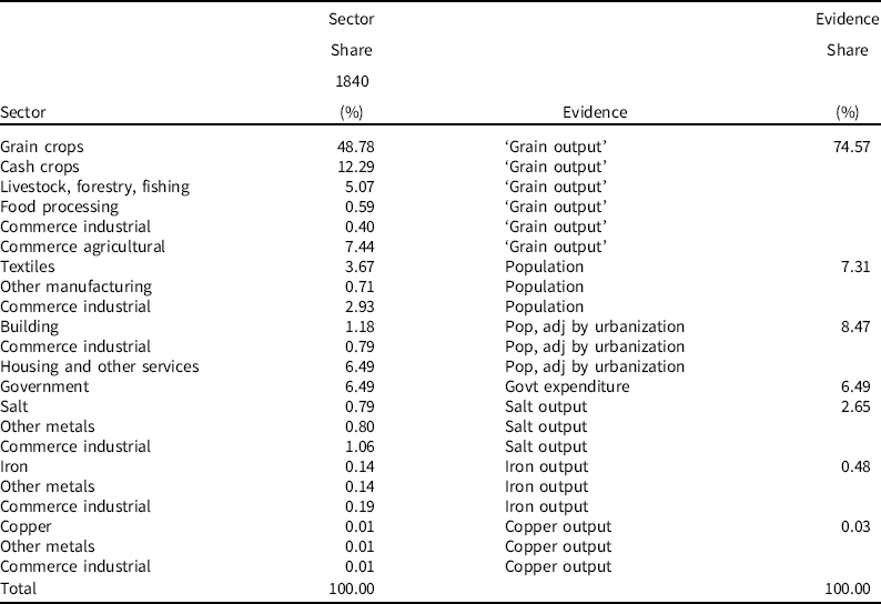
Source: Broadberry, Guan and Li (2018) as summarized by Solar (2020).

This shows, in our view, three problems. The amount of independent, historical information contained in these series is rather limited, compared with contemporary GDP estimates which are based on many hundreds of data sources and time series. This information is weighted very unequally; the series is entirely dominated by one industry – grain farming – which is perhaps least likely to be dynamic, and new and growing activities, such as silk, tea, printing, shipping and many others (in particular, important during the nineteenth century) are not represented at all. The underlying model of the economy is static as the same weighting scheme is used for the entire 980–1850 period, and it is perhaps not unexpected that growth in the long run is low or even negative. GDP per capita declines by 40% between 1020 and 1850. The other new estimates for Chinese GDP in the Qing period by Xu et al. are based on more historical series and a more balanced weighting scheme, but they cover a much shorter period.Footnote ⁶ There is probably a trade-off between the length of the period covered and the amount of data that can be used.

These problems are not limited to the estimates for China. Most pre-1800 estimates for European and Latin American countries are based on an indirect approach, which estimates the demand for foodstuffs on the basis of a ‘standard’ demand function and estimates of the development of real wages. This approach basically combines time series of real wages (based on series of nominal wages and a price index) and the urbanization ratio to get an approximation of GDP per capita. The number of independent time series containing historical information is limited (3–5), the underlying model of the economy is static (the demand function is not changing) and no new products and industries are taken on board. The result is probably that this approach leads to a serious underestimate of long-term economic growth is.

A relatively small group of series, however, in particular those for England 1250–1870 and Holland 1500–1807 (and Indonesia and the Cape Colony), are based on a much larger range of sources and historical time series reflecting the output of almost all important branches of the economy. These output-based estimates do include new activities and products, and the underlying model of the economy is not static but adapted to the changing structure of the economy (weighting schemes, e.g., change over time). These series show, not surprisingly, much more growth than the estimates of the first group. Because Nuvolari and Ricci simulated the indirect model also for the English economy, we can compare how large the difference between the two approaches are.Footnote ⁷ Over the entire 1250–1820 period, the indirect approach (Nuvolari and Ricci) estimates an increase of GDP per capita of 50% (from 84 to 128, at 1700 = 100), whereas according to the direct output approach by Broadberry et al. GDP per capita increased by 150% in the same period.Footnote ⁸ This difference is very large. This might be because England is a particularly dynamic economy undergoing dramatic structural change, but it confirms the intuition that the estimates based on agricultural output (either directly, as in China, or indirectly, as in the case of Italy), and based on only a small number of historical time series, will tend to underestimate growth in the long run. However, Xu et al. found for China between 1738 and 1850 a rather close correlation between the estimates according to the indirect approach (based on real wages in Beijing) and their output-based estimates.Footnote ⁹

These conclusions have important implications for the debate about the question when North-western Europe overtook China, or when England and Holland overtook Italy. If the growth of Chinese GDP per capita is underestimated (or the decline overestimated), this means that the level of Chinese GDP per capita before 1800 will be biased upward (because we start from a benchmark comparison in the nineteenth century). For Italy, there is some direct evidence that this might be correct: the independent benchmark estimates that were made for 1427, comparing Tuscany with England and Holland, showed a much lower relative income level for Tuscany than could be derived from the backward projection of the various time series.Footnote ¹⁰ This suggests, indeed, that Italian economic growth between 1427 and 1820 (or 1860) is underestimated by the Malanima series.Footnote ¹¹ Between, the relative positions of Holland versus England in 1427 (and again in 1562, when a comparison with Poland was made) were more or less consistent with the back-projections based on the two times series of GDP per capita.

Summing up, given these biases in the series for China and Italy (and Spain, Germany and France) the current estimates for these countries probably tend to overstate GDP per capita before 1820 (and to underestimate growth), and therefore tend to date the moment at which the lines cross too late. Only by reconstructing new benchmarks for the pre-1820 period (or by making more broadly based output estimates comparable with those for England and Holland) can we really get a more detailed timing of the convergence and divergence of those economies in the pre-1800 period.

What can be done to be more transparent about these differences in the quality of the estimated series? We suggest that the ‘Solar-table’ should be included in new papers presenting time series of historical national accounts. Authors should be more explicit about the number of historical time series that form the basis of their estimates, and the way in which these are weighted. Often this information is included in the paper, but not presented in this systematic way. We also suggest that the current practice of discussing margins of error is slightly misleading. It focuses only on the margins of error of the underlying series (how good is the population series for China?), but does not take into account the fact that often series are used as substitute for the ‘real’ data (what are the implications of assuming that a population series is used as a proxy for the output of textiles?) By narrowing the discussion of margins or error down to the question how reliable these series are for what they stand for (how large are the margins of error of the population series?) a large part of the true uncertainty is ignored.