


1. Introduction
The damping rate of the interface of a viscoelastic liquid, such as a polymeric solution, depends on both its viscous and elastic properties, when the fluid is subjected to momentary disturbances. The viscous component dissipates the imposed disturbances, while the elastic component gives rise to restorative forces due to elastic stresses. The memory associated with these stresses therefore alters the behaviour of the fluid when it is subjected to time-periodic acceleration, which is the subject of the current study.
The influence of viscoelasticity is apparent in its notable impact on the instability threshold that arises from parametric forcing, as reported in early theoretical studies (Kumar Reference Kumar1999; Müller & Zimmermann Reference Müller and Zimmermann1999). These theoretical investigations compared the resonant characteristics of Newtonian fluids with polymeric solutions in the presence of gravity. The onset of the instability, known as Faraday instability, was predicted by a mathematical model similar to the one proposed by Kumar & Tuckerman (Reference Kumar and Tuckerman1994), upon incorporating a Maxwell constitutive relationship (Bird et al. Reference Bird, Armstrong and Hassager1987). The mechanical analogue of the dynamic behaviour of Maxwell fluids is often represented by a dashpot and spring in series, where the dashpot reflects the viscous response to disturbances and the spring reflects the elastic response (Guyon et al. Reference Guyon, Hulin, Petit and Mitescu2015). Viscoelastic fluids, such as the one studied by Kumar (Reference Kumar1999) and Müller & Zimmermann (Reference Müller and Zimmermann1999), following a Maxwell constitutive relationship, behave more like a viscous liquid under low-frequency oscillatory disturbances and more like an elastic solid under high-frequency oscillatory disturbances. By contrast, soft polymeric gels characterized by Kelvin–Voigt constitutive laws exhibit the opposite response (Morozov & Spagnolie Reference Morozov and Spagnolie2015). Likewise, different dynamic behaviour and temporal response are reported when solid gels are subjected to parametric forcing as seen in several interesting studies (Shao et al. Reference Shao, Saylor and Bostwick2018, Reference Shao, Bevilacqua, Ciarletta, Saylor and Bostwick2020; Bevilacqua et al. Reference Bevilacqua, Shao, Saylor, Bostwick and Ciarletta2020).
Focusing on the dynamical behaviour of a Maxwell fluid in the presence of parametric forcing, linear stability calculations were performed by Kumar (Reference Kumar1999) and Müller & Zimmermann (Reference Müller and Zimmermann1999) who assumed the properties of various polymer solutions with different levels of elasticity, expressed in terms of the relaxation time, i.e. the time scale for the polymer chains to relax within the solvent. It was demonstrated that the threshold amplitude for the onset of Faraday instability decreases with an increase in elasticity. The findings of these studies, which assumed infinitely wide and deep fluid layers, revealed a predominantly harmonic interface response for frequency ranges where the forcing frequency is close to the inverse of the relaxation time. Beyond these frequency ranges, it was shown that a subharmonic mode becomes more unstable than the harmonic mode. This is in contrast to a Newtonian liquid, where a subharmonic response is always dominant in deep liquid layers (Kumar Reference Kumar1996). In the work of Kumar (Reference Kumar1999), Faraday forcing in finite depths were also considered and it was observed that the harmonic mode becomes more dominant than the case of infinitely deep liquids. This result was attributed to increased vertical viscous stresses.
Experimental validation of these theories was provided by Wagner et al. (Reference Wagner, Müller and Knorr1999) who used a dilute solution of polyacrylamide-co-acrylic acid polymer in a glycerol–water mixture solvent. Such a fluid mixture is not shear-thinning and follows a Maxwell constitutive relation. Through these experiments, the authors not only confirmed the presence of harmonic patterns but also demonstrated that the theoretical models of Müller & Zimmermann (Reference Müller and Zimmermann1999) and Kumar (Reference Kumar1999) accurately predict the experimental onset of Faraday waves. By contrast, experiments performed by Raynal et al. (Reference Raynal, Kumar and Fauve1999), Ballesta & Manneville (Reference Ballesta and Manneville2005) and Cabeza & Rosen (Reference Cabeza and Rosen2007) employing shear-thinning polymeric solutions, while showing qualitative agreement, revealed quantitative discrepancies with the theories for non-shear-thinning fluids (Kumar Reference Kumar1999; Müller & Zimmermann Reference Müller and Zimmermann1999).
In a recent study, Schön & Bestehorn (Reference Schön and Bestehorn2023) investigated the threshold limits and nonlinear behaviour of the interface of a Maxwell fluid undergoing resonant instability. They used a reduced-order model, making a thin-layer approximation that included both inertial and elastic terms, crucial to predicting the Faraday instability. Using this model, they observed that the threshold amplitude for the onset of Faraday instability decreases with an increase in frequency and does so at a faster rate compared with a Newtonian liquid.
The principal purpose of the current work is to study the effect of different gravity levels on the parametric forcing of a layer of viscoelastic fluid. To this end, we consider the same constitutive model, i.e. the Maxwell model, studied theoretically by Kumar (Reference Kumar1999), Müller & Zimmermann (Reference Müller and Zimmermann1999), Schön & Bestehorn (Reference Schön and Bestehorn2023) and experimentally by Wagner et al. (Reference Wagner, Müller and Knorr1999), now focusing on the effect of gravity on a parametrically forced viscoelastic fluid layer.
The current work differs from earlier studies on gravitationally stable configurations in two significant ways. First, we present new findings for the gravitationally stable case in the weakly elastic limit. Second, we examine two additional scenarios: one in which gravity is weak, i.e. the microgravity case and another where the system becomes gravitationally unstable. As a result, we make several important observations. In the gravitationally stable case, while Kumar (Reference Kumar1999) observed that the threshold for Faraday instability decreases as the Deborah number increases for high Deborah values under Earth’s gravity, our study goes further by exploring weakly elastic fluids, i.e. having small relaxation times. Upon doing so, we find that in the weakly elastic limit, the threshold for Faraday instability actually increases with elasticity, which contrasts with the behaviour observed in strongly elastic fluids. These results are supported by asymptotic expressions for the inverse time constants in the long-wavelength limit. In the microgravity case, we observe a striking transition from oscillatory to monotonic behaviour as the gravity level decreases. As gravity approaches zero, monotonic instability dominates, a phenomenon that has not been previously reported. This shift to monotonic instability in microgravity has implications for the case in which the fluid is gravitationally unstable. Finally, in the gravitationally unstable case, unlike the case of Newtonian fluids where parametric forcing always has a stabilizing effect (Sterman-Cohen et al. Reference Sterman-Cohen, Bestehorn and Oron2017), the present study reveals the possibility of either stabilization or destabilization for the case of viscoelastic fluids. Specifically, upon considering fluids of finite lateral extent, we find a range of forcing amplitudes between two critical parametric frequencies where we can stabilize an otherwise gravitationally unstable system, without triggering resonance. This stands in stark contrast to a Newtonian fluid system where we have only one critical frequency below which complete stabilization may be achieved (Ignatius et al. Reference Ignatius, Dinesh, Dietze and Narayanan2024). These new results are supported by algebraic expressions derived from a low-dimensional model based on a long-wavelength approximation (Ruyer-Quil & Manneville Reference Ruyer-Quil and Manneville2000). These expressions not only predict the instability ranges but also provide insight into the physical phenomena involved in the parametric forcing of viscoelastic fluids.
The manuscript is arranged as follows. In § 2, we give the mathematical model for the parametric forcing of a Maxwell liquid in a configuration as described in figure 1. In § 3, we investigate the effect of elasticity on the fluid’s damping rates, or more generally the inverse time constants, to momentary disturbances. The behaviour of the inverse time constants with fluid elasticity forecasts the effect of the latter on the threshold amplitude of Faraday instability as well as the interface’s temporal response in both gravitationally stable and microgravity configurations. This is analysed in § 4. Finally, in § 5, we discuss the influence of parametric forcing on a gravitationally unstable viscoelastic system.
2. Mathematical model
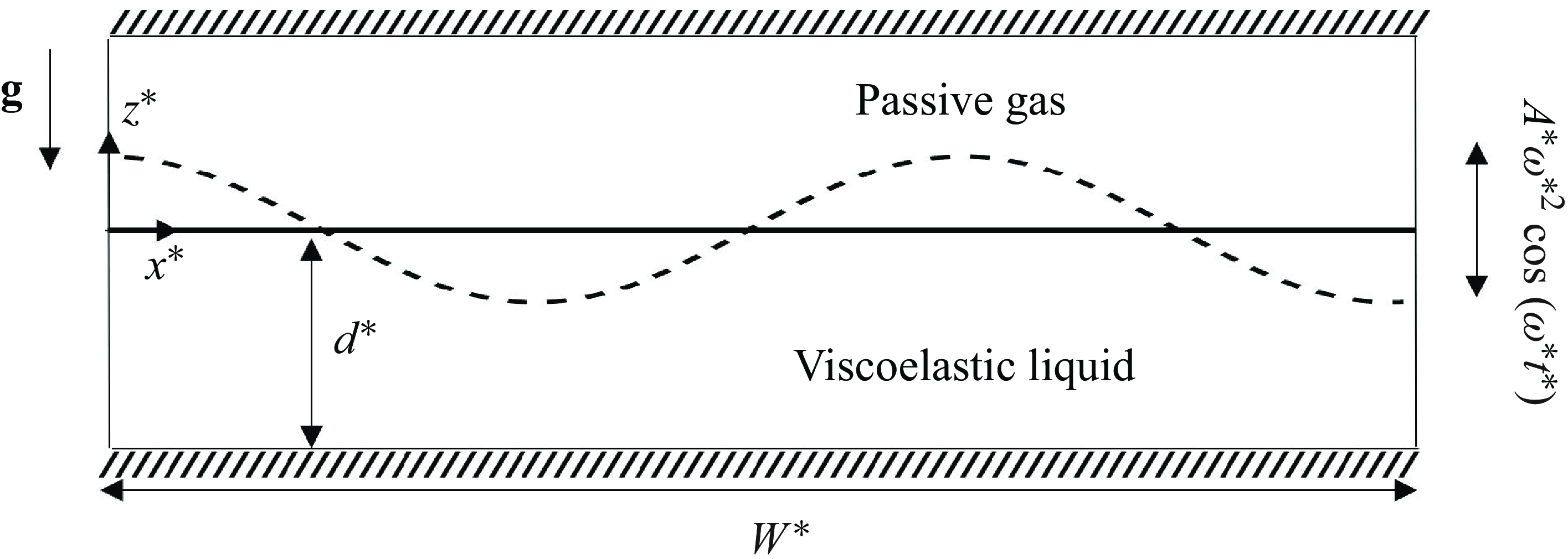
Consider a viscoelastic liquid layer of unperturbed height, $d^*$
, in a container of width,
$d^*$
, in a container of width, $W^{*}$
, and in contact with a passive gas as shown in figure 1. The fluid system is subjected to the gravitational acceleration,
$W^{*}$
, and in contact with a passive gas as shown in figure 1. The fluid system is subjected to the gravitational acceleration, $\mathbf{g}$
, and a mechanical oscillation of angular frequency,
$\mathbf{g}$
, and a mechanical oscillation of angular frequency, $\omega ^*$
, and amplitude,
$\omega ^*$
, and amplitude, $A^*$
, in the direction of gravity. We consider this system in the moving frame of reference,
$A^*$
, in the direction of gravity. We consider this system in the moving frame of reference, $x^*$
,
$x^*$
, $z^*$
, i.e. a frame that rests on the initial flat interface and moving with the container. In addition to properties such as density,
$z^*$
, i.e. a frame that rests on the initial flat interface and moving with the container. In addition to properties such as density, $\rho$
, viscosity,
$\rho$
, viscosity, $\mu$
, and surface tension,
$\mu$
, and surface tension, $\gamma$
, the liquid possesses a shear modulus,
$\gamma$
, the liquid possesses a shear modulus, $G$
, which imparts elastic character. Fluid flow in the system is governed by the nonlinear equations of momentum subject to continuity and appropriate interfacial conditions. These are expressed next in the moving frame of reference first in unscaled form, and then rendered dimensionless using suitable scaling variables.
$G$
, which imparts elastic character. Fluid flow in the system is governed by the nonlinear equations of momentum subject to continuity and appropriate interfacial conditions. These are expressed next in the moving frame of reference first in unscaled form, and then rendered dimensionless using suitable scaling variables.
Schematic of the studied configuration in the moving frame of reference. Depicted is a viscoelastic liquid layer in contact with a passive gas aligned with the gravity vector, $\mathbf{g}$
. The fluid container is subject to a vertical mechanical acceleration,
$\mathbf{g}$
. The fluid container is subject to a vertical mechanical acceleration, $A^*\omega {^*}^2 \cos(\omega ^* t^*)\mathbf{e}_{\mathbf{\textit{z}}}$
, with respect to the laboratory frame.
$A^*\omega {^*}^2 \cos(\omega ^* t^*)\mathbf{e}_{\mathbf{\textit{z}}}$
, with respect to the laboratory frame.
2.1. Nonlinear equations
The continuity and momentum equations are
 \begin{equation} {\boldsymbol{\nabla}^*.\mathbf{v}^*} =0 \end{equation}
and
 \begin{equation} \rho \left (\frac {\partial {\mathbf{v}^*}}{\partial t^*}+{\mathbf{v}^*}\cdot {\boldsymbol{\nabla}}^* {\mathbf{v}^* }\right ) = -{\boldsymbol{\nabla}}^*p^*+ {\boldsymbol{\nabla}}^* \cdot \boldsymbol {\tau} ^* - \rho \Bigl (g + A^*\omega {^*}^2 cos(\omega ^* t^*)\Bigr )\mathbf{e}_{\mathbf{\textit{z}}}, \end{equation}
where $\boldsymbol {\tau }^*$
is the stress tensor and
$\boldsymbol {\tau }^*$
is the stress tensor and $\mathbf{e}_{\mathbf{\textit{z}}}$
is the unit vector in the
$\mathbf{e}_{\mathbf{\textit{z}}}$
is the unit vector in the $z$
-direction. The constitutive equation for the viscoelastic liquid is described by an upper-convected Maxwell equation (Morozov & Spagnolie Reference Morozov and Spagnolie2015), a nonlinear model that includes frame-invariant derivatives in the stress-strain rate relationship. This is expressed as
$z$
-direction. The constitutive equation for the viscoelastic liquid is described by an upper-convected Maxwell equation (Morozov & Spagnolie Reference Morozov and Spagnolie2015), a nonlinear model that includes frame-invariant derivatives in the stress-strain rate relationship. This is expressed as
 \begin{equation} \boldsymbol {\tau }^*+\lambda \left (\frac {\partial \boldsymbol {\tau }^*}{\partial t^*}+{\mathbf{v}^*}\cdot {\boldsymbol{\nabla}}^* \boldsymbol {\tau} ^* -(\boldsymbol{\nabla}^* {\mathbf{v}^*})^T\cdot \boldsymbol {\tau }^*-\boldsymbol {\tau }^*\cdot (\boldsymbol{\nabla}^* {\mathbf{v}^*})\right )=\mu \Bigl ({\boldsymbol{\nabla}^* \mathbf{v}^*}+({\boldsymbol{\nabla}^* \mathbf{v}^*})^T\Bigr ), \end{equation}
where $\lambda ={\mu}/{G}$
is the relaxation time.
$\lambda ={\mu}/{G}$
is the relaxation time.
At the bottom wall, $z^*$
=
$z^*$
= $-d^*$
, we impose no-slip and no-penetration conditions, i.e.
$-d^*$
, we impose no-slip and no-penetration conditions, i.e.
 \begin{equation} {\mathbf{v}^*}=\mathbf{0}. \end{equation}
At the impenetrable interface, $z^*=h^*({\mathbf{x}^*},t^*)$
, the jump mass balance gives
$z^*=h^*({\mathbf{x}^*},t^*)$
, the jump mass balance gives
 \begin{equation} ({\mathbf{v}^*}- {\mathbf{u}^*})\cdot {\mathbf{n}^*}=0. \end{equation}
The jump force balance yields an equation in terms of the stress tensor, $\boldsymbol {\tau} ^*$
, and is given by
$\boldsymbol {\tau} ^*$
, and is given by
 \begin{equation} -p^*{\mathbf{n}^*}+{\mathbf{n}^*}\cdot {\boldsymbol {\tau} ^*}+\gamma \,{\mathbf{n}^*}\boldsymbol{\nabla}^*\cdot {\mathbf{n}^*}=0, \end{equation}
for which the interface speed, ${\mathbf{u}^*}\cdot {\mathbf{n}^*}$
, and the unit normal,
${\mathbf{u}^*}\cdot {\mathbf{n}^*}$
, and the unit normal, ${\mathbf{n}^*}$
, are given by
${\mathbf{n}^*}$
, are given by
 \begin{equation} {\mathbf{u}^*}\cdot {\mathbf{n}^*}=\cfrac {\cfrac {\partial h^*}{\partial t^*}}{\left (1+\left (\cfrac {\partial h^*}{\partial x^*}\right )^{2} \right )^{\frac {1}{2}}}\,\,\text{and}\,\,{\mathbf{n}^*}= \cfrac {-\cfrac {\partial h^*}{\partial x^*}\, {\mathbf{e}_{\mathbf{\textit{x}}}} +\mathbf{e}_{\mathbf{\textit{z}}}}{\left (1+\left (\cfrac {\partial h^*}{\partial x^*}\right )^2 \right )^{\frac {1}{2}}}. \end{equation}
The characteristic scales used to convert the governing equations into scaled form are
 \begin{equation} \begin{aligned} x=\frac {x^*}{W^*},\,\, z=\frac {z^*}{d^*}, \,\, t= \frac {t^*}{\Bigl (\cfrac {d^*}{\epsilon U}\Bigr )},\,\, \omega =\omega ^*\,\,\Bigl (\frac {d^*}{\epsilon U}\Bigr ), \,\, u=\frac {u^*}{U}, \,\, w=\frac {w^*}{\epsilon U},\\ \,\,p= \frac {p^*}{\Bigl (\cfrac {\mu U}{d^*}\Bigr )},\,\tau _{xx}= \frac {\tau ^*_{xx}}{\Bigl (\cfrac {\epsilon \mu U}{d^*}\Bigr )},\,\,\,\tau _{xz}= \frac {\tau ^*_{xz}}{\Bigl (\cfrac {\mu U}{d^*}\Bigr )}\,\mbox{and}\,\, \,\tau _{zz}= \frac {\tau ^*_{zz}}{\Bigl (\cfrac {\epsilon \mu U}{d^*}\Bigr )}, \end{aligned} \end{equation}
where $U$
is a characteristic velocity in the
$U$
is a characteristic velocity in the $x$
-direction to be defined in § 4, (4.1).
$x$
-direction to be defined in § 4, (4.1).
Note that we render $x$
and
$x$
and $z$
dimensionless using
$z$
dimensionless using $W^*$
and
$W^*$
and $d^*$
, respectively. This leads to a length scale separation parameter,
$d^*$
, respectively. This leads to a length scale separation parameter, $\epsilon$
, given by
$\epsilon$
, given by $\epsilon =d^*/W^*$
, which will play an important role when we consider the long-wave limit of the problem to derive algebraic formulae that can predict stability ranges. Non-dimensionalizing equations (2.1) and (2.2) and expressing them in component form, we get
$\epsilon =d^*/W^*$
, which will play an important role when we consider the long-wave limit of the problem to derive algebraic formulae that can predict stability ranges. Non-dimensionalizing equations (2.1) and (2.2) and expressing them in component form, we get
 \begin{equation} \frac {\partial u}{\partial x}+\frac {\partial w}{\partial z}=0, \end{equation}
 \begin{equation} \epsilon Re \left (\frac {\partial u}{\partial t}+u\frac {\partial u}{\partial x}+w\frac {\partial u}{\partial z} \right ) = -\epsilon \frac {\partial p}{\partial x} + \epsilon ^2\frac {\partial \tau _{xx}}{\partial x} +\frac {\partial \tau _{xz}}{\partial z} \end{equation}
and
 \begin{equation} \epsilon ^3 Re \left (\frac {\partial w}{\partial t}+u\frac {\partial w}{\partial x}+w\frac {\partial w}{\partial z} \right )= -\epsilon \frac {\partial p}{\partial z} + \epsilon ^2\frac {\partial \tau _{xz}}{\partial x}+\epsilon ^2\frac {\partial \tau _{zz}}{\partial z} - \,\epsilon (\mathcal{G} +\mathcal{A} \cos(\omega t)). \end{equation}
Likewise the scaling of (2.3) yields
 \begin{equation} \tau _{xx}+ De\left [\frac {\partial \tau _{xx}}{\partial t}+u\frac {\partial \tau _{xx}}{\partial x}+w\frac {\partial \tau _{xx}}{\partial z}-2 \left (\tau _{xx}\frac {\partial u}{\partial x}+\frac {1}{\epsilon ^2}\tau _{xz}\frac {\partial u}{\partial z}\right )\,\,\right ]=2 \frac {\partial u}{\partial x}, \end{equation}
 \begin{equation} \tau _{xz}+ De\left [\frac {\partial \tau _{xz}}{\partial t}+u\frac {\partial \tau _{xz}}{\partial x}+w\frac {\partial \tau _{xz}}{\partial z}- \left (\epsilon ^2 \tau _{xx}\frac {\partial w}{\partial x}+\tau _{zz}\frac {\partial u}{\partial z}\right )\,\,\right ]= \frac {\partial u}{\partial z}+\epsilon ^2\frac {\partial w}{\partial x} \end{equation}
and
 \begin{equation} \, \tau _{zz}+ De\left [\frac {\partial \tau _{zz}}{\partial t}+u\frac {\partial \tau _{zz}}{\partial x}+w\frac {\partial \tau _{zz}}{\partial z}-2 \left (\tau _{xz} \frac {\partial w}{\partial x}+\tau _{zz}\frac {\partial w}{\partial z}\right )\,\,\right ]=2 \frac {\partial w}{\partial z}. \end{equation}
In the above, the Reynolds number is given by $Re={\rho U d^*}/{\mu }$
. It is the ratio of the characteristic time due to viscous damping and the characteristic time due to flow. The Deborah number,
$Re={\rho U d^*}/{\mu }$
. It is the ratio of the characteristic time due to viscous damping and the characteristic time due to flow. The Deborah number, $De=\lambda ({\epsilon U}/{d^*})=({\mu }/{G })({\epsilon U}/{d^*})$
characterizes the ratio of the relaxation time due to elasticity and the characteristic time due to flow. The ratio
$De=\lambda ({\epsilon U}/{d^*})=({\mu }/{G })({\epsilon U}/{d^*})$
characterizes the ratio of the relaxation time due to elasticity and the characteristic time due to flow. The ratio $De/Re$
is thus independent of the characteristic flow speed,
$De/Re$
is thus independent of the characteristic flow speed, $U$
. The scaled gravity is given by
$U$
. The scaled gravity is given by $\mathcal{G}={\rho g d{^*}^{2}}/({\mu U)}$
and scaled forcing amplitude becomes
$\mathcal{G}={\rho g d{^*}^{2}}/({\mu U)}$
and scaled forcing amplitude becomes $\mathcal{A}$
=
$\mathcal{A}$
= ${\rho A^* \omega {^*}^{2}d{^*}^{2}}/({\mu U)}$
.
${\rho A^* \omega {^*}^{2}d{^*}^{2}}/({\mu U)}$
.
The scaled boundary conditions are
 \begin{equation} u=0\,\,\text{and}\,\, w=0\,\,\mbox{at}\,\, z=-1, \end{equation}
while at the interface, $z=h(x,t)$
, the jump mass balance condition become
$z=h(x,t)$
, the jump mass balance condition become
 \begin{equation} \epsilon w-\epsilon u \frac {\partial h}{\partial x} =\epsilon \frac {\partial h}{\partial t}, \end{equation}
and the tangential and normal components of the force balance become
 \begin{equation} \,\,\tau _{xz}\left (1-\epsilon ^2 \left (\frac {\partial h}{\partial x}\right )^2\right )+ \epsilon ^2 (\tau _{zz}-\tau _{xx})\frac {\partial h}{\partial x}=0 \end{equation}
and
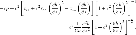 \begin{equation} \begin{aligned} \,\,-\epsilon p+\epsilon ^2\left [ \tau _{zz}+\epsilon ^2 \tau _{xx}\left (\frac {\partial h}{\partial x}\right )^2-\tau _{xz}\left (\frac {\partial h}{\partial x}\right )\right ]\left [ 1+\epsilon ^2\left (\frac {\partial h}{\partial x}\right )^{2}\right ]^{-1}\\= \epsilon ^3 \frac {1}{Ca} \frac {\partial ^2 h}{\partial x^{2}}\left [ 1+\epsilon ^2\left (\frac {\partial h}{\partial x}\right )^{2}\right ]^{-\frac {3}{2}}, \end{aligned} \end{equation}
where $Ca={\mu U}/ {\gamma }$
is the capillary number.
$Ca={\mu U}/ {\gamma }$
is the capillary number.
In nonlinear simulations, solving (2.11) at high $De$
can lead to numerical instabilities. Methods to address such issues in viscoelastic flow have been reviewed by Alves et al. (Reference Alves, Oliveira and Pinho2021). For instance, Sureshkumar & Beris (Reference Sureshkumar and Beris1995) introduced an artificial diffusive stress term to suppress instabilities, which necessitates specifying boundary conditions for the stress tensor. In our study, however, we do not perform nonlinear simulations and thus do not encounter numerical instabilities. Instead, we use linear stability analysis where, as we shall see in § 2.2, the stress tensor components can be directly determined in terms of velocity components or their spatial derivatives (see (2.19)).
$De$
can lead to numerical instabilities. Methods to address such issues in viscoelastic flow have been reviewed by Alves et al. (Reference Alves, Oliveira and Pinho2021). For instance, Sureshkumar & Beris (Reference Sureshkumar and Beris1995) introduced an artificial diffusive stress term to suppress instabilities, which necessitates specifying boundary conditions for the stress tensor. In our study, however, we do not perform nonlinear simulations and thus do not encounter numerical instabilities. Instead, we use linear stability analysis where, as we shall see in § 2.2, the stress tensor components can be directly determined in terms of velocity components or their spatial derivatives (see (2.19)).
2.2. Linear stability
Assuming stress-free side conditions at $x=0$
and
$x=0$
and $x=1$
, the governing equations (2.9)–(2.13) are perturbed around the base state, which is quiescent with respect to the moving frame of reference, using
$x=1$
, the governing equations (2.9)–(2.13) are perturbed around the base state, which is quiescent with respect to the moving frame of reference, using
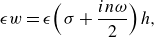
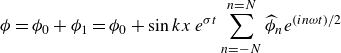 \begin{equation} \phi =\phi _{0}+\phi _{1}=\phi _{0}+ \sin {kx}\,e^{\sigma t}\sum _{n=-N}^{n=N}\widehat {\phi }_n e^{(in\omega t)/2} \end{equation}
and
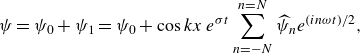 \begin{equation} \psi =\psi _{0}+\psi _{1}=\psi _{0}+ \cos {kx}\,e^{\sigma t}\sum _{n=-N}^{n=N}\widehat {\psi }_n e^{(in\omega t)/2}, \end{equation}
where $\phi$
corresponds to the unknown dependent variables
$\phi$
corresponds to the unknown dependent variables $u$
and
$u$
and $\tau _{xz}$
and
$\tau _{xz}$
and $\psi$
corresponds to
$\psi$
corresponds to $w$
,
$w$
, $\tau _{xx}$
,
$\tau _{xx}$
, $\tau _{zz}$
,
$\tau _{zz}$
, $p$
and
$p$
and $h$
. The subscript
$h$
. The subscript $1$
denotes the infinitesimal disturbance with a wavenumber,
$1$
denotes the infinitesimal disturbance with a wavenumber, $k$
, and an inverse time constant,
$k$
, and an inverse time constant, $\sigma$
. The summation in (2.14) and (2.15) ensures compatibility with the parametric forcing term in (2.10b
), with
$\sigma$
. The summation in (2.14) and (2.15) ensures compatibility with the parametric forcing term in (2.10b
), with $N$
denoting the number of oscillatory modes considered (Nayfeh Reference Nayfeh1981). The quiescent base state (denoted by subscript 0) is given by
$N$
denoting the number of oscillatory modes considered (Nayfeh Reference Nayfeh1981). The quiescent base state (denoted by subscript 0) is given by
 \begin{equation} u_0=w_0=0, \,\tau _{xx0}=\tau _{xz0}=\tau _{zz0}=0, \, -\frac {\partial p_0}{\partial z}=\mathcal{G}+\mathcal{A} cos(\omega t)\,\mbox{and} \, \,h_0=0. \end{equation}
Next, we substitute the forms given by (2.14), (2.15) and (2.16), into (2.9)–(2.13) and linearize these in terms of the amplitudes $\widehat {\phi }$
and
$\widehat {\phi }$
and $\widehat {\psi }$
. In the resulting equations, (2.17)–(2.23), which are written below, we have dropped for convenience the terminology related to the summation over the temporal modes, except for (2.23). Thus, we obtain
$\widehat {\psi }$
. In the resulting equations, (2.17)–(2.23), which are written below, we have dropped for convenience the terminology related to the summation over the temporal modes, except for (2.23). Thus, we obtain
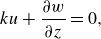 \begin{equation} k u+\frac {\partial w}{\partial z}=0, \end{equation}
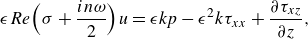 \begin{equation} \epsilon Re \Bigl (\sigma + \frac {i n \omega }{2}\Bigr ) u = \epsilon k p - \epsilon ^2 k \tau _{xx} +\frac {\partial \tau _{xz}}{\partial z}, \end{equation}
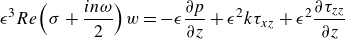 \begin{equation} \epsilon ^3 Re \Bigl (\sigma + \frac {i n \omega }{2}\Bigr ) w= -\epsilon \frac {\partial p}{\partial z} + \epsilon ^2 k\tau _{xz}+\epsilon ^2\frac {\partial \tau _{zz}}{\partial z} \end{equation}
and
 \begin{equation} \begin{aligned} \tau _{xx}+ De \Bigl (\sigma + \frac {i n \omega }{2}\Bigr ) \tau _{xx}=2 k u,\,\,\tau _{xz}+ De\Bigl (\sigma + \frac {i n \omega }{2}\Bigr ) \tau _{xz}= \frac {\partial u}{\partial z}-\epsilon ^2 k w \\ \,\mbox{and}\,\,\,\,\,\,\,\,\,\,\,\,\,\,\,\,\,\,\, \tau _{zz}+ De\Bigl (\sigma + \frac {i n \omega }{2}\Bigr ) \tau _{zz}=2 \frac {\partial w}{\partial z}.\,\,\,\,\,\,\,\,\,\,\,\,\,\,\,\, \end{aligned} \end{equation}
Equations (2.19) reflect the same constitutive relationship used by Müller & Zimmermann (Reference Müller and Zimmermann1999), Kumar (Reference Kumar1999) and Schön & Bestehorn (Reference Schön and Bestehorn2023). At the bottom wall, $z=-1$
, we have
$z=-1$
, we have
 \begin{equation} u=0\,\,\mbox{and}\, \,w=0 \end{equation}
and at the interface, $z=0$
, we have
$z=0$
, we have
 \begin{equation} \epsilon w= \epsilon \Bigl (\sigma + \frac {i n \omega }{2}\Bigr ) h, \end{equation}
 \begin{equation} \tau _{xz} =0 \end{equation}
and
 \begin{equation} \sum _{n=-N}^{n=N} e^{(in\omega t)/2} \Bigl \{- \epsilon \widehat {p}_n + \epsilon [\mathcal{G} +\mathcal{A}\,cos(\omega t)]\widehat {h}_n+ \epsilon ^2 \widehat {\tau }_{zz\,n}+k^2 \epsilon ^3 \frac {1}{Ca}\widehat {h}_n\Bigr \}=0. \end{equation}
The above linearized equations are examined from two perspectives. In the first perspective, $\mathcal{A}$
and
$\mathcal{A}$
and $\omega$
are set to zero and the set of the inverse time constants,
$\omega$
are set to zero and the set of the inverse time constants, $\sigma$
, is then computed, observing that, in general,
$\sigma$
, is then computed, observing that, in general, $\sigma$
is complex. The real parts of
$\sigma$
is complex. The real parts of $\sigma$
are negative when the fluid is in a gravitationally stable configuration. The leading
$\sigma$
are negative when the fluid is in a gravitationally stable configuration. The leading $\sigma$
is the inverse time constant whose real part is the least negative among all complex
$\sigma$
is the inverse time constant whose real part is the least negative among all complex $\sigma$
. The imaginary part of the leading
$\sigma$
. The imaginary part of the leading $\sigma$
gives an estimate of the natural frequency of the system (Dinesh et al. Reference Dinesh, Livesay, Ignatius and Narayanan2023). When a system is parametrically forced at its natural frequency, resonance-induced instability is known to occur (Kumar & Tuckerman Reference Kumar and Tuckerman1994). Knowing how the real part of the leading
$\sigma$
gives an estimate of the natural frequency of the system (Dinesh et al. Reference Dinesh, Livesay, Ignatius and Narayanan2023). When a system is parametrically forced at its natural frequency, resonance-induced instability is known to occur (Kumar & Tuckerman Reference Kumar and Tuckerman1994). Knowing how the real part of the leading $\sigma$
behaves with
$\sigma$
behaves with $De$
informs us on how the threshold of the instability behaves. The more negative the leading
$De$
informs us on how the threshold of the instability behaves. The more negative the leading $\sigma$
, the higher the threshold of the resonance-induced instability. To obtain analytical expressions on the behaviour of
$\sigma$
, the higher the threshold of the resonance-induced instability. To obtain analytical expressions on the behaviour of $\sigma$
with
$\sigma$
with $De$
we appeal to a reduced-order model (the derivation of which is given in Appendix A).
$De$
we appeal to a reduced-order model (the derivation of which is given in Appendix A).
In the second perspective, the dimensionless forcing amplitude, $\mathcal{A}$
, is calculated by setting
$\mathcal{A}$
, is calculated by setting $\sigma$
to zero and expressing the dependent variables in terms of the interface deflection,
$\sigma$
to zero and expressing the dependent variables in terms of the interface deflection, $h$
(Kumar & Tuckerman Reference Kumar and Tuckerman1994). This results in an eigenvalue problem arising from (2.23) and takes the form
$h$
(Kumar & Tuckerman Reference Kumar and Tuckerman1994). This results in an eigenvalue problem arising from (2.23) and takes the form
 \begin{equation} \mathbf{Cx}=\mathcal{A}\,\mathbf{Dx}, \end{equation}
with eigenvalues, $\mathcal{A}$
, and eigenvectors
$\mathcal{A}$
, and eigenvectors $\mathbf{x}=\{\widehat {h}_N,\widehat {h}_{N-1}\ldots .\widehat {h}_{-N}\}$
. The detailed forms of the matrices,
$\mathbf{x}=\{\widehat {h}_N,\widehat {h}_{N-1}\ldots .\widehat {h}_{-N}\}$
. The detailed forms of the matrices, $\mathbf{C}$
and
$\mathbf{C}$
and $\mathbf{D}$
, are provided in Appendix B. It should be noted that the eigenvalues will appear in pairs as
$\mathbf{D}$
, are provided in Appendix B. It should be noted that the eigenvalues will appear in pairs as $\pm \mathcal{A}$
on account of the periodic forcing term given in (2.2). We therefore take
$\pm \mathcal{A}$
on account of the periodic forcing term given in (2.2). We therefore take $\mathcal{A}$
to be positive without any loss of generality. The solutions to the eigenvalue problem (2.24) are numerically obtained using the Eigenvalue routine in Mathematica®. The neutral stability curves,
$\mathcal{A}$
to be positive without any loss of generality. The solutions to the eigenvalue problem (2.24) are numerically obtained using the Eigenvalue routine in Mathematica®. The neutral stability curves, $\mathcal{A}$
versus
$\mathcal{A}$
versus $k$
, thus obtained are used to examine the effect of viscoelasticity on the resonant or Faraday instability. These calculations are done by relaxing the assumption of small
$k$
, thus obtained are used to examine the effect of viscoelasticity on the resonant or Faraday instability. These calculations are done by relaxing the assumption of small $\epsilon$
, thereby allowing consideration of arbitrary wavenumbers,
$\epsilon$
, thereby allowing consideration of arbitrary wavenumbers, $k$
. This is done by using a common length scale,
$k$
. This is done by using a common length scale, $d^*$
, which amounts to scaling the horizontal direction with
$d^*$
, which amounts to scaling the horizontal direction with $d^*$
and setting
$d^*$
and setting $\epsilon =1$
in the scaled forms given in (2.8).
$\epsilon =1$
in the scaled forms given in (2.8).
The threshold amplitude, numerically obtained using (2.24), can also be obtained accurately for low wavenumbers by appealing to a reduced-order model (assuming $\epsilon \lt \lt 1)$
derived in Appendix A. The advantage of this model is that it provides explicit relations for
$\epsilon \lt \lt 1)$
derived in Appendix A. The advantage of this model is that it provides explicit relations for $\sigma$
and
$\sigma$
and $\mathcal{A}$
as functions of the wavenumber,
$\mathcal{A}$
as functions of the wavenumber, $k$
, without having to determine the eigenfunctions. We now briefly discuss the main results arising from such a model.
$k$
, without having to determine the eigenfunctions. We now briefly discuss the main results arising from such a model.
2.3. A brief discussion on the reduced-order model
The reduced model is obtained upon dropping terms of O( $\epsilon ^2$
) in (2.17) to (2.23) and integrating (2.17) to (2.19) along the z-direction using (2.20) to (2.23) (Kalliadasis et al. Reference Kalliadasis, Ruyer-Quil, Scheid and Velarde2011). The model yields the following dispersion relation (cf. (A20))
$\epsilon ^2$
) in (2.17) to (2.23) and integrating (2.17) to (2.19) along the z-direction using (2.20) to (2.23) (Kalliadasis et al. Reference Kalliadasis, Ruyer-Quil, Scheid and Velarde2011). The model yields the following dispersion relation (cf. (A20))
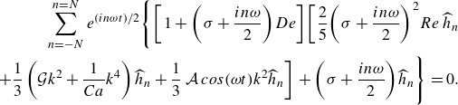 \begin{equation} \begin{aligned} \sum _{n=-N}^{n=N} e^{(in\omega t)/2}\Bigg \{\bigg [1+\bigg (\sigma +\frac {i n \omega }{2}\bigg ) De\bigg ]\bigg [\frac {2}{5} \bigg (\sigma + \frac {i n \omega }{2}\bigg )^2 Re\,\widehat {h}_n \\ +\frac {1}{3}\left (\mathcal{G} k^2 + \frac {1}{Ca} k^4 \right )\widehat {h}_n +\frac {1}{3}\,\mathcal{A}\,cos(\omega t)k^2 \widehat {h}_n\bigg ]+\bigg (\sigma + \frac {i n \omega }{2}\bigg )\widehat {h}_n\Bigg \}=0. \end{aligned} \end{equation}
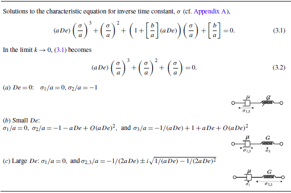
To get an algebraic expression that yields the inverse time constants, $\sigma$
, for a system subject to momentary disturbance, we set
$\sigma$
, for a system subject to momentary disturbance, we set $\mathcal{A}=0$
and
$\mathcal{A}=0$
and $\omega =0$
in (2.25), divide by
$\omega =0$
in (2.25), divide by $a$
and obtain
$a$
and obtain
 \begin{equation} (a De) \, \left (\frac {\sigma }{a}\right )^3+\left (\frac {\sigma }{a}\right )^2 + \, \left (1+\left [\frac {b}{a}\right ](a De)\right )\left (\frac {\sigma }{a}\right )+\left [\frac {b}{a}\right ]=0, \end{equation}
where the parameters $a$
and
$a$
and $b$
are given by
$b$
are given by
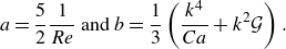 \begin{equation} a=\frac {5}{2}\frac {1}{Re} \text{ and } b=\frac {1}{3}\left (\frac {k^4}{Ca}+k^2 \mathcal{G}\right ). \end{equation}
Observe that the terms $(a De)$
, i.e.
$(a De)$
, i.e. $({5}/{2}) ({De}/{Re} )$
,
$({5}/{2}) ({De}/{Re} )$
, $ ({\sigma }/{a} )$
and
$ ({\sigma }/{a} )$
and $({b}/{a} )$
are independent of the characteristic time. The solutions to (2.26) for the inverse time constants are presented in table 1.
$({b}/{a} )$
are independent of the characteristic time. The solutions to (2.26) for the inverse time constants are presented in table 1.
Inverse-time constants at $\mathcal{A}=0$
and
$\mathcal{A}=0$
and $k=0$
for different
$k=0$
for different $De$
limits. Parameters
$De$
limits. Parameters $a$
and
$a$
and $b$
are given by (2.27).
$b$
are given by (2.27).
To get an algebraic expression determining the critical amplitude, $\mathcal{A}$
, for the dominant harmonic response, we set
$\mathcal{A}$
, for the dominant harmonic response, we set $\sigma =0$
in (2.25) and then employ a truncated Floquet expansion up to three terms for
$\sigma =0$
in (2.25) and then employ a truncated Floquet expansion up to three terms for $n=2,0$
and
$n=2,0$
and $-2$
, yielding (cf. (A26))
$-2$
, yielding (cf. (A26))
 \begin{equation} \mathcal{A}=\sqrt {6\Bigl (\frac {1}{Ca}+\frac {\mathcal{G}}{k^2 }\Bigr )\frac {[(\omega +De\omega c)^2+c^2]}{(1+De^2\omega ^2)c+De\omega ^2}}, \end{equation}
where $c=b-{\omega ^2}/{a}$
. In addition, this expression is used to provide useful insight into the interface’s temporal response as well as the stability characteristics of gravitationally unstable systems undergoing parametric forcing.
$c=b-{\omega ^2}/{a}$
. In addition, this expression is used to provide useful insight into the interface’s temporal response as well as the stability characteristics of gravitationally unstable systems undergoing parametric forcing.
3. Effect of elasticity on the fluid’s damping
The role of elasticity on the fluid’s damping can be understood by visualizing its behaviour as a simple spring–dashpot system (illustrated in table 1), with the stress–strain relationship given by (2.19). The viscoelastic fluid consists of a viscous component with viscosity, $\mu$
, represented by the dashpot, while the elastic component of shear modulus,
$\mu$
, represented by the dashpot, while the elastic component of shear modulus, $G$
, is represented by the spring. When the fluid system is subjected to a disturbance, the strain is distributed between the viscous and elastic components. If the value of
$G$
, is represented by the spring. When the fluid system is subjected to a disturbance, the strain is distributed between the viscous and elastic components. If the value of $G$
is large, i.e. at small values of Deborah numbers, the elastic component stores substantial normal and shear stresses while undergoing minimal deformation. Consequently, the main part of the deformation is undergone by the dashpot, leading to enhanced damping, dissipating the stresses acting on the system and thus stabilizing it. Conversely, at small values of
$G$
is large, i.e. at small values of Deborah numbers, the elastic component stores substantial normal and shear stresses while undergoing minimal deformation. Consequently, the main part of the deformation is undergone by the dashpot, leading to enhanced damping, dissipating the stresses acting on the system and thus stabilizing it. Conversely, at small values of $G$
or large Deborah numbers, the elastic component deforms more readily and the deformations undergone by the viscous component are reduced, thereby decreasing overall damping within the system. In the following section, we substantiate these statements by examining the values of the leading
$G$
or large Deborah numbers, the elastic component deforms more readily and the deformations undergone by the viscous component are reduced, thereby decreasing overall damping within the system. In the following section, we substantiate these statements by examining the values of the leading $\sigma$
for
$\sigma$
for $\mathcal{A}=0$
for different values of
$\mathcal{A}=0$
for different values of $G$
by considering three cases:
$G$
by considering three cases: $De=0$
(a Newtonian fluid); small Deborah numbers (i.e. a weakly elastic fluid); large Deborah numbers (i.e. a dominantly elastic fluid).
$De=0$
(a Newtonian fluid); small Deborah numbers (i.e. a weakly elastic fluid); large Deborah numbers (i.e. a dominantly elastic fluid).
3.1. Newtonian fluids: De=0
Analytical solutions for $\sigma$
in the case of a Newtonian liquid can be obtained by setting
$\sigma$
in the case of a Newtonian liquid can be obtained by setting $De=0$
in the characteristic equation (3.1) given in table 1 and solving for the resulting quadratic roots. This yields
$De=0$
in the characteristic equation (3.1) given in table 1 and solving for the resulting quadratic roots. This yields
 \begin{equation} \frac {\sigma _{1,2}}{a}=-\frac {1}{2}\pm i\sqrt {\frac {b}{a}-\frac {1}{4}}, \end{equation}
where the real part of ${\sigma }/{a}$
, which is independent of the characteristic time, gives the decay rate of the disturbances and the imaginary part, its natural frequency.
${\sigma }/{a}$
, which is independent of the characteristic time, gives the decay rate of the disturbances and the imaginary part, its natural frequency.
Observe that for gravitationally stable configurations, i.e. when ${b}/{a}\gt 0$
, both roots have a negative real part. Such a system is stable due to the viscous dissipative effects that dampen all disturbances. However, for gravitationally unstable configurations, i.e. when
${b}/{a}\gt 0$
, both roots have a negative real part. Such a system is stable due to the viscous dissipative effects that dampen all disturbances. However, for gravitationally unstable configurations, i.e. when ${b}/{a}\lt 0$
, we obtain two real roots, one root being positive, other being negative. The interface of such a system grows with time.
${b}/{a}\lt 0$
, we obtain two real roots, one root being positive, other being negative. The interface of such a system grows with time.
3.2.
Viscoelastic fluids: $De\neq 0$

If $De \neq 0$
, the characteristic cubic equation (3.1) exhibits three solutions, where the additional
$De \neq 0$
, the characteristic cubic equation (3.1) exhibits three solutions, where the additional $\sigma$
arises from the time derivative in the stress-strain constitutive equation (2.19). While solutions to these cubic equations may be rigorously obtained, we can easily derive expressions for the real parts of
$\sigma$
arises from the time derivative in the stress-strain constitutive equation (2.19). While solutions to these cubic equations may be rigorously obtained, we can easily derive expressions for the real parts of $\sigma$
in the limit
$\sigma$
in the limit $k \to 0$
. These expressions, also given in table 1, will be employed to elucidate the impact of elasticity on the fluid’s damping in the next two subsections.
$k \to 0$
. These expressions, also given in table 1, will be employed to elucidate the impact of elasticity on the fluid’s damping in the next two subsections.
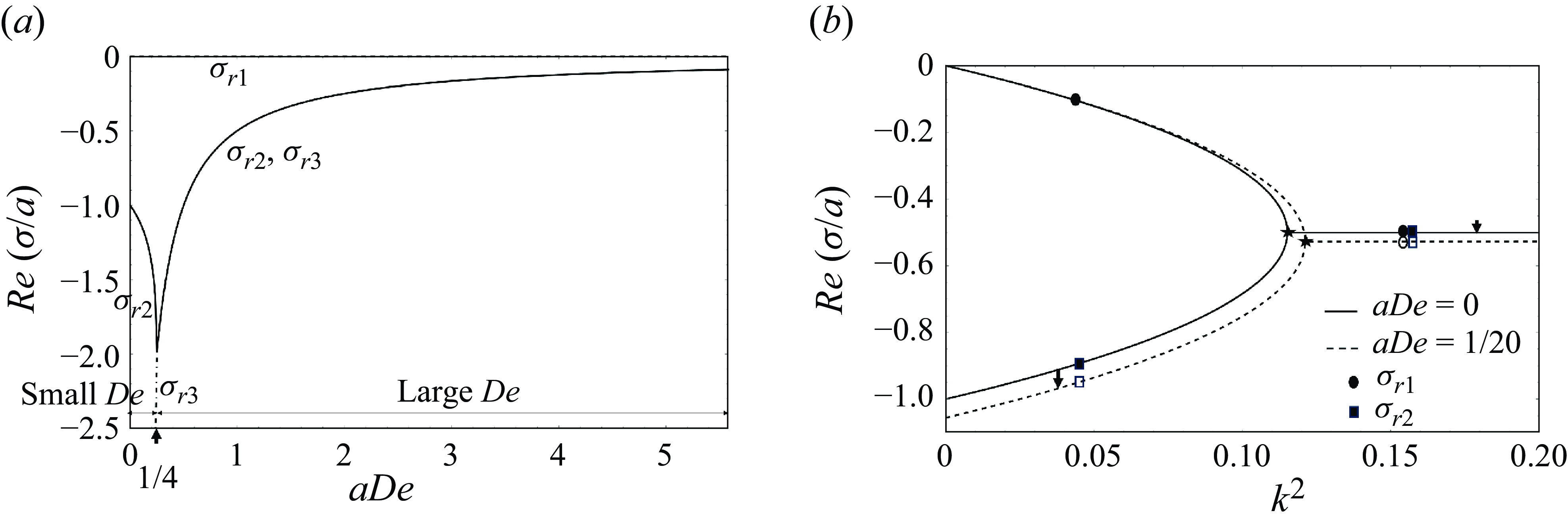
3.2.1. Low Deborah numbers or weakly elastic fluids
Consider the effect of elasticity for small Deborah numbers. Recall, from the example of a spring–dashpot system that, at small $De$
, damping is enhanced. This is evident by the trends shown by
$De$
, damping is enhanced. This is evident by the trends shown by $\sigma _1$
and
$\sigma _1$
and $\sigma _2$
in the limit
$\sigma _2$
in the limit $k\to 0$
(cf. table 1(b)) and depicted in figure 2(a) where we plot the real part of
$k\to 0$
(cf. table 1(b)) and depicted in figure 2(a) where we plot the real part of $\sigma /a$
, denoted
$\sigma /a$
, denoted $Re(\sigma /a)$
, versus
$Re(\sigma /a)$
, versus $(a De)$
, two quantities that are independent of the characteristic time. The root,
$(a De)$
, two quantities that are independent of the characteristic time. The root, $\sigma _3$
, is real and negative, the implication being it cannot influence an oscillatory Faraday instability threshold when the system is subjected to parametric forcing. However, we can see by computations that
$\sigma _3$
, is real and negative, the implication being it cannot influence an oscillatory Faraday instability threshold when the system is subjected to parametric forcing. However, we can see by computations that $\sigma _1$
and
$\sigma _1$
and $\sigma _2$
, although real as
$\sigma _2$
, although real as $k\to 0$
, become complex conjugates beyond a threshold wavenumber,
$k\to 0$
, become complex conjugates beyond a threshold wavenumber, $k$
, that depends on the value of
$k$
, that depends on the value of $(a De)$
,
$(a De)$
, $(\mathcal{G}/a)$
and
$(\mathcal{G}/a)$
and $a Ca$
, quantities that are also independent of the characteristic time. This result is depicted in figure 2(b). Observe that as
$a Ca$
, quantities that are also independent of the characteristic time. This result is depicted in figure 2(b). Observe that as $k$
approaches zero,
$k$
approaches zero, $\sigma _1$
approaches zero and
$\sigma _1$
approaches zero and $\sigma _2$
becomes more negative as
$\sigma _2$
becomes more negative as $De$
increases, implying that overall damping within the system increases with an increase in elasticity. This behaviour continues even when
$De$
increases, implying that overall damping within the system increases with an increase in elasticity. This behaviour continues even when $k$
is increased and
$k$
is increased and $\sigma _{1,2}$
become complex, thereby showing an increase in the Faraday instability threshold for an increase in
$\sigma _{1,2}$
become complex, thereby showing an increase in the Faraday instability threshold for an increase in $De$
in the low Deborah number regime.
$De$
in the low Deborah number regime.
(a) The real part of ${\sigma }/{a}$
, denoted
${\sigma }/{a}$
, denoted $Re({\sigma }/{a})$
, versus
$Re({\sigma }/{a})$
, versus $a De$
from (3.2). The arrow denotes the location beyond which
$a De$
from (3.2). The arrow denotes the location beyond which $\sigma _2$
and
$\sigma _2$
and $\sigma _3$
become complex conjugates. (b) Here
$\sigma _3$
become complex conjugates. (b) Here $Re({\sigma }/{a})$
versus
$Re({\sigma }/{a})$
versus $k^2$
for two different values of
$k^2$
for two different values of $(a De)$
in low Deborah number regime for parameters
$(a De)$
in low Deborah number regime for parameters $a Ca=5.3$
and
$a Ca=5.3$
and $\mathcal{G}/a=0.63$
, corresponding to the properties of a fluid given in table 2. The inverse time constant,
$\mathcal{G}/a=0.63$
, corresponding to the properties of a fluid given in table 2. The inverse time constant, $\sigma _3$
, which has very large negative values at low
$\sigma _3$
, which has very large negative values at low $De$
is not shown here. The symbol
$De$
is not shown here. The symbol $\star$
denotes the location beyond which
$\star$
denotes the location beyond which $\sigma _1$
and
$\sigma _1$
and $\sigma _2$
become complex conjugates.
$\sigma _2$
become complex conjugates.
Physical parameters used in the calculations. Fluid properties correspond to $0.5\,\%$
wt./vol. aqueous polyacrylamide solution (Sobti et al. Reference Sobti, Toor and Wanchoo2018) making
$0.5\,\%$
wt./vol. aqueous polyacrylamide solution (Sobti et al. Reference Sobti, Toor and Wanchoo2018) making $De/Re=2$
, which is independent of any timescale.
$De/Re=2$
, which is independent of any timescale.
3.2.2. Large Deborah numbers or strongly elastic fluids
Contrasting the case of a low Deborah number with that of large $De$
, we observe that now the decay rates decrease with an increase in
$De$
, we observe that now the decay rates decrease with an increase in $De$
. This is depicted in figure 2(a) and supported by the equations given in case (c) of table 1, from which we also see that when
$De$
. This is depicted in figure 2(a) and supported by the equations given in case (c) of table 1, from which we also see that when $(aDe)\gt 1/4$
, i.e.
$(aDe)\gt 1/4$
, i.e. $De/Re\gt 1/10$
,
$De/Re\gt 1/10$
, $\sigma _2$
and
$\sigma _2$
and $\sigma _3$
are complex conjugates, their real parts being inversely proportional to
$\sigma _3$
are complex conjugates, their real parts being inversely proportional to $De$
. Therefore, for large
$De$
. Therefore, for large $De$
, the elasticity-induced inertia reduces the stability of the system, i.e. making it more susceptible to Faraday instability.
$De$
, the elasticity-induced inertia reduces the stability of the system, i.e. making it more susceptible to Faraday instability.
The behaviour of $\sigma$
values with
$\sigma$
values with $De$
as discussed above and its implication in Faraday instability is delineated in two cases. These are parametric forcing on a gravitationally stable system and forcing on a gravitationally unstable system. We turn to these two cases in the following sections.
$De$
as discussed above and its implication in Faraday instability is delineated in two cases. These are parametric forcing on a gravitationally stable system and forcing on a gravitationally unstable system. We turn to these two cases in the following sections.
4. Parametric forcing of a viscoelastic fluid in a gravitationally stable orientation
4.1. Relating the behaviour of the Faraday instability to the inverse time constants
In the last section, it was hypothesized that damping rates ought to be connected to the stability threshold of resonant instability. To verify this, we examine the stability characteristics by considering a viscoelastic fluid whose properties are given in table 2, focusing on the case of a gravitationally stable system where $g=9.8\, m\,s^{-2}$
, i.e Earth’s gravity level. Linear stability calculations are performed using the complete set of equations (2.17) to (2.23) for arbitrary wavenumbers,
$g=9.8\, m\,s^{-2}$
, i.e Earth’s gravity level. Linear stability calculations are performed using the complete set of equations (2.17) to (2.23) for arbitrary wavenumbers, $k$
.
$k$
.
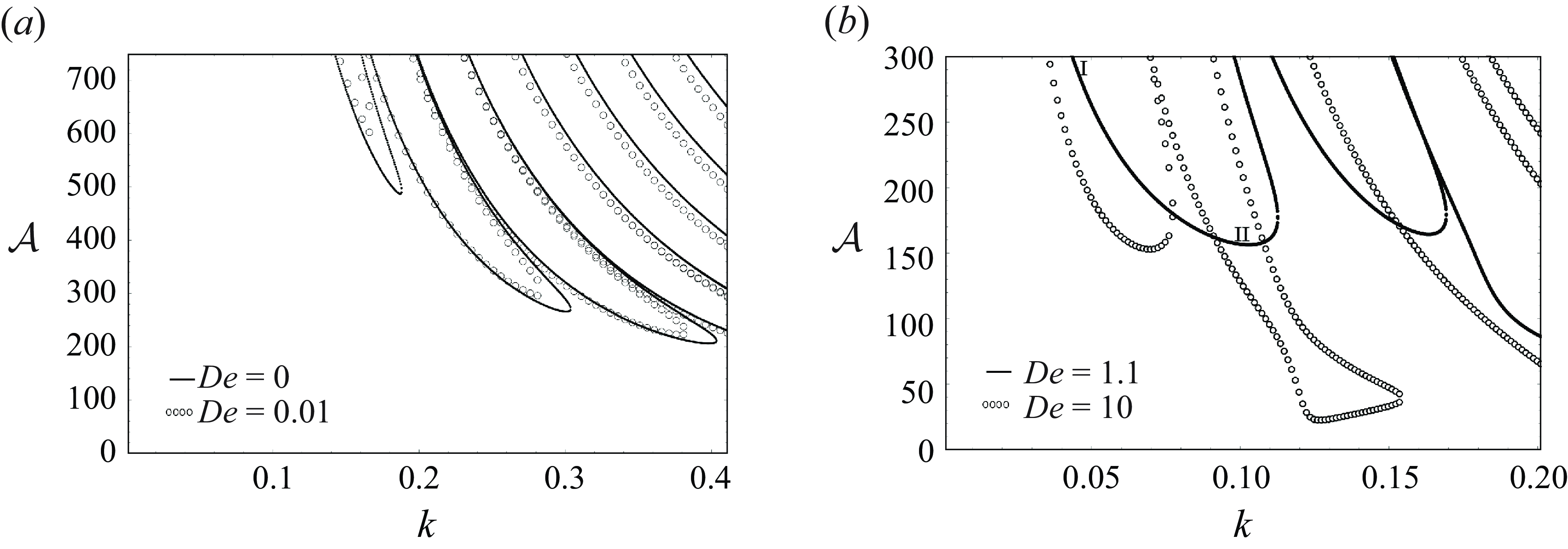
In a weakly viscoelastic fluid, we noted in § 3 that there is increased damping due to elasticity. This, in turn leads to increased threshold amplitudes for the onset of Faraday instability as illustrated in the $\mathcal{A}$
versus
$\mathcal{A}$
versus $k$
graphs of figure 3(a). These graphs are plotted for two different values of Deborah number in the low Deborah number region, viz.,
$k$
graphs of figure 3(a). These graphs are plotted for two different values of Deborah number in the low Deborah number region, viz., $De=0$
and
$De=0$
and $De=0.01$
, reflecting a change only in the shear modulus in table 2. Henceforth we take the characteristic velocity to be
$De=0.01$
, reflecting a change only in the shear modulus in table 2. Henceforth we take the characteristic velocity to be
 \begin{equation} U\equiv d^* \omega ^*, \end{equation}
thus requiring the scaled frequency to be $\omega =1$
, from (2.8).
$\omega =1$
, from (2.8).
By contrast with a low $De$
region, we observed in § 3 that at large
$De$
region, we observed in § 3 that at large $De$
there is a decrease in the damping rate with an increase in
$De$
there is a decrease in the damping rate with an increase in $De$
(cf. figure 2
a). This implies that the threshold amplitude for the Faraday instability ought to decrease with an increase in
$De$
(cf. figure 2
a). This implies that the threshold amplitude for the Faraday instability ought to decrease with an increase in $De$
due to the inertia-like action provided by elasticity. This is illustrated by the results in figure 3(b). A significant reduction in critical amplitude is shown for this case in the figure where
$De$
due to the inertia-like action provided by elasticity. This is illustrated by the results in figure 3(b). A significant reduction in critical amplitude is shown for this case in the figure where $\mathcal{A}$
versus
$\mathcal{A}$
versus $k$
is plotted for two different values of Deborah numbers, viz.,
$k$
is plotted for two different values of Deborah numbers, viz., $De=1.1$
and
$De=1.1$
and $De=10$
. The value
$De=10$
. The value $G=1.55\,\textit{Pa}$
given in table 2 for a realistic fluid corresponds to
$G=1.55\,\textit{Pa}$
given in table 2 for a realistic fluid corresponds to $De=1.1$
, placing it within the large Deborah number category. Observe in figure 3(b) that there is a noticeable difference in the shape of the second tongue and subsequent tongues (not shown), as we transit from
$De=1.1$
, placing it within the large Deborah number category. Observe in figure 3(b) that there is a noticeable difference in the shape of the second tongue and subsequent tongues (not shown), as we transit from $De=1.1$
to
$De=1.1$
to $De=10$
, where the elasticity of the fluid becomes dominant. This difference is attributed to the memory effect imparted by the fluid’s elasticity as characterized by the change in the relaxation time of the fluid. The core characteristics of the stability curves, however, remain unchanged, such as the alternating subharmonic and harmonic responses.
$De=10$
, where the elasticity of the fluid becomes dominant. This difference is attributed to the memory effect imparted by the fluid’s elasticity as characterized by the change in the relaxation time of the fluid. The core characteristics of the stability curves, however, remain unchanged, such as the alternating subharmonic and harmonic responses.
Critical $\mathcal{A}$
versus
$\mathcal{A}$
versus $k$
curves, shows the effect of elasticity on the Faraday instability threshold at
$k$
curves, shows the effect of elasticity on the Faraday instability threshold at $g= 9.8\,\rm m\, s^{-2}$
. (a) The solid curve represents
$g= 9.8\,\rm m\, s^{-2}$
. (a) The solid curve represents $De=0$
and the open circle markers represent
$De=0$
and the open circle markers represent $De=0.01$
(b) The solid curve
$De=0.01$
(b) The solid curve $De=1.1$
and the open circle markers represent
$De=1.1$
and the open circle markers represent $De=10$
. The dimensional frequency,
$De=10$
. The dimensional frequency, $\omega ^*=2 \pi\,\rm rad\,s^{-1}$
and
$\omega ^*=2 \pi\,\rm rad\,s^{-1}$
and $f^*=1\,\rm Hz$
.
$f^*=1\,\rm Hz$
.
4.2. The temporal response of the interface due to Faraday instability
Just as the real part of $\sigma$
informs us about the behaviour of the Faraday threshold, the imaginary part of
$\sigma$
informs us about the behaviour of the Faraday threshold, the imaginary part of $\sigma$
provides information about the interface’s temporal response. Recall, from the earlier section that we obtain three roots to
$\sigma$
provides information about the interface’s temporal response. Recall, from the earlier section that we obtain three roots to $\sigma$
when (3.1) is solved, yielding two complex conjugate roots and one purely negative root, for a wavenumber,
$\sigma$
when (3.1) is solved, yielding two complex conjugate roots and one purely negative root, for a wavenumber, $k$
, above a minimum value as depicted in figure 2(b). The very existence of complex
$k$
, above a minimum value as depicted in figure 2(b). The very existence of complex $\sigma$
suggests the possibility of an oscillatory response upon resonant instability, as observed in the case of Newtonian fluids (Kumar & Tuckerman Reference Kumar and Tuckerman1994). On the other hand, the presence of a purely negative
$\sigma$
suggests the possibility of an oscillatory response upon resonant instability, as observed in the case of Newtonian fluids (Kumar & Tuckerman Reference Kumar and Tuckerman1994). On the other hand, the presence of a purely negative $\sigma$
, indicates the possibility of a monotonic response. We shall show that such a response is indeed possible and becomes dominant compared with an oscillatory instability for large
$\sigma$
, indicates the possibility of a monotonic response. We shall show that such a response is indeed possible and becomes dominant compared with an oscillatory instability for large $De$
as gravity approaches zero.
$De$
as gravity approaches zero.
To determine the temporal response of the instability we revisit the $\mathcal{A}$
versus
$\mathcal{A}$
versus $k$
graph represented by the solid curve in figure 3(b), i.e. for
$k$
graph represented by the solid curve in figure 3(b), i.e. for $De=1.1$
and
$De=1.1$
and $g=$
9.8 m s
$g=$
9.8 m s $^{-2}$
. The graph depicts a critical curve consisting of multiple ‘tongues’, each associated with distinctive temporal modes. Typically, the interface response at the onset of instability corresponds to the temporal mode with the lowest of all the critical amplitudes. The nature of the temporal response of the interface at a given critical amplitude,
$^{-2}$
. The graph depicts a critical curve consisting of multiple ‘tongues’, each associated with distinctive temporal modes. Typically, the interface response at the onset of instability corresponds to the temporal mode with the lowest of all the critical amplitudes. The nature of the temporal response of the interface at a given critical amplitude, $\mathcal{A}$
, is determined by examining the coefficients,
$\mathcal{A}$
, is determined by examining the coefficients, $\widehat {h}_n$
, in the Floquet summation (2.24). If the dominant coefficient corresponds to
$\widehat {h}_n$
, in the Floquet summation (2.24). If the dominant coefficient corresponds to $n=0$
, the response is said to be monotonic. Otherwise, it is an oscillatory response. Among the oscillatory modes, depending on whether the dominant coefficient is odd or even, the interface response is either subharmonic or harmonic. We note that higher-order subharmonics may occur when the dominant coefficient corresponds to
$n=0$
, the response is said to be monotonic. Otherwise, it is an oscillatory response. Among the oscillatory modes, depending on whether the dominant coefficient is odd or even, the interface response is either subharmonic or harmonic. We note that higher-order subharmonics may occur when the dominant coefficient corresponds to $n=3,5,7,$
etc. And higher-order harmonics may occur when
$n=3,5,7,$
etc. And higher-order harmonics may occur when $n=4,6,8,$
etc. As an example, the response of the interface deformation is subharmonic at the minimum of the second tongue (cf. solid curves in figure 3
b) as all the even coefficients are zero and the indices of the dominant coefficients are odd. On the other hand, the response of the interface deformation at the minimum of the first tongue is harmonic as all the odd coefficients are zero and the indices in the dominant coefficients are even. Although not displayed in figure 3(b), our calculations show that for
$n=4,6,8,$
etc. As an example, the response of the interface deformation is subharmonic at the minimum of the second tongue (cf. solid curves in figure 3
b) as all the even coefficients are zero and the indices of the dominant coefficients are odd. On the other hand, the response of the interface deformation at the minimum of the first tongue is harmonic as all the odd coefficients are zero and the indices in the dominant coefficients are even. Although not displayed in figure 3(b), our calculations show that for $De \sim 1$
, we observe a transition between subharmonic and harmonic responses, in agreement with earlier works (Kumar Reference Kumar1999; Müller & Zimmermann Reference Müller and Zimmermann1999). It is noteworthy that earlier workers have also observed a harmonic response in parametric forcing in the case of soft solids (Bevilacqua et al. Reference Bevilacqua, Shao, Saylor, Bostwick and Ciarletta2020).
$De \sim 1$
, we observe a transition between subharmonic and harmonic responses, in agreement with earlier works (Kumar Reference Kumar1999; Müller & Zimmermann Reference Müller and Zimmermann1999). It is noteworthy that earlier workers have also observed a harmonic response in parametric forcing in the case of soft solids (Bevilacqua et al. Reference Bevilacqua, Shao, Saylor, Bostwick and Ciarletta2020).
The relative importance of a monotonic response with respect to a first harmonic response in the first tongue may be estimated from the ratio obtained using a three-term Floquet summation of the reduced-order model, i.e. when $\epsilon {\ll }1$
. The details of such a model are given in Appendix A, where, from (A27) we obtain
$\epsilon {\ll }1$
. The details of such a model are given in Appendix A, where, from (A27) we obtain
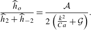 \begin{equation} \frac {\widehat {h}_o}{\widehat {h}_2+\widehat {h}_{-2}}=\frac {\mathcal{A}}{2\left (\frac {k^2}{Ca}+\mathcal{G}\right )}. \end{equation}
The corresponding critical amplitude, $\mathcal{A}$
, obtained from (2.28), is given by
$\mathcal{A}$
, obtained from (2.28), is given by
 \begin{equation} \mathcal{A}=\sqrt {6\Bigl (\frac {1}{Ca}+\frac {\mathcal{G}}{k^2 }\Bigr )\frac {[(1+c De )^2+c^2]}{(1+De^2)c+De},} \end{equation}
where $c(k)=b(k)-\frac {1}{a}$
, and where
$c(k)=b(k)-\frac {1}{a}$
, and where $a$
and
$a$
and $b$
are given by (2.27). Recall that the dimensionless frequency,
$b$
are given by (2.27). Recall that the dimensionless frequency, $\omega$
, is equal to one. Observe that as
$\omega$
, is equal to one. Observe that as $k$
goes to zero, the ratio
$k$
goes to zero, the ratio $\widehat {h}_0/(\widehat {h}_2+\widehat {h}_{-2})$
and the critical amplitude,
$\widehat {h}_0/(\widehat {h}_2+\widehat {h}_{-2})$
and the critical amplitude, $\mathcal{A}$
, approach infinity provided
$\mathcal{A}$
, approach infinity provided $\mathcal{G}\gt 0$
. In figure 3(b), this region, where the monotonic mode is dominant corresponds to the descending region in the first critical curve, denoted
$\mathcal{G}\gt 0$
. In figure 3(b), this region, where the monotonic mode is dominant corresponds to the descending region in the first critical curve, denoted $\textrm {I}$
. However, as
$\textrm {I}$
. However, as $k$
increases, i.e. as we approach the minima of the first critical curve, denoted
$k$
increases, i.e. as we approach the minima of the first critical curve, denoted $\textrm {II}$
, the harmonic modes become important. It should be noted that the monotonic behaviour for curves characterized by
$\textrm {II}$
, the harmonic modes become important. It should be noted that the monotonic behaviour for curves characterized by $De=1.1$
will also occur for curves with different shear moduli,
$De=1.1$
will also occur for curves with different shear moduli, $G$
, but at a different parametric frequency.
$G$
, but at a different parametric frequency.
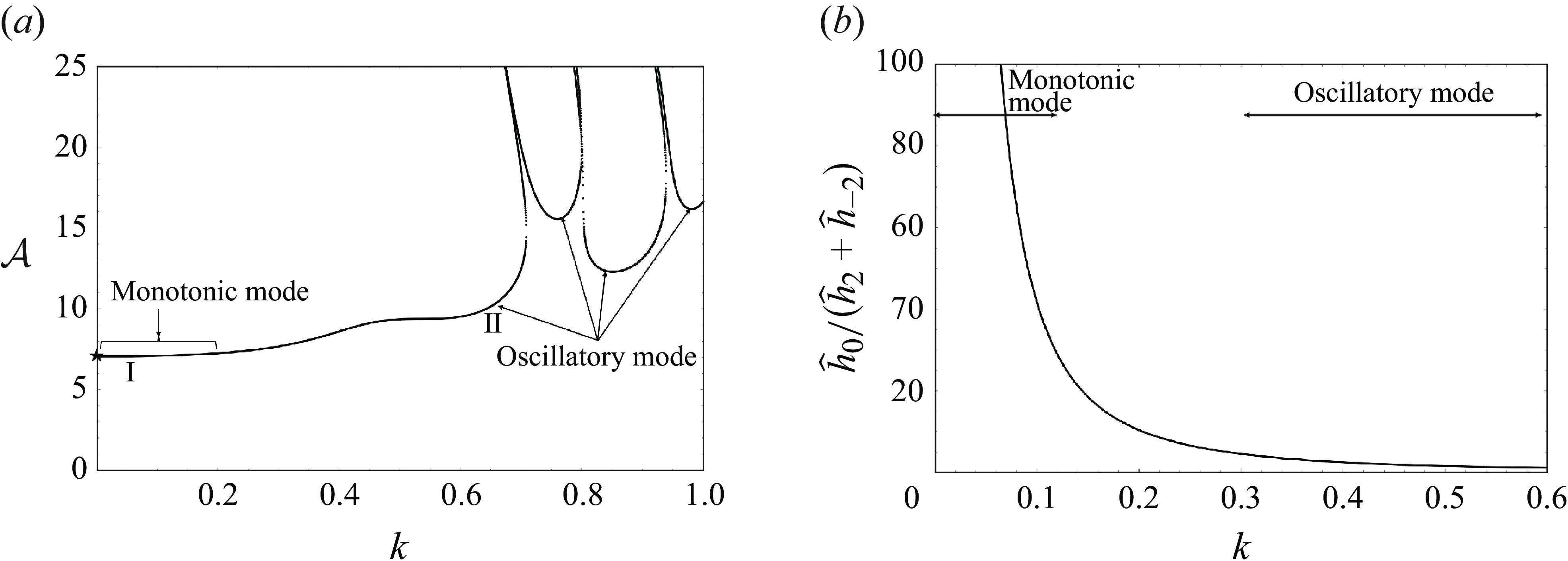
Now, as $\mathcal{G}$
is reduced, the region
$\mathcal{G}$
is reduced, the region $\textrm {I}$
of the curve shifts downward faster than the region
$\textrm {I}$
of the curve shifts downward faster than the region $\textrm {II}$
and all other regions, subsequently becoming the most unstable mode with the lowest critical amplitude at
$\textrm {II}$
and all other regions, subsequently becoming the most unstable mode with the lowest critical amplitude at $\mathcal{G}=0$
. This is illustrated in figure 4(a) where the lowest amplitude corresponds to the point where the curve touches the ordinate (marked by a star), i.e.
$\mathcal{G}=0$
. This is illustrated in figure 4(a) where the lowest amplitude corresponds to the point where the curve touches the ordinate (marked by a star), i.e. $k=0$
. Indeed, the ratio
$k=0$
. Indeed, the ratio $\widehat {h}_0/(\widehat {h}_2+\widehat {h}_{-2})$
versus
$\widehat {h}_0/(\widehat {h}_2+\widehat {h}_{-2})$
versus $k$
graph plotted in figure 4(b) shows that the monotonic behaviour of the system increases with a decrease in wavenumber and eventually becomes purely monotonic at
$k$
graph plotted in figure 4(b) shows that the monotonic behaviour of the system increases with a decrease in wavenumber and eventually becomes purely monotonic at $k=0$
. The critical amplitude as
$k=0$
. The critical amplitude as $k$
approaches zero can be accurately determined using the expression for
$k$
approaches zero can be accurately determined using the expression for $\mathcal{A}$
from (4.3). This expression is in good agreement with figure 4(a) in the limit of small wavenumbers (see the figure in Appendix A).
$\mathcal{A}$
from (4.3). This expression is in good agreement with figure 4(a) in the limit of small wavenumbers (see the figure in Appendix A).
The existence of a monotonic Faraday instability mode, depicted by graphs using the properties of the fluid given in table 2 with $\mathcal{G}=0$
(a) Critical
$\mathcal{G}=0$
(a) Critical $\mathcal{A}$
versus
$\mathcal{A}$
versus $k$
. (b) The ratio
$k$
. (b) The ratio $\widehat {h}_0/(\widehat {h}_2+\widehat {h}_{-2})$
versus
$\widehat {h}_0/(\widehat {h}_2+\widehat {h}_{-2})$
versus $k$
obtained using (4.2). The dimensional frequency,
$k$
obtained using (4.2). The dimensional frequency, $\omega ^*=2 \pi\,\rm rad\, s^{-1}$
and
$\omega ^*=2 \pi\,\rm rad\, s^{-1}$
and $f^*=1\,\rm Hz$
.
$f^*=1\,\rm Hz$
.
4.3.
Criteria for the existence of a purely monotonic faraday instability at
$\mathcal{G}=0$

The criteria for the existence of purely monotonic instability can be derived by requiring that $De$
and
$De$
and $Re$
be such that (4.3) yields a real value of
$Re$
be such that (4.3) yields a real value of $\mathcal{A}$
as
$\mathcal{A}$
as $k\to 0$
. Doing this results in the criteria taking the form
$k\to 0$
. Doing this results in the criteria taking the form
 \begin{equation} \frac {De}{1+De^2}\gt \frac {2 }{5}Re, \end{equation}
an inequality that is derived in Appendix A (cf. (A29)). It can be observed from (4.4) that the left-hand side reaches a maximum at $De=1$
, i.e. when the forcing frequency is the inverse of the relaxation time. At this value of
$De=1$
, i.e. when the forcing frequency is the inverse of the relaxation time. At this value of $De$
, the left-hand side of (4.4) is
$De$
, the left-hand side of (4.4) is $1/2$
and
$1/2$
and $Re\lt 5/4$
. Thus, to get a monotonic mode,
$Re\lt 5/4$
. Thus, to get a monotonic mode, $Re$
must depend on this condition but must not exceed
$Re$
must depend on this condition but must not exceed $5/4$
, i.e. the inertia due to momentum must be weak.
$5/4$
, i.e. the inertia due to momentum must be weak.
At high $Re$
, such that (4.4) is not satisfied, the fluid interface exhibits oscillatory behaviour because the viscous damping within the system is reduced. However, even at low
$Re$
, such that (4.4) is not satisfied, the fluid interface exhibits oscillatory behaviour because the viscous damping within the system is reduced. However, even at low $Re$
, i.e. if
$Re$
, i.e. if $Re\lt 5/4$
, but high
$Re\lt 5/4$
, but high $De$
i.e. if
$De$
i.e. if $De\gt 1$
, (4.4) will also not be satisfied and the response of the interface will be oscillatory because of the elasticity-induced inertia.
$De\gt 1$
, (4.4) will also not be satisfied and the response of the interface will be oscillatory because of the elasticity-induced inertia.
We can use the criteria given in the relationship given by (4.4), to determine bounds on $G$
,
$G$
, $\mu$
and
$\mu$
and $\omega ^*$
. As an example, for assigned values of
$\omega ^*$
. As an example, for assigned values of $\mu$
,
$\mu$
, $\omega ^*$
, etc., we can obtain
$\omega ^*$
, etc., we can obtain $G$
from
$G$
from $De$
by a rearrangement of relationship (4.4), viz.
$De$
by a rearrangement of relationship (4.4), viz.
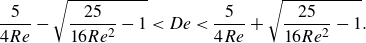 \begin{equation} \frac {5}{4 Re }-\sqrt {\frac {25}{16 Re^2 }-1}\lt De\lt \frac {5}{4 Re }+\sqrt {\frac {25}{16 Re^2}-1}. \end{equation}
Likewise, we can obtain $\mu$
from
$\mu$
from $Re$
with another rearrangement of (4.4), i.e.
$Re$
with another rearrangement of (4.4), i.e.
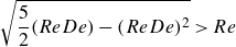 \begin{equation} \sqrt {\frac {5}{2}(Re De)-(ReDe)^2}\gt Re \end{equation}
for assigned values of $G$
,
$G$
, $\omega ^*$
, etc. Finally, for assigned values of
$\omega ^*$
, etc. Finally, for assigned values of $\mu$
,
$\mu$
, $G$
, etc., we may estimate the values of the dimensional frequency,
$G$
, etc., we may estimate the values of the dimensional frequency, $\omega ^{*}$
, from
$\omega ^{*}$
, from $Re$
with one more rearrangement of (4.4) as
$Re$
with one more rearrangement of (4.4) as
 \begin{equation} \frac {\sqrt {\frac {5}{2}\frac {De}{Re}-1}}{\frac {De}{Re}}\gt Re \end{equation}
observing that $De/Re$
is independent of
$De/Re$
is independent of $\omega ^*$
. These bounds on
$\omega ^*$
. These bounds on $G$
,
$G$
, $\mu$
and
$\mu$
and $\omega ^*$
are also illustrated using the phase diagrams shown in figures 5(a) and 5(b). In both graphs, the intersection of the horizontal and vertical dashed lines marked by ‘
$\omega ^*$
are also illustrated using the phase diagrams shown in figures 5(a) and 5(b). In both graphs, the intersection of the horizontal and vertical dashed lines marked by ‘ $\star$
’ indicates the parameter values used to generate figure 4(a), depicting the presence of a purely monotonic mode. Observe that the maximum value of
$\star$
’ indicates the parameter values used to generate figure 4(a), depicting the presence of a purely monotonic mode. Observe that the maximum value of $Re$
,
$Re$
, $Re=5/4$
, above which monotonic instability cannot occur, a result that we derived earlier from (4.4), is also denoted on figures 5(a) and 5(b).
$Re=5/4$
, above which monotonic instability cannot occur, a result that we derived earlier from (4.4), is also denoted on figures 5(a) and 5(b).
Phase diagrams illustrating the parameter ranges within which a purely monotonic mode exists at $\mathcal{G}=0$
. (a) Here
$\mathcal{G}=0$
. (a) Here $Re$
versus
$Re$
versus $DeRe$
, determining the bounds of
$DeRe$
, determining the bounds of $\mu$
for fixed
$\mu$
for fixed $G$
and
$G$
and $\omega ^*$
from (4.6). (b) Here
$\omega ^*$
from (4.6). (b) Here $Re$
versus
$Re$
versus $De/Re$
, determining the bounds of
$De/Re$
, determining the bounds of $\omega ^*$
for a fixed
$\omega ^*$
for a fixed $G$
and
$G$
and $\mu$
from (4.7).
$\mu$
from (4.7).
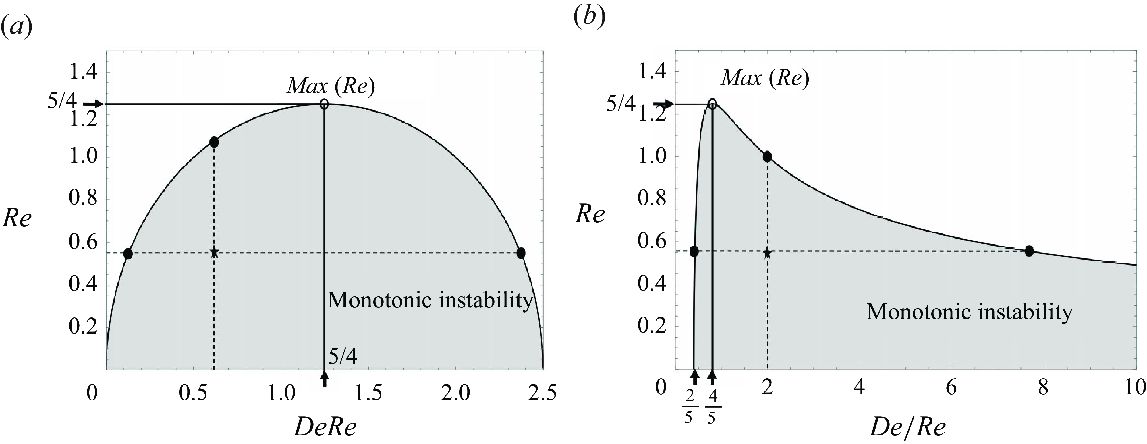
Using the properties of a viscoelastic fluid given in table 2 in the relationship (4.7), we can see that the pure monotonic mode occurs for frequencies of forcing, less than $1.8{\,\rm Hz}$
. This cutoff frequency can also be obtained from the graph in figure 5(b) by calculating
$1.8{\,\rm Hz}$
. This cutoff frequency can also be obtained from the graph in figure 5(b) by calculating $\omega ^*$
from
$\omega ^*$
from $Re$
at
$Re$
at $De/Re=2$
(marked by
$De/Re=2$
(marked by $\bullet$
). Beyond this frequency, pure monotonic instability does not exist, though a predominantly monotonic response is still observed near this critical frequency. As the forcing frequency is increased further, the instability response changes to a dominantly oscillatory behaviour.
$\bullet$
). Beyond this frequency, pure monotonic instability does not exist, though a predominantly monotonic response is still observed near this critical frequency. As the forcing frequency is increased further, the instability response changes to a dominantly oscillatory behaviour.
To ensure that disturbances are in the low wavenumber limit, the finiteness of the container must be taken into account. For example, in containers of finite width, $W$
, and with stress-free sidewalls, we have a set of allowable wavenumbers,
$W$
, and with stress-free sidewalls, we have a set of allowable wavenumbers, $k$
, where
$k$
, where $k = m\pi /W$
, with
$k = m\pi /W$
, with $m{\in }\mathbb{N}$
. Consequently, in a narrow container, only shorter waveforms leading to oscillatory instability will occur as the permissible wavenumber belongs to the large wavenumber region (cf. figure 4
a). However, in wide containers long wavelength waveforms will develop, leading to a dominantly monotonic instability.
$m{\in }\mathbb{N}$
. Consequently, in a narrow container, only shorter waveforms leading to oscillatory instability will occur as the permissible wavenumber belongs to the large wavenumber region (cf. figure 4
a). However, in wide containers long wavelength waveforms will develop, leading to a dominantly monotonic instability.
The occurrence of a monotonic response, a new observation in parametric forcing of viscoelastic fluids is thus attributed to the inverse time constant, $\sigma$
, which is purely real. It might be of related interest to note that other monotonic long-wave instabilities, such as the Rayleigh–Taylor (RT) instability of Newtonian fluids, are also characterized by purely real
$\sigma$
, which is purely real. It might be of related interest to note that other monotonic long-wave instabilities, such as the Rayleigh–Taylor (RT) instability of Newtonian fluids, are also characterized by purely real $\sigma$
. Further, such an instability may be stabilized by parametric forcing (Sterman-Cohen et al. Reference Sterman-Cohen, Bestehorn and Oron2017). This therefore encourages the question: Can the RT instability of a viscoelastic fluid be staved off upon parametric forcing? To answer this question we set
$\sigma$
. Further, such an instability may be stabilized by parametric forcing (Sterman-Cohen et al. Reference Sterman-Cohen, Bestehorn and Oron2017). This therefore encourages the question: Can the RT instability of a viscoelastic fluid be staved off upon parametric forcing? To answer this question we set $\mathcal{G}$
to be negative, i.e. with gravity now pointing upwards in figure 1, fix the container width, and then analyse the regions of stability/instability when parametric forcing is employed.
$\mathcal{G}$
to be negative, i.e. with gravity now pointing upwards in figure 1, fix the container width, and then analyse the regions of stability/instability when parametric forcing is employed.
5. Parametric forcing of a viscoelastic fluid in a gravitationally unstable orientation
Viscoelastic fluid layer in an RT arrangement (a) without forcing – neutral stability curve. The point $\star$
is the intersection between
$\star$
is the intersection between $B=0.1$
and
$B=0.1$
and $k=\pi /W$
(the first allowable wavenumber) and lies slightly above the neutral line (b) with forcing – stability bounds for the monotonic (s) and oscillatory (o) modes for
$k=\pi /W$
(the first allowable wavenumber) and lies slightly above the neutral line (b) with forcing – stability bounds for the monotonic (s) and oscillatory (o) modes for $B=0.1$
, width
$B=0.1$
, width $W=10$
,
$W=10$
, $De/Re=2$
. Integers between parentheses, (
$De/Re=2$
. Integers between parentheses, ( $m$
), identify the most unstable wavenumber
$m$
), identify the most unstable wavenumber $k{=}m\pi /W$
. The two critical frequencies,
$k{=}m\pi /W$
. The two critical frequencies, $f^*_{c1}$
and
$f^*_{c1}$
and $f^*_{c2}$
, are marked
$f^*_{c2}$
, are marked $\star$
and
$\star$
and $\circ$
, occurring where dashed and solid curves intersect.
$\circ$
, occurring where dashed and solid curves intersect.
A fluid that is in a gravitationally unstable configuration may be stabilized by restricting the disturbances to short enough wavelengths such that the surface tension force exceeds the gravitational force. This is the familiar RT problem (Chandrasekhar Reference Chandrasekhar1961). The neutral stability threshold is given by $B=k_c^2$
and depicted in figure 6(a), where
$B=k_c^2$
and depicted in figure 6(a), where $k_c$
is the cutoff wavenumber. Here,
$k_c$
is the cutoff wavenumber. Here, $B$
is the Bond number, given by
$B$
is the Bond number, given by $B=-\mathcal{G}Ca$
, where
$B=-\mathcal{G}Ca$
, where $B\gt 0$
and
$B\gt 0$
and $\mathcal{G}\lt 0$
, due to the reversal in direction of the gravity vector from that shown in figure 1. The relationship between
$\mathcal{G}\lt 0$
, due to the reversal in direction of the gravity vector from that shown in figure 1. The relationship between $B$
and
$B$
and $k_c^2$
depicted in figure 6(a) is unaffected by the fluid’s elasticity as observed from (2.17)–(2.23), when
$k_c^2$
depicted in figure 6(a) is unaffected by the fluid’s elasticity as observed from (2.17)–(2.23), when $\sigma$
,
$\sigma$
, $\mathcal{A}$
and
$\mathcal{A}$
and $\omega$
are set to zero. Above the critical line in figure 6(a), the fluid system is unstable. Therefore, in an unbounded container, the most unstable wavenumber is
$\omega$
are set to zero. Above the critical line in figure 6(a), the fluid system is unstable. Therefore, in an unbounded container, the most unstable wavenumber is $k=0$
and we always have instability. However, in finite-width containers, as noted earlier, the lowest allowable wavenumber is
$k=0$
and we always have instability. However, in finite-width containers, as noted earlier, the lowest allowable wavenumber is $k=\pi /W$
, marked by a vertical dashed line in figure 6(a). For Bond numbers less than
$k=\pi /W$
, marked by a vertical dashed line in figure 6(a). For Bond numbers less than $k^2\vert _{m=1}$
, we have stability.
$k^2\vert _{m=1}$
, we have stability.
It is known from earlier work that a Newtonian fluid in a RT unstable configuration can be stabilized by parametric forcing (Sterman-Cohen et al. Reference Sterman-Cohen, Bestehorn and Oron2017). Because the Faraday instability is inertia-driven, the transient nature of the stress–strain constitutive relationship in a viscoelastic fluid must necessarily affect the manner in which parametric forcing can stabilize an otherwise RT unstable configuration. In this section, we therefore discuss the effect of such forcing on a viscoelastic fluid layer whose properties are given in table 2.
To understand the salient features of parametric stabilization of our gravitationally unstable system we turn to figure 6(b), which depicts forcing amplitude versus frequency for an example case where $W=10$
and
$W=10$
and $B=0.1$
. The critical curves in figure 6(b) are displayed in dimensional form in order to show that the results are in a practically achievable range. The curves in the figure are obtained by computing the two lowest critical amplitudes amongst all allowable wavenumbers for each input parametric frequency. The critical values are then sorted based on their temporal response, the dashed curve indicating the monotonic mode denoted,
$B=0.1$
. The critical curves in figure 6(b) are displayed in dimensional form in order to show that the results are in a practically achievable range. The curves in the figure are obtained by computing the two lowest critical amplitudes amongst all allowable wavenumbers for each input parametric frequency. The critical values are then sorted based on their temporal response, the dashed curve indicating the monotonic mode denoted, $\mathcal{A}_s$
, where
$\mathcal{A}_s$
, where $s$
represents a steady or monotonic mode. The solid curves represent oscillatory modes with critical amplitudes denoted,
$s$
represents a steady or monotonic mode. The solid curves represent oscillatory modes with critical amplitudes denoted, $\mathcal{A}_o$
. These curves divide the
$\mathcal{A}_o$
. These curves divide the $A^*$
versus
$A^*$
versus $f^*$
graph into three regions of stability/instability, where
$f^*$
graph into three regions of stability/instability, where $f^{*}=\omega ^{*}/2\pi$
. Below the dashed curve, the viscoelastic fluid system is monotonically unstable, and above the solid curve, it will exhibit an oscillatory response. Outside of these regions, there exists a stable region (white region), with a finite range in amplitude, lying between two critical frequencies (marked by
$f^{*}=\omega ^{*}/2\pi$
. Below the dashed curve, the viscoelastic fluid system is monotonically unstable, and above the solid curve, it will exhibit an oscillatory response. Outside of these regions, there exists a stable region (white region), with a finite range in amplitude, lying between two critical frequencies (marked by $\star$
and
$\star$
and $\circ$
), where the dashed and solid curves intersect. Below the first critical frequency, denoted
$\circ$
), where the dashed and solid curves intersect. Below the first critical frequency, denoted $f^*_{c1}$
, the system is always unstable. Observe that
$f^*_{c1}$
, the system is always unstable. Observe that $f^*_{c1}={1.9}{\,\rm Hz}$
is very close to the frequency
$f^*_{c1}={1.9}{\,\rm Hz}$
is very close to the frequency $f^*={1.8}{\,\rm Hz}$
, below which a monotonic Faraday instability in the absence of gravity was predicted in § 4.3.
$f^*={1.8}{\,\rm Hz}$
, below which a monotonic Faraday instability in the absence of gravity was predicted in § 4.3.
To understand the origin of $f^*_{c1}$
(marked by
$f^*_{c1}$
(marked by $\star$
in figure 6
b), we turn to figures 7(a) and 7(b) where we graph the
$\star$
in figure 6
b), we turn to figures 7(a) and 7(b) where we graph the $\mathcal{A}$
versus
$\mathcal{A}$
versus $k$
critical curves plotted for two frequencies on either side of
$k$
critical curves plotted for two frequencies on either side of $f^*_{c1}$
, say
$f^*_{c1}$
, say $f^*={1}{\,\rm Hz}$
and
$f^*={1}{\,\rm Hz}$
and $f^*={2}{\,\rm Hz}$
, marked by vertical arrows in figure 6(b). Let us focus on the low wavenumber regime near
$f^*={2}{\,\rm Hz}$
, marked by vertical arrows in figure 6(b). Let us focus on the low wavenumber regime near $k=k_c$
(marked by upward arrows in figures 7
a and 7
b), where we have a predominantly monotonic mode. The allowable wavenumbers are represented using vertical dotted lines in both figures. At
$k=k_c$
(marked by upward arrows in figures 7
a and 7
b), where we have a predominantly monotonic mode. The allowable wavenumbers are represented using vertical dotted lines in both figures. At $\mathcal{A}=0$
, the system is unstable to all wavenumbers to the left of
$\mathcal{A}=0$
, the system is unstable to all wavenumbers to the left of $k_c$
(marked by an upward arrow in figure 7
a), implying that the waveform
$k_c$
(marked by an upward arrow in figure 7
a), implying that the waveform $k\vert _{m=1}$
, i.e. a half-wave is unstable. At a frequency of
$k\vert _{m=1}$
, i.e. a half-wave is unstable. At a frequency of $f^*={1}{\,\rm Hz}$
, this waveform remains unstable as we increase the forcing amplitude. Beyond a threshold amplitude, two half-waves become unstable but with an oscillatory response. On the other hand, at a frequency of
$f^*={1}{\,\rm Hz}$
, this waveform remains unstable as we increase the forcing amplitude. Beyond a threshold amplitude, two half-waves become unstable but with an oscillatory response. On the other hand, at a frequency of $f^*={2}{\,\rm Hz}$
, the system transitions to a stable quiescent state at a critical amplitude of forcing,
$f^*={2}{\,\rm Hz}$
, the system transitions to a stable quiescent state at a critical amplitude of forcing, $\mathcal{A}_s$
, before it advances to the onset of oscillatory instability at a critical amplitude
$\mathcal{A}_s$
, before it advances to the onset of oscillatory instability at a critical amplitude $\mathcal{A}_o$
(greater than
$\mathcal{A}_o$
(greater than $\mathcal{A}_s$
), upon further increase in amplitude.
$\mathcal{A}_s$
), upon further increase in amplitude.
A prediction of $f^*_{c1}$
can be estimated by considering the relationship between
$f^*_{c1}$
can be estimated by considering the relationship between $\mathcal{A}^2$
and
$\mathcal{A}^2$
and $k^2$
at
$k^2$
at $k=k_c$
, where
$k=k_c$
, where $\mathcal{A}=0$
. This is done by appealing to the expression from the long-wave analysis given in (4.3). Prior to doing so, we first observe that if the curvature of the graph at
$\mathcal{A}=0$
. This is done by appealing to the expression from the long-wave analysis given in (4.3). Prior to doing so, we first observe that if the curvature of the graph at $k= k_c$
is negative and its slope is infinite, as depicted in figure 7(a), then the parametric forcing is of a destabilizing character. However, if the curvature is positive with an infinite slope, now depicted in figure 7(b), the parametric forcing has a stabilizing effect.
$k= k_c$
is negative and its slope is infinite, as depicted in figure 7(a), then the parametric forcing is of a destabilizing character. However, if the curvature is positive with an infinite slope, now depicted in figure 7(b), the parametric forcing has a stabilizing effect.
Here $\mathcal{A}$
versus
$\mathcal{A}$
versus $k$
curves obtained at frequencies (a)
$k$
curves obtained at frequencies (a) $f^*=1\,\rm Hz$
, (b)
$f^*=1\,\rm Hz$
, (b) $f^*=2\,\rm Hz$
and (c)
$f^*=2\,\rm Hz$
and (c) $f^*=8\,\rm Hz$
illustrating the existence of two critical frequencies. Panels (a) and (b) illustrate the presence of the first critical frequency,
$f^*=8\,\rm Hz$
illustrating the existence of two critical frequencies. Panels (a) and (b) illustrate the presence of the first critical frequency, $f^*_{c1}$
. Panels (b) and (c) demonstrate the presence of the second critical frequency,
$f^*_{c1}$
. Panels (b) and (c) demonstrate the presence of the second critical frequency, $f^*_{c2}$
. The symbol
$f^*_{c2}$
. The symbol $\circ$
represents
$\circ$
represents $\mathcal{A}_s$
and the symbol
$\mathcal{A}_s$
and the symbol $\bullet$
represents
$\bullet$
represents $\mathcal{A}_o$
. The vertical dotted lines represent the permissible wavenumbers.
$\mathcal{A}_o$
. The vertical dotted lines represent the permissible wavenumbers.

Therefore, $f^*_{c1}$
signals the transition of the parametric forcing from a destabilizing to a stabilizing regime. Its value can be determined from (4.3) by evaluating
$f^*_{c1}$
signals the transition of the parametric forcing from a destabilizing to a stabilizing regime. Its value can be determined from (4.3) by evaluating
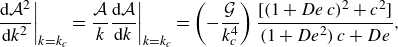 \begin{equation} \left .\frac {\textrm{d}\mathcal{A}^2}{\textrm{d} k^2}\right \vert _{k=k_c}=\left .\frac {\mathcal{A}}{k}\frac {\textrm{d}\mathcal{A}}{\textrm{d} k}\right \vert _{k=k_c}=\left (-\frac {\mathcal{G}}{k_c^4}\right )\frac {[(1+De\, c)^2+c^2]}{(1+De^2)\,c+De}, \end{equation}
and setting its reciprocal to zero, upon noting that $b=0$
and
$b=0$
and $c=-({2 }/{5})Re$
for
$c=-({2 }/{5})Re$
for $k=k_c$
. Observe that (5.1) is positive when the denominator is positive. This criterion is exactly satisfied when (4.4) is satisfied, for which monotonic Faraday instability occurs in the case of zero gravity.
$k=k_c$
. Observe that (5.1) is positive when the denominator is positive. This criterion is exactly satisfied when (4.4) is satisfied, for which monotonic Faraday instability occurs in the case of zero gravity.
Let us now consider how $f^*_{c1}$
changes with elasticity. To do this, we employ (4.7) and draw figure 8, which implicitly depicts the dependence of
$f^*_{c1}$
changes with elasticity. To do this, we employ (4.7) and draw figure 8, which implicitly depicts the dependence of $f^*_{c1}=\omega ^*_{c1}/2\pi$
on elasticity, i.e.
$f^*_{c1}=\omega ^*_{c1}/2\pi$
on elasticity, i.e. $1/G$
. The scaled frequency is expressed here as
$1/G$
. The scaled frequency is expressed here as $Re_{c1}=\omega ^*_{c1}\times (d^{*2}\rho /\mu )$
and the scaled elasticity is expressed as
$Re_{c1}=\omega ^*_{c1}\times (d^{*2}\rho /\mu )$
and the scaled elasticity is expressed as $De/Re=(1/G)\times (\mu ^2/d^{*2} \rho )$
, assuming
$De/Re=(1/G)\times (\mu ^2/d^{*2} \rho )$
, assuming $\rho, \mu$
and
$\rho, \mu$
and $d^*$
are held fixed. Equation (4.7) reveals that the lowest permissible value of
$d^*$
are held fixed. Equation (4.7) reveals that the lowest permissible value of $De/Re$
is
$De/Re$
is $2/5$
. We also see from (4.7) that
$2/5$
. We also see from (4.7) that $Re_{c1}$
increases to a maximum value of
$Re_{c1}$
increases to a maximum value of $5/4$
when
$5/4$
when $De/Re$
is
$De/Re$
is $4/5$
. This implies that at the maximum,
$4/5$
. This implies that at the maximum, $Re_{c1}\times (De/Re)=\omega ^*_{c1}\times (\mu /G)=1$
. That is, at the maximum, the critical frequency is equal to the inverse of the relaxation time. The decrease in
$Re_{c1}\times (De/Re)=\omega ^*_{c1}\times (\mu /G)=1$
. That is, at the maximum, the critical frequency is equal to the inverse of the relaxation time. The decrease in $Re_{c1}$
after the maximum is due to the inertial effects provided by elasticity. Further increase in
$Re_{c1}$
after the maximum is due to the inertial effects provided by elasticity. Further increase in $De/Re$
cause
$De/Re$
cause $Re_{c1}$
to approach zero as
$Re_{c1}$
to approach zero as $De/Re\to \infty$
.
$De/Re\to \infty$
.
Phase diagram depicting the first critical frequency, $f^*_{c1}=\omega ^*_{c1}/2\pi$
, expressed as
$f^*_{c1}=\omega ^*_{c1}/2\pi$
, expressed as $Re_{c1}$
versus
$Re_{c1}$
versus $De/Re$
, obtained from (4.7). The maximum critical frequency for a given
$De/Re$
, obtained from (4.7). The maximum critical frequency for a given $De/Re$
is denoted by
$De/Re$
is denoted by $\bullet$
.
$\bullet$
.
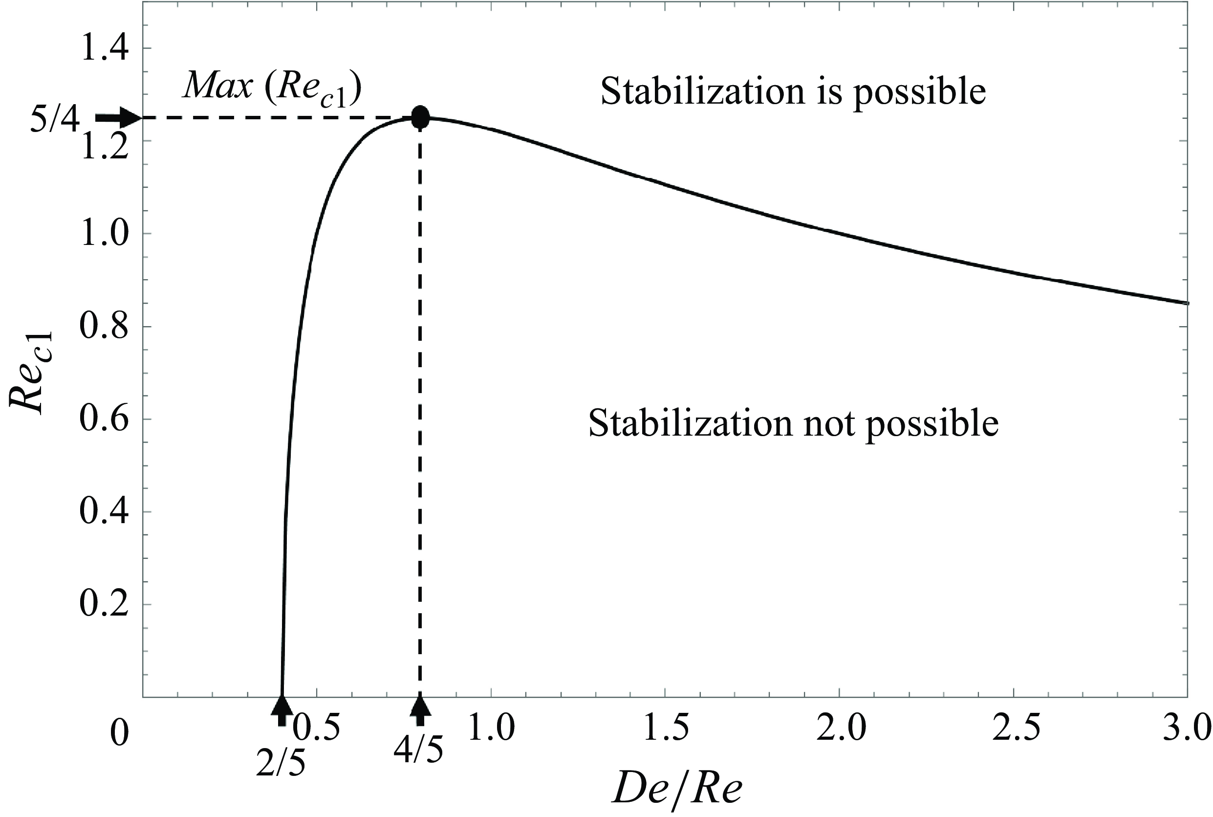
In summary, the first critical frequency approaches zero at the low end of $De/Re$
due to inertial action by momentum and at the high end of
$De/Re$
due to inertial action by momentum and at the high end of $De/Re$
due to elastic effects. As illustrated by the phase diagram, figure 8, parametric forcing cannot stabilize a gravitationally unstable system below the curve, whereas above the curve, parametric forcing can stabilize an otherwise gravitationally unstable system. This sets apart the behaviour of the viscoelastic case from the Newtonian case, for which the first critical frequency is completely absent. We now turn to the second critical frequency.
$De/Re$
due to elastic effects. As illustrated by the phase diagram, figure 8, parametric forcing cannot stabilize a gravitationally unstable system below the curve, whereas above the curve, parametric forcing can stabilize an otherwise gravitationally unstable system. This sets apart the behaviour of the viscoelastic case from the Newtonian case, for which the first critical frequency is completely absent. We now turn to the second critical frequency.
The second critical frequency, denoted $f^*_{c2}$
and marked by
$f^*_{c2}$
and marked by $\circ$
in figure 6(b) is defined as the frequency beyond which stabilization cannot be achieved. This frequency is greatly influenced not only by
$\circ$
in figure 6(b) is defined as the frequency beyond which stabilization cannot be achieved. This frequency is greatly influenced not only by $De/Re$
but also by the Bond number,
$De/Re$
but also by the Bond number, $B$
. Its origin can be determined by comparing the
$B$
. Its origin can be determined by comparing the $\mathcal{A}$
versus
$\mathcal{A}$
versus $k$
critical curves plotted for two frequencies on either side of
$k$
critical curves plotted for two frequencies on either side of $f^*_{c2}$
, say
$f^*_{c2}$
, say $f^*={2}{\,\rm Hz}$
and
$f^*={2}{\,\rm Hz}$
and $f^*={8}{\,\rm Hz}$
, marked by the vertical arrows in figure 6(b). As illustrated in figure 7(b) (at
$f^*={8}{\,\rm Hz}$
, marked by the vertical arrows in figure 6(b). As illustrated in figure 7(b) (at $f^*={2}{\,\rm Hz}$
), the threshold for stabilization of the monotonic mode,
$f^*={2}{\,\rm Hz}$
), the threshold for stabilization of the monotonic mode, $\mathcal{A}_s$
, marked by the open circle, has a lower value compared with the critical amplitude for the onset of the oscillatory instability,
$\mathcal{A}_s$
, marked by the open circle, has a lower value compared with the critical amplitude for the onset of the oscillatory instability, $\mathcal{A}_o$
, marked by the filled circle. By contrast, in figure 7(c) (at
$\mathcal{A}_o$
, marked by the filled circle. By contrast, in figure 7(c) (at $f^*={8}{\,\rm Hz}$
), we observe the opposite trend. Thus, there must be a critical frequency at which
$f^*={8}{\,\rm Hz}$
), we observe the opposite trend. Thus, there must be a critical frequency at which $\mathcal{A}_s$
equals
$\mathcal{A}_s$
equals $\mathcal{A}_o$
. Beyond this value, a resonant instability is observed and stabilization of a gravitationally unstable system can no longer be achieved.
$\mathcal{A}_o$
. Beyond this value, a resonant instability is observed and stabilization of a gravitationally unstable system can no longer be achieved.
Let us first consider how $f^*_{c2}$
changes with elasticity. Recall from § 3 that the damping rate increases with an increase in
$f^*_{c2}$
changes with elasticity. Recall from § 3 that the damping rate increases with an increase in $De$
in the low Deborah number regime (
$De$
in the low Deborah number regime ( $De/Re\lt 1/10$
, cf. figure 2
a), whereas it decreases with an increase in
$De/Re\lt 1/10$
, cf. figure 2
a), whereas it decreases with an increase in $De$
in the large Deborah number regime. This translates into an increase in
$De$
in the large Deborah number regime. This translates into an increase in $\mathcal{A}_o$
with increasing
$\mathcal{A}_o$
with increasing $De$
in the low
$De$
in the low $De$
region, therefore shifting
$De$
region, therefore shifting $f^*_{c2}$
to the right and vice versa in the large
$f^*_{c2}$
to the right and vice versa in the large $De$
region. We illustrate this change within the large
$De$
region. We illustrate this change within the large $De$
region using figure 9(a), where all parameters are the same as in figure 6, except for
$De$
region using figure 9(a), where all parameters are the same as in figure 6, except for $De/Re$
, which is now much lower, i.e.
$De/Re$
, which is now much lower, i.e. $De/Re=2/5$
. As a result
$De/Re=2/5$
. As a result $f^*_{c2}$
shifts to the right, and the region where stabilization can be achieved displays several islands of stability, due to the choppiness of the threshold,
$f^*_{c2}$
shifts to the right, and the region where stabilization can be achieved displays several islands of stability, due to the choppiness of the threshold, $\mathcal{A}_o$
, for the oscillatory mode. However, the bounds for the monotonic and oscillatory modes do not intersect in the low-frequency regime, as predicted by (4.7), which requires
$\mathcal{A}_o$
, for the oscillatory mode. However, the bounds for the monotonic and oscillatory modes do not intersect in the low-frequency regime, as predicted by (4.7), which requires $De/Re\gt 2/5$
for the existence of
$De/Re\gt 2/5$
for the existence of $f^*_{c_1}$
. Thus, there is only one critical frequency, i.e.
$f^*_{c_1}$
. Thus, there is only one critical frequency, i.e. $f^*_{c2}$
.
$f^*_{c2}$
.
Another interesting limit to consider is where the stabilization region in figure 6(b) disappears entirely. This is shown in figure 9(b), where all parameters are the same as in figure 6, except for $B$
, which is now higher, i.e.
$B$
, which is now higher, i.e. $B=0.32$
. An increase in Bond number,
$B=0.32$
. An increase in Bond number, $B$
, i.e. an increase in gravitational acceleration, necessitates higher values of forcing amplitudes,
$B$
, i.e. an increase in gravitational acceleration, necessitates higher values of forcing amplitudes, $\mathcal{A}_s$
, for complete stabilization. However, it does not significantly change
$\mathcal{A}_s$
, for complete stabilization. However, it does not significantly change $\mathcal{A}_o$
. Consequently, the value of
$\mathcal{A}_o$
. Consequently, the value of $f^*_{c2}$
decreases and the region of stability in figure 6(b) shrinks. At a certain Bond number value, the first and the second critical frequencies coincide, i.e.
$f^*_{c2}$
decreases and the region of stability in figure 6(b) shrinks. At a certain Bond number value, the first and the second critical frequencies coincide, i.e. $f^*_{c1}=f^*_{c2}$
, and stabilization via parametric forcing can no longer be achieved. For the viscoelastic fluid under consideration in figures 6(b) and 9(b), this value is
$f^*_{c1}=f^*_{c2}$
, and stabilization via parametric forcing can no longer be achieved. For the viscoelastic fluid under consideration in figures 6(b) and 9(b), this value is $B=0.32$
.
$B=0.32$
.
In summary, while moving from figure 6(b) to figures 9(a) and 9(b), we observe either two, one, or zero critical frequencies, i.e, the stabilization region is bounded either on both sides, on one side or is simply non-existent.
Stability bounds using the same properties as in figure 6 except for different values of $De/Re$
and
$De/Re$
and $B$
. (a) Single critical frequency for
$B$
. (a) Single critical frequency for $B=0.1$
and
$B=0.1$
and $De/Re=2/5$
; (b) coinciding critical frequencies for
$De/Re=2/5$
; (b) coinciding critical frequencies for $B=0.32$
and
$B=0.32$
and $De/Re=2$
. The
$De/Re=2$
. The $\star$
marks
$\star$
marks $f^*_{c1}=f^*_{c2}$
.
$f^*_{c1}=f^*_{c2}$
.
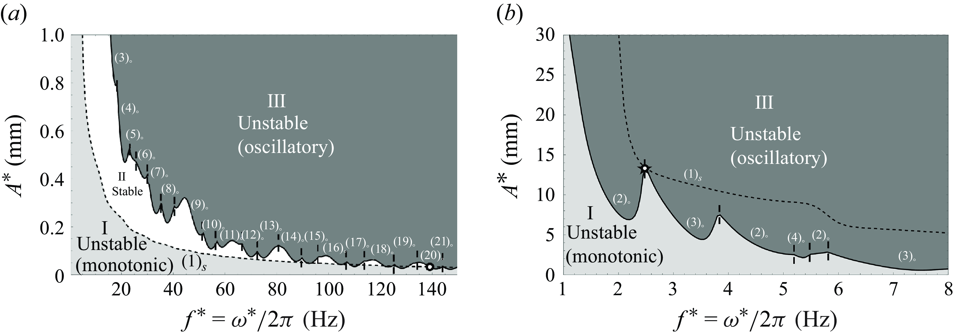
6. Summary
In this work, the stability characteristics of a viscoelastic fluid layer undergoing parametric forcing in both gravitationally stable ( $\mathbf{g}\gt \mathbf{0}$
) and unstable (
$\mathbf{g}\gt \mathbf{0}$
) and unstable ( $\mathbf{g}\lt \mathbf{0}$
) configurations have been investigated by calculations that are supported by analytical expressions. The inverse time constants,
$\mathbf{g}\lt \mathbf{0}$
) configurations have been investigated by calculations that are supported by analytical expressions. The inverse time constants, $\sigma$
, obtained in the absence of forcing for
$\sigma$
, obtained in the absence of forcing for $\mathbf{g}\gt 0$
are used to gain insight into the threshold amplitudes and the temporal response of the Faraday instability. In particular, we track how the real part of the leading
$\mathbf{g}\gt 0$
are used to gain insight into the threshold amplitudes and the temporal response of the Faraday instability. In particular, we track how the real part of the leading $\sigma$
, i.e. the damping rate, changes with elasticity. For weakly elastic fluids, we find that increased elasticity increases the damping rate, thereby raising the Faraday instability threshold. By contrast, for dominantly elastic fluids, the damping rate is reduced with increasing elasticity, thus decreasing the threshold.
$\sigma$
, i.e. the damping rate, changes with elasticity. For weakly elastic fluids, we find that increased elasticity increases the damping rate, thereby raising the Faraday instability threshold. By contrast, for dominantly elastic fluids, the damping rate is reduced with increasing elasticity, thus decreasing the threshold.
The imaginary part of the inverse time constants informs us about the temporal response of the interface to Faraday instability. We find the possibility of both purely real $\sigma$
, as well as complex
$\sigma$
, as well as complex $\sigma$
, thereby introducing the possibility of both monotonic and oscillatory responses upon instability. We show further that the nature of the response upon parametric forcing is highly dependent on the direction and the magnitude of gravitational acceleration,
$\sigma$
, thereby introducing the possibility of both monotonic and oscillatory responses upon instability. We show further that the nature of the response upon parametric forcing is highly dependent on the direction and the magnitude of gravitational acceleration, $\mathbf{g}$
.
$\mathbf{g}$
.
If $\mathbf{g}\gt 0$
, an oscillatory response is seen upon resonance, when
$\mathbf{g}\gt 0$
, an oscillatory response is seen upon resonance, when $\vert \mathbf{g}\vert$
is of the order of Earth’s gravity. However, at low
$\vert \mathbf{g}\vert$
is of the order of Earth’s gravity. However, at low $\mathbf{g}$
and in microgravity (
$\mathbf{g}$
and in microgravity ( $\mathbf{g}\sim \mathbf{0}$
), a dominantly monotonic response will arise, if the momentum-induced inertia is weak compared with elastic effects. For a given viscoelastic fluid, this new type of instability is observed until a critical frequency, beyond which the momentum-induced inertia of the fluid dominates, leading to an oscillatory response. By contrast, in Newtonian liquids, an oscillatory instability is observed at all gravity levels.
$\mathbf{g}\sim \mathbf{0}$
), a dominantly monotonic response will arise, if the momentum-induced inertia is weak compared with elastic effects. For a given viscoelastic fluid, this new type of instability is observed until a critical frequency, beyond which the momentum-induced inertia of the fluid dominates, leading to an oscillatory response. By contrast, in Newtonian liquids, an oscillatory instability is observed at all gravity levels.
If $\mathbf{g}\lt \mathbf{0}$
, the stabilizing or destabilizing influence provided by parametric forcing changes with the fluid’s elasticity. We find that a stable quiescent state is achievable when forced within a finite amplitude range between two critical frequencies. For amplitudes below this range, a monotonic response is observed due to a Rayleigh–Taylor instability mechanism. For amplitudes above this range, an oscillatory response is observed on account of a Faraday instability mechanism. The quiescent stable region disappears if the frequency is either decreased below the first critical frequency or increased beyond the second critical frequency.
$\mathbf{g}\lt \mathbf{0}$
, the stabilizing or destabilizing influence provided by parametric forcing changes with the fluid’s elasticity. We find that a stable quiescent state is achievable when forced within a finite amplitude range between two critical frequencies. For amplitudes below this range, a monotonic response is observed due to a Rayleigh–Taylor instability mechanism. For amplitudes above this range, an oscillatory response is observed on account of a Faraday instability mechanism. The quiescent stable region disappears if the frequency is either decreased below the first critical frequency or increased beyond the second critical frequency.
The first critical frequency depends on both the fluid’s elasticity and viscosity, characterized by $De/Re$
. The value of the second critical frequency is additionally dependent on the magnitude of the gravitational acceleration,
$De/Re$
. The value of the second critical frequency is additionally dependent on the magnitude of the gravitational acceleration, $\mathbf{g}$
, characterized by the Bond number,
$\mathbf{g}$
, characterized by the Bond number, $B$
. At frequencies below the first critical frequency, parametric forcing promotes monotonic growth of the interface due to the weak influence of fluid inertia. However, at frequencies greater than the second critical frequency, inertia dominates, causing the system to exhibit oscillatory instability before stabilization can be possibly achieved. Consequently, outside the range bounded by the two critical values, the fluid is always unstable, with the system directly transitioning from monotonic to oscillatory instability. The stabilization region is the largest for weakly elastic fluids, for which the first critical frequency goes to zero and the second critical frequency increases significantly due to a higher Faraday threshold. Conversely, for strongly elastic fluids, the stabilization region decreases and then entirely disappears for a large enough Bond number.
$B$
. At frequencies below the first critical frequency, parametric forcing promotes monotonic growth of the interface due to the weak influence of fluid inertia. However, at frequencies greater than the second critical frequency, inertia dominates, causing the system to exhibit oscillatory instability before stabilization can be possibly achieved. Consequently, outside the range bounded by the two critical values, the fluid is always unstable, with the system directly transitioning from monotonic to oscillatory instability. The stabilization region is the largest for weakly elastic fluids, for which the first critical frequency goes to zero and the second critical frequency increases significantly due to a higher Faraday threshold. Conversely, for strongly elastic fluids, the stabilization region decreases and then entirely disappears for a large enough Bond number.
Thus, we find for viscoelastic fluids that the number of critical frequencies are two, one or none. This stands in stark contrast with the case of Newtonian fluids, where the region of stabilization is always bounded by a single critical frequency. It might be noted that complete stabilization is possible because the parametric forcing is normal to an erstwhile flat interface in the fluid’s base state. On the other hand, if other directions of parametric forcing are considered, the base state will necessarily involve sloshing and a non-flat interface in containers of finite horizontal extent as opposed to unbounded containers, cf. Or (Reference Or1997). Therefore, complete stabilization to a quiescent state would not be possible in bounded containers with horizontal forcing (Wolf Reference Wolf1969; Shevtsova et al. Reference Shevtsova, Gaponenko, Yasnou, Mialdun and Nepomnyashchy2016; Garcia-Gonzalez Reference Garcia-Gonzalez and Fernandez-Feria2017; Gligor et al. Reference Gligor, Sánchez, Porter and Shevtsova2020; Piao & Juel Reference Piao and Juel2025). Notwithstanding a non-trivial base state, future studies ought to consider other directions of parametric forcing due to their interesting physics (Piao & Juel Reference Piao and Juel2025).
The work in this study has used an upper convected Maxwell fluid as an example of a viscoelastic fluid. As there are several examples of Rayleigh–Taylor instability with soft solids (Mora et al. Reference Mora, Phou, Fromental and Pomeau2014; Riccobelli & Ciarletta Reference Riccobelli and Ciarletta2017; Tamim & Bostwick Reference Tamim and Bostwick2020; Dinesh & Narayanan Reference Dinesh and Narayanan2021; Slutzky et al. Reference Slutzky, Hwang, Stone and Nunes2023), studies on the effect of $\mathcal{G}$
on parametric forcing of other types of fluids and soft solids could be future avenues of research.
$\mathcal{G}$
on parametric forcing of other types of fluids and soft solids could be future avenues of research.
Funding
The authors gratefully acknowledge funding from National Science Foundation (R.N., grant numbers 2025117, 2422919) and NASA (R.N., grant numbers NNX17AL27G, 80NSSC23K0457). I.B.I. acknowledges support from a Chateaubriand fellowship.
Declaration of interests
The authors report no conflict of interest.
Appendix A. Derivation of the linear WRIBL model from § 2.3 and the algebraic expressions in table 1 and §§ 4.2 and 4.3.
In this appendix, we derive the linear long-wave model introduced in § 2.3, which is based on the WRIBL (weighted residual integral boundary layer) approach (Ruyer-Quil & Manneville Reference Ruyer-Quil and Manneville2000), and which we have used to obtain the algebraic expressions for the inverse time constants in table 1 and the expressions for neutral stability bounds in §§ 4.2 and 4.3.
Long-wave approximation
We commence by invoking the long-wave approximation, i.e. $\epsilon {\ll }1$
, where
$\epsilon {\ll }1$
, where $\epsilon$
=
$\epsilon$
= $d^*$
/
$d^*$
/ $W^*$
is the length scale ratio according to the scaling introduced in (2.8). Then, truncating the linearized governing equations (2.17)–(2.23) at
$W^*$
is the length scale ratio according to the scaling introduced in (2.8). Then, truncating the linearized governing equations (2.17)–(2.23) at $O(\epsilon )$
, we obtain the continuity equation
$O(\epsilon )$
, we obtain the continuity equation
 \begin{equation} k u+\frac {\partial w}{\partial z} = 0, \end{equation}
and the momentum equations
 \begin{equation} \epsilon Re \Bigl (\sigma + \frac {i n \omega }{2}\Bigr ) u = \epsilon k p +\frac {\partial \tau _{xz}}{\partial z} \end{equation}
and
 \begin{equation} - \epsilon \, \frac {\partial p}{\partial z}=0, \end{equation}
where we have assumed $Re$
to be at least
$Re$
to be at least $O(1)$
. Inertia, which plays an important role in Faraday instability, is retained as it enters at
$O(1)$
. Inertia, which plays an important role in Faraday instability, is retained as it enters at $O(\epsilon )$
in (A2). Applying the same procedure to the relevant component of the constitutive equations for the polymeric stresses (2.19), we obtain
$O(\epsilon )$
in (A2). Applying the same procedure to the relevant component of the constitutive equations for the polymeric stresses (2.19), we obtain
 \begin{equation} \Bigl (1+ De\Bigl (\sigma + \frac {i n \omega }{2}\Bigr ) \Bigr )\tau _{xz}= \frac {\partial u}{\partial z}, \end{equation}
where we have assumed $De$
to be at least
$De$
to be at least $O(\epsilon )$
.
$O(\epsilon )$
.
The boundary conditions at the bottom wall (2.20), $z=-1$
, become
$z=-1$
, become
 \begin{equation} u=0\,\,\mbox{and}\, \,w=0, \end{equation}
and the interphase coupling conditions, (2.21)–(2.23), at $z=0$
become
$z=0$
become
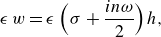 \begin{gather} \epsilon \,w= \epsilon \,\Bigl (\sigma + \frac {i n \omega }{2}\Bigr ) h, \end{gather}
 \begin{gather} \tau _{xz} =0,\text{ i.e., } \frac {\partial u} {\partial z} =0 \end{gather}
 \begin{gather} \text{and}\,\,\,\, \sum _{n=-N}^{n=N} e^{(in\omega t)/2}\epsilon \,\widehat {p}_n=\sum _{n=-N}^{n=N} e^{(in\omega t)/2}\left \{\epsilon (\mathcal{G} +\mathcal{A} cos(\omega t)) \widehat {h}_n+\frac {\epsilon ^{3}}{Ca} k^2 \widehat {h}_n\right \}, \end{gather}
where we have assumed $\mathcal{G}$
and
$\mathcal{G}$
and $\mathcal{A}$
to be at least
$\mathcal{A}$
to be at least $O(1)$
and
$O(1)$
and $Ca$
to be at least
$Ca$
to be at least $O(\epsilon ^2)$
. We remind the reader that (A1)–(A6b
) imply summation over all the temporal modes introduced in (2.14) and (2.15), which we had omitted in the writing of (2.17)–(2.22), for convenience.
$O(\epsilon ^2)$
. We remind the reader that (A1)–(A6b
) imply summation over all the temporal modes introduced in (2.14) and (2.15), which we had omitted in the writing of (2.17)–(2.22), for convenience.
From (A3), we see that $p$
is independent of
$p$
is independent of $z$
. Therefore,
$z$
. Therefore, $p$
is fully defined by (A6c
), which is then substituted into (A2), resulting in
$p$
is fully defined by (A6c
), which is then substituted into (A2), resulting in
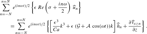 \begin{align} & \sum _{n=-N}^{n=N} e^{(in\omega t)/2}\left \{ \epsilon \,Re \left (\sigma + \frac {i n \omega }{2}\right ) \, \widehat {u}_n\right \}\notag \\&\qquad = \sum _{n=-N}^{n=N} e^{(in\omega t)/2}\left \{\left [\frac {\epsilon ^{3}}{Ca} k^3 +\epsilon \,(\mathcal{G}+\mathcal{A}\,\cos(\omega t)) k \right ]\widehat {h}_n+\frac {\partial \widehat {\tau }_{xz\,n}}{\partial z}\right \}. \end{align}
Finally, (A7) is inserted into (A4), to obtain
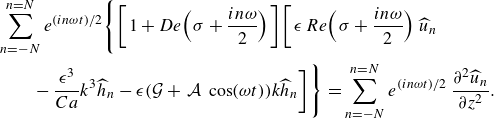 \begin{equation} \begin{aligned} &\sum _{n=-N}^{n=N} e^{(in\omega t)/2}\Bigg \{\bigg [1+De\Bigl (\sigma + \frac {i n \omega }{2}\Bigr ) \bigg ]\bigg [\epsilon \, Re\Bigl (\sigma + \frac {i n \omega }{2}\Bigr ) \, \widehat {u}_n \\ & \qquad -\frac {\epsilon ^{3}}{Ca} k^3 \widehat {h}_n-\epsilon (\mathcal{G}+\,\mathcal{A}\,\cos(\omega t)) k \widehat {h}_n\bigg ]\Bigg \} = \sum _{n=-N}^{n=N} e^{(in\omega t)/2}\,\frac {\partial ^2 \widehat {u}_n}{\partial z^2}. \end{aligned} \end{equation}
Equation (A8) may be solved for $\widehat {u}_n(z)$
subject to (A5) and (A6b
). Inserting this solution into (A1) and integrating the latter from
$\widehat {u}_n(z)$
subject to (A5) and (A6b
). Inserting this solution into (A1) and integrating the latter from $z=-1$
to
$z=-1$
to $z=0$
, while invoking (A5) and (A6a
), yields a characteristic equation for the eigenvalue,
$z=0$
, while invoking (A5) and (A6a
), yields a characteristic equation for the eigenvalue, $\sigma$
. This equation may be viewed from two perspectives. In the first perspective,
$\sigma$
. This equation may be viewed from two perspectives. In the first perspective, $\mathcal{A}$
is set to zero, which implies
$\mathcal{A}$
is set to zero, which implies $N=0$
, yielding a transcendental algebraic equation for
$N=0$
, yielding a transcendental algebraic equation for $\sigma (k^2)$
, which must be solved numerically for the roots. In the second perspective,
$\sigma (k^2)$
, which must be solved numerically for the roots. In the second perspective, $\sigma$
is set to zero and an equation of the form (2.24) is obtained, which must be solved numerically for
$\sigma$
is set to zero and an equation of the form (2.24) is obtained, which must be solved numerically for $\mathcal{A}$
, yielding the critical forcing amplitude.
$\mathcal{A}$
, yielding the critical forcing amplitude.
However, by applying the WRIBL approach to the linearized equations, (A1) and (A8), an approximate characteristic equation for $\sigma$
can be obtained, which is analytically tractable in certain limits. This is due to the integral nature of the WRIBL approach, which dispenses with needing to solve for the eigenfunctions,
$\sigma$
can be obtained, which is analytically tractable in certain limits. This is due to the integral nature of the WRIBL approach, which dispenses with needing to solve for the eigenfunctions, $\widehat {u}_n(z)$
,
$\widehat {u}_n(z)$
, $\widehat {w}_n(z)$
and
$\widehat {w}_n(z)$
and $\widehat {p}_n$
. In particular, we will obtain analytical expressions for (i)
$\widehat {p}_n$
. In particular, we will obtain analytical expressions for (i) $\sigma$
in terms of
$\sigma$
in terms of $k$
in the Newtonian limit and
$k$
in the Newtonian limit and $\mathcal{A}$
= 0 and (ii) the critical
$\mathcal{A}$
= 0 and (ii) the critical $\mathcal{A}$
in terms of
$\mathcal{A}$
in terms of $k$
for a viscoelastic fluid. Capturing the dependency on
$k$
for a viscoelastic fluid. Capturing the dependency on $k$
, turns out to be crucial in our current system.
$k$
, turns out to be crucial in our current system.
The WRIBL model
We reduce the dimension of the system of governing equations (A1) and (A8) by eliminating all spatial dependence and describing the flow in terms of the flow rate, $q$
, and interface deflection,
$q$
, and interface deflection, $h$
. This is achieved by integrating (A1) and (A8) across the film thickness, i.e. from
$h$
. This is achieved by integrating (A1) and (A8) across the film thickness, i.e. from $z=-1$
to
$z=-1$
to $z=0$
. To this end, we integrate the continuity equation (A1) and invoke (A6a
). This yields
$z=0$
. To this end, we integrate the continuity equation (A1) and invoke (A6a
). This yields
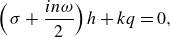 \begin{equation} \Bigl (\sigma + \frac {i n \omega }{2}\Bigr ) h + k q=0, \end{equation}
where $q=\int _{-1}^{0} u\,\textrm{d}z$
.
$q=\int _{-1}^{0} u\,\textrm{d}z$
.
We next obtain an integrated form of the integral momentum equation. To do this we first decompose the dependent variable, $u$
, into a leading-order contribution (denoted by a tilde) and an
$u$
, into a leading-order contribution (denoted by a tilde) and an $O(\epsilon )$
correction (denoted by a prime), i.e.
$O(\epsilon )$
correction (denoted by a prime), i.e.
 \begin{equation} u(z)=\underbrace {\widetilde {u}(z)}_{O(1)}+\underbrace {{u^{\prime}}(z)}_{O(\epsilon )}. \end{equation}
The leading-order velocity, $\widetilde {u}$
, is obtained by truncating (A1)–(A8) at
$\widetilde {u}$
, is obtained by truncating (A1)–(A8) at $O(1)$
, restricting
$O(1)$
, restricting $Ca$
to be at most of order
$Ca$
to be at most of order $O(\epsilon ^{3})$
.
$O(\epsilon ^{3})$
.
The boundary value problem, governing $\widetilde {u}$
is
$\widetilde {u}$
is
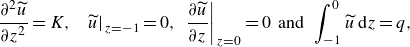 \begin{equation} \begin{aligned} \frac {\partial ^{2}\widetilde {u}}{\partial z^{2}}=K,\,\,\,\, \widetilde {u}\big \vert _{z=-1}=0,\,\,\frac {\partial \widetilde {u}}{\partial z}\bigg \vert _{z=0}=0\,\,\mbox{and}\,\,\int _{-1}^{0} \widetilde {u} \,\textrm{d}z=q, \end{aligned} \end{equation}
where $K$
is a constant.
$K$
is a constant.
Solving (A11), yields
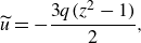 \begin{equation} \widetilde {u}=-\frac {3 q (z^2-1)}{2}, \end{equation}
which implies for the velocity correction, $u^{\prime}$
,
$u^{\prime}$
,
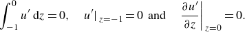 \begin{equation} \int _{-1}^{0} u^{\prime} \,\textrm{d}z=0,\quad {u^{\prime}}\big \vert _{z=-1}=0\,\,\text{and}\,\quad \frac {\partial {u^{\prime}}}{\partial z}\bigg \vert _{z=0}=0. \end{equation}
We next introduce (A10), (A12) and (A13) in (A8), truncate the resulting equations at $O(\epsilon )$
, multiply by a weight function
$O(\epsilon )$
, multiply by a weight function $F(z)$
to be determined later, and integrate across the film height, obtaining
$F(z)$
to be determined later, and integrate across the film height, obtaining

where the boxed terms in (A14) can be rewritten, upon integration by parts, as
 \begin{equation} \begin{aligned} \int _{-1}^{0} \frac {\partial ^{2} }{\partial z^{2}}(\widehat {\widetilde {u}}_n+ \widehat {u^{\prime}}_n) F\,\textrm{d}z=\left [\frac {\partial (\widehat {\widetilde {u}}_n+ \widehat {u^{\prime}}_n) }{\partial z} F-(\widehat {\widetilde {u}}_n+ \widehat {u^{\prime}}_n)\,\frac {\partial F}{\partial z} \right ]_{-1}^{0}+\int _{-1}^{0} (\widehat {\widetilde {u}}_n+ \widehat {u^{\prime}}_n) \,\textrm{d}z. \end{aligned} \end{equation}
The weight function, $F(z)$
, is a polynomial obtained by solving an equation similar to that of the leading-order velocity
$F(z)$
, is a polynomial obtained by solving an equation similar to that of the leading-order velocity $\widehat {\widetilde {u}}_n$
(A11). This weighted integration also called the Galerkin projection will cancel all of the
$\widehat {\widetilde {u}}_n$
(A11). This weighted integration also called the Galerkin projection will cancel all of the $\widehat {u^{\prime}}_n$
terms, which are unknown in (A15). The governing equations for
$\widehat {u^{\prime}}_n$
terms, which are unknown in (A15). The governing equations for $F$
are
$F$
are
 \begin{equation} \begin{aligned} \frac {\partial ^{2}F}{\partial z^{2}}=1,\quad F\big \vert _{z=-1}=0\,\,\text{and}\quad \frac {\partial F}{\partial z}\bigg \vert _{z=0}=0, \end{aligned} \end{equation}
yielding
 \begin{equation} F=\frac {1}{2} (z^2-1). \end{equation}
This results in the following form of the integrated momentum equation:
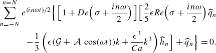 \begin{equation} \begin{aligned} \sum _{n=-N}^{n=N} e^{(in\omega t)/2}\Bigl \{\Bigl [1+De\Bigl (\sigma + \frac {i n \omega }{2}\Bigr ) \Bigr ]\Bigl [\frac {2}{5} \epsilon \textit {Re} \Bigl (\sigma + \frac {i n \omega }{2}\Bigr ) \widehat {q}_n\\-\frac {1}{3}\left (\epsilon (\mathcal{G}+\,\mathcal{A}\,\cos(\omega t)) k +\frac {\epsilon ^{3}}{Ca} k^3 \right )\widehat {h}_n\Bigr ]+\widehat {q}_n\Bigr \}=0. \end{aligned} \end{equation}
To make the equations applicable when we consider disturbances of arbitrary wavenumbers, we rescale the equations by using a common length scale, $d^*$
, and time scale,
$d^*$
, and time scale, $d^*/U$
. This results in
$d^*/U$
. This results in $\sigma \to \sigma /\epsilon$
,
$\sigma \to \sigma /\epsilon$
, $\omega \to \omega /\epsilon$
,
$\omega \to \omega /\epsilon$
, $k\to k \epsilon$
,
$k\to k \epsilon$
, $De\to \epsilon De$
. The resulting equation takes the form
$De\to \epsilon De$
. The resulting equation takes the form
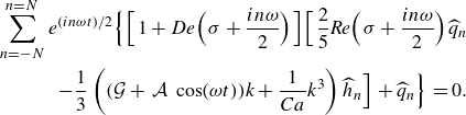 \begin{equation} \begin{aligned} \sum _{n=-N}^{n=N} e^{(in\omega t)/2}\Bigl \{\Bigl [1+De\Bigl (\sigma + \frac {i n \omega }{2}\Bigr ) \Bigr ]\Bigl [\frac {2}{5} \textit {Re} \Bigl (\sigma + \frac {i n \omega }{2}\Bigr ) \widehat {q}_n\\-\frac {1}{3}\left ((\mathcal{G}+\,\mathcal{A}\,\cos(\omega t)) k +\frac {1}{Ca} k^3 \right )\widehat {h}_n\Bigr ]+\widehat {q}_n\Bigr \}=0. \end{aligned} \end{equation}
Substituting $q$
from the integrated continuity equation (A9) into (A19), yields
$q$
from the integrated continuity equation (A9) into (A19), yields
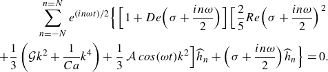 \begin{equation} \begin{aligned} \sum _{n=-N}^{n=N} e^{(in\omega t)/2}\Bigl \{\Bigl [1+De\Bigl (\sigma +\frac {i n \omega }{2}\Bigr ) \Bigr ]\Bigl [\frac {2}{5} Re\Bigl (\sigma + \frac {i n \omega }{2}\Bigr )^2 \, \\+\frac {1}{3}\left (\mathcal{G} k^2 + \frac {1}{Ca} k^4 \right )+\frac {1}{3}\,\mathcal{A}\,cos(\omega t)k^2 \Bigr ]\widehat {h}_n+\Bigl (\sigma + \frac {i n \omega }{2}\Bigr )\widehat {h}_n\Bigl \}=0. \end{aligned} \end{equation}
which is the same as (2.25).
Characteristic equation for inverse time constant,
$\sigma$

To determine the inverse time constants, we set $\mathcal{A}=0$
and
$\mathcal{A}=0$
and $\omega =0$
in (A20) and divide the result by
$\omega =0$
in (A20) and divide the result by $a$
, yielding a characteristic equation for
$a$
, yielding a characteristic equation for $\sigma /a$
, viz.
$\sigma /a$
, viz.
 \begin{equation} (a De) \, \Bigl (\frac {\sigma }{a}\Bigr )^3+\Bigl (\frac {\sigma }{a}\Bigr )^2 + \, \left(1+\left[\frac {b}{a}\right](a De)\right)\left(\frac {\sigma }{a}\right)+\left[\frac {b}{a}\right]=0, \end{equation}
a group that is independent of the characteristic time scale, where $a={5}/({2 Re})$
depends on the viscosity,
$a={5}/({2 Re})$
depends on the viscosity, $\nu$
, and
$\nu$
, and $b=({1}/{3}) ({k^4}/{Ca}+k^2\mathcal{G} )$
depends on the wavenumber,
$b=({1}/{3}) ({k^4}/{Ca}+k^2\mathcal{G} )$
depends on the wavenumber, $k$
. Equation (A21) is the same as (2.26).
$k$
. Equation (A21) is the same as (2.26).
Although these $\sigma$
can be determined numerically from (A21), we shall be interested in the limit
$\sigma$
can be determined numerically from (A21), we shall be interested in the limit $k\to 0$
. Algebraic expressions for the
$k\to 0$
. Algebraic expressions for the $\sigma$
can then be obtained. This task is enabled by considering the fluid to be of infinite horizontal extent, upon which the unknown dependent variables,
$\sigma$
can then be obtained. This task is enabled by considering the fluid to be of infinite horizontal extent, upon which the unknown dependent variables, $\psi$
, are now expressed as
$\psi$
, are now expressed as $\psi =\psi _0+\psi _1 e^{ikx}e^{\sigma t}$
, now taking
$\psi =\psi _0+\psi _1 e^{ikx}e^{\sigma t}$
, now taking $k$
to be continuous. This results in the characteristic equation:
$k$
to be continuous. This results in the characteristic equation:
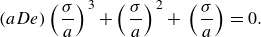 \begin{equation} (a De) \, \Bigl (\frac {\sigma }{a}\Bigr )^3+\Bigl (\frac {\sigma }{a}\Bigr )^2 + \, \Bigl (\frac {\sigma }{a}\Bigr )=0. \end{equation}
To obtain these forms, $\epsilon$
must now be
$\epsilon$
must now be $d^*/\Lambda ^*$
in the scaled forms given in (2.8), where
$d^*/\Lambda ^*$
in the scaled forms given in (2.8), where $\Lambda ^*$
is the characteristic wavelength. The cubic equation (A22) yields three roots for
$\Lambda ^*$
is the characteristic wavelength. The cubic equation (A22) yields three roots for $\sigma$
, with one of the roots being zero. Equation (A22) may be examined in the limit of low
$\sigma$
, with one of the roots being zero. Equation (A22) may be examined in the limit of low $De$
and high
$De$
and high $De$
.
$De$
.
(i) Small $\mathbf{De}$
. For small values of
$\mathbf{De}$
. For small values of $De$
, a singular perturbation expansion in
$De$
, a singular perturbation expansion in $(a De)$
given by
$(a De)$
given by
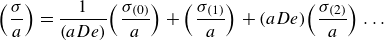 \begin{equation} \Bigl (\frac {\sigma }{a}\Bigr )=\frac {1}{(a De)}\Bigl (\frac {\sigma _{(0)}}{a}\Bigr )+\Bigl (\frac {\sigma _{(1)}}{a}\Bigr )+ (a De)\Bigl (\frac {\sigma _{(2)}}{a}\Bigr )\ldots \end{equation}
is employed to solve (A22). Upon substitution of the expansion, the resulting equations are solved for different powers of $(aDe)$
. The roots thus obtained are
$(aDe)$
. The roots thus obtained are
 \begin{equation} \frac {\sigma _1}{a}=0,\,\frac {\sigma _2}{a}=-1-a De+O(a De)^2,\text{ and}\,\frac {\sigma _3}{a}=-\frac {1}{a De }+1+a De+O(a De)^2. \end{equation}
(ii) Large $\mathbf{De}$
. At large values of
$\mathbf{De}$
. At large values of $De$
, since one of the roots is known to be zero, the other two roots can be found from the resulting quadratic equation. The roots obtained using (A22) are
$De$
, since one of the roots is known to be zero, the other two roots can be found from the resulting quadratic equation. The roots obtained using (A22) are
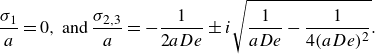 \begin{equation} \frac {\sigma _1}{a}=0,\,\text{and}\,\frac {\sigma _{2,3}}{a}=-\frac {1}{2a De }\pm i\sqrt {\frac {1}{a De }-\frac {1}{4(aDe)^2 }}. \end{equation}
These results for the inverse time constants are presented in table 1.
Analytical expression for critical amplitude,
$\mathcal{A}$

The critical amplitude for predicting the onset of monotonic instability due to parametric forcing can be calculated by setting $\sigma =0$
and performing the Floquet summation for
$\sigma =0$
and performing the Floquet summation for $n=-2,0$
and
$n=-2,0$
and $2$
, i.e. thereby considering only the monotonic and lowest harmonic modes. This yields an eigenvalue problem of the form
$2$
, i.e. thereby considering only the monotonic and lowest harmonic modes. This yields an eigenvalue problem of the form
 \begin{equation} \mathbf{Cx}=\mathcal{A}\,\mathbf{Dx}, \end{equation}
with eigenvalue, $\mathcal{A}$
, and eigenvectors
$\mathcal{A}$
, and eigenvectors $\mathbf{x}=\{\widehat {h}_2,\widehat {h}_{0},\widehat {h}_{-2}\}$
. The Det[
$\mathbf{x}=\{\widehat {h}_2,\widehat {h}_{0},\widehat {h}_{-2}\}$
. The Det[ ${\mathbf{C}-\mathcal{A}D}$
] must be zero for non-trivial solutions, yielding the square of the critical amplitude as
${\mathbf{C}-\mathcal{A}D}$
] must be zero for non-trivial solutions, yielding the square of the critical amplitude as
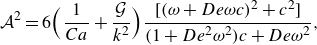 \begin{equation} \mathcal{A}^2=6\Bigl (\frac {1}{Ca}+\frac {\mathcal{G}}{k^2 }\Bigr )\frac {[(\omega +De\omega c)^2+c^2]}{(1+De^2\omega ^2)c+De\omega ^2}, \end{equation}
where $c=b-\frac {\omega ^2}{a}$
. Note that the frequency is scaled with respect to
$c=b-\frac {\omega ^2}{a}$
. Note that the frequency is scaled with respect to $\omega ^*$
, the parametric frequency, thereby rendering
$\omega ^*$
, the parametric frequency, thereby rendering $\omega =1$
. The extent of the monotonic nature of the interface response can be determined from the ratio
$\omega =1$
. The extent of the monotonic nature of the interface response can be determined from the ratio
 \begin{equation} \frac {\widehat {h}_o}{\widehat {h}_2+\widehat {h}_{-2}}=\frac {\mathcal{A}}{2\left (\frac {k^2}{Ca}+\mathcal{G}\right )}. \end{equation}
Here $\mathcal{A}$
versus
$\mathcal{A}$
versus $k$
curves. Comparison of threshold obtained using the algebraic expression (A26) (dashed curve) and the numerical results obtained using the full equations (solid curves).
$k$
curves. Comparison of threshold obtained using the algebraic expression (A26) (dashed curve) and the numerical results obtained using the full equations (solid curves).
The algebraic expression (A26), which is the same as (2.28), accurately predicts the critical amplitude at low wavenumbers and when the instability response is monotonically dominant. This is illustrated in figure 10, where this expression, depicted by a dashed curve, is compared with the numerical results obtained using the full-governing equations shown in figure 4(a).
Criteria for the existence of a purely monotonic response
We observe from expressions given in (A26) and (A27) that, when $\mathcal{G}\to 0$
and
$\mathcal{G}\to 0$
and $k\to 0$
, we have a purely monotonic instability for
$k\to 0$
, we have a purely monotonic instability for $\mathcal{A}^2\geqslant 0$
. To see this, we set
$\mathcal{A}^2\geqslant 0$
. To see this, we set $\mathcal{G}=0$
and
$\mathcal{G}=0$
and $k=0$
and determine the parameters for which the expression in (A26) yields a positive value. Equation (A26) becomes
$k=0$
and determine the parameters for which the expression in (A26) yields a positive value. Equation (A26) becomes
 \begin{equation} \mathcal{A}^2=\frac {6}{Ca}\frac {[(1-(\frac {De}{a}) )^2+(\frac {1}{a})^2]}{[-(1+De^2)\frac {1}{a}+De]}. \end{equation}
Notice that the numerator in expression (A28) is always positive, thereby requiring the denominator also to be positive. This yields the condition
 \begin{equation} \frac {De}{1+De^2}\gt \frac {2 Re}{5}. \end{equation}
This criterion for the existence of a pure monotonic instability is presented in § 4.3.
Appendix B. The detailed form of (2.24) to determine
$\mathcal{A}$

The matrix form of the eigenvalue problem in (2.24) is as follows:
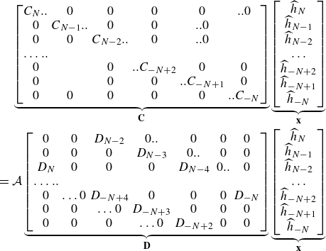 \begin{equation} \begin{aligned} \underbrace {\begin{bmatrix} C_N.. & 0 & 0 & 0 & 0 & ..0\\ 0 & C_{N-1}.. & 0 & 0 & ..0\\ 0 & 0 & C_{N-2}.. & 0 & ..0\\ \ldots ..\\ 0 & & 0 & ..C_{-N+2} & 0 & 0\\ 0 & & 0 & 0 & ..C_{-N+1} & 0\\ 0 & 0 & 0 & 0 & 0 & ..C_{-N}\\ \end{bmatrix}}_{\mathbf{C}} \underbrace {\begin{bmatrix} \widehat {h}_N \\ \widehat {h}_{N-1}\\ \widehat {h}_{N-2}\\ \ldots \\ \widehat {h}_{-N+2} \\ \widehat {h}_{-N+1} \\ \widehat {h}_{-N} \end{bmatrix}}_{\mathbf{x}} \\ =\mathcal{A} \underbrace {\begin{bmatrix} 0 & 0 & D_{N-2} & 0.. & 0 & 0 & 0\\ 0 & 0 & 0 & D_{N-3} & 0.. & 0 & 0\\ D_N & 0 & 0 & 0 & D_{N-4} & 0.. & 0\\ \ldots ..\\ 0 & \ldots 0 & D_{-N+4} & 0 & 0 & 0 & D_{-N} \\ 0 & 0 & \ldots 0 & D_{-N+3} & 0 & 0 & 0 \\ 0 & 0 & 0 & \ldots 0 & D_{-N+2} & 0 & 0\\ \end{bmatrix}}_{\mathbf{D}} \underbrace {\begin{bmatrix} \widehat {h}_N \\ \widehat {h}_{N-1}\\ \widehat {h}_{N-2}\\ \ldots \\ \widehat {h}_{-N+2} \\ \widehat {h}_{-N+1} \\ \widehat {h}_{-N} \end{bmatrix}}_{\mathbf{x}} \end{aligned} \end{equation}
where $C_n=(Re({i n \omega }/{2}) {\text{d}c_n }/{\text{d}z}\!-\!({1}/(1\!+{i n \omega } {De}/{2}))\; {d^3 c_n}/{\text{d}z^3}\! +\! ({3 k^2}/(1+{i n \omega } {De}/{2}))$ ${ \text{d}c_n }/{\text{d}z }+\mathcal{G} k^2+{k^4}/{{Ca}})\vert _{z=0}$
,
${ \text{d}c_n }/{\text{d}z }+\mathcal{G} k^2+{k^4}/{{Ca}})\vert _{z=0}$
, $c_n=\widehat {w}_n/\widehat {h}_n$
and
$c_n=\widehat {w}_n/\widehat {h}_n$
and $D_n={k^2}/{2}$
. Here
$D_n={k^2}/{2}$
. Here $n$
varies from
$n$
varies from $-N$
to
$-N$
to $N$
.
$N$
.


 Open access