





1. Introduction
Gravity current (GC) is a generic name for the buoyancy-driven flow of a fluid of one density, $\rho$
, into an ambient fluid of a different density,
$\rho$
, into an ambient fluid of a different density, $\rho _{a}$
, mostly in a horizontal or slightly inclined direction
$\rho _{a}$
, mostly in a horizontal or slightly inclined direction $x$
(to be distinguished from the mostly vertical buoyancy-driven flows called plumes); see Ungarish (Reference Ungarish2020, § 1) and the references therein. The interpretation of the driving buoyancy mechanism is as follows: the hydrostatic pressure fields
$x$
(to be distinguished from the mostly vertical buoyancy-driven flows called plumes); see Ungarish (Reference Ungarish2020, § 1) and the references therein. The interpretation of the driving buoyancy mechanism is as follows: the hydrostatic pressure fields $p_j \propto - \rho _j g z$
produce a horizontal pressure gradient
$p_j \propto - \rho _j g z$
produce a horizontal pressure gradient $\propto g' = |\rho /{\rho _{a}} - 1| g$
, where
$\propto g' = |\rho /{\rho _{a}} - 1| g$
, where $g$
is the gravitational acceleration,
$g$
is the gravitational acceleration, $z$
is the vertical upward coordinate,
$z$
is the vertical upward coordinate, $j$
denotes the ambient and current, and
$j$
denotes the ambient and current, and $g'$
is the reduced gravity. The buoyancy is balanced by inertial or viscous effects. Here, we focus attention on the so-called inertial GC, dominated by a buoyancy–inertia dynamic balance, relevant to flows at a large Reynolds number. Inertial GCs have numerous applications in geophysical and environmental systems (e.g. discharges of water of different temperature/salinity into lakes and oceans, propagation of smoke in tunnels, turbidity flows; see Simpson (Reference Snow and Sutherland1997), Huppert (Reference Huppert2000) for more details). The systems of interest belong to various prototypes, such as rectangular or cylindrical geometry, Boussinesq or non-Boussinesq, driven by compositional or suspended particles effects, in inertial or rotating systems (see Ungarish (Reference Ungarish2020, § 1.1)). Two important classification criteria are concerned with (i) the slope of the boundary over which propagation occurs, i.e. horizontal or inclined; and (ii) the type of the ambient fluid, i.e. homogeneous (constant
$g'$
is the reduced gravity. The buoyancy is balanced by inertial or viscous effects. Here, we focus attention on the so-called inertial GC, dominated by a buoyancy–inertia dynamic balance, relevant to flows at a large Reynolds number. Inertial GCs have numerous applications in geophysical and environmental systems (e.g. discharges of water of different temperature/salinity into lakes and oceans, propagation of smoke in tunnels, turbidity flows; see Simpson (Reference Snow and Sutherland1997), Huppert (Reference Huppert2000) for more details). The systems of interest belong to various prototypes, such as rectangular or cylindrical geometry, Boussinesq or non-Boussinesq, driven by compositional or suspended particles effects, in inertial or rotating systems (see Ungarish (Reference Ungarish2020, § 1.1)). Two important classification criteria are concerned with (i) the slope of the boundary over which propagation occurs, i.e. horizontal or inclined; and (ii) the type of the ambient fluid, i.e. homogeneous (constant $\rho _{a}$
) or stratified (
$\rho _{a}$
) or stratified ( $\rho _{a}$
decreases with the height
$\rho _{a}$
decreases with the height $z$
). Here, we focus attention on GCs over an inclined bottom that propagate into a linearly stratified fluid. A convenient and insightful prototype is the flow of a fixed volume released from behind a lock by the rapid opening of the front gate (dam-break), as sketched in figure 1.
$z$
). Here, we focus attention on GCs over an inclined bottom that propagate into a linearly stratified fluid. A convenient and insightful prototype is the flow of a fixed volume released from behind a lock by the rapid opening of the front gate (dam-break), as sketched in figure 1.
Sketch of the system with a ramp $x_{\textit{slope}} =x_0$
. The GC is initially (
$x_{\textit{slope}} =x_0$
. The GC is initially ( $t=0$
) in the lock (dashed line) of dimensions
$t=0$
) in the lock (dashed line) of dimensions $x_0, h_0$
. The detachment to intrusion is also sketched.
$x_0, h_0$
. The detachment to intrusion is also sketched.

The flow of lock-release GCs along a slope into a homogeneous ambient fluid has received a good deal of attention, and the literature reports insightful combination of experimental, numerical and modelling approaches (e.g. Birman et al. Reference Birman, Battandier, Meiburg and Linden2007; Maxworthy Reference Maxworthy2010; Dai Reference Dai2013; Zemach et al. Reference Zemach, Ungarish, Martin and Negretti2019; Han et al. Reference Han, He, Lin, Wang, Guo and Yuan2023; Gadal et al. Reference Gadal, Mercier, Rastello and Lacaze2023; Ungarish Reference Ungarish and Huppert2024b ). However, as pointed out by the recent review of He et al. (Reference He, Okon, Zhu, Pähtz and Meiburg2025), in many geophysical applications, the propagation occurs into a stratified ambient fluid and such systems have received little coverage. Notable attempts in this direction are the works of Snow & Sutherland (Reference Ungarish2014) and Ouillon et al. (Reference Ouillon, Meiburg and Sutherland2019) (the first experimental, the second numerical simulation, both concerned with particle-driven (turbidity) currents), and He et al. (Reference He, Zhao, Lin, Hu, lv, Ho and Lin2017) referred to subsequently as He2017 (a comprehensive experimental study concerned with compositional currents).
These recent laboratory, simulation and review papers of the flow of GCs along an inclined bottom in a lineally-stratified ambient have pointed out a serious gap of knowledge: there is no reliable theoretical model for such systems. In general, the major flow patterns of inertial GCs are fairly well predicted by shallow-water (SW) models (see Ungarish (Reference Ungarish2020, §§ 3, 7) and the references therein). However, the existing SW models for a stratified ambient are restricted to horizontal channels. The interpretations of the data of Snow & Sutherland (Reference Ungarish2014), Ouillon et al. (Reference Ouillon, Meiburg and Sutherland2019) and He2017 employ definitions and results of the horizontal GCs in stratified ambient, and show that some insights carry over. However, the ‘extrapolation’ of the available SW predictions from the horizontal to the inclined geometry is unreliable (and potentially misleading), because even when the slope angle $\gamma$
is small, the inclination contributes new terms to the momentum equation, front-jump condition and density dilution balance. The slope angle introduces some nonlinear couplings between effects (such as driving force and position) that have no counterpart in the previous SW studies. The system of interest is governed by many dimensionless parameters and, hence, a reliable analysis of the parametric behaviour for
$\gamma$
is small, the inclination contributes new terms to the momentum equation, front-jump condition and density dilution balance. The slope angle introduces some nonlinear couplings between effects (such as driving force and position) that have no counterpart in the previous SW studies. The system of interest is governed by many dimensionless parameters and, hence, a reliable analysis of the parametric behaviour for $\gamma \gt 0$
requires a predictive model that systematically incorporates the slope into the governing equation.
$\gamma \gt 0$
requires a predictive model that systematically incorporates the slope into the governing equation.
The basic SW-stratified model is an extension of the one-layer Boussinesq model for the homogeneous ambient (Ungarish & Huppert Reference van Reeuwijk, Holzner and Caulfield2002; Ungarish (Reference Ungarish2005); Ungarish Reference Ungarish2020, §§ 16, 18 and the references therein). The GC is represented by a thin layer of thickness $h(x,t)$
and the depth-averaged velocity is
$h(x,t)$
and the depth-averaged velocity is $u(x,t)$
. The ambient is assumed as a non-moving fluid of constant stratification measured by the dimensionless parameter
$u(x,t)$
. The ambient is assumed as a non-moving fluid of constant stratification measured by the dimensionless parameter $S \in [0,1]$
(defined by (2.3)). Here,
$S \in [0,1]$
(defined by (2.3)). Here, $S=0$
for the homogeneous limit and
$S=0$
for the homogeneous limit and $S=1$
is the maximum stratification (the density of the GC and
$S=1$
is the maximum stratification (the density of the GC and $\rho _{a}$
at the bottom of the lock coincide). The pressure in the fluids is hydrostatic and continuous at the interface. The SW equations of continuity and
$\rho _{a}$
at the bottom of the lock coincide). The pressure in the fluids is hydrostatic and continuous at the interface. The SW equations of continuity and $x$
-momentum form a hyperbolic set for
$x$
-momentum form a hyperbolic set for $h(x,t)$
and
$h(x,t)$
and $u(x,t)$
. At the nose
$u(x,t)$
. At the nose $x_N(t)$
, a Benjamin-type jump condition (Benjamin Reference Benjamin1968) is applied. With some straightforward modification, the theory developed for the flow over a bottom covers intrusions about the neutral buoyancy plane and GSs below a top (Agrawal et al. Reference Agrawal, Ungarish and Chalama2025). The typical solutions were concerned with lock-release problems. In dimensionless form, the classical horizontal flow (with no entrainment and no drag) depends on two parameters:
$x_N(t)$
, a Benjamin-type jump condition (Benjamin Reference Benjamin1968) is applied. With some straightforward modification, the theory developed for the flow over a bottom covers intrusions about the neutral buoyancy plane and GSs below a top (Agrawal et al. Reference Agrawal, Ungarish and Chalama2025). The typical solutions were concerned with lock-release problems. In dimensionless form, the classical horizontal flow (with no entrainment and no drag) depends on two parameters: $S$
and the height ratio
$S$
and the height ratio $H$
of ambient to lock. In general, the equations are amenable to a numerical (finite difference) solution, and analytical solutions are available for the initial slumping stage with constant
$H$
of ambient to lock. In general, the equations are amenable to a numerical (finite difference) solution, and analytical solutions are available for the initial slumping stage with constant $u_N$
and for the long-time similarity stage. Comparisons with data from experiments and Navier–Stokes simulations, for both GCs and intrusions, show fair agreement over a wide range of parameters. The main deficiencies of the theory are that the return flow and the internal stratification waves in the ambient are neglected. However, in many cases of interest, these effects are small during a significant period and length of propagation. While the SW formulation for the homogeneous ambient (
$u_N$
and for the long-time similarity stage. Comparisons with data from experiments and Navier–Stokes simulations, for both GCs and intrusions, show fair agreement over a wide range of parameters. The main deficiencies of the theory are that the return flow and the internal stratification waves in the ambient are neglected. However, in many cases of interest, these effects are small during a significant period and length of propagation. While the SW formulation for the homogeneous ambient ( $S=0$
) has been successfully extended for GCs over an inclined bottom (Zemach et al. Reference Zemach, Ungarish, Martin and Negretti2019; Ungarish Reference Ungarish2020), no such extension has been presented and tested for the
$S=0$
) has been successfully extended for GCs over an inclined bottom (Zemach et al. Reference Zemach, Ungarish, Martin and Negretti2019; Ungarish Reference Ungarish2020), no such extension has been presented and tested for the $S\gt 0$
systems. This gap of knowledge has motivated the present study. We note that He2017 attempted a theoretical interpretation of the motion of the front by means of the ‘thermal theory’ (Beghin, Hopfinger & Britter Reference Beghin, Hopfinger and Britter1981). This approach is based on global balances that are reduced to ordinary differential equations. After some calibration, the thermal model reproduces well the propagation during the deceleration stage; however, this formulation does not satisfy initial conditions and cannot predict accurately the initial stage of propagation (sometimes referred to as slumping stage). For more details, see Ungarish (Reference Ungarish2020, § 11.2.3) and Ungarish (Reference Ungarish2024a
). Here, we present a different model, based on local balances (partial differential equations), which admits realistic initial and boundary conditions, and is valid for the entire propagation.
$S\gt 0$
systems. This gap of knowledge has motivated the present study. We note that He2017 attempted a theoretical interpretation of the motion of the front by means of the ‘thermal theory’ (Beghin, Hopfinger & Britter Reference Beghin, Hopfinger and Britter1981). This approach is based on global balances that are reduced to ordinary differential equations. After some calibration, the thermal model reproduces well the propagation during the deceleration stage; however, this formulation does not satisfy initial conditions and cannot predict accurately the initial stage of propagation (sometimes referred to as slumping stage). For more details, see Ungarish (Reference Ungarish2020, § 11.2.3) and Ungarish (Reference Ungarish2024a
). Here, we present a different model, based on local balances (partial differential equations), which admits realistic initial and boundary conditions, and is valid for the entire propagation.
The extension of the SW model for the propagation in a stratification over an inclined bottom poses several challenges which were not encountered in the counterpart systems (inclined unstratified and horizontal stratified). Let us briefly recall some major patterns of motion of the lock-release inertial Boussinesq GC in a homogeneous ambient, in a tank whose upper boundary (top) is horizontal and open to the atmosphere. When $\gamma = 0$
, after a short acceleration, the speed of the nose,
$\gamma = 0$
, after a short acceleration, the speed of the nose, $u_N$
, is constant in the so-called slumping stage during which the nose advances a few lock-lengths; then, after another short adjustment,
$u_N$
, is constant in the so-called slumping stage during which the nose advances a few lock-lengths; then, after another short adjustment, $u_N \sim t^{-1/3}$
for a long propagation called the similarity stage. While the GC becomes slow and thin, the influence of the viscous forces increases and eventually a transition from the inertial to viscous regime occurs. Experiments and theory indicate that the interfacial mixing/entrainment and drag, while present, remain small during fairly long propagations (Johnson & Hogg Reference Johnson and Hogg2013). When
$u_N \sim t^{-1/3}$
for a long propagation called the similarity stage. While the GC becomes slow and thin, the influence of the viscous forces increases and eventually a transition from the inertial to viscous regime occurs. Experiments and theory indicate that the interfacial mixing/entrainment and drag, while present, remain small during fairly long propagations (Johnson & Hogg Reference Johnson and Hogg2013). When $\gamma \gt 0$
, the pattern is more complicated: (i) the slope contributes additional acceleration, which destabilises the interface, and hence entrainment and drag terms become relevant from the beginning (Maxworthy & Nokes Reference Maxworthy and Nokes2007; Baines Reference Baines2008); (ii) due to the slope, the height of the ambient encountered by the nose increases with time (distance). Due to the effects (i) and (ii) in the slumping stage,
$\gamma \gt 0$
, the pattern is more complicated: (i) the slope contributes additional acceleration, which destabilises the interface, and hence entrainment and drag terms become relevant from the beginning (Maxworthy & Nokes Reference Maxworthy and Nokes2007; Baines Reference Baines2008); (ii) due to the slope, the height of the ambient encountered by the nose increases with time (distance). Due to the effects (i) and (ii) in the slumping stage, $u_N$
is rather increasing than constant (but only slightly, because the slope perturbations are usually small). Eventually, the drag and entrainment become dominant and a similarity stage with
$u_N$
is rather increasing than constant (but only slightly, because the slope perturbations are usually small). Eventually, the drag and entrainment become dominant and a similarity stage with $u_N \sim t^{-1/3}$
appears again (but with a different mechanism from the
$u_N \sim t^{-1/3}$
appears again (but with a different mechanism from the $\gamma = 0$
case). See Maxworthy (Reference Maxworthy2010), Dai (Reference Dai2013), Han et al. (Reference Han, He, Lin, Wang, Guo and Yuan2023), Gadal et al. (Reference Gadal, Mercier, Rastello and Lacaze2023), Ungarish (Reference Ungarish2024a
,
Reference Ungarish and Huppertb
).
$\gamma = 0$
case). See Maxworthy (Reference Maxworthy2010), Dai (Reference Dai2013), Han et al. (Reference Han, He, Lin, Wang, Guo and Yuan2023), Gadal et al. (Reference Gadal, Mercier, Rastello and Lacaze2023), Ungarish (Reference Ungarish2024a
,
Reference Ungarish and Huppertb
).
The stratification of the ambient in the donwslope system introduces some evidently novel features. First, as expected and observed in experiments, the GC with $S\gt 0, \gamma \gt 0$
detaches from the bottom at some
$S\gt 0, \gamma \gt 0$
detaches from the bottom at some $z_d$
and then propagates horizontally as an intrusion. Second, the inclined bottom renders the top-to-bottom density change in the ambient dependent on
$z_d$
and then propagates horizontally as an intrusion. Second, the inclined bottom renders the top-to-bottom density change in the ambient dependent on $x$
, and this opens various options for the stratification parameter. Third, the jump condition at the nose must take into account the fact that the driving effective reduced gravity decreases while the nose moves into larger
$x$
, and this opens various options for the stratification parameter. Third, the jump condition at the nose must take into account the fact that the driving effective reduced gravity decreases while the nose moves into larger $\rho _{a}$
. Fourth, the closures for drag and entrainment, which are considered essential components in the donwslope motion, are uncertain for the stratified systems. In the unstratified case, the entrained fluid is of constant
$\rho _{a}$
. Fourth, the closures for drag and entrainment, which are considered essential components in the donwslope motion, are uncertain for the stratified systems. In the unstratified case, the entrained fluid is of constant $\rho _{a}$
, while in the stratified case, the density of the entrained fluid changes along the slope.
$\rho _{a}$
, while in the stratified case, the density of the entrained fluid changes along the slope.
Our model suggests practical remedies to these problems. The resulting system of equations is self-contained and amenable to numerical solution by standard methods. The clear-cut predictions are compared with experimental data. Overall, there is fair agreement, which gives confidence that the present model captures well the mechanisms of the flowfield.
The structure of the paper is as follow. The SW governing equations and boundary conditions are formulated in § 2. Predictions and comparisons with data are presented and discussed in § 3. Section 4 gives some concluding remarks and suggestions for further work. Some guiding lines for the incorporation of settling particles in the model are presented in Appendix A. The characteristics of the SW system are given in Appendix B.
2. Formulation
2.1. Governing equations
We use dimensional variables unless stated otherwise. The variables of the ambient fluid are denoted by the subscript $a$
, while those of the current are without subscript (or with subscript
$a$
, while those of the current are without subscript (or with subscript $c$
when emphasis is needed). We use the Cartesian
$c$
when emphasis is needed). We use the Cartesian $xz$
two-dimensional (2-D) system with
$xz$
two-dimensional (2-D) system with $x$
horizontal and
$x$
horizontal and $z$
vertically upward, and corresponding
$z$
vertically upward, and corresponding $u,w$
velocity components. Gravity
$u,w$
velocity components. Gravity $g$
acts in the -
$g$
acts in the - $z$
direction. The geometry is as follows (figure 1). The top and bottom of the channel are at
$z$
direction. The geometry is as follows (figure 1). The top and bottom of the channel are at $z=z_T =H_0$
and
$z=z_T =H_0$
and $z_B(x)$
, with
$z_B(x)$
, with $z_B(0) = 0$
. The height and slope of the channel are
$z_B(0) = 0$
. The height and slope of the channel are
 \begin{align} H = H(x) = z_T - z_B(x), \quad \gamma = \gamma (x) = - \frac {\text{d} z_B}{\text{d}x}. \end{align}
For simplicity, and in accord with the laboratory systems relevant to this paper, we assume that $\gamma = 0$
for
$\gamma = 0$
for $x\lt x_{\textit{slope}}$
(a ramp) and a constant for larger
$x\lt x_{\textit{slope}}$
(a ramp) and a constant for larger $x$
. The lock is defined by the backwall
$x$
. The lock is defined by the backwall $x=0$
, dam (gate) at
$x=0$
, dam (gate) at $x=x_0$
and is of height
$x=x_0$
and is of height $h_0$
above the bottom. We shall assume a constant
$h_0$
above the bottom. We shall assume a constant $h_0$
.
$h_0$
.
The line (plane) $z=0$
, which is the bottom of the ramp, is a convenient reference. Let
$z=0$
, which is the bottom of the ramp, is a convenient reference. Let $H_0 = H(x=0)$
be the height of the top of the tank with respect to that reference.
$H_0 = H(x=0)$
be the height of the top of the tank with respect to that reference.
The density of the ambient, ${\rho _{a}}(z)$
, increases linearly from
${\rho _{a}}(z)$
, increases linearly from $\rho _{o}$
at the top
$\rho _{o}$
at the top $z = H_0$
to larger values at the bottom, as follows:
$z = H_0$
to larger values at the bottom, as follows:
 \begin{align} {\rho _{a}}(z) = {\rho _{o}} + {\widetilde {\Delta \rho }} \ \left(1- \frac {z}{H_0}\right), \quad (z_B(x) \leqslant z \leqslant z_T = H_0). \end{align}
The parameter $\widetilde {\Delta \rho }$
is the density increase from the top to the level of the ramp and
$\widetilde {\Delta \rho }$
is the density increase from the top to the level of the ramp and ${\widetilde {\Delta \rho }}/H_0 = -\text{d} {\rho _{a}}/ \text{d}z$
is the stratification gradient. In our analysis, the density field in the ambient is fixed by (2.2) (independent of time), because we use a one-layer SW model which assumes that the motion in the ambient fluid is negligible.
${\widetilde {\Delta \rho }}/H_0 = -\text{d} {\rho _{a}}/ \text{d}z$
is the stratification gradient. In our analysis, the density field in the ambient is fixed by (2.2) (independent of time), because we use a one-layer SW model which assumes that the motion in the ambient fluid is negligible.
The initial density of the current (at time $t=0$
, in the lock) is
$t=0$
, in the lock) is ${\rho _{c0}} \ (\geqslant {\rho _{a}}(0))$
. The stratification parameter of the system is defined by
${\rho _{c0}} \ (\geqslant {\rho _{a}}(0))$
. The stratification parameter of the system is defined by
 \begin{align} S = \frac {{\rho _{a}}(z = 0) - {\rho _{o}}}{{\rho _{c0}} - {\rho _{o}}} = \frac {{\widetilde {\Delta \rho }}}{{\rho _{c0}} - {\rho _{o}}}. \end{align}
This definition is convenient because: (i) the range of $S$
is the standard
$S$
is the standard $[0,1]$
, where
$[0,1]$
, where $S=0$
means no stratification (
$S=0$
means no stratification ( ${\widetilde {\Delta \rho }} = 0)$
and for
${\widetilde {\Delta \rho }} = 0)$
and for $S=1$
(maximum stratification), the density in the lock equals
$S=1$
(maximum stratification), the density in the lock equals ${\rho _{a}}(z=0)$
, which implies that the lock-release will form an intrusion from the beginning; (ii) consistency with the existing formulation for the non-inclined system is preserved.
${\rho _{a}}(z=0)$
, which implies that the lock-release will form an intrusion from the beginning; (ii) consistency with the existing formulation for the non-inclined system is preserved.
We use $\rho$
(with no subscripts) to denote the density of the current. The initial value
$\rho$
(with no subscripts) to denote the density of the current. The initial value $\rho _{c0}$
of the lock is diluted during the propagation by entertainment. This change of
$\rho _{c0}$
of the lock is diluted during the propagation by entertainment. This change of $\rho$
is modelled by
$\rho$
is modelled by
 \begin{align} \rho (x,t) = {\rho _{o}} +({\rho _{c0}} - {\rho _{o}}) \phi (x,t) = {\rho _{o}} + \frac {{\widetilde {\Delta \rho }}}{S} \phi (x,t), \end{align}
where $\phi$
expresses the concentration of the dense component in the GC. Initially,
$\phi$
expresses the concentration of the dense component in the GC. Initially, $\phi (t=0) = 1$
and, subsequently,
$\phi (t=0) = 1$
and, subsequently, $\phi (x,t)$
is expected to decay with
$\phi (x,t)$
is expected to decay with $x$
and
$x$
and $t$
.
$t$
.
We introduce the reference reduced gravity
 \begin{align} g_0' = \frac {{\rho _{c0}} - {\rho _{o}}}{{\rho _{o}}} g = \frac {{\widetilde {\Delta \rho }}}{S} g, \end{align}
and the buoyancy frequency
 \begin{align} {\mathcal{N}} = \left ( - \frac {g}{{\rho _{o}}} \frac {{\rm d} {\rho _{a}}}{\text{d}z} \right ) ^{1/2} = \left ( \frac {S g'_0}{H_0} \right ) ^{1/2}. \end{align}
The effective reduced gravity for a particle of dense fluid is $\propto \rho -{\rho _{a}}(z \approx z_B)$
, and is expected to vary significantly with
$\propto \rho -{\rho _{a}}(z \approx z_B)$
, and is expected to vary significantly with $x$
and
$x$
and $t$
. However,
$t$
. However, $\mathcal{N}$
of the stratified fluid is constant.
$\mathcal{N}$
of the stratified fluid is constant.
The balance SW equations consider a quite general system; see Ungarish (Reference Ungarish2020, §§ 11, 16). Since the GC is assumed as a thin layer of height $h(x,t)$
, attention is focused on the longitudinal behaviour for the depth-averaged
$h(x,t)$
, attention is focused on the longitudinal behaviour for the depth-averaged $u(x,t)$
and
$u(x,t)$
and $\phi (x,t)$
, where
$\phi (x,t)$
, where $t$
is the time from the release (dam-break) occurrence. Our objective is to predict the variables
$t$
is the time from the release (dam-break) occurrence. Our objective is to predict the variables $h, u, \phi$
for the CG. The position
$h, u, \phi$
for the CG. The position $x_N(t)$
is the by-product time-integral of
$x_N(t)$
is the by-product time-integral of $u_N(t)$
(the subscript
$u_N(t)$
(the subscript $N$
denotes the nose of the GC).
$N$
denotes the nose of the GC).
The thin-layer hypothesis implies $|w/u| \ll 1$
, where
$|w/u| \ll 1$
, where $w$
is the vertical velocity. We note that for consistency with the
$w$
is the vertical velocity. We note that for consistency with the $|w/u| \ll 1$
assumption, we must also assume that the entrainment coefficient
$|w/u| \ll 1$
assumption, we must also assume that the entrainment coefficient $E$
(see later) is small and the slope angle
$E$
(see later) is small and the slope angle $\gamma$
is not large (for definiteness, let
$\gamma$
is not large (for definiteness, let $\gamma \lt 0.2 \approx 12^\circ$
). We therefore use the horizontal–vertical coordinates system; the transformation to the along-slope system involves a small
$\gamma \lt 0.2 \approx 12^\circ$
). We therefore use the horizontal–vertical coordinates system; the transformation to the along-slope system involves a small $O(1 - \cos \gamma )$
difference, which we ignore. The
$O(1 - \cos \gamma )$
difference, which we ignore. The $x{-}z$
system is convenient for the incorporation of the stratification and hydrostatic-pressure terms. Let
$x{-}z$
system is convenient for the incorporation of the stratification and hydrostatic-pressure terms. Let $q = uh$
. The volume continuity equation of the current is
$q = uh$
. The volume continuity equation of the current is
 \begin{align} \frac {{\partial } h}{{\partial } t} +\frac {{\partial } q}{{\partial } x} = E |u|, \end{align}
where $E$
is a dimensionless entrainment coefficient (to be specified later). The modelled entrainment at volume rate
$E$
is a dimensionless entrainment coefficient (to be specified later). The modelled entrainment at volume rate $E|u|$
occurs at the interface
$E|u|$
occurs at the interface $z = z_B + h$
, and hence, the entrained density varies with
$z = z_B + h$
, and hence, the entrained density varies with $x$
and
$x$
and $t$
. Keeping this in mind, the mass (dense component) balance is expressed as
$t$
. Keeping this in mind, the mass (dense component) balance is expressed as
 \begin{align} \frac {{\partial } \rho h }{{\partial } t} +\frac {{\partial } \rho q }{{\partial } x} = E |u| {\rho _{a}}(z_B+h). \end{align}
A more convenient form is obtained by substituting (2.2)–(2.4), and using (2.7) and (2.3), as follows:
 \begin{align} \frac {{\partial } \phi h }{{\partial } t} +\frac {{\partial } \phi q }{{\partial } x} = S E |u| \left ( 1- \frac {z_B+h}{H_0} \right )\!. \end{align}
The momentum equations need some manipulations. Again, we assume that shear terms and motion in the ambient are negligible and the GC is a thin layer $(h /x_N \ll 1)$
. The driving force for
$(h /x_N \ll 1)$
. The driving force for $u$
is provided by the
$u$
is provided by the $x$
-component of the pressure gradient and, hence, we first focus attention on this variable. Following our assumptions, (i) the
$x$
-component of the pressure gradient and, hence, we first focus attention on this variable. Following our assumptions, (i) the $Dw/Dt$
acceleration is very small and, hence, the
$Dw/Dt$
acceleration is very small and, hence, the $z$
-momentum equation is reduced to the hydrostatic pressure balance,
$z$
-momentum equation is reduced to the hydrostatic pressure balance, ${\partial } p_j /{\partial } z = - \rho_j g, \ (j = a,c)$
, where
${\partial } p_j /{\partial } z = - \rho_j g, \ (j = a,c)$
, where $p$
is the pressure; (ii) the pressure is continuous,
$p$
is the pressure; (ii) the pressure is continuous, $p_c(x,t,z) = p_a(z)$
, at the interface
$p_c(x,t,z) = p_a(z)$
, at the interface $z = z_B(x) + h(x,t)$
. Consequently,
$z = z_B(x) + h(x,t)$
. Consequently,
 \begin{align} p_a(z) &= -g \left [ ({\rho _{o}} + {\widetilde {\Delta \rho }}) z - {\frac {1}{2}} {\widetilde {\Delta \rho }} \frac {z^2}{H_0} \right ]\!, \\[-12pt]\nonumber \end{align}
 \begin{align} p_c(x,z,t) =& p_a(z_B + h) + \rho (x,t) g \boldsymbol{\cdot }(z_B + h -z). \end{align}
We used (2.2) and note that the density $\rho$
of the dense fluid is given by (2.4). (The constant of integration in (2.10) was set zero.) We calculate
$\rho$
of the dense fluid is given by (2.4). (The constant of integration in (2.10) was set zero.) We calculate ${\partial } p_c/ {\partial } x$
and then average (denoted here by an overline) over the thickness of the layer. We obtain
${\partial } p_c/ {\partial } x$
and then average (denoted here by an overline) over the thickness of the layer. We obtain
 \begin{align} -\overline { \frac {{\partial } p_c}{{\partial } x} }(x,t) = {\rho _{o}} g_0' \left \{ \left [ \phi - S + S \frac {z_B + h} {H_0} \right ] \left ( - \frac {{\partial } h}{{\partial } x} + \gamma \right ) - \frac {h}{2} \frac {{\partial } \phi }{{\partial } x} \right \}\!. \end{align}
Equation (2.12) determines then the driving effect (buoyancy) of the dense fluid. We note that the driving term is affected by a combination of variables. We keep in mind that $z_B$
is negative. The inclination
$z_B$
is negative. The inclination $(-{\partial } h/{\partial } x + \gamma )$
pushes the current forward, and the term in the right brackets expresses the strength of the density contrast (the cause of the buoyancy) between the dense fluid and the ambient. This term decreases as (i)
$(-{\partial } h/{\partial } x + \gamma )$
pushes the current forward, and the term in the right brackets expresses the strength of the density contrast (the cause of the buoyancy) between the dense fluid and the ambient. This term decreases as (i) $S$
increases (stronger stratification), (ii)
$S$
increases (stronger stratification), (ii) $\phi$
decreases (dilution) and (iii)
$\phi$
decreases (dilution) and (iii) $z_B$
decreases (the density of the ambient increases along the bottom).
$z_B$
decreases (the density of the ambient increases along the bottom).
That driving term (2.12) is counteracted by (i) the depth-averaged acceleration (inertia) and (ii) a drag term. Using the Boussinesq simplification ( $\rho {\rm D}u/{\rm D}t \approx \rho _o {\rm D}u/{\rm D}t$
), we obtain the SW
$\rho {\rm D}u/{\rm D}t \approx \rho _o {\rm D}u/{\rm D}t$
), we obtain the SW $x$
-momentum equation
$x$
-momentum equation
 \begin{align} \frac {{\partial } q }{{\partial } t} + \frac {{\partial } (q^2/ h) } {{\partial } x} = g'_0 h \left \{ \left [ \phi - S + S \frac {z_B + h} {H_0} \right ] \left ( - \frac {{\partial } h}{{\partial } x} + \gamma \right ) - \frac {h}{2} \frac {{\partial } \phi }{{\partial } x} \right \} - c_D u |u|, \end{align}
where $c_D$
is a drag coefficient.
$c_D$
is a drag coefficient.
For closing the system, we need a front-jump condition and correlations for $c_D$
and
$c_D$
and $E$
.
$E$
.
The need for the front condition in the hyperbolic SW model (see Appendix B) has been discussed in the literature (e.g. Klemp, Rotunno & Skamarock Reference Klemp, Rotunno and Skamarock1994; Ungarish Reference Ungarish2020, § 3.1.2)). Briefly, after the dam-break lock-release, the back-moving characteristics generate a smooth expansion wave into the reservoir, while the forward-moving characteristics intersect and generate a jump which propagates into the ambient fluid. A rigorous formula for the jump condition in the presence of stratification is not available. Inspired by the model for the horizontal bottom, we use the conjecture (see Ungarish Reference Ungarish2020, § 16.2.1)
 \begin{align} u_N = \frac {\text{d} x_N}{\text{d} t} = \textit{Fr}(a) \left [ \frac { p_c(x,z_B,t) - p_a(z_B)}{{\rho _{o}}} \right ]^{1/2}, \end{align}
where $a = h_N/H(x_N)$
at the nose and
$a = h_N/H(x_N)$
at the nose and $\textit{Fr}(a)$
is a nose-Froude number formula. In view of (2.10) and (2.11), we obtain
$\textit{Fr}(a)$
is a nose-Froude number formula. In view of (2.10) and (2.11), we obtain
 \begin{align} u_N = \textit{Fr}(a) \left [ \phi - S \left ( 1 - {\frac {1}{2}} \frac {h}{H_0} \right ) + S \frac {z_B}{H_0} \right ] ^{1/2} (g'_0 h)^{1/2}, \end{align}
where $h, \phi$
and
$h, \phi$
and $z_B$
are the values at
$z_B$
are the values at $x_N$
. The Huppert & Simpson (Reference Huppert and Simpson1980) study provides the convenient semi-empirical formula
$x_N$
. The Huppert & Simpson (Reference Huppert and Simpson1980) study provides the convenient semi-empirical formula
 \begin{align} \textit{Fr}(a) = 0.5 a^{-1/3} \quad (0.075\lt a \leqslant 1), \quad \textit{Fr}(a) = 1.19 \quad (a \leqslant 0. 075). \end{align}
For $z_B =0$
, (2.15) recovers the
$z_B =0$
, (2.15) recovers the $u_N$
prediction for a horizontal propagation in a stratified ambient, which has been successfully tested (e.g. Ungarish & Huppert Reference van Reeuwijk, Holzner and Caulfield2002). The inclined bottom introduces two additional physical effects. While the GC propagates along the slope,
$u_N$
prediction for a horizontal propagation in a stratified ambient, which has been successfully tested (e.g. Ungarish & Huppert Reference van Reeuwijk, Holzner and Caulfield2002). The inclined bottom introduces two additional physical effects. While the GC propagates along the slope, $z_B$
decreases and the height
$z_B$
decreases and the height $H(x)$
of the ambient increases. The negative
$H(x)$
of the ambient increases. The negative $z_B$
reduces the driving-force term in the right brackets. However, the larger
$z_B$
reduces the driving-force term in the right brackets. However, the larger $H$
is expected to reduce
$H$
is expected to reduce $a$
and thus increase
$a$
and thus increase $\textit{Fr}$
. Since
$\textit{Fr}$
. Since $u_N$
also depends on the changing
$u_N$
also depends on the changing $h_N$
and
$h_N$
and $\phi _N$
, it is evident that a non-monotonic variation of
$\phi _N$
, it is evident that a non-monotonic variation of $u_N$
, influenced by various parameters (
$u_N$
, influenced by various parameters ( $S, \gamma , E, c_D$
and more) may occur.
$S, \gamma , E, c_D$
and more) may occur.
We switch to dimensionless variables, defined as follows: $x$
is scaled with
$x$
is scaled with $x_0$
, heights with
$x_0$
, heights with $h_0$
, velocity with
$h_0$
, velocity with $U = (g_0' h_0)^{1/2}$
, time with
$U = (g_0' h_0)^{1/2}$
, time with $T = x_0/U$
and volume with
$T = x_0/U$
and volume with $x_0 h_0$
. Since the vertical and horizontal lengths are scaled differently, the aspect ratio of the lock,
$x_0 h_0$
. Since the vertical and horizontal lengths are scaled differently, the aspect ratio of the lock, $\lambda = x_0/h_0$
, enters into the governing equation (actually, into the source terms). The initial Reynolds number is
$\lambda = x_0/h_0$
, enters into the governing equation (actually, into the source terms). The initial Reynolds number is $Uh_0\nu$
, assumed large, where
$Uh_0\nu$
, assumed large, where $\nu$
is the kinematic viscosity. For simplicity, in the momentum equation, we represent the slope by
$\nu$
is the kinematic viscosity. For simplicity, in the momentum equation, we represent the slope by $\gamma$
.
$\gamma$
.
It is also convenient to introduce the variable $\varphi = \phi h$
, which expresses the buoyancy of the GC at the position
$\varphi = \phi h$
, which expresses the buoyancy of the GC at the position $x$
at time
$x$
at time $t$
. Recall,
$t$
. Recall, $u = q/h$
.
$u = q/h$
.
In dimensionless conservation form, the governing equations for the variable $h, \varphi , q$
read
$h, \varphi , q$
read
 \begin{align} &\hspace{3.5pc} \frac {{\partial } h}{{\partial } t} +\frac {{\partial } q}{{\partial } x} = \lambda E |u|, \\[-12pt]\nonumber \end{align}
 \begin{align} &\hspace{2pc} \frac {{\partial } \varphi }{{\partial } t} + \frac {{\partial } \varphi u }{{\partial } x} = S \lambda E |u| \left ( 1- \frac {z_B+h}{H_0} \right )\!, \\[-12pt]\nonumber \end{align}
 \begin{align} &\frac {{\partial } q }{{\partial } t} + \frac {{\partial } \ }{{\partial } x} \left [ \frac {q^2}{h} + {\frac {1}{2}} \varphi h - {\frac {1}{2}} \textit{Sh}^2 \left ( 1 - \frac {z_B}{H_0} - \frac {2}{3} \frac {h}{H_0} \right ) \right ] \\[-12pt]\nonumber \\ &\hspace{2pc}=\lambda \gamma \left [ \varphi - \textit{Sh} \left ( 1 - \frac {z_B}{H_0} - {\frac {1}{2}} \frac {h}{H_0}\right ) \right ] - \lambda c_D u|u|. \end{align}
The relevant characteristics are considered in Appendix B. The system is expected to be of hyperbolic type in the domain of interest (from release to detachment).
The dimensionless form of the nose condition is
 \begin{align} u_N = \frac {\text{d} x_N}{\text{d}t} = \textit{Fr}(a) \left [ \varphi - \textit{Sh} \left ( 1 - {\frac {1}{2}} \frac {h}{H_0} \right ) + S h \frac {z_B}{H_0} \right ] ^{1/2}, \end{align}
where $h, \varphi , z_B$
and
$h, \varphi , z_B$
and $a$
are the values at
$a$
are the values at $x_N$
.
$x_N$
.
The negative term $z_B/H_0$
(which decreases with
$z_B/H_0$
(which decreases with $x-x_{\textit{slope}}$
) represents the change of the ambient-fluid density along the slope. We note that the contribution of this term is always multiplied by
$x-x_{\textit{slope}}$
) represents the change of the ambient-fluid density along the slope. We note that the contribution of this term is always multiplied by $S$
, which could be expected. This term affects the density dilution, momentum equation (on both right and left sides) and the nose condition. This coupling of effects emphasises the need of a predictive model for the analysis of the motion in the inclined-stratified circumstances.
$S$
, which could be expected. This term affects the density dilution, momentum equation (on both right and left sides) and the nose condition. This coupling of effects emphasises the need of a predictive model for the analysis of the motion in the inclined-stratified circumstances.
The terms associated with $E, c_D$
and
$E, c_D$
and $\gamma$
are referred to as ‘source terms’ for obvious reasons; we reiterate that, physically, a negative source is a sink. In practice, we have control (or reliable knowledge) on the values of
$\gamma$
are referred to as ‘source terms’ for obvious reasons; we reiterate that, physically, a negative source is a sink. In practice, we have control (or reliable knowledge) on the values of $\gamma$
and
$\gamma$
and $S$
, while
$S$
, while $E$
and
$E$
and $c_D$
are provided by some indirect (and less reliable) estimates on which we have no control. In any case, there is good evidence that
$c_D$
are provided by some indirect (and less reliable) estimates on which we have no control. In any case, there is good evidence that $E$
and
$E$
and $c_D$
are small for typical Boussinesq GCs (Johnson & Hogg Reference Johnson and Hogg2013; Negretti, Flor & Hopfinger Reference Negretti, Flor and Hopfinger2017; Martin et al. Reference Martin, Negretti, Ungarish and Zemach2020). Consequently, it is justified to assume that the source terms in our analysis are small. However, the contribution of the source terms accumulates and may become significant for large
$c_D$
are small for typical Boussinesq GCs (Johnson & Hogg Reference Johnson and Hogg2013; Negretti, Flor & Hopfinger Reference Negretti, Flor and Hopfinger2017; Martin et al. Reference Martin, Negretti, Ungarish and Zemach2020). Consequently, it is justified to assume that the source terms in our analysis are small. However, the contribution of the source terms accumulates and may become significant for large $t$
.
$t$
.
The coefficients $c_D$
and
$c_D$
and $E$
are attributed to interfacial instabilities associated with the local bulk Richardson number,
$E$
are attributed to interfacial instabilities associated with the local bulk Richardson number, $Ri(x,t)$
. The relevant density difference is
$Ri(x,t)$
. The relevant density difference is $\delta \rho = \rho (x,t) - {\rho _{a}}(z_B+ h)$
. Assuming that the relevant height scale of instability perturbations is
$\delta \rho = \rho (x,t) - {\rho _{a}}(z_B+ h)$
. Assuming that the relevant height scale of instability perturbations is $h(x,t)$
, the formal ratio
$h(x,t)$
, the formal ratio $\delta \rho gh/\rho_o u^2$
(dimensional) is reduced to the expression (using dimensionless variables)
$\delta \rho gh/\rho_o u^2$
(dimensional) is reduced to the expression (using dimensionless variables)
 \begin{align} Ri = Ri(x,t) = \frac {\varphi - \textit{Sh} [ 1 - (z_B + h)/H_0]}{{u}^2}. \end{align}
For $c_D$
, we use a constant value, 0.10, suggested by the experimental data of Negretti et al. (Reference Negretti, Flor and Hopfinger2017), and numerical tests with some different values confirmed its robustness. For entrainment, we employ the correlation
$c_D$
, we use a constant value, 0.10, suggested by the experimental data of Negretti et al. (Reference Negretti, Flor and Hopfinger2017), and numerical tests with some different values confirmed its robustness. For entrainment, we employ the correlation
 \begin{align} E = \frac {E_0}{1 + k Ri}, \end{align}
with $E_0 = 0.075, k= 27$
, derived by Johnson & Hogg (Reference Johnson and Hogg2013) from empirical data over a fairly large range of parameters. We emphasise that the correlation for
$E_0 = 0.075, k= 27$
, derived by Johnson & Hogg (Reference Johnson and Hogg2013) from empirical data over a fairly large range of parameters. We emphasise that the correlation for $c_D$
and (2.22) were obtained for homogeneous fluids. Here, we extend the use of these correlations to the stratified system as a tentative plausible closure for the mathematical model. This closure assumption awaits confirmation and improvement. These are empirical correlations with adjustable constants. In this sense, the SW formulation is not self-contained. However,
$c_D$
and (2.22) were obtained for homogeneous fluids. Here, we extend the use of these correlations to the stratified system as a tentative plausible closure for the mathematical model. This closure assumption awaits confirmation and improvement. These are empirical correlations with adjustable constants. In this sense, the SW formulation is not self-contained. However, $E$
and
$E$
and $c_D$
are expected to be some generic functions, of broad validity, that can be determined by experiments and direct numerical sumulation computations in the future, rather than some undetermined parameters that should be calibrated again and again for any particular GC. We shall keep the same
$c_D$
are expected to be some generic functions, of broad validity, that can be determined by experiments and direct numerical sumulation computations in the future, rather than some undetermined parameters that should be calibrated again and again for any particular GC. We shall keep the same $E$
and
$E$
and $c_D$
for all the comparisons made in this work. We emphasise that the SW model is not restricted to these particular closures for
$c_D$
for all the comparisons made in this work. We emphasise that the SW model is not restricted to these particular closures for $E$
and
$E$
and $c_D$
, and other correlations can be used when more information will be available.
$c_D$
, and other correlations can be used when more information will be available.
An inspection of the equations reveals that the analysis of the propagation of the GC is, in general, a complex task. Even under the one-layer Boussinesq simplification, the flow is governed by a large number of dimensionless parameters: the stratification $S$
, slope
$S$
, slope $\gamma$
, the changing height
$\gamma$
, the changing height $H(x)$
, the entrainment correlation
$H(x)$
, the entrainment correlation $E(Ri)$
, the drag coefficient
$E(Ri)$
, the drag coefficient $c_D$
and the lock aspect ratio
$c_D$
and the lock aspect ratio $\lambda =(x_0/h_0)$
.
$\lambda =(x_0/h_0)$
.
2.2. Detachment and intrusion
The governing equations (2.9), (2.13) and (2.15) (and the dimensionless counterparts) are valid for a restricted domain of $x_N$
and time. Some time after release, the nose
$x_N$
and time. Some time after release, the nose $x_N(t)$
reaches the level of matching densities between the current and the ambient,
$x_N(t)$
reaches the level of matching densities between the current and the ambient, $\rho = {\rho _{a}}(z)$
. This defines, using (2.2) and (2.4), the detachment (subscript
$\rho = {\rho _{a}}(z)$
. This defines, using (2.2) and (2.4), the detachment (subscript $d$
) position
$d$
) position
 \begin{align} -\frac {z_{d}}{H_0} = \frac {\phi }{S} - 1, \quad x_d = x_{\textit{slope}} - \frac {z_d}{\lambda \gamma }. \end{align}
The ‘neutral density’ level $z_{eq}$
is usually defined by the idealised estimate
$z_{eq}$
is usually defined by the idealised estimate ${\rho _{c0}} = {\rho _{a}}(z)$
; the value is provided by (2.23) for
${\rho _{c0}} = {\rho _{a}}(z)$
; the value is provided by (2.23) for $\phi =1$
. At
$\phi =1$
. At $x_d,z_d$
, the nose (and the following GC) is expected to detach from the bottom.
$x_d,z_d$
, the nose (and the following GC) is expected to detach from the bottom.
For $z_B = z_d$
, the velocity of the nose, see (2.15), is reduced to (dimensional)
$z_B = z_d$
, the velocity of the nose, see (2.15), is reduced to (dimensional)
 \begin{align} u_{Nd} = \frac {\textit{Fr}}{\sqrt {2}} {\mathcal{N}} h_{Nd}, \end{align}
which is the typical form of the velocity of an intrusion in a linearly stratified ambient, see Ungarish (Reference Ungarish2020, § 19.4). This supports the expectation that when the nose reaches the position $x_N = x_{d}$
, the GC will detach from the inclined bottom and start propagating horizontally as an intrusion inside the ambient about the level
$x_N = x_{d}$
, the GC will detach from the inclined bottom and start propagating horizontally as an intrusion inside the ambient about the level $z_d$
. The transition from a supported GC to an immersed intrusion involves a mild jump of
$z_d$
. The transition from a supported GC to an immersed intrusion involves a mild jump of $u$
and
$u$
and $h$
, subject to flux continuity. The details are beyond the scope of this study. Therefore, our SW model simulation stops at this point.
$h$
, subject to flux continuity. The details are beyond the scope of this study. Therefore, our SW model simulation stops at this point.
Another interesting insight provided by (2.23) is a limitation of the attainable density dilution during the downward propagation of the GC, $\phi _N \gt S$
. (For a smaller
$\phi _N \gt S$
. (For a smaller $\phi _N$
, we obtain non-physical
$\phi _N$
, we obtain non-physical $z_d\gt 0$
.) This limitation could be expected, because the nose entrains fluid of increasing density along the slope. While the entrainment keeps increasing the volume of the current, the changes of density become less pronounced.
$z_d\gt 0$
.) This limitation could be expected, because the nose entrains fluid of increasing density along the slope. While the entrainment keeps increasing the volume of the current, the changes of density become less pronounced.
2.3. Initial conditions and boundary values
The initial conditions are $h = 1, u = 0, \varphi = 1$
in the lock
$h = 1, u = 0, \varphi = 1$
in the lock $0 \leqslant x \lt 1$
,
$0 \leqslant x \lt 1$
, $x_N(t = 0) = 1$
.
$x_N(t = 0) = 1$
.
The behaviour of the GC at the endpoints $x=0$
and
$x=0$
and $x = x_N$
is of interest and also a needed condition for numerical solutions. At the backwall,
$x = x_N$
is of interest and also a needed condition for numerical solutions. At the backwall, $u(x=0,t) = 0$
, and
$u(x=0,t) = 0$
, and $u_N$
is provided by the jump condition (2.20).
$u_N$
is provided by the jump condition (2.20).
Additional useful results are provided by (2.17) and (2.18).
For $x=0$
, we impose
$x=0$
, we impose $q$
= 0. We obtain
$q$
= 0. We obtain
 \begin{align} \frac {\text{d} h(0,t)}{\text{d}t} = - \frac {{\partial } q}{{\partial } x}(x = 0). \end{align}
The concentration $\phi (0,t) =1$
because there is no entrainment at
$\phi (0,t) =1$
because there is no entrainment at $x=0$
. Therefore,
$x=0$
. Therefore, $\varphi = h(0,t)$
, as predicted earlier.
$\varphi = h(0,t)$
, as predicted earlier.
For $x = x_N(t)$
(a moving point), we first transform the equations of motion from dependency on
$x = x_N(t)$
(a moving point), we first transform the equations of motion from dependency on $x,t$
to dependency on
$x,t$
to dependency on $\xi , t$
where
$\xi , t$
where $\xi = x/x_N(t) \in [0,1]$
(see Ungarish (Reference Ungarish2020, § 3.1.6)), then analyse the behaviour at
$\xi = x/x_N(t) \in [0,1]$
(see Ungarish (Reference Ungarish2020, § 3.1.6)), then analyse the behaviour at $\xi = 1$
. We obtain
$\xi = 1$
. We obtain
 \begin{align} &\frac {\text{d} h_N}{\text{d}t} = - h_N \frac {{\partial } u}{{\partial } x} \Big| _N + \lambda E u_N, \\[-12pt]\nonumber \end{align}
 \begin{align} \frac {\text{d} \varphi _N}{\text{d}t} = &- \varphi _N \frac {{\partial } u}{{\partial } x}\Big|_N + \lambda E u_N S \left ( 1 - \frac {z_B + h}{H_0} \right )_N . \end{align}
3. Results and comparison with data
3.1. Experimental system
Reported data for the lock-release system under consideration are scarce and/or in a restricted range of parameters. In our opinion, the most relevant set for comparisons is given in He2017. The laboratory system of He2017 (see also figure 1 of that paper) was a transparent tank of length 280 cm and width 15 cm. The bottom consisted of a horizontal ramp of $x_{\textit{slope}} = 19\,{\mathrm{cm}}$
(
$x_{\textit{slope}} = 19\,{\mathrm{cm}}$
( $z=0$
), followed by an inclined board (the slope bottom of angle
$z=0$
), followed by an inclined board (the slope bottom of angle $\gamma$
) to the horizontal bottom of the tank at
$\gamma$
) to the horizontal bottom of the tank at $z_m = -25$
cm below the ramp. The lock, placed on the ramp, was of length
$z_m = -25$
cm below the ramp. The lock, placed on the ramp, was of length $x_0 = 19$
cm and was filled to height
$x_0 = 19$
cm and was filled to height $h_0 = 9$
cm with fluid of density
$h_0 = 9$
cm with fluid of density $\rho _{c0}$
, which varied between the experimental runs. The tank outside the lock was filled with a linearly stratified saline fluid to the height 34 cm above the horizontal bottom. Initially, the upper levels of the fluid in the tank and in the lock were equal (
$\rho _{c0}$
, which varied between the experimental runs. The tank outside the lock was filled with a linearly stratified saline fluid to the height 34 cm above the horizontal bottom. Initially, the upper levels of the fluid in the tank and in the lock were equal ( $H_0 = h_0 = 9\,{\mathrm{cm}}$
), both open to the atmosphere. We recall that in the Boussinesq framework, the open top is well approximated by a free-slip horizontal plate. Advanced PIV systems were used for recording and processing the flow of the GC. The details of the experimental runs which were used for comparisons are given in table 1.
$H_0 = h_0 = 9\,{\mathrm{cm}}$
), both open to the atmosphere. We recall that in the Boussinesq framework, the open top is well approximated by a free-slip horizontal plate. Advanced PIV systems were used for recording and processing the flow of the GC. The details of the experimental runs which were used for comparisons are given in table 1.
Details of the parameters of the experimental runs of He2017 (see table 1 there) used for comparisons with our SW predictions. $\hat {S}, {\mathcal{N}}, \hat {g}_0'$
and
$\hat {S}, {\mathcal{N}}, \hat {g}_0'$
and $z_d$
were reported (measured) by He2017.
$z_d$
were reported (measured) by He2017. $S$
and
$S$
and ${g}_0'$
are the SW counterparts of
${g}_0'$
are the SW counterparts of $\hat {S}$
and
$\hat {S}$
and $\hat {g}_0'$
using (3.2) and (3.3).
$\hat {g}_0'$
using (3.2) and (3.3). $z_{eq}$
were calculated by (2.23) with
$z_{eq}$
were calculated by (2.23) with $\phi =1$
.
$\phi =1$
.

The density differences in the runs under consideration were less than 2 %, well in the Boussinesq range. The typical speed (maximum) of propagation $(g'_0 h_0)^{1/2}$
was approximately 10
$(g'_0 h_0)^{1/2}$
was approximately 10 ${\mathrm{cm}}\, {\mathrm{s}}^{-1}$
, the typical (maximum) stratification frequency was
${\mathrm{cm}}\, {\mathrm{s}}^{-1}$
, the typical (maximum) stratification frequency was ${\mathcal{N}} = 1\, {\mathrm{s}}^{-1}$
, and the typical time of propagation of the inclined GC (from release to detachment position) was approximately 50 s.
${\mathcal{N}} = 1\, {\mathrm{s}}^{-1}$
, and the typical time of propagation of the inclined GC (from release to detachment position) was approximately 50 s.
In dimensionless form, the thickness (scaled with $h_0$
) of the ambient fluid varies for
$h_0$
) of the ambient fluid varies for $H_0 =1$
at the ramp to
$H_0 =1$
at the ramp to $H_m = 3.78$
over the horizontal bottom, while
$H_m = 3.78$
over the horizontal bottom, while $z$
varies from 0 to
$z$
varies from 0 to $z_m = -2.78$
(the subscript
$z_m = -2.78$
(the subscript $m$
denotes the maximum depth of the ambient). Equation (2.23) indicates that for stratifications with
$m$
denotes the maximum depth of the ambient). Equation (2.23) indicates that for stratifications with $S \gt 0.26$
, the neutral buoyancy line
$S \gt 0.26$
, the neutral buoyancy line $z_{eq}$
is larger than
$z_{eq}$
is larger than $z_m$
and, hence, the corresponding GCs were expected to detach from the slope before reaching the horizontal bottom; this has been confirmed by the observations. Most of the runs were with
$z_m$
and, hence, the corresponding GCs were expected to detach from the slope before reaching the horizontal bottom; this has been confirmed by the observations. Most of the runs were with $S\gt 0.3$
. The relevant angles of inclination
$S\gt 0.3$
. The relevant angles of inclination $\gamma$
were
$\gamma$
were $6^\circ,\,9^\circ \text{ and }12^\circ$
.
$6^\circ,\,9^\circ \text{ and }12^\circ$
.
Overall, the experimental parameters are compatible with the SW model: large Reynolds number ( ${\sim} 5000$
), Boussinesq, thin layer flow, linear stratification, small slope (
${\sim} 5000$
), Boussinesq, thin layer flow, linear stratification, small slope ( $\gamma _{\textit{max}} = 0.2$
,
$\gamma _{\textit{max}} = 0.2$
, $1- \cos \gamma _{\textit{max}} = 0.02$
). However, it is emphasised that the lock-release mechanism was special: practically, the gate was lifted to the height of 4 cm (not to the full height
$1- \cos \gamma _{\textit{max}} = 0.02$
). However, it is emphasised that the lock-release mechanism was special: practically, the gate was lifted to the height of 4 cm (not to the full height $h_0 = 9$
cm). The ambient fluid remains separated from the reservoir of dense fluid for a while. This is a non-standard dam-break situation. Consequently, the comparison with the SW predictions, which solve a standard dam-break motion in the lock, carries an intrinsic difference in the initial conditions. The results shown here were inspired by the runs listed in table 1. The systems have various stratification parameters
$h_0 = 9$
cm). The ambient fluid remains separated from the reservoir of dense fluid for a while. This is a non-standard dam-break situation. Consequently, the comparison with the SW predictions, which solve a standard dam-break motion in the lock, carries an intrinsic difference in the initial conditions. The results shown here were inspired by the runs listed in table 1. The systems have various stratification parameters $S$
and various slopes
$S$
and various slopes $\gamma$
. The aspect ratio is fixed
$\gamma$
. The aspect ratio is fixed $\lambda = 19/9 = 2.11$
.
$\lambda = 19/9 = 2.11$
.
For the comparison with the experimental data of He2017, some compatibility and/or transformation of the governing parameters must be established. A simple inspection reveals that: (i) the buoyancy frequency $\mathcal{N}$
is the same in our formulation as in that paper; this could be expected, because the definition of this variable is unique, and we consider the same physical stratification; (ii) however, the stratification parameter and the reference reduced gravity are different (these parameters admit various plausible definitions). We denote the values of He2017 by the ‘hat’ symbol, i.e.
$\mathcal{N}$
is the same in our formulation as in that paper; this could be expected, because the definition of this variable is unique, and we consider the same physical stratification; (ii) however, the stratification parameter and the reference reduced gravity are different (these parameters admit various plausible definitions). We denote the values of He2017 by the ‘hat’ symbol, i.e. $\hat {S}$
and
$\hat {S}$
and $\hat {g}'_0$
.
$\hat {g}'_0$
.
He2017 uses the stratification parameter
 \begin{align} \hat {S} = \frac {\rho _a(z_m) -\rho _a(0)}{{\rho _{o}} -\rho _a(0)}, \end{align}
where $z_m = -H_m + H_0$
is the position of the horizontal bottom. We argue that this definition is somewhat ambiguous. The range of this parameter is, theoretically,
$z_m = -H_m + H_0$
is the position of the horizontal bottom. We argue that this definition is somewhat ambiguous. The range of this parameter is, theoretically, $[0, \infty )$
. Here,
$[0, \infty )$
. Here, $\hat {S}= 0$
for the homogeneous ambient makes sense, but an infinite range for the stratified ambient hinders interpretation. The numerator of (3.1) is the density difference in the ambient fluid from the start to the end of the slope. The value of
$\hat {S}= 0$
for the homogeneous ambient makes sense, but an infinite range for the stratified ambient hinders interpretation. The numerator of (3.1) is the density difference in the ambient fluid from the start to the end of the slope. The value of $\hat {S}$
is fixed by the position of the horizontal bottom (the end of the slope); but this is a passive condition in our problem, because the propagation of the inclined GC (and the detachment point) should not depend on the length of the slope. In other words, if the same experiment is performed in a deeper tank (larger
$\hat {S}$
is fixed by the position of the horizontal bottom (the end of the slope); but this is a passive condition in our problem, because the propagation of the inclined GC (and the detachment point) should not depend on the length of the slope. In other words, if the same experiment is performed in a deeper tank (larger $H_m$
), then
$H_m$
), then $\hat {S}$
will increase, but the flow of the GC will not change. However, the stratification parameter
$\hat {S}$
will increase, but the flow of the GC will not change. However, the stratification parameter $S \in [0,1]$
defined by (2.3) will not change. Comparing (3.1) with (2.3), we obtain the transformation correlation
$S \in [0,1]$
defined by (2.3) will not change. Comparing (3.1) with (2.3), we obtain the transformation correlation
 \begin{align} \frac {1}{ S} = \frac {H_m/H_0 - 1}{\hat {S}} +1 \quad (\hat {S} \gt 0), \end{align}
and $S=0$
when
$S=0$
when $\hat {S}=0$
. In the experiments of He2017,
$\hat {S}=0$
. In the experiments of He2017, $H_m/H_0 = 3.78$
.
$H_m/H_0 = 3.78$
.
For the reference reduced gravity (in the Boussinesq system), comparing the definition of He2017 with our definition (2.5), we find the transformation correlation
 \begin{align} \hat {g}'_0 = \frac {{\rho _{c0}} - {\rho _{a}}(0)}{{\rho _{c0}}} g, \quad g'_0 = \frac {\hat {g}'_0}{1-S}. \end{align}
The value of the initial reduced gravity is used in the scaling quantities for velocity and time, in particular, $U$
and
$U$
and $T$
of table 1.
$T$
of table 1.
Some other transformations of the He2017 notation are $\theta$
corresponds to the present
$\theta$
corresponds to the present $\gamma$
,
$\gamma$
, $D$
and
$D$
and $H_s$
to the present
$H_s$
to the present $|z_{eq}|$
and
$|z_{eq}|$
and $|z_{d}|$
in dimensional form.
$|z_{d}|$
in dimensional form.
3.2. Predictions and comparisons
The system of governing equation (2.17)–(2.19) for the variables $h, \varphi , q$
as functions of
$h, \varphi , q$
as functions of $t,x$
was solved with a finite-difference Lax–Wendroff scheme, which has provided reliable results for various GC systems (for more details, see Ungarish (Reference Ungarish2020, § B.2)). The numerical procedure uses (i) the initial conditions of a homogeneous motionless fluid in the lock; and (ii) the boundary conditions at
$t,x$
was solved with a finite-difference Lax–Wendroff scheme, which has provided reliable results for various GC systems (for more details, see Ungarish (Reference Ungarish2020, § B.2)). The numerical procedure uses (i) the initial conditions of a homogeneous motionless fluid in the lock; and (ii) the boundary conditions at $x=0$
and
$x=0$
and $x_N(t)$
defined in § 2.3.
$x_N(t)$
defined in § 2.3.
The results presented here are in dimensionless form (scaled with $U$
and
$U$
and $T$
of table 1) unless stated otherwise. This is in contrast with the data plotted in He2017 in dimensional form. The conversion is straightforward.
$T$
of table 1) unless stated otherwise. This is in contrast with the data plotted in He2017 in dimensional form. The conversion is straightforward.
Behaviour of $x_N-1$
as a function of
$x_N-1$
as a function of $t$
for systems with fixed slope
$t$
for systems with fixed slope $\gamma = 12^\circ$
and various
$\gamma = 12^\circ$
and various $S$
= 0 (green), 0.22 (blue), 0.31 (red), 0.52 (black), corresponding to runs 1, 2, 3, 4. The lines with symbols are experimental data, the lines without symbols are SW predictions. The end of the black and red lines is the point of detachment; the blue and green lines reach the horizontal bottom.
$S$
= 0 (green), 0.22 (blue), 0.31 (red), 0.52 (black), corresponding to runs 1, 2, 3, 4. The lines with symbols are experimental data, the lines without symbols are SW predictions. The end of the black and red lines is the point of detachment; the blue and green lines reach the horizontal bottom.

The stringent test of the model is concerned with the propagation of the nose over the slope, $x_N(t)-1$
, and the influence of the slope angle
$x_N(t)-1$
, and the influence of the slope angle $\gamma$
and stratification
$\gamma$
and stratification $S$
on this variable.
$S$
on this variable.
Figure 2 considers the effect of $S$
on the propagation on a fixed slope
$S$
on the propagation on a fixed slope $\gamma = 12^\circ$
. The data were extracted from figure 6 of He2017. In this case, the length of the inclined board restricts the relevant
$\gamma = 12^\circ$
. The data were extracted from figure 6 of He2017. In this case, the length of the inclined board restricts the relevant $x_N - 1$
to 6.3 (then the horizontal bottom is reached). We see a very good qualitative agreement between the SW lines and the data (lines with symbols). The green and blue lines of propagation (
$x_N - 1$
to 6.3 (then the horizontal bottom is reached). We see a very good qualitative agreement between the SW lines and the data (lines with symbols). The green and blue lines of propagation ( $S=0$
and 0.22) reach the bottom, while the red and black lines (
$S=0$
and 0.22) reach the bottom, while the red and black lines ( $S=0.31$
and 0.52) show detachment on the slope. As
$S=0.31$
and 0.52) show detachment on the slope. As $S$
increases, (i) the rate (speed) of propagation clearly decreases and (ii) the distance to the separation point decreases. Quantitatively, the average speed of propagation predicted by the SW model is approximately 25 % larger than the measured data. However, the discrepancies were expected. The major reasons for disagreement are the release conditions. First, as emphasised before, in the laboratory, the gate was only partly lifted. This contraction is expected to hinder the rate of outflux at the start of the ramp, but since this effect is time-dependent and includes viscous forces, a sharp estimate of the modification is not available. Roughly, since
$S$
increases, (i) the rate (speed) of propagation clearly decreases and (ii) the distance to the separation point decreases. Quantitatively, the average speed of propagation predicted by the SW model is approximately 25 % larger than the measured data. However, the discrepancies were expected. The major reasons for disagreement are the release conditions. First, as emphasised before, in the laboratory, the gate was only partly lifted. This contraction is expected to hinder the rate of outflux at the start of the ramp, but since this effect is time-dependent and includes viscous forces, a sharp estimate of the modification is not available. Roughly, since $u \propto h^{1/2}$
, the contraction from 9 to 4 cm suggest a 33 % speed reduction at the gate. Second, the SW formulation assumes an instantaneous dam-break
$u \propto h^{1/2}$
, the contraction from 9 to 4 cm suggest a 33 % speed reduction at the gate. Second, the SW formulation assumes an instantaneous dam-break $u_N$
, while in practice, an acceleration delay occurs. The partial opening of the gate is expected to increase this delay. Third, the model uses empirical drag and entrainment correlations, without any particular verification and/or adjustment. The improvement and optimisation of these correlations require more work and data which are beyond the possibilities of this investigation.
$u_N$
, while in practice, an acceleration delay occurs. The partial opening of the gate is expected to increase this delay. Third, the model uses empirical drag and entrainment correlations, without any particular verification and/or adjustment. The improvement and optimisation of these correlations require more work and data which are beyond the possibilities of this investigation.
Figure 3 considers the effect of $\gamma$
on the propagation in a fixed stratification
$\gamma$
on the propagation in a fixed stratification $S =0.52$
. The data were extracted from figure 7 of He2017. Again, we see excellent qualitative agreement. The data indicate that the trajectories
$S =0.52$
. The data were extracted from figure 7 of He2017. Again, we see excellent qualitative agreement. The data indicate that the trajectories $x_N(t)$
for the different
$x_N(t)$
for the different $\gamma =6^\circ , 9^\circ , 12^\circ$
values almost overlap until the detachment points and the length to detachment increases when
$\gamma =6^\circ , 9^\circ , 12^\circ$
values almost overlap until the detachment points and the length to detachment increases when $\gamma$
decreases. The SW predicts exactly the same pattern. This gives confidence in the model, because the main result (the trajectories for the different
$\gamma$
decreases. The SW predicts exactly the same pattern. This gives confidence in the model, because the main result (the trajectories for the different $\gamma$
coincide) is surprising: the intuitive expectation is that the GC on the bottom with the larger
$\gamma$
coincide) is surprising: the intuitive expectation is that the GC on the bottom with the larger $\gamma$
propagates faster. The mechanism that hinders the propagation on the larger
$\gamma$
propagates faster. The mechanism that hinders the propagation on the larger $\gamma$
is a combination of stratification, drag and entrainment, and it is evident that the SW model captures well these effects. Quantitatively, we see again that the model predicts a faster propagation, for the above-mentioned reasons. The trend revealed in figure 3 is further elaborated by the SW model: we tested the influence of
$\gamma$
is a combination of stratification, drag and entrainment, and it is evident that the SW model captures well these effects. Quantitatively, we see again that the model predicts a faster propagation, for the above-mentioned reasons. The trend revealed in figure 3 is further elaborated by the SW model: we tested the influence of $\gamma$
on the propagation for various stratifications (
$\gamma$
on the propagation for various stratifications ( $S=0,0.3,0.5,0.8$
). The results, shown in figure 4, indicate that the effect of
$S=0,0.3,0.5,0.8$
). The results, shown in figure 4, indicate that the effect of $\gamma$
is small for
$\gamma$
is small for $S =0$
and becomes negligible as
$S =0$
and becomes negligible as $S$
increases. For
$S$
increases. For $S=0$
,
$S=0$
, $u_N$
increases by approximately 20 % when
$u_N$
increases by approximately 20 % when $\gamma$
increases from
$\gamma$
increases from $6^\circ$
to
$6^\circ$
to $12^\circ$
, but for
$12^\circ$
, but for $S \geqslant 0.3$
, the
$S \geqslant 0.3$
, the $x_N(t)$
lines for these slopes overlap.
$x_N(t)$
lines for these slopes overlap.
Behaviour of $x_N-1$
as a function of
$x_N-1$
as a function of $t$
for systems with fixed
$t$
for systems with fixed $S = 0.52$
and various slopes
$S = 0.52$
and various slopes $\gamma$
=
$\gamma$
= $6^\circ$
(blue),
$6^\circ$
(blue), $9^\circ$
(red),
$9^\circ$
(red), $ 12^\circ$
(black), corresponding to runs 13, 9, 4. The lines with symbols are experimental data, the lines without symbols are SW predictions.
$ 12^\circ$
(black), corresponding to runs 13, 9, 4. The lines with symbols are experimental data, the lines without symbols are SW predictions.

SW predictions of $x_N-1$
as a function of
$x_N-1$
as a function of $t$
for systems with
$t$
for systems with $S = 0, 0.3, 0.5, 0.8$
and various slopes
$S = 0, 0.3, 0.5, 0.8$
and various slopes $\gamma$
=
$\gamma$
= $6^\circ$
(blue),
$6^\circ$
(blue), $9^\circ$
(red),
$9^\circ$
(red), $ 12^\circ$
(black).
$ 12^\circ$
(black).

SW predictions of $h$
versus
$h$
versus $x$
at various times, for
$x$
at various times, for $\gamma = 9^\circ$
and (a)
$\gamma = 9^\circ$
and (a) $S=0.33$
, (b)
$S=0.33$
, (b) $S=0$
. (Corresponding to runs 8 and 9).
$S=0$
. (Corresponding to runs 8 and 9).

Figure 5 shows the predicted behaviour of the height profile of the GC during propagation on a $9^\circ$
slope. (The small oscillations of the lines are some spurious effects of the numerical Lax–Wendroff method.) We see that the stratification increases the thickness (at a given time), which is a result of a slower propagation of the nose. Qualitatively, the results are consistent with the PIV picture of figure 4 of He2107; however, the experiments detected large Kelvin–Helmholtz instability eddies in the stratified case, which are not included in the model.
$9^\circ$
slope. (The small oscillations of the lines are some spurious effects of the numerical Lax–Wendroff method.) We see that the stratification increases the thickness (at a given time), which is a result of a slower propagation of the nose. Qualitatively, the results are consistent with the PIV picture of figure 4 of He2107; however, the experiments detected large Kelvin–Helmholtz instability eddies in the stratified case, which are not included in the model.
SW predictions of $u$
versus
$u$
versus $x$
at various times, for
$x$
at various times, for $\gamma = 9^\circ$
and (a)
$\gamma = 9^\circ$
and (a) $S=0.33$
, (b)
$S=0.33$
, (b) $S=0$
.
$S=0$
.

SW predictions of concentration $\phi$
versus
$\phi$
versus $x$
at various times, for
$x$
at various times, for $\gamma = 9^\circ$
and (a)
$\gamma = 9^\circ$
and (a) $S=0.33$
, (b)
$S=0.33$
, (b) $S=0$
.
$S=0$
.

SW predictions of $Ri$
versus
$Ri$
versus $x$
at various times, for
$x$
at various times, for $\gamma = 9^\circ$
and (a)
$\gamma = 9^\circ$
and (a) $S=0.33$
, (b)
$S=0.33$
, (b) $S=0$
.
$S=0$
.

Figure 8. Long description
Panel A: A line graph shows the Richardson number (Ri) versus distance (x) for a homogeneous ambient fluid with a slope parameter S equal to 0.33. The x-axis ranges from 0 to 12, and the Ri-axis ranges from 0 to 4. Multiple lines represent different times (t) from 2 to 18, with each line showing a distinct trend. Panel B: Another line graph shows the Richardson number (Ri) versus distance (x) for a stratified ambient fluid with a slope parameter S equal to 0. The x-axis ranges from 0 to 12, and the Ri-axis ranges from 0 to 4. Multiple lines represent different times (t) from 2 to 16, with each line showing a distinct trend.
Figures 6, 7 and 8 show SW prediction for the variables $u,\phi$
and
$u,\phi$
and $Ri$
for the propagation on the
$Ri$
for the propagation on the $9^\circ$
slope. There are no data for a direct comparison with these plots. However, the predicted trends are useful for the interpretation of the global experimental behaviour. He2017 determined that the stratification reduces the mixing between the fluids. In the SW results (figure 7), we see that concentration
$9^\circ$
slope. There are no data for a direct comparison with these plots. However, the predicted trends are useful for the interpretation of the global experimental behaviour. He2017 determined that the stratification reduces the mixing between the fluids. In the SW results (figure 7), we see that concentration $\phi$
remains very close to the initial one in the stratified case
$\phi$
remains very close to the initial one in the stratified case $S=0.33$
, but displays approximately 30 % dilution for a similar propagation when
$S=0.33$
, but displays approximately 30 % dilution for a similar propagation when $S=0$
. The SW theory reveals the mechanism of this difference. We recall that stronger mixing occurs for smaller
$S=0$
. The SW theory reveals the mechanism of this difference. We recall that stronger mixing occurs for smaller $Ri$
. We see in figure 8 that the typical
$Ri$
. We see in figure 8 that the typical $Ri(x)$
is significantly smaller for
$Ri(x)$
is significantly smaller for $S=0$
than when
$S=0$
than when $S=0.33$
. In particular, the
$S=0.33$
. In particular, the $S=0.33$
system shows that
$S=0.33$
system shows that $Ri \approx 3$
near the nose during the entire propagation period, while for
$Ri \approx 3$
near the nose during the entire propagation period, while for $S=0$
, the nose
$S=0$
, the nose $Ri$
decreases during the propagation from approximately 2.5 to 0.6. Again, the SW theory provides an explanation. Using (2.21), we obtain the approximation
$Ri$
decreases during the propagation from approximately 2.5 to 0.6. Again, the SW theory provides an explanation. Using (2.21), we obtain the approximation $Ri_N \approx 1/\textit{Fr}^2(a)$
, where
$Ri_N \approx 1/\textit{Fr}^2(a)$
, where $a = h_N/H_N$
. Therefore, according to (2.16), a GC with a larger
$a = h_N/H_N$
. Therefore, according to (2.16), a GC with a larger $h_N$
has a smaller
$h_N$
has a smaller $\textit{Fr}$
and larger
$\textit{Fr}$
and larger $Ri_N$
(we consider a full-depth release and, hence,
$Ri_N$
(we consider a full-depth release and, hence, $H \approx 1$
). As shown in figure 5, in the stratified system the current maintains a large
$H \approx 1$
). As shown in figure 5, in the stratified system the current maintains a large $h_N$
; therefore,
$h_N$
; therefore, $a$
is not small and
$a$
is not small and $\textit{Fr}$
remains close to 0.5 during the propagation. In the non-stratified ambient, the GC attains smaller
$\textit{Fr}$
remains close to 0.5 during the propagation. In the non-stratified ambient, the GC attains smaller $h_N$
, with corresponding smaller
$h_N$
, with corresponding smaller $a$
, larger
$a$
, larger $\textit{Fr}$
and smaller
$\textit{Fr}$
and smaller $Ri$
.
$Ri$
.
In the tested runs, the model predicts that the detachment position $z_d$
is only slightly (approximately 1 %) above the neutral buoyancy plane
$z_d$
is only slightly (approximately 1 %) above the neutral buoyancy plane $z_{eq}$
. This is because the concentration
$z_{eq}$
. This is because the concentration $\phi$
at
$\phi$
at $x_N$
is typically
$x_N$
is typically $0.99$
(see figure 7). In the experiments, larger differences were detected as seen in table 1. For example, in run 3, for
$0.99$
(see figure 7). In the experiments, larger differences were detected as seen in table 1. For example, in run 3, for $S=0.31, \gamma = 12^\circ$
,
$S=0.31, \gamma = 12^\circ$
, $z_{eq} = -2.18$
, while the experimental
$z_{eq} = -2.18$
, while the experimental $z_d = -2.02$
. We argue that this discrepancy is consistent with the framework of the SW theory. The theory considers depth-averaged variables. However, the detachment is influenced by local density differences and, hence, the upper layer of the head of the GC is expected to lead the process. This suggests an error of approximately
$z_d = -2.02$
. We argue that this discrepancy is consistent with the framework of the SW theory. The theory considers depth-averaged variables. However, the detachment is influenced by local density differences and, hence, the upper layer of the head of the GC is expected to lead the process. This suggests an error of approximately $0.5 h_N$
. This estimate is in fair agreement with the experimental data. Moreover, the detachment creates a significant local perturbation (and waves) of the linear stratification, which also causes a deviation from the theory. Indeed, the behaviour of
$0.5 h_N$
. This estimate is in fair agreement with the experimental data. Moreover, the detachment creates a significant local perturbation (and waves) of the linear stratification, which also causes a deviation from the theory. Indeed, the behaviour of $z_d/z_{eq}$
in table 1 displays a big scatter. Overall, the quantitative comparison with data for
$z_d/z_{eq}$
in table 1 displays a big scatter. Overall, the quantitative comparison with data for $z_d$
are not a reliable test for the SW predictions.
$z_d$
are not a reliable test for the SW predictions.
4. Concluding remarks
We developed and tested a SW model for gravity currents over an inclined boundary in a linearly stratified ambient. This is a significant extension of the previously published SW theory which has considered only horizontal propagation (Ungarish & Huppert Reference van Reeuwijk, Holzner and Caulfield2002; Ungarish Reference Ungarish2020; Part II, Agrawal et al. Reference Agrawal, Ungarish and Chalama2025) into a stratified ambient, with no drag and no entrainment. We focused attention on the system of lock-release from a horizontal ramp, but the formulation can be applied to a variety of physical configuration.
The combination of stratification with inclination causes a coupled decrease of the effective reduced gravity (driving force), which affects the momentum equation and the nose boundary condition. This combination also affects the mass mixing, because at lower positions, the density of the entrained fluid is less different from that already in the GC. At some depth (close to the neutral buoyancy level), the diluted GC detaches from the inclined bottom and behaves like a horizontal intrusion. We showed that the flow is governed by many input parameters: the stratification $S$
, the slope angle
$S$
, the slope angle $\gamma$
, the initial height ratio of ambient to lock
$\gamma$
, the initial height ratio of ambient to lock $H_0$
and the aspect ratio of the lock
$H_0$
and the aspect ratio of the lock $\lambda$
. In addition, correlations for the drag and entrainment coefficients enter the mechanics of motion. The interaction between the parameters is strongly nonlinear and may be counter-intuitive. Consequently, a theoretical model is a necessary tool for a reliable, systematic and insightful understanding of observations and predictive analysis of such flows. The system of governing equations of the present model provides numerical predictions for a given combination of parameters in insignificant computer time. The model is self-contained, without adjustable constants. (The model uses empirical correlations for the drag and entrainment coefficients, but these are considered ‘off-the-shelf’ input, not adjusted to a particular system.)
$\lambda$
. In addition, correlations for the drag and entrainment coefficients enter the mechanics of motion. The interaction between the parameters is strongly nonlinear and may be counter-intuitive. Consequently, a theoretical model is a necessary tool for a reliable, systematic and insightful understanding of observations and predictive analysis of such flows. The system of governing equations of the present model provides numerical predictions for a given combination of parameters in insignificant computer time. The model is self-contained, without adjustable constants. (The model uses empirical correlations for the drag and entrainment coefficients, but these are considered ‘off-the-shelf’ input, not adjusted to a particular system.)
The novel formulation provides a standardisation of the definition of the stratification parameter $S$
in the range
$S$
in the range $0$
(no stratification) to 1 (maximum stratification, an incipient horizontal intrusion). This is important both for the physical interpretation of the driving force in a given system and also for a reliable comparison of data from different systems. (Some previously published studies used tank-dependent stratifications parameters which could reach large values even for mild changes of the driving force).
$0$
(no stratification) to 1 (maximum stratification, an incipient horizontal intrusion). This is important both for the physical interpretation of the driving force in a given system and also for a reliable comparison of data from different systems. (Some previously published studies used tank-dependent stratifications parameters which could reach large values even for mild changes of the driving force).
The SW predictions reproduce well, and clarify, the experimental observation. The quantitative agreement between the SW predictions and the available data is fair. In general, the SW GC propagates faster than the recorded $x_N$
. Unfortunately, the comparisons with realistic flows are not sharp, because (i) the previously published relevant data are scarce and not fully compatible with the assumptions of the theory; and (ii) the model needs empirical correlations for the drag and entrainment coefficients in stratified fluids, as functions of a properly defined bulk Richardson number, for which only some tentative approximations are presently available. We hope that the present paper will motivate experimental and Navier–Stokes simulation studies for the clarification of these issues and the results will enable improved versions of the model. In particular, it is emphasised that for conclusive experimental and Navier–Stokes simulation corroboration, the set-up must use locks that are compatible with straightforward SW solutions: rectangular, at various depths below the top, with quick and complete opening of the gate, and with various aspect ratio
$x_N$
. Unfortunately, the comparisons with realistic flows are not sharp, because (i) the previously published relevant data are scarce and not fully compatible with the assumptions of the theory; and (ii) the model needs empirical correlations for the drag and entrainment coefficients in stratified fluids, as functions of a properly defined bulk Richardson number, for which only some tentative approximations are presently available. We hope that the present paper will motivate experimental and Navier–Stokes simulation studies for the clarification of these issues and the results will enable improved versions of the model. In particular, it is emphasised that for conclusive experimental and Navier–Stokes simulation corroboration, the set-up must use locks that are compatible with straightforward SW solutions: rectangular, at various depths below the top, with quick and complete opening of the gate, and with various aspect ratio $\lambda$
. This work is left for the future.
$\lambda$
. This work is left for the future.
Another topic worthy of investigation is the modelling of the propagation of the current after the detachment time. In the first stage, the initial fluid turns into an intrusion. This is a gradual process, in which the intrusion is generated by a waning source. Then, the intrusion is of roughly constant volume $x_0h_0$
(plus the entrainment). Although the principles of these flows are known (Ungarish Reference Ungarish2020, § 19; Ceddia et al. Reference Ceddia, Kerr, Rudman, Settle and Slim2026), the matching between the GC and intrusion requires further investigation, and support from experiments.
$x_0h_0$
(plus the entrainment). Although the principles of these flows are known (Ungarish Reference Ungarish2020, § 19; Ceddia et al. Reference Ceddia, Kerr, Rudman, Settle and Slim2026), the matching between the GC and intrusion requires further investigation, and support from experiments.
We formulated (but did not test) the extension of the model to particle-driving effects. The model is amenable to extensions to more complex systems, such as: axisymmetric (cylindrical) flow, nonlinear stratification and curved bottom. The main deficiency of the model is the assumption of a stagnant ambient. The relaxation of this assumption requires the formulation of the interaction of the current with the internal stratification waves and Kelvin–Helmholtz eddies, which is a challenge for future work. We also keep in mind that the accuracy of the predictions depends on the availability of the correlations for entrainment and drag in the stratified environment; this is still a topic under investigation (e.g. van Reeuwijk, Holzner & Caulfield (Reference Zemach, Ungarish, Martin and Negretti2019), Chesnokov, Gavrilyuk & Liapidevskii (Reference Chesnokov, Gavrilyuk and Liapidevskii2022)).
We considered the lock-release GC. An interesting counterpart is the donwslope GC sustained by a source (e.g. Guo, Zhang & Shi (Reference Guo, Zhang and Shi2014), Negretti et al. (Reference Negretti, Flor and Hopfinger2017), Martin et al. (Reference Martin, Negretti, Ungarish and Zemach2020)) in a stratified ambient. The SW formulation is expected to cover this system, but the details and comparison with data must be left for future work,
Acknowledgements
The author thanks Professor T. Zemach for useful discussions.
Declaration of interests
The author reports no conflict of interests.
Appendix A. Effect of particles
The previous formulation considers the so-called compositional-driving force between two continuous fluids. The presence of dense (heavy) particles in the GC contributes a particle-driving force. In general, these mechanism may coexist. Here, we briefly present the modification of the model when the GC contains settling particles. The presence of the particle in the current does not affect the stratified ambient.
We use dimensional variables unless stated otherwise.
The GC is now a suspension of small particles of density $\rho _p$
and volume fraction
$\rho _p$
and volume fraction $c(x,t)$
in an interstitial fluid of density
$c(x,t)$
in an interstitial fluid of density $\rho _i(x,t)$
. Initially, in the lock, the particle volume fraction is
$\rho _i(x,t)$
. Initially, in the lock, the particle volume fraction is $c(0) \ll 1$
and the density of the interstitial fluid is
$c(0) \ll 1$
and the density of the interstitial fluid is $\rho _{i0}$
.
$\rho _{i0}$
.
The initial density of the GC is therefore
 \begin{align} \rho _{c0} = \rho _{i0} + c(0) ( \rho _p - \rho _{i0} ) = {\rho _{o}} + \frac {{\widetilde {\Delta \rho }}}{S}. \end{align}
We assume that $\rho _p \gt \rho _{i0} \geqslant {\rho _{o}}$
(typically, the particles are significantly more dense than the interstitial fluid). Using this
$\rho _p \gt \rho _{i0} \geqslant {\rho _{o}}$
(typically, the particles are significantly more dense than the interstitial fluid). Using this $\rho _{c0}$
, the definitions of
$\rho _{c0}$
, the definitions of $S, g'_0, {\mathcal{N}}$
((2.3), (2.5), (2.6)) remain valid. We emphasise that, again,
$S, g'_0, {\mathcal{N}}$
((2.3), (2.5), (2.6)) remain valid. We emphasise that, again, $S \in [0,1]$
with the same interpretation as before.
$S \in [0,1]$
with the same interpretation as before.
The density $\rho$
of the GC decays due to entrainment (dilution of
$\rho$
of the GC decays due to entrainment (dilution of $\rho _i$
) and particle sedimentation. This dependency we express by the approximation
$\rho _i$
) and particle sedimentation. This dependency we express by the approximation
 \begin{align} \rho = \rho (x,t) = {\rho _{o}} + (\rho _{i0} - {\rho _{o}}) \phi (x,t) + c(0) ( \rho _p - \rho _{i0} ) \alpha (x,t), \end{align}
where $\phi$
represents the concentration of the compositional element (like in the case with no particles) and
$\phi$
represents the concentration of the compositional element (like in the case with no particles) and
 \begin{align} \alpha (x,t) = \frac {c(x,t)}{c(0)} \end{align}
is the scaled volume fraction of the suspended particles. Combining (A1) and (A2), we obtain
 \begin{align} \rho = \rho (x,t) = {\rho _{o}} + (\rho _{c0} - {\rho _{o}}) [\mathcal{A} \phi (x,t) + \varPi \alpha (x,t)] = {\rho _{o}} + \frac {{\widetilde {\Delta \rho }}}{S} [\mathcal{A} \phi (x,t) + \varPi \alpha (x,t) ], \end{align}
where
 \begin{align} \mathcal{A} = \frac {\rho _{i0}- {\rho _{o}}}{\rho _{c0} - {\rho _{o}}}, \quad \varPi = c(0) \frac {\rho _p - \rho _{i0}}{\rho _{c0} - {\rho _{o}}}. \end{align}
The ratio $\varPi /\mathcal{A}$
indicates the relative importance of the particles to compositional driving forces. In the system without particles,
$\varPi /\mathcal{A}$
indicates the relative importance of the particles to compositional driving forces. In the system without particles, $\mathcal{A}=1, \varPi = 0$
, and in a fully turbidity current,
$\mathcal{A}=1, \varPi = 0$
, and in a fully turbidity current, $\mathcal{A} = 0, \varPi =1$
.
$\mathcal{A} = 0, \varPi =1$
.
Both $\phi$
and
$\phi$
and $\alpha$
are initially equal 1, and decay during propagation due to entrainment and settling, respectively. We now revisit the governing equations. First, we note that the presence of the small particles in the current does not affect the conservation of the continuous fluids and the hydrostatic balances, and hence, (2.7), (2.9), and the expressions (2.10)–(2.11) for
$\alpha$
are initially equal 1, and decay during propagation due to entrainment and settling, respectively. We now revisit the governing equations. First, we note that the presence of the small particles in the current does not affect the conservation of the continuous fluids and the hydrostatic balances, and hence, (2.7), (2.9), and the expressions (2.10)–(2.11) for $p_a(z)$
and
$p_a(z)$
and $p_c(x,t)$
remain valid.
$p_c(x,t)$
remain valid.
Second, the substitution of (A4) into (2.11) and some algebra show that (2.12)–(2.15) and (2.23) apply with a simple change: instead of $\phi$
, use
$\phi$
, use $(1 - \mathcal{A} - \varPi + \mathcal{A}\phi + \varPi \alpha$
).
$(1 - \mathcal{A} - \varPi + \mathcal{A}\phi + \varPi \alpha$
).
Third, to close the formulation, we add the particle conservation equation,
 \begin{align} \frac {{\partial } \alpha h}{{\partial } t} +\frac {{\partial } \alpha h u }{{\partial } x} = - W_s \alpha , \end{align}
where $W_s$
is the settling velocity of a particle in the interstitial fluid of density
$W_s$
is the settling velocity of a particle in the interstitial fluid of density $\rho _{i0}$
. The initial condition is
$\rho _{i0}$
. The initial condition is $\alpha = 1$
in the lock. The other initial conditions are as before.
$\alpha = 1$
in the lock. The other initial conditions are as before.
The detachment formula reads now
 \begin{align} -\frac {z_{d}}{H_0} = \frac {1- \mathcal{A} - \varPi + \mathcal{A} \phi + \alpha \varPi }{S} - 1. \end{align}
The ‘neutral density’ level $z_{eq}$
is estimated with
$z_{eq}$
is estimated with $\phi = \alpha = 1$
and gives the same formal result as for the homogeneous (no particles) system. However, the presence of the particles is incorporated in the parameter
$\phi = \alpha = 1$
and gives the same formal result as for the homogeneous (no particles) system. However, the presence of the particles is incorporated in the parameter $S$
which uses (A1).
$S$
which uses (A1).
The non-dimensional form of the governing equations is obtained by the same scaling (see § 2.1, using the appropriate $g'_0$
). The conservation variables are
$g'_0$
). The conservation variables are $h, q=hu, \varphi = h\phi$
and
$h, q=hu, \varphi = h\phi$
and $\psi = h\alpha$
. Equations (2.17) and (2.18) are unchanged. In the momentum equation (2.19), nose condition (2.20) and
$\psi = h\alpha$
. Equations (2.17) and (2.18) are unchanged. In the momentum equation (2.19), nose condition (2.20) and $Ri$
estimate (2.21), we change
$Ri$
estimate (2.21), we change $\varphi$
to
$\varphi$
to $h(1-\mathcal{A} -\varPi ) + \mathcal{A}\varphi + \varPi \psi$
. The new particle conservation equation reads
$h(1-\mathcal{A} -\varPi ) + \mathcal{A}\varphi + \varPi \psi$
. The new particle conservation equation reads
 \begin{align} \frac {{\partial } \psi }{{\partial } t} +\frac {{\partial } \psi u }{{\partial } x} = - \beta \psi /h, \end{align}
where $\beta = \lambda W_s/U$
is the dimensionless settling velocity parameter (some care is required in comparisons, because in some publications, the settling parameter is defined as
$\beta = \lambda W_s/U$
is the dimensionless settling velocity parameter (some care is required in comparisons, because in some publications, the settling parameter is defined as $W_s/U$
). The particles add three input dimensionless parameters,
$W_s/U$
). The particles add three input dimensionless parameters, $\beta$
,
$\beta$
, $\varPi$
and
$\varPi$
and $\mathcal{A}$
. In the cases of interest,
$\mathcal{A}$
. In the cases of interest, $\beta$
is small (otherwise, the sedimentation occurs mostly in the lock). The constants
$\beta$
is small (otherwise, the sedimentation occurs mostly in the lock). The constants $\mathcal{A}$
and
$\mathcal{A}$
and $\varPi$
are positive, less or equal 1.
$\varPi$
are positive, less or equal 1.
To the conditions of § 2.3, we add as follows. At $t=0$
,
$t=0$
, $\psi = 1$
in the lock. Using (A8), we obtain
$\psi = 1$
in the lock. Using (A8), we obtain
 \begin{align} \frac {\text{d} \psi (0,t)}{\text{d}t} =& - \psi (0,t) \left ( \frac {{\partial } u}{{\partial } x} + \beta \frac {1}{h} \right ) _{(x = 0)}, \\[-12pt]\nonumber \end{align}
 \begin{align} \frac {\text{d} \psi _N}{\text{d}t} &= - \psi _N \left ( \frac {{\partial } u}{{\partial } x} + \beta \frac {1}{h } \right ) _N . \end{align}
The solution of this system is left for future work, in particular, when relevant knowledge about the closures for drag and entrainment for a suspension will be available, as well as data for comparisons. The experiments and simulation of Snow & Sutherland (Reference Ungarish2014) and Ouillon et al. (Reference Ouillon, Meiburg and Sutherland2019) are a forerunner in this direction, but defy conclusive comparisons because a triangular lock and a short tank were used. The apparatus of He2027 seems a more convenient platform for the corroboration of particle-driven effects in future work.
Appendix B. The characteristics
The primitive variables are $h, u, \phi$
as functions of
$h, u, \phi$
as functions of $x,t$
. With some algebra, the dimensionless system (2.17)–(2.19) can be reformulated in the standard form:
$x,t$
. With some algebra, the dimensionless system (2.17)–(2.19) can be reformulated in the standard form:
 \begin{align} \begin{aligned} \begin{pmatrix} h_t \\[3pt] u_t \\[3pt] \phi _t \end{pmatrix} & = \begin{pmatrix} u & h & 0 \\[3pt] {\varOmega } & u & {\frac {1}{2}} h \\[7pt] 0 & 0& u \end{pmatrix} \begin{pmatrix} h_x \\[3pt] u_x \\[3pt] \phi _x \end{pmatrix} = \begin{pmatrix} S_1 \\[3pt] S_2\\[3pt] S_3 \end{pmatrix}\!, \end{aligned} \end{align}
where
 \begin{align} {\varOmega } = \phi - S + S \frac {z_B+h} {H_0}, \end{align}
and $S_1,S_2,S_3$
are small source terms (of the order
$S_1,S_2,S_3$
are small source terms (of the order $E, \gamma , c_D$
).
$E, \gamma , c_D$
).
The characteristics of the system are the eigenvalues of the matrix of (B1), namely
 \begin{align} c_\pm = u \pm (h {\varOmega })^{1/2}, \quad c_3 = u. \end{align}
By inspection, we find that ${\varOmega } \gt 0$
for
${\varOmega } \gt 0$
for $z_B \geqslant z_d$
. Therefore, in this domain, the characteristics are real-valued and distinct. We also note that the
$z_B \geqslant z_d$
. Therefore, in this domain, the characteristics are real-valued and distinct. We also note that the $c_+$
characteristic is faster than the nose-jump at
$c_+$
characteristic is faster than the nose-jump at $x_N(t)$
. (The relationships among
$x_N(t)$
. (The relationships among $\text{d}h,\text{d}u,\text{d}\phi ,\text{d}t$
on the characteristics are not given because they are cumbersome and not insightful.)
$\text{d}h,\text{d}u,\text{d}\phi ,\text{d}t$
on the characteristics are not given because they are cumbersome and not insightful.)
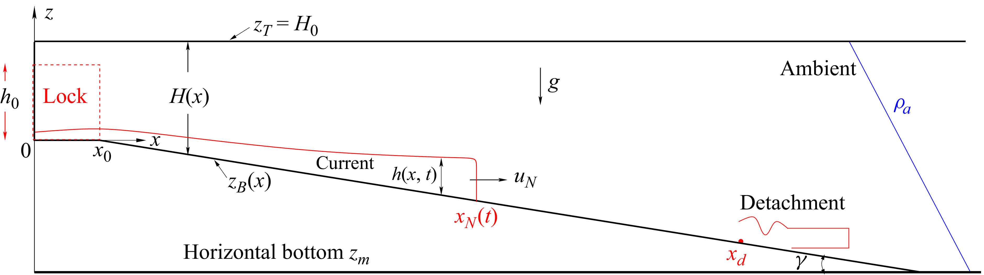
 xslope=x0
 t=0
t=0 x0,h0
x0,h0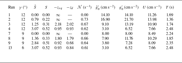
 S^,N,g^0′
 zd
zd S
S g0′
g0′ S^
S^ g^0′
g^0′ zeq
zeq ϕ=1
ϕ=1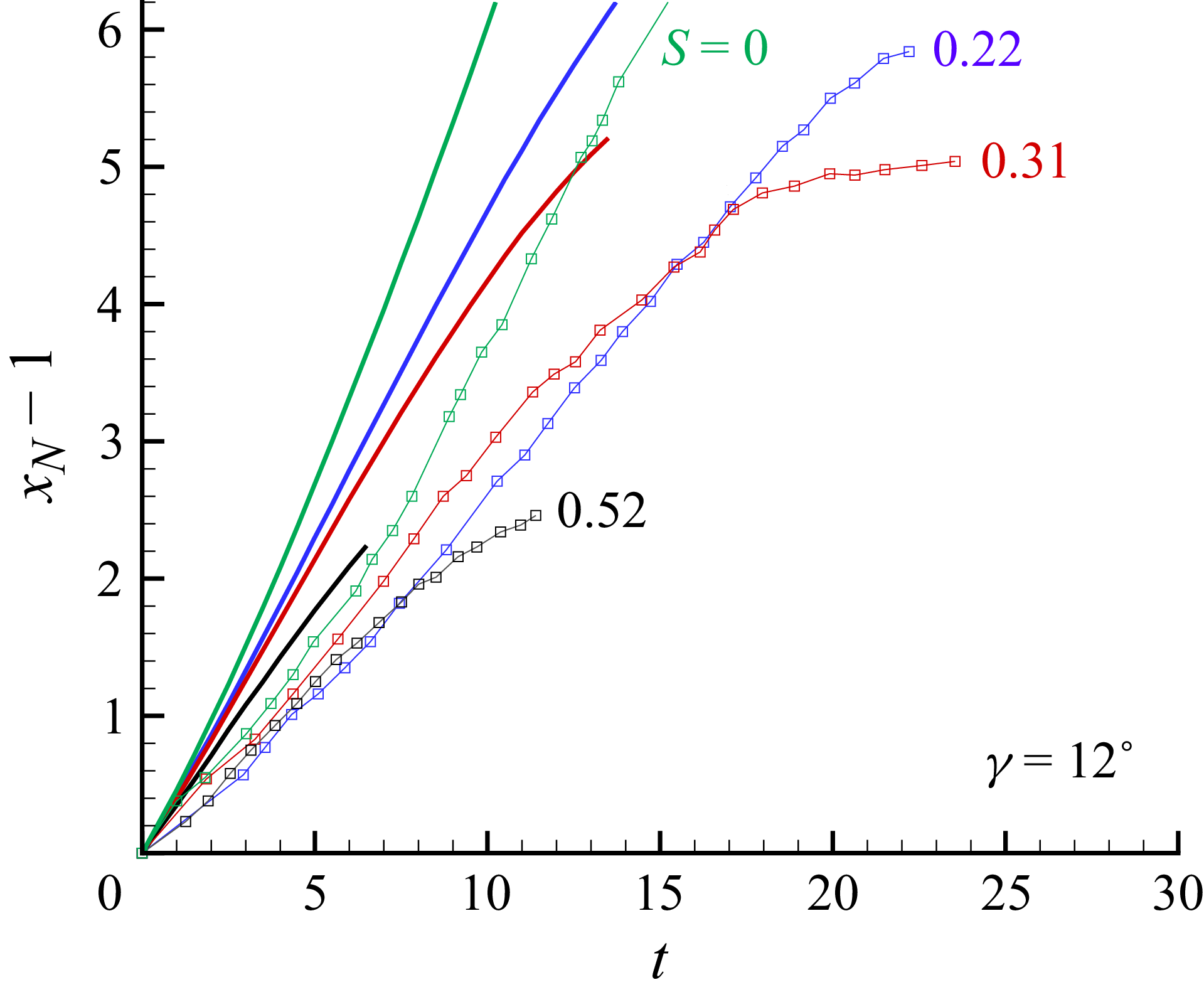
 xN−1
xN−1 t
t γ=12∘
γ=12∘ S
S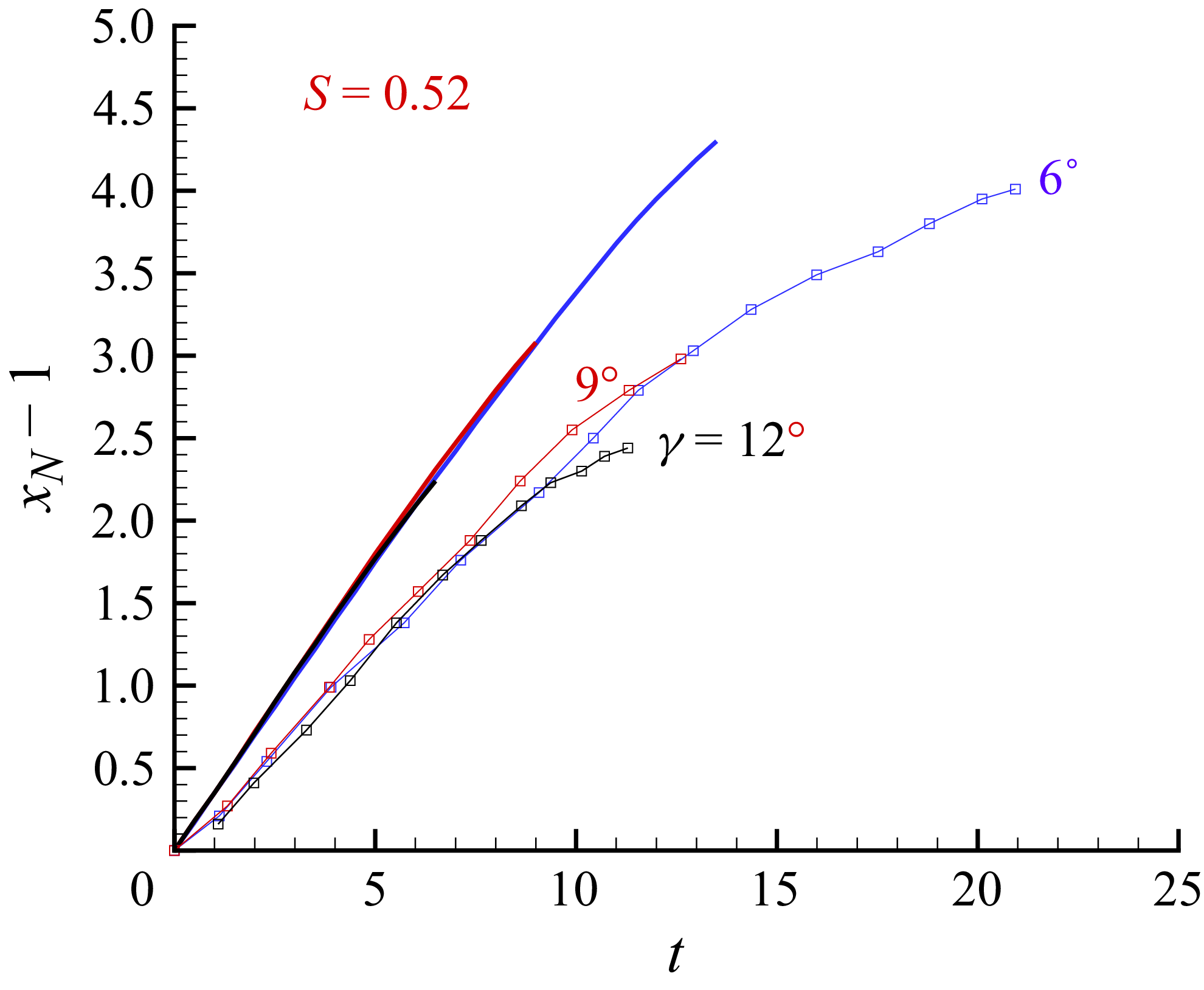
 xN−1
xN−1 t
t S=0.52
 γ
γ 6∘
6∘ 9∘
9∘ 12∘
12∘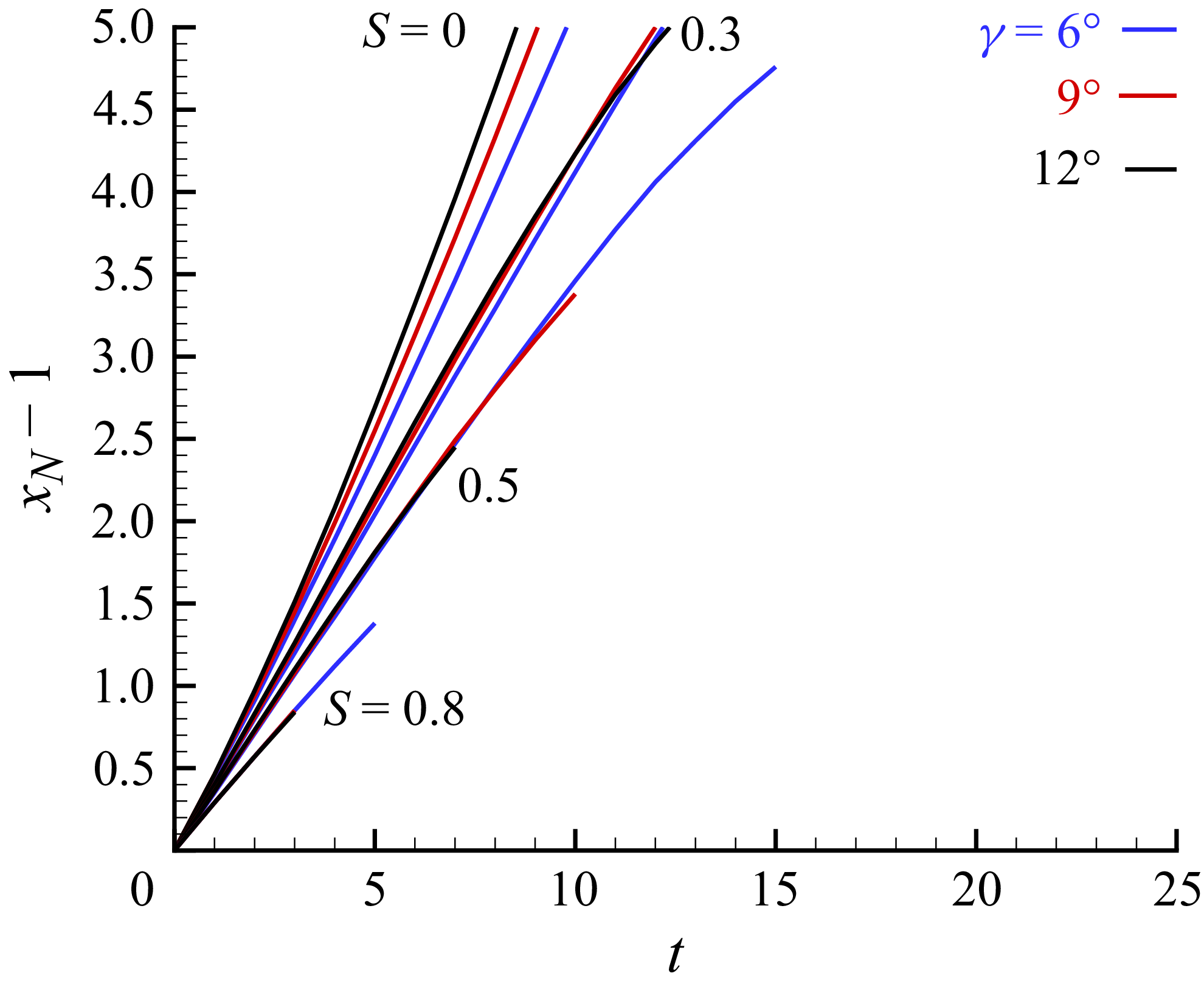
 xN−1
xN−1 t
t S=0,0.3,0.5,0.8
 γ
γ 6∘
6∘ 9∘
9∘ 12∘
12∘
 h
h x
x γ=9∘
γ=9∘ S=0.33
 S=0
S=0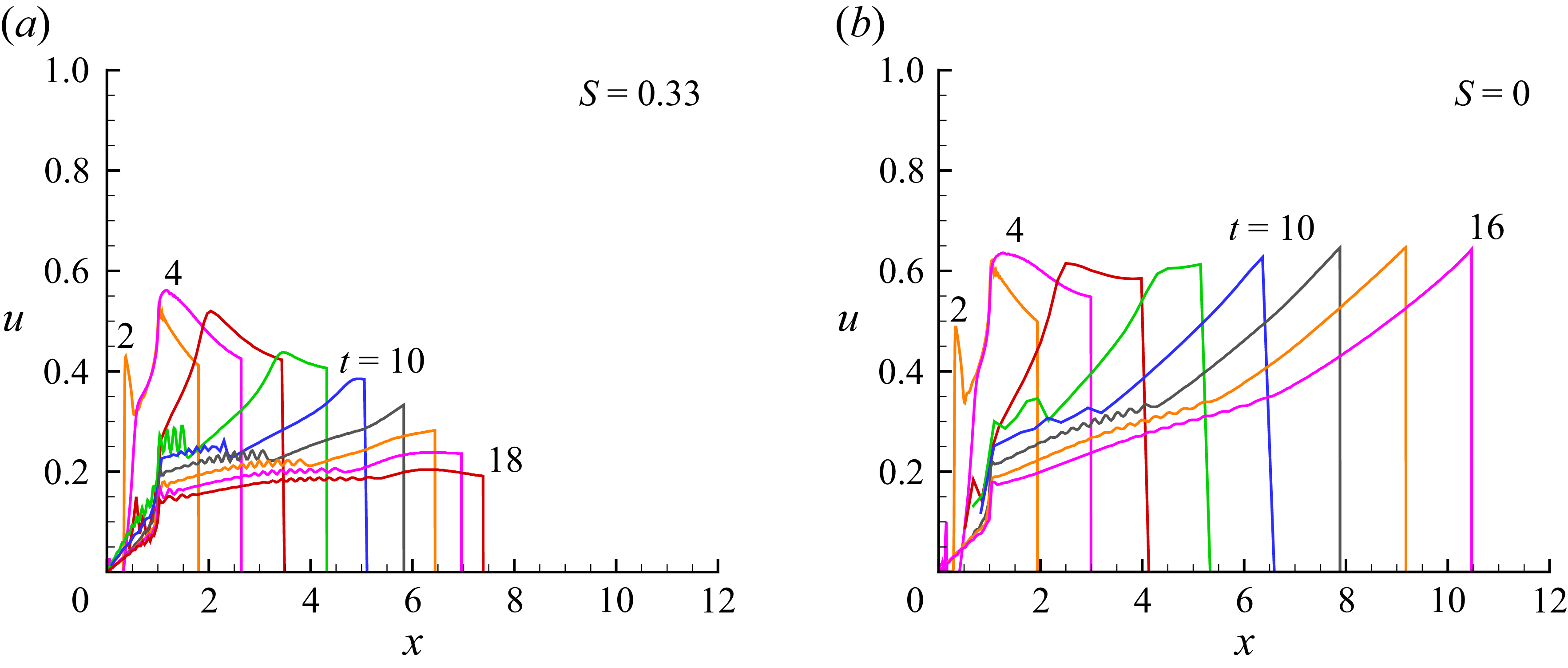
 u
u x
x γ=9∘
γ=9∘ S=0.33
 S=0
S=0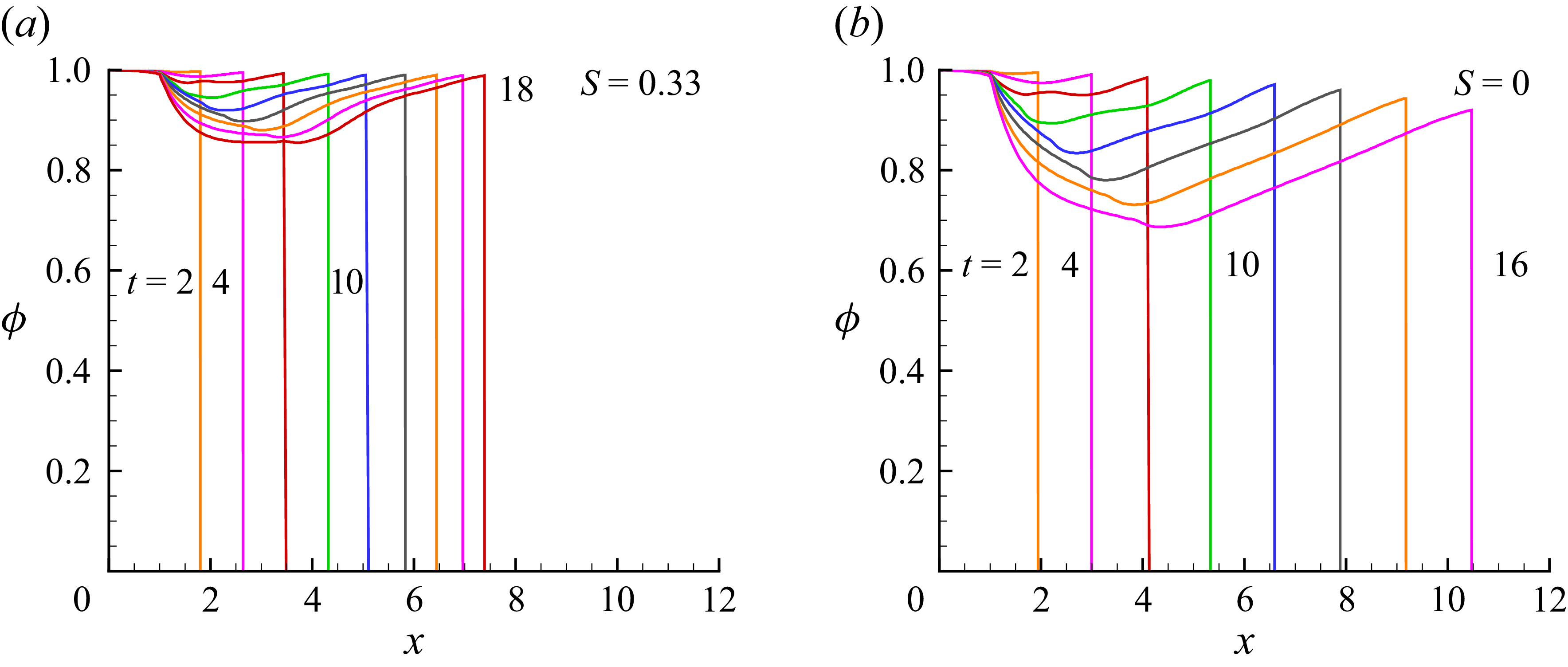
 ϕ
ϕ x
x γ=9∘
γ=9∘ S=0.33
 S=0
S=0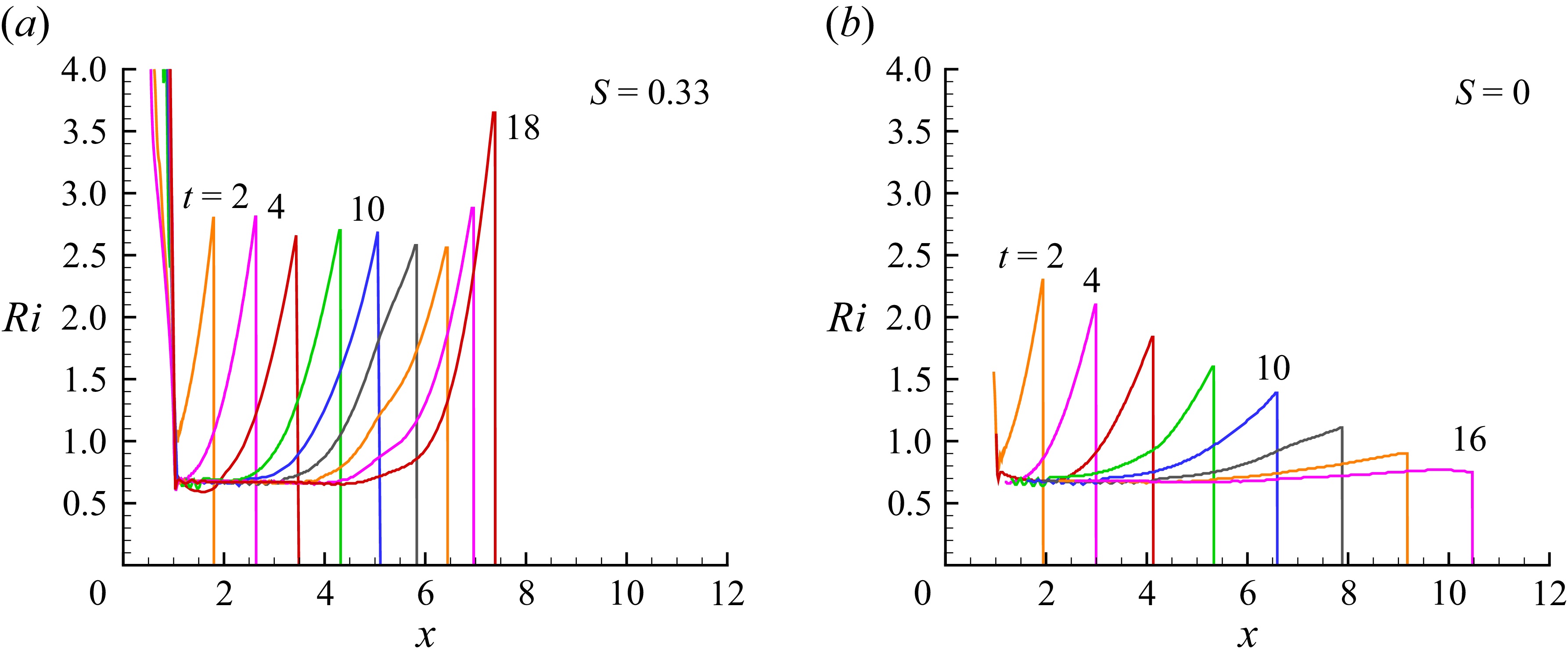
 Ri
Ri x
x γ=9∘
γ=9∘ S=0.33
 S=0
S=0
 Open access

