


1. Introduction
Neutrinos are elementary particles whose interactions with polar ice molecules can be detected from the emission of Cherenkov radiation. The Askaryan Radio Array (ARA) is a neutrino experiment at the South Pole that aims to detect high-energy neutrinos which produce coherent Cherenkov radiation in a radio-frequency band ~150 − 800 MHz (Allison and others, Reference P2012). The ARA detectors are ~150 m below the ice surface with the targeted neutrino interactions occurring at ice depths ~100–2000 m. The emitted radio waves from the ice–neutrino interaction propagate at oblique angles relative to the vertical direction with the trajectories from deeper interaction sources to the shallower detector often close to horizontal.
Characterization of the radio-frequency (bulk) permittivity of polar ice is critical to optimizing the ARA detector sensitivity and to reconstruct information about ice–neutrino interactions (Kravchenko and others, Reference Kravchenko, Besson, Ramos and Remmers2011; Allison and others, Reference Allison2019a). The real component of the permittivity relates to the volume of ice visible to the radio receiver array, whilst the imaginary component relates to the attenuation of the radio signal. Due to the presence of ice fabric – the orientation distribution of ice crystals – polar ice behaves as a birefringent medium whereby radio wave polarizations experience different permittivities and propagate at different phase velocities (Hargreaves, Reference Hargreaves1978). Characterization of ice birefringence is important for the ARA experiment as it would facilitate a range estimate from the interaction source to the detector based on polarization time delays at the ARA detectors, and subsequently aid in neutrino energy reconstruction. Measured polarization time delays using radio transmitter calibration sources have demonstrated that a significant birefringence (~0.1–0.3% of the mean refractive index) is present for oblique angle trajectories (Kravchenko and others, Reference Kravchenko, Besson, Ramos and Remmers2011; Allison and others, Reference Allison2019a). A first-principles radio propagation model that predicts the polarization time delays is, however, yet to be developed and is desirable to estimate the interaction range for an arbitrary trajectory.
Since the commencement of the ARA experiment, the SPICE (South Pole Ice Core Experiment) team have collected ice fabric data that extend down to a depth ~1750 m (Voigt, Reference Voigt2017). Ice fabric is of interest in glaciology as it indicates present stress configurations in the ice (Faria and others, Reference Faria, Weikusat and Azuma2014), and has been considered to contain information about past configurations (Alley, Reference RB1988). Additionally, changes in ice fabric are often correlated with climatic transitions (Kennedy and others, Reference Kennedy, Pettit and Prinzio2013). Polarimetric radar sounding is often used to complement direct sampling of ice fabric (Fujita and others, Reference Fujita, Maeno and Matsuoka2006; Dall, Reference Dall2010; Drews and others, Reference Drews2012; Li and others, Reference Li2018; Jordan and others, Reference Jordan, Schroeder, Castelletti, Li and Dall2019b; Brisbourne and others, Reference Brisbourne2019), and it can be used to reference azimuthal fabric orientation which is generally not recorded directly during ice coring (Wang and others, Reference Wang2002; Faria and others, Reference Faria, Freitag and Kipfstuhl2010). Terrestrial radar-sounding systems operate in a similar frequency range (~50–400 MHz) to the coherent radio-frequency emissions induced by neutrinos. Consequently, effective medium models of ice birefringence and radio propagation developed by the radar-sounding community (Fujita and others, Reference Fujita, Maeno and Matsuoka2006; Matsuoka and others, Reference Matsuoka, Wilen, Hurley and Raymond2009) are of direct relevance to understanding polarization time delays for ARA.
The focus of this study is the development of a proof-of-concept model for radio-frequency ice birefringence and polarization time delays used for range reconstruction of trajectories by the ARA experiment. In Section 2, we motivate the study by giving an overview of radio transmitter calibration by the ARA experiment, focusing on range estimation using polarization. In Section 3, we use SPICE fabric data (Voigt, Reference Voigt2017) and an effective medium framework (Fujita and others, Reference Fujita, Maeno and Matsuoka2006) to model the radio-frequency ice birefringence at the South Pole. In Section 4, we construct an oblique radio wave propagation model. In Section 5, we place model bounds upon polarization time delays and compare with new transmitter measurements from December 2018. In Section 6, we discuss the consequences of the study for neutrino source reconstruction and provide suggestions for how the modeling framework could be developed in future work.
2. Radio transmitter calibration of the ARA experiment
2.1. Overview of experiment
Neutrinos are elementary particles, which, in contrast to standard sub-atomic particles (protons, electrons, photons) interact exceedingly rarely with matter. Owing to their neutral charge, neutrinos are not deflected by magnetic fields and therefore, like photons, point directly back to their cosmic sources, motivating the growing field of neutrino astronomy. However, the ability of ultra-high-energy (UHE, ${{\cal O}}$ (1 Joule)) neutrinos to penetrate thousands of km of Earth material without interacting requires huge, uniform target volumes, such as the Antarctic ice sheet, to detect those rare interactions. Interactions of UHE neutrinos with polar ice molecules generate secondary particles which can, themselves, be detected from the Cherenkov radiation they produce.
The ARA experiment is designed to operate in the 150–800 MHz radio-frequency band, with the goal of detecting impulsive emissions from collisions of UHE extraterrestrial neutrinos with ice molecules. ARA comprises a set of five ‘receiver stations’ located within 7 km of the geographic South Pole and 5 km of the SPICE ice core located at 89°59′S, 98°9′W (refer to Fig. 1 for a plan-view schematic). Each receiver station, labeled as A1–A5, consists of two sets of near-collocated eight antennas, with eight [channels 0–7] primarily sensitive to vertical polarization (referred to as ‘v’ or ‘vpol’), and the remainder [channels 8–15] sensitive to horizontal polarization (referred to as ‘h’ or ‘hpol’). The eight vpol antennas are located at the vertices of a cuboid ~20 m on a side, and ~150 m deep into the ice. Each hpol antenna is located ~2 m vertically above each vpol antenna. Since the sensitivity is dominated by the vpol antennas, with a dipole-like cos 2θ beam pattern, and since the ice sheet is disk-like, Cherenkov radiation from neutrino interactions is typically detected at oblique arrival angles from the ice below.
Plan-view of ARA experiment at the South Pole in polar stereographic coordinate system with reference meridian 50°E. Receiver stations are indicated as squares (in various shades of red), with pulser transmitters shown in various shades of green. Particularly important to this study are the receiver stations A2 and A4, the SPICE ice core pulser (diamond, used in December 2018, with transmitter depth varying from 0 to 1200 m) and the deep pulser sources IC1S DP and IC22S DP (circles), at a fixed depth of ~1400 m. The ice flow direction is indicated and in the radio propagation model is assumed to be parallel to the x 1 axis of the fabric orientation tensor, with x 2 axis perpendicular to flow (in the horizontal plane), and the x 3 axis vertical (described in more detail in Sections 3 and 4).

As part of the initial ARA receiver calibration, three ‘deep’ radio-frequency pulsers were deployed to broadcast signals to the 1–5 km distant ARA receiver stations. The pulsers were deployed at depths typical of neutrino interactions, two at 1400 m and one at 2450 m. (The deepest pulser worked reliably for only a month after deployment, so only the two shallower pulsers, IC1S DP and IC22S DP, are indicated in Fig. 1.) Given the proximity of IC1S DP and IC22S DP (and absent any significant distinction between the experimental measurements drawn from the two pulsers), their data are combined in this study. More recently, in December 2018, a custom high-amplitude radio-frequency transmitter was lowered into the 1700 m SPICE ice core to provide additional broadcasts with a differing horizontal baseline to the pulsers.
The azimuthal orientation of the radio trajectory between the sources and receiver stations relative to the ice fabric is of particular relevance to this study. In the radio propagation model (described in detail in Sections 3 and 4), we assume that the horizontal eigenvectors of the fabric orientation tensor are aligned perpendicular and parallel to flow direction, which is 41 ± 2° with respect to Grid North (determined yearly by the National Science Foundation). The ice flow direction is also well-aligned with the horizontal extension direction, which we estimated to be 52 ± 15° with respect to Grid North from the ice surface velocity field (Rignot and others, Reference Rignot, Mouginot and Scheuchl2011, Reference Rignot, Mouginot and Scheuchl2017) following the derivative procedure in Jordan and others (Reference Jordan, Schroeder, Elsworth and Siegfried2020).
The radio trajectories from SPICE and deep pulser sources to the A2 station are approximately flow-perpendicular (azimuthal angles to flow ~77° and ~79°, respectively, for the SPICE and deep pulser sources). The radio trajectories to the A4 station are approximately flow-parallel (azimuthal angles to flow ~1° and ~18°, respectively, for the SPICE and deep pulser sources). We focus upon calibration measurements from these stations as they best represent flow-perpendicular/flow-parallel cases.
2.2. Determining the interaction range from polarization time delays
To perform neutrino astronomy, the ARA experiment must reconstruct both the energy (inferred from the measured signal amplitudes, and a knowledge of the distance and geometry relative to the neutrino interaction point) and sky source direction of the detected neutrino (from the indirect information provided by the Cherenkov radiation generated by the secondary particles produced in the neutrino interaction). Taking advantage of the three-dimensional ARA array geometry, triangulation can be used to determine the direction (azimuthal angle ϕ and elevation/polar angle θ) of the neutrino interaction point in the ice. Determining the range to the neutrino interaction point is, however, considerably more challenging. To address this challenge, measurement of the polarization time delay between h and v polarizations at the ARA detectors has been proposed (Kravchenko and others, Reference Kravchenko, Besson, Ramos and Remmers2011; Allison and others, Reference Allison2019a). In turn, combined with the information on ice birefringence, this polarization time delay can then be converted into a range-to-neutrino vertex.
The ARA collaboration has previously reported h-v time delays for data taken using the deep pulser sources IC1S DP and IC22S DP and the SPICE icehole pulser (Allison and others, Reference Allison2019a, Reference Allison2019b; Jordan and others, Reference Jordan and Latif2019a). These results are summarized quantitatively in Section 5.1. It is observed that there are significant differences in h-v time delays for A2 and A4 stations. This occurs, despite the stations having comparable horizontal baselines (~2300 and 3200 m for SPICE to A2 and SPICE to A4, and ~3700 m, in each case, for broadcasts from the deep pulsers). Understanding the asymmetry to the polarization time delay, and how it relates to ice birefringence and range estimation, provides the motivation for the radio propagation model developed in this study.
3. Modeling ice birefringence
3.1. Effective medium model
At radio frequencies, the bulk dielectric tensor, principal refractive indices and birefringence of polar ice can be modeled by combining ice fabric measurements (the c-axis orientation distribution) with information about the birefringence of individual ice crystals (Fujita and others, Reference Fujita, Maeno and Matsuoka2006; Matsuoka and others, Reference Matsuoka, Wilen, Hurley and Raymond2009). This effective medium approach was developed to interpret polarimetric radar sounding measurements (Fujita and others, Reference Fujita, Maeno and Matsuoka2006; Matsuoka and others, Reference Matsuoka, Power, Fujita and Raymond2012; Brisbourne and others, Reference Brisbourne2019; Jordan and others, Reference Jordan, Schroeder, Castelletti, Li and Dall2019b) and assumes that the dimensions of the ice crystal grains (~mm) are much less than radio wavelength in ice (~dm-m for the frequency-range relevant to ARA).
Individual ice crystals have a hexagonal structure and are uniaxially birefringent with the optic axis aligned with the crystallographic axis (c-axis) (Hargreaves, Reference Hargreaves1978). The magnitude of the crystal birefringence (in terms of the permittivity) is given by ${\Delta \epsilon }'={\lpar \epsilon _{\parallel c}-\epsilon _{\bot c}\rpar }$ where $\epsilon _{\parallel c}$
 and ε⊥c are the relative principal permittivities parallel and perpendicular to the c-axis, respectively, with $\epsilon _{\parallel c}\gt \epsilon _{\bot c}$
 (Fujita and others, Reference Fujita, Matsuoka, Ishida, Matsuoka and Mae2000). (The notation Δε′ is used as the radar sounding literature normally uses Δε for the bulk birefringence.) At radio frequencies and as ice temperature increases from − 60° → 0 C, Δε′ increases by ~5% from ~ 0.0325 → 0.0345 (Matsuoka and others, Reference Matsuoka, Fujita and Mae1996; Fujita and others, Reference Fujita, Matsuoka, Ishida, Matsuoka and Mae2000).
Ice fabric measurements consist of thin ice core sections that measure the ice crystal orientation distribution in terms of a second-order orientation tensor (Woodcock, Reference Woodcock1977; Montagnat and others, Reference Montagnat2014). The orientation tensor represents the c-axis orientation distribution as an ellipsoid where the eigenvalues, E 1, E 2, E 3 represent the relative c-axis concentration along each principal coordinate direction, x 1, x 2, x 3. The eigenvalues have the property E 1 + E 2 + E 3 = 1, and following the radar polarimetry convention, we assume E 3 > E 2 > E 1. Using this eigenvalue framework, the bulk principal dielectric tensor is given by

(Fujita and others, Reference Fujita, Maeno and Matsuoka2006). For the general case, (E 1 ≠ E 2 ≠ E 3), polar ice therefore behaves as a biaxial medium (three different principal permittivities). The principal refractive indices, which correspond to the axes of the biaxial indicatrix ellipsoid, are given by


Matsuoka and others (Reference Matsuoka, Wilen, Hurley and Raymond2009) further discuss the biaxial indicatrix representation, and how it relates to different propagation directions in radar sounding.
The ice fabric depends on the stress regimes present in ice sheet. Due to ice viscosity being an order of magnitude higher parallel to the c-axis than perpendicular, aggregates of ice crystals tend to align toward the compression axis and away from the extension axis (Alley, Reference RB1988). End-member classes used to describe ice fabrics are: ‘random/isotropic’ ($E_{1}\approx E_{2} \approx E_{3} \approx {1\over 3}$ and associated with the near-surface), ‘single-pole’ (E 1 ≈ E 2 ≈ 0, E 3 ≈ 1 and associated with deeper ice undergoing vertical compression), and ‘vertical girdle’ ($E_{1} \approx 0\comma\; E_{2} \approx E_{3}\approx {1\over 2}$
 and associated with lateral tension).
3.2. Principal refractive index profiles from the SPICE ice core
Figure 2 shows fabric eigenvalue profiles from the SPICE ice core with samples taken at ~20 m intervals (Voigt, Reference Voigt2017). The plot indicates development from a relatively random fabric in shallower ice (E 3 ≈ 0.45, E 2 ≈ 0.30, E 1 ≈ 0.25 at z = 150 m) to a vertical girdle fabric in deeper ice (E 3 ≈ 0.50, E 2 ≈ 0.49, E 1 ≈ 0.01 at z = 1750 m). Profiles for the principal refractive indices, calculated as above with ε⊥=3.157 and Δε′ = 0.034 (corresponding to a polarization-averaged refractive index $\bar {n} = 1.78$ ), are shown on the right axis of Figure 2.
Left axis: fabric eigenvalues from the SPICE ice core (Voigt, Reference Voigt2017). Right axis: eigenvalues translated into principal refractive indices.
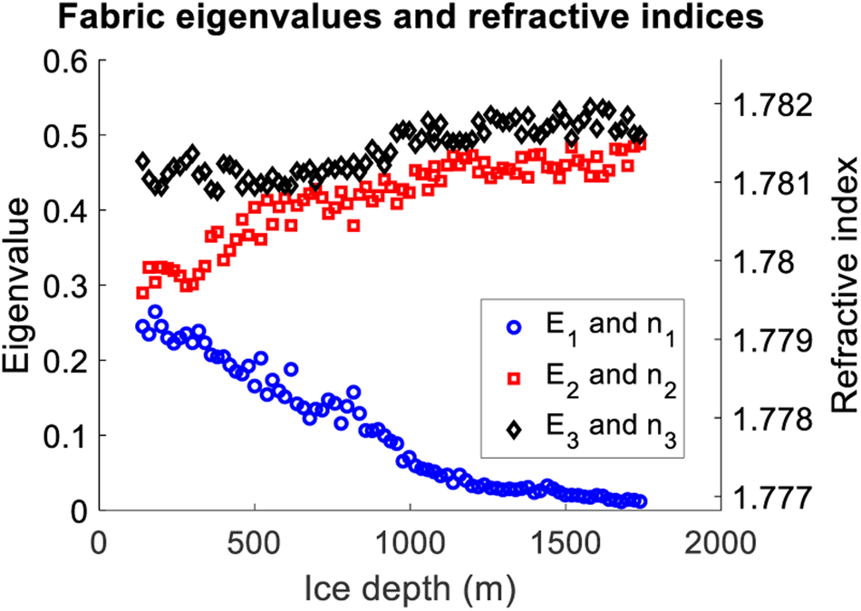
Due to the dominance of vertical compression, the x 3 axis (greatest c-axis concentration) is generally close to being aligned with the vertical (Matsuoka and others, Reference Matsuoka, Wilen, Hurley and Raymond2009), and is typically approximated as vertical in polarimetric radar sounding studies (Fujita and others, Reference Fujita, Maeno and Matsuoka2006; Brisbourne and others, Reference Brisbourne2019; Jordan and others, Reference Jordan, Schroeder, Castelletti, Li and Dall2019b). Since the azimuthal orientation of the ice core fabric sections are not recorded during drilling, the x 1 and x 2 directions are not initially known. For an ice flow model where there is a lateral component of tension present, the x 2 axis (greatest c-axis concentration in horizontal plane) is expected to be approximately perpendicular to the horizontal extension direction (shown to align with the ice flow direction in Section 2), with the x 1 axis parallel (Wang and others, Reference Wang2002; Fujita and others, Reference Fujita, Maeno and Matsuoka2006). Using polarimetric radar sounding, this predicted behavior has been verified at ice divides such as the NEEM ice core region in northern Greenland (Dall, Reference Dall2010; Jordan and others, Reference Jordan, Schroeder, Castelletti, Li and Dall2019b).
4. Modeling oblique radio wave propagation
In the radio propagation model, we assume that the ice sheet can be modeled as a stratified anisotropic medium. Each layer of the ice sheet has thickness δz i which is determined from the vertical spacing of the SPICE ice core eigenvalue data (~20 m). The dielectric properties of each layer are defined by the dielectric tensor, Eqn (1), corresponding to the principal refractive indices, Eqn (4). Lacking information about the azimuthal fabric orientation, in the model description, we assume the ‘conventional’ fabric orientation described in Section 3.2, with the x 3 axis vertical, the x 2 axis perpendicular to flow and the x 1 axis parallel to flow.
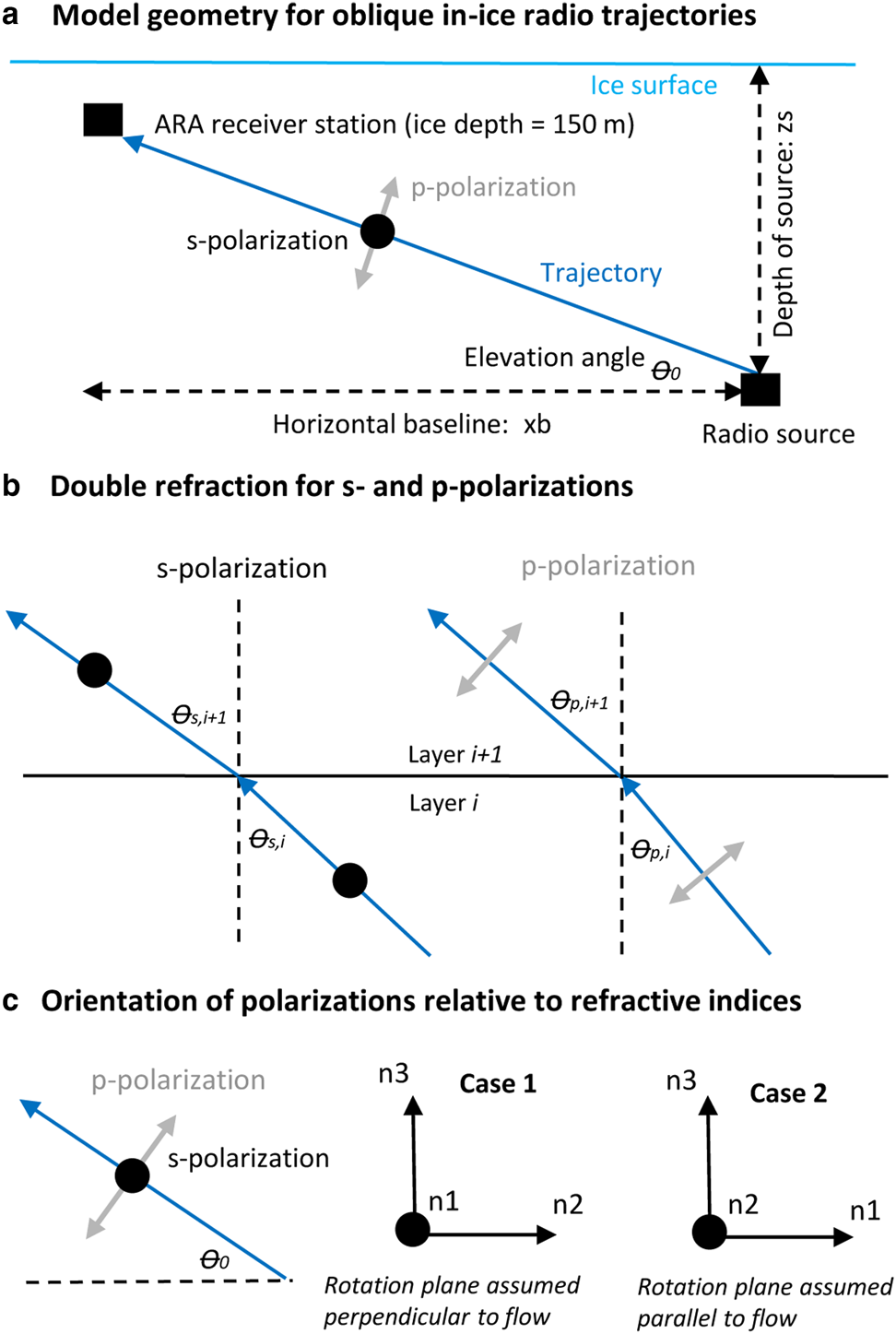
The radio propagation model is formulated for s- and p-polarizations (electric field perpendicular and parallel to the incidence plane, respectively). A schematic of the model geometry assuming a straight-line trajectory is shown in Figure 3(a). In each layer the s- and p-polarizations have different refractive indices and follow separate trajectories following Snell's law shown in the schematic in Figure 3(b). The model considers two bounding scenarios: (i) where the wave propagation vector is assumed to be in the x 2x 3 plane (and therefore the trajectory is ‘perpendicular to flow’ when viewed from above), (ii) where the wave propagation vector is assumed to be in the x 1x 3 plane (and therefore the trajectory is ‘parallel to flow’ when viewed from above). The principal refractive indices in relation to model geometry are shown in Figure 3(c). For these restricted propagation directions, the s- and p-polarizations propagate along independent paths within the ice sheet and a double refraction/ray propagation model can be used.
(a) Geometry for oblique radio propagation model. The black circles indicate that the s-polarization oscillates in the plane perpendicular to the radio trajectory. (b) Schematic showing double refraction for s- and p-polarizations in adjacent layers of the ice sheet (the differences in refraction angles are exaggerated). (c) Orientation of principal refractive indices in relation to model geometry for the two bounding cases considered where case 1 corresponds to propagation in the x 2x 3 plane and case 2 corresponds to propagation in the x 1x 3 plane. The model assumes that the E 3 eigenvector is vertical, the E 2 eigenvector is perpendicular to flow and the E 1 eigenvector is parallel to flow.
This model approach is analogous to modeling oblique propagation within birefringent optical reflectors (Weber and others, Reference Weber, Stover, Gilbert, Nevitt and Ouderkirk2000; Orfanidis, Reference Orfanidis2016). Computationally, the model is set-up with the source depth and the horizontal baseline fixed with sin(θp,i) and sin(θs,i) as degrees of freedom to be solved for subject to Snell's law being satisfied in each layer. The model is equivalent to Fermat's least time principle being satisfied separately by each polarization mode.
For propagation in the x 2x 3 plane, the s- and p-polarization refractive indices of the ith layer are given by


where the first subscript indicates the principal refractive index component with θp,i the p-polarization propagation angle in the ith layer (Matsuoka and others, Reference Matsuoka, Wilen, Hurley and Raymond2009; Orfanidis, Reference Orfanidis2016). For propagation in the x 2x 3 plane, the 1 and 2 subscripts are interchanged between Eqns (6) and (5). The propagation angles in each layer are derived from separate applications of Snell's law:
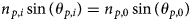

where θ s,i is the s-polarization propagation angle in the ith layer and the subscript 0 indicates the source layer. (In a multilayer optical structure, it is sufficient to apply Snell's law with respect to the source layer, rather than adjacent layers.) Orfanidis (Reference Orfanidis2016) provides analytical expressions for θ p,i in terms of the principal refractive indices that were used in the model code. The deviation between θ s,i and θ p,i from a straight-line trajectory increases with the angle of incidence, with the highest angular offset in our simulation domain ~ 0.2°.
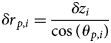
The radio propagation model enables calculation of the s-p signal arrival time delay for propagation in the planes of the principal axes, which serve as bounding cases for the observed h-v time delays at the receiver stations. In each layer of the ice sheet, the radio path lengths are given by

which corresponds to layer time increments


and the total s-p time delay is then given by

When ΔT s,p < 0 the s-polarization arrives at the detector before the p-polarization.
It is straightforward to understand why the two propagation scenarios (Fig. 3(c)) represent bounds on ΔT s,p for a given azimuthal trajectory angle. For case 1 (assumed flow-perpendicular) the s-p birefringence, n s,i − n p,i and ΔT s,p are both minimized. This follows from the s-polarization being aligned with n 1 (the lowest possible horizontal refractive index) and the horizontal component of the p-polarization being aligned with n 2 (the greatest possible contribution to n p from the horizontal direction). For case 2 (assumed flow-parallel), n s,i − n p,i and ΔT s,p are both maximized as the reverse orientation occurs. The general case of azimuthal trajectory angle (not modeled in this study) is anticipated to have values for ΔT s,p between these bounding cases.
The model uncertainty for ΔT s,p arises due to uncertainty in n s,i − n p,i which, in turn, relates to measurement uncertainty in the fabric eigenvalues and crystal birefringence in Eqns (2)–(4). Following a Taylor expansion of Eqn (2) and (3), it can be shown that the refractive index birefringence scales as n 2 − n 1 ≈ $\Delta \epsilon '\lpar E_{2}-E_{1}\rpar /2\sqrt \epsilon _{\bot c}$ (and so on for the other index combinations). Due to the product form, the fractional uncertainty in Δε′, $\sqrt \epsilon _{\bot c}$
 , E 1 and E 2 propagate in quadrature for the uncertainty on n 2 − n 1. Based on Greenland ice core data (Montagnat and others, Reference Montagnat2014), we assume an uncertainty in the fabric eigenvalues ±0.03 (corresponding to a fractional uncertainty ${\sim}10\percnt$
 ). The fractional uncertainty for ε′ and ε⊥c are approximately an order of magnitude smaller (Fujita and others, Reference Fujita, Matsuoka, Ishida, Matsuoka and Mae2000, Reference Fujita, Maeno and Matsuoka2006) and hence are neglected in the analysis. Uncertainties were incorporated in the simulations assuming normally distributed random variables for E 1, E 2 and E 3 and then measuring the standard deviation of the ensemble for ΔT s,p.
5. Results
5.1. Polarization time delay measurements
We now present polarization time delay measurements from the radio transmitter calibration sources previously described in Section 2. Using data for the vpol channels (0–7) versus the hpol channels (8–15) we fitted the distributions for the h-v polarization time delay ΔT h,v (defined analogously to ΔT s,p in Eqn (13)) to Gaussian signal shapes. The results of fits that converged and also had an acceptable χ2 are presented in Table 1. We note the clear offset between the most-probable signal arrival time differences for the A2 station (significant negative h-v time delays with ΔT h,v < −13 ns for the SPICE transmitter and ΔT h,v < −24 ns for the deep pulser transmitters) versus the A4 station (generally negligible h-v time delays).
Results of Gaussian fits to ΔT h,v distributions for v-h doublets, in units of nanoseconds. Due to their very similar trajectories, broadcasts from the deep pulser sources, IC1S DP and IC22S DP, are grouped together. The horizontal baselines are x b = 2353 m (SPICE → A2), x b = 3702 m (SPICE → A4), x b = 3199 m (mean for deep pulser → A2) and x b = 3700 m (mean for deep pulser → A4). ΔT h,v < 0 corresponds to the h-polarization signal arrival at the receiver station before the v-polarization

5.2. Model simulations for ice birefringence and polarization time delays
To understand the origin of the polarization time delay asymmetry in Table 1, we now evaluate the radio propagation model as a function of horizontal baseline and source depth. Figures 4(a) and (c) show modeled s-p time delays perpendicular and parallel to ice flow (based on our model assumption that the principal coordinates are also aligned perpendicular and parallel to flow). For the flow-perpendicular case, ΔT s,p is always negative and increases with both ice depth and horizontal baseline. For the flow-parallel case, ΔT s,p switches sign from positive to negative at incidence angle ~ 65 − 70°. |ΔT s,p| is always greater for the flow-perpendicular case than the flow-parallel case.
(a) Polarization time delay for flow-perpendicular trajectories (case 1). (b) Path-averaged birefringence for flow-perpendicular trajectories. (c) Polarization time delay for flow-parallel trajectories (case 2). (d) Path-averaged birefringence for flow-parallel trajectories. (e) Elevation/polar propagation angle for straight-line trajectory. The model assumes that the E 3 eigenvector is vertical, the E 2 eigenvector is perpendicular to ice flow and the E 1 eigenvector is parallel to ice flow.
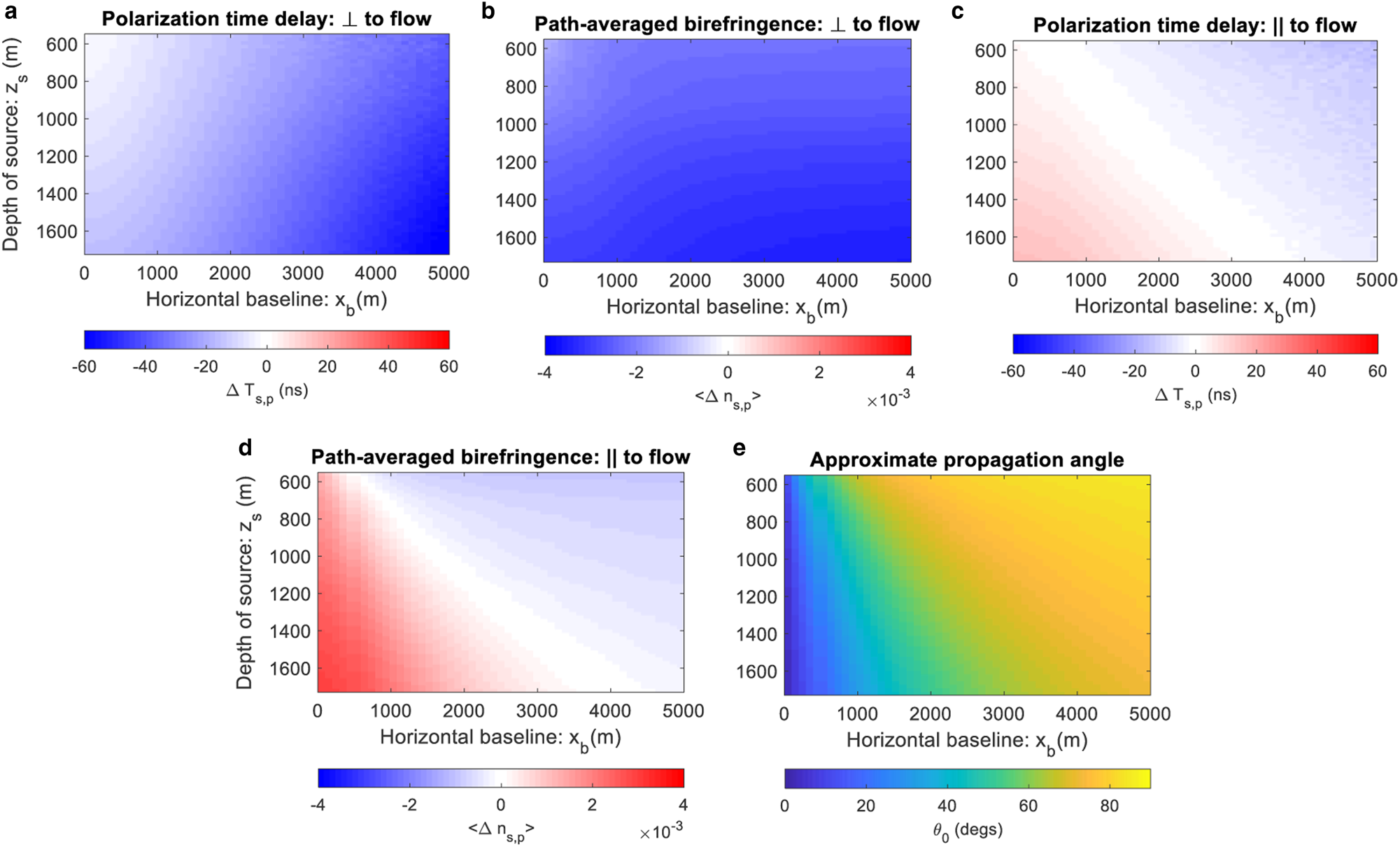
There is a simple explanation for the relationships in Figures 4(a) and (c) in terms of the path-averaged s-p birefringence, 〈Δn s,p〉 = 〈n s − n p〉, where 〈…〉 denotes ‘path-averaged’. Plots for 〈Δn s,p〉 are shown in Figures 4(b) and (d), with the incidence angle for a straight-line trajectory shown in Figure 4(e). In the flow-perpendicular case, since n 1 < n 2 < n 3, it follows that 〈Δn s,p〉 < 0 and ΔT s,p < 0 hold for all angles of incidence. In the flow-parallel case, 〈Δn s,p〉 switches sign from positive to negative at the same incidence angle where ΔT s,p switches sign. Conceptually, this transition behavior occurs as the p-polarization refractive index, Eqn (5), is dominated by the n 3 component for oblique angles and n 1 for shallow angles. At normal incidence (x b = 0), and 〈Δn s,p〉 for the flow-perpendicular case equals − 〈Δn s,p〉 for the flow-parallel case.
Previous analysis of ice birefringence at the South Pole has been discussed in terms of fractional ‘birefringent asymmetry’ (Kravchenko and others, Reference Kravchenko, Besson, Ramos and Remmers2011; Allison and others, Reference Allison2019a) which can be estimated via the ratio $\vert \langle \Delta n_{s\comma p}\rangle \vert /\bar {n}$ where $\bar {n}=1.78$
 is the mean refractive index. Figure 4 shows that for flow-perpendicular case |〈Δn s,p〉| ranges from 0.02 to 0.035, which corresponds to $\vert \langle \Delta n_{s\comma p}\rangle \vert /\bar {n} \sim 0.11 - 0.20\percnt$
 .
.
The propagated uncertainty for ΔT s,p (based on the spread of a model ensemble assuming eigenvalue uncertainty of ±0.03) is less than 1 ns, and typically ~0.5 ns. As this is small, we do not show this in Figure 4 or the following figures.
5.3. Model simulations for range estimation
In the ARA experiment, the elevation/polar and azimuthal angles of a trajectory are constrained interferometrically, with the interaction range (i.e. the distance along a trajectory for specified elevation and azimuth) the major unknown. Figure 5 compares the relationship between modeled polarization time delay and range for the flow-perpendicular and flow-parallel cases for three fixed elevation angles. This figure represents a hypothetical scenario where the azimuthal angles of the trajectories are known a-priori to be aligned with the principal coordinate system.
Modeled polarization time delay versus range for: (a) flow-perpendicular (case 1) and (b) flow-parallel (case 2) trajectories for three polar/elevation angles. The curves are different lengths as the maximum depth and range is fixed by the depth of the SPICE ice core fabric measurements.
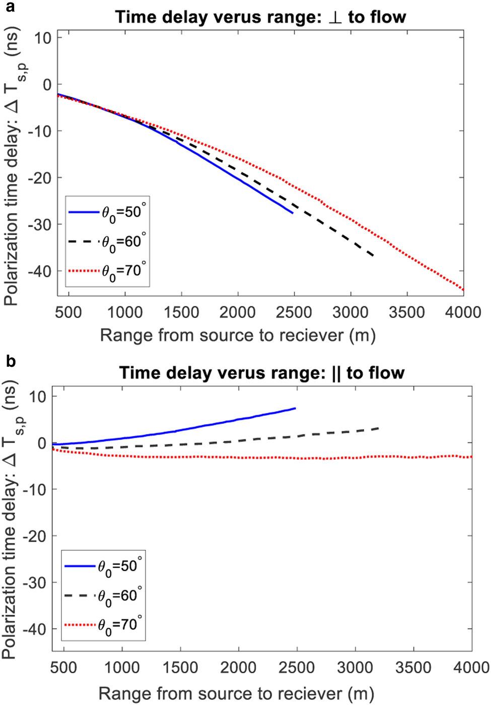
For the flow-perpendicular scenario, at all elevation angles, there is a monotonic negative relationship between the range and the polarization time delay. For the flow-parallel scenario, there is significantly less variation in the polarization time delay as a function of range, with the polarization time delay approximately constant for θ0 = 70°. As in Figures 4(a) and (c), these results can be related to the path-averaged s-p birefringence in Figures 4(b) and (d).
5.4. Model-data comparison
The modeled s-p time delays are compared with measured h-v time delays from the A2 and A4 stations (mean and rms deviation averaged over all channels in Table 1) respectively in Figure 6. The model simulations in the comparison assume equivalent horizontal baselines to the data. The purpose of the comparison is not to demonstrate precise quantitative agreement (primarily since the A2 and A4 stations are not precisely aligned with the flow as is assumed in the model). Instead, the purpose is to check for qualitative agreement, and assess the validity of our assumption regarding fabric orientation relative to the ice flow direction. It is also to be noted that the modeled p-polarization is not strictly equivalent to the measured v-polarization. In general, the p-polarization consists of horizontal and vertical components, becoming solely vertical at glancing incidence (Fig. 3). However, the trajectories in the model-data comparison (Fig. 6) are highly oblique with the smallest angle of incidence ~70°.
Model-data comparison between s-p and h-v polarization time delays. The model assumes that the SPICE → A2 and deep pulser → A2 trajectories are perpendicular to ice flow (model case 1) with baselines x b = 2353 m, x b = 3702 m and the SPICE → A4 and deep pulser → A4 trajectories parallel to ice flow with baselines x b = 3199 m, x b = 3700 m (model case 2). The measurements are azimuthally offset from ice flow as described in Section 2.

For the flow-perpendicular case, the mean measured time delays are ΔT h,v = −14.1 ± 2.8 ns (SPICE → A2 trajectory) and ΔT h,v = −25.2 ± 2.0 ns (deep pulser → A2 trajectory) with modeled time delays ΔT s,p = −22.3 and − 41.8 ns, respectively. For flow-parallel case, the measured time delays are ΔT h,v = 4.6 ± 9 ns (SPICE → A4 trajectory) and ΔT h,v = 0.7 ± 1.4 ns (deep pulser $\to$ A4 trajectory) with modeled time delays ΔT s,p = −5.8 and ΔT s,p = −3.9 ns, respectively.
Qualitatively, the model-data comparison for flow-perpendicular/A2 in Figure 6 is consistent with the modeling ansatz that the E 2 eigenvector (greatest horizontal c-axis concentration) is perpendicular to the ice flow direction and unchanging with ice depth. In particular, the measured time delays are smaller in magnitude than the modeled bound, which is consistent with the A2 measurements having an azimuthal orientation that is offset from the fabric eigenvectors. In turn, this is qualitatively consistent with our modeling ansatz, as A2 has an azimuthal orientation > 10° from the flow direction. Qualitatively the model-data comparison for flow-parallel/A4 is not fully consistent with the model bounds as the error bounds for the measured time delays are slightly greater than the modeled time delay (which represents an upper bound for the simple radio propagation model that was assumed).
6. Discussion
6.1. Implications for neutrino interaction range estimation
The radio propagation model developed in this study confirms prior observations (Allison and others, Reference Allison2019a, Reference Allisonb) that long-baseline radio-frequency trajectories measured by ARA have a polarization time delay asymmetry present. Specifically, modeling in Figures 5–6 and measurements in Table 1 indicate that there is a significant time delay for trajectories that are aligned perpendicular (or near-perpendicular) to the ice-flow direction, but not parallel. For the flow-perpendicular case, modeling and measurements also demonstrate that the magnitude of the polarization time delay increases with horizontal baseline and with interaction range (refer to Allison and others (Reference Allison2019b) Figures 14 and 15 for measurements of the range relationship).
The radio propagation model was introduced as a bounding case with the (assumed) flow-perpendicular and parallel trajectories corresponding to minimum and maximum time delays. Figure 5(a) therefore places a bound on the minimum range that can be estimated from a given measured polarization time delay (corresponding to the case where the trajectory is precisely flow-perpendicular, and the azimuthal fabric orientation is fixed with ice depth). However, to be useful in practice (and even if the idealized model assumptions about orientation were correct) the model result in Figure 5(a) would need to be generalized for a range of azimuthal trajectories. Figure 5(b) confirms that range estimation is highly unlikely to be successful for trajectories near-parallel to the ice-flow direction, with the modeled polarization time delay typically comparable to an experimental error in Table 1.
6.2. Comparison with previous measurements
Our modeled time delay at normal incidence (Fig. 4(a) and (c)) can be compared with previous measurements by Kravchenko and others (Reference Kravchenko, Besson, Ramos and Remmers2011). Specifically, as part of the RICE (Radio Ice Cerenkov Experiment) particle astrophysics experiment, Kravchenko and others (Reference Kravchenko, Besson, Ramos and Remmers2011) measured a ~50 ns time delay for the bed echo from co-polarized antennas orientated perpendicular and parallel to flow at the ice surface. We can estimate the two-way time delay between the deepest SPICE fabric measurement at 1740 m and the ice bed at 2800 m to be ~18 ns (which follows from converting a one-way time delay of ~16 ns at 1740 m in Fig. 4(a) and (c). From this additional time delay, we can then estimate the path-averaged birefringence in deeper ice (between 1740 and 2800 m) to be 〈n 2 − n 1〉 ~ 0.0025 and the path-averaged horizontal eigenvalue difference (girdle strength) to be 〈E 2 − E 1〉 ~ 0.26. The estimate for 〈E 2 − E 1〉 in deeper ice is therefore consistent with a depth-transition between a vertical girdle and single maximum fabric, which is a common feature in other ice cores (e.g. Montagnat and others (Reference Montagnat2014)).
6.3. Future development of the radio propagation model
In the development of an improved radio propagation model (that estimates the range for a given azimuth, elevation angle and time delay), it is highly desirable to have better constraints on azimuthal fabric orientation. This is a goal that the ice-core drilling community have been working toward (Hvidberg and others, Reference Hvidberg, Steffensen, Clausen, Shoji and Kipfstuhl2002; Weikusat and others, Reference Weikusat2017). In the absence of ice-core data, azimuthal constraints on fabric orientation could be established using polarimetric radar-sounding measurements from the ice surface (e.g. Fujita and others, Reference Fujita, Maeno and Matsuoka2006; Jordan and others, Reference Jordan, Schroeder, Castelletti, Li and Dall2019b) in conjunction with calibration using polarization time delay data from all five ARA receiver stations.
As it stands, a key limitation of the radio propagation model is that it is only valid for incidence planes which contain the principal axes, which results in the s- and p-polarizations propagating as independent modes through the ice sheet. A more general propagation model, formulated for a general propagation direction relative to the principal axis system, would result in wave-splitting and a coupling of the polarization modes. This mode-coupling behavior could potentially be modeled by adapting a Jones matrix model for nadir radio propagation (Fujita and others, Reference Fujita, Maeno and Matsuoka2006) for oblique radio propagation. Another key limitation of the model is that we assume that the fabric eigenvectors are precisely aligned perpendicular and parallel to flow and are unchanging with ice depth. Whilst the model-data comparison is broadly consistent with this assumption, there is likely to be at least some deviation from this idealized behavior.
7. Summary and conclusions
In this study, we used ice fabric data from the SPICE ice core to model radio-frequency ice birefringence and its effect upon oblique radio wave propagation relevant to in-ice neutrino detection at the ARA. The model framework enabled us to consider bounding cases for polarization time delays across the array (trajectories perpendicular and parallel to ice flow assuming alignment with the eigenvectors of the fabric orientation tensor), with a view to placing constraints upon range reconstruction for in-ice neutrino interactions. We then compared the modeled time delays with radio transmitter measurements and demonstrated that significant polarization time delays occur for trajectories perpendicular, but not parallel, to the ice flow direction. This result can be understood from the polarization-dependent refractive indices that are modeled from the ice core fabric eigenvalue data.
The model demonstrated that, for flow-perpendicular trajectories, there is a monotonic relationship between the polarization time delay and the trajectory range. Hence, when combined with information on ray inclination, this study raises the possibility that ice birefringence can be used to constrain the range to a neutrino interaction for trajectories near-perpendicular to ice flow. However, better constraints on azimuthal fabric orientation, and development of a more general radio propagation model, are desirable for quantitative range estimation.
Acknowledgments
We thank two anonymous reviewers and our editor, Olaf Eisen, for their valuable comments. TMJ would like to acknowledge the support from EU Horizons 2020 grant 747336-BRISRES-H2020-MSCA-IF-2016. DZB and AN acknowledge support from the MEPhI Academic Excellence Project (Contract No. 02.a03.21.0005) and the Megagrant 2013 program of Russia, via agreement 14.12.31.0006 from 24.06.2013.


 Open access