2.1. Governing equations and thermodynamics

In this study, we use the compressible Euler equations as a model for the fluid dynamics of both the liquid and gas phases. In one dimension, these are shown in their conservation form as

(2.1) \begin{equation} \frac{\partial \boldsymbol{U}}{\partial t} + \frac{\partial}{\partial x}\boldsymbol{F}(\boldsymbol{U}) = 0, \end{equation}

where $\boldsymbol {U} = (\rho, \rho u, E )^{\rm T}$ denotes the vector of conserved variables, and $\boldsymbol {F}(\boldsymbol {U}) = (\rho u,$ $\rho u^2 + p, u(E + p ) )^{\rm T}$ denotes the flux vector. In the above, $\rho$ denotes the density, $u$ is the velocity, and $p$ is the pressure. The total energy $E$, defined as the sum of the kinetic and internal energies, is

(2.2) \begin{equation} E = \rho(\tfrac{1}{2}u^2 + e), \end{equation}

where $e$ denotes the specific internal energy. To close the equations, we also require an equation of state. In this study, the stiffened gas equation of state (SG EoS) is adopted (Menikoff & Plohr Reference Menikoff and Plohr1989). This is a simplified form of the Grüneisen equation of state, and essentially treats the liquid as an ideal gas that is under high pressure, as defined by a constant $p_\infty$. The specific internal energy is defined as

(2.3)\begin{equation} e = \frac{p+\gamma p_\infty}{\rho(\gamma - 1)}. \end{equation}

For the gas phase, we may still use the SG EoS since it reduces to the ideal gas law when $p_\infty = 0\,\text {Pa}$. For the SG EoS, the speed of sound is defined as

(2.4)\begin{equation} c = \sqrt{\frac{\gamma(p+p_\infty)}{\rho}}. \end{equation}

When considering the propagation of shock waves, the Rankine–Hugoniot relations are most useful for describing the relationship between the states immediately either side of a shock. These are described in a number of texts (e.g. Sochet Reference Sochet2017) and are presented here for a stiffened gas. For the case of a shock wave connecting a ‘shocked’ region $\varOmega _s$ to an ‘unshocked’ region $\varOmega _0$, we have

(2.5)$$\begin{gather} p_s = (p_0+p_\infty)\,\frac{2\gamma M^2 - (\gamma - 1)}{\gamma+1} - p_\infty, \end{gather}$$

(2.6)$$\begin{gather}\rho_s = \rho_0\left(\frac{(\gamma+1)M^2}{(\gamma-1)M^2 + 2}\right), \end{gather}$$

(2.7)$$\begin{gather}u_s = \frac{2c_0}{\gamma+1}\left(\frac{M^2-1}{M}\right), \end{gather}$$

where $M$ denotes the Mach number of the shock wave, and $c_0$ denotes the speed of sound in the unshocked fluid.

2.2. The exact solution for a multi-fluid Riemann problem

The Riemann problem is a well established concept in fluid mechanics that forms the basis of many discretisation schemes, particularly for hyperbolic equations such as the Euler equations (LeVeque Reference LeVeque2002; Toro Reference Toro2013). In this context, we seek an exact solution to the Euler equations with piecewise discontinuous initial data, defined as the left and right initial states. These states are connected by either shock waves or rarefaction waves, and a contact discontinuity depending on the initial conditions. A detailed exposition of the problem can be found in a number of textbooks, e.g. LeVeque (Reference LeVeque2002) and Toro (Reference Toro2013), and will thus not be given here. A typical solution to the problem in $x\unicode{x2013}t$ space is shown in figure 1. The primitive variables $\boldsymbol {w} = (\rho, u, p )^{\rm T}$ vary across both rarefaction and shock waves. However, it can be shown that pressure and velocity are invariant across the contact discontinuity (Toro Reference Toro2013), and it is this invariance that enables us to find a solution to the problem.

Figure 1.

Typical solution to the Riemann problem showing a right-going shock wave and a left-going rarefaction wave.

While many works consider this problem assuming that the fluid is the same either side of the initial discontinuity, there is nothing in the formulation of the Riemann problem that precludes having different fluids or even different equations of state either side of the interface, provided that the appropriate equation of state is adopted for waves travelling into each fluid (LeVeque Reference LeVeque2002). In this study, it is necessary to solve the Riemann problem for both single- and multi-fluid cases, so we seek a general solution that permits the left and right initial states to be different fluids. To this end, the exact solution is derived for the SG EoS, noting that it reduces to the ideal gas law for $p_\infty =0$ Pa. The Riemann problem with the SG EoS was considered by Haller, Ventikos & Poulikakos (Reference Haller, Ventikos and Poulikakos2003) to study the wave structure in a droplet following a high-speed impact with a surface. Here, this approach is extended to the more general multi-fluid problem where the fluids either side of the initial interface can have different equations of state.

For a typical Riemann problem, the solution consists of a 1-wave, a contact discontinuity, and a 3-wave. The 1- and 3-waves can be either a rarefaction wave (denoted with the subscript $r$) or a shock wave (denoted with the subscript $s$) depending on the initial data. We seek a solution for the flow variables in the so-called star region that lies between the initial data in the phase plane (see figure 1). To do this, we note that the pressure and velocity are invariant across the contact discontinuity. Therefore, by deriving expressions for $u^*$ in terms of $p^*$, we can obtain an algebraic expression for computing these variables. That is, depending on the wave structure, we seek a solution to

(2.8)\begin{equation} \phi_L(p^*) = u^* = \phi_R(p^*). \end{equation}

For a 1- or 3-rarefaction wave, we can derive functions $\phi (p^*)$ using the Riemann invariants. These are quantities that remain constant across a particular wave. In the case of a rarefaction wave, the following quantities remain constant (Haller et al. Reference Haller, Ventikos and Poulikakos2003):

(2.9a,b)\begin{equation} \frac{p+p_\infty}{\rho^\gamma},\quad u\pm\frac{2c}{\gamma-1}, \end{equation}

where $+$ is for a 1-rarefaction, and $-$ is for a 3-rarefaction. Therefore, for a 1-rarefaction,

(2.10)\begin{equation} \phi_L(p^*) = u^* = u_L + \frac{2(c_L-c_L^*)}{\gamma_L - 1}, \end{equation}

where $c_L$ is known from the left state data, but $c_L^*$ is not. However, we can use the isentropic assumption to express $c_L^*$ in terms of a single unknown $p^*$:

(2.11)\begin{equation} \frac{p_L+p_{\infty,L}}{\rho_L^{\gamma_L}} = \frac{p^* + p_\infty^*}{\rho_L^{*\gamma_L}}. \end{equation}

Rearranging this expression yields

(2.12)\begin{equation} \rho_L^* = \rho_L\left(\frac{p_L+p_{\infty,L}}{p^*+p_{\infty,L}}\right)^{1/\gamma_L}. \end{equation}

Hence

(2.13)\begin{equation} c_L^* = \sqrt{\frac{\gamma_L (p^*+p_{\infty,L})}{\rho_L \left(\dfrac{p_L+p_{\infty,L}}{p^*+p_{\infty,L}}\right)^{1/\gamma_L}}}. \end{equation}

The same approach can be used to derive an expression for a 3-rarefaction wave, yielding

(2.14)\begin{equation} \phi_R(p^*) = u^* = u_R - \frac{2(c_R-c_R^*)}{\gamma_R - 1}, \end{equation}

where

(2.15)\begin{equation} c_R^* = \sqrt{\frac{\gamma_R (p^*+p_{\infty,R})}{\rho_R \left(\dfrac{p_R+p_{\infty,R}}{p^*+p_{\infty,R}}\right)^{1/\gamma_R}}}. \end{equation}

For a 1- or 3-shock, the entropy does change across the wave, so we cannot use the same approach for computing $\phi$. Instead, following the approaches of Haller et al. (Reference Haller, Ventikos and Poulikakos2003) and Toro (Reference Toro2013), we consider the conservation laws across the shock wave in the frame of reference moving with the shock:

(2.16a,b)\begin{equation} \hat{u}_L = u_L - c_s,\quad \hat{u}^* = u^* - c_s. \end{equation}

Then the Rankine–Hugoniot relations across the shock can be written as

(2.17)$$\begin{gather} \rho_L\hat{u}_L = \rho_L^*\hat{u}, \end{gather}$$

(2.18)$$\begin{gather}\rho_L\hat{u}_L^2 + p_L = \rho_L^*\hat{u}^{*^2} + p^*, \end{gather}$$

(2.19)$$\begin{gather}\hat{u}_L(\hat{E}+p_L) = \hat{u}^*(\hat{E}_L^* + p^*). \end{gather}$$

Defining the mass flux as

(2.20)\begin{equation} Q_L=\rho_L\hat{u}_L = \rho_L^*\hat{u}^*, \end{equation}

and substituting into (2.18), we obtain

(2.21)\begin{equation} Q_L\hat{u}_L + p_L = Q_L\hat{u}^* + p^* \Rightarrow Q_L ={-}\frac{p^* - p_L}{\hat{u}^* - \hat{u}_L}. \end{equation}

From (2.16a,b), we have that $\hat {u}_L - \hat {u}^* = u_L - u^*$, so

(2.22)\begin{equation} Q_L ={-}\frac{p^* - p_L}{u^* - u_L} \Rightarrow u^* = u_L - \frac{p^*-p_L}{Q_L}. \end{equation}

We now seek an expression for $Q_L$ in terms of only the known initial data and $p^*$. To do this, we must rewrite (2.21) in terms of pressure and density, and then use the equation of state. By noting $\hat {u}_L = Q_L/\rho _L$ and $\hat {u}^*=Q_L/\rho _L^*$ from (2.20), we have

(2.23)\begin{equation} Q_L^2 ={-}\frac{p^* - p_L}{\dfrac{1}{\rho_L^*} - \dfrac{1}{\rho_L}}. \end{equation}

To find an expression for the unknown $\rho _L^*$, we expand (2.19) as

(2.24) \begin{equation} \hat{u}_L\biggl(\frac{\rho_L\hat{u}_L^2}{2} + \rho_Le_L + p_L\biggr) = \hat{u}^*\biggl(\frac{\rho_L^*\hat{u}^{*^2}}{2} + \rho_L^*e_L^* + p^*\biggr), \end{equation}

and by rearranging and using (2.20), we obtain

(2.25)\begin{equation} \frac{\hat{u}_L^2}{2} + e_L + \frac{p_L}{\rho_L} = \frac{\hat{u}^{*^2}}{2} + e_L^*+\frac{p^*}{\rho_L^*}. \end{equation}

It is now convenient to introduce the free enthalpy, defined as $h = e + {p}/{\rho }$. Hence

(2.26)\begin{equation} \frac{\hat{u}_L^2}{2} + h_L = \frac{\hat{u}^{*^2}}{2} + h_L^*. \end{equation}

To obtain expressions for $\hat {u}_L^2$ and $\hat {u}^{*^2}$ in terms of pressure and density, we combine (2.17) and (2.18) and rearrange to obtain

(2.27)$$\begin{gather} \hat{u}^{*^2} = \left(\frac{\rho_L}{\rho_L^*}\right)\left(\frac{p_L - p^*}{\rho_L - \rho_L^*}\right), \end{gather}$$

(2.28)$$\begin{gather}\hat{u}_L^2 = \left(\frac{\rho^*}{\rho_L}\right)\left(\frac{p_L - p^*}{\rho_L - \rho_L^*}\right). \end{gather}$$

Rewriting (2.26) with these expressions yields

(2.29)\begin{equation} h_L - h^* = \frac{1}{2}(p_L - p^*)\left(\frac{\rho_L + \rho_L^*}{\rho_L\rho^*}\right). \end{equation}

Rewriting in terms of specific internal energy yields

(2.30)\begin{equation} e_L - e^* = h_L - h^* + \frac{p^*}{\rho_L^*} - \frac{p_L}{\rho_L} = \frac{1}{2}(p_L + p^*)\left(\frac{\rho_L-\rho_L^*}{\rho_L^*\rho_L}\right). \end{equation}

Substituting in the expression for $e$ from the stiffened gas equation (2.3) and manipulating gives

(2.31)\begin{equation} \rho_L^* = \rho_L\left(\frac{p_L(\gamma_L-1)+p^*(\gamma_L+1)+ 2\gamma_Lp_{\infty,L}}{p_L(\gamma_L+1)+p^*(\gamma_L-1)+2\gamma_Lp_{\infty,L}}\right). \end{equation}

Substituting back into (2.23) and tidying up yields

(2.32)\begin{equation} Q_L^2 = \tfrac{1}{2}\rho_L(p_L(\gamma_L - 1)+p^*(\gamma_L+1)+2\gamma_Lp_{\infty,L}). \end{equation}

Finally, we can write an expression for $\phi _L(p^*)$ by substituting this into (2.22) to give

(2.33)\begin{equation} \phi_L(p^*) = u^* = u_L - \frac{p^* - p_L}{\sqrt{\tfrac{1}{2}\rho_L \left(p_L(\gamma_L - 1)+p^*(\gamma_L+1)+2\gamma_Lp_{\infty,L}\right)}}. \end{equation}

The same process can be followed to obtain the expression for a 3-shock:

(2.34)\begin{equation} \phi_R(p^*) = u^* = u_R + \frac{p^* - p_R}{{\sqrt{\tfrac{1}{2}\rho_R \left(p_R(\gamma_R - 1)+p^*(\gamma_R+1)+2\gamma_Rp_{\infty,R}\right)}}}. \end{equation}

Therefore, using (2.10), (2.14), (2.33) and (2.34), we can solve the algebraic expression

(2.35)\begin{equation} \phi_L(p^*)-\phi_R(p^*) = 0 \end{equation}

to obtain $p^*$. It should be noted that at this stage, we do not know the structure of the solution, so the choice of which functions to use may at first appear ambiguous. Fortunately, it can be shown that any of the expressions for the left and right functions can be used provided that those for the correct phase are applied. This is because there is only one root of (2.35) (Menikoff & Plohr Reference Menikoff and Plohr1989). The resulting expression is a nonlinear algebraic equation that must be solved iteratively. The solution is therefore not, strictly speaking, exact, but given that we can find the solution to an arbitrary degree of accuracy, it is often considered as such.

Once $p^*$ has been found, the wave structure becomes obvious. If $p_L < p^*$, then the left-going wave is a shock. If $p_L > p^*$, then the left-going wave is a rarefaction. The same holds for the right-going waves. The velocity in the star (*) region can be obtained by evaluating any of the individual expressions used to obtain $p^*$, e.g. (2.10). The density in the left and right star regions can then be found, and these depend on the wave structure for the specific problem. If the left- or right-going wave is a rarefaction, then we can compute the density by rearranging the equation for the speed of sound in the left or right star region, which is given by (2.13) and (2.15). Hence for a left-going rarefaction we have

(2.36)\begin{equation} \rho_L^* = \frac{\gamma_L (p^* + p_{\infty,L})}{c_L^{*^2}}. \end{equation}

In the case of a shock wave, the density in the star region can be computed using (2.31).

Now that all of the variables in the star region have been calculated, we need to obtain expressions for the evolution of the waves. For a shock wave, we can use the Rankine–Hugoniot relations. Since we know the pressure either side of the shock, we can rearrange (2.5) to obtain the Mach number and hence the shock speed. As $u^*$ is constant across the contact discontinuity, this must propagate at $u=u^*$. Finally, we must specify the structure of any rarefaction waves. Using the approach set out by LeVeque (Reference LeVeque2002) but with the SG EoS, we define

(2.37)\begin{equation} \xi = x/t. \end{equation}

For a left-going rarefaction, we know that at each point in the rarefaction $\xi = u - c$, so

(2.38)\begin{equation} c=u-\xi. \end{equation}

For a left-going rarefaction, substituting this into the equation for the Riemann invariant yields

(2.39)\begin{equation} u(\xi) = \frac{u_L(\gamma_i - 1) + 2(c_L + \xi)}{\gamma_i + 1}, \end{equation}

where $i=l,g$ denotes the fluid in which the rarefaction wave is propagating. We can use this expression to obtain an expression for density:

(2.40)\begin{equation} \rho(\xi) = \left(\frac{\rho_L(u(\xi)-\xi)^2}{\gamma_i(p_L + p_{\infty,i})}\right)^{{1}/{(\gamma_i -1)}}. \end{equation}

Finally, considering that entropy is constant across a rarefaction, we can obtain the following expression for the pressure:

(2.41)\begin{equation} p(\xi) = \left(\frac{\rho(\xi)}{\rho_L}\right)^{\gamma_i}(p_L + p_{\infty,i}) - p_{\infty,i}. \end{equation}

The above expressions define the velocity, density and pressure in the rarefaction wave. The domain of this wave is bounded by the speeds of the rarefaction front and tail, which are denoted by the subscripts $F$ and $T$, respectively. The front travels at

(2.42)\begin{equation} \zeta_{r,F} = u_L - c_L. \end{equation}

The speed of the tail is found by solving the velocity equation for $u(\xi )=u^*$, which yields

(2.43)\begin{equation} \zeta_{r,T} = \tfrac{1}{2}(u^*(\gamma_i +1)-u_L(\gamma_i -1)-2c_L). \end{equation}

Because the tail will always move more slowly than the head, the rarefaction wave spreads out over time. A similar process can be followed to obtain the structure of a right-going rarefaction, to obtain

(2.44)$$\begin{gather} u(\xi) = \frac{u_R(\gamma_i - 1) - 2(c_R - \xi)}{\gamma_i + 1}, \end{gather}$$

(2.45)$$\begin{gather}\rho(\xi) = \left(\frac{\rho_R(u(\xi)-\xi)^2}{\gamma_i(p_R + p_{\infty,i})}\right)^{{1}/{(\gamma_i -1)}}, \end{gather}$$

(2.46)$$\begin{gather}p(\xi) = \left(\frac{\rho(\xi)}{\rho_R}\right)^{\gamma_i}(p_R + p_{\infty,i}) - p_{\infty,i}. \end{gather}$$

The front of the right-going rarefaction wave travels at a speed

(2.47)\begin{equation} \zeta_{r,F} = u_R + c_R, \end{equation}

and the tail speed is

(2.48)\begin{equation} \zeta_{r,T} = \tfrac{1}{2}(u^*(\gamma_i +1)-u_R(\gamma_i -1)+2c_R). \end{equation}

This provides the complete structure of the wave pattern as a function of space and time for a Riemann problem where the fluids on either side of the initial discontinuity may be different but where either the ideal or stiffened gas equations of state apply.

3.1. P-type pulse

The P-type pulse consists of a shock wave and an infinitely thin rarefaction wave separated by some distance. This distance determines the pulse width $\varDelta _\mathcal {S}$. The region in the middle is said to be shocked (denoted by the subscript $\mathcal {S}$), and the variables in this region can be determined via the Rankine–Hugoniot relations provided that either the shock pressure or Mach number is given.

The solution to the reflection/transmission problem comprises three consecutive Riemann problems, which are shown in figure 3 and overviewed below. We begin with an initial state with a liquid on the left and a gas on the right, separated by an interface at $x=0$. Part of the liquid is shocked, and we begin with the shock front arriving at the liquid–gas interface.

1. (i) $t=t_1$. The right-going shock reaches the liquid–gas interface. This is the first Riemann problem, with the left state being $\boldsymbol {w}_\mathcal {S}$, and the right state $\boldsymbol {w}_{g,0}$. The solution to this Riemann problem is a left-going rarefaction wave and a right-going shock wave that propagates into the gas phase. We now have two new states corresponding to the rarefied liquid $\boldsymbol {w}^*_{L,1}$ and the shocked gas $\boldsymbol {w}^*_{R,1}$.

2. (ii) $t=t_2$. The left-going rarefaction wave reaches the right-going rarefaction at the tail of the pulse, creating the second Riemann problem, with left state $\boldsymbol {w}_{l,0}$ and right state $\boldsymbol {w}^*_{L,1}$. The solution to the second Riemann problem is two rarefaction waves, with the pressure in the star region being lower than the pressures in the left and right states. This creates a single rarefied state $\boldsymbol {w}^*_2$.

3. (iii) $t=t_3$. The right-going rarefaction wave from the second Riemann problem reaches the fluid interface, which has been moving rightwards at $u_1^*$ for $t>t_1$. This creates the third Riemann problem, with left state $\boldsymbol {w}^*_2$ and right state $\boldsymbol {w}^*_{R,1}$. The solution to the final Riemann problem is a shock wave travelling left into the rarefied liquid, and a rarefaction wave travelling right into the shocked gas. Two additional states are created, corresponding to the shocked liquid $\boldsymbol {w}^*_{L,3}$ and the rarefied gas $\boldsymbol {w}^*_{R,3}$.

Figure 3.

Illustration of the stages of the solution for the reflection/transmission of a P-type pulse. The Riemann problems occurring at $t=t_1, t_2, t_3$ are shown on the right-hand side, with their left and right initial states. Regions of shocked and rarefied fluid are shown in red and blue, respectively. Shock and rarefaction waves are denoted $s$ and $r$, respectively.

For a fast–slow interface such as water–air, the solution structure shown in figure 3 remains the same irrespective of the shock strength. This is shown in Appendix A for a wide range of shock pressures.

The time at which each Riemann problem takes place is a function of the Mach number and the width of the shock, and can be used to compute the widths of the transmitted and reflected pulses. Before considering this, we must first acknowledge a key assumption made in this work. In practice, a square shock will not remain square because the rarefaction wave spreads out over time, with its front travelling faster than its tail. In order to have correctly defined Riemann problems, an assumption is made that, over certain time scales, the rarefaction wave remains infinitely thin. The validity of this assumption is central to the analytical approach derived in this work, so is considered in more detail here. Suppose that we have a right-going rarefaction wave connecting a lower-pressure state $\boldsymbol {w}_L$ to a high-pressure right state $\boldsymbol {w}_R$. The rate at which this wave spreads out can be obtained by considering the speeds of the front and tail of the rarefaction wave. Defining the width of the rarefaction wave as $\varDelta _r$, the time rate of change of width is

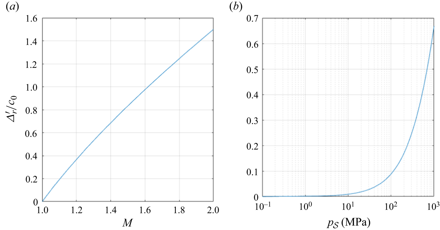
(3.1)\begin{equation} \frac{{\rm d}}{{\rm d} t}(\varDelta_r) = \varDelta_r' = \zeta_{r,F}-\zeta_{r,T} = \frac{1}{2}(\gamma_i+1)(u_R - u_L). \end{equation}

In the case of a rarefaction connecting a quiescent fluid to a shocked fluid (as in the case of a square shock), we have, using the Rankine–Hugoniot relations,

(3.2)\begin{equation} \varDelta_r' = c_0\left(\frac{M^2-1}{M}\right). \end{equation}

Clearly, $\varDelta _r' \rightarrow 0$ as $M\rightarrow 1$, so the rarefaction will remain infinitely thin in this limit. Figure 4 shows how this changes as we move away from the limit. As the Mach number increases, the rate of spread of the wave increases, but because of the stiff nature of water, the shock pressure can rise quite high before this becomes significant. This is why the method set out in this work can readily be applied only to fast–slow problems and not slow–fast problems.

Figure 4.

Time rate of change of width of a rarefaction wave moving into a region of shocked water.

This analysis is used to make the following assumptions in the solution process outlined in figure 3. First, the right-going rarefaction wave at the tail of the square wave remains infinitely thin over $t_1 < t \leq t_2$. Second, the rarefaction created at time $t=t_1$ is infinitely thin over $t_1< t \leq t_2$, and finally, the right-going rarefaction created at $t_2$ remains infinitely thin over $t_2< t\leq t_3$. These assumptions are required only when a rarefaction comes into contact with another wave or discontinuity. Thus for the left-going rarefaction created at $t=t_2$ and the right-going rarefaction created at $t_3$, we do not make this assumption, and the wave structures are computed as per § 2.2. It is noted that Grove & Menikoff (Reference Grove and Menikoff1990) describe the rarefaction wave in the case of the fast–slow interaction of a shock wave in water with a gas bubble as a ‘rarefaction shock’ on account of how thin it is, so these assumptions do have some physical basis. The validity of these assumptions is tested later in this work by comparing with high-order-accurate numerical simulations.

We can now derive the times and locations at which each Riemann problem will take place, which subsequently allows for the widths of the transmitted and reflected pulses to be obtained. The time and location of the second Riemann problem can be computed exactly based on the wave speeds derived from the solution to the first Riemann problem. Note that the assumption during this time period is that the rarefaction does not spread out. The time $t=t_2$ is

(3.3)\begin{equation} t_2 = \frac{-x_T}{2c_\mathcal{S}}, \end{equation}

and the location is

(3.4)\begin{equation} x_2 = \frac{(c_\mathcal{S} - u_\mathcal{S})x_T}{2c_\mathcal{S}}. \end{equation}

The third Riemann problem takes place when the right-going rarefaction reaches the interface:

(3.5)\begin{equation} t_3 = x_T\biggl(\frac{u_s - c_\mathcal{S} - u_1^* - c_{L,1}^*}{2c_\mathcal{S} c_{L,1}^*}\biggr). \end{equation}

The location $x_3$ is then the position of the interface at this time:

(3.6)\begin{equation} x_3 = x_{lg}(t_3)= u_1^*t_3. \end{equation}

This time marks the end of the interaction, leading to a transmitted pulse and a reflected pulse. The width of the reflected pulse at $t=t_3$ is the distance between the contact and the left-going rarefaction wave created at time $t=t_2$. Therefore,

(3.7)\begin{align} \varDelta_{\mathcal{R}} & = x_3 - (x_2+(u_{l,0}-c_{l,0})(t_3-t_2)) \nonumber\\ & ={-}x_T\biggl(\frac{(u_1^* + c_{L,1}^* - u_{l,0} + c_{l,0})(u_1^* + c_\mathcal{S} - u_\mathcal{S})}{2c_{L,1}^*c_\mathcal{S}}\biggr)\geq \varDelta_\mathcal{S}. \end{align}

The width of the reflected pulse is therefore at least the width of the incident shock, with the width increasing as the shock pressure increases due to the higher speed of the interface following the first Riemann problem. The shocked gas is bounded by the portion of the incident shock that was transmitted into the gas at $t=t_1$ and the rarefaction wave created at $t=t_3$. For times $t>t_1$, the position of the right-going shock wave is $x_{\mathcal {S},g}(t) = \zeta _{\mathcal {S},g}t$. Therefore, the width of the shocked region in the gas phase at time $t=t_3$ is

(3.8)\begin{equation} \varDelta_{\mathcal{T}} = \zeta_{\mathcal{S},g}t_3 - x_3 = x_T \biggl(\frac{(u_1^* + c_{L,1}^* - u_\mathcal{S} + c_\mathcal{S}) (u_1^*-\zeta_{\mathcal{S},g})}{2c_{L,1}^*c_\mathcal{S}}\biggr). \end{equation}

3.2. PN-type pulse

The solution strategy for this problem is similar to that of the P-type pulse, with Riemann problems being solved each time two waves interact or a wave interacts with the interface. The solution structure is shown in figure 5 and consists of six Riemann problems. The same assumptions are made that rarefaction waves remain infinitely thin during the intermediate stages. This applies only to waves that will subsequently interact with another wave.

1. (i) $t=t_1$. The right-going shock reaches the liquid–gas interface. This is the first Riemann problem, with the left state being $\boldsymbol {w}_{\mathcal {S},+ve}$, and the right state $\boldsymbol {w}_{g,0}$. As with the positive square wave, the solution consists of a left-going rarefaction and a right-going shock. The interface will move with the velocity determined from this Riemann problem.

2. (ii) $t=t_2$. The left-going rarefaction created at $t=t_1$ reaches the right-going rarefaction that separates the positive and negative parts of the incident pulse. The solution is two rarefaction waves with a constant pressure between them.

3. (iii) $t=t_3$. The left-going rarefaction created at $t_2$ reaches the shock wave at the tail of the pulse. The solution is a left-going rarefaction and a right-going shock. Strictly speaking, this leads to two states, but as will be shown, the density across the discontinuity is extremely small, so the discontinuity may be considered degenerate.

4. (iv) $t=t_4$. The right-going rarefaction created at $t_2$ reaches the interface. If the widths of the two parts of the pulse are similar, then this will likely take place after $t_3$, but this order does not affect the solution. The solution is a left-going shock and a right-going rarefaction. The velocity in the star region is now negative, so the interface will move leftwards.

5. (v) $t=t_5$. The right-going shock created at $t_3$ and the left-going shock created at $t_4$ meet, creating the fifth Riemann problem. The solution is two new shocks propagating in opposite directions: one going left, and one going right, towards the interface.

6. (vi) $t=t_6$. The right-going shock created at $t_5$ reaches the interface, which has been travelling at $u_{L,4}^*$ for $t>t_4$. The solution to this Riemann problem is a left-going rarefaction and a right-going shock.

Figure 5.

Illustration of the stages of the solution for the reflection/transmission of a PN-type pulse. The Riemann problems occurring at $t=t_1,\ldots,t_6$ are shown on the right-hand side, with their left and right initial states. Regions of shocked and rarefied fluid are shown in red and blue, respectively. Shock and rarefaction waves are denoted $s$ and $r$, respectively.

As with the P-type pulse, it can be shown that this solution structure is always the same for a water–air interface, but only for certain pressures. In Appendix B, this is shown for pulses where the magnitude of the pressure in both the negative and positive parts of the pulse is up to 500 MPa. Beyond this, it will be shown in § 4.5 that a vacuum state can be created to the right of the interface, and the present model cannot accommodate such a case. However, this depends on the fluids considered and the value of $p_\infty$. Clearly, a higher value of $p_\infty$ will accommodate lower pressures in the liquid, but this may lead to the gas phase being put into vacuum earlier. Depending on the widths of the two parts of the pulse, $t_4$ may occur before or after $t_3$. For example, if the positive part is very thin compared to the negative part, then it is likely that $t_4$ will occur first. However, Appendix B shows that this will not alter the overall solution. The times and locations of each Riemann problem can again be derived by considering the speeds at which the different waves and the interface travel during the process. These are also given in Appendix B, and can be used to derive the widths of the reflected and transmitted pulses. The reflected pulse is bounded by the rarefaction wave created at time $t=t_3$ and the rarefaction wave created at $t=t_6$. This leads to the expression

(3.9)\begin{equation} \varDelta_\mathcal{R} = x_6 - x_3 - (t_6 - t_3)(u_{l,0}-c_{l,0}). \end{equation}

The transmitted pulse is bound by the shock front that is transmitted into the gas at $t=t_1$ and the shock created at $t_6$. Therefore,

(3.10)\begin{equation} \varDelta_\mathcal{T} = \zeta_{R,1}t_6 - x_6. \end{equation}

The widths of the parts are discussed in subsequent sections in the context of the different regimes: the acoustic limit, weak shocks and strong shocks.

4.1. Comparison with numerical simulations

Thus far, a description of the process of reflection and transmission of two idealised pulses at a liquid–gas interface has been presented. In this subsection, the analytical model is compared to numerical simulations to confirm that it is indeed able to describe the reflection and transmission process. To this end, we employ a well-established front-tracking framework, FronTier (Glimm et al. Reference Glimm, Isaacson, Marchesin and McBryan1981, Reference Glimm, Grove, Li, Shyue, Zeng and Zhang1998; Chern et al. Reference Chern, Glimm, McBryan, Plohr and Yaniv1986; Du et al. Reference Du, Fix, Glimm, Jia, Li, Li and Wu2006; Bempedelis & Ventikos Reference Bempedelis and Ventikos2020b), that solves the compressible Euler equations closed with the SG EoS (see § 2.1). The equations are solved on a uniform grid using a fifth-order WENO scheme and a third-order Runge–Kutta method. In the numerical results presented, a grid convergence study (see Appendix C) has confirmed that numerical diffusion effects are negligible. The employed front-tracking solver has been validated against several experimental and numerical data, as well as benchmark tests, in a wide range of multiphase flow problems involving shock waves and interfaces (Bempedelis & Ventikos Reference Bempedelis and Ventikos2020a,Reference Bempedelis and Ventikosb, Reference Bempedelis and Ventikos2022; Bempedelis et al. Reference Bempedelis, Zhou, Andersson and Ventikos2021).

Suppose that we have a water–air interface initially at $x=0\,\text {m}$. The primitive variables in the ambient liquid and gas are

(4.1a,b)\begin{equation} \boldsymbol{w}_{l,0} = \begin{pmatrix} \rho_{l,0} \\ u_{l,0} \\ p_{l,0} \end{pmatrix} = \begin{pmatrix} 998 \\ 0.0 \\ 1\times10^5 \end{pmatrix},\quad \boldsymbol{w}_{g,0} = \begin{pmatrix} \rho_{g,0} \\ u_{g,0} \\ p_{g,0} \end{pmatrix} = \begin{pmatrix} 1.16 \\ 0.0 \\ 1\times10^5 \end{pmatrix}. \end{equation}

At time $t=t_1$, a right-going square pulse with width $\varDelta _\mathcal {S}=2\times 10^{-4}\,\text {m}$ comes into contact with the interface. For both pulse types considered, the pressure in the positive part is $p_\mathcal {S} = p_{\mathcal {S},+ve} = 10^7$ Pa. For the PN-type pulse, $p_{\mathcal {S},-ve}-p_{l,0} = -(p_{\mathcal {S},+ve} - p_{l,0})$ and $\varDelta _{\mathcal {S},+ve}=\varDelta _{\mathcal {S},-ve}=1\times 10^{-4}\,\text {m}$. The velocity and density in the pulses are determined using the Rankine–Hugoniot relations. Figures 6 and 7 show the solutions for both cases. The initial conditions are shown along with intermediate states, and at time $t=2\times 10^{-7}\,\text {s}$, which is shortly after the process completes in both cases. For the P-type pulse, all intermediate conditions are shown, and the states are labelled to show that the solution does indeed follow the process set out in § 3. For the PN-type pulse, a single intermediate condition is shown for brevity. The agreement between the analytical and numerical predictions is excellent at all stages, showing that the pulse–interface interaction process can indeed be approximated via a small number of wave interactions.

Figure 6.

Analytical and numerical predictions for the reflection/transmission of a P-type pulse ($p_\mathcal {S} = 10\,\text {MPa}$) at a water–air interface: (a) initial conditions; (b) $t=5\times 10^{-8}\,\text {s}$ ($t_1< t< t_2$); (c) $t=1\times 10^{-7}\,\text {s}$ ($t_2< t< t_3$); (d) $t=2\times 10^{-7}\,\text {s}$ ($t_3< t$).

Figure 7.

Analytical and numerical predictions for the reflection/transmission of a PN-type pulse ($\kern0.7pt p_{\mathcal {S},+ve} = 10\,\text {MPa}$) at a water–air interface: (a) initial conditions; (b) $t=8\times 10^{-8}\,\text {s}$ ($t_4 < t < t_5$); (c) $t=2\times 10^{-7}\,\text {s}$ ($t_6< t$).

For the P-type pulse, the reflected pulse puts the liquid into tension. It can also be seen that this happens only when the rarefaction wave meets the tail of the incident pulse, corresponding to the second Riemann problem. Both the numerical and analytical models predict a slightly lower pressure magnitude in the reflected pulse than is predicted by linear theory. Linear theory predicts pressure $-9.89$ MPa, whereas the numerical and analytical approaches lead to reflected pressure $-9.71$ MPa. Whilst this difference is relatively small, it will be shown later that the present theory diverges significantly from linear theory for larger shock pressures. This also means that the pressure in the reflected pulse is not simply a sum of the strength of the left-going rarefaction wave created at $t_1$ and the ambient pressure. The reflected pulse is slightly wider than the incident pulse, and the interface has moved slightly rightwards. This pulse is considered to be ‘weak’, with $u_\mathcal {S} \ll c_{l,0}$, and it can be seen from the numerical results that the rarefaction waves do remain extremely thin over the relevant time scales. This suggests that for weak shock waves at least, the assumptions made in order to derive the analytical solution are valid.

For the PN-type pulse, a reflection of the wave can be seen and the magnitude of the negative pressure is the same as for the P-type pulse. The region in tension is slightly wider that the initial shocked region, again giving the same result as for the P-type pulse. The negative part of the incident pulse reflects as a positive part, and the pressure in this region is higher than would be predicted by linear theory, and also higher than the incident shock pressure. Linear theory predicts reflected pressure 9.89 MPa, whereas both the analytical and numerical models predict 10.09 MPa. Furthermore, while the tension region in the reflected pulse is wider than the incident shocked region, the shocked region in the reflected pulse is slightly narrower. Figure 7(b) also shows that a region with pressure significantly below that of the incident pulse exists in the intermediate state. Referring to figure 5, this is $\boldsymbol {w}_2^*$, and it will exist only temporarily ($t_2< t< t_5$). It comes about when the rarefaction wave created at $t_1$ reaches the rarefaction wave that separates the positive and negative parts of the pulse. The pressure in this state will always be more negative than the pressure in either the incident or reflected parts of the pulse, and should be considered carefully in practical applications as this could lead to significantly higher levels of cavitation depending on the duration for which it exists.

These results show that the proposed analytical approach is valid, with the results closely matching those from high-order numerical simulations of the Euler equations. It is also clear that there are differences between these results and the predictions of linear theory. Given that linear theory allows for the derivation of reflection and transmission coefficients, we will now extend these concepts to the nonlinear problems considered in this work.

4.2. Reflection and transmission coefficients

In the context of this work, the simplest definition of a reflection and transmission coefficient is the ratio of the peak pressure in the reflected and transmitted waves relative to the incident shock pressure. For the P-type pulse, these coefficients are defined as

(4.2)$$\begin{gather} C_\mathcal{R} = \frac{p_2^*-p_{l,0}}{p_\mathcal{S}-p_{l,0}}, \end{gather}$$

(4.3)$$\begin{gather}C_\mathcal{T} = \frac{p_1^*-p_{g,0}}{p_\mathcal{S}-p_{l,0}}. \end{gather}$$

There are two comparisons that we can make here: first with linear theory, and second with a solution derived from a single Riemann problem solved at the interface. As discussed in the Introduction, linear theory results in reflection and transmission coefficients that depend only on the differences in impedance between the media across the interface. An alternative approach is to solve a Riemann problem only at the interface to determine the strength of the right-going shock and the left-going rarefaction. This is what would be obtained if the approach of Henderson (Reference Henderson1989) were to be applied directly to a finite-width pulse. In this case, the pressure in the reflected pulse is the sum of the strength of the rarefaction wave and the ambient pressure in the liquid. Figure 8 shows the reflection and transmission coefficients for a range of shock pressures using the three different approaches. Numerical solutions are also included for comparison. The results are presented for the peak over-pressure $p'_\mathcal {S} = p_\mathcal {S} - p_{l,0}$.

Figure 8.

Reflection and transmission coefficients based on peak pressures for a P-type pulse.

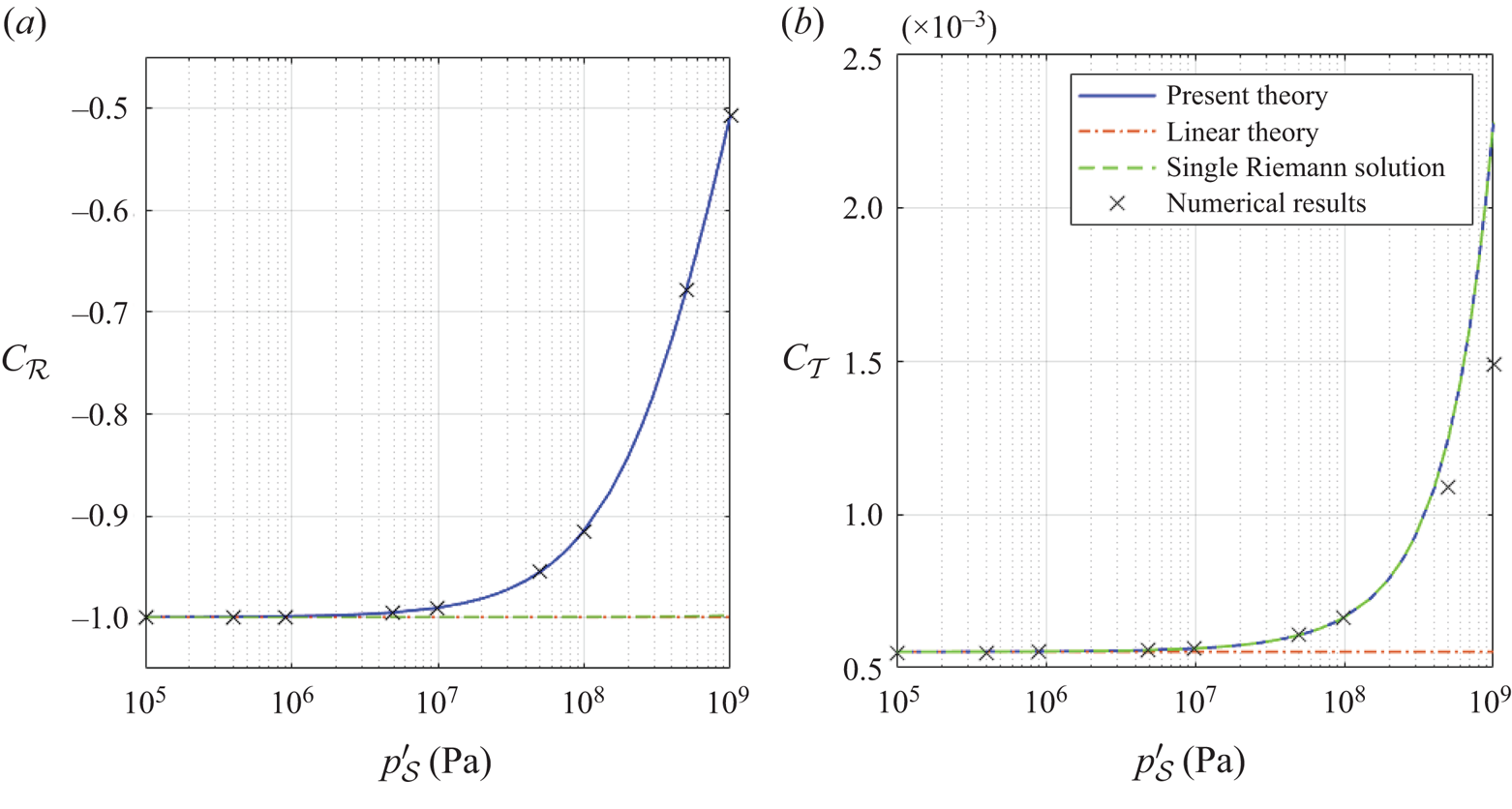
First, it is clear that in the acoustic limit, all methods tend to the same value. Away from this, significant differences are observed. For the reflection coefficient, the current analytical approach and the numerical simulations predict a decrease in the magnitude of the reflection coefficient as the shock pressure increases. This represents a divergence from linear theory as one might expect for what is a highly nonlinear problem. The reflection coefficient derived by solving a single Riemann problem also differs significantly from the present approach, suggesting that the pulse–interface interaction problem cannot be modelled accurately by only considering what happens at the interface. This is because the assumption that wave interactions do not alter the wave properties is not valid. Thus we must consider how the rarefaction wave is altered as it propagates into the region of lower pressure behind the shock. For the transmission coefficient, there are no further interactions, so solving a single Riemann problem at the interface is sufficient. However, it can again be seen that linear theory fails at large shock pressures. The numerical results agree very well with the present analytical approach, although some divergence is seen in the transmission coefficient at higher pressures. This is likely due to the assumptions in solving the interface interaction, i.e. the coupling of the two fluids at the interface, in the numerical methods that we use, that include linearisations, isentropic extrapolations and ‘overheating’ effects (for more details, see Fedkiw, Marquina & Merriman Reference Fedkiw, Marquina and Merriman1999; Hu & Khoo Reference Hu and Khoo2004).

For a pulse with both positive and negative parts, it was shown in the previous section that the two parts reflect differently. It therefore makes sense to consider reflection and transmission coefficients for the two parts separately to understand how and why these vary. The coefficients are defined using specific solutions to the Riemann problems that lead to the reflected and transmitted pulses

(4.4)$$\begin{gather} C_{\mathcal{R}_{{+}ve}} = \frac{p_3^* - p_{l,0}}{p_{\mathcal{S},+ve} - p_{l,0}}, \end{gather}$$

(4.5)$$\begin{gather}C_{\mathcal{R}_{{-}ve}} = \frac{p_5^* - p_{l,0}}{p_{\mathcal{S},-ve} - p_{l,0}}, \end{gather}$$

(4.6)$$\begin{gather}C_{\mathcal{T}_{{+}ve}} = \frac{p_1^* - p_{g,0}}{p_{\mathcal{S},+ve} - p_{l,0}}, \end{gather}$$

(4.7)$$\begin{gather}C_{\mathcal{T}_{{-}ve}} = \frac{p_1^* - p_{g,0}}{p_{\mathcal{S},-ve} - p_{l,0}}. \end{gather}$$

Thus $C_{\mathcal {R},+ve}$ refers to the reflection of the positive part of the incident pulse. We first consider the case where the magnitudes of the over- and under-pressures in the incident pulse are the same. The coefficients are shown in figure 9, along with numerical results. Agreement between the analytical and numerical results is again very good. The reflection of the positive part of the incident wave is the same as for the P-type pulse. The magnitude of the reflection of the negative part increases with shock pressure, meaning that the maximum pressure of the reflected pulse will be greater than the maximum pressure in the incident pulse. This behaviour is mirrored in the transmission coefficients, and again the transmission of the positive part of the pulse is the same as for the positive square wave.

Figure 9.

Reflection and transmission coefficients based on peak pressures for a PN-type pulse where the widths of the two incident regions are constant and $p'_{\mathcal {S},-ve} = -p'_{\mathcal {S},+ve}$. Numerical results are shown with crosses.

Coefficients (4.4)–(4.7) assume that the reflection and transmission of each part of the pulse depend only on the magnitude of that particular part. In many practical applications, the magnitude of the negative part is different from that of the positive part. It is therefore worth considering how these coefficients change when the peak pressure in the negative part is different from that in the positive part. This is shown in figure 10. This tells us two things. First, the reflection of the positive part is independent of the magnitude of the negative part. This has already partly been shown because the reflection coefficient for a P-type wave was the same as that derived for the positive part of the PN-type wave. However, the reflection coefficient of the negative part is dependent on the strength of both the positive and negative parts of the incident pulse.

Figure 10.

Reflection coefficients for a PN-type pulse where the negative and positive pressure magnitudes differ.

For the PN-type pulse, a region of strongly rarefied liquid ($\boldsymbol {w}_2^*$) results when the left-going rarefaction wave created at $t=t_1$ reaches the tail of the positive part of the incident pulse ($t=t_2$). This state exists only for $t_2< t< t_5$. As with the negative part of the reflected pulse, the magnitude of this negative pressure is also a decreasing function in the incident shock pressure. By non-dimensionalising by the difference between the positive and negative pressures in the incident wave so that

(4.8)\begin{equation} C_{\mathcal{R},{tmp}}=\frac{p_2^* - p_{l,0}}{p_{S,+ve} - p_{S,-ve}}, \end{equation}

the pressures in this temporary region all collapse onto a single line for weaker shocks, as shown in figure 11. For shocks where $p_{\mathcal {S},+ve}>100$ MPa, small deviations are seen, with the magnitude of the coefficient reducing for pulses where the relative magnitude of the negative pressure is greater. This pressure will exist only for a time determined by the width of the negative part of the incident pulse. Depending on the width and the minimum pressure that exists during this time, this may be of considerable importance as it could lead to higher levels of cavitation than would be predicted by only considering the final pressures in the reflected pulse.

Figure 11.

Coefficient for the minimum pressure that will exist during the reflection process, as defined by $C_{\mathcal {R},{tmp}}$.

The solution (§ 3) and reflection/transmission coefficients have been derived for an arbitrary set of liquid–gas media modelled with the SG EoS, but their exact values depend on the EoS parameters. In this work, we consider the values $\gamma =2.955$ and $p_\infty =722\,\text {MPa}$ for liquid water, but different values are used in other works, depending on factors such as the temperature. For example, Haller et al. (Reference Haller, Ventikos and Poulikakos2003) use $\gamma =3$, $p_\infty =618$ MPa, and Métayer, Massoni & Saurel (Reference Le Métayer, Massoni and Saurel2004) use $\gamma =2.35$, $p_\infty =1000$ MPa. Irrespective of the particular liquid under consideration, the values of $p_\infty$ do have an effect on the reflection and transmission of the pulse. This is exemplified in figure 12 for a P-type pulse, suggesting two things. First, the level of ‘stiffness’ of the water influences the results significantly only for higher pressures, which is expected as compressibility plays a greater role here. Second, the ‘stiffer’ the water is assumed to be, the smaller the change in the reflection coefficient as the shock pressure increases. The change in the transmission coefficients can be explained more readily using either linear theory or an approximate Riemann solver (e.g. Hu & Khoo Reference Hu and Khoo2004) because the change in $p_\infty$ alters the speed of sound, which in turn changes the impedance.

Figure 12.

(a) Reflection and (b) transmission coefficients for a P-type pulse at a water–air interface with varying values of $p_\infty$, for $\gamma _l=2.955$ and $\gamma _g=1.4$.

As well as considering the pressure in the reflected and transmitted pulses, it is also of interest to consider the velocity. This is shown in figure 13 for both pulse types following the solution to each Riemann problem. For the PN-type pulse, $p'_{\mathcal {S},-ve} = p'_{\mathcal {S},+ve}$ in this example. The particle velocities are remarkably constant as a function of the particle velocity in the incident pulse. Following the initial interaction of the shock front with the interface, the interface will move rightwards at $u^*_1 \approx 2u_\mathcal {S}$ for all shock pressures. It is interesting to note that this is the same as the particle velocity obtained for a linear problem by considering the limit as the difference in impedance becomes very large. This relationship was also noted by Grove & Menikoff (Reference Grove and Menikoff1990) when considering a similar fast–slow problem for a shock wave. For the P-type pulse, $u_1^*$ is the velocity in the transmitted pulse, and $u_2^*$ is the velocity in the reflected pulse. Also, $u_3^*$ is the velocity of the fluid in between the reflected and transmitted pulses, and it can be seen that this is zero for all shock pressures, again demonstrating that the entire process results in only a reflected and transmitted pulse with no further changes to either fluid. For the PN-type pulse, as with the P-type pulse, the interface will initially move at $u_1^* \approx 2u_\mathcal {S}$, this time over the interval $t_1 < t < t_4$. The solution to the fourth Riemann problem then reverses the interface, with the magnitude being almost exactly the same for all but the largest shocks. Finally, the interface is stopped at $t_6$, signifying the end of the process.

Figure 13.

Particle velocity in the star regions following each Riemann problem: (a) P-type pulse; (b) PN-type pulse.

4.3. The acoustic limit

To provide further insights into the properties of the reflected and transmitted waves, it is useful to consider the problem in three different regimes: the acoustic limit, the weak shock regime and the strong shock regime. Formally, the acoustic limit is defined by $M\rightarrow 1^+$. The particle velocities tend to zero, and the wave speeds all tend to the sound speed in the relevant fluid. It has already been shown that any rarefaction waves will remain infinitely thin in the acoustic limit. Since this is the only assumption made in the derivation in § 3, the method is exact in this limit.

The reflection and transmission coefficients were all shown to tend to the values predicted by linear theory in figures 8, 9 and 10. Furthermore, we also have that

(4.9)\begin{equation} \lim_{M\rightarrow 1^+} u_\mathcal{S} = 0, \end{equation}

so $u_i^* \rightarrow 0$ for both pulses. The sound speeds and wave speeds will all tend to the ambient speeds in the respective fluids. For a P-type pulse, the width of the reflected wave, $\varDelta _{\mathcal {R}}$, is obtained by taking the limit of (3.7):

(4.10)\begin{equation} \lim_{M\to 1^+} \varDelta_\mathcal{R} ={-}x_T = \varDelta_\mathcal{S} \end{equation}

and

(4.11)\begin{equation} \lim_{M\to 1^+} t_3 ={-}x_T/c_{l,0}. \end{equation}

In other words, the width of the reflected pulse is exactly the same as the width of the incident pulse. The width of the transmitted pulse can be found by taking the limit of (3.8):

(4.12)\begin{equation} \lim_{M\to 1^+} \varDelta_\mathcal{T} ={-}x_T\,\frac{c_{g,0}}{c_{l,0}}. \end{equation}

That is, the width of the transmitted pulse is equal to the width of the incident pulse multiplied by the ratio of the sound speeds of the two fluids. This is analogous to the linear case, where the wavelength reduces proportional to the ratio of sound speeds of the two fluids.

Using the same argument for a PN-type pulse,

(4.13)\begin{equation} \lim_{M\to 1^+} x_6 = 0, \end{equation}

so the interface will also remain in the same place in the acoustic limit. The reflected and transmitted pulse widths are found by taking the limit of (3.9) and (3.10) as $M\rightarrow 1^+$, and it is straightforward to show that these lead to the same expressions as for the P-type pulse.

4.4. Weak shocks

Moving away from the acoustic limit, the assumptions that the particle velocities are zero and the Mach number is $M = 1$ are no longer valid. This represents a departure from where linear theory is formally valid. For a weak shock, it is assumed that $u_\mathcal {S}$ remains small compared to $c_{l,0}$. Therefore, the rarefaction waves will remain very thin over the relevant time scales. For the P-type pulse, the negative pressure in the reflected pulse comes about following the second Riemann problem. For weak shocks, the pressure behind the rarefaction wave produced by the initial interaction of the shock and the interface remains roughly constant at levels slightly above the ambient pressure. Therefore, the solution to the second Riemann problem is determined primarily by the difference in the particle velocities. The increasing positive velocity in the right initial state as the incident shock pressure increases leads to a rarefied region with an increasingly negative pressure.

For weak shocks, because the solution to the first Riemann problem yields a pressure that is very close to the ambient pressure, it is possible to derive a closed-form approximate expression for the reflected and transmitted wave using the solution derived in § 3. The interface moves with $u_1^* \approx 2u_S$ for $t_1 \leq t \leq t_3$, corresponding to the liquid becoming rarefied and the gas becoming compressed. For a weak incident shock, $p_1^*$ is only slightly larger than $p_{l,0}$, so $c_{L,1}^* \approx c_{l,0}$. Therefore, using these two approximations, we can rewrite $x_3$ as

(4.14)\begin{equation} x_3 \approx{-}u_\mathcal{S} x_T \left(\frac{c_{l,0} + c_\mathcal{S} + u_\mathcal{S}}{c_\mathcal{S} c_{l,0}}\right). \end{equation}

Using the same assumptions and assuming that the ambient liquid is at rest, the width of the rarefied region at $t=t_3$ is

(4.15)\begin{equation} \varDelta_\mathcal{R} \approx{-}x_T \left(\frac{(c_{l,0}+u_\mathcal{S}) (c_\mathcal{S}+u_\mathcal{S})}{c_{l,0}c_\mathcal{S}}\right). \end{equation}

We now call upon the conservation of mass in the liquid. Comparing the initial state and that at $t=t_3$, we have

(4.16)\begin{equation} \int_{-\infty}^{x_T}\rho_{l,0}\,{{\rm d}\kern0.7pt x} + \int_{x_T}^{0}\rho_\mathcal{S}\,{\rm d}x = \int_{-\infty}^{x_3 - \varDelta_\mathcal{R}} \rho_{l,0}\,{{\rm d}\kern0.7pt x} + \int_{x_3-\varDelta_\mathcal{R}}^{x_3} \rho_2^*\,{{\rm d}\kern0.7pt x}. \end{equation}

Evaluating this and rearranging gives

(4.17)\begin{equation} \rho_2^* = \frac{\rho_{l,0}(x_T + \varDelta_\mathcal{R}-x_3) -\rho_\mathcal{S} x_T}{\varDelta_\mathcal{R}} = \frac{c_{l,0} c_\mathcal{S} \rho_\mathcal{S}}{(c_0+u_\mathcal{S})(c_\mathcal{S}+u_\mathcal{S})}. \end{equation}

The pressure in the rarefied region can be obtained by rearranging the Rankine–Hugoniot relations (2.5) and (2.6):

(4.18)\begin{equation} p_2^* = \frac{(p_{l,0}+p_\infty)(1+\gamma_l)}{1+\gamma_l \left(\dfrac{4\rho_{l,0}}{\rho_{l,0}(1-\gamma_l)+\rho_2^*(1+\gamma_l)}-1\right)} - p_\infty. \end{equation}

Similarly, in the gas we have that

(4.19)\begin{equation} \int_0^\infty \rho_{g,0}\,{{\rm d}\kern0.7pt x} = \int_{x_3}^{x_3+\varDelta_\mathcal{T}} \rho_{R,1}^*\,{{\rm d}\kern0.7pt x} + \int_{x_3+\varDelta_\mathcal{T}}^\infty p_{g,0}\,{{\rm d}\kern0.7pt x}. \end{equation}

The shock wave that propagates into the gas is very weak in comparison to that in the liquid, so $\zeta _{\mathcal {S},g} \approx c_{g,0}$. Using this, we can obtain the following expression for $\rho _{R,1}^*$, which again depends only on the initial data:

(4.20)\begin{equation} \rho_{R,1}^* = \frac{c_{g,0}\rho_{g,0}}{c_{g,0}-2u_\mathcal{S}}. \end{equation}

The pressure in the shocked gas can again be obtained by way of the Rankine–Hugoniot relations. These expressions enable the reflection–transmission of a shock wave at a liquid–gas interface to be computed without solving a Riemann problem, potentially allowing for the approach to be more easily integrated into other applications.

This also has a useful physical interpretation, explaining how a region of rarefied liquid (where $p< p_{l,0}$ and $\rho <\rho _{l,0}$) can result from a region of shocked liquid. For a solution consisting of only a left-going rarefied region (in the liquid), the only way for mass in the liquid to be conserved is for the interface to move rightwards to precisely compensate for the difference in the mass of the incident and reflected pulses. Should this not happen (e.g. if the interface velocity was altered by some other mechanism), then additional waves would be created in order to balance out the mass in the liquid. However, in the case of a weak shock, these differences are balanced by the movement of the interface. For the PN-type pulse, the interface initially moves rightwards before moving leftwards for $t_4 < t < t_6$. This explains why the negative part of the reflected pulse is wider, and the positive part is narrower. Noting these changes in the widths of the pulse, it is also useful to consider the total ‘strength’ of the reflected and transmitted pulses by integrating the pressure over their respective widths. For the P-type pulse, modified reflection and transmission coefficients can therefore be defined as

(4.21)$$\begin{gather} \hat{C}_\mathcal{R} = \frac{\displaystyle\int_{\varDelta_\mathcal{R}}(p - p_{l,0})\,{{\rm d}\kern0.7pt x}}{ \displaystyle\int_{\varDelta_\mathcal{S}}(p_\mathcal{S}-p_{l,0})\,{{\rm d}\kern0.7pt x}} , \end{gather}$$

(4.22)$$\begin{gather}\hat{C}_\mathcal{T} = \frac{\displaystyle\int_{\varDelta_\mathcal{T}}(p - p_{g,0})\,{{\rm d}\kern0.7pt x}}{ \displaystyle\int_{\varDelta_\mathcal{S}}(p_\mathcal{S}-p_{l,0})\,{{\rm d}\kern0.7pt x}} . \end{gather}$$

For the PN-type pulse, we again consider the reflection of the positive and negative parts separately:

(4.23)$$\begin{gather} \hat{C}_{\mathcal{R},+ve} = \frac{\displaystyle\int_{\varDelta_{\mathcal{R},-ve}}(p - p_{l,0})\, {{\rm d}\kern0.7pt x}}{\displaystyle\int_{\varDelta_{\mathcal{S},+ve}}(p_{\mathcal{S},+ve}-p_{l,0})\,{{\rm d}\kern0.7pt x}}, \end{gather}$$

(4.24)$$\begin{gather}\hat{C}_{\mathcal{R},-ve} = \frac{\displaystyle\int_{\varDelta_{\mathcal{R},+ve}}(p - p_{l,0})\,{{\rm d}\kern0.7pt x}}{\displaystyle\int_{\varDelta_{\mathcal{S},-ve}}(p_{\mathcal{S},-ve}-p_{l,0})\,{{\rm d}\kern0.7pt x}}. \end{gather}$$

Similar expressions can be written for the modified transmission coefficients. For the P-type pulse, the modified reflection coefficient is less sensitive to the incident shock pressure than the coefficient presented earlier. This is shown in figure 14(a) and is because the drop in the pressure magnitude in the reflected pulse is partially offset by the increase in its width. A similar pattern is observed for the PN-type pulse. The wider reflected pulse offsets the reduction in the pressure magnitude, although by less than for the P-type pulse. In the weak regime where the rarefaction waves are assumed to not spread out, the modified reflection and transmission coefficients for the P-type pulse are independent of the incident pulse width. For the PN-type pulse, this is true only when $\varDelta _{\mathcal {S},+ve}/\varDelta _{\mathcal {S},-ve}$ is constant. If the relative widths vary, then differences are seen in the modified coefficients even for weak shocks, as shown in figure 14(b). This shows the two modified reflection coefficients for a range of width ratios. For a water–air interface, the magnitude of $\hat {C}_{\mathcal {R},+ve}$ is always less than would be predicted by linear theory. Whilst this coefficient is less dependent on the negative part of the pulse than the negative coefficient is on the positive part, there is still a weak dependency, because the rarefaction wave at the front of the reflected pulse has interacted with the negative portion of the incident wave. The reflection coefficient of the negative portion of the pulse is more sensitive to changes in the pulse parameters, which is to be expected because it depends more strongly on the positive portion as well as the negative portion. This again highlights the nonlinearity of the process even for weak shocks.

Figure 14.

Modified reflection coefficients for: (a) both P-type and PN-type pulses (for the PN-type pulse, the widths and magnitudes of over- and under-pressures are equal); (b) the PN-type pulse with varying width and pressure ratios, where $p'_{\mathcal {S},+ve}=10$ MPa.

4.5. Strong shocks

As we move away from the weak shock regime, the assumption made in this study regarding rarefaction waves starts to break down. Figure 15 shows the pressure, velocity and density at time $t=2\times 10^{-7}\,\text {s}$ for a P-type pulse with $p_\mathcal {S}=5\times 10^8\,\text {Pa}$. The agreement between the analytical approach and the numerical simulations for the minimum/maximum pressure in the reflected/transmitted pulse is again very good, but there are discrepancies with the overall shape. This is because the assumption that the rarefaction waves remain infinitely thin over the relevant time scales becomes increasingly less valid as the shock pressure increases. The particle velocity in the shock and reflected waves is $284\,\text {m}\,\text {s}^{-1}$, and this leads to the rarefaction waves spreading out, even over short time scales. The analytical solution allows for the leftmost rarefaction wave to spread out for $t> t_2$, so it is not infinitely thin; but because it is not allowed to spread out for $t_1\leq t \leq t_2$, it appears thinner than is predicted by the simulation. The same effect is seen in the left-going shock that propagates into the rarefied liquid. In the analytical approach, this is a single shock resulting from the infinitely thin rarefaction arriving at the contact at $t=t_3$. In the numerical simulation, this wave has spread out slightly, effectively leading to the formation of a series of shocks that look like an inverse rarefaction wave. It should be noted that this problem could be ameliorated by splitting up the rarefaction waves into segments and then treating each segment as an individual wave. This would increase the number of wave interactions taking place, and hence the number of Riemann problems to be solved. Such an approach is permissible in this framework, but is beyond the scope of what we consider here.

Figure 15.

Pressure, density, and velocity at $t=2\times 10^7\,\text {s}$ following interaction of a P-type pulse with $p_\mathcal {S}=5 \times 10^8\,\text {Pa}$ with a water–air interface.

Because the magnitude of the reflection coefficient reduces with increasing shock pressure (see figure 8), positive shock pressures greater than $p_\infty$ are permissible. From a mathematical standpoint, a solution can be obtained provided that the pressure does not drop below $-p_\infty$. When using the approach set out in this study, we suggest $p_\infty$ as an appropriate limit for the maximum shock pressure.

For the PN-type pulse, another limiting factor must be considered. At time $t=t_4$, the negative part of the incident pulse starts to transmit into the gas phase. The solution to the Riemann problem at this time determines the pressure and density behind the rarefaction wave that propagates into the gas phase. A pressure or density of zero would imply a vacuum, and this presents a limit to the model presented in this work. Figure 16 shows the pressure in the negative portion of the transmitted wave following the solution to the fourth Riemann problem as a function of the pressure in the negative portion of the incident pulse. As can be seen, for a water–gas interface at atmospheric pressure, the gas will be put into a vacuum state once the negative pressure in the incident shock drops below approximately $-$500 MPa. However, it can also be seen that this is dependent on the pressure in the positive part of the incident pulse as well as the negative part. Higher positive shock pressures require lower negative pressures to put the gas into vacuum. For $p'_{\mathcal {S},-ve}/p'_{\mathcal {S},+ve}=-0.5$, the model predicts that the pressure in the liquid will drop below $p_\infty$ before the pressure in the gas reaches zero. This further highlights the nonlinear behaviour that arises from the different wave interactions, particularly as the pressure magnitudes increase.

Figure 16.

Pressure in the negative portion of the transmitted pulse in the gas phase.

It is important to note that the reflection of many of these stronger shocks would likely induce cavitation, which would radically alter the dynamics of the fluid, and it is beyond the scope of this work to consider this problem.