


1 Introduction
There has been much work in recent years on Stern’s diatomic sequence (e.g. [Reference Calkin and WilfCW00]), fence posets (e.g. [Reference Oğuz and RavichandranOR23]), and q-deformed rational numbers (e.g. [Reference Morier-Genoud and OvsienkoMGO20]), with links between these topics. We strengthen these links by bringing into the foreground hyperbinary partitions. These are partitions in which all parts are powers of two and in which no part appears more than twice. These have appeared in the literature on Stern’s diatomic sequence, but it has not been noticed that these objects relate to order ideals in fence posets and that a natural statistic on these partitions gives a nice way to construct the q-deformed rational numbers, avoiding explicit reliance on continued fractions. We explain those additional links.
In view of the central role to be played by hyperbinary partitions, we first establish some definitions and notation about integer partitions in general. If
 $\lambda $
is an integer partition then we will write it either as a weakly decreasing sequence of integers
$\lambda $
is an integer partition then we will write it either as a weakly decreasing sequence of integers
 $\lambda =(\lambda _1,\lambda _2,\ldots ,\lambda _\ell )$
or in terms of multiplicities
$\lambda =(\lambda _1,\lambda _2,\ldots ,\lambda _\ell )$
or in terms of multiplicities
 $$ \begin{align*}\lambda=\{\!\{ 1^{m_1}, 2^{m_2}, \ldots, n^{m_n}\}\!\} \end{align*} $$
where
 $$ \begin{align*}m_i = m_i(\lambda) =\text{the number of }i\text{'s in } \lambda. \end{align*} $$
When using multiplicity notation in examples, we will often dispense with the commas and multiset braces. When the multiplicity
 $m_i$
is 1, we write
$m_i$
is 1, we write
 $i^1$
as i; when the multiplicity
$i^1$
as i; when the multiplicity
 $m_i$
is 0, we omit
$m_i$
is 0, we omit
 $i^0$
entirely. For example, the integer partition
$i^0$
entirely. For example, the integer partition
 $(4,1,1)$
can be written as
$(4,1,1)$
can be written as
 $1^2 4$
. We may also choose to list the parts in an order other than increasing, writing
$1^2 4$
. We may also choose to list the parts in an order other than increasing, writing
 $1^2 4$
as
$1^2 4$
as
 $4 1^2$
or even
$4 1^2$
or even
 $141$
. Regardless of the notation chosen, if
$141$
. Regardless of the notation chosen, if
 $\lambda $
is a partition of n (meaning that the sum of its parts is n) then we will write
$\lambda $
is a partition of n (meaning that the sum of its parts is n) then we will write
 $\lambda \vdash n$
. The length of
$\lambda \vdash n$
. The length of
 $\lambda $
is
$\lambda $
is
 $$ \begin{align*}\ell(\lambda) = \text{the number of parts of }\lambda = \sum_{i} m_i (\lambda). \end{align*} $$
Returning to our example,
 $\ell (4,1,1)=3$
.
$\ell (4,1,1)=3$
.
Call a partition
 $\eta $
hyperbinary if
$\eta $
hyperbinary if
-
1. each part is a power of
 $2$
, and
$2$
, and -
2. the multiplicity of each part is at most
$2$
.


It appears that Wilf coined this term. The first in-depth study of such partitions was made by Reznick [Reference ReznickRez90], though antecedents can be found going as far back as Stern [Reference SternSte58]. Let
 $$ \begin{align} H(n) = \{\eta \mid \eta \text{ is a hyperbinary partition of } n\} \end{align} $$
and
 $$ \begin{align*}h(n) = \#H(n) \end{align*} $$
where we will use
 $\#S$
or
$\#S$
or
 $|S|$
for the cardinality of a set S. For example,
$|S|$
for the cardinality of a set S. For example,
 $$ \begin{align*}H(10) = \{82,\ 81^2,\ 4^2 2,\ 4^2 1^2,\ 4 2^2 1^2\} \end{align*} $$
so that
 $$ \begin{align*}h(10) = 5. \end{align*} $$
We introduce the generating function
 $$ \begin{align} h_q(n) = \sum_{\eta\in H(n)} q^{\ell(\eta)}. \end{align} $$
For instance,
 $$ \begin{align*}h_q(10) = q^2 + 2q^3 + q^4 + q^5. \end{align*} $$
Clearly
 $h_1(n) = h(n)$
. We will give three applications using
$h_1(n) = h(n)$
. We will give three applications using
 $h_q(n)$
.
$h_q(n)$
.
Our first application, which is in the next section, involves the Calkin-Wilf sequence
 $\operatorname {\mathrm {CW}}(n)$
,
$\operatorname {\mathrm {CW}}(n)$
,
 $n\ge 0$
. This sequence is defined as the ratio
$n\ge 0$
. This sequence is defined as the ratio
 $\operatorname {\mathrm {CW}}(n)=\operatorname {\mathrm {fusc}}(n)/\operatorname {\mathrm {fusc}}(n+1)$
where
$\operatorname {\mathrm {CW}}(n)=\operatorname {\mathrm {fusc}}(n)/\operatorname {\mathrm {fusc}}(n+1)$
where
 $\operatorname {\mathrm {fusc}}(n)$
is Stern’s diatomic sequence as reinvented by Dijkstra (see (3)). The Calkin-Wilf sequence goes through each nonnegative rational number exactly once. Morier-Genoud and Ovsienko gave a way of associating with any rational number
$\operatorname {\mathrm {fusc}}(n)$
is Stern’s diatomic sequence as reinvented by Dijkstra (see (3)). The Calkin-Wilf sequence goes through each nonnegative rational number exactly once. Morier-Genoud and Ovsienko gave a way of associating with any rational number
 $r/s$
a q-analogue which is a rational function
$r/s$
a q-analogue which is a rational function
 $[r/s]_q$
. Our main result of this section is that one can calculate the q-analogue of
$[r/s]_q$
. Our main result of this section is that one can calculate the q-analogue of
 $\operatorname {\mathrm {CW}}(n)$
using the polynomials
$\operatorname {\mathrm {CW}}(n)$
using the polynomials
 $h_q(n)$
. More precisely, we show in Theorem 2.3 that
$h_q(n)$
. More precisely, we show in Theorem 2.3 that
 $$ \begin{align*}[\operatorname{\mathrm{CW}}(n)]_q = q\, \frac{h_q(n-1)}{h_q(n)}. \end{align*} $$
In Section 3, we consider the poset (partially ordered set)
 ${\cal H}(n)$
of hyperbinary partitions of n under the refinement ordering. A fence is a poset obtained by taking a sequence of chains and alternately identifying their maxima and minima. Our principal result here is the isomorphism in Theorem 3.16 which shows that
${\cal H}(n)$
of hyperbinary partitions of n under the refinement ordering. A fence is a poset obtained by taking a sequence of chains and alternately identifying their maxima and minima. Our principal result here is the isomorphism in Theorem 3.16 which shows that
 ${\cal H}(n)\cong {\cal J}({\cal F}(n))$
where
${\cal H}(n)\cong {\cal J}({\cal F}(n))$
where
 ${\cal F}(n)$
is the fence associated with n, and
${\cal F}(n)$
is the fence associated with n, and
 ${\cal J}(P)$
is the distributive lattice of all lower order ideals of the poset P under inclusion. We note that Aval and Labbé [Reference Aval and LabbéAL25] considered an interpretation of q-deformed rationals using order ideals of fence posets, as well as two other interpretations using Ostrowski’s numeration system for integers and perfect matchings of snake graphs.
${\cal J}(P)$
is the distributive lattice of all lower order ideals of the poset P under inclusion. We note that Aval and Labbé [Reference Aval and LabbéAL25] considered an interpretation of q-deformed rationals using order ideals of fence posets, as well as two other interpretations using Ostrowski’s numeration system for integers and perfect matchings of snake graphs.
Section 4 is devoted to the study of certain q-analogues of the standard generators of
 $\operatorname {\mathrm {SL}}(2,{\mathbb Z})$
, see (28). Morier-Genoud and Ovsienko showed that their rational q-analogues can be computed using certain products of these matrices. We prove in Theorem 4.2 that the entries of such products can be easily computed using the
$\operatorname {\mathrm {SL}}(2,{\mathbb Z})$
, see (28). Morier-Genoud and Ovsienko showed that their rational q-analogues can be computed using certain products of these matrices. We prove in Theorem 4.2 that the entries of such products can be easily computed using the
 $h_q(n)$
.
$h_q(n)$
.
We end with a section devoted to open questions and avenues for future research.
2 A q-analogue of the Calkin-Wilf sequence
Let
 ${\mathbb N}$
and
${\mathbb N}$
and
 ${\mathbb Q}$
be the nonnegative integers and the rationals, respectively. Stern’s diatomic sequence, also known as the Stern-Brocot sequence or the obfuscating sequence, can be defined inductively as
${\mathbb Q}$
be the nonnegative integers and the rationals, respectively. Stern’s diatomic sequence, also known as the Stern-Brocot sequence or the obfuscating sequence, can be defined inductively as
 $\operatorname {\mathrm {fusc}}(0) = 0$
,
$\operatorname {\mathrm {fusc}}(0) = 0$
,
 $\operatorname {\mathrm {fusc}}(1) = 1$
, and for
$\operatorname {\mathrm {fusc}}(1) = 1$
, and for
 $n\ge 1$
,
$n\ge 1$
,
 $$ \begin{align} \begin{array}{rcl} \operatorname{\mathrm{fusc}}(2n) &=& \operatorname{\mathrm{fusc}}(n),\\ \operatorname{\mathrm{fusc}}(2n+1)&=& \operatorname{\mathrm{fusc}}(n+1)+\operatorname{\mathrm{fusc}}(n) \end{array} \end{align} $$
(see Table 1). To our knowledge, Stern [Reference SternSte58] was the first person to study this sequence. The
 $\operatorname {\mathrm {fusc}}$
notation was coined by Dijkstra [Reference DijkstraDij82, pp. 215-216]. For a history of this sequence, see the article of Northshield [Reference NorthshieldNor10].
$\operatorname {\mathrm {fusc}}$
notation was coined by Dijkstra [Reference DijkstraDij82, pp. 215-216]. For a history of this sequence, see the article of Northshield [Reference NorthshieldNor10].
The functions
 $\operatorname {\mathrm {fusc}}_n$
,
$\operatorname {\mathrm {fusc}}_n$
,
 $\operatorname {\mathrm {CW}}_n$
,
$\operatorname {\mathrm {CW}}_n$
,
 $\operatorname {\mathrm {fusc}}_n(q)$
and
$\operatorname {\mathrm {fusc}}_n(q)$
and
 $\operatorname {\mathrm {CW}}_n(q)$

The Calkin-Wilf sequence is defined for all
 $n\ge 0$
by
$n\ge 0$
by
 $$ \begin{align*}\operatorname{\mathrm{CW}}(n) = \frac{\operatorname{\mathrm{fusc}}(n)}{\operatorname{\mathrm{fusc}}(n+1)}. \end{align*} $$
This function has the property that for each rational number
 $r/s \geq 0$
there is a unique integer
$r/s \geq 0$
there is a unique integer
 $n \geq 0$
satisfying
$n \geq 0$
satisfying
 $\operatorname {\mathrm {CW}}(n) = r/s$
. Calkin and Wilf introduced this sequence in [Reference Calkin and WilfCW00] and related the
$\operatorname {\mathrm {CW}}(n) = r/s$
. Calkin and Wilf introduced this sequence in [Reference Calkin and WilfCW00] and related the
 $\operatorname {\mathrm {fusc}}$
function to hyperbinary partitions.
$\operatorname {\mathrm {fusc}}$
function to hyperbinary partitions.
We mention here a method for computing n from
 $r/s$
that is essentially described in [Reference Calkin and WilfCW98] and deserves to be better known. Recall that every positive rational number
$r/s$
that is essentially described in [Reference Calkin and WilfCW98] and deserves to be better known. Recall that every positive rational number
 $r/s$
has two representations as continued fractions, that is, representations of the form
$r/s$
has two representations as continued fractions, that is, representations of the form
 $$ \begin{align} \frac{r}{s}= a_1+\frac{1}{\displaystyle{a_2 + \frac{1}{\ddots + \displaystyle{\frac{1}{a_m}}}}} \end{align} $$
where
 $a_1 \geq 0$
and
$a_1 \geq 0$
and
 $a_2,\dots ,a_m \geq 1$
; for instance,
$a_2,\dots ,a_m \geq 1$
; for instance,
 $7/3$
can be written as both
$7/3$
can be written as both
 $2+1/3$
(with
$2+1/3$
(with
 $m=2$
) and as
$m=2$
) and as
 $2+1/(2+1/1)$
(with
$2+1/(2+1/1)$
(with
 $m=3$
). Given
$m=3$
). Given
 $r/s$
, pick the representation with odd length. Create a binary string consisting of
$r/s$
, pick the representation with odd length. Create a binary string consisting of
 $a_1$
ones, followed by
$a_1$
ones, followed by
 $a_2$
zeros, followed by
$a_2$
zeros, followed by
 $a_3$
ones, followed by
$a_3$
ones, followed by
 $a_4$
zeros, …, followed by
$a_4$
zeros, …, followed by
 $a_m$
ones. Reverse it and one obtains the binary representation of the unique n satisfying
$a_m$
ones. Reverse it and one obtains the binary representation of the unique n satisfying
 $\operatorname {\mathrm {CW}}(n) = r/s$
. For instance, with
$\operatorname {\mathrm {CW}}(n) = r/s$
. For instance, with
 $r/s = 7/3 = 2+1/(2+1/1)$
we form the bit-string 11001 whose reversal
$r/s = 7/3 = 2+1/(2+1/1)$
we form the bit-string 11001 whose reversal
 $10011$
is the binary expansion of the number 19, and one can check that
$10011$
is the binary expansion of the number 19, and one can check that
 $\operatorname {\mathrm {fusc}}(19) = 7$
and
$\operatorname {\mathrm {fusc}}(19) = 7$
and
 $\operatorname {\mathrm {fusc}}(20) = 3$
yielding
$\operatorname {\mathrm {fusc}}(20) = 3$
yielding
 $\operatorname {\mathrm {CW}}(19) = 7/3$
.
$\operatorname {\mathrm {CW}}(19) = 7/3$
.
We will need three operations on partitions. Suppose
 $\lambda =\{\!\{ 1^{m_1}, 2^{m_2}, \ldots , n^{m_n}\}\!\} $
and
$\lambda =\{\!\{ 1^{m_1}, 2^{m_2}, \ldots , n^{m_n}\}\!\} $
and
 $\mu =\{\!\{ 1^{k_1}, 2^{k_2}, \ldots , n^{k_n}\}\!\} $
. Then their sum is the partition
$\mu =\{\!\{ 1^{k_1}, 2^{k_2}, \ldots , n^{k_n}\}\!\} $
. Then their sum is the partition
 $$ \begin{align} \lambda+\mu = \{\!\{ 1^{m_1+k_1}, 2^{m_2+k_2}, \ldots, n^{m_n+k_n}\}\!\}. \end{align} $$
If
 $k_i\le m_i$
for all i then their difference is
$k_i\le m_i$
for all i then their difference is
 $$ \begin{align} \lambda-\mu = \{\!\{ 1^{m_1-k_1}, 2^{m_2-k_2}, \ldots, n^{m_n-k_n}\}\!\}. \end{align} $$
If t is a positive rational number and
 $\lambda =(\lambda _1,\lambda _2,\ldots ,\lambda _\ell )$
then their product is
$\lambda =(\lambda _1,\lambda _2,\ldots ,\lambda _\ell )$
then their product is
 $$ \begin{align} t\lambda = (t\lambda_1,t\lambda_2,\ldots,t\lambda_\ell) \end{align} $$
provided that
 $t\lambda _i\in {\mathbb N}$
for all i. We extend these operations to sets
$t\lambda _i\in {\mathbb N}$
for all i. We extend these operations to sets
 $\Lambda $
of partitions by letting
$\Lambda $
of partitions by letting
 $$ \begin{align} \Lambda+\mu & =\{\lambda+\mu \mid \lambda\in\Lambda\}, \end{align} $$
 $$ \begin{align} \Lambda-\mu & =\{\lambda-\mu \mid \lambda\in\Lambda\}, \end{align} $$
 $$ \begin{align} t\Lambda & =\{t\lambda \mid \lambda\in\Lambda\}, \end{align} $$
provided the sets of the right sides of the equal signs are sets of partitions.
With respect to the three operations, we have
 $$ \begin{align} \ell(\lambda+\mu) &= \ell(\lambda)+\ell(\mu), \end{align} $$
 $$ \begin{align} \ell(\lambda-\mu) &= \ell(\lambda)-\ell(\mu), \end{align} $$
 $$ \begin{align} \ell(t\lambda) &=\ell(\lambda). \end{align} $$
We now show that the sets
 $H(n)$
defined by (1) have a nice recursive structure. Let
$H(n)$
defined by (1) have a nice recursive structure. Let
 $\epsilon $
denote the empty partition and
$\epsilon $
denote the empty partition and
 $\uplus $
denote the disjoint-union operation on sets. The following result is in [Reference Calkin and WilfCW00], but we include its proof for completeness.
$\uplus $
denote the disjoint-union operation on sets. The following result is in [Reference Calkin and WilfCW00], but we include its proof for completeness.
Proposition 2.1 [Reference Calkin and WilfCW00].
We have
 $H(-1)=\emptyset $
,
$H(-1)=\emptyset $
,
 $H(0) = \{ \epsilon \}$
, and for
$H(0) = \{ \epsilon \}$
, and for
 $n\ge 1$
 $$ \begin{align} H(2n-1) &= 2H(n-1)+(1), \end{align} $$
 $$ \begin{align} H(2n) &= 2H(n) \uplus [2H(n-1) +(1^2)]. \end{align} $$
Proof. For equation (14), note that if
 $\eta \in H(2n-1)$
then
$\eta \in H(2n-1)$
then
 $m_1(\eta )=1$
since
$m_1(\eta )=1$
since
 $\eta $
is a hyperbinary partition of an odd number. Thus
$\eta $
is a hyperbinary partition of an odd number. Thus
 $\eta -(1)$
is a hyperbinary partition of
$\eta -(1)$
is a hyperbinary partition of
 $2n-2$
with all parts at least
$2n-2$
with all parts at least
 $2$
. It follows that
$2$
. It follows that
 $\eta -(1)=2\psi $
for some
$\eta -(1)=2\psi $
for some
 $\psi \in H(n-1)$
and the desired equality follows.
$\psi \in H(n-1)$
and the desired equality follows.
Now consider (15). If
 $\eta \in H(2n)$
then
$\eta \in H(2n)$
then
 $1$
appears with multiplicity zero or two. In the first case
$1$
appears with multiplicity zero or two. In the first case
 $\eta =2\psi $
where
$\eta =2\psi $
where
 $\psi \in H(n)$
. In the second,
$\psi \in H(n)$
. In the second,
 $\eta -(1^2) = 2\chi $
where
$\eta -(1^2) = 2\chi $
where
 $\chi \in H(n-1)$
. This finishes the proof of the equality and of the proposition.
$\chi \in H(n-1)$
. This finishes the proof of the equality and of the proposition.
We now show that
 $h_q(n-1)$
, as defined in (2), can be used as a q-analogue of
$h_q(n-1)$
, as defined in (2), can be used as a q-analogue of
 $\operatorname {\mathrm {fusc}}(n)$
.
$\operatorname {\mathrm {fusc}}(n)$
.
Proposition 2.2. We have
 $h_q(-1)=0$
,
$h_q(-1)=0$
,
 $h_q(0) = 1$
, and for
$h_q(0) = 1$
, and for
 $n\ge 1$
 $$ \begin{align} h_q(2n-1) &= q h_q(n-1), \end{align} $$
 $$ \begin{align} h_q(2n) &= h_q(n) + q^2 h_q(n-1). \end{align} $$
Proof. In view of the properties of the length function (equations (11), (12), and (13)), this result is just a translation of Proposition 2.1 into the language of generating functions.
Comparison of the previous proposition with the definition of the Stern sequence in (3) prompts the following definition. Define the q-Stern sequence to be the polynomial sequence where
 $\operatorname {\mathrm {fusc}}_q(0) = 0$
and for
$\operatorname {\mathrm {fusc}}_q(0) = 0$
and for
 $n\ge 1$
,
$n\ge 1$
,
 $$ \begin{align*}\operatorname{\mathrm{fusc}}_q(n) = h_q(n-1). \end{align*} $$
Translating the previous proposition into the language of the
 $\operatorname {\mathrm {fusc}}_q$
polynomials gives
$\operatorname {\mathrm {fusc}}_q$
polynomials gives
 $\operatorname {\mathrm {fusc}}_q(0) = 0$
,
$\operatorname {\mathrm {fusc}}_q(0) = 0$
,
 $\operatorname {\mathrm {fusc}}_q(1) = 1$
, and
$\operatorname {\mathrm {fusc}}_q(1) = 1$
, and
 $$ \begin{align} \begin{array}{rcl} \operatorname{\mathrm{fusc}}_q(2n) &=& q \operatorname{\mathrm{fusc}}_q(n),\\ \operatorname{\mathrm{fusc}}_q(2n+1)&=& \operatorname{\mathrm{fusc}}_q(n+1) + q^2 \operatorname{\mathrm{fusc}}_q(n) \end{array} \end{align} $$
for
 $n \geq 1$
. Similarly, we define the q-Calkin-Wilf sequence to be the sequence of rational functions
$n \geq 1$
. Similarly, we define the q-Calkin-Wilf sequence to be the sequence of rational functions
 $$ \begin{align*}\operatorname{\mathrm{CW}}_q(n) = \frac{\operatorname{\mathrm{fusc}}_q(n)}{\operatorname{\mathrm{fusc}}_q(n+1)} = \frac{h_q(n-1)}{h_q(n)} \end{align*} $$
for
 $n \geq 1$
, with
$n \geq 1$
, with
 $\operatorname {\mathrm {CW}}_q(0) = 0$
.
$\operatorname {\mathrm {CW}}_q(0) = 0$
.
There is another way to obtain a closely related q-analogue of the Calkin-Wilf sequence. Morier-Genoud and Ovsienko [Reference Morier-Genoud and OvsienkoMGO20, Reference Morier-Genoud and OvsienkoMGO22, Reference Morier-Genoud and OvsienkoMGO25] found a way to associate with every rational number
 $r/s\in {\mathbb Q}$
a rational function
$r/s\in {\mathbb Q}$
a rational function
 $[r/s]_q\in {\mathbb Q}(q)$
which has many interesting properties and connections to various branches of mathematics. Suppose that
$[r/s]_q\in {\mathbb Q}(q)$
which has many interesting properties and connections to various branches of mathematics. Suppose that
 $r/s$
is a positive rational number and consider the continued fraction expansion of
$r/s$
is a positive rational number and consider the continued fraction expansion of
 $r/s$
as in (4). The notation for this expansion is
$r/s$
as in (4). The notation for this expansion is
 $r/s=[a_1,a_2,\ldots ,a_m]$
. Now define the q-analogue of
$r/s=[a_1,a_2,\ldots ,a_m]$
. Now define the q-analogue of
 $r/s$
,
$r/s$
,
 $[r/s]_q$
, to be the rational function obtained by taking the continued fraction for
$[r/s]_q$
, to be the rational function obtained by taking the continued fraction for
 $r/s$
and making the replacements
$r/s$
and making the replacements
 $$ \begin{align*}a_i \text{ becomes } \begin{cases} [a_i]_q & \text{if } i\text{ is odd,}\\ [a_i]_{q^{-1}} & \text{if }i\text{ is even,} \end{cases} \end{align*} $$
and
 $$ \begin{align*}\text{the }1\text{ in the }i\text{th numerator becomes } \begin{cases} q^{a_i} & \text{if }i\text{ is odd,}\\ q^{-a_i} & \text{if }i\text{ is even,} \end{cases} \end{align*} $$
where
 $[a_i]_q$
denotes the ordinary q-integer
$[a_i]_q$
denotes the ordinary q-integer
 $1 + q + q^2 + \cdots + q^{a_i - 1}$
. The result of these substitutions is denoted
$1 + q + q^2 + \cdots + q^{a_i - 1}$
. The result of these substitutions is denoted
 $[r/s]_q = [a_1,a_2,\ldots ,a_m]_q$
and the initial part of the fraction is
$[r/s]_q = [a_1,a_2,\ldots ,a_m]_q$
and the initial part of the fraction is
 $$ \begin{align*}\left[\frac{r}{s}\right]_q= [a_1]_q+\frac{q^{a_1}}{\displaystyle{[a_2]_{q^{-1}} + \frac{q^{-a_2}}{\ddots}}}. \end{align*} $$
It is easy to see that
 $[r/s]_q$
does not depend on which of the two continued fraction expansions one starts with.
$[r/s]_q$
does not depend on which of the two continued fraction expansions one starts with.
Now one could ask if there is a relationship between
 $\operatorname {\mathrm {CW}}_q(n)$
and the q-analogue given by
$\operatorname {\mathrm {CW}}_q(n)$
and the q-analogue given by
 $$ \begin{align*}[\operatorname{\mathrm{CW}}(n)]_q=\left[\frac{\operatorname{\mathrm{fusc}}(n)}{\operatorname{\mathrm{fusc}}(n+1)}\right]_q. \end{align*} $$
To see what the relationship is, we will need the fact [Reference Morier-Genoud and OvsienkoMGO20] that for all rational numbers
 $r/s$
we have
$r/s$
we have
 $$ \begin{align} \left[\frac{r}{s} + 1\right]_q = q\left[\frac{r}{s}\right]_q + 1, \end{align} $$
as well as the relation [Reference Morier-Genoud and OvsienkoMGO25]
 $$ \begin{align} \left[\frac{1}{1+(r/s)^{-1}}\right]_q = \frac{q}{q+([r/s]_q)^{-1}}. \end{align} $$
Theorem 2.3. For all
 $n\ge 0$
we have
$n\ge 0$
we have
 $$ \begin{align*}[\operatorname{\mathrm{CW}}(n)]_q = q \operatorname{\mathrm{CW}}_q(n). \end{align*} $$
Proof. We induct on n where, as we will usually do, the base case will be omitted because it is easy. We first consider odd arguments n. Then, using the recurrence relations (18), we obtain
 $$ \begin{align*}\operatorname{\mathrm{CW}}_q(2n+1) = \frac{\operatorname{\mathrm{fusc}}_q(2n+1)}{\operatorname{\mathrm{fusc}}_q(2n+2)} = \frac{q^2 \operatorname{\mathrm{fusc}}_q(n)+ \operatorname{\mathrm{fusc}}_q(n+1)}{q \operatorname{\mathrm{fusc}}_q(n+1)} = q\ \operatorname{\mathrm{CW}}_q(n) + \frac{1}{q}. \end{align*} $$
Thus, by induction and (19),
 $$ \begin{align*}q\operatorname{\mathrm{CW}}_q(2n+1) = q^2 \operatorname{\mathrm{CW}}_q(n) + 1 = q(q\operatorname{\mathrm{CW}}_q(n))+1 = q([\operatorname{\mathrm{CW}}(n)]_q)+1 = [\operatorname{\mathrm{CW}}(n)+1]_q, \end{align*} $$
On the other hand,
 $$ \begin{align*}[\operatorname{\mathrm{CW}}(2n+1)]_q = \left[\frac{\operatorname{\mathrm{fusc}}(2n+1)}{\operatorname{\mathrm{fusc}}(2n+2)} \right]_q= \left[\frac{\operatorname{\mathrm{fusc}}(n)+ \operatorname{\mathrm{fusc}}(n+1)}{\operatorname{\mathrm{fusc}}(n+1)}\right]_q = [\operatorname{\mathrm{CW}}(n) + 1]_q. \end{align*} $$
Comparing the expressions for
 $q\operatorname {\mathrm {CW}}_q(2n+1)$
and
$q\operatorname {\mathrm {CW}}_q(2n+1)$
and
 $[\operatorname {\mathrm {CW}}(2n+1)]_q $
completes this case.
$[\operatorname {\mathrm {CW}}(2n+1)]_q $
completes this case.
As far as even arguments go,
 $$ \begin{align} q\operatorname{\mathrm{CW}}_q(2n) & = \frac{q\operatorname{\mathrm{fusc}}_q(2n)}{\operatorname{\mathrm{fusc}}_q(2n+1)}\notag \\[5pt] &= \frac{q^2 \operatorname{\mathrm{fusc}}_q(n)}{q^2 \operatorname{\mathrm{fusc}}_q(n)+ \operatorname{\mathrm{fusc}}_q(n+1)} \notag \\[5pt] &=\frac{q}{q + \frac{\operatorname{\mathrm{fusc}}_q(n+1)}{q\operatorname{\mathrm{fusc}}_q(n)}} \notag \\[5pt] &=\frac{q}{q + (q\operatorname{\mathrm{CW}}_q(n))^{-1}}. \end{align} $$
Similarly,
 $$ \begin{align} [\operatorname{\mathrm{CW}}(2n)]_q &= \left[\frac{\operatorname{\mathrm{fusc}}(2n)}{\operatorname{\mathrm{fusc}}(2n+1)} \right]_q \notag\\ &= \left[\frac{\operatorname{\mathrm{fusc}}(n)}{\operatorname{\mathrm{fusc}}(n)+\operatorname{\mathrm{fusc}}(n+1)}\right]_q \notag\\ &=\left[\frac{1}{1+\operatorname{\mathrm{CW}}(n)^{-1}}\right]_q. \end{align} $$
Comparing (21) and (22) along with induction and (20) completes the proof.
3 The poset of hyperbinary partitions of n
Let
 ${\cal H}(n)$
denote the poset of hyperbinary partitions under the refinement partial order, where we say
${\cal H}(n)$
denote the poset of hyperbinary partitions under the refinement partial order, where we say
 $\mu $
refines
$\mu $
refines
 $\lambda $
(in symbols,
$\lambda $
(in symbols,
 $\mu \leq \lambda $
) if the parts of
$\mu \leq \lambda $
) if the parts of
 $\lambda $
can be subdivided to produce the parts of
$\lambda $
can be subdivided to produce the parts of
 $\mu $
. An equivalent way to state this definition is that the parts of
$\mu $
. An equivalent way to state this definition is that the parts of
 $\mu $
can be grouped together so that, adding the parts in each group, one obtains the parts of
$\mu $
can be grouped together so that, adding the parts in each group, one obtains the parts of
 $\lambda $
. For example,
$\lambda $
. For example,
 ${\cal H}(10)$
is displayed on the left in Figure 1. The poset
${\cal H}(10)$
is displayed on the left in Figure 1. The poset
 ${\cal H}(n)$
was investigated by Brunetti and D’Aniello [Reference Brunetti and D’AnielloBD19] who used it to study how the length of a hyperbinary expansion of n (see the definition of such an expansion in the next paragraph) is related to n itself. Our aim is to show that
${\cal H}(n)$
was investigated by Brunetti and D’Aniello [Reference Brunetti and D’AnielloBD19] who used it to study how the length of a hyperbinary expansion of n (see the definition of such an expansion in the next paragraph) is related to n itself. Our aim is to show that
 ${\cal H}(n)$
is isomorphic to the lattice of ideals of a corresponding fence poset. For any undefined terms used from the theory of partially ordered sets, see the texts of Sagan [Reference SaganSag20] or Stanley [Reference StanleySta12]. It is worth mentioning that the poset of all partitions of n is not a lattice under refinement order when
${\cal H}(n)$
is isomorphic to the lattice of ideals of a corresponding fence poset. For any undefined terms used from the theory of partially ordered sets, see the texts of Sagan [Reference SaganSag20] or Stanley [Reference StanleySta12]. It is worth mentioning that the poset of all partitions of n is not a lattice under refinement order when
 $n\ge 5$
; for instance, the partitions
$n\ge 5$
; for instance, the partitions
 $41$
and
$41$
and
 $32$
both cover the partitions
$32$
both cover the partitions
 $311$
and
$311$
and
 $221$
so the former two do not have a meet (coarsest common refinement) while the latter two do not have a join (finest common coarsening).
$221$
so the former two do not have a meet (coarsest common refinement) while the latter two do not have a join (finest common coarsening).
The posets
 ${\cal H}(10)$
and
${\cal H}(10)$
and
 ${\cal D}(10)$
.
${\cal D}(10)$
.

It will be convenient to use hyperbinary expansions rather than hyperbinary partitions. Suppose that the binary expansion of n is
 $$ \begin{align*}\beta(n) := b_1 b_2\ldots b_k, \end{align*} $$
in other words
 $$ \begin{align*}n = b_1 2^{k-1} + b_2 2^{k-2} + \ldots + b_k. \end{align*} $$
Note our nonstandard convention of having
 $b_1$
be the coefficient of the highest power of
$b_1$
be the coefficient of the highest power of
 $2$
,
$2$
,
 $b_2$
for the next-highest, and so forth. This will make the indexing simpler when we describe the isomorphism. A hyperbinary expansion of n is
$b_2$
for the next-highest, and so forth. This will make the indexing simpler when we describe the isomorphism. A hyperbinary expansion of n is
 $$ \begin{align*}d = d_1 d_2 \ldots d_k \end{align*} $$
having the same length as the binary expansion
 $\beta (n)$
where
$\beta (n)$
where
 $d_i\in \{0,1,2\}$
for all i and
$d_i\in \{0,1,2\}$
for all i and
 $$ \begin{align*}n = d_1 2^{k-1} + d_2 2^{k-2} + \ldots + d_k. \end{align*} $$
Note that there may be some initial zeros in a hyperbinary expansion forced by the fact that it has the same number of digits as the binary expansion. For example, if
 $n=10$
then the largest power of
$n=10$
then the largest power of
 $2$
in its binary expansion is
$2$
in its binary expansion is
 $2^3$
so all hyperbinary expansions must have length
$2^3$
so all hyperbinary expansions must have length
 $3+1=4$
. More specifically,
$3+1=4$
. More specifically,
 $d=0122$
is a hyperbinary expansion for
$d=0122$
is a hyperbinary expansion for
 $10$
since it has length
$10$
since it has length
 $4$
and
$4$
and
 $$ \begin{align*}10= 0\cdot 2^3 + 1\cdot 2^2 + 2\cdot 2^1 + 2. \end{align*} $$
Given a sequence
 $d=d_1\ldots d_k$
of zeros, ones, and twos, we let
$d=d_1\ldots d_k$
of zeros, ones, and twos, we let
 $$ \begin{align*} s(d) &= \text{ the integer for which }d\text{ is a hyperbinary expansion}\\ &=\sum_{i=1}^k d_i 2^{k-i}. \end{align*} $$
Note that we may need to adjust the number of initial zeros to make the length of d correct. So, as just noted,
 $s(0122)=10$
. For a more refined invariant, we let
$s(0122)=10$
. For a more refined invariant, we let
 $$ \begin{align*}s_i(d) = s(d_1\ldots d_i). \end{align*} $$
For example,
 $s_3(10210)=s(102)=1\cdot 2^2+0\cdot 2+2\cdot 1=6$
.
$s_3(10210)=s(102)=1\cdot 2^2+0\cdot 2+2\cdot 1=6$
.
There is a clear bijection between hyperbinary partitions
 $\eta $
of n and hyperbinary expansions d of n obtained by mapping
$\eta $
of n and hyperbinary expansions d of n obtained by mapping
 $\eta $
to
$\eta $
to
 $d=d_1\ldots d_k$
, where
$d=d_1\ldots d_k$
, where
 $2^{k-1}$
is the largest power of
$2^{k-1}$
is the largest power of
 $2$
in
$2$
in
 $\beta (n)$
and
$\beta (n)$
and
 $d_i$
is the multiplicity of
$d_i$
is the multiplicity of
 $2^{k-i}$
in
$2^{k-i}$
in
 $\eta $
. Thus the set
$\eta $
. Thus the set
 ${\cal D}(n)$
of hyperbinary expansions of n inherits a poset structure induced by
${\cal D}(n)$
of hyperbinary expansions of n inherits a poset structure induced by
 ${\cal H}(n)$
. See Figure 1 for this isomorphism when
${\cal H}(n)$
. See Figure 1 for this isomorphism when
 $n=10$
.
$n=10$
.
The following lemma will be useful. It shows that our definition of
 ${\cal H}(n)$
coincides with that in [Reference Brunetti and D’AnielloBD19]. We write
${\cal H}(n)$
coincides with that in [Reference Brunetti and D’AnielloBD19]. We write
 $x\lhd y$
if x is covered by y, i.e.,
$x\lhd y$
if x is covered by y, i.e.,
 $x<y$
and there is no z with
$x<y$
and there is no z with
 $x<z<y$
.
$x<z<y$
.
Lemma 3.1. Element
 $d=d_1\ldots d_k\in {\cal D}(n)$
covers exactly the elements which can be obtained from d by replacing some adjacent pair
$d=d_1\ldots d_k\in {\cal D}(n)$
covers exactly the elements which can be obtained from d by replacing some adjacent pair
 $d_i 0$
where
$d_i 0$
where
 $d_i>0$
with the pair
$d_i>0$
with the pair
 $(d_i-1)2$
.
$(d_i-1)2$
.
Proof. In
 ${\cal H}(n)$
the partial order is refinement. So a partition
${\cal H}(n)$
the partial order is refinement. So a partition
 $\eta $
covers those partitions which can be formed from it by replacing a part
$\eta $
covers those partitions which can be formed from it by replacing a part
 $2^j$
with two parts
$2^j$
with two parts
 $2^{j-1}+2^{j-1}$
. Note that by the hyperbinary restriction, this can only be done if there are no parts of the form
$2^{j-1}+2^{j-1}$
. Note that by the hyperbinary restriction, this can only be done if there are no parts of the form
 $2^{j-1}$
already in
$2^{j-1}$
already in
 $\eta $
. Translating in terms of hyperbinary expansions, these are the covers described in the lemma.
$\eta $
. Translating in terms of hyperbinary expansions, these are the covers described in the lemma.
To show that these are the only ones, suppose that
 $d=d_1\ldots d_k$
covers
$d=d_1\ldots d_k$
covers
 $c=c_1\ldots c_k$
. Then c is obtained by refining a single part of d, since if two or more parts were refined then refining only one of them would give an element strictly between the two. The possible refinements of a part
$c=c_1\ldots c_k$
. Then c is obtained by refining a single part of d, since if two or more parts were refined then refining only one of them would give an element strictly between the two. The possible refinements of a part
 $2^j$
as a hyperbinary partition are all of the form
$2^j$
as a hyperbinary partition are all of the form
 $$ \begin{align*}2^j = 2^{j-1} + 2^{j-2} + \cdots + 2^{l+1} + 2^l + 2^l \end{align*} $$
for some
 $l<j$
. Let
$l<j$
. Let
 $d_r d_{r+1}\ldots d_s$
be the corresponding digits in d with
$d_r d_{r+1}\ldots d_s$
be the corresponding digits in d with
 $d_r\ge 1$
parts equal to
$d_r\ge 1$
parts equal to
 $2^j$
(so
$2^j$
(so
 $r=k-j$
and
$r=k-j$
and
 $s=k-l$
). Thus in c we have
$s=k-l$
). Thus in c we have
 $$ \begin{align*}c_r c_{r+1} \ldots c_s = (d_r-1) (d_{r+1}+1) (d_{r+2}+1)\ldots (d_{s-1}+1)(d_s+2). \end{align*} $$
In order for this to be a valid hyperbinary expression, we must have
 $d_s=0$
and
$d_s=0$
and
 $d_i=0$
or
$d_i=0$
or
 $1$
for all
$1$
for all
 $r<i<s$
. For
$r<i<s$
. For
 $r<t<s$
, let
$r<t<s$
, let
 $d_t$
be the rightmost
$d_t$
be the rightmost
 $1$
. (If all these
$1$
. (If all these
 $d_i$
are zero then a similar argument works using
$d_i$
are zero then a similar argument works using
 $t=r$
.) Replace
$t=r$
.) Replace
 $d_t d_{t+1} \ldots d_s=10 \ldots 0$
with
$d_t d_{t+1} \ldots d_s=10 \ldots 0$
with
 $01\ldots 1 2$
. The resulting
$01\ldots 1 2$
. The resulting
 $d'$
satisfies
$d'$
satisfies
 $d'<d$
. Now iterate this process, starting with the rightmost
$d'<d$
. Now iterate this process, starting with the rightmost
 $1$
in the factor
$1$
in the factor
 $d_r\ldots d_{t-1}0$
of
$d_r\ldots d_{t-1}0$
of
 $d'$
. This will produce a sequence
$d'$
. This will produce a sequence
 $d>d'>\ldots >d" = c$
which shows that d did not cover c to begin with. This contradiction ends the proof.
$d>d'>\ldots >d" = c$
which shows that d did not cover c to begin with. This contradiction ends the proof.
A poset P has a maximum if there is an element
 $\hat {1}$
such that
$\hat {1}$
such that
 $\hat {1}\ge x$
for all
$\hat {1}\ge x$
for all
 $x\in P$
. Dually, a minimum is
$x\in P$
. Dually, a minimum is
 $\hat {0}$
satisfying
$\hat {0}$
satisfying
 $\hat {0}\le x$
for all
$\hat {0}\le x$
for all
 $x\in P$
. The next proposition can also be found in [Reference Brunetti and D’AnielloBD19], but we include a proof for completeness.
$x\in P$
. The next proposition can also be found in [Reference Brunetti and D’AnielloBD19], but we include a proof for completeness.
Proposition 3.2. We have the following.
-
(a) Poset
${\cal D}(n)$
has a maximum, denoted
$\hat {1}(n)$
, which is the binary expansion of n. -
(b) Poset
${\cal D}(n)$
has a minimum, denoted
$\hat {0}(n)$
, which is the unique hyperbinary expansion whose zeros form a prefix of
$\hat {0}(n)$
.


Proof. (a) Let
 $d=d_1\ldots d_k\in {\cal D}(n)$
. Suppose d has at least one entry equal to
$d=d_1\ldots d_k\in {\cal D}(n)$
. Suppose d has at least one entry equal to
 $2$
, and choose i to be the minimum index where
$2$
, and choose i to be the minimum index where
 $d_i=2$
. Since
$d_i=2$
. Since
 $n<2^k$
we have
$n<2^k$
we have
 $i>1$
. By Lemma 3.1, d is covered by the element obtained by replacing
$i>1$
. By Lemma 3.1, d is covered by the element obtained by replacing
 $d_{i-1}2$
with
$d_{i-1}2$
with
 $(d_{i-1}+1)0$
.
$(d_{i-1}+1)0$
.
Hence, any maximal element of
 ${\cal D}(n)$
only has
${\cal D}(n)$
only has
 $0$
’s and
$0$
’s and
 $1$
’s. The only such element is the binary expansion of n.
$1$
’s. The only such element is the binary expansion of n.
(b) Since
 ${\cal D}(n)$
is finite, it has minimal elements (those which do not cover any other element). And from Lemma 3.1 it is clear that any minimal element has the form specified in the proposition. So it suffices to prove that there exists a unique minimal element.
${\cal D}(n)$
is finite, it has minimal elements (those which do not cover any other element). And from Lemma 3.1 it is clear that any minimal element has the form specified in the proposition. So it suffices to prove that there exists a unique minimal element.
Suppose, to the contrary that
 $c=c_1\ldots c_k$
and
$c=c_1\ldots c_k$
and
 $d=d_1\ldots d_k$
are both minimal in
$d=d_1\ldots d_k$
are both minimal in
 ${\cal D}(n)$
. Let i be the leftmost index in which they differ. Without loss of generality, suppose
${\cal D}(n)$
. Let i be the leftmost index in which they differ. Without loss of generality, suppose
 $c_i<d_i$
. We will show that
$c_i<d_i$
. We will show that
 $s(c)<s(d)$
so that they cannot both be in
$s(c)<s(d)$
so that they cannot both be in
 ${\cal D}(n)$
. Since
${\cal D}(n)$
. Since
 $c_1\ldots c_{i-1}=d_1\ldots d_{i-1}$
, we need only consider the contribution of
$c_1\ldots c_{i-1}=d_1\ldots d_{i-1}$
, we need only consider the contribution of
 $c_i\ldots c_k$
and
$c_i\ldots c_k$
and
 $d_i\ldots d_k$
to
$d_i\ldots d_k$
to
 $s(c)$
and
$s(c)$
and
 $s(d)$
, respectively. But, since
$s(d)$
, respectively. But, since
 $c_i<d_i\le 2$
the largest possible value of
$c_i<d_i\le 2$
the largest possible value of
 $s(c)$
is when
$s(c)$
is when
 $c':=c_i\ldots c_k = 1 2\ldots 2$
. Also, by the placement of zeros in d, the smallest value of
$c':=c_i\ldots c_k = 1 2\ldots 2$
. Also, by the placement of zeros in d, the smallest value of
 $s(d)$
with
$s(d)$
with
 $c_i<d_i$
is when
$c_i<d_i$
is when
 $d':=d_i\ldots d_k=2 1\ldots 1$
. But, from the definition of the function s, we have
$d':=d_i\ldots d_k=2 1\ldots 1$
. But, from the definition of the function s, we have
 $s(c')=2^{k-i+1}+2^{k-i}-2$
while
$s(c')=2^{k-i+1}+2^{k-i}-2$
while
 $s(d')=2^{k-i+1}+2^{k-i}-1$
. So
$s(d')=2^{k-i+1}+2^{k-i}-1$
. So
 $s(c)<s(d)$
as desired.
$s(c)<s(d)$
as desired.
For the next result, we need another concept. Again consider the binary expansion
 $\beta (n)=b_1 b_2\ldots b_k$
. The principal prefix of
$\beta (n)=b_1 b_2\ldots b_k$
. The principal prefix of
 $\beta (n)$
is
$\beta (n)$
is
 $$ \begin{align} p(\beta(n)) = b_1 b_2\ldots b_r \end{align} $$
where
 $b_{r+1}$
is the rightmost
$b_{r+1}$
is the rightmost
 $0$
in
$0$
in
 $\beta (n)$
. For the rest of this section we will use r for the length of the principal prefix. Note that if
$\beta (n)$
. For the rest of this section we will use r for the length of the principal prefix. Note that if
 $b_i=1$
for all i then, because there is no such zero,
$b_i=1$
for all i then, because there is no such zero,
 $p(\beta (n))=\emptyset $
(the empty string). For example, if
$p(\beta (n))=\emptyset $
(the empty string). For example, if
 $n=75$
then
$n=75$
then
 $\beta (75) = 1001011$
and
$\beta (75) = 1001011$
and
 $p(\beta (75))=1001$
.
$p(\beta (75))=1001$
.
Corollary 3.3. If
 $n=2^k-1$
, then
$n=2^k-1$
, then
 $\hat {0}(n)=\hat {1}(n)=1^k$
. Else, if
$\hat {0}(n)=\hat {1}(n)=1^k$
. Else, if
 $p(\beta (n))=b_1\ldots b_r$
then
$p(\beta (n))=b_1\ldots b_r$
then
 $$ \begin{align*}\hat{0}(n)=0(b_2+1)\ldots(b_r+1)21^{k-r-1}. \end{align*} $$
Proof. If
 $n=2^k-1$
, then
$n=2^k-1$
, then
 $1^k$
is the unique hyperbinary expansion of n.
$1^k$
is the unique hyperbinary expansion of n.
Suppose
 $n\ne 2^k-1$
, and let
$n\ne 2^k-1$
, and let
 $c=0(b_2+1)\ldots (b_r+1)21^{k-r-1}$
. Since the binary expansion of n only has
$c=0(b_2+1)\ldots (b_r+1)21^{k-r-1}$
. Since the binary expansion of n only has
 $0$
’s and
$0$
’s and
 $1$
’s, the entry
$1$
’s, the entry
 $b_i+1$
is either
$b_i+1$
is either
 $1$
or
$1$
or
 $2$
. Hence, c only has one zero entry at the beginning, so by Proposition 3.2 (b), it remains to show that this word is a hyperbinary expansion of n.
$2$
. Hence, c only has one zero entry at the beginning, so by Proposition 3.2 (b), it remains to show that this word is a hyperbinary expansion of n.
Recall
 $b_1=1$
,
$b_1=1$
,
 $b_{r+1}=0$
, and
$b_{r+1}=0$
, and
 $b_i=1$
for
$b_i=1$
for
 $r+2\le i\le k$
. Thus,
$r+2\le i\le k$
. Thus,
 $$ \begin{align*} s(c) &= \left(\sum_{i=2}^r (b_i+1)2^{k-i}\right) + 2\cdot 2^{k-r-1} + \left(\sum_{i=r+2}^k 1\cdot 2^{k-i}\right)\\ &= 2^{k-r} + \sum_{i=2}^r 2^{k-i} + \sum_{i=2}^k b_i\cdot 2^{k-i}\\ &= 2^{k-1} + \sum_{i=2}^k b_i\cdot 2^{k-i}\\ &= n \end{align*} $$
as desired.
The following lemma will be used to compare two partial orderings on
 ${\cal D}(n)$
.
${\cal D}(n)$
.
Lemma 3.4. Suppose
 $\le $
and
$\le $
and
 $\preceq $
are partial orders on the same finite set P. Assume that for all
$\preceq $
are partial orders on the same finite set P. Assume that for all
 $x,y\in P$
, if
$x,y\in P$
, if
 $x\preceq y$
, then either
$x\preceq y$
, then either
-
○
$x=y$
, -
○ there exists z such that
$x<z\preceq y$
, or -
○ there exists w such that
$x\preceq w<y$
.


Then for all
 $x,y\in P$
, if
$x,y\in P$
, if
 $x\preceq y$
, then
$x\preceq y$
, then
 $x\le y$
.
$x\le y$
.
Proof. With respect to the partial order
 $\le $
, we define the depth of an element x to be the length of the longest chain of
$\le $
, we define the depth of an element x to be the length of the longest chain of
 $(P,\le )$
whose minimum element is x. The height of x is the length of the longest chain of
$(P,\le )$
whose minimum element is x. The height of x is the length of the longest chain of
 $(P,\le )$
whose maximum element is x. Throughout this proof, we only consider depth and height with respect to
$(P,\le )$
whose maximum element is x. Throughout this proof, we only consider depth and height with respect to
 $\le $
rather than
$\le $
rather than
 $\preceq $
. Let
$\preceq $
. Let
 $\operatorname {\mathrm {dp}}(x)$
and
$\operatorname {\mathrm {dp}}(x)$
and
 $\operatorname {\mathrm {ht}}(x)$
denote the depth and height of x, respectively.
$\operatorname {\mathrm {ht}}(x)$
denote the depth and height of x, respectively.
To prove the lemma, we proceed by induction on
 $\operatorname {\mathrm {dp}}(x)+\operatorname {\mathrm {ht}}(y)$
. For the base case, consider elements
$\operatorname {\mathrm {dp}}(x)+\operatorname {\mathrm {ht}}(y)$
. For the base case, consider elements
 $x,y\in P$
such that
$x,y\in P$
such that
 $\operatorname {\mathrm {dp}}(x)=0=\operatorname {\mathrm {ht}}(y)$
. Now suppose
$\operatorname {\mathrm {dp}}(x)=0=\operatorname {\mathrm {ht}}(y)$
. Now suppose
 $x\preceq y$
so that one (or more) of the three conditions in the statement of the lemma must hold. If
$x\preceq y$
so that one (or more) of the three conditions in the statement of the lemma must hold. If
 $x=y$
then
$x=y$
then
 $x\le y$
, and we are done. It now suffices to prove that the other two conditions are impossible. If there is
$x\le y$
, and we are done. It now suffices to prove that the other two conditions are impossible. If there is
 $z\in P$
such that
$z\in P$
such that
 $x<z\preceq y$
, then
$x<z\preceq y$
, then
 $\operatorname {\mathrm {dp}}(x)>\operatorname {\mathrm {dp}}(z)\ge 0$
which is a contradiction to the base case assumption. Likewise, if
$\operatorname {\mathrm {dp}}(x)>\operatorname {\mathrm {dp}}(z)\ge 0$
which is a contradiction to the base case assumption. Likewise, if
 $w\in P$
such that
$w\in P$
such that
 $x\preceq w<y$
then
$x\preceq w<y$
then
 $\operatorname {\mathrm {ht}}(y)>\operatorname {\mathrm {ht}}(w)\ge 0$
.
$\operatorname {\mathrm {ht}}(y)>\operatorname {\mathrm {ht}}(w)\ge 0$
.
Now let
 $k\ge 1$
, and suppose the lemma holds for any
$k\ge 1$
, and suppose the lemma holds for any
 $x,y\in P$
such that
$x,y\in P$
such that
 $\operatorname {\mathrm {dp}}(x)+\operatorname {\mathrm {ht}}(y)<k$
. Let
$\operatorname {\mathrm {dp}}(x)+\operatorname {\mathrm {ht}}(y)<k$
. Let
 $x,y\in P$
such that
$x,y\in P$
such that
 $\operatorname {\mathrm {dp}}(x)+\operatorname {\mathrm {ht}}(y)=k$
and
$\operatorname {\mathrm {dp}}(x)+\operatorname {\mathrm {ht}}(y)=k$
and
 $x\preceq y$
. Again, one of the three conditions of the lemma must hold and the proof breaks up into cases depending on them.
$x\preceq y$
. Again, one of the three conditions of the lemma must hold and the proof breaks up into cases depending on them.
If
 $x=y$
, then
$x=y$
, then
 $x\le y$
, as desired.
$x\le y$
, as desired.
For the second case, suppose there exists z such that
 $x<z\preceq y$
. Then
$x<z\preceq y$
. Then
 $\operatorname {\mathrm {dp}}(z)<\operatorname {\mathrm {dp}}(x)$
, which implies
$\operatorname {\mathrm {dp}}(z)<\operatorname {\mathrm {dp}}(x)$
, which implies
 $\operatorname {\mathrm {dp}}(z)+\operatorname {\mathrm {ht}}(y)<k$
. Hence,
$\operatorname {\mathrm {dp}}(z)+\operatorname {\mathrm {ht}}(y)<k$
. Hence,
 $z\le y$
by the inductive hypothesis. By transitivity, we deduce
$z\le y$
by the inductive hypothesis. By transitivity, we deduce
 $x\le y$
.
$x\le y$
.
For the third case, suppose there exists w such that
 $x\preceq w<y$
. Then
$x\preceq w<y$
. Then
 $\operatorname {\mathrm {ht}}(w)<\operatorname {\mathrm {ht}}(y)$
, which implies
$\operatorname {\mathrm {ht}}(w)<\operatorname {\mathrm {ht}}(y)$
, which implies
 $\operatorname {\mathrm {dp}}(x)+\operatorname {\mathrm {ht}}(w)<k$
. Similarly to the second case, we have
$\operatorname {\mathrm {dp}}(x)+\operatorname {\mathrm {ht}}(w)<k$
. Similarly to the second case, we have
 $x\le w$
by the inductive hypothesis. So, again,
$x\le w$
by the inductive hypothesis. So, again,
 $x\le y$
.
$x\le y$
.
In the next proposition, we give an alternate interpretation of the partial order on hyperbinary expansions of n.
Proposition 3.5. Suppose
 $c=c_1\ldots c_k$
and
$c=c_1\ldots c_k$
and
 $d=d_1\ldots d_k$
are in
$d=d_1\ldots d_k$
are in
 ${\cal D}(n)$
. Then
${\cal D}(n)$
. Then
 $c\le d$
if and only if for all
$c\le d$
if and only if for all
 $1\le i\le k$
we have
$1\le i\le k$
we have
 $s_i(c)\le s_i(d)$
.
$s_i(c)\le s_i(d)$
.
Proof. For the forward direction, it suffices to show that if
 $c\lhd d$
then the inequalities hold. From Lemma 3.1, we have that c is obtained from d by replacing a pair
$c\lhd d$
then the inequalities hold. From Lemma 3.1, we have that c is obtained from d by replacing a pair
 $d_j0$
where
$d_j0$
where
 $d_j>0$
with
$d_j>0$
with
 $(d_j-1)2$
. It follows that
$(d_j-1)2$
. It follows that
 $s_j(d) = s_j(c)+1$
, and
$s_j(d) = s_j(c)+1$
, and
 $s_i(d)=s_i(c)$
for all
$s_i(d)=s_i(c)$
for all
 $i\neq j$
.
$i\neq j$
.
For the reverse implication, suppose
 $c,d\in {\cal D}(n)$
such that
$c,d\in {\cal D}(n)$
such that
 $s_i(c)\le s_i(d)$
for all i. If
$s_i(c)\le s_i(d)$
for all i. If
 $s_i(c)=s_i(d)$
for all i, then
$s_i(c)=s_i(d)$
for all i, then
 $c=d$
, and we are done. Otherwise, let p be the smallest index such that
$c=d$
, and we are done. Otherwise, let p be the smallest index such that
 $s_p(c)<s_p(d)$
. By the minimality of p, we have
$s_p(c)<s_p(d)$
. By the minimality of p, we have
 $c_i=d_i$
for
$c_i=d_i$
for
 $i<p$
and
$i<p$
and
 $c_p<d_p$
. Hence,
$c_p<d_p$
. Hence,
 $s_p(d)-s_p(c)=d_p-c_p$
.
$s_p(d)-s_p(c)=d_p-c_p$
.
By Lemma 3.4, it is enough to show that there is a cover
 $c\lhd e$
such that
$c\lhd e$
such that
 $s_i(e)\le s_i(d)$
for all i, or there is a cover
$s_i(e)\le s_i(d)$
for all i, or there is a cover
 $f\lhd d$
such that
$f\lhd d$
such that
 $s_i(c)\le s_i(f)$
for all i.
$s_i(c)\le s_i(f)$
for all i.
From the equality
 $$\begin{align*}s_p(c)\cdot 2^{k-p} + \sum_{i=p+1}^k c_i\cdot 2^{k-i} = n = s_p(d)\cdot 2^{k-p} + \sum_{i=p+1}^k d_i\cdot 2^{k-i}, \end{align*}$$
we have
 $$ \begin{align*} (d_p-c_p)\cdot 2^{k-p} &= (s_p(d) - s_p(c))\cdot 2^{k-p}\\ &= \sum_{i=p+1}^k (c_i-d_i)\cdot 2^{k-i}\\ &\le (c_{p+1}-d_{p+1})\cdot 2^{k-p-1} + \sum_{i=p+2}^k2\cdot 2^{k-i}\\ &= (c_{p+1}-d_{p+1})\cdot 2^{k-p-1} + 2\cdot(2^{k-p-1}-1). \end{align*} $$
From this and the fact that
 $c_p<d_p$
we obtain
$c_p<d_p$
we obtain
 $$\begin{align*}(c_{p+1}-d_{p+1})\cdot 2^{k-p-1} \ge 2^{k-p} - (2^{k-p}-2)>0, \end{align*}$$
which implies
 $c_{p+1}>d_{p+1}$
. Hence, either
$c_{p+1}>d_{p+1}$
. Hence, either
 $c_{p+1}=2$
or
$c_{p+1}=2$
or
 $d_{p+1}=0$
, or both.
$d_{p+1}=0$
, or both.
Consider the case
 $c_{p+1}=2$
. Since
$c_{p+1}=2$
. Since
 $c_p<d_p\le 2$
, there is a cover
$c_p<d_p\le 2$
, there is a cover
 $c\lhd e$
where e is obtained from c by replacing
$c\lhd e$
where e is obtained from c by replacing
 $c_p2$
with
$c_p2$
with
 $(c_p+1)0$
. In this case, we have
$(c_p+1)0$
. In this case, we have
 $s_p(e)=s_p(c)+1\le s_p(d)$
. And if
$s_p(e)=s_p(c)+1\le s_p(d)$
. And if
 $i\neq p$
, then
$i\neq p$
, then
 $s_i(e)=s_i(c)\le s_i(d)$
. So
$s_i(e)=s_i(c)\le s_i(d)$
. So
 $s_i(e)\le s_i(d)$
for all i as desired.
$s_i(e)\le s_i(d)$
for all i as desired.
Finally, consider the case
 $d_{p+1}=0$
. Also,
$d_{p+1}=0$
. Also,
 $d_p>c_p\ge 0$
. So there is a cover
$d_p>c_p\ge 0$
. So there is a cover
 $f\lhd d$
where f is obtained from d by replacing
$f\lhd d$
where f is obtained from d by replacing
 $d_p0$
with
$d_p0$
with
 $(d_p-1)2$
. In this case,
$(d_p-1)2$
. In this case,
 $s_p(f)=s_p(d)-1\ge s_p(c)$
. And if
$s_p(f)=s_p(d)-1\ge s_p(c)$
. And if
 $i\neq p$
, then
$i\neq p$
, then
 $s_i(f)=s_i(d)\ge s_i(c)$
. So, again, the desired conclusion holds.
$s_i(f)=s_i(d)\ge s_i(c)$
. So, again, the desired conclusion holds.
We will now get fence posets involved. The nth fence,
 ${\cal F}(n)$
, is the poset constructed from the principal prefix
${\cal F}(n)$
, is the poset constructed from the principal prefix
 $p(\beta (n))=b_1 b_2 \ldots b_r$
as follows. The elements of
$p(\beta (n))=b_1 b_2 \ldots b_r$
as follows. The elements of
 ${\cal F}(n)$
will be
${\cal F}(n)$
will be
 $x_1,x_2,\ldots ,x_r$
. Covers will only be between adjacent elements in this list, where we start with the element
$x_1,x_2,\ldots ,x_r$
. Covers will only be between adjacent elements in this list, where we start with the element
 $x_1$
and inductively define for
$x_1$
and inductively define for
 $i\ge 2$
 $$ \begin{align*} \left\{\begin{array}{ll} x_i\lhd x_{i-1}& \text{if }b_i=0,\\ x_i\rhd x_{i-1}& \text{if }b_i=1. \end{array}\right. \end{align*} $$
As an example, suppose
 $n=75$
. Recalling that
$n=75$
. Recalling that
 $p(\beta (75))=1001$
, we obtain
$p(\beta (75))=1001$
, we obtain

where the two “down” covers from
 $x_1$
to
$x_1$
to
 $x_2$
and from
$x_2$
and from
 $x_2$
to
$x_2$
to
 $x_3$
come from the two zeros of
$x_3$
come from the two zeros of
 $1001$
while the “up” cover from
$1001$
while the “up” cover from
 $x_3$
to
$x_3$
to
 $x_4$
comes from the final
$x_4$
comes from the final
 $1$
.
$1$
.
Let
 ${\cal J}(P)$
be the distributive lattice of all lower order ideals of P ordered by containment. As an example, consider
${\cal J}(P)$
be the distributive lattice of all lower order ideals of P ordered by containment. As an example, consider
 ${\cal J}({\cal F}(10))$
. Now
${\cal J}({\cal F}(10))$
. Now
 $\beta (10)=1010$
so that
$\beta (10)=1010$
so that
 $p(\beta (10))=101$
and
$p(\beta (10))=101$
and

is the corresponding poset. The lattice of order ideals
 ${\cal J}({\cal F}(10))$
is displayed in Figure 2.
${\cal J}({\cal F}(10))$
is displayed in Figure 2.
The poset
 ${\cal J}({\cal F}(10))$
.
${\cal J}({\cal F}(10))$
.

The set
 ${\mathbb N}^r$
is partially ordered such that for
${\mathbb N}^r$
is partially ordered such that for
 $u,v\in {\mathbb N}^r$
, we have
$u,v\in {\mathbb N}^r$
, we have
 $u\leq v$
if and only if
$u\leq v$
if and only if
 $u_i\leq v_i$
for all i. This poset is a distributive lattice where the meet and join operations may be explicitly defined as
$u_i\leq v_i$
for all i. This poset is a distributive lattice where the meet and join operations may be explicitly defined as
 $$ \begin{align*} u\wedge v &= (\min(u_1,v_1),\ldots,\min(u_k,v_k)),\ \text{and}\\ u\vee v &= (\max(u_1,v_1),\ldots,\max(u_k,v_k)). \end{align*} $$
We construct an isomorphism between
 ${\cal D}(n)$
and
${\cal D}(n)$
and
 ${\cal J}({\cal F}(n))$
by identifying each poset with a sublattice of
${\cal J}({\cal F}(n))$
by identifying each poset with a sublattice of
 ${\mathbb N}^r$
.
${\mathbb N}^r$
.
If I is a subset of
 ${\cal F}(n)$
, its indicator function is
${\cal F}(n)$
, its indicator function is
 $$\begin{align*}\chi_I( i ) = \begin{cases} 0\ &\text{if }x_i\notin I,\\1 \ &\text{if }x_i\in I.\end{cases} \end{align*}$$
We will identify the indicator function
 $\chi _I$
with its sequence of values
$\chi _I$
with its sequence of values
 $(\chi _I(1),\ldots ,\chi _I(r)) \in {\mathbb N}^r$
. It is straight-forward to check that the function
$(\chi _I(1),\ldots ,\chi _I(r)) \in {\mathbb N}^r$
. It is straight-forward to check that the function
 $\chi (I)= \chi _I$
is a lattice embedding of
$\chi (I)= \chi _I$
is a lattice embedding of
 ${\cal J}({\cal F}(n))$
into
${\cal J}({\cal F}(n))$
into
 $\{0,1\}^r$
. When
$\{0,1\}^r$
. When
 $n=10$
, the embedding is illustrated in Figure 3.
$n=10$
, the embedding is illustrated in Figure 3.
Embedding
 ${\cal J}({\cal F}(10))$
in
${\cal J}({\cal F}(10))$
in
 $\{0,1\}^3$
.
$\{0,1\}^3$
.

It remains to show that
 ${\cal D}(n)$
is isomorphic to the same sublattice of
${\cal D}(n)$
is isomorphic to the same sublattice of
 $\{0,1\}^r$
as
$\{0,1\}^r$
as
 ${\cal J}({\cal F}(n))$
. Given
${\cal J}({\cal F}(n))$
. Given
 $c\in {\cal D}(n)$
, let
$c\in {\cal D}(n)$
, let
 $\mathsf {s}(c) = (s_1(c),\ldots ,s_r(c))$
, where
$\mathsf {s}(c) = (s_1(c),\ldots ,s_r(c))$
, where
 $$\begin{align*}s_j(c)=s(c_1\cdots c_j) = \sum_{i=1}^j c_i\cdot 2^{j-i} \end{align*}$$
for
 $j\in [k]$
.
$j\in [k]$
.
Proposition 3.6. The map
 $c\mapsto \mathsf {s}(c)$
embeds
$c\mapsto \mathsf {s}(c)$
embeds
 ${\cal D}(n)$
as a subposet of
${\cal D}(n)$
as a subposet of
 ${\mathbb N}^r$
.
${\mathbb N}^r$
.
Proof. For
 $c,d\in {\cal D}(n)$
, we have
$c,d\in {\cal D}(n)$
, we have
 $c\le d$
if and only if
$c\le d$
if and only if
 $s_i(c)\le s_i(d)$
for all
$s_i(c)\le s_i(d)$
for all
 $1\le i\le k$
by Proposition 3.5. Hence, we have a poset embedding of
$1\le i\le k$
by Proposition 3.5. Hence, we have a poset embedding of
 ${\cal D}(n)$
into
${\cal D}(n)$
into
 ${\mathbb N}^k$
. By definition of the principal prefix and Lemma 3.1, we have
${\mathbb N}^k$
. By definition of the principal prefix and Lemma 3.1, we have
 $c_i=d_i=1$
for
$c_i=d_i=1$
for
 $i>r+1$
. So,
$i>r+1$
. So,
 $s_i(c)=s_i(d)$
whenever
$s_i(c)=s_i(d)$
whenever
 $i>r$
and the map
$i>r$
and the map
 $c\mapsto \mathsf {s}(c)$
is a poset embedding of
$c\mapsto \mathsf {s}(c)$
is a poset embedding of
 ${\cal D}(n)$
into
${\cal D}(n)$
into
 ${\mathbb N}^r$
.
${\mathbb N}^r$
.
For example, consider
 $n=10$
. The binary expansion
$n=10$
. The binary expansion
 $\beta (10)=1010$
has principal part
$\beta (10)=1010$
has principal part
 $101$
, so
$101$
, so
 $r=3$
. We compute
$r=3$
. We compute
 $$\begin{align*}\mathsf{s}(0210) = (s(0),\ s(02),\ s(021)) = (0,2,5). \end{align*}$$
Applying
 $\mathsf {s}$
to each hyperbinary expansion of
$\mathsf {s}$
to each hyperbinary expansion of
 $10$
gives the poset embedding
$10$
gives the poset embedding
 ${\cal D}(10)\rightarrow {\mathbb N}^3$
in the first line of Figure 4.
${\cal D}(10)\rightarrow {\mathbb N}^3$
in the first line of Figure 4.
Embedding
 ${\cal D}(10)$
in
${\cal D}(10)$
in
 ${\mathbb N}^3$
and
${\mathbb N}^3$
and
 $\{0,1\}^3$
.
$\{0,1\}^3$
.

By a direct calculation, we have the following useful identity.
Lemma 3.7. For
 $c\in {\cal D}(n)$
and
$c\in {\cal D}(n)$
and
 $1< i \le k$
, we have
$1< i \le k$
, we have
 $s_i(c) = 2\cdot s_{i-1}(c) + c_i$
.
$s_i(c) = 2\cdot s_{i-1}(c) + c_i$
.
Proposition 3.8. If
 $c\lhd d$
is a cover in
$c\lhd d$
is a cover in
 ${\cal D}(n)$
, then
${\cal D}(n)$
, then
 $\mathsf {s}(c)\lhd \mathsf {s}(d)$
is a cover in
$\mathsf {s}(c)\lhd \mathsf {s}(d)$
is a cover in
 ${\mathbb N}^r$
.
${\mathbb N}^r$
.
Proof. Suppose
 $c\lhd d$
is a cover in
$c\lhd d$
is a cover in
 ${\cal D}(n)$
. By Lemma 3.1, there is an index j such that c is obtained from d by replacing
${\cal D}(n)$
. By Lemma 3.1, there is an index j such that c is obtained from d by replacing
 $d_j0$
with
$d_j0$
with
 $(d_j-1)2$
. It is clear that
$(d_j-1)2$
. It is clear that
 $s_i(c) = s_i(d)$
for
$s_i(c) = s_i(d)$
for
 $i<j$
. We compute
$i<j$
. We compute
 $$ \begin{align*} s_j(c) &= 2\cdot s_{j-1}(c) + c_j\\ &= 2\cdot s_{j-1}(d) + (d_j - 1) = s_j(d) - 1, \end{align*} $$
and
 $$ \begin{align*} s_{j+1}(c) &= 4\cdot s_{j-1}(c) + 2\cdot c_j + 2\\ &= 4\cdot s_{j-1}(d) + 2\cdot d_j = s_{j+1}(d). \end{align*} $$
Since
 $c_i=d_i$
for
$c_i=d_i$
for
 $i>j+1$
, we deduce through Lemma 3.7 that
$i>j+1$
, we deduce through Lemma 3.7 that
 $s_i(c)=s_i(j)$
for
$s_i(c)=s_i(j)$
for
 $i>j+1$
. Therefore,
$i>j+1$
. Therefore,
 $\mathsf {s}(c)$
is covered by
$\mathsf {s}(c)$
is covered by
 $\mathsf {s}(d)$
in
$\mathsf {s}(d)$
in
 ${\mathbb N}^r$
.
${\mathbb N}^r$
.
An order filter of a poset P is a subposet F such that
 $x\in F$
and
$x\in F$
and
 $y \ge x$
implies
$y \ge x$
implies
 $y\in F$
. An order filter F is principal if it is generated by a single element, i.e. there exists
$y\in F$
. An order filter F is principal if it is generated by a single element, i.e. there exists
 $x\in P$
such that
$x\in P$
such that
 $F = \{y\in P: y\ge x\}$
.
$F = \{y\in P: y\ge x\}$
.
For any
 $u\in {\mathbb N}^r$
, the poset
$u\in {\mathbb N}^r$
, the poset
 ${\mathbb N}^r$
is isomorphic to the principal order filter F generated by u via the map
${\mathbb N}^r$
is isomorphic to the principal order filter F generated by u via the map
 $F\rightarrow {\mathbb N}^r$
where
$F\rightarrow {\mathbb N}^r$
where
 $v\mapsto v-u$
. Setting
$v\mapsto v-u$
. Setting
 $\hat {0}=\hat {0}_{{\cal D}(n)}$
, we define for any
$\hat {0}=\hat {0}_{{\cal D}(n)}$
, we define for any
 $c\in {\cal D}(n)$
the sequence
$c\in {\cal D}(n)$
the sequence
 $$ \begin{align*}\tilde{\mathsf{s}}(c) = \mathsf{s}(c) - \mathsf{s}(\hat{0}). \end{align*} $$
Continuing our example when
 $n=10$
, the second line of Figure 4 shows the effect of
$n=10$
, the second line of Figure 4 shows the effect of
 $\tilde {\mathsf {s}}$
on
$\tilde {\mathsf {s}}$
on
 ${\cal D}(10)$
and illustrates the next proposition.
${\cal D}(10)$
and illustrates the next proposition.
Proposition 3.9. The map
 $c\mapsto \tilde {\mathsf {s}}(c)$
embeds
$c\mapsto \tilde {\mathsf {s}}(c)$
embeds
 ${\cal D}(n)$
as a subposet of
${\cal D}(n)$
as a subposet of
 $\{0,1\}^r$
such that
$\{0,1\}^r$
such that
 $\tilde {\mathsf {s}}(\hat {0})=(0,\ldots ,0)$
and
$\tilde {\mathsf {s}}(\hat {0})=(0,\ldots ,0)$
and
 $\tilde {\mathsf {s}}(\hat {1})=(1,\ldots ,1)$
.
$\tilde {\mathsf {s}}(\hat {1})=(1,\ldots ,1)$
.
Proof. By definition, we have
 $\tilde {\mathsf {s}}(\hat {0})=(0,\ldots ,0)$
. By the discussion above and Proposition 3.6, the map
$\tilde {\mathsf {s}}(\hat {0})=(0,\ldots ,0)$
. By the discussion above and Proposition 3.6, the map
 $\tilde {\mathsf {s}}$
gives an embedding of
$\tilde {\mathsf {s}}$
gives an embedding of
 ${\cal D}(n)$
into
${\cal D}(n)$
into
 ${\mathbb N}^r$
that sends the minimum element of
${\mathbb N}^r$
that sends the minimum element of
 ${\cal D}(n)$
to the minimum element of
${\cal D}(n)$
to the minimum element of
 ${\mathbb N}^r$
. If
${\mathbb N}^r$
. If
 $n=2^k-1$
then
$n=2^k-1$
then
 $r=0$
and the proposition is trivial, so we assume
$r=0$
and the proposition is trivial, so we assume
 $n\neq 2^k-1$
.
$n\neq 2^k-1$
.
By Corollary 3.3, the j-th entry of
 $\tilde {\mathsf {s}}(\hat {1})$
where
$\tilde {\mathsf {s}}(\hat {1})$
where
 $j\in [r]$
is
$j\in [r]$
is
 $$ \begin{align*} \tilde{\mathsf{s}}(\hat{1})_j&=s_j(\hat{1}) - s_j(\hat{0}) \\ &= \left(\sum_{i=1}^j b_i\cdot 2^{j-i}\right) - \left(\sum_{i=2}^j (b_i+1)\cdot 2^{j-i}\right)\\ &= 2^{j-1} - 2^{j-2} - \cdots - 1\\ &= 1. \end{align*} $$
Since
 $\tilde {\mathsf {s}}(\hat {0})\le \tilde {\mathsf {s}}(c)\le \tilde {\mathsf {s}}(\hat {1})$
for all
$\tilde {\mathsf {s}}(\hat {0})\le \tilde {\mathsf {s}}(c)\le \tilde {\mathsf {s}}(\hat {1})$
for all
 $c\in {\cal D}(n)$
, we have that the embedding is into
$c\in {\cal D}(n)$
, we have that the embedding is into
 $\{0,1\}^r$
.
$\{0,1\}^r$
.
Given a lattice L, a subposet S is a join subsemilattice if for all
 $x,y\in S$
, the join
$x,y\in S$
, the join
 $x\vee _L y$
is in S. In this case, the subposet S is a join semilattice where
$x\vee _L y$
is in S. In this case, the subposet S is a join semilattice where
 $x\vee _S y=x\vee _L y$
for any
$x\vee _S y=x\vee _L y$
for any
 $x,y\in S$
. A meet subsemilattice is defined dually. A sublattice of L is both a join subsemilattice and meet subsemilattice.
$x,y\in S$
. A meet subsemilattice is defined dually. A sublattice of L is both a join subsemilattice and meet subsemilattice.
The sublattice property can be detected by the following local lemma, which can be deduced from [Reference ReadingRea16, Lemma 9-2.10].
Lemma 3.10. Let L be a finite lattice, and let S be a bounded subposet of L. If for all
 $a,b,c\in S$
such that
$a,b,c\in S$
such that
 $a\lhd _S b$
and
$a\lhd _S b$
and
 $a\lhd _S c$
the join
$a\lhd _S c$
the join
 $b\vee _L c$
is in S, then S is a join subsemilattice of L. Dually, if for all
$b\vee _L c$
is in S, then S is a join subsemilattice of L. Dually, if for all
 $b,c,d\in S$
such that
$b,c,d\in S$
such that
 $b\lhd _S d$
and
$b\lhd _S d$
and
 $c\lhd _S d$
the meet
$c\lhd _S d$
the meet
 $b\wedge _L c$
is in S, then S is a meet subsemilattice of L.
$b\wedge _L c$
is in S, then S is a meet subsemilattice of L.
Proposition 3.11. The poset
 $\mathsf {s}({\cal D}(n))$
is a sublattice of
$\mathsf {s}({\cal D}(n))$
is a sublattice of
 ${\mathbb N}^r$
.
${\mathbb N}^r$
.
Proof. Consider hyperbinary expansions
 $c,d,d'\in {\cal D}(n)$
such that
$c,d,d'\in {\cal D}(n)$
such that
 $c\lhd d$
and
$c\lhd d$
and
 $c\lhd d'$
, and assume
$c\lhd d'$
, and assume
 $d\ne d'$
. By Lemma 3.1, there exist indices
$d\ne d'$
. By Lemma 3.1, there exist indices
 $i,j$
such that d is obtained from c by replacing
$i,j$
such that d is obtained from c by replacing
 $c_i2$
with
$c_i2$
with
 $(c_i+1)0$
, and
$(c_i+1)0$
, and
 $d'$
is obtained from c by replacing
$d'$
is obtained from c by replacing
 $c_j2$
with
$c_j2$
with
 $(c_j+1)0$
. In order for both covers to be well defined, we must have
$(c_j+1)0$
. In order for both covers to be well defined, we must have
 $|i-j|\ge 2$
. Hence, we may perform both moves simultaneously to construct an element
$|i-j|\ge 2$
. Hence, we may perform both moves simultaneously to construct an element
 $e\in {\cal D}(n)$
such that
$e\in {\cal D}(n)$
such that
 $d\lhd e$
and
$d\lhd e$
and
 $d'\lhd e$
. Using Proposition 3.8 we have
$d'\lhd e$
. Using Proposition 3.8 we have
 $\mathsf {s}(e)\rhd \mathsf {s}(d),\mathsf {s}(d')$
in
$\mathsf {s}(e)\rhd \mathsf {s}(d),\mathsf {s}(d')$
in
 ${\mathbb N}^r$
. Hence,
${\mathbb N}^r$
. Hence,
 $\mathsf {s}(e)$
is the join of
$\mathsf {s}(e)$
is the join of
 $\mathsf {s}(d)$
and
$\mathsf {s}(d)$
and
 $\mathsf {s}(d')$
in
$\mathsf {s}(d')$
in
 ${\mathbb N}^r$
. By Lemma 3.10, we conclude that
${\mathbb N}^r$
. By Lemma 3.10, we conclude that
 $\mathsf {s}({\cal D}(n))$
is a join subsemilattice of
$\mathsf {s}({\cal D}(n))$
is a join subsemilattice of
 ${\mathbb N}^r$
.
${\mathbb N}^r$
.
Using a similar argument, we can show that
 $\mathsf {s}({\cal D}(n))$
is a meet subsemilattice of
$\mathsf {s}({\cal D}(n))$
is a meet subsemilattice of
 ${\mathbb N}^r$
. Therefore,
${\mathbb N}^r$
. Therefore,
 $\mathsf {s}({\cal D}(n))$
is a sublattice of
$\mathsf {s}({\cal D}(n))$
is a sublattice of
 ${\mathbb N}^r$
.
${\mathbb N}^r$
.
Since
 ${\mathbb N}^r$
is distributive, and distributivity is inherited by sublattices, the following corollary is immediate.
${\mathbb N}^r$
is distributive, and distributivity is inherited by sublattices, the following corollary is immediate.
Corollary 3.12. The poset
 ${\cal D}(n)$
is a distributive lattice.
${\cal D}(n)$
is a distributive lattice.
By the Fundamental Theorem of Finite Distributive Lattices,
 ${\cal D}(n)$
is isomorphic to the lattice of order ideals of its subposet of join-irreducible elements. The following lemma describes all join-irreducibles.
${\cal D}(n)$
is isomorphic to the lattice of order ideals of its subposet of join-irreducible elements. The following lemma describes all join-irreducibles.
Lemma 3.13. Given
 $i\in [r]$
, let
$i\in [r]$
, let
 $m,q$
be the unique nonnegative integers such that we have
$m,q$
be the unique nonnegative integers such that we have
 $n = q\cdot 2^{k-i} + m$
and
$n = q\cdot 2^{k-i} + m$
and
 $0\le m < 2^{k-i}$
. If
$0\le m < 2^{k-i}$
. If
 $c=\hat {0}(q),\ d=\hat {0}(m)$
and
$c=\hat {0}(q),\ d=\hat {0}(m)$
and
 $z=0^{k-\ell (c)-\ell (d)}$
, then the word
$z=0^{k-\ell (c)-\ell (d)}$
, then the word
 $czd$
is a join-irreducible element of
$czd$
is a join-irreducible element of
 ${\cal D}(n)$
. Moreover, every join-irreducible is of this form.
${\cal D}(n)$
. Moreover, every join-irreducible is of this form.
Proof. An element of a lattice is join-irreducible if and only if it covers a unique element. Thus, by Lemma 3.1,
 $b\in {\cal D}(n)$
is join-irreducible if and only if there is a unique index j such that
$b\in {\cal D}(n)$
is join-irreducible if and only if there is a unique index j such that
 $b_j\ne 0$
and
$b_j\ne 0$
and
 $b_{j+1}=0$
.
$b_{j+1}=0$
.
Fix an index
 $1\le i\le r$
, and let m, q, c and d be as defined in the statement of the lemma. We observe that
$1\le i\le r$
, and let m, q, c and d be as defined in the statement of the lemma. We observe that
 $\ell (c)=i$
and
$\ell (c)=i$
and
 $\ell (d)\le k-i$
. Hence, we may define the possibly empty word
$\ell (d)\le k-i$
. Hence, we may define the possibly empty word
 $z=0^{k-\ell (c)-\ell (d)}$
such that
$z=0^{k-\ell (c)-\ell (d)}$
such that
 $czd$
has length k. This word is a hyperbinary expansion of n since
$czd$
has length k. This word is a hyperbinary expansion of n since
 $$ \begin{align*} s(czd) &= s(c)\cdot 2^{k-\ell(c)} + s(zd)\\ &= q \cdot 2^{k-i} + m\\ &= n. \end{align*} $$
We must show that
 $czd$
has a unique index j in
$czd$
has a unique index j in
 $czd$
with
$czd$
with
 $(czd)_j\neq 0$
and
$(czd)_j\neq 0$
and
 $(czd)_{j+1}=0$
. Now
$(czd)_{j+1}=0$
. Now
 $q\neq 0$
since
$q\neq 0$
since
 $n\ge 2^{k-1}$
and
$n\ge 2^{k-1}$
and
 $2^{k-i}\le 2^{k-1}$
. So, by Corollary 3.3,
$2^{k-i}\le 2^{k-1}$
. So, by Corollary 3.3,
 $c=\hat {0}(q)$
contains no such index but ends with a nonzero element. On the other hand we can assume that
$c=\hat {0}(q)$
contains no such index but ends with a nonzero element. On the other hand we can assume that
 $m<2^{k-i}-1$
since if
$m<2^{k-i}-1$
since if
 $m=2^{k-i}-1$
then
$m=2^{k-i}-1$
then
 $n=(q+1)2^{k-i}-1$
which implies that
$n=(q+1)2^{k-i}-1$
which implies that
 $r=0$
. So in this case there is no
$r=0$
. So in this case there is no
 $i\in [r]$
. Appealing to Corollary 3.3 again, we see that
$i\in [r]$
. Appealing to Corollary 3.3 again, we see that
 $d=\hat {0}(m)$
contains no index as above and either starts with a zero element or is empty. And in the latter case, z will contain at least one zero. Thus
$d=\hat {0}(m)$
contains no index as above and either starts with a zero element or is empty. And in the latter case, z will contain at least one zero. Thus
 $j=\ell (c)$
is the unique index we seek in
$j=\ell (c)$
is the unique index we seek in
 $czd$
, making it join-irreducible.
$czd$
, making it join-irreducible.
Now suppose
 $e\in {\cal D}(n)$
is join-irreducible, and let i be the unique index such that
$e\in {\cal D}(n)$
is join-irreducible, and let i be the unique index such that
 $e_i\ne 0$
and
$e_i\ne 0$
and
 $e_{i+1}=0$
. We again define integers
$e_{i+1}=0$
. We again define integers
 $m,q$
such that
$m,q$
such that
 $n=q\cdot 2^{k-i}+m$
and
$n=q\cdot 2^{k-i}+m$
and
 $0\le m<2^{k-i}$
. As noted in the proof of Proposition 3.6,
$0\le m<2^{k-i}$
. As noted in the proof of Proposition 3.6,
 $e_j= 1$
for
$e_j= 1$
for
 $j>r+1$
. Since
$j>r+1$
. Since
 $e_{i+1}=0$
we must have
$e_{i+1}=0$
we must have
 $i+1\le r+1$
which implies
$i+1\le r+1$
which implies
 $i\in [r]$
. Consider subwords
$i\in [r]$
. Consider subwords
 $c=e_1\ldots e_i$
and
$c=e_1\ldots e_i$
and
 $d'=e_{i+1}\ldots e_k$
. Since
$d'=e_{i+1}\ldots e_k$
. Since
 $n=s(c)\cdot 2^{k-i} + s(d')$
, we deduce that
$n=s(c)\cdot 2^{k-i} + s(d')$
, we deduce that
 $s(d')\equiv m\bmod {2^{k-i}}$
. Since
$s(d')\equiv m\bmod {2^{k-i}}$
. Since
 $e_{i+1}=0$
, we have
$e_{i+1}=0$
, we have
 $$\begin{align*}s(d') \le \sum_{j=i+2}^k 2\cdot 2^{k-j} < 2\cdot 2^{k-i-1} = 2^{k-i}. \end{align*}$$
Hence,
 $s(d') = m$
and
$s(d') = m$
and
 $s(c) = q$
. Since e is join-irreducible, the
$s(c) = q$
. Since e is join-irreducible, the
 $0$
entries in c and
$0$
entries in c and
 $d'$
must occur at the beginning of each word. Therefore, the words c and
$d'$
must occur at the beginning of each word. Therefore, the words c and
 $d'$
must correspond to minimum elements of
$d'$
must correspond to minimum elements of
 ${\cal D}(q)$
and
${\cal D}(q)$
and
 ${\cal D}(m)$
, respectively, possibly with extra
${\cal D}(m)$
, respectively, possibly with extra
 $0$
entries in between to ensure the length of
$0$
entries in between to ensure the length of
 $cd'$
is k.
$cd'$
is k.
As an example, we construct the join-irreducible elements of
 ${\cal D}(10)$
using Lemma 3.13. Taking
${\cal D}(10)$
using Lemma 3.13. Taking
 $i=1$
, we have
$i=1$
, we have
 $10=1\cdot 2^{4-1} + 2$
, so
$10=1\cdot 2^{4-1} + 2$
, so
 $q=1,\ m=2$
. Since
$q=1,\ m=2$
. Since
 $\hat {0}(1)=1$
and
$\hat {0}(1)=1$
and
 $\hat {0}(2)=02$
, the corresponding element of
$\hat {0}(2)=02$
, the corresponding element of
 ${\cal D}(10)$
is
${\cal D}(10)$
is
 $1002$
. If
$1002$
. If
 $i=2$
, then
$i=2$
, then
 $q=2,\ m=2$
, and the corresponding element of
$q=2,\ m=2$
, and the corresponding element of
 ${\cal D}(10)$
is
${\cal D}(10)$
is
 $0202$
. Finally, if
$0202$
. Finally, if
 $i=3$
, then
$i=3$
, then
 $q=5,\ m=0$
, and the corresponding element of
$q=5,\ m=0$
, and the corresponding element of
 ${\cal D}(10)$
is
${\cal D}(10)$
is
 $0210$
. Observe that
$0210$
. Observe that
 $1002,\ 0202,\ 0210$
are the three join-irreducible elements of
$1002,\ 0202,\ 0210$
are the three join-irreducible elements of
 ${\cal D}(10)$
shown on the left side of Figure 4.
${\cal D}(10)$
shown on the left side of Figure 4.
Proposition 3.14. For
 $e\in {\cal D}(n)$
, e is a join irreducible element of
$e\in {\cal D}(n)$
, e is a join irreducible element of
 ${\cal D}(n)$
if and only if
${\cal D}(n)$
if and only if
 $\tilde {\mathsf {s}}(e)$
is the indicator vector of a principal order ideal of
$\tilde {\mathsf {s}}(e)$
is the indicator vector of a principal order ideal of
 ${\cal F}(n)$
.
${\cal F}(n)$
.
Proof. Let
 $\beta (n)=b_1\ldots b_k$
be the binary expansion of n, and let
$\beta (n)=b_1\ldots b_k$
be the binary expansion of n, and let
 $f=\hat {0}(n)$
. We can assume that
$f=\hat {0}(n)$
. We can assume that
 $n\neq 2^k-1$
since otherwise
$n\neq 2^k-1$
since otherwise
 ${\cal D}(n)$
has no join irreducibles. So, by Corollary 3.3, we have
${\cal D}(n)$
has no join irreducibles. So, by Corollary 3.3, we have
 $f = 0(b_2+1)\ldots (b_r+1)21^{k-r-1}$
. Using the definition of r, we have
$f = 0(b_2+1)\ldots (b_r+1)21^{k-r-1}$
. Using the definition of r, we have
 $$\begin{align*}f_l = \begin{cases} b_l-1\ &\text{if } l=1,\\ b_l+1\ &\text{if } 2\le l\le r,\\ b_l+2\ &\text{if } l=r+1,\\ b_l\ &\text{if } r+2\le l\le k. \end{cases} \end{align*}$$
Let e be a join-irreducible element of
 ${\cal D}(n)$
. By Lemma 3.13, there is a decomposition
${\cal D}(n)$
. By Lemma 3.13, there is a decomposition
 $e=czd$
and integers
$e=czd$
and integers
 $i\in [r],q,m$
satisfying
$i\in [r],q,m$
satisfying
 $n=q\cdot 2^{k-i}+m$
,
$n=q\cdot 2^{k-i}+m$
,
 $0\le m<2^{k-i}$
, such that
$0\le m<2^{k-i}$
, such that
 $c=\hat {0}(q),\ d=\hat {0}(m)$
, and
$c=\hat {0}(q),\ d=\hat {0}(m)$
, and
 $z=0^{k-\ell (c)-\ell (d)}$
.
$z=0^{k-\ell (c)-\ell (d)}$
.
By definition,
 $q = s(b_1\ldots b_i)$
and
$q = s(b_1\ldots b_i)$
and
 $m=s(b_{i+1}\ldots b_k)$
. Since
$m=s(b_{i+1}\ldots b_k)$
. Since
 $i\in [r]$
, the word
$i\in [r]$
, the word
 $b_1\ldots b_i$
does not have any
$b_1\ldots b_i$
does not have any
 $2$
’s. And
$2$
’s. And
 $b_1=1$
since it is the first digit of
$b_1=1$
since it is the first digit of
 $\beta (n)$
. So
$\beta (n)$
. So
 $b_1\ldots b_i$
is the binary expansion of q. On the other hand, the word
$b_1\ldots b_i$
is the binary expansion of q. On the other hand, the word
 $b_{i+1}\ldots b_k$
may have some leading
$b_{i+1}\ldots b_k$
may have some leading
 $0$
’s, so the binary representation of m may be a proper subword, say
$0$
’s, so the binary representation of m may be a proper subword, say
 $\beta (m) = b_{j+1}\ldots b_k$
for some j with
$\beta (m) = b_{j+1}\ldots b_k$
for some j with
 $j\ge i+1$
. Note that if
$j\ge i+1$
. Note that if
 $m=0$
then
$m=0$
then
 $\beta (m)$
is the empty word which is obtained by letting
$\beta (m)$
is the empty word which is obtained by letting
 $j=k$
. Also, in the proof of Lemma 3.13 we showed that
$j=k$
. Also, in the proof of Lemma 3.13 we showed that
 $m\neq 2^{k-i}-1$
so that, by definition of r again,
$m\neq 2^{k-i}-1$
so that, by definition of r again,
 $j\le r+1$
. By the same token, if
$j\le r+1$
. By the same token, if
 $j=r+1$
then
$j=r+1$
then
 $j+1=r+2$
and
$j+1=r+2$
and
 $b_{j+1}\ldots b_k=1^{k-j}$
while if
$b_{j+1}\ldots b_k=1^{k-j}$
while if
 $j<r+1$
then there is at least one zero in
$j<r+1$
then there is at least one zero in
 $b_{j+1}\ldots b_k$
. Since
$b_{j+1}\ldots b_k$
. Since
 $e_{j+1} = d_1 = \hat {0}(m)_1$
, it follows from the previous sentence that either
$e_{j+1} = d_1 = \hat {0}(m)_1$
, it follows from the previous sentence that either
 $j\le r$
and
$j\le r$
and
 $e_{j+1}=0$
, or
$e_{j+1}=0$
, or
 $j=r+1$
and
$j=r+1$
and
 $e_{j+1}=1$
. Similar reasoning shows that that
$e_{j+1}=1$
. Similar reasoning shows that that
 $e_l=f_l$
for
$e_l=f_l$
for
 $l>j+1$
.
$l>j+1$
.
We now prove that
 $\tilde {\mathsf {s}}(e)$
is the indicator vector of a principal order ideal of
$\tilde {\mathsf {s}}(e)$
is the indicator vector of a principal order ideal of
 ${\cal F}(n)$
. We first consider indices
${\cal F}(n)$
. We first consider indices
 $l\le i$
. If
$l\le i$
. If
 $\beta (q)=1^i$
, let
$\beta (q)=1^i$
, let
 $i'=1$
. Otherwise, let
$i'=1$
. Otherwise, let
 $i'\le i$
be the largest index such that
$i'\le i$
be the largest index such that
 $b_{i'}=0$
. In the former case, we have
$b_{i'}=0$
. In the former case, we have
 $c = 1^i$
, whereas in the latter case,
$c = 1^i$
, whereas in the latter case,
 $c = 0(b_2+1)\ldots (b_{i'-1}+1)21^{i-i'}$
. Either way, for
$c = 0(b_2+1)\ldots (b_{i'-1}+1)21^{i-i'}$
. Either way, for
 $1\le l\le i$
,
$1\le l\le i$
,
 $$\begin{align*}e_l - f_l = \begin{cases} 0\ &\text{if }1\le l<i',\\ 1\ &\text{if }l=i',\\ -1\ &\text{if }i'<l\le i. \end{cases} \end{align*}$$
Consequently, for
 $1\le l\le i$
,
$1\le l\le i$
,
 $$\begin{align*}s_l(e) - s_l(f) = \begin{cases} 0\ &\text{if }1\le l<i',\\ 1\ &\text{if }i'\le l\le i. \end{cases} \end{align*}$$
Next consider
 $i<l\le \min \{j,r\}$
. We have
$i<l\le \min \{j,r\}$
. We have
 $e_l=0$
and
$e_l=0$
and
 $f_l=1$
so that
$f_l=1$
so that
 $e_l-f_l=-1$
. Now, reasoning as in the case
$e_l-f_l=-1$
. Now, reasoning as in the case
 $i'\le l\le i$
of the previous paragraph, we have
$i'\le l\le i$
of the previous paragraph, we have
 $$ \begin{align} s_l(e) - s_l(f) = 1. \end{align} $$
Thus
 $\tilde {\mathsf {s}}(e)$
is determined for this range of l.
$\tilde {\mathsf {s}}(e)$
is determined for this range of l.
For the remaining entries of
 $\tilde {\mathsf {s}}(e)$
when
$\tilde {\mathsf {s}}(e)$
when
 $l>\min \{j,r\}$
we separate two cases.
$l>\min \{j,r\}$
we separate two cases.
Case 1: Assume
 $j\le r$
.
$j\le r$
.
As stated above, we have
 $e_{j+1}=0$
in this case. Also,
$e_{j+1}=0$
in this case. Also,
 $b_{j+1}=1$
, since it is the leading digit of
$b_{j+1}=1$
, since it is the leading digit of
 $\beta (m)$
, which implies
$\beta (m)$
, which implies
 $f_{j+1}=2$
. Also, in this case
$f_{j+1}=2$
. Also, in this case
 $\min \{j,r\}=j$
so that we have calculated
$\min \{j,r\}=j$
so that we have calculated
 $s_j(e)-s_j(f)=1$
in (24). Hence
$s_j(e)-s_j(f)=1$
in (24). Hence
 $$\begin{align*}s_{j+1}(e) - s_{j+1}(f) = (s_j(e) - s_j(f))\cdot 2 + (0-2) = 0. \end{align*}$$
If
 $l>j+1$
, then
$l>j+1$
, then
 $e_l=f_l$
by Corollary 3.3, which implies
$e_l=f_l$
by Corollary 3.3, which implies
 $s_l(e)=s_l(f)$
by induction.
$s_l(e)=s_l(f)$
by induction.
Case 2: Assume
 $j>r$
.
$j>r$
.
In this case, we have
 $j=r+1$
because of the restrictions placed on m by the restriction
$j=r+1$
because of the restrictions placed on m by the restriction
 $i\in [r]$
in Lemma 3.13. But
$i\in [r]$
in Lemma 3.13. But
 $e_{r+1}=0$
and
$e_{r+1}=0$
and
 $f_{r+1}=2$
, so we again find
$f_{r+1}=2$
, so we again find
 $s_{r+1}(e)-s_{r+1}(f) = 0$
. If
$s_{r+1}(e)-s_{r+1}(f) = 0$
. If
 $l>r+1$
, then
$l>r+1$
, then
 $e_l=f_l$
, which implies
$e_l=f_l$
, which implies
 $s_l(e)=s_l(f)$
by induction.
$s_l(e)=s_l(f)$
by induction.
Let
 $I=\{x_l:i'\le l\le \min \{j,r\}\}$
. We have shown that
$I=\{x_l:i'\le l\le \min \{j,r\}\}$
. We have shown that
 $\tilde {\mathsf {s}}(e) = \chi _I$
. We claim that I is the principal order ideal of
$\tilde {\mathsf {s}}(e) = \chi _I$
. We claim that I is the principal order ideal of
 ${\cal F}(n)$
generated by
${\cal F}(n)$
generated by
 $x_i$
. To prove this claim, we show that I is the union of the principal order ideals generated by
$x_i$
. To prove this claim, we show that I is the union of the principal order ideals generated by
 $x_i$
in each of the subposets
$x_i$
in each of the subposets
 $S = \{x_1,\ldots ,x_i\}$
and
$S = \{x_1,\ldots ,x_i\}$
and
 $S'=\{x_i,\ldots ,x_r\}$
.
$S'=\{x_i,\ldots ,x_r\}$
.
First, we show that
 $I\cap S=\{x_{i'},x_{i'+1},\ldots ,x_i\}$
is the principal order ideal of S generated by
$I\cap S=\{x_{i'},x_{i'+1},\ldots ,x_i\}$
is the principal order ideal of S generated by
 $x_i$
. If
$x_i$
. If
 $i'=1$
, then
$i'=1$
, then
 $b_1=\ldots = b_i=1$
, which implies
$b_1=\ldots = b_i=1$
, which implies
 $x_1\lhd x_2\lhd \cdots \lhd x_i$
. If
$x_1\lhd x_2\lhd \cdots \lhd x_i$
. If
 $i'\ge 2$
, then by definition of
$i'\ge 2$
, then by definition of
 $i'$
,
$i'$
,
 $b_{i'+1}=\ldots =b_i=1$
and
$b_{i'+1}=\ldots =b_i=1$
and
 $b_{i'}=0$
. Hence,
$b_{i'}=0$
. Hence,
 $x_{i'}\lhd x_{i'+1}\lhd \cdots \lhd x_i$
and
$x_{i'}\lhd x_{i'+1}\lhd \cdots \lhd x_i$
and
 $x_{i'-1}\rhd x_{i'}$
in this case. In both cases, we conclude that
$x_{i'-1}\rhd x_{i'}$
in this case. In both cases, we conclude that
 $I\cap S$
is the principal order ideal of S generated by
$I\cap S$
is the principal order ideal of S generated by
 $x_i$
.
$x_i$
.
Next, we show that
 $I\cap S'$
is the principal order ideal of
$I\cap S'$
is the principal order ideal of
 $S'$
generated by
$S'$
generated by
 $x_i$
. We consider two cases.
$x_i$
. We consider two cases.
Case 1: Assume
 $j\le r$
. In this case,
$j\le r$
. In this case,
 $I\cap S'=\{x_i,\ldots , x_j\}$
. By definition of j,
$I\cap S'=\{x_i,\ldots , x_j\}$
. By definition of j,
 $b_{i+1}=\cdots =b_j=0$
and
$b_{i+1}=\cdots =b_j=0$
and
 $b_{j+1}=1$
. Then
$b_{j+1}=1$
. Then
 $x_i\rhd x_{i+1}\rhd \cdots \rhd x_j$
, and if
$x_i\rhd x_{i+1}\rhd \cdots \rhd x_j$
, and if
 $j<r$
then
$j<r$
then
 $x_j\lhd x_{j+1}$
. Hence, the claim holds.
$x_j\lhd x_{j+1}$
. Hence, the claim holds.
Case 2: Assume
 $j>r$
. In this case,
$j>r$
. In this case,
 $I\cap S'=\{x_i,\ldots ,x_r\}$
. By definition of j,
$I\cap S'=\{x_i,\ldots ,x_r\}$
. By definition of j,
 $b_{i+1}=\cdots =b_r=0$
, which implies
$b_{i+1}=\cdots =b_r=0$
, which implies
 $x_i\rhd x_{i+1}\rhd \cdots \rhd x_r$
. Since
$x_i\rhd x_{i+1}\rhd \cdots \rhd x_r$
. Since
 $x_r$
is the final element of the fence
$x_r$
is the final element of the fence
 ${\cal F}(n)$
, we again conclude that the claim holds in this case.
${\cal F}(n)$
, we again conclude that the claim holds in this case.
We have now completed the proof that I is the principal order ideal generated by
 $x_i$
. Therefore,
$x_i$
. Therefore,
 $\tilde {\mathsf {s}}(e)$
is the indicator vector of a principal order ideal of
$\tilde {\mathsf {s}}(e)$
is the indicator vector of a principal order ideal of
 ${\cal F}(n)$
whenever
${\cal F}(n)$
whenever
 $e\in {\cal D}(n)$
is join irreducible. Since
$e\in {\cal D}(n)$
is join irreducible. Since
 $|{\cal F}(n)|=r$
, and we have constructed r join irreducible elements in Lemma 3.13, the converse is true as well.
$|{\cal F}(n)|=r$
, and we have constructed r join irreducible elements in Lemma 3.13, the converse is true as well.
Let
 $\operatorname {\mathrm {Irr}}(L)$
be the set of join-irreducible elements of a lattice L.
$\operatorname {\mathrm {Irr}}(L)$
be the set of join-irreducible elements of a lattice L.
Lemma 3.15. Let S and T be sublattices of a finite lattice L. If
 $\operatorname {\mathrm {Irr}}(S) = \operatorname {\mathrm {Irr}}(T)$
, then
$\operatorname {\mathrm {Irr}}(S) = \operatorname {\mathrm {Irr}}(T)$
, then
 $S=T$
.
$S=T$
.
Proof. We will just show
 $S\subseteq T$
as the proof of the other containment is obtained by switching the roles of S and T in the demonstration. Let
$S\subseteq T$
as the proof of the other containment is obtained by switching the roles of S and T in the demonstration. Let
 $x\in S$
, and let
$x\in S$
, and let
 $$ \begin{align*}J = \{j\in\operatorname{\mathrm{Irr}}(S) : j\le x\}. \end{align*} $$
Then
 $x=\bigvee _S J$
. Since
$x=\bigvee _S J$
. Since
 $\operatorname {\mathrm {Irr}}(S)=\operatorname {\mathrm {Irr}}(T)$
, we have the inclusion
$\operatorname {\mathrm {Irr}}(S)=\operatorname {\mathrm {Irr}}(T)$
, we have the inclusion
 $J\subseteq T$
. And S and T are sublattices of the same lattice L so that
$J\subseteq T$
. And S and T are sublattices of the same lattice L so that
 $\bigvee _S J = \bigvee _T J$
. Thus
$\bigvee _S J = \bigvee _T J$
. Thus
 $x\in T$
.
$x\in T$
.
We can now demonstrate the main result of this section.
Theorem 3.16. We have the poset isomorphism
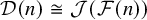 ${\cal D}(n)\cong {\cal J}({\cal F}(n))$
.
${\cal D}(n)\cong {\cal J}({\cal F}(n))$
.
Proof. We have shown that
 ${\cal D}(n)$
and
${\cal D}(n)$
and
 ${\cal J}({\cal F}(n))$
are each isomorphic to a sublattice of
${\cal J}({\cal F}(n))$
are each isomorphic to a sublattice of
 $\{0,1\}^r$
, and these sublattices have the same set of join-irreducible elements. Therefore, these two sublattices coincide.
$\{0,1\}^r$
, and these sublattices have the same set of join-irreducible elements. Therefore, these two sublattices coincide.
For
 $n=10$
, the isomorphism of Theorem 3.16 is obtained by comparing the posets in Figures 3 and 4.
$n=10$
, the isomorphism of Theorem 3.16 is obtained by comparing the posets in Figures 3 and 4.
The corank generating function of
 ${\cal J}({\cal F}(n))$
is
${\cal J}({\cal F}(n))$
is
 $$\begin{align*}\operatorname{\mathrm{crgf}}_n(t) = \sum_{I\in{\cal J}({\cal F}(n))} t^{r-|I|}, \end{align*}$$
where
 $r=|{\cal F}(n)|$
. We can use the previous theorem to express
$r=|{\cal F}(n)|$
. We can use the previous theorem to express
 $h_q(n)$
in terms of this generating function.
$h_q(n)$
in terms of this generating function.
Theorem 3.17. For all
 $n\in {\mathbb N}$
, if
$n\in {\mathbb N}$
, if
 $\beta (n)$
has s ones, then
$\beta (n)$
has s ones, then
 $$ \begin{align} h_q(n) = q^s \operatorname{\mathrm{crgf}}_n(q). \end{align} $$
Proof. Suppose the principal prefix of
 $\beta (n)$
has length r and
$\beta (n)$
has length r and
 $\beta (n)$
has s ones. We have
$\beta (n)$
has s ones. We have
 $$ \begin{align} q^{s}\operatorname{\mathrm{crgf}}_n(q) = \sum_{I\in{\cal J}({\cal F}(n))} q^{r+s-|I|}. \end{align} $$
Applying the isomorphism in Theorem 3.16, we claim that this sum transforms into
 $h_q(n)$
. By the assumptions of the theorem, the element
$h_q(n)$
. By the assumptions of the theorem, the element
 $\beta (n)=\hat {1}(n)$
viewed as a partition in
$\beta (n)=\hat {1}(n)$
viewed as a partition in
 ${\cal D}(n)$
has length s and so contributes
${\cal D}(n)$
has length s and so contributes
 $q^s$
to
$q^s$
to
 $h_q(n)$
. On the other hand,
$h_q(n)$
. On the other hand,
 $\hat {1}(n)$
corresponds to the maximum ideal of
$\hat {1}(n)$
corresponds to the maximum ideal of
 ${\cal F}(n)$
which contains all r elements, so the analogous term in (26) is
${\cal F}(n)$
which contains all r elements, so the analogous term in (26) is
 $q^{r+s-r}=q^s$
. By Lemma 3.1, removing an element from an ideal corresponds to increasing the length of the associated hyperbinary partition by
$q^{r+s-r}=q^s$
. By Lemma 3.1, removing an element from an ideal corresponds to increasing the length of the associated hyperbinary partition by
 $1$
. Therefore, equation (25) holds.
$1$
. Therefore, equation (25) holds.
Using the definition of
 $\operatorname {\mathrm {CW}}_q(n)$
, we deduce the following corollary from the previous theorem.
$\operatorname {\mathrm {CW}}_q(n)$
, we deduce the following corollary from the previous theorem.
Corollary 3.18. Given
 $n\geq 1$
, suppose
$n\geq 1$
, suppose
 $\beta (n-1)$
has
$\beta (n-1)$
has
 $s'$
ones and
$s'$
ones and
 $\beta (n)$
has s ones. Then
$\beta (n)$
has s ones. Then
 $$ \begin{align*}\hspace{150pt} \operatorname{\mathrm{CW}}_q(n) = q^{s'-s} \, \frac{\operatorname{\mathrm{crgf}}_{n-1}(q)}{\operatorname{\mathrm{crgf}}_n(q)}. \hspace{150pt} \end{align*} $$
Corollary 3.18 may be alternately obtained from Theorem 2.3 by using a different interpretation of q-deformed rationals discovered by Morier-Genoud and Ovsienko, as we now explain. Suppose
 $r/s>1$
is a rational number with continued fraction expansion given by equation (4). Let
$r/s>1$
is a rational number with continued fraction expansion given by equation (4). Let
 $N=a_1+\cdots +a_m$
and consider the path graph with N edges on a horizontal line. In groups from left to right, we orient
$N=a_1+\cdots +a_m$
and consider the path graph with N edges on a horizontal line. In groups from left to right, we orient
 $a_1$
edges to the left, then
$a_1$
edges to the left, then
 $a_2$
edges to the right, then
$a_2$
edges to the right, then
 $a_3$
edges to the left, and so on. Finally, we delete the two vertices on the ends to obtain a directed path graph
$a_3$
edges to the left, and so on. Finally, we delete the two vertices on the ends to obtain a directed path graph
 ${\cal G}$
. For example, the
${\cal G}$
. For example, the
 $11$
th Calkin-Wilf number is
$11$
th Calkin-Wilf number is
 $\operatorname {\mathrm {CW}}(11)=5/2$
, which has continued fraction representation
$\operatorname {\mathrm {CW}}(11)=5/2$
, which has continued fraction representation
 $[2,2]$
and the corresponding
$[2,2]$
and the corresponding
 ${\cal G}$
is shown in the top line of Figure 5.
${\cal G}$
is shown in the top line of Figure 5.
The directed graph
 ${\cal G}$
for
${\cal G}$
for
 $r/s=5/2$
and its closure sets.
$r/s=5/2$
and its closure sets.

A subset X of vertices of
 ${\cal G}$
is a closure set if there is no arrow
${\cal G}$
is a closure set if there is no arrow
 $u\rightarrow v$
such that
$u\rightarrow v$
such that
 $u\in X$
and
$u\in X$
and
 $v\notin X$
. Let
$v\notin X$
. Let
 $$ \begin{align*}f_{{\cal G}}(q) = \sum_X q^{|X|} \end{align*} $$
where the sum is over all closure sets X for
 ${\cal G}$
. In Figure 5 the closure sets X of
${\cal G}$
. In Figure 5 the closure sets X of
 ${\cal G}$
are displayed in the last four lines, where a vertex is black or white depending on whether the vertex is or is not in X, respectively. We also consider a subgraph
${\cal G}$
are displayed in the last four lines, where a vertex is black or white depending on whether the vertex is or is not in X, respectively. We also consider a subgraph
 ${\cal G}'$
of
${\cal G}'$
of
 ${\cal G}$
obtained by deleting an additional
${\cal G}$
obtained by deleting an additional
 $a_1$
vertices from the left side of
$a_1$
vertices from the left side of
 ${\cal G}$
. With this setup, [Reference Morier-Genoud and OvsienkoMGO20, Theorem 4] (acknowledging ties with work of Lee and Schiffler [Reference Lee and SchifflerLS19]) states that
${\cal G}$
. With this setup, [Reference Morier-Genoud and OvsienkoMGO20, Theorem 4] (acknowledging ties with work of Lee and Schiffler [Reference Lee and SchifflerLS19]) states that
 $$ \begin{align} \left[\frac{r}{s}\right]_q = \frac{f_{{\cal G}}(q)}{f_{{\cal G}'}(q)}. \end{align} $$
Continuing our example, we see from Figure 5 that
 $f_{{\cal G}}(q) = 1+2q+q^2+q^3$
. The other graph
$f_{{\cal G}}(q) = 1+2q+q^2+q^3$
. The other graph
 ${\cal G}'$
only has one vertex, and
${\cal G}'$
only has one vertex, and
 $f_{{\cal G}'}(q) = 1+q$
. Hence,
$f_{{\cal G}'}(q) = 1+q$
. Hence,
 $[5/2]_q = \frac {1+2q+q^2+q^3}{1+q}$
.
$[5/2]_q = \frac {1+2q+q^2+q^3}{1+q}$
.
To compare (27) with Corollary 3.18, note that the directed graphs
 ${\cal G},{\cal G}'$
can be converted into a fence poset where a directed edge
${\cal G},{\cal G}'$
can be converted into a fence poset where a directed edge
 $u\rightarrow v$
is replaced by a cover
$u\rightarrow v$
is replaced by a cover
 $u\lhd v$
. Under this correspondence, closure sets become order filters, which are in bijection with order ideals by complementation. Thus, each coefficient of the corank generating function of
$u\lhd v$
. Under this correspondence, closure sets become order filters, which are in bijection with order ideals by complementation. Thus, each coefficient of the corank generating function of
 ${\cal J}({\cal F}(n))$
enumerates closure sets of a particular size. Continuing our example, we have
${\cal J}({\cal F}(n))$
enumerates closure sets of a particular size. Continuing our example, we have
 $\operatorname {\mathrm {crgf}}_{10}(q) = 1+2q+q^2+q^3$
from Figure 2. Since
$\operatorname {\mathrm {crgf}}_{10}(q) = 1+2q+q^2+q^3$
from Figure 2. Since
 ${\cal F}(11)$
is a 1-element poset, its lattice of order ideals has corank generating function
${\cal F}(11)$
is a 1-element poset, its lattice of order ideals has corank generating function
 $\operatorname {\mathrm {crgf}}_{11}(q)=1+q$
. Using Theorem 2.3 and then Corollary 3.18, we see that
$\operatorname {\mathrm {crgf}}_{11}(q)=1+q$
. Using Theorem 2.3 and then Corollary 3.18, we see that
 $$\begin{align*}[5/2]_q = [\operatorname{\mathrm{CW}}(11)]_q = q\operatorname{\mathrm{CW}}_q(11) = q\cdot q\: \frac{\operatorname{\mathrm{crgf}}_{10}(q)}{\operatorname{\mathrm{crgf}}_{11}(q)} = \frac{1+2q+q^2+q^3}{1+q} \end{align*}$$
which agrees with the previous computation.
4 Matrices
Consider the matrices
 $$ \begin{align} L = \left[ \begin{array}{cc} 1 & 0\\ 1 & q^{-1} \end{array} \right] \quad\text{and}\quad R = \left[ \begin{array}{cc} q & 1\\ 0 & 1 \end{array} \right]. \end{align} $$
Morier-Genoud and Ovsienko [Reference Morier-Genoud and OvsienkoMGO20] showed that the q-analogues of rational numbers can be expressed as ratios of entries in products involving L and R. In this section, we will relate certain products to hyperbinary partitions. We note that Han et al. [Reference Han, Masuda, Singh and ThielHMST16, Reference Han, Masuda, Singh and ThielHMST20] have studied a generalization of the Calkin-Wilf sequence generated by matrices
 $$ \begin{align*}L_u = \left[ \begin{array}{cc} 1 & 0\\ u & 1 \end{array} \right] \quad\text{and}\quad R_v = \left[ \begin{array}{cc} 1 & v\\ 0 & 1 \end{array} \right]. \end{align*} $$
Define a sequence of matrices
 $M(n)$
for
$M(n)$
for
 $n\ge 1$
as follows. Let the binary expansion of n be
$n\ge 1$
as follows. Let the binary expansion of n be
 $\beta (n)=b_1\ldots b_k$
so that
$\beta (n)=b_1\ldots b_k$
so that
 $b_1=1$
. Removing the initial
$b_1=1$
. Removing the initial
 $1$
and reading the sequence backwards results in
$1$
and reading the sequence backwards results in
 $b_k b_{k-1}\ldots b_2$
. Now let
$b_k b_{k-1}\ldots b_2$
. Now let
 $M(n)$
be the matrix obtained from the product formed by replacing each
$M(n)$
be the matrix obtained from the product formed by replacing each
 $0$
in
$0$
in
 $b_k b_{k-1}\ldots b_2$
by L and each
$b_k b_{k-1}\ldots b_2$
by L and each
 $1$
by R. For example, if
$1$
by R. For example, if
 $n=19$
then
$n=19$
then
 $\beta (19)=10011$
. So, the reversed sequence is
$\beta (19)=10011$
. So, the reversed sequence is
 $1100$
and
$1100$
and
 $$ \begin{align*} M(19) &= RRLL\\ &= \left[ \begin{array}{cc} q & 1\\ 0 & 1 \end{array} \right] \left[ \begin{array}{cc} q & 1\\ 0 & 1 \end{array} \right] \left[ \begin{array}{cc} 1 & 0\\ 1 & q^{-1} \end{array} \right] \left[ \begin{array}{cc} 1 & 0\\ 1 & q^{-1} \end{array} \right] \\[5pt] &= \left[ \begin{array}{cc} q^{-1}+ 2 + q + q^2 & q^{-1} + q^{-2}\\ q^{-1} + 1 & q^{-2} \end{array} \right]. \end{align*} $$
We give a formula for the entries of
 $M(n)$
in Theorem 4.2. First, we compute formulas for
$M(n)$
in Theorem 4.2. First, we compute formulas for
 $h_q(n)$
for certain n in the following lemma.
$h_q(n)$
for certain n in the following lemma.
Lemma 4.1. Let n be such that one has the factorization
 $$ \begin{align*}\beta(n) = ac \end{align*} $$
where
 $a=1^r$
is the principal prefix, and c has at most one zero together with s ones. Then
$a=1^r$
is the principal prefix, and c has at most one zero together with s ones. Then
 $$ \begin{align*}h_q(n)=\left\{\begin{array}{ll}q^{r+s} + q^{r+s+1}+\cdots+q^{2r+s}&\text{if c has a zero,}\\ {q^r}& \text{if c has no zero.}\end{array}\right. \end{align*} $$
Proof. Since a is the principal prefix, the assumptions on c imply that either c is the empty word or
 $c=01^s$
. In the former case,
$c=01^s$
. In the former case,
 $a=1^r$
is the unique hyperbinary expansion of n and has length r. Thus
$a=1^r$
is the unique hyperbinary expansion of n and has length r. Thus
 $h_q(n)=q^r$
.
$h_q(n)=q^r$
.
If
 $c=01^s$
then, from Proposition 3.2, we have
$c=01^s$
then, from Proposition 3.2, we have
 $$ \begin{align*}\hat{1}(n) = \beta(n)=1^r 0 1^s. \end{align*} $$
Now Lemma 3.1 implies that
 ${\cal D}(n)$
is a chain with
${\cal D}(n)$
is a chain with
 $r+1$
elements. Also,
$r+1$
elements. Also,
 $\ell (\hat {1}(n))=r+s$
so this element contributes
$\ell (\hat {1}(n))=r+s$
so this element contributes
 $q^{r+s}$
to
$q^{r+s}$
to
 $h_q(n)$
. By the lemma just cited, length increases by
$h_q(n)$
. By the lemma just cited, length increases by
 $1$
as one goes from an element of
$1$
as one goes from an element of
 ${\cal D}(n)$
to an element it covers. The formula given for
${\cal D}(n)$
to an element it covers. The formula given for
 $h_q(n)$
in this case now follows.
$h_q(n)$
in this case now follows.
For
 $k,l\in {\mathbb N}$
, we use the notation
$k,l\in {\mathbb N}$
, we use the notation
 $$ \begin{align*}[k,l) =\{k,k+1,\ldots,l-1\}. \end{align*} $$
Theorem 4.2. Suppose that
 $n\in [2^{k-1}, 2^k-1)$
and write
$n\in [2^{k-1}, 2^k-1)$
and write
 $\beta (n)=b_1 b_2\ldots ,b_k$
. Let j be the maximum index such that
$\beta (n)=b_1 b_2\ldots ,b_k$
. Let j be the maximum index such that
 $b_1=\ldots =b_j=1$
and define
$b_1=\ldots =b_j=1$
and define
 $n'$
by
$n'$
by
 $$ \begin{align*}\beta(n') = 1 b_{j+2} b_{j+3} \ldots b_k. \end{align*} $$
Then
 $$ \begin{align*}M(n) = \left[ \begin{array}{cc} q^{-k+2j}\ h_q(n' -1) & q^{-k+2}\ h_q(n - 2^{k-1} - 1)\\[5pt] q^{-k+2j-1}\ h_q(n') & q^{-k+1}\ h_q(n - 2^{k-1}) \end{array} \right]. \end{align*} $$
If
 $n=2^k-1$
then the same formula holds with the first column replaced by
$n=2^k-1$
then the same formula holds with the first column replaced by
 $$ \begin{align*}\left[ \begin{array}{c} q^{k-1} \\[5pt] 0 \end{array} \right]. \end{align*} $$
Proof. For each
 $n\ge 1$
, let
$n\ge 1$
, let
 $N(n)$
be the matrix on the right-hand side of the above equation. We prove
$N(n)$
be the matrix on the right-hand side of the above equation. We prove
 $M(n)=N(n)$
by induction on k and divide the proof into four cases.
$M(n)=N(n)$
by induction on k and divide the proof into four cases.
Case 1:
 $n = 2^k-1$
.
$n = 2^k-1$
.
In this case,
 $\beta (n) = 1^k$
, so
$\beta (n) = 1^k$
, so
 $M(n)=R^{k-1}$
. By induction, one can check that
$M(n)=R^{k-1}$
. By induction, one can check that
 $$\begin{align*}R^{k-1} = \begin{bmatrix} q^{k-1} & 1+q+\cdots+q^{k-2}\\ 0 & 1 \end{bmatrix}. \end{align*}$$
Applying the identity
 $n-2^{k-1} = 2^{k-1}-1$
, we have
$n-2^{k-1} = 2^{k-1}-1$
, we have
 $$\begin{align*}N(n) = \begin{bmatrix} q^{k-1} & q^{-k+2} h_q( 2^{k-1}-2 )\\ 0 & q^{-k+1} h_q(2^{k-1} - 1) \end{bmatrix}. \end{align*}$$
Now
 $\beta (2^{k-1}-1)=1^{k-1}$
and
$\beta (2^{k-1}-1)=1^{k-1}$
and
 $\beta (2^{k-1}-2)=1^{k-2}0$
. So, by Lemma 4.1, we deduce
$\beta (2^{k-1}-2)=1^{k-2}0$
. So, by Lemma 4.1, we deduce
 $M(n)=N(n)$
.
$M(n)=N(n)$
.
Case 2:
 $n = 2^k - 2$
.
$n = 2^k - 2$
.
The binary expansion of n is
 $\beta (n)=1^{k-1}0$
, so
$\beta (n)=1^{k-1}0$
, so
 $M(n)=LR^{k-2}$
. From Case 1, we have
$M(n)=LR^{k-2}$
. From Case 1, we have
 $$\begin{align*}M(n) = \begin{bmatrix} 1 & 0\\ 1 & q^{-1} \end{bmatrix} \begin{bmatrix} q^{k-2} & 1 + q+\cdots + q^{k-3}\\ 0 & 1 \end{bmatrix} = \begin{bmatrix} q^{k-2} & 1 + q+\cdots + q^{k-3}\\ q^{k-2} & q^{-1} + 1 + q+\cdots + q^{k-3} \end{bmatrix}. \end{align*}$$
Since there are
 $k-1$
leading
$k-1$
leading
 $1$
’s in the binary expansion of n, we have
$1$
’s in the binary expansion of n, we have
 $j=k-1$
and
$j=k-1$
and
 $n'=1$
. We also have
$n'=1$
. We also have
 $n-2^{k-1} = 2^{k-1}-2$
. Hence,
$n-2^{k-1} = 2^{k-1}-2$
. Hence,
 $$\begin{align*}N(n) = \begin{bmatrix} q^{k-2} h_q(0) & q^{-k+2} h_q(2^{k-1}-3)\\ q^{k-3} h_q(1) & q^{-k+1} h_q(2^{k-1}-2) \end{bmatrix}. \end{align*}$$
We have
 $\beta (2^{k-1}-3)=1^{k-3}01$
and
$\beta (2^{k-1}-3)=1^{k-3}01$
and
 $\beta (2^{k-1}-2)$
from Case 1. Applying Lemma 4.1, we obtain
$\beta (2^{k-1}-2)$
from Case 1. Applying Lemma 4.1, we obtain
 $M(n)=N(n)$
again.
$M(n)=N(n)$
again.
Case 3:
 $n\in [2^{k-1},2^k-2)$
and n is odd.
$n\in [2^{k-1},2^k-2)$
and n is odd.
Let
 $m\in {\mathbb N}$
such that
$m\in {\mathbb N}$
such that
 $n=2m+1$
. Then
$n=2m+1$
. Then
 $\beta (n)=b_1\ldots b_{k-1}1$
and
$\beta (n)=b_1\ldots b_{k-1}1$
and
 $\beta (m)=b_1\ldots b_{k-1}$
. Hence,
$\beta (m)=b_1\ldots b_{k-1}$
. Hence,
 $M(n) = R\cdot M(m)$
.
$M(n) = R\cdot M(m)$
.
Since
 $\beta (n)\ne 1^k$
, the words
$\beta (n)\ne 1^k$
, the words
 $\beta (n)$
and
$\beta (n)$
and
 $\beta (m)$
have the same number of leading
$\beta (m)$
have the same number of leading
 $1$
’s. In particular, we have
$1$
’s. In particular, we have
 $n' = 2m' +1$
. Since
$n' = 2m' +1$
. Since
 $m\in [2^{k-2},2^{k-1}-1)$
we may apply the inductive hypothesis to get
$m\in [2^{k-2},2^{k-1}-1)$
we may apply the inductive hypothesis to get
 $$ \begin{align*} M(n) &= \begin{bmatrix} q & 1\\ 0 & 1 \end{bmatrix} \begin{bmatrix} q^{-k+2j+1}h_q(m'-1) & q^{-k+3} h_q(m-2^{k-2}-1)\\ q^{-k+2j}h_q(m') & q^{-k+2} h_q(m-2^{k-2}) \end{bmatrix}\\[10pt] &= \begin{bmatrix} q^{-k+2j+2}h_q(m'-1) + q^{-k+2j}h_q(m') & q^{-k+4}h_q(m-2^{k-2}-1)+q^{-k+2}h_q(m-2^{k-2})\\ q^{-k+2j}h_q(m') & q^{-k+2}h_q(m-2^{k-2}) \end{bmatrix}\\[10pt] &= \begin{bmatrix} q^{-k+2j}h_q(2m') & q^{-k+2} h_q(2m-2^{k-1})\\ q^{-k+2j-1}h_q(2m'+1) & q^{-k+1} h_q(2m-2^{k-1}+1) \end{bmatrix} \end{align*} $$
where the last equation follows by applying Proposition 2.2. Using the substitutions
 $n=2m+1$
and
$n=2m+1$
and
 $n'=2m'+1$
, we conclude
$n'=2m'+1$
, we conclude
 $M(n)=N(n)$
.
$M(n)=N(n)$
.
Case 4:
 $n\in [2^{k-1},2^k-2)$
and n is even.
$n\in [2^{k-1},2^k-2)$
and n is even.
The proof in this case is very similar to the proof of Case 3, starting with
 $n=2m,\ n'=2m'$
, and
$n=2m,\ n'=2m'$
, and
 $M(n)=L\cdot M(m)$
. Due to the similarity to Case 3, we omit the proof.
$M(n)=L\cdot M(m)$
. Due to the similarity to Case 3, we omit the proof.
The row sums of
 $M(n)$
take a particularly nice form. This result can be derived as a corollary of Theorem 4.2, but we give a simpler proof using the definition of
$M(n)$
take a particularly nice form. This result can be derived as a corollary of Theorem 4.2, but we give a simpler proof using the definition of
 $M(n)$
and the recurrence in Proposition 2.2.
$M(n)$
and the recurrence in Proposition 2.2.
Theorem 4.3. If
 $n\in [2^{k-1},2^k)$
then
$n\in [2^{k-1},2^k)$
then
 $$ \begin{align*}M(n) \left[ \begin{array}{c} 1\\[5pt] 1 \end{array} \right] = \left[ \begin{array}{c} q^{-k+1}\ h_q(n-1)\\[5pt] q^{-k}\ h_q(n) \end{array} \right]. \end{align*} $$
Proof. As usual, we induct on n where there are two cases depending on parity. We will only do the even case as the odd case is similar. Since
 $2^{k-1}$
is the largest power of
$2^{k-1}$
is the largest power of
 $2$
less than or equal to n, we have
$2$
less than or equal to n, we have
 $\beta (n)=b_1\ldots b_k$
and
$\beta (n)=b_1\ldots b_k$
and
 $\beta (2n)= \beta (n) 0$
. Transforming this into matrices we see that we have
$\beta (2n)= \beta (n) 0$
. Transforming this into matrices we see that we have
 $M(2n) = L M(n)$
. It follows from induction and Proposition 2.2 that
$M(2n) = L M(n)$
. It follows from induction and Proposition 2.2 that
 $$ \begin{align*} M(2n) \left[ \begin{array}{c} 1\\[5pt] 1 \end{array} \right] & =L M(n) \left[ \begin{array}{c} 1\\[5pt] 1 \end{array} \right] \\[5pt] &= \left[ \begin{array}{cc} 1 & 0\\ 1 & q^{-1} \end{array} \right] \left[ \begin{array}{c} q^{-k+1}\ h_q(n-1)\\[5pt] q^{-k}\ h_q(n) \end{array} \right] \\[5pt] &= \left[ \begin{array}{c} q^{-k+1}\ h_q(n-1)\\[5pt] q^{-k+1}\ h_q(n-1)+q^{-k-1}\ h_q(n) \end{array} \right] \\[5pt] &= \left[ \begin{array}{c} q^{-k}\ h_q(2n-1)\\[5pt] q^{-k-1}\ h_q(2n) \end{array} \right] \end{align*} $$
as desired.
We can derive a 2-variable analogue of Theorem 4.3 as follows. Let
 $r,s$
be two indeterminates and define
$r,s$
be two indeterminates and define
 $$ \begin{align*}L' = \left[ \begin{array}{cc} 1 & 0\\ r & s \end{array} \right] \quad\text{and}\quad R' = \left[ \begin{array}{cc} r & s\\ 0 & 1 \end{array} \right]. \end{align*} $$
Also let
 $M'(n)$
be the matrix obtained from the
$M'(n)$
be the matrix obtained from the
 $L,R$
product for
$L,R$
product for
 $M(n)$
by replacing each L by
$M(n)$
by replacing each L by
 $L'$
and each R by
$L'$
and each R by
 $R'$
. As for the hyperbinary polynomials, given a hyperbinary expansion
$R'$
. As for the hyperbinary polynomials, given a hyperbinary expansion
 $d=d_1d_2\ldots d_k$
for n we consider the statistics
$d=d_1d_2\ldots d_k$
for n we consider the statistics
 $$ \begin{align*}t(d) = \text{number of twos in }d, \end{align*} $$
and
 $$ \begin{align*}z(d) = \text{numbers of nonleading zeros in }d, \end{align*} $$
that is, the number of zeros to the right of the leftmost nonzero digit of d. For example, if
 $n=34$
and
$n=34$
and
 $d=020010$
then
$d=020010$
then
 $t(d)=1$
and
$t(d)=1$
and
 $z(d)=3$
. Define the generating function
$z(d)=3$
. Define the generating function
 $$ \begin{align*}H_{rs}(n) = \sum_{d\in{\cal D}(n)} r^{t(d)} s^{z(d)}. \end{align*} $$
The proof of the following result is much the same as the demonstrations of Proposition 2.2 and Theorem 4.3 and so is omitted.
Theorem 4.4. We have
 $h_{rs}(-1)=0$
,
$h_{rs}(-1)=0$
,
 $h_{rs}(0) = 1$
, and for
$h_{rs}(0) = 1$
, and for
 $n\ge 1$
 $$ \begin{align} h_{rs}(2n-1) &= h_{rs}(n-1), \end{align} $$
 $$ \begin{align} h_{rs}(2n) &= s h_{rs}(n) + r h_{rs}(n-1). \end{align} $$
For all
 $n\ge 0$

Of course, we could combine all three statistics,
 $\ell (d)$
,
$\ell (d)$
,
 $t(d)$
, and
$t(d)$
, and
 $z(d)$
. The reader should be able to supply the details.
$z(d)$
. The reader should be able to supply the details.
5 Comments and future work
We gather here various ideas for future work and open problems.
5.1 Negative numbers
In the context of the q-deformed rationals, it is very natural to include negative rationals along with positive ones. One can devise two-sided Stern sequences
 $$ \begin{align*}\dots -1, 3, -2, 3, -1, 2, -1, 1, 0, 1, 1, 2, 1, 3, 2, 3, 1, \dots\end{align*} $$
and
 $$ \begin{align*}\dots 1, -3, 2, -3, 1, -2, 1, -1, 0, 1, 1, 2, 1, 3, 2, 3, 1, \dots,\end{align*} $$
either of which will allow us to obtain every rational number (along with the honorary number
 $\infty $
) as a quotient of successive terms, but is there a rationale for either of these artificial-seeming sequences?
$\infty $
) as a quotient of successive terms, but is there a rationale for either of these artificial-seeming sequences?
Perhaps a clue comes from the 2-adic numbers. In this context,
 $-1$
can be represented through the left-infinite digit-sequence
$-1$
can be represented through the left-infinite digit-sequence
 $\cdots 111$
. Might such representations provide a hint?
$\cdots 111$
. Might such representations provide a hint?
5.2 Lattices
As illustrated at the beginning of Section 3, the set of all partitions of n do not form a lattice under refinement for
 $n\ge 5$
. But the subset of hyperbinary partitions does and, in fact, the lattice is distributive. It would be interesting to identify other natural subposets of the full partition poset which are lattices and satisfy various lattice properties.
$n\ge 5$
. But the subset of hyperbinary partitions does and, in fact, the lattice is distributive. It would be interesting to identify other natural subposets of the full partition poset which are lattices and satisfy various lattice properties.
5.3 Other statistics
At the end of Section 4 we indicated how a couple of our results could be modified using two other statistics. It would be interesting to see whether other theorems in this work have such analogues. Also there are other statistics that could be studied.
As another example, given a hyperbinary partition
 $\eta $
we let
$\eta $
we let
 $$ \begin{align*}p_i(\eta) = \text{number of parts of }\eta\text{ of multiplicity }i \end{align*} $$
for
 $i = 1, 2$
. In Section 4 we used the notation
$i = 1, 2$
. In Section 4 we used the notation
 $t(\eta )=p_2(\eta )$
. As an alternative description, suppose that
$t(\eta )=p_2(\eta )$
. As an alternative description, suppose that
 $\eta $
is written out in terms of its digits in hyperbinary
$\eta $
is written out in terms of its digits in hyperbinary
 $d=d_1 d_2\ldots d_k$
. Then
$d=d_1 d_2\ldots d_k$
. Then
 $$ \begin{align*}p_i(\eta) = \text{number of digits in }d\text{ equal to }i. \end{align*} $$
Note that we have the relation
 $$ \begin{align} \ell(\eta) = p_1(\eta) + 2p_2(\eta). \end{align} $$
The statistics
 $p_1$
and
$p_1$
and
 $p_2$
, have been considered, respectively, by Klavžar, Milutinović, and Petr [Reference Klavžar, Milutinović and PetrKMP07] and by Bates and Mansour [Reference Bates and MansourBM11]. As far as we know our statistic
$p_2$
, have been considered, respectively, by Klavžar, Milutinović, and Petr [Reference Klavžar, Milutinović and PetrKMP07] and by Bates and Mansour [Reference Bates and MansourBM11]. As far as we know our statistic
 $\ell $
has not been studied before, although it is the one most closely related to the q-rationals of Morier-Genoud and Ovsienko.
$\ell $
has not been studied before, although it is the one most closely related to the q-rationals of Morier-Genoud and Ovsienko.
Consider the generating function
 $$ \begin{align*}\overline{h}_{s,t}(n) = \sum_{\eta\in H(n)} s^{p_1(\eta)} t^{p_2(\eta)}. \end{align*} $$
Using (31) we see that setting
 $s=q$
and
$s=q$
and
 $t=q^2$
recovers our previously considered polynomial
$t=q^2$
recovers our previously considered polynomial
 $h_q(n) = \sum _{\eta \in H(n)} q^{\ell (\eta )}$
. The next result is derived from Proposition 2.1 in much the same way as Proposition 2.2, so we omit the details.
$h_q(n) = \sum _{\eta \in H(n)} q^{\ell (\eta )}$
. The next result is derived from Proposition 2.1 in much the same way as Proposition 2.2, so we omit the details.
Proposition 5.1. We have
 $\overline {h}_{s,t}(0) = 1$
, and for
$\overline {h}_{s,t}(0) = 1$
, and for
 $n\ge 1$
 $$ \begin{align*} \overline{h}_{s,t}(2n-1) &= s\overline{h}_{s,t}(n-1),\\ \hspace{140pt} \overline{h}_{s,t}(2n) &= \overline{h}_{s,t}(n) + t\overline{h}_{s,t}(n-1).\hspace{140pt} \end{align*} $$
In [Reference Mansour and ShattuckMS11], Mansour and Shattuck studied the statistics
 $p_2(\eta )$
and
$p_2(\eta )$
and
 $$ \begin{align*}d(\eta)= \text{ number of distinct parts of }\eta, \end{align*} $$
that is, the number of nonzero digits in the hyperbinary expansion corresponding to
 $\eta $
. Note that
$\eta $
. Note that
 $$ \begin{align*}\ell(\eta)=d(\eta)+ p_2(\eta). \end{align*} $$
Among other things, they derived an analogue of Theorem 2.3 for a different q-analogue of
 $\operatorname {\mathrm {CW}}(n)$
. Mansour and Shattuck also studied additional parameters and an extension to m-ary partitions in [Reference Mansour and ShattuckMS15]. In [Reference MansourMan15], Mansour considered polynomials which are, up to a shift of indices, the
$\operatorname {\mathrm {CW}}(n)$
. Mansour and Shattuck also studied additional parameters and an extension to m-ary partitions in [Reference Mansour and ShattuckMS15]. In [Reference MansourMan15], Mansour considered polynomials which are, up to a shift of indices, the
 $\overline {h}_{s,t}(n)$
. He shows that they are related to continued fractions similar to those studied by Morier-Genoud and Ovsienko, but only giving the numerators.
$\overline {h}_{s,t}(n)$
. He shows that they are related to continued fractions similar to those studied by Morier-Genoud and Ovsienko, but only giving the numerators.
A different statistic was studied by Dilcher and Ericksen [Reference Dilcher and EricksenDE15], as well as by Dilcher and Stolarsky [Reference Dilcher and StolarskyDS07]; their statistic reduces each nonzero digit by 1 and interprets the result in binary.
5.4 Chip firing
Another perspective that might give rise to analogues of our theorems is the chip-firing perspective. One can regard the hyperbinary expansion
 $d_1 d_2 \dots d_k$
of a number as configurations of chips on the natural numbers, with
$d_1 d_2 \dots d_k$
of a number as configurations of chips on the natural numbers, with
 $d_i$
chips residing at the location
$d_i$
chips residing at the location
 $k-i$
, where a chip-firing move replaces 2 chips at m by 1 chip at
$k-i$
, where a chip-firing move replaces 2 chips at m by 1 chip at
 $m+1$
, where a site with 3 or more chips must fire and a site with 2 chips may fire. Although our write-up does not mention chips explicitly, we found the perspective a helpful source of intuition. Other chip-games might have similar properties. Richard Stanley (in private communication) proposes a generalization in which no location can have more than r chips, and each chip divides into s chips when it moves one step to the right.
$m+1$
, where a site with 3 or more chips must fire and a site with 2 chips may fire. Although our write-up does not mention chips explicitly, we found the perspective a helpful source of intuition. Other chip-games might have similar properties. Richard Stanley (in private communication) proposes a generalization in which no location can have more than r chips, and each chip divides into s chips when it moves one step to the right.
Acknowledgments
The authors acknowledge helpful suggestions from Neil Calkin, Sophie Morier-Genoud, Valentin Ovsienko, Bruce Reznick, Richard Stanley, Günter Ziegler, and the two anonymous referees.
Competing interest
The authors have no competing interests to declare.
Financial support
None.


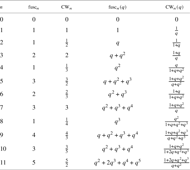


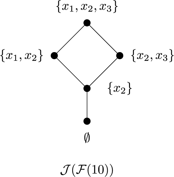

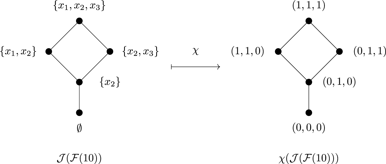


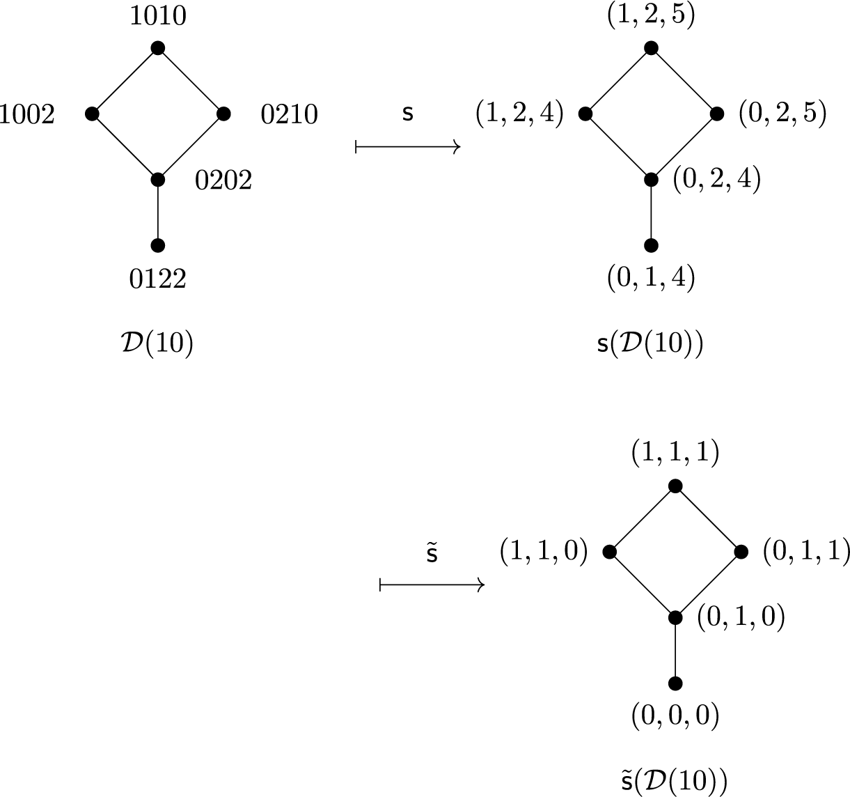


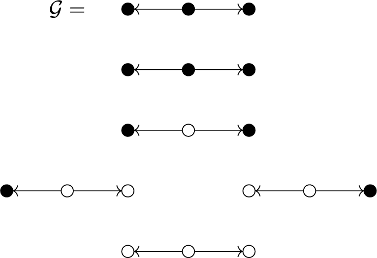


 Open access