


Non-technical Summary
At the end of the last ice age, there was a major worldwide shift in climate, and animals may have had to adapt to the changes in order to survive. Many modern animals are larger and stockier in parts of their range with colder climates, so we might expect Ice Age animals to be larger and stockier than their relatives living in a warmer, more modern climate. The fossils at Rancho La Brea formed during this time, so we can test this hypothesis by comparing older La Brea fossils to newer ones. However, this requires accurate estimates of their ages, which can be complicated, because each tar pit contains a mixture of older and younger fossils. We have already taken measurements on a large number of fossils from many species. In this paper, we test a new method for estimating population average sizes over time, based on all the radiocarbon dates from each pit.
Our results show that most of the birds and mammals at Rancho La Brea did not change much as the climate warmed, and those that did change size or shape did not all get smaller or change size at the same time that the climate was changing. Using our new method produced some new results that we missed the first time, but that other authors had noticed.
Introduction
Punctuated Equilibrium, Stasis, and the Last Glacial Maximum (LGM)
One of Darwin’s fundamental insights, gained primarily through observations of modern populations, is that the frequencies of traits in populations change in response to their environments. How quickly and when they respond, though, is a question best answered with the fossil record. One of the major shifts in paleontological thinking about the tempo and mode of evolution, initiated 50 years ago, forms the topic of this issue (Eldredge and Gould Reference Eldredge, Gould and Schopf1972; Gould and Eldredge Reference Gould and Eldredge1993). The key to the punctuated equilibrium model of evolution is the observation that evolutionary change in populations is relatively rare, even during intervals of environmental change, and occurs mainly during speciation. This offered a possible solution to the apparent “paradox of stasis,” in which evolution appeared to be rapid and common in living populations, but much slower and rarer on paleontological timescales (e.g., Estes and Arnold Reference Estes and Arnold2007). Indeed, the Pleistocene glacial–interglacial cycles furnish one of the first examples of paleontological stasis noted in print, shortly after the publication of On the Origin of Species: “If we cast a glance back on the long vista of physical changes which our planet has undergone since the Neozoic Epoch, we can nowhere detect signs of a revolution more sudden and pronounced, and more important in its results, than the intercalation and subsequent disappearance of the Glacial period. Yet the mammoth lived before it, and passed through the ordeal of all the hard extremities which it involved, bearing his organs of locomotion and digestion all but unchanged” (Falconer Reference Falconer1863: p. 44). In creating a theoretical framework for interpreting stasis, however, Eldredge and Gould invited paleontologists to investigate it explicitly and interpret their results in terms that explored the concept of tempo variation and timescale dependency in evolution.
Paleontologists’ discussion of variations in the tempo and mode of evolution has by now transcended simple comparison of the relative frequencies of gradual versus punctuated change; modern studies are more likely to address the temporal scaling of evolutionary change in general, using a variety of new analytical techniques. As predicted by Stanley (Reference Stanley1975), Vrba and Gould (Reference Vrba and Gould1986), Gould (Reference Gould2002), and Jablonski (Reference Jablonski2008), species rarely show gradual directional change over million-year timescales. Although ephemeral evolutionary change is common and uncorrelated with time on sub-million-year timescales, phenotypic changes rarely persist and accumulate for much longer than that (Estes and Arnold Reference Estes and Arnold2007; Uyeda et al. Reference Uyeda, Hansen, Arnold and Pienaar2011). This discontinuity between short and long timescales has been explained at a population genetics level by the failure of most adaptations to sweep through populations before the local optimum shifts away from them again, unless reproductive isolation allows them to become fixed in a new species. This pattern is termed “ephemeral divergence” by Futuyma (Reference Futuyma2010), who suggests that it may account for the observed association between climatic fluctuation and morphological stasis.
Ecological niche occupation traits appear to be at least as conservative as morphological traits; documented examples of niche shift are exceedingly rare, even during speciation events. Results from ecological niche model studies indicate that environmental changes on sub-million-year timescales usually result only in range shifts, even in lineages that split by environmentally driven vicariant or allopatric speciation. Climatic niches are highly phylogenetically conserved: little niche shift occurs on the 10³–10⁴ year timescale, either during speciation events (Wiens Reference Wiens2004; Peterson Reference Peterson2011; Pyron et al. Reference Pyron, Costa, Patten and Burbrink2015) or after several million years of separation between sister species, with significant niche shift occurring only after an order of magnitude longer (Peterson et al. Reference Peterson, Soberón and Sánchez-Cordero1999). Even in a case where genetic data indicate intraspecific evolution with a large subspecies being replaced by a small one during the Pleistocene/Holocene transition, ecological niche modeling indicates that climate was probably not the cause (Prost et al. Reference Prost, Klietmann, van Kolfschoten, Guralnick, Waltari, Vrieling and Stiller2013).
The apparent paradox of the lack of change on the sub-million-year timescales, but the many examples of change on the multi-million-year timescale, can best be explained by species sorting in both clades and assemblages (Prothero et al. Reference Prothero, Syverson, Raymond, Madan, Molina, Fragomeni, DeSantis, Sutyagina and Gage2012). Studies that demonstrate apparent change in species with climate over multi-million-year timescales (Janis Reference Janis1989, Reference Janis1993; Stucky Reference Stucky, Prothero and Berggren1992; Prothero Reference Prothero1999) treat species as discrete units with static properties and sum the species diversity (treated as discrete units with their own properties) in bins of 2–3 Myr in duration or longer, so they are unable to see the fine-scale stasis observed on sub-million-year timescales. The apparent climatic response of species in these multi-million-year studies is not direct morphological change tracking climate on short timescales, but the increase and decrease in number of species in each time bin.
In the light of these insights about the time-scaling of evolutionary change, widespread morphological stasis in vertebrates during the ~105 years of the Pleistocene/Holocene transition is unsurprising, and ecological stasis is exactly what would be expected. Studies in a variety of taxa back this prediction, including mammals (e.g., Barnosky Reference Barnosky2005); birds (e.g., Zink et al. Reference Zink, Klicka and Barber2004); plants (e.g., Willis et al. Reference Willis, Bennett, Walker, Willis and Niklas2004); and reptiles, amphibians, and fishes (Avise et al. Reference Avise, Walker and Johns1998). The results from climatic niche–based species distribution models instead predict that the changes in climatic suitability since the last interglacial (LIG, ~120 ka) should be accommodated by range shifts (Graham et al. Reference Graham, Lundelius, Graham, Schroeder, Toomey, Anderson and Barnosky1996), with most extirpated species being replaced by ecologically similar relatives (McGill et al. Reference McGill, Hadly and Maurer2005).
Tempo and Mode at Rancho La Brea (RLB)
The fossils from the famous tar pit Lagerstätte at RLB provide an opportunity to study the pace of adaptation to environmental change on the 10–100 kyr timescale in an unusually rich and well-preserved Late Pleistocene to Holocene fossil vertebrate fauna. These deposits formed in an asphalt seep in the Los Angeles Basin in Southern California over the last ~50 kyr (Fox et al. Reference Fox, Southon, Howard, Takeuchi, Potze, Farrell, Lindsey and Blois2023), which spans the last full interglacial–glacial cycle of the Pleistocene and the entirety of the Holocene, and preserve a wide range of vertebrates, insects, and plants. The regional vegetation reflects the Pleistocene/Holocene climate transition, shifting from oak–chaparral at the LIG to juniper–pine forest at the LGM and back to oak–chaparral in the Holocene (Heusser Reference Heusser1998; Heusser et al. Reference Heusser, Kirby and Nichols2015). Thus, RLB provides a detailed record of exactly the sort of sub-million-year climatic variability that is thought to produce ephemeral evolutionary change in morphological traits.
Ecological niche conservatism has been specifically documented in the vertebrate fauna of RLB. Ecological niche models of extant bird species found as fossils at RLB indicate that their environmental preferences and life histories have changed minimally since the LGM: niche models based on modern occurrence data predicted the presence at 21 ka of 95% of the species within 100 km of RLB (Zink et al. Reference Zink, Botero-Cañola, Martinez and Herzberg2020). Likewise, dietary isotope data indicate that the diets of RLB fossil individuals of extant mammal species from the LIG are similar to those of their modern conspecifics; Canis latrans, with its unusual dietary flexibility, is the exception that proves the rule (Fuller et al. Reference Fuller, Southon, Fahrni, Farrell, Takeuchi, Nehlich, Guiry, Richards, Lindsey and Harris2020). Obviously, neither of these studies was suitable for examination of extinct species, but both indicate that surviving species inhabit a similar niche to their end-Pleistocene relatives.
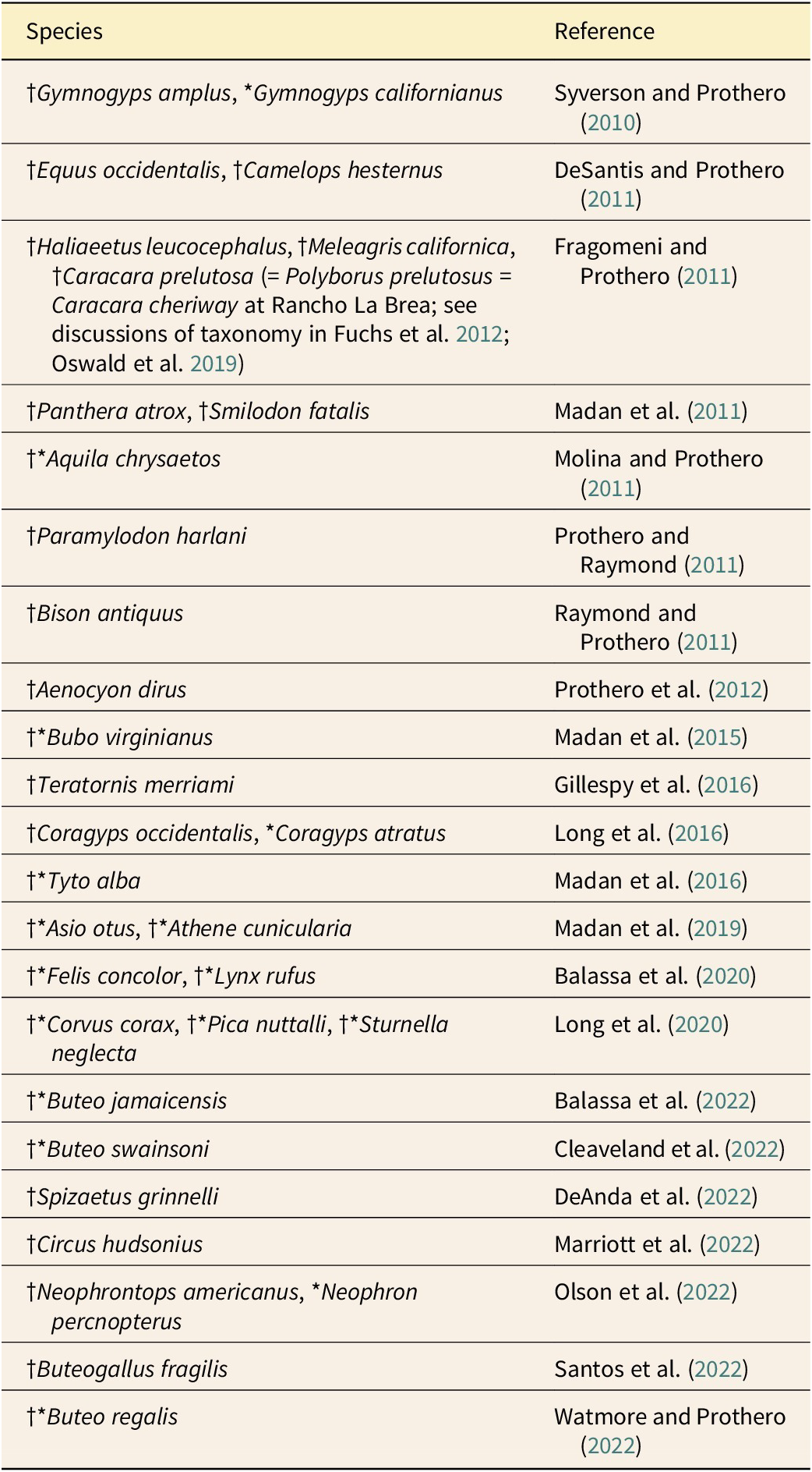
The authors of this paper and our collaborators have published 22 separate papers on individual species or small groups of similar species (Table 1) based on the radiocarbon ages and paleoclimate proxies that were available when we began the project. In 2012, we reviewed the results from the first 12 species we studied (Prothero et al. Reference Prothero, Syverson, Raymond, Madan, Molina, Fragomeni, DeSantis, Sutyagina and Gage2012), finding an overwhelming signal of morphological stasis. Since then, we have measured elements of 23 more species, mostly birds, all with similar results. Over the same period, however, many more RLB radiocarbon dates and regional paleoclimate datasets have been published, as well as a convincing argument against the validity of using pit mean ages (Fuller et al. Reference Fuller, Fahrni, Harris, Farrell, Coltrain, Gerhart, Ward, Taylor and Southon2014). In the present study, we use a newly revised radiocarbon chronology for RLB, a newly revised paleoclimate interpretation for the Los Angeles Basin, and our previously published morphometric datasets to assess whether size or robustness in the vertebrate fossils of RLB can be correlated with the changes in regional climate during the last glacial–interglacial interval.
Species previously published on as part of this series of studies, in order of publication date. Daggers (†) indicate species represented in study by fossil specimens from La Brea Tar Pits Museum; asterisks (*) indicate species in study represented by modern specimens from other collections.
The purpose of the present study is a review and extended correction to this series of papers, in which we reevaluate all parts of the preceding studies. The hypothesis and underlying theory are reevaluated in this section; the suitability and quality of the data are discussed in the next section, along with a reconsideration of the analytical methods and statistical framework. The results of the analysis and our conclusions, therefore, also inevitably demanded a reassessment. The ensuing sections provide a general interpretation of the contribution that we hope to make to the discussion of tempo and mode in evolution by this intensive focus on the relationship between climate and vertebrate body size in the RLB paleoecosystem.
Hypotheses and Predictions
Any study based on a single locality can necessarily only detect local trends. Thus, we may potentially distinguish change from stasis in the local population with this dataset, but we cannot tell range shifts among populations apart from species-level evolutionary change. As such, we must stick to the question of whether the bird and mammal populations at RLB exhibited any morphological response to the climate transition; we cannot claim to evaluate whether that morphological response, be it stasis or change, is a biogeographic or an evolutionary one. Based on the studies already highlighted, we predict that we will not see significant morphological change in most populations.
In recent meta-analyses of evolutionary mode, directional evolution was most strongly supported for between 9% (Hunt et al. Reference Hunt, Hopkins and Lidgard2015) and 14% (Voje Reference Voje2016) of fossil time series. Based on this result, if all the time series were independent, we would expect to find directional evolution in between 40 and 63 of our 455 morphometric measurements (Supplementary Table A). However, our data are likely to be autocorrelated, because they have a great deal of structure: these 455 time series were measured from 57 skeletal elements across 30 species, all from the same set of 26 pit deposits. Comparison to a numeric estimate based on compilations of independent fossil time series from various taxa and intervals is therefore probably not useful. Instead, we should be looking for clusters of directional evolutionary trends that follow the structure of the data. For example, we might expect to find multiple bones with similar trends in a single species; ecologically similar species might all remain stable or change together.
Modern zoology supplies us with a prediction for the timing and direction of any changes we might find, based on known climate-related body-size and body-shape clines in extant populations of a number of RLB species and their close relatives. One of the most commonly recognized of these, Bergmann’s rule, describes a pattern of larger and stockier individuals in cold-adapted populations and smaller, longer-limbed individuals in warmer regions (Mayr Reference Mayr1956). The list of species in which the effect of Bergmann’s rule has been observed includes various extant ungulates (Nowak Reference Nowak1999), felids (Sunquist and Sunquist Reference Sunquist and Sunquist2002), birds of prey (Johnsgard Reference Johnsgard1990), and passerines (Gill Reference Gill2003; Fan et al. Reference Fan, Cai, Xiong, Song and Lei2019), as well as some fossil species such as the Paleogene equid Sifrhippus (Secord et al. Reference Secord, Bloch, Chester, Boyer, Wood, Wing, Kraus, McInerney and Krigbaum2012) and the Late Pleistocene to Holocene woodrat Neotoma cinerea (Smith et al. Reference Smith, Betancourt and Brown1995). Several separate studies have estimated that Bergmann’s rule applies to around 70% of living mammal species, more strongly at higher latitudes (Ashton et al. Reference Ashton, Tracy and de Queiroz2000; Rodríguez et al. Reference Rodríguez, Olalla-Tárraga and Hawkins2008). However, carnivorans in general may not follow it (Yom-Tov and Geffen Reference Yom-Tov and Geffen2011). Indeed, two geometric morphometric studies of RLB carnivorans did not recover this pattern across time: postcranial elements in Canis latrans decrease in size in apparent response to the megafaunal extinction, not to deglaciation (Meachen and Samuels Reference Meachen and Samuels2012), and mandible size in Smilodon fatalis at RLB actually inverts the pattern, with smaller ancestral forms in cold intervals and larger derived forms in warmer times (Meachen et al. Reference Meachen, O’Keefe and Sadler2014). Still, Bergmann’s rule furnishes a reasonable starting point for what overall direction and timing of change, if any, we might expect to see in our RLB vertebrate morphological data.
Data and Methods
No original data were collected for this study. Instead, we used a novel method to assign ages to already-measured specimens, then modeled the evolutionary dynamics of the resulting time series. The overall procedure for this study was as follows: (1) Morphometric data for various RLB vertebrates were compiled from the results of our 22 previous studies. (2) We compiled a database of RLB radiocarbon dates and used it to estimate an age probability distribution for each pit. (3) Each specimen was then assigned an age drawn at random from the appropriate pit age distribution; this step was repeated 1000 times. (4) Time bins were determined based on a variety of regional climate reconstructions. The mean and variance of each measured parameter was then calculated for each time bin. (5) From these, we constructed a time series for each measurement. (6) Finally, a set of evolutionary models was tested against each time series. The following subsections describe each of these steps in detail.
Morphometric Data
Linear measurements of skeletal elements for a variety of the most common vertebrate species found in the RLB asphalt deposits were taken over the course of 12 years by 13 different investigators, using digital or dial calipers. The species and bones measured, counts, and original publications are listed in Supplementary Table A. These include 17 bird and 9 mammal species, of which 14 are extant and 12 extinct. All skeletal elements with 10 or more specimens available were measured. For 10 species, multiple elements were available, but for the majority of bird species this meant only the tarsometatarsus (TMT). The number of individual bones measured from each species ranges from 21 (Pica nuttalli) to 1496 (Smilodon fatalis), and the number of specimens of each skeletal element ranges from 10 (tooth M1 of Puma concolor) to 373 (astragalus of S. fatalis). The measurements taken on each element were chosen to best capture variability in body size and are documented in detail in the original papers (Table 1). For this study, to facilitate comparisons between elements and species, we also log-transformed the data and then did a principal components analysis. The signs of the principal component (PC) rotation matrices were flipped to orient them to the measurements so that the positive direction of each PC corresponded to the positive direction of the measurements. The variation captured in the first two PCs varies from 50% to 100% (scree box plot: Supplementary Fig. B).
The question addressed in this series of studies has been whether climate changes have affected body size or shape in the RLB population of each species. A number of the papers have used measurements of modern conspecifics from zoological collections for comparison. However, the original authors measured recent specimens collected from a variety of different locations and held in a number of different repositories, and many did not record the information necessary to determine whether they were collected in Southern California. The differences between the modern climates of various collection areas very well may eclipse those between glacial and interglacial RLB, so this risks obscuring the signal of any potential population-level effect of climate on morphology. In the present study, we therefore omit modern specimens from all quantitative analyses.
Radiocarbon Estimation of Pit Ages
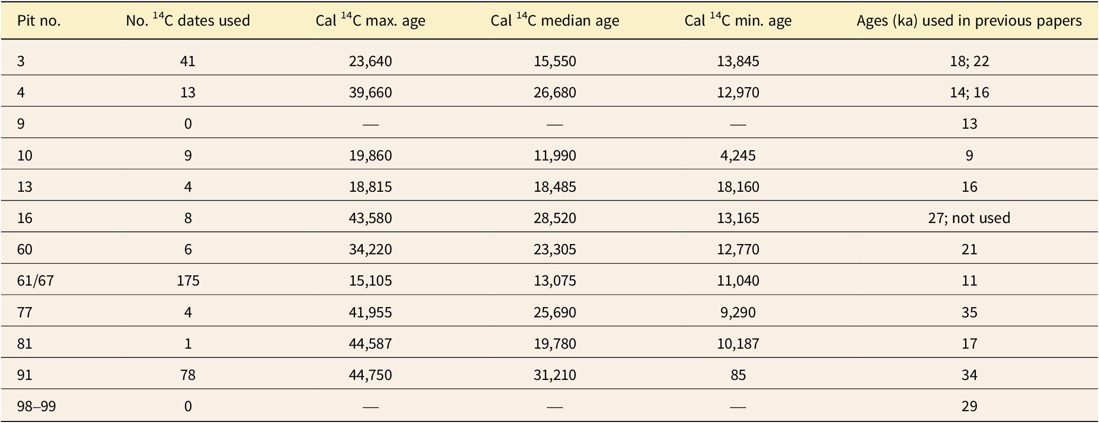
Our previous studies used the RLB ¹⁴C pit ages reported by Marcus and Berger (Reference Marcus, Berger, Martin and Klein1984) and O’Keefe et al. (Reference O’Keefe, Fet and Harris2009), later adding those compiled by Fuller et al. (Reference Fuller, Fahrni, Harris, Farrell, Coltrain, Gerhart, Ward, Taylor and Southon2014, Reference Fuller, Harris, Farrell, Takeuchi, Southon and Harris2015). We then assigned the age of all specimens within a pit to the mean age of that pit. The ages used in these previous studies are given in Table 2. However, as discussed by Fuller et al. (Reference Fuller, Fahrni, Harris, Farrell, Coltrain, Gerhart, Ward, Taylor and Southon2014), this is not good statistical practice, owing to the unusual taphonomic characteristics of the RLB pit deposits. Each “pit” is a single seep of asphalt, a few meters wide and a few meters deep. Within each pit, severe taphonomic time averaging has taken place: vertical relationships between the specimens in a pit have no significance for superposition, and therefore no stratigraphic sequence can be established (Woodard and Marcus Reference Woodard and Marcus1973; Friscia et al. Reference Friscia, Van Valkenburgh, Spencer and Harris2008; O’Keefe et al. Reference O’Keefe, Fet and Harris2009). Each pit must therefore be treated as a single time-averaged deposit. Furthermore, each pit may document multiple disjoint intervals of deposition with irregularly varying intensity, depending on factors such as asphalt flow and surface temperature (Friscia et al. Reference Friscia, Van Valkenburgh, Spencer and Harris2008; Fuller et al. Reference Fuller, Fahrni, Harris, Farrell, Coltrain, Gerhart, Ward, Taylor and Southon2014). The mean age of the specimens in a pit therefore may bear little relation to the age of any individual specimen (Fuller et al. Reference Fuller, Fahrni, Harris, Farrell, Coltrain, Gerhart, Ward, Taylor and Southon2014), which makes it an unsuitable estimator for measurements taken from individual specimens.
Median and boundary (95% CI) radiocarbon ages for pits at Rancho La Brea, calculated using OxCal and expressed in calendar years BP, along with the age values used in the previous studies listed in Table 1. These pits are those for which we have more than 10 measured specimens and at least one high-quality radiocarbon date on a vertebrate sample. For full list of 14C dates used, see Supplementary Table B.

For this study, the pit chronology was revised based on the ¹⁴C dates in the studies already mentioned (Marcus and Berger Reference Marcus, Berger, Martin and Klein1984; O’Keefe et al. Reference O’Keefe, Fet and Harris2009; Fuller et al. Reference Fuller, Fahrni, Harris, Farrell, Coltrain, Gerhart, Ward, Taylor and Southon2014, Reference Fuller, Harris, Farrell, Takeuchi, Southon and Harris2015), as well as in several others published more recently (Holden and Southon Reference Holden and Southon2016; Holden et al. Reference Holden, Southon, Will, Kirby, Aalbu and Markey2017; Fuller et al. Reference Fuller, Southon, Fahrni, Farrell, Takeuchi, Nehlich, Guiry, Richards, Lindsey and Harris2020; Fox et al. Reference Fox, Southon, Howard, Takeuchi, Potze, Farrell, Lindsey and Blois2023; O’Keefe et al. Reference O’Keefe, Dunn, Weitzel, Waters, Martinez, Binder and Southon2023). The ages of specimens were then estimated from the ages of all the specimens in the pit, based on a bootstrapping procedure detailed in the “Age Resampling and Time-Series Computation” section. All analyses were performed using R statistical software (v. 4.2.3). The resulting revised age ranges are given alongside the previously used pit mean age values in Table 2.
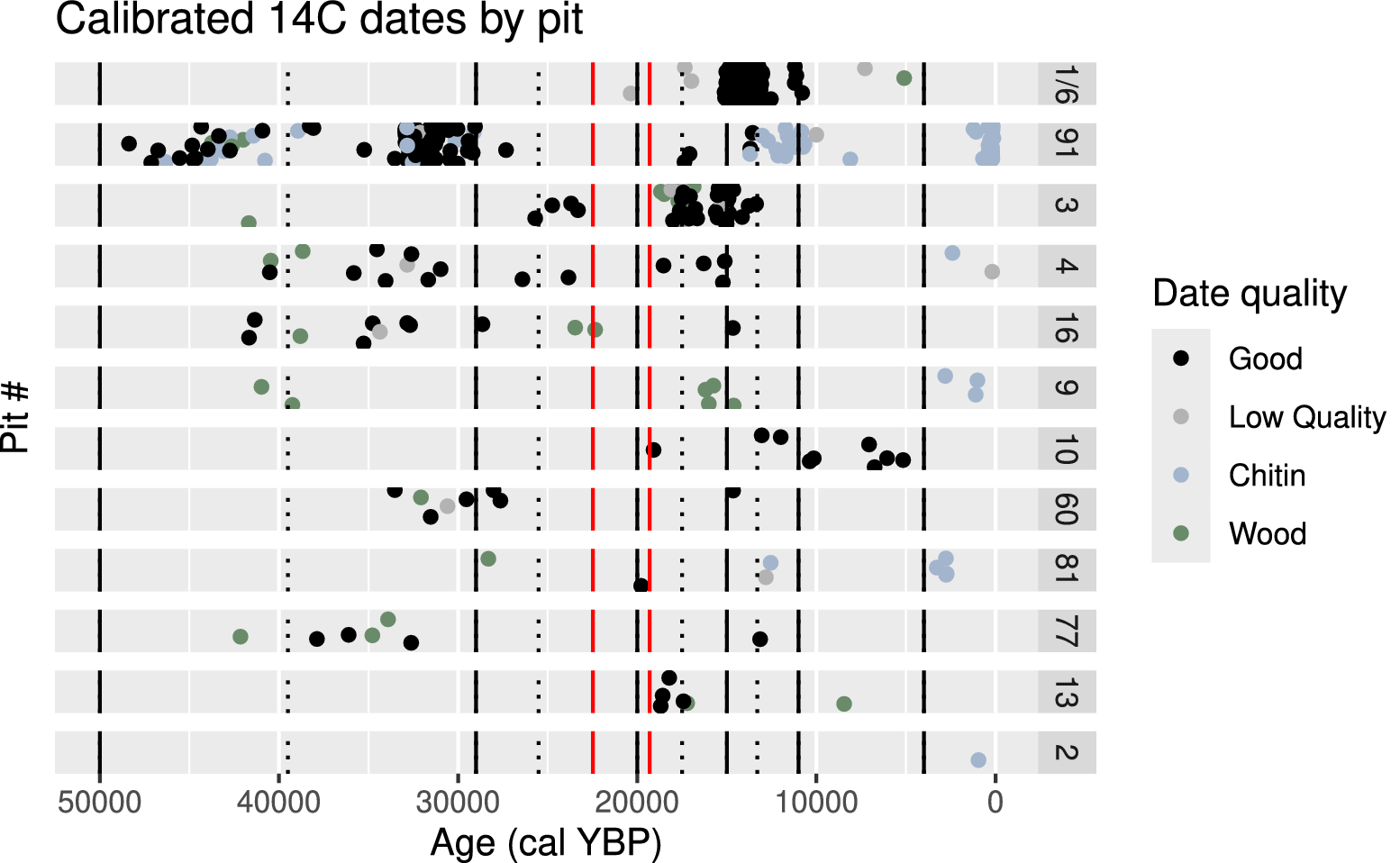
Revised Pit Age Estimates. A list of radiocarbon dates was assembled from the compilation by Fuller et al. (Reference Fuller, Harris, Farrell, Takeuchi, Southon and Harris2015) and from the lists published in five subsequent studies (Holden and Southon Reference Holden and Southon2016; Holden et al. Reference Holden, Southon, Will, Kirby, Aalbu and Markey2017; Fuller et al. Reference Fuller, Southon, Fahrni, Farrell, Takeuchi, Nehlich, Guiry, Richards, Lindsey and Harris2020; Fox et al. Reference Fox, Southon, Howard, Takeuchi, Potze, Farrell, Lindsey and Blois2023; O’Keefe et al. Reference O’Keefe, Dunn, Weitzel, Waters, Martinez, Binder and Southon2023), provided in Supplementary Table B. After omitting the single-sided dates and two ages from Ward et al. (Reference Ward, Harris, Cerling, Wiedenhoeft, Lott, Dearing, Coltrain and Ehleringer2005) that were older than the maximum range of the IntCal20 calibration curve, we calibrated the remaining dates in OxCal 4.4 (Bronk Ramsey Reference Bronk Ramsey2001) using R package oxcAAR (Hinz et al. Reference Hinz, Schmid, Knitter and Tietze2021) based on the IntCal20 calibration curve (Reimer et al. Reference Reimer, Austin, Bard, Bayliss, Blackwell, Ramsey and Butzin2020). These dates are depicted in Figure 1, sorted by pit. All dates originally published as Pit 61, 67, or 61/67 have been combined into Pit 61/67; the radiocarbon date distributions for these three categories are identical.
Distribution of published Rancho La Brea (RLB) radiocarbon ages by pit. Only dates in black were used to generate the bootstrapped time series used in the subsequent analysis; dates in gray, blue, and green were excluded (see main text for reasons). Vertical lines indicate climate bins used in this analysis; solid lines are the primary boundaries, dotted lines are the subdivided bins. Red vertical lines indicate the last glacial maximum (LGM) depositional hiatus postulated by Fuller et al. (Reference Fuller, Fahrni, Harris, Farrell, Coltrain, Gerhart, Ward, Taylor and Southon2014).

For the purposes of estimating pit age distributions, we omitted dates with reliability rated below 2 by Fuller et al. (Reference Fuller, Harris, Farrell, Takeuchi, Southon and Harris2015), dates on the >30 kDa fraction from Fuller et al. (Reference Fuller, Fahrni, Harris, Farrell, Coltrain, Gerhart, Ward, Taylor and Southon2014), and dates from pits for which we have no measured specimens. Vertebrates are the focus of this study, so we also chose to omit dates from plant (cellulose) and insect (chitin) material and use only dates from vertebrate material (bone and bone collagen). The chitin ages are younger and wider ranging than those from associated bone, which Holden et al. (Reference Holden, Southon, Will, Kirby, Aalbu and Markey2017) suggests may reflect differences in the taphonomic processes operating on insects and large vertebrates: small organisms may become entrapped in asphalt pools too shallow to immobilize larger ones. Additionally, decomposers may lay eggs in vertebrate remains that resurface long after their death due to the churning of the asphalt. The wood and wood charcoal ages are less obviously different from the bone ages, but in some pits, the wood dates significantly expand the time range of the pit, and taphonomic differences between wood and other remains are known to produce systematic offsets (the “old-wood problem”; Schiffer Reference Schiffer1986).
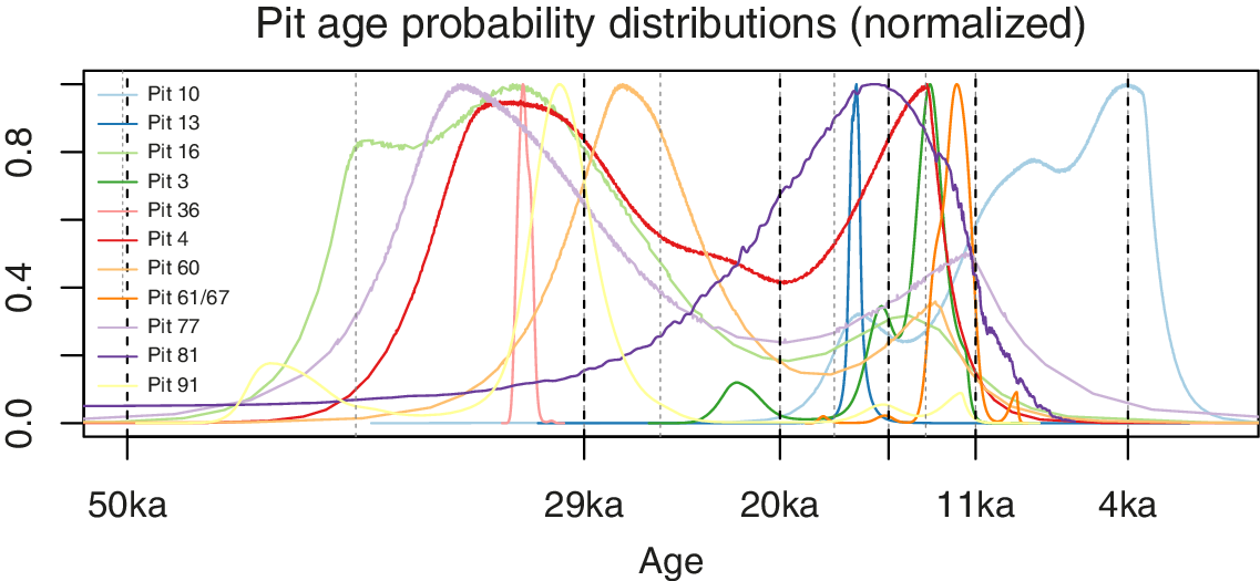
After filtering out the categories noted, we were left with 339 14C dates usable for our analysis (black dots in Fig. 1); pits 2 and 9 were omitted, having no 14C ages on vertebrate material. These dates were used to estimate an age distribution for each pit using OxCal 4.4 (Bronk Ramsey Reference Bronk Ramsey2001) with custom scripts (see Supplementary Appendix) and the R package oxcAAR (Hinz et al. Reference Hinz, Schmid, Knitter and Tietze2021). The age distributions were calculated as Bayesian kernel density estimates (KDEs) of all the calibrated dates from that pit, following the advice of Carleton and Groucutt (Reference Carleton and Groucutt2021). For pits 36 and 81, each with only a single date available, the posterior age distribution of that date was used instead. These age distributions are plotted together (normalized) in Figure 2 and separately without normalization in Supplementary Figure A. The pit KDEs were used as the basis for estimating the age distribution of the specimens, as detailed in the “Age Resampling and Time-Series Computation” section.
All pit age probability distributions based on dates in Fig. 1. Distributions have been normalized to a maximum value of 1 and overlaid to illustrate timing. Heavier vertical dashed lines correspond to time boundaries between the five main climate bins; lighter ones correspond to boundaries between the nine subdivided climate bins.
Paleoclimate Reconstruction
In all our previous studies, we based our reconstruction of RLB paleoclimate on those that were available at the time (Heusser Reference Heusser1998; Coltrain et al. Reference Coltrain, Harris, Cerling, Ehleringer, Dearing, Ward and Allen2004; Bochenski and Campbell Reference Bochenski and Campbell2006). For this study, we have instead constructed a local climate timeline based on a combination of recent papers, and we used this to designate transition points between climate intervals. A number of late Pleistocene climate estimates have been published for Southern California, Lake Elsinore, and RLB, based on a variety of proxies (Heusser Reference Heusser, Kennett, Baldauf and Lyle1995, Reference Heusser1998; Heusser and Sirocko Reference Heusser and Sirocko1997; Ward et al. Reference Ward, Harris, Cerling, Wiedenhoeft, Lott, Dearing, Coltrain and Ehleringer2005; Kirby et al. Reference Kirby, Feakins, Bonuso, Fantozzi and Hiner2013, Reference Kirby, Heusser, Scholz, Ramezan, Anderson, Markle and Rhodes2018; Fuller et al. Reference Fuller, Fahrni, Harris, Farrell, Coltrain, Gerhart, Ward, Taylor and Southon2014; Heusser et al. Reference Heusser, Kirby and Nichols2015; Holden et al. Reference Holden, Southon, Will, Kirby, Aalbu and Markey2017; Fox et al. Reference Fox, Southon, Howard, Takeuchi, Potze, Farrell, Lindsey and Blois2023; O’Keefe et al. Reference O’Keefe, Dunn, Weitzel, Waters, Martinez, Binder and Southon2023). Here, we have used these to estimate major climate phases at RLB in order to choose breaks between time bins for our time-series analysis that best correspond to the intervals of environmental change. The break points given in these publications are shown in Figure 3.
Timeline of regional climate events and local climate chronology based on Heusser Reference Heusser, Kennett, Baldauf and Lyle1995, Reference Heusser1998; Heusser and Sirocko Reference Heusser and Sirocko1997; Ward et al. Reference Ward, Harris, Cerling, Wiedenhoeft, Lott, Dearing, Coltrain and Ehleringer2005; Kirby et al. Reference Kirby, Feakins, Bonuso, Fantozzi and Hiner2013, Reference Kirby, Patterson, Lachniet, Noblet, Anderson, Nichols and Avila2019; Fuller et al. Reference Fuller, Fahrni, Harris, Farrell, Coltrain, Gerhart, Ward, Taylor and Southon2014; Heusser et al. Reference Heusser, Kirby and Nichols2015; Holden et al. Reference Holden, Southon, Will, Kirby, Aalbu and Markey2017; Feakins et al. Reference Feakins, Wu, Ponton and Tierney2019; Fox et al. Reference Fox, Southon, Howard, Takeuchi, Potze, Farrell, Lindsey and Blois2023; O’Keefe et al. Reference O’Keefe, Dunn, Weitzel, Waters, Martinez, Binder and Southon2023. The numeric boundary values used to generate this figure are given in Supplementary Table C. DG, Deglacial; Hol., Holocene; HS-1, Heinrich Stadial 1; LGM, last glacial maximum; MIS, Marine Isotope Stage; RLB, Rancho La Brea; Tr., Transitional.
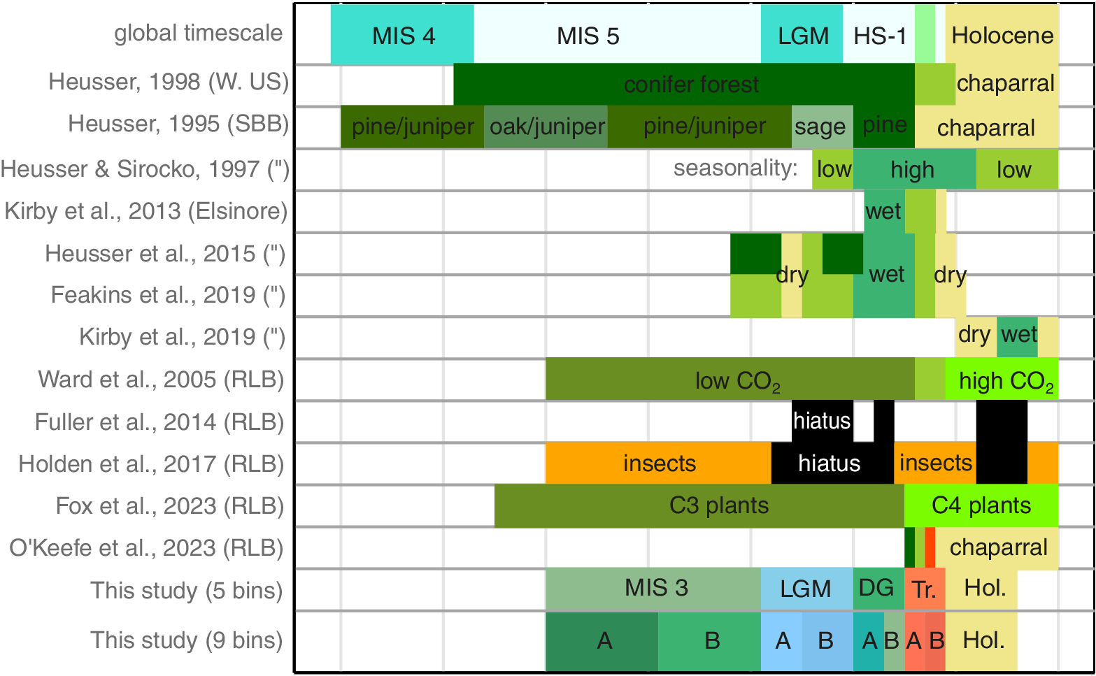
The multi-proxy climate reconstruction of the interval from 15.6 ka to 10 ka by O’Keefe et al. (Reference O’Keefe, Dunn, Weitzel, Waters, Martinez, Binder and Southon2023) was generated using break-point analysis of multiple climate time series to infer local climate changes. We have not attempted such a rigorous reconstruction here, although we suspect that the data available may be sufficient for such an analysis. Instead, we used the break points described in the text of the original publications to choose our climate intervals by eye, weighting proxies by their proximity to the Los Angeles Basin. After testing revealed that our original five climate bins produced time series that were too short for a model testing approach, as discussed in the “Results” section, we also defined a set of nine bins. The break points transcribed from the literature and our resulting climate intervals are given in Supplementary Table C and depicted in the bottom two lines of Figure 3. The vertical dashed lines in Figures 1 and 3 give the boundaries between the main five climate intervals.
Our interval boundaries were chosen to capture the consensus in the regional climate reconstruction literature. Interval 1 (“MIS 3,” 50–29 ka) corresponds to the cooling from the LIG into the LGM; lacking any distinct regional climatic break points, we simply divided it in half at 39.5 ka. Interval 2 (“LGM,” 29–20 ka) goes up to the end of the cold and dry period according to Heusser et al. (Reference Heusser, Kirby and Nichols2015). We split it in half at 25.5 ka, such that LGM-A contains the 27.5–25.5 ka drought noted from the Lake Elsinore cores (Heusser et al. Reference Heusser, Kirby and Nichols2015; Feakins et al. Reference Feakins, Wu, Ponton and Tierney2019) and LGM-B contains most of the 22.5–19.3 ka RLB depositional hiatus (18–16.5 uncalibrated 14C ka BP) (Fuller et al. Reference Fuller, Fahrni, Harris, Farrell, Coltrain, Gerhart, Ward, Taylor and Southon2014). Interval 3 (“Deglacial”) covers the cold and wet period from 20 to 15 ka; the midpoint split at 17.5 ka is again simply for convenience. Interval 4 (“Transitional,” 15–11 ka) corresponds to the interval analyzed in detail by O’Keefe et al. (Reference O’Keefe, Dunn, Weitzel, Waters, Martinez, Binder and Southon2023), with the first half (15–13.3 ka) approximately coinciding with the warm Bølling-Allerød interstadial, and the second (13.3–11 ka) to the wildfire interval of O’Keefe et al. (Reference O’Keefe, Dunn, Weitzel, Waters, Martinez, Binder and Southon2023) and the Younger Dryas. The remainder of the time (11–4 ka) is a single Holocene interval, as there were not enough vertebrate dates available to justify splitting it.
Age Resampling and Time-Series Computation
Due to the severely nonparametric distribution of ages in each pit, as discussed earlier, we used a bootstrapping procedure to estimate the age distributions of the measurements. This procedure makes the following assumptions: (1) complete time averaging within pits; (2) unbiased sampling of specimens for dating; (3) reasonably complete sampling of each pit; and (4) a single age distribution that applies equally to all taxa.
For each specimen (individual measured bone) in the database, an age was drawn at random from the computed probability distribution for its pit and assigned to that specimen; this procedure was replicated 1000 times. This bootstrapped dataset was used to generate averaged time series of each measurement on each element, as follows: For each time bin in the time series, the average age was computed as the grand mean of assigned specimen ages in that time bin among all bootstrap replicates, and the average sample size as the mean number of specimens in the time bin among all replicates. Then, again for each time bin in the time series, the average for each measurement taken on that element was computed as the grand mean of the values of that measurement for each replicate, and the average variance was computed as the mean of the variances for each replicate. These time series were generated for all direct measurements as well as for the first and second PCs of the variation for each specimen in each species. To assess the possible bias toward stasis introduced by this averaging procedure, 250 individual replicate time series for each element were also subjected to model fitting (see next section).
Time-Series Model Fitting
The bootstrapped and averaged time series generated by the procedure above were analyzed using the R package paleoTS to compare fit with different evolutionary models. The time-series models compared were those described in paleoTS as URW (unbiased random walk), GRW (directional random walk), Stasis, StrictStasis, and Punc-1 (a single shift). GRW models each consecutive step in the time series by drawing a change in trait value (Δx) from a normal distribution, the mean and variance of which are parameters of the model. URW is the same, but the mean of the Δx distribution is fixed at zero. Stasis draws the new value of x, rather than Δx, from a normal distribution with modeled mean and variance, and StrictStasis is the same but with the variance of the trait distribution fixed at zero. The Punc model is the only complex (changing) model used in this study; it has two segments of Stasis, with different values of mean and variance, plus a single time point at which both are allowed to shift. For precise definitions of the models, see Hunt et al. (Reference Hunt2007, Reference Hunt, Hopkins and Lidgard2015) or the paleoTS documentation (Hunt Reference Hunt2022). The models were compared based on the corrected Akaike information criterion (AICc) weights; the AICc is an estimate of the quality of the model fit that accounts for the number of model parameters, and Akaike weights allow comparison by transforming the AICc values into a vector of proportional support for all tested models. The parameters for the four models were also compared in order to estimate the speed of evolutionary change.
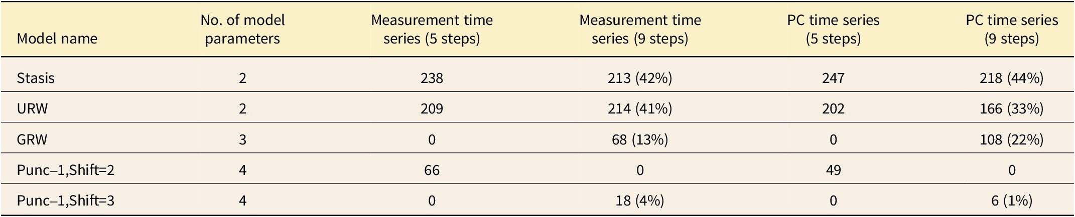
Testing Time Series Length. To capture sensitivity to time-series length, the model fitting procedure was repeated using two different sets of time bins. As described in the “Paleoclimate Reconstruction” section, the first set has five bins and the other nine. The two sets of time bins are depicted in the vertical lines in Figure 1 and given in Supplemental Table C. For short time series, the number of time points strongly biases the choice of models. The models used vary from one to four parameters, and when the time series has only five points, the AICc comparison strongly favors models with the fewest parameters. On the other hand, dividing an empirically defined time series arbitrarily into smaller intervals tends to make the model selection procedure favor an unbiased random walk (URW). The time-series model fitting results, as summarized in Table 3, reflect this: 90% of the shorter five-step time series were best fit by the simplest model (StrictStasis). This is an unavoidable limitation of the time-series model fitting method.
Summary statistics for paleoTS time-series model fits on measurement and principal component (PC) time series. GRW, generalized random walk; URW, undirected random walk; Punc-1, punctuated equilibrium with 1 shift. Changes were detected in largely the same set of bones in both five-interval and nine-interval time series, but the shorter time series favored stasis/URW over directional and punctuated over gradual models.

Omitting the StrictStasis model and fitting only models with two or more parameters transfers the same bias to the two-parameter models (Stasis and URW), but also detects more of the directional trends that appear to the eye. When we split all intervals except the Holocene in half, creating a nine-step time series, this dropped to 70%. Using even smaller time bins starts to create problems with the smaller datasets: if there are too few specimens, the bootstrap resampling procedure creates so much collinearity in the resampled time series that the results are impossible to interpret. To accommodate this effect, we have restricted our time-series model fits to the nine-step time series, because the shorter time series effectively cannot be fit using this method. We have also omitted the StrictStasis model and compared only GRW, URW, Stasis, and Punc-1. The results and interpretations given later reflect these decisions.
Testing the Bootstrapping and Averaging Procedure. Comparison of the first 250 bootstrapped time series for each measurement to the averaged time series reveals that the averaging procedure makes the resulting time series less likely to be modeled as stasis. To give a single illustrative example of this effect, although 88% of 250 individual time series of S. fatalis humerus length were best modeled as either URW or Stasis and only 12% as GRW, the GRW model is strongly favored for the averaged time series (Akaike weight 0.58, compared with 0.39 for URW and 0.3 for Stasis) (see Supplementary Fig. D). The same effect holds for the rest of the dataset: the weights of the two-parameter URW and Stasis models are greater for the individual bootstrap replicates than in the averaged time series, while the reverse is true for the three-parameter GRW model (an overall comparison of individual vs. averaged Akaike weights for all nine-step time series is given in Supplementary Fig. E). We interpret this to mean that the averaging procedure successfully filters out some of the noise introduced by the bootstrapping procedure and makes it easier to recover the true signal. We also surmise that the noise introduced by the previous age estimation method, similarly, may have artificially increased the prevalence of stasis as the best-supported model in our original studies.
Results
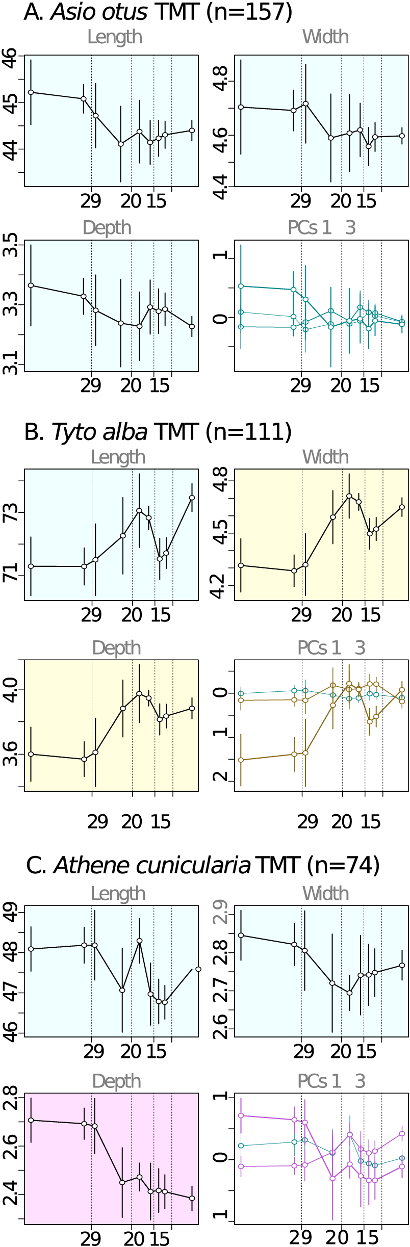
The results of the time-series model fits are summarized in Table 3. Three example time series are plotted in Figure 4, as discussed here; to emphasize the diversity of morphological responses among ecologically similar groups in our sample, all three examples are TMTs of extant owl species. Due to the size of the dataset, the complete results are not printed here; instead, all time series are plotted by species in the Supplementary Appendix, and all model weights and model fit parameters for those time series are given in Supplementary Table E.
Example measurement and principal component (PC) time series reconstructed from Rancho La Brea (RLB) fossil tarsometatarsi (TMTs) of three extant owls. Colors indicate best-fit time-series model: pink, GRW (directional random walk); red, Punc (a single shift); yellow, URW (unbiased random walk); blue, Stasis. All PCs are plotted together, with wider lines indicating higher PCs, and line colors similarly indicating best fit time-series models. A, Asio otus TMT: all time series are best fit by a Stasis model, including all PCs. B, Tyto alba TMT: most time series are best fit by a URW (random walk) model. C, Athene cunicularia TMT: most time series are best fit by a GRW (directional evolution) model.

The majority of nine-step time series were best fit by either a stasis or a random walk (URW) model (83% of measurements and 92% of PCs); and for 23 of the 30 species, all time series are best fit by Stasis and/or URW. As described earlier, this is partially the effect of a preference for the simplest available model for short time series. However, it is visually apparent from the time-series plots that the size and shape of most of the bones examined here genuinely do not appear to change significantly over the Pleistocene/Holocene transition. The difference between undirected random walk (URW) and stasis (Stasis) is not always evident, and in most cases (29 of 57 bones), the best models for the various measurements and PCs of a single bone are all either Stasis or URW. In a few cases, stasis is clearly a better model for all the time series; for example, Asio otus (Fig. 4A). Much more common is a combination of Stasis and URW, as in Tyto alba (Fig. 4B), in which some time series have significant departures from the mean or even appear to display nonlinear trends; however, detailed interpretation is difficult at this temporal resolution.
The overall evolutionary variance of a trait among time bins is modeled by the “omega” parameter of the Stasis model fit, regardless of the relative weights of the models. Normalizing this parameter by dividing by the mean variance in the last three time intervals, which have relatively narrowly constrained time distributions (see Fig. 2), then taking its square root, we arrive at a value expressed in centimeters that can be used as a measure of the variability of the trait, assuming a static mean through time, which we will refer to as “evolutionary variance.” The magnitude of directional trend is reflected in the mstep parameter of the GRW model fit; for ease of discussion, we have divided the time-agnostic values of the model parameters by the average time-step size in order to convert them to millimeters per million years (mm/Myr).
The evolutionary variance of most of our traits is zero: that is, the populations in different time bins are similar enough that no variance is necessary to model them (corresponding to the StrictStasis model). This is the case for 51% of the nine-step time series and 65% of the five-step time series, all of which are best modeled as Stasis or URW. Nonzero evolutionary variances are more common in the nine-step time series, which again supports the interpretation that the longer intervals in the five-step series produce larger within-interval variances, impeding our ability to detect change over time.
Directional evolution (GRW) was the favored model for at least one dimension or PC for 28 bones in 13 species. In all three of the bones containing time series for which a stepwise (Punc-1) model was favored, GRW was also favored for other time series. We conclude that the temporal resolution of our data (nine steps) is evidently insufficient to discriminate between stepwise and gradual change. Among the time series best modeled by a directional trend (either GRW or Punc-1), the values of the evolutionary variance parameter are significantly greater than for those for which nondirectional models (URW or Stasis) were favored, and among directional time series, higher evolutionary variance is associated with greater weight of the GRW model. Similarly, the magnitudes of the trend parameter in the GRW model (GRW.mstep) are significantly greater among directional time series than among those best fit by the nondirectional models (p = 0.0005). However, the magnitude of the trend parameter was not correlated with the model weight; that is, for a time series displaying a directional evolutionary trend, the size of the trend and its strength were unrelated.
The majority (two-thirds) of the directional trends are toward smaller and/or more gracile forms (Supplementary Table D); trends toward smaller forms also accounted for more variance in the data than those toward larger forms. Figure 4C (Athene cunicularia) is a good example of this tendency, as are some elements in Equus occidentalis and Gymnogyps amplus and calcanea of Camelops hesternus, as discussed later. However, several exceptions to the overall trend are noted. The most notable of these is the saber-toothed cat Smilodon fatalis, in which all the measured postcranial bones increase in size (see Supplementary Appendix A and Supplementary Table D) and are all best fit by directional models with evolutionary rates between 0.1 and 1.3 mm/Myr. This is consistent with other studies on crania in S. fatalis (Meachen et al. Reference Meachen, O’Keefe and Sadler2014; Goswami et al. Reference Goswami, Binder, Meachen and O’Keefe2015) but contradicts the study we previously published using the same dataset (Madan et al. Reference Madan, Prothero and Sutyagina2011). Among the other time series with increasing size, many are either low-variance PCs of otherwise static or shrinking bones (e.g., Aenocyon, Equus, Panthera, Gymnogyps crania) or based on especially small sample numbers (e.g., Lynx), although astragali of Paramylodon and TMTs of a few birds also increase in size and robustness.
Discussion
Stasis and Climate Change
Prevalence of Stasis
The majority of our results were consistent with those of our previous studies, despite the major methodological difference: the majority of bones in the majority of species remain static in size and shape through the onset and departure of the LGM. Comparing our results with the 9–14% directional evolution benchmark from Hunt et al. (Reference Hunt, Hopkins and Lidgard2015) and Voje (Reference Voje2016), we find directional evolution in 13% of nine-step time series of direct measurements and 22% of PCs of variation. Directional evolution in this dataset thus appears to be slightly more common than the average for all morphological time series, although many of the directional changes occurred in noisy low-variance PCs.
There is no indication of larger body size or more robust limb proportions at the LGM, as might be predicted by Bergmann’s rule and Allen’s rule. If Bergmann’s rule was driving local evolution or range shift, we would expect steady or increasing body size and robustness going from the MIS-3 intervals (1–2) into the LGM intervals (3–4), followed by a decrease over the Deglacial and Transitional intervals (5–8). This is not evident in any of the time series. Instead, size and robustness seem to reflect other factors, which may be more easily determined upon individual consideration of each species’ particular ecological role. Although a complete evaluation of each species is beyond the scope of this paper, Gymnogyps californianus ssp. amplus (G. amplus) and Equus occidentalis both furnish useful examples. Both these species display a robust non-static trend in a large sample size, which allows more detailed interpretation.
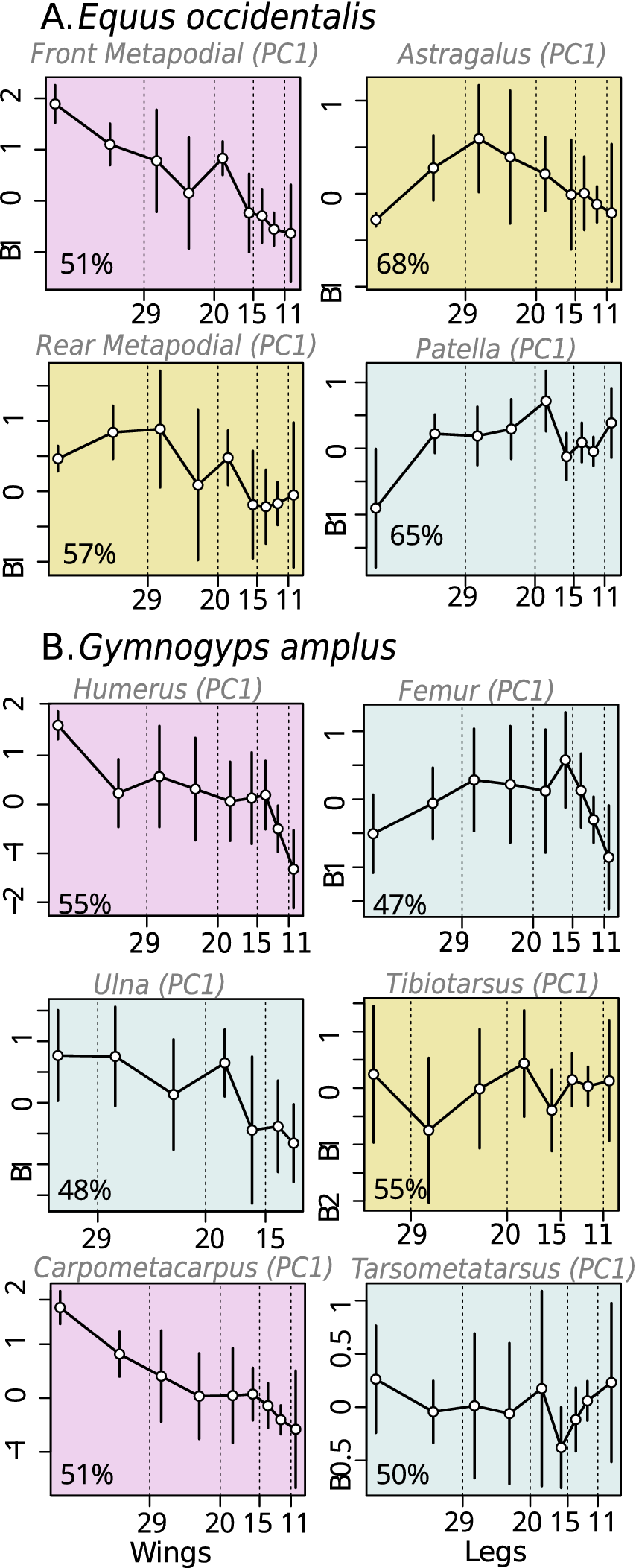
All PC 1 time series from these two species are given in Figure 5. In Equus, the third metacarpals (forelimb cannon bones) have an obvious linear trend, continually shorter and thinner (−0.2 mm/Myr), interrupted by an upward tick in the first Deglacial interval. This is the only element in Equus with such a strong trend: the astragalus becomes somewhat shorter and thicker, the third metatarsal (hindlimb cannon bone) somewhat more gracile, and the patella is static. Notably, the calcanea of Camelops hesternus also display a strong trend toward smaller size beginning in the first Deglacial interval (−2.1 mm/Myr). Although this raises the interesting possibility that these two ecologically similar cohabiting species may have been subject to similar pressures during the Pleistocene/Holocene transition, unfortunately neither calcanea of E. occidentalis nor cannon bones of C. hesternus were measured, so no further comparison of the two is possible.
Principal component 1 (PC 1) time-series plots for (A) all four measured skeletal elements of Equus occidentalis and (B) forelimbs and hindlimbs of Gymnogyps amplus (G. californianus), with colors as in Fig. 4. Percentage of variation is given in gray at top right of each plot; all PCs have been rotated so that positive = larger. The third metacarpal (cannon bone) of E. occidentalis decreases continually along PC 1, but the other three have no directional trend. The three wing bones of G. amplus also each decrease along the respective PC 1, but the leg bones have no directional trend. Colors are as in Fig. 4.

The results for Gymnogyps are more straightforward to interpret: the two bones with clear downward trends in all dimensions are both from the wing, the carpometacarpus (PC1: −0.2 mm/Myr) and humerus (PC1: −0.2 mm/Myr), and the ulna appears to follow the same trajectory, although the sample is too small to discriminate models. All the lower limb bones (femur, tibiotarsus, and TMT) are static. The skulls have a mixture of different trajectories reflecting their variety of functions; cranial height increases and foramen magnum shrinks, but the majority of skull measurements display no directional change. Evidently wing size in Gymnogyps and forelimb length in Equus both decreased continually through the transitions into and out of the LGM temperature minimum and thus could not have been responding directly to temperature. These two examples are illustrative of the general lack of apparent temperature correlation among the species studied here, whether static or variable.
Ephemeral Changes
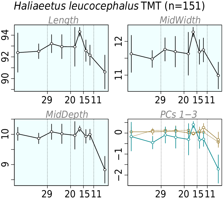
Two particular intervals have anomalous means in enough time series that they merit individual attention. These phenomena are both visible in the time series for Haliaeetus leucocephalus (Fig. 6). First, many species and anatomical elements have a visible difference between the Holocene individuals (11–4 ka) and the rest of the Pleistocene. This shift occurs in the last time bin and is therefore not captured by the time-series analysis. However, this observation is consistent with the conclusions of O’Keefe et al. (Reference O’Keefe, Dunn, Weitzel, Waters, Martinez, Binder and Southon2023) regarding the ecological regime shift at the end of the Pleistocene. Interestingly, this appears to apply mainly to extant species. An anomalous interval also often appears somewhere between 20 and 13.3 ka. In Haliaeetus, this appears in the Deglacial B interval (17.5–15 ka), but it occurs one interval earlier or later in some other species, and may be from one to three intervals long. The direction of the change is not consistent. This timing corresponds to the wettest climatic interval in the regional climate record. Further detailed exploration of the validity and possible causes of this potentially interesting phenomenon will not be undertaken in this study.
Time series of measurements and principal components (PCs) for Haliaeetus leucocephalus tarsometatarsi (TMT), with colors as in Fig. 4. The population means are generally static throughout, with two points of apparently ephemeral change standing out: the 18–15 ka population is longer and broader than the mean, and the 11–4 ka point is smaller in all dimensions. Colors are as in Fig. 4.

Methodological Comparison
Assigning all individuals in a pit to the mean age of the pit can, as Fuller et al. (Reference Fuller, Harris, Farrell, Takeuchi, Southon and Harris2015: p. 165) put it, “mix samples from very different climate regimes and potentially blur or even obliterate important temporal changes in morphological or isotopic data” by adding a random error to each individual’s actual age. This kind of time error would tend to obscure real differences between time bins without introducing any directional bias and therefore would decrease the chance of any statistical time-series method detecting directional evolution. The time-series modeling approach also means that the results returned by this analysis, as well as its predecessors, are biased in favor of low parameter number models, especially for short time series or small samples, which would also disproportionately favor stasis or random walk models. It is encouraging, therefore, that this method detected non-stasis (GRW/Punc) in a number of cases that were not previously noticed. In particular, the new approach is validated by its ability to detect the same trend toward larger size in S. fatalis postcranials that appeared in the mandibles (Meachen et al. Reference Meachen, O’Keefe and Sadler2014) and crania (Goswami et al. Reference Goswami, Binder, Meachen and O’Keefe2015), whereas our previous paper using these data failed to detect it (Madan et al. Reference Madan, Prothero and Sutyagina2011).
A similar comparison can be made for Aenocyon dirus: our results here, measured on postcranials, largely echo those of Brannick et al. (Reference Brannick, Meachen, O’Keefe and Harris2015) on the mandibles using geometric morphometrics. Many of the A. dirus measurements in our Deglacial interval are distinctly smaller; this corresponds to their observations of mandibles from Pit 13, which contributes a significant proportion of the individuals in this interval. The mean sizes of postcranials also rebound to their previous averages in the Transitional and Holocene intervals, like their mandibles. We note, though, that the specimens assigned to the Transitional intervals in our study are not larger than the overall static average, unlike the Pit 61/67 individuals of Brannick et al. (Reference Brannick, Meachen, O’Keefe and Harris2015). Perhaps the overlap with Pit 3 in our study has obscured this signal, or perhaps the size increase during the Transitional interval applies only to the mandible.
With this in mind, we must revise our previous conclusions on the following taxa: A. cunicularia, Buteo swainsoni, C. hesternus, Circus hudsonius, Corvus corax, E. occidentalis, Gymnogyps amplus, Paramylodon harlani, and S. fatalis. In these 10 taxa, contra our original publications, the reanalysis indicates that at least some significant directional change did take place in the size/shape of at least one and often several bones. In the other taxa for which some directional change was detected (A. dirus, Caracara prelutosa, Lynx rufus, Panthera atrox, and Sturnella neglecta), the evidence is equivocal, either because the sample size was especially small or because directional trends appeared only in low-variance PCs.
Depositional Hiatus
On the basis of this chronology revision, we can confirm the depositional hiatus noted by Fuller et al. (Reference Fuller, Fahrni, Harris, Farrell, Coltrain, Gerhart, Ward, Taylor and Southon2014). The interval between 18.5 and 16 uncalibrated 14C ka BP, which corresponds to approximately 22.4 to 19.3 calendar ka BP, has not been filled by results from subsequent papers. In our analysis, this gap corresponds to the end of the LGM bin and the beginning of the Deglacial bin. The hiatus interval is marked in red on Figure 2, where it can be seen that only three dates fall within it. Of these three, one has unusually large errors, ±3250 years (sample QC405b of Marcus and Berger [Reference Marcus, Berger, Martin and Klein1984], Pit 81); one is unreliable due to being from the >30 kDa fraction (sample UCIAMS91653 of Fuller et al. [Reference Fuller, Fahrni, Harris, Farrell, Coltrain, Gerhart, Ward, Taylor and Southon2014], Pit 61/67); and the third is from a wood sample (sample 427R of Marcus and Berger [Reference Marcus, Berger, Martin and Klein1984], Pit 16), which may be unreliable on account of the long environmental residence time of dead wood (Schiffer Reference Schiffer1986). For discussion of possible reasons for this hiatus, see Fuller et al. (Reference Fuller, Fahrni, Harris, Farrell, Coltrain, Gerhart, Ward, Taylor and Southon2014).
Conclusions
Previous studies of the mammals and birds of RLB by our research group tended to document stasis in most of the morphological variables through most of the late Pleistocene in all 9 mammals and 19 birds that were studied. This was already clear from analysis of variance studies of all the samples (in taxa that were abundant enough for parametric tests), where no pit stood out from the pooled mean of all pits. In particular, there was no evidence of larger individuals with more robust limbs during the peak glacial interval, as would be predicted from Bergmann’s rule or Allen’s rule, so there was no simple response to climate change in those studies. With newer radiocarbon dates and better estimates of the ages of the specimens, we still do not see an obvious response to the colder conditions of the last glacial interval, but there are indications of a response to the climate change at the glacial/interglacial transition, at the same time that most of the megamammals and many of the birds went extinct. In fact, the patterns are now more complex: stasis or at least no evidence of directional change in the vast majority of the taxa and anatomical elements sampled, but some directional change in a few taxa, none of it correlated in a straightforward fashion with the climate changes in this time interval. Thus, it appears that the birds and mammals of RLB did not respond straightforwardly to climate by becoming smaller as the climate warmed, but some measurements do appear to have responded to the variety of ecological changes during the Pleistocene/Holocene transition.
Several possible follow-up studies are suggested. First, the resampling method in this paper could help to illuminate the effect of temporal uncertainty on time-series modeling results. By generating simulated time series with known evolutionary modes and simulated age uncertainty distributions, resampling them, and assessing the fidelity of the resulting model fits, one could parameterize the recoverability of different evolutionary patterns as a function of time averaging. Second, although we have reevaluated the major claims in the preceding paper series, this review has not fully examined the extensive amount of data presented herein. For 10 of these species there are multiple anatomical elements present in our dataset, which offers an opportunity to examine whether changes in different body parts are coordinated. For example, most of Gymnogyps amplus remains unchanged through the interval, but the cranium, carpometacarpus, and humerus decrease in size. In particular, examining our outlier Smilodon fatalis in detail and in conjunction with other recent studies of dietary isotopes, morphology, and developmental integration in Smilodon (Coltrain et al. Reference Coltrain, Harris, Cerling, Ehleringer, Dearing, Ward and Allen2004; Meachen et al. Reference Meachen, O’Keefe and Sadler2014; Goswami et al. Reference Goswami, Binder, Meachen and O’Keefe2015; Fuller et al. Reference Fuller, Southon, Fahrni, Farrell, Takeuchi, Nehlich, Guiry, Richards, Lindsey and Harris2020) might illuminate the relationship between environment, morphology, and extinction. Comparing the trajectories of species with respect to their shared ecological traits might cast light on the specific environmental pressures affecting the RLB vertebrate community during the Pleistocene/Holocene transition.
Competing Interests
The authors declare no competing interests.
Data Availability Statement
Supplementary files are available at github.com/vjpsyverson/RLB/size_glacial/2023Paleobio/Final/Supplementary. All other data and code for this paper are available at github.com/vjpsyverson/RLB/size_glacial/2023Paleobio. Time series of measurements will also be uploaded to the Phenotypic Evolution Time Series database (pets.nhm.uio.no/).
Acknowledgments
Our numerous coauthors on the preceding studies in this series, listed in Table 1, collected the data. We thank the reviewers, particularly G. Hunt, for their extensive and insightful comments on the statistical methods, and the editors of the special issue for the invitation to contribute.


 Open access