


1. Introduction
Sloshing is a violent movement of a liquid within a container. It may be important to consider the interaction with support structures. When the surge and/or pitch period of the support structure is close to the first sloshing natural period, strong oscillation nonlinearities occur (see e.g. Faltinsen & Timokha Reference Faltinsen and Timokha2021).
Due to the high local and global loads associated with the impact of waves against the sidewall, sloshing flows have several implications from a practical point of view. For example, in the naval framework, knowledge of the flow characteristics that occur during the violent motion of liquids within confined spaces (Silverman & Abramson Reference Silverman and Abramson1966), is a fundamental issue for the safety of liquid natural gas carriers. Since these ships operate with different tank filling conditions, it is important to understand in depth the main features of the phenomena involved. In particular, the filling height of the tank can drastically change the regimes observed when the tank is almost completely (Rognebakke & Faltinsen Reference Rognebakke and Faltinsen2005), partially (Colagrossi et al. Reference Colagrossi, Palladino, Greco, Lugni and Faltinsen2006; Jin et al. Reference Jin, Tang, Tang, Mi, Wu, Liu and Huang2020) or barely filled (Bouscasse et al. Reference Bouscasse, Colagrossi, Colicchio and Lugni2007; Antuono et al. Reference Antuono, Bouscasse, Colagrossi and Lugni2012a, Reference Antuono, Bardazzi, Lugni and Brocchini2014). Violent free-surface flows can occur when the energy spectrum of the vessel's motion is focused in the region near the lowest natural mode of the tank. Then, large slamming loads (Faltinsen, Landrini & Greco Reference Faltinsen, Landrini and Greco2004; Lugni, Brocchini & Faltinsen Reference Lugni, Brocchini and Faltinsen2006a) may occur, with possible air entrapment (Lugni, Brocchini & Faltinsen Reference Lugni, Brocchini and Faltinsen2010a; Lugni et al. Reference Lugni, Miozzi, Brocchini and Faltinsen2010b), which also compromises the integrity of the structure (Lugni et al. Reference Lugni, Bardazzi, Faltinsen and Graziani2014). In this condition, an appropriate prediction of the impulsive loads and their duration can be useful for an adequate estimate of the fluid–structure interactions (see e.g. Marrone et al. Reference Marrone, Colagrossi, Park and Campana2017; Fang et al. Reference Fang, Ming, Wang, Meng and Zhang2022; Pilloton et al. Reference Pilloton, Bardazzi, Colagrossi and Marrone2022).
Although correct modelling of the local evolution of the flow field is crucial for the description of the fluid loads, it is also extremely important to consider the global characteristics of the flow during the tank motion. Typically, they are classified with respect to the occurring wave patterns. A first classification was given for sloshing flows in shallow water by Olsen & Johnsen (Reference Olsen and Johnsen1975). It is well known that the low filling depth condition can induce strong nonlinear effects leading to four different scenarios: (a) a standing wave; (b) a combination of standing and travelling wave systems; (c) a hydraulic jump, characterizing the propagation of breaking waves; (d) a pure travelling wave. For the latter case, the interaction of the wave train with the lateral walls of the tank can lead to the formation of ascending water jets which climb the vertical wall with consequent rundown and trapping of air bubbles (Bouscasse et al. Reference Bouscasse, Antuono, Colagrossi and Lugni2013).
In general, in sloshing flows induced by purely periodic lateral motion, the free surface moves with a period strictly related to the excitation frequency. When the latter approaches resonant conditions, superharmonic components appear, induced by the nonlinear effects. In addition to this, the identification of peculiar behaviours of nonlinear sloshing flow such as subharmonic or chaotic modes requires the analysis of several conditions that vary with filling heights, amplitudes and frequencies of the tank motion.
This approach was adopted during the first experimental campaign at CNR-INM (formerly INSEAN) in 2003. The experimental set-up of a similar campaign conducted in the 1970s by Olsen (Reference Olsen1970) was reproduced. The same tank dimensions, i.e. squared  $L\times L$ with $L=1$ m, and the same filling depth, i.e. $h/L=0.35$ close to the critical one, were considered.
According to Tadjbakhsh & Keller (Reference Tadjbakhsh and Keller1960), the sloshing dynamics at a frequency close to resonance has been shown to produce a response that changes from a ‘hard-spring’ to a ‘soft-spring’ response as the depth passes through a critical value, theoretically evaluated as  $h/L=1.07/{\rm \pi} \simeq 0.3406$ (where h is the water depth; see also Kovacic & Brennan Reference Kovacic and Brennan2011). Fultz (Reference Fultz1962) reports an experimental confirmation of these results and underlines that the frequency effect reversal appears to occur at a depth ratio of $h/L=0.88/{\rm \pi} \simeq 0.28$, somewhat less than the theoretical value. This discrepancy is related to the effect of a non-infinitesimal forcing amplitude. The difference between the value of 0.28 found by Fultz (Reference Fultz1962) and 0.34 of Kovacic & Brennan (Reference Kovacic and Brennan2011) is not crucial for the present work, while what is really relevant is that the filling depth adopted, i.e. $h=0.35L$, is sufficiently close to and above the critical depth to guarantee a clear soft-spring behaviour in the sloshing dynamics investigated. The theoretical value of critical depth has been estimated (calculated) theoretically by many authors, and the interested reader can also refer to e.g. Ockendon & Ockendon (Reference Ockendon and Ockendon1973), Waterhouse (Reference Waterhouse1994), Faltinsen et al. (Reference Faltinsen, Rognebakke, Lukovsky and Timokha2000) and Faltinsen & Timokha (Reference Faltinsen and Timokha2009). Incidentally, the hard-spring behaviour was previously studied experimentally and numerically in Antuono et al. (Reference Antuono, Bouscasse, Colagrossi and Lugni2012a) and Bouscasse et al. (Reference Bouscasse, Antuono, Colagrossi and Lugni2013) with filling depths ranging from 0.03 to 0.125. There, simulations were performed using a smoothed particle hydrodynamics (SPH) model as in the present work.
As in Olsen (Reference Olsen1970), in order to limit the three-dimensional (3-D) effects, the thickness of the tank was set equal to  $0.1 L$. In Olsen (Reference Olsen1970), the surface elevation was measured with a wire probe positioned 5 cm from one of the vertical sides of the tank. In addition to this, another three wire probes were used in the CNR-INM campaign. In particular, a wire probe was positioned 5 cm from the other vertical side of the tank to check for any non-symmetrical flow behaviour.
During each test, a sinusoidal movement with prescribed amplitude and frequency was imposed on the tank. A range of different frequencies and amplitudes was investigated through analysis of the surface elevation, measured locally by the wire probes and globally by video recording. Following the experimental procedure detailed in Olsen (Reference Olsen1970), 300 s of motion were recorded to attain a stable regime condition. In Colagrossi (Reference Colagrossi2005) and Colagrossi et al. (Reference Colagrossi, Lugni, Greco and Faltinsen2004), the experimental matrix test was also studied numerically through a SPH model. The maxima of the numerical time signals were identified and compared with the experimental data of Olsen (Reference Olsen1970) and with the theoretical results predicted by the multi-modal approach of Faltinsen & Timokha (Reference Faltinsen and Timokha2001). In particular, three amplitudes of oscillation  $A=0.025L$, $A=0.050L$, $A=0.100L$ were analysed and the data were compared against the numerical outcomes, showing a good agreement with the experimental data.
Following the same path, in the present work a more accurate analysis of the surface elevation is carried out for  $A=0.01L$ and $A= 0.03L$, by considering the time signals of different wave probes near the vertical walls of the tank. In addition to the values of the maxima taken into account by Olsen (Reference Olsen1970), the full time history of the surface elevation is investigated, identifying the regimes attained by the flow motion.
Similarly to Durante, Rossi & Colagrossi (Reference Durante, Rossi and Colagrossi2020) and Durante, Giannopoulou & Colagrossi (Reference Durante, Giannopoulou and Colagrossi2021), where regime identification for flow past a NACA profile or a circular cylinder was considered, periodic monochromatic, non-monochromatic, quasi-periodic and chaotic regimes are found. Furthermore, as observed in Lugni, Colicchio & Colagrossi (Reference Lugni, Colicchio and Colagrossi2006b), for some values of the oscillation frequency, the nonlinear nature of the time signals can trigger the onset of sub-harmonics or super-harmonics, leading to doubling-frequency or tripling-period bifurcations.
In the present analysis, the experimental data obtained for  $A=0.03L$ are compared with numerical simulations obtained with the $\delta$-large eddy simulation (LES)-SPH model. This model was selected because it represents an improvement of the classic SPH and is able to overcome the main drawbacks of the standard SPH formulation (for more details see Sun et al. Reference Sun, Colagrossi, Marrone, Antuono and Zhang2019; Antuono et al. Reference Antuono, Marrone, Di Mascio and Colagrossi2021a). The reliability of the $\delta$-LES-SPH model for this type of problem comes from many validations obtained from simulations of violent sloshing flows in Marrone et al. (Reference Marrone, Colagrossi, Calderon-Sanchez and Martinez-Carrascal2021a,Reference Marrone, Colagrossi, Gambioli and González-Gutiérrezb, Reference Marrone, Saltari, Michel and Mastroddi2023), Michel et al. (Reference Michel, Durante, Colagrossi and Marrone2022) and Malan et al. (Reference Malan, Pilloton, Colagrossi and Malan2022). In the present work, an extensive numerical campaign is carried out to complete the experimental database with a wider frequency range and a greater number of analysed frequencies. In order to investigate the effect of the motion amplitude, a lower amplitude database ( $A/L=0.01$) is also provided, where similar analyses were performed.
From the present investigation, it appears that some regimes do not behave symmetrically when comparing left and right wave probes, as observed by Colagrossi et al. (Reference Colagrossi, Lugni, Greco and Faltinsen2004) and further emphasized in Faltinsen & Timokha (Reference Faltinsen and Timokha2009). For this reason, this phenomenon is investigated here through the correlation function and the cross-correlation frequency distribution is obtained.
The article is organized as follows. Section 2 reports a short description of the experimental set-up. Section 3 is dedicated to a brief recall of the numerical solver. Section 4 addresses the observed phenomena through a detailed numerical and experimental investigation. In § 5 the Hilbert–Huang transform is exploited, similarly to Lugni et al. (Reference Lugni, Colicchio and Colagrossi2006b), to clarify the physics behind the doubling-frequency and tripling-period bifurcations. A discussion about the non-symmetric cases is addressed in § 7. In § 8 the dissipation mechanism related to the different sloshing flows is evaluated and the rate of the dissipated energy is reported against the oscillation frequency for both amplitudes. Finally, in Appendix A, the time costs of the present numerical simulations are detailed and in § 6 a comparison between experiments and a 3-D simulation is discussed for one specific case in order to clarify a disagreement between experimental data and the two-dimensional (2-D) simulations.
2. Experimental set-up
The tank used for the experimental campaign at CNR-INM is  $L=1$ m long and tall, $D=0.1$ m wide and filled with water up to $h_{FS}=0.35$ m. The total mass of the liquid is therefore equal to $m_l=34.76$ Kg. Based on the filling height $h_{FS}$ selected, the natural sloshing periods can be derived from (Faltinsen & Timokha Reference Faltinsen and Timokha2009)
 \begin{equation} T_n = \displaystyle{\frac{2 {\rm \pi}}{\sqrt{\displaystyle{\dfrac{g n {\rm \pi}}{L}} \tanh{\displaystyle{\dfrac{n {\rm \pi}h_{FS}}{L}}}}}} \quad n=1, 2, \ldots \end{equation}
by setting  $n$ equal to the selected mode. For example, by considering that $g$ is the gravitational acceleration, the period of the first mode is $T_1=1.265$ s.
To guarantee a purely sinusoidal lateral movement,  $x(t)=A \sin {(2 {\rm \pi}t/T)}$, an ad hoc mechanical system was designed; $A$ and $T$ are the amplitude and period of the prescribed motion, respectively. The small breadth of the tank, i.e. $D=0.1$ m, ensures an almost 2-D flow in the sloshing plane. Five capacitive wire probes are positioned inside the tank. The first two are located at a distance of $1$ cm and $5$ cm from the left side. Two other probes are positioned symmetrically on the right side, while the last wire probe is located in the centre of the tank (i.e. $50$ cm from both sides of the tank). The corresponding dimensionless measurements of the surface elevations $h_i$ are indicated as $\eta _i = (h_i-h_{FS})/L$ with $i=1,5,50,95,99$.
During the tests, flow visualizations are obtained through a digital video camera JAI CV-M2. This camera has a spatial resolution of  $1600 \times 1200$ pixels and a frame frequency of 15 Hz. It is positioned in front of the tank, far enough away from it to record the entire flow pattern. A wire potentiometer was used to evaluate the position of the tank. A synchronizer is used to trigger the start of all acquisition systems, which are characterized by different sampling rates. A sketch of the experimental set-up is given in figure 1.

Figure 1. Experimental box sketch with highlight of the filled volume. (a) A photo of the experimental set-up; (b) a sketch of the experimental arrangement of the probes.
Multiple tests were performed with the same parameters to verify the repeatability of the results. The wave heights measured by the capacitive wire probes were also verified with those extracted from the videos in the time windows in which the digital images were archived. Since this is a medium-sized experimental apparatus, no critical issues emerged in the movement regimes studied. The mechanical limits are mainly related to the range of oscillation frequencies allowed by the electric motor and mechanical guide used to enforce the movement of the tank.
The results of the CNR-INM experimental campaign were also published in the book by Faltinsen & Timokha (Reference Faltinsen and Timokha2021). In the present work, the experimental data were used in synergy with the numerical outcomes for a detailed analysis of peculiar nonlinear sloshing regimes.
3. Numerical solver
In the present work a 2-D fluid domain  $\varOmega$ is considered with boundaries which are composed of the tank walls $\partial \varOmega _B$ and the free surface $\partial \varOmega _F$. Only the liquid phase is considered and modelled as a barotropic weakly compressible medium. The tank moves along the $x$-axis and the equations are formulated in the non-inertial frame of reference (Ni-FoR). According to these assumptions, the flow evolution is described as
 \begin{equation} \left.
\begin{array}{@{}ll@{}} \displaystyle \dfrac{{\rm D}
\rho}{{\rm D} t} ={-}\rho \,\mbox{div}( \boldsymbol{u}), &
\displaystyle \dfrac{D \boldsymbol{u}}{D t} =
\dfrac{\mbox{div} (\mathbb{T})}{\rho}
+\boldsymbol{g}-a_{tank}(t)\,\boldsymbol{e}_1\\
\displaystyle \dfrac{{\rm D} e}{{\rm D} t} =
\dfrac{\mathbb{T}:\mathbb{D}}{\rho}, & \displaystyle
\dfrac{{\rm D} \boldsymbol{r}}{{\rm D}t} = \boldsymbol{u},
\quad p = f(\rho), \end{array} \right\}
\end{equation}
\begin{equation} \left.
\begin{array}{@{}ll@{}} \displaystyle \dfrac{{\rm D}
\rho}{{\rm D} t} ={-}\rho \,\mbox{div}( \boldsymbol{u}), &
\displaystyle \dfrac{D \boldsymbol{u}}{D t} =
\dfrac{\mbox{div} (\mathbb{T})}{\rho}
+\boldsymbol{g}-a_{tank}(t)\,\boldsymbol{e}_1\\
\displaystyle \dfrac{{\rm D} e}{{\rm D} t} =
\dfrac{\mathbb{T}:\mathbb{D}}{\rho}, & \displaystyle
\dfrac{{\rm D} \boldsymbol{r}}{{\rm D}t} = \boldsymbol{u},
\quad p = f(\rho), \end{array} \right\}
\end{equation}
with  ${\rm D}/{\rm D}t$ the Lagrangian derivative, $\boldsymbol {r}$ the local position, $\boldsymbol {u}$ the flow velocity, $\rho$ the fluid density, $e$ the specific internal energy, $\mathbb {T}$ the stress tensor, $\mathbb {D}$ the rate of strain tensor, $\boldsymbol {g}$ the acceleration related to the gravitational field, $a_{tank}(t)$ the tank acceleration and $\boldsymbol {e}_1$ the unit vector of the $x$-axis,
The fluid is assumed Newtonian and the flow isothermal, while the surface tension is neglected, i.e.  $\mathbb {T}=[- p+\lambda \,\mbox {div}(\boldsymbol {u})]\,\mathbb {I}+2 \mu \mathbb {D}$, where $\mu$ and $\lambda$ are the primary and secondary dynamic viscosities of the liquid and $\mathbb {I}$ the identity tensor.
Within the single-phase model, all the physics related to the air entrapment in the fluid domain are neglected. This assumption may appear inappropriate for violent sloshing simulations. However, in Marrone et al. (Reference Marrone, Colagrossi, Di Mascio and Le Touzé2016) and Malan et al. (Reference Malan, Pilloton, Colagrossi and Malan2022), it was shown that the energy dissipation in violent flows can be evaluated with sufficient precision even in the single-phase hypothesis. Further confirmation can also be found in Bouscasse et al. (Reference Bouscasse, Colagrossi, Souto-Iglesias and Cercos-Pita2014a,Reference Bouscasse, Colagrossi, Souto-Iglesias and Cercos-Pitab), where the study of mechanical energy dissipation induced by sloshing and wave breaking in a fully coupled angular motion system was investigated. In this work, the single-phase model was shown to be able to predict experimental results with reasonable accuracy.
By considering that the temperature is assumed constant, since the effects of its variation are negligible with good approximation, it is assumed that the pressure  $p$ depends on the density, only. Furthermore, since a weakly compressible condition is assumed, a simple linear equation of state can be considered
 \begin{equation} p = c_0^2 ( \rho - \rho_{0} ), \end{equation}
where  $c_0$ plays the role of a constant speed of sound of the liquid and $\rho _0$ is the density at the free surface (where $p$ is assumed to be equal to zero).
The weakly compressible hypothesis implies the following constraint:
 \begin{equation} c_0 \gg \max{\left(\Delta U_{max},\sqrt{\frac{\Delta p_{max}}{\rho_0}}\right)}, \end{equation}
where  $\Delta U_{max}$ and $\Delta p_{max}$ are, respectively, the maximum fluid speed and the maximum pressure variations expected in $\varOmega$ during the time evolution. Considering that the temporal integration is carried out with a time step linked to the value of $c_0$, the latter is always set lower than its physical counterpart. Constraint (3.3), however, must be verified to ensure compliance with the weakly compressible regime.
In the present paper, the whole set of numerical simulations spans from  $Re=3\times 10^4$ to $Re=3 \times 10^5$, where the Reynolds number is defined as
 \begin{equation} Re = \displaystyle{\frac{2 {\rm \pi}A}{T}} \displaystyle{\frac{L}{\nu_w}}, \end{equation}
where  $\nu _w = 10^{-6} \ {\rm m}^2\ {\rm s}^{-1}$ is the kinematic viscosity of the water, $A$ is the amplitude of tank oscillation, $T$ the excitation period and $L$ the tank length (1 m in the present investigations). By considering the Reynolds numbers involved, a sub-grid model is needed. Similarly to the articles of Christensen & Deigaard (Reference Christensen and Deigaard2001) and Christensen (Reference Christensen2006), a LES with a classic Smagorinsky model is adopted for simulating breaking waves.
The LES model is adopted in the SPH framework by several authors see e.g. Lo & Shao (Reference Lo and Shao2002), Rogers & Dalrymple (Reference Rogers and Dalrymple2005), Violeau & Issa (Reference Violeau and Issa2007), Di Mascio et al. (Reference Di Mascio, Antuono, Colagrossi and Marrone2017) and Meringolo et al. (Reference Meringolo, Marrone, Colagrossi and Liu2019). In this work, the  $\delta$-LES-SPH model of Antuono et al. (Reference Antuono, Marrone, Di Mascio and Colagrossi2021a) is used, the peculiarity of which is that the LES model was introduced within a quasi-Lagrangian formalism.
3.1. Brief recall of the  $\delta$-LES-SPH model

Within the SPH model the fluid domain  $\varOmega$ is discretized in a finite number of particles. The differential equations for the motion of those fluid particles come from the discretization of the governing equations (3.1) according to the $\delta$-LES-SPH model
 \begin{equation} \left.
\begin{array}{@{}l@{}} \displaystyle{\dfrac{{\rm d}\rho_i}{{\rm
d} t}} = \displaystyle{\sum_j} \left[ -\rho_i
(\boldsymbol{u}_{ji} + \delta \boldsymbol{u}_{ji}) +
(\rho_j \delta \boldsymbol{u}_j + \rho_i \delta
\boldsymbol{u}_i) \right]\boldsymbol{\cdot}
\boldsymbol{\nabla}_i W_{ij} V_j +
\mathcal{D}^{\rho}_i\\ \displaystyle{\dfrac{{\rm d}
\boldsymbol{u}_i}{{\rm d} t}} =\displaystyle
\dfrac{1}{\rho_i}\,{\sum_j} \left[-(p_j+p_i) \,\mathbb{I} +
\rho_0 (\boldsymbol{u}_j \otimes \delta \boldsymbol{u}_j +
\boldsymbol{u}_i \otimes \delta \boldsymbol{u}_i) \right]
\boldsymbol{\cdot} \boldsymbol{\nabla}_i W_{ij} V_j\\ \quad\qquad +\,
\boldsymbol{F}^v_i + \boldsymbol{g}
-a_{tank}(t)\,\boldsymbol{e}_1\\
\displaystyle{\dfrac{{\rm d} \boldsymbol{r}_i}{{\rm d} t}}
= \boldsymbol{u}_i+ \delta \boldsymbol{u}_i, \quad
V_i(t)=m_i/\rho_i(t),\quad p=c_0^2(\rho-\rho_0),
\end{array} \right\}
\end{equation}
\begin{equation} \left.
\begin{array}{@{}l@{}} \displaystyle{\dfrac{{\rm d}\rho_i}{{\rm
d} t}} = \displaystyle{\sum_j} \left[ -\rho_i
(\boldsymbol{u}_{ji} + \delta \boldsymbol{u}_{ji}) +
(\rho_j \delta \boldsymbol{u}_j + \rho_i \delta
\boldsymbol{u}_i) \right]\boldsymbol{\cdot}
\boldsymbol{\nabla}_i W_{ij} V_j +
\mathcal{D}^{\rho}_i\\ \displaystyle{\dfrac{{\rm d}
\boldsymbol{u}_i}{{\rm d} t}} =\displaystyle
\dfrac{1}{\rho_i}\,{\sum_j} \left[-(p_j+p_i) \,\mathbb{I} +
\rho_0 (\boldsymbol{u}_j \otimes \delta \boldsymbol{u}_j +
\boldsymbol{u}_i \otimes \delta \boldsymbol{u}_i) \right]
\boldsymbol{\cdot} \boldsymbol{\nabla}_i W_{ij} V_j\\ \quad\qquad +\,
\boldsymbol{F}^v_i + \boldsymbol{g}
-a_{tank}(t)\,\boldsymbol{e}_1\\
\displaystyle{\dfrac{{\rm d} \boldsymbol{r}_i}{{\rm d} t}}
= \boldsymbol{u}_i+ \delta \boldsymbol{u}_i, \quad
V_i(t)=m_i/\rho_i(t),\quad p=c_0^2(\rho-\rho_0),
\end{array} \right\}
\end{equation}
where the index  $i$ refers to the considered particle and $j$ refers to neighbouring particles of $i$. The vector $\boldsymbol {F}^v_i$ is the net viscous force acting on the particle $i$. The notation $\boldsymbol {u}_{ji}$ in (3.5) indicates the differences $(\boldsymbol {u}_j-\boldsymbol {u}_i)$ and the same holds for $\delta \boldsymbol {u}_{ji}$ and $\boldsymbol {r}_{ji}$. The spatial gradients are approximated through the convolution with a kernel function $W_{ij}$. Following Antuono et al. (Reference Antuono, Marrone, Di Mascio and Colagrossi2021a), a C2-Wendland kernel is adopted in the present work.
In order to recover a regular spatial distribution of particles and consequently an accurate approximation of the SPH operators (Quinlan, Lastiwka & Basa Reference Quinlan, Lastiwka and Basa2006; Nestor et al. Reference Nestor, Basa, Lastiwka and Quinlan2009), a particle shifting technique is used (see also e.g. Lind et al. Reference Lind, Xu, Stansby and Rogers2012). For the sake of brevity, the specific expression of the shifting velocity  $\delta \boldsymbol {u}$ is not reported here, but the interested reader may refer to Marrone et al. (Reference Marrone, Colagrossi, Gambioli and González-Gutiérrez2021b) and Michel et al. (Reference Michel, Durante, Colagrossi and Marrone2022), where violent sloshing problems were investigated.
The time derivative  ${\rm d}/{\rm d}t$ used in (3.5) indicates a quasi-Lagrangian derivative, i.e.
 \begin{equation} \frac{{\rm d}({\bullet})}{{\rm d}t}:=\frac{\partial ({\bullet})}{\partial t}+\boldsymbol{\nabla}({\bullet}) \boldsymbol{\cdot} (\boldsymbol{u}+\delta \boldsymbol{u}), \end{equation}
since the particles are moving with the modified velocity  $(\boldsymbol {u}+\delta \boldsymbol {u})$ and the first two equations of (3.5) are written following an arbitrary Lagrangian–Eulerian approach. Due to this, the continuity and the momentum equations contain terms with spatial derivatives of $\delta \boldsymbol {u}$ (for details, the interested reader is referred to Antuono et al. Reference Antuono, Sun, Marrone and Colagrossi2021b).
The mass  $m_i$ of the $i$th particle is assumed to be constant during its motion. The particles are set initially on a Cartesian lattice with spacing $\Delta r$, and hence, the volumes $V_i$ are initially set as $\Delta r^2$. The particle masses $m_i$ are calculated through the initial density field (using the equation of state and the initial pressure field). While the particle masses $m_i$ remain constant during the time evolution, the volumes $V_i$ change over time in accordance with the particle density (see bottom line of (3.5)).
To avoid instability in the pressure field, the diffusive term  $\mathcal {D}^{\rho }_i$, introduced by Antuono, Colagrossi & Marrone (Reference Antuono, Colagrossi and Marrone2012b), is added into the continuity equation. For brevity, $\mathcal {D}^{\rho }_i$ is not reported here, the interested reader can also find more details in Antuono et al. (Reference Antuono, Marrone, Di Mascio and Colagrossi2021a) and in Meringolo et al. (Reference Meringolo, Marrone, Colagrossi and Liu2019), where the intensity of this term is determined dynamically in space and time.
The viscous forces  $\boldsymbol {F}^v$ are expressed as
 \begin{equation}
\left.\begin{array}{@{}ll@{}} \boldsymbol{F}^v_i:=\displaystyle
K\,\sum_j(\mu+\mu^T_{ij}){\rm \pi}_{ij}\boldsymbol{\nabla}_i
W_{ij} V_j & K:=2(n+2)\\ {\rm \pi}_{ij} :=\displaystyle
\dfrac{\boldsymbol{u}_{ij}\boldsymbol{\cdot}\boldsymbol{r}_{ij}}{||\boldsymbol{r}_{ji}||^2}
\quad \mu_{ij}^T:=2\dfrac{\mu_i^T\mu_j^T}{\mu_i^T+\mu_j^T}
& \mu_i^T:=\rho_0(C_S\,l)^2\,||\mathbb{D}_i||,
\end{array}\right\}
\end{equation}
\begin{equation}
\left.\begin{array}{@{}ll@{}} \boldsymbol{F}^v_i:=\displaystyle
K\,\sum_j(\mu+\mu^T_{ij}){\rm \pi}_{ij}\boldsymbol{\nabla}_i
W_{ij} V_j & K:=2(n+2)\\ {\rm \pi}_{ij} :=\displaystyle
\dfrac{\boldsymbol{u}_{ij}\boldsymbol{\cdot}\boldsymbol{r}_{ij}}{||\boldsymbol{r}_{ji}||^2}
\quad \mu_{ij}^T:=2\dfrac{\mu_i^T\mu_j^T}{\mu_i^T+\mu_j^T}
& \mu_i^T:=\rho_0(C_S\,l)^2\,||\mathbb{D}_i||,
\end{array}\right\}
\end{equation}
where  $n$ is the number of spatial dimensions, $l=4 \Delta r$ is the radius of the support of the kernel $W$ for two spatial dimensions and represents the length scale of the filter adopted for the LES sub-grid model; $C_S$ is the so-called Smagorinsky constant, set equal to 0.18 (as in Smagorinsky Reference Smagorinsky1963; Bailly & Comte-Bellot Reference Bailly and Comte-Bellot2015) and $||\mathbb {D}||$ is a rescaled Frobenius norm, namely $||\mathbb {D}||=\sqrt {2\mathbb {D}:\mathbb {D}}$. The viscous term (3.7) contains both the effect of the physical viscosity $\mu$ as well as of the turbulent stresses $\mu _i^T$. In order to dump the turbulent eddies near the wall boundaries, a classical van Driest damping function is employed (Van Driest Reference Van Driest1956) (for more details, see also Pilloton et al. Reference Pilloton, Michel, Colagrossi and Marrone2023).
A fourth-order Runge–Kutta scheme is adopted to integrate in time the system (3.5). The time step  $\Delta t$ is obtained as the lowest among the following constraints, related to the Courant–Friedrichs–Lewy conditions
 \begin{equation}
\left.\begin{array}{@{}lll@{}} \displaystyle\Delta t_v = 0.5
\min_i \dfrac{\Delta r^2\rho_i}{(\mu+\mu_i^T)} , & \Delta
t_a = 0.3 \min_i \sqrt{ \dfrac{\Delta r}{\|
\boldsymbol{a}_i \|}} , & \Delta t_c = 2.0
\left(\dfrac{\Delta r}{c_0}\right)\\ \Delta
t=\min(\Delta t_v, \Delta t_a, \Delta t_c), & &
\end{array}\right\}
\end{equation}
\begin{equation}
\left.\begin{array}{@{}lll@{}} \displaystyle\Delta t_v = 0.5
\min_i \dfrac{\Delta r^2\rho_i}{(\mu+\mu_i^T)} , & \Delta
t_a = 0.3 \min_i \sqrt{ \dfrac{\Delta r}{\|
\boldsymbol{a}_i \|}} , & \Delta t_c = 2.0
\left(\dfrac{\Delta r}{c_0}\right)\\ \Delta
t=\min(\Delta t_v, \Delta t_a, \Delta t_c), & &
\end{array}\right\}
\end{equation}
where  $\| \boldsymbol {a}_i \|$ is the particle acceleration, $\Delta t_v$ is the time step related to viscosity, $\Delta t_a$ is the advective time step and $\Delta t_c$ is the acoustic time step (see e.g. Colagrossi et al. Reference Colagrossi, Rossi, Marrone and Le Touzé2016). For the cases studied in this work, the last two constraints (involving $\Delta t_a$ and $\Delta t_c$) are always the most critical.
3.2. Enforcement of the boundary conditions
The governing equations (3.1) require appropriate boundary conditions to be applied on the free surface and on the tank walls. As clarified in Colagrossi, Antuono & Le Touzé (Reference Colagrossi, Antuono and Le Touzé2009) and Colagrossi et al. (Reference Colagrossi, Antuono, Souto-Iglesias and Le Touzé2011), the kinematic and dynamic boundary conditions at free surface are intrinsically satisfied with SPH methods.
The no-slip boundary condition on the solid surface is enforced with a ghost-fluid approach (see e.g. Macia et al. (Reference Macia, Antuono, González and Colagrossi2011), Antuono et al. (Reference Antuono, Pilloton, Colagrossi and Durante2023) and also Antuono et al. (Reference Antuono, Sun, Marrone and Colagrossi2021b) and Oger et al. (Reference Oger, Marrone, Le Touzé and De Leffe2016), where a quasi-Lagrangian formulation is used). It requires that at least five particles should be present within the boundary layer region. High spatial resolution simulations are designed in such a way as to fulfil the above constraint. An estimation of the wall boundary layer thickness (WBT) can be obtained by using the Blasius equation. Considering the Reynolds number regime studied in this work, it results that the WBT is around  $1.5$ cm. The finest spatial resolution adopted for the current simulations is $N=H/\Delta r=200$, i.e. the particle size is $0.175$ cm. It follows that approximately eight SPH particles fall into the boundary layer. The above estimations were numerically verified a posteriori.
Some of the simulations discuss in the present work are characterized by a strong fragmentation of the free surface which can lead to non-negligible volume conservation errors. These errors can accumulate in time, becoming relevant in long-time simulations. For the above reason, following the work by Pilloton et al. (Reference Pilloton, Sun, Zhang and Colagrossi2024), the volume errors were monitored and controlled in time.
3.3. Evaluation of the slosh dissipation
Following the analysis performed in Marrone et al. (Reference Marrone, Colagrossi, Gambioli and González-Gutiérrez2021b) and Michel et al. (Reference Michel, Durante, Colagrossi and Marrone2022), the  $\delta$-LES-SPH energy balance, in terms of power, can be written as
 \begin{equation}
\left.\begin{array}{@{}l@{}}
\displaystyle\dot{\mathcal{E}}_K+\dot{\mathcal{E}}_P
-\mathcal{P}_{NF} = \mathcal{P}_V + \mathcal{P}_V^{turb} +
\mathcal{P}_N \\
\mathcal{E}_K(t)=\dfrac{1}{2}\sum\limits_im_iu_i^2,\quad
\mathcal{E}_P(t)=\sum\limits_im_i gy_i ,\quad
\mathcal{P}_{NF}=\sum\limits_im_ia_{tank}(t)\,\boldsymbol{e}_1\boldsymbol{\cdot}\boldsymbol{u}_i,
\end{array}\right\}
\end{equation}
\begin{equation}
\left.\begin{array}{@{}l@{}}
\displaystyle\dot{\mathcal{E}}_K+\dot{\mathcal{E}}_P
-\mathcal{P}_{NF} = \mathcal{P}_V + \mathcal{P}_V^{turb} +
\mathcal{P}_N \\
\mathcal{E}_K(t)=\dfrac{1}{2}\sum\limits_im_iu_i^2,\quad
\mathcal{E}_P(t)=\sum\limits_im_i gy_i ,\quad
\mathcal{P}_{NF}=\sum\limits_im_ia_{tank}(t)\,\boldsymbol{e}_1\boldsymbol{\cdot}\boldsymbol{u}_i,
\end{array}\right\}
\end{equation}
where, on the left-hand side,  $\mathcal {E}_K$ and $\mathcal {E}_P$ are the kinetic and potential energy of the particle system in the Ni-FoR moving with the tank. The vertical position of the generic $i$th particle is indicated with $y_i$. Finally, $\mathcal {P}_{NF}$ is the power related to non-inertial forces. The potential energy related to the compressibility of the liquid is negligible under the weakly compressible assumption, therefore it is not considered in the energy balance (for more details see Antuono et al. Reference Antuono, Marrone, Colagrossi and Bouscasse2015).
The right-hand side of the energy balance (3.9) contains the dissipation term related to the physical viscosity  $\mathcal {P}_V$ and to the eddy viscosity $\mathcal {P}^{turb}_V$, while $\mathcal {P}_N$ takes into account the numerical effect of the density diffusion and of the particle shifting $\delta \boldsymbol {u}$ (see also Michel et al. Reference Michel, Antuono, Oger and Marrone2023; Sun et al. Reference Sun, Pilloton, Antuono and Colagrossi2023). The power related to the viscous forces is directly evaluated through the expression (3.7)
 \begin{equation} \mathcal{P}_V + \mathcal{P}_V^{turb} = 5 \sum_i\sum_j (\mu + \mu_{ij}^T) {\rm \pi}_{ij} \boldsymbol{u}_{ij} \boldsymbol{\cdot} \boldsymbol{\nabla}_i W_{ij} V_i V_j, \end{equation}
where the quantity  $\mathcal {P}_V^{turb}$ refers to the viscous dissipation of the modelled sub-grid scales.
The energy dissipated by the fluid is then evaluated by integrating in time equation (3.9)
 \begin{equation} [\mathcal{E}_K+\mathcal{E}_P](t) - [\mathcal{E}_K+\mathcal{E}_P](t_0) - \mathcal{W}_{NF}(t) = \mathcal{E}_{diss}(t)\end{equation}
 \begin{equation} \mathcal{W}_{NF}(t) = \displaystyle\int\nolimits_{t_0}^t \left[\sum\limits_i m_i ({-}a_{tank}(t)\,\boldsymbol{e}_1 \boldsymbol{\cdot}\boldsymbol{u}_i) \right] {\rm d}t, \quad \mathcal{E}_{diss}(t) = \displaystyle\int\nolimits_{t_0}^t \left(\mathcal{P}_V + \mathcal{P}_V^{turb} + \mathcal{P}_N \right) {\rm d}t, \end{equation}
where  $\mathcal {W}_{NF}$ is the work performed by the non-inertial forces and $[\mathcal {E}_K+\mathcal {E}_P](t_0)$ is the mechanical energy at the initial instant $t_0$.
The energy dissipated by the fluid can be either evaluated by the left-hand side of top equation (3.11a,b), or by the direct estimate of  $\mathcal {E}_{diss}$ with the bottom expression in (3.11a,b). As performed in Malan et al. (Reference Malan, Pilloton, Colagrossi and Malan2022) and in Marrone et al. (Reference Marrone, Saltari, Michel and Mastroddi2023), both these approaches can be adopted in order to verify that a specific SPH model is able to close the energy balance accurately.
Considering that the fluid is initially at rest, the energy balance (3.11a,b) can be reshaped as
 \begin{equation}
\left.\begin{array}{@{}l}
\displaystyle\mathcal{E}_K(t)+m_lg\left[y_G(t)-y_G(t_0)\right]+m_l\int_{t_0}^t\dot{x}_G(t)\,a_{tank}(t)\,{\rm
d}t =\mathcal{E}_{diss}(t)\\
\displaystyle x_G(t):=\dfrac{\sum_im_ix_i(t)}{m_l} \quad
y_G(t):=\dfrac{\sum_im_iy_i(t)}{m_l}, \end{array}
\right\}
\end{equation}
\begin{equation}
\left.\begin{array}{@{}l}
\displaystyle\mathcal{E}_K(t)+m_lg\left[y_G(t)-y_G(t_0)\right]+m_l\int_{t_0}^t\dot{x}_G(t)\,a_{tank}(t)\,{\rm
d}t =\mathcal{E}_{diss}(t)\\
\displaystyle x_G(t):=\dfrac{\sum_im_ix_i(t)}{m_l} \quad
y_G(t):=\dfrac{\sum_im_iy_i(t)}{m_l}, \end{array}
\right\}
\end{equation}
where  $x_G$ and $y_G$ are the horizontal and vertical coordinates of the liquid centre of mass in the Ni-FoR, with $m_l=\sum _i m_i$ the total mass of the liquid inside the tank.
Assuming that the tank oscillates with a harmonic law, after a sufficiently long transient a periodic or quasi-periodic regime can be attained. It may take several periods to reach this condition, due to the highly nonlinear behaviour of the sloshing phenomenon. In the ‘quasi-periodic’ condition, the mechanical energy becomes negligible compared with the work  $\mathcal {W}_{NF}$, which almost coincides with the dissipated energy.
In particular, the energy dissipated during the  $k$th period can be evaluated as
 \begin{equation} \mathcal{E}_{diss}^{(k)} = m_l\int_{kT}^{kT+T} \dot{x}_G(\tau)\,a_{tank}(\tau) \,{\rm d}\tau. \end{equation}
As shown in § 8, after the transitory stage lasting  $N_{P0}$ periods, $\mathcal {E}_{diss}^{(k)}$ remains almost constant for $k>N_{P0}$, hence, it is possible to associate an average dissipation power during $N_p$ periods as
 \begin{equation} \bar{\mathcal{P}}_{diss}=\frac{m_l}{N_PT} \int_{N_{P0}T}^{(N_{P0}+N_P)T} \dot{x}_G(\tau)\,a_{tank}(\tau) \,{\rm d}\tau. \end{equation}
 The above equation highlights the role of the motion of the centre of mass of the fluid in the Ni-FoR concerning the energy dissipated by the liquid sloshing. The phase lag between the horizontal tank motion  $x_{tank}(t)$ and the fluid centre of mass $x_G(t)$ plays a crucial role in the slosh dissipation (see e.g. Marrone et al. Reference Marrone, Colagrossi, Calderon-Sanchez and Martinez-Carrascal2021a,Reference Marrone, Colagrossi, Gambioli and González-Gutiérrezb; Malan et al. Reference Malan, Pilloton, Colagrossi and Malan2022). As is clear from (3.14), high dissipation is obtained when $\dot {x}_G(t)$ and $a_{tank}(t)$ are in anti-phase, whereas low dissipation occurs when they are in quadrature (see also Malan et al. Reference Malan, Pilloton, Colagrossi and Malan2022; Saltari et al. Reference Saltari, Pizzoli, Coppotelli, Gambioli, Cooper and Mastroddi2022; Marrone et al. Reference Marrone, Saltari, Michel and Mastroddi2023).
4. Discussion on results
The present research activity considered a wide range of oscillation frequencies for the motion of the tank, at a prescribed filling depth of  $h/L=0.35$. The oscillation period $T$ of the sinusoidal motion of the tank is made non-dimensional with the natural period of the first sloshing mode $T_1$. During the numerical campaign, the period $T$ is approximately varied between $T=0.5T_1$ and $T = 1.6T_1$. The considered amplitudes of the tank motion are $A=0.01L$, numerical only, and $A=0.03L$ for both numerical and experimental campaigns.
One of the first experimental approaches to the problem was performed by Olsen (Reference Olsen1970) and Olsen & Johnsen (Reference Olsen and Johnsen1975), where an experimental set-up similar to the present study was adopted for recording the maximum surface elevation during the acquisition time. The surface elevation was considered on one side of the tank ( $\eta _5$, i.e. $0.05$ m from the left side of the tank, see § 2), but its time signal was not recorded and the maximum free-surface height was the only experimental data available.
The experimental and numerical campaigns carried out at CNR-INM by Lugni et al. (Reference Lugni, Colicchio and Colagrossi2006b) and Colagrossi et al. (Reference Colagrossi, Palladino, Greco, Lugni and Faltinsen2006) have shown that the time signals of the free-surface elevation can be rather complex for some specific amplitude  $A$ or period $T$ because of the presence of nonlinear phenomena such as wave breaking, formation of water jets, water impacts, etc. (see figure 2). As a consequence, a significant scattering of the signal maxima appears when doubling-frequency, tripling-period or quasi-periodic (i.e. periodic with a chaotic modulation) time behaviours are triggered.

Figure 2. Examples of the found regimes for different oscillation frequency. (a) A breaking wave for  $A=0.03L$ and $T=1.022 T_1$. (b) A jet emerging from wave for $A=0.03L$ and $T=0.944 T_1$.
In figure 3, an example of time signal of the surface elevation  $\eta _5(t)$ is reported.

Figure 3. Time signal of free-surface height due to a tank oscillation with an amplitude  $A=0.03L$ and a period $T=1.098 T_1$. Maxima are highlighted with red squares.
As evident, the maxima of the time signal are rather widespread so that considering only the highest values, as in Olsen (Reference Olsen1970), may not be significant. Furthermore, it should be considered that isolated spikes may occur, which could distort the evaluation of the data.
Following these considerations, in this investigation the average of the maxima within an appropriate time window and the associated standard deviation are taken into consideration. The time windows are framed after the initial transient (which usually lasts approximately 80 oscillation periods, see for example § 8), where the time signal is very energetic and less significant for describing the system behaviour.
The averaged maxima wave elevation frequency distributions (WEFDs) are then built for both horizontal oscillation amplitudes. For the most interesting cases, Fourier spectra and phase maps are also shown.
To evaluate the reliability of the numerical approach in reproducing the correct WEFDs, lower-amplitude simulations are first discussed and compared with linear theory. Next, larger-amplitude numerical predictions are compared with experiments and theoretical multimodal modelling.
4.1. Amplitude $0.01L$

Experiments with an oscillation amplitude of 1 cm are only numerical, because the physical limits of the experimental apparatus do not allow amplitudes smaller than 3 cm.
The WEFD for this oscillation amplitude, reporting the time averages of the free-surface elevation maxima  $\bar {\eta }_{5{max}}$ and their standard deviations, is shown in figure 4. The free-surface elevation signal is analysed after 80 periods of oscillation in order to avoid spurious effects from the initial transient.
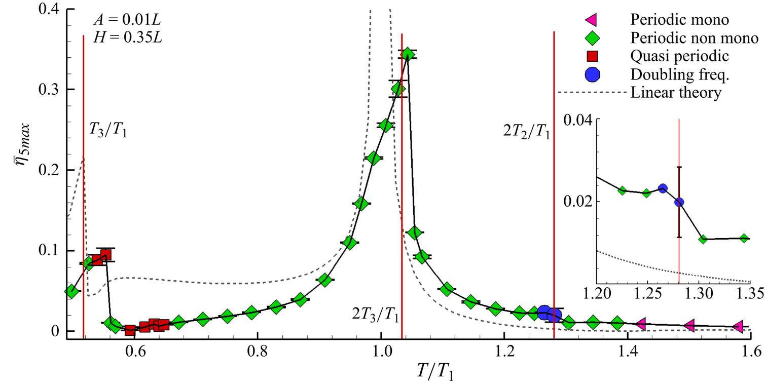
Figure 4. The WEFDs for tank oscillations of 0.01 m and varying frequency with different symbols and colours the different regimes. For every point, the standard deviation is indicated with a vertical error bar. In the legend, the reference to different wave elevation time signals is marked. Left triangle: periodic monochromatic signal. Diamond: periodic non-monochromatic signal. Square: quasi-periodic signal. Circle: doubling-frequency mode. Dashed: linear theory prediction.
As clarified in Faltinsen & Timokha (Reference Faltinsen and Timokha2001), the maximum surface elevation is not obtained for  $T=T_1$, as expected from the theoretical predictions of the linear theory described in Ibrahim (Reference Ibrahim2005), where the free-surface elevation is expressed as a sine expansion.
Faltinsen et al. (Reference Faltinsen, Rognebakke, Lukovsky and Timokha2000) demonstrated that nonlinear effects modify the WEFDs similarly to soft-spring solutions of the Duffing equation (Kovacic & Brennan Reference Kovacic and Brennan2011) when the filling height  $h$ is greater than the critical depth (while for $h$ less than critical depth the WEFDs changes like a hard-spring solution; see e.g. Antuono et al. Reference Antuono, Bouscasse, Colagrossi and Lugni2012a; Bouscasse et al. Reference Bouscasse, Antuono, Colagrossi and Lugni2013).
The dynamic behaviour of soft spring described by Faltinsen et al. (Reference Faltinsen, Rognebakke, Lukovsky and Timokha2000) is also discussed in Colagrossi (Reference Colagrossi2005) for sloshing experiments near the critical depth. The amplitude response vs the oscillation period shows two stable branches with a turning point between them. The set of turning points for different excitation amplitudes defines jumps from the lower to the upper branch and can be found from a cubic secular equation given in Faltinsen et al. (Reference Faltinsen, Rognebakke, Lukovsky and Timokha2000).
The WEFD resulting from linear theory is drawn in figure 4 with a dashed line, where the theoretical predictions are taken from the book of Ibrahim (Reference Ibrahim2005). The departure from linear theory of numerical WEFDs, shown in figure 4, is actually due to nonlinear effects. In particular, in that figure the abscissas relating to  $T=T_3$, $2T_3$, $2T_2$ (see formula (2.1)) are highlighted with vertical lines.
The peak on the left side is related to the resonance of the third sloshing mode, whose period is  $T_3=0.517T_1$. Nonlinear effects lower the amplitude of $\bar {\eta }_{5\max }$ to ${\approx }0.1$ and shift the period to $T \approx 0.55T_1$.
The first sloshing mode leads to a maximum peak of the WEFD observed at  $T=1.044T_1$ with $\bar {\eta }_{5 max} \approx 0.344$. It should be emphasized that the mode $2T_3$ is very close to the first resonance, as highlighted in figure 4, so a combination between $T_1$ and $2T_3$ is a possible explanation for the rightward bending of the WEFD peak.
The second mode, and in general all the even modes, is not directly excited when the tank moves horizontally, but it appears because of nonlinear effects. From the WEFD in figure 4, a little jump in the low-frequency (i.e. long period) branch is found at  $T=2T_2$, where $T_2=0.64T_1$ is the second sloshing period. The jump is evidenced with a magnification of the WEFD in the range $T\in [1.2T_1\unicode{x2013}1.35T_1]$.
Once the sloshing amplitude is assigned, different sloshing regimes are observed for different frequencies and they are indicated in figure 4 with different symbols (similar to Durante et al. Reference Durante, Rossi and Colagrossi2020). The regimes found at the smallest amplitude ( $A=0.01L$) are: periodic monochromatic, periodic non-monochromatic, doubling-frequency and quasi-periodic regimes. Figure 5 shows the time histories and the corresponding Fourier transform spectra of $\eta _5$ for four different cases:
(i)
$T=1.50T_1$ periodic monochromatic;(ii)
$T=1.01T_1$ periodic non-monochromatic;(iii)
$T=1.28T_1$ doubling-frequency mode;(iv)
$T=0.55T_1$ quasi-periodic mode.


Figure 5. Time signals (a,b,c,d) and corresponding Fourier transform spectra (e,f,g,h) for different sloshing regimes at oscillation amplitude of 0.01 m; (a,e)  $T/T_1=1.50$ – periodic monochromatic, (b,f) $T/T_1=1.01$ – periodic non-monochromatic, (c,g) $T/T_1=1.28$ – doubling frequency, (d,h) $T/T_1=0.55$ – quasi-periodic. The non-dimensional frequency is $f^* = T f$. The blue circle indicates the amplitudes related to first natural frequency $f^*_1=T/T_1$.
At low frequencies  $(T> 1.4T_1)$ $\eta _5$ behaves as a monochromatic signal. As shown in panel (a,e) of figure 5, the time signal resembles a simple sinusoidal function and, indeed, the Fourier transform shows a single dominant peak at $f^* = T f = 1$. The blue circle at $f_1^* = T/T_1 = 1.50$ represents the natural oscillation frequency of the tank and it is dominant during the transient. In the selected time window, the latter is lower than $10^{-4}$, so that it can reasonably be assumed negligible and the regime may be considered as unaffected by the transient spurious components.
Increasing the oscillation frequency, a periodic non-monochromatic time signal appears. In figure 5(b,f) the signal at  $T = 1.01T_1$, where the oscillation frequency is forced close to the first resonance, is shown. The Fourier transform shows a main peak, corresponding to the excitation frequency, at $f^*=1$ and a sharp peak at every integer multiple.
When the excitation period  $T$ is such that $T= 2T_2$, the second even mode appears because of nonlinear effects. This mode leads to the onset of a doubling-frequency bifurcation, clearly visible in figure 5(c,g), where the time signal $\eta _5$ presents two peaks in a period. As a consequence, a second peak at $f^*=2$, the intensity of which is comparable to the one at $f^*=1$, occurs in the Fourier transform. Similarly, nonlinear effects induce a similar behaviour for $f^*=3$ and $f^*=4$.
At high frequency, when the period  $T$ is close to $T_3$, a quasi-periodic regime is achieved. A quasi-periodic signal is a periodic signal modulated by a chaotic component (see e.g. Bailador, Trivino & van der Heide Reference Bailador, Trivino and van der Heide2008; Durante et al. Reference Durante, Giannopoulou and Colagrossi2021). In figure 5(d,h), the time signal and the Fourier transform of $\eta _5$ is shown at $T = 0.55 T_1$. The Fourier transform presents a dominant peak for $f^*=1$ while the rest of the spectrum is continuous, typical of chaotic signals (see e.g. Durante et al. Reference Durante, Rossi and Colagrossi2020, Reference Durante, Giannopoulou and Colagrossi2021; Durante, Pilloton & Colagrossi Reference Durante, Pilloton and Colagrossi2022).
The final motion of the tank is attained after a ramp, during which, besides the forcing frequency  $1/T$, a continuous spectrum of modes is excited. The first natural mode (i.e. the first resonance) of period $T_1$ is the most energetic (among them) during the initial transient phase, while the others typically weaken rather quickly, unless they are strengthened by mutual nonlinear interactions. In fact, the first natural mode behaves like a modulation of the time signals that, in some cases, decays after long transients during which the corresponding component remains as a distinct peak in the Fourier spectrum. To demonstrate that the simulations are long enough to make this effect negligible within the analysed time windows, a blue dot corresponding to the amplitude of the first natural mode is drawn in the Fourier spectra of figure 5. As visible, it is always associated with amplitudes approximately 2 orders of magnitude smaller than the amplitude of the excitation frequency.
Figure 6 shows the phase maps  $(\eta _5,\dot {\eta }_5)$. For case $(a)$ the periodic monochromatic signal is represented, as expected, by an elliptical orbit in figure 6(a). Panel (b) of figure 6 reports the phase map of case $(b)$, where the periodic non-monochromatic behaviour leads to an orbit that is an elliptical shape distorted by the nonlinearities. The thickness of the set of curves indicates the presence of a weak modulation that does not preserve a single stable orbit. The doubling-frequency regime of case $(c)$ is represented in figure 6(c) by a knotted orbit with the internal little loop relating to the lower peak within the signal period. The quasi-periodic phase map, case $(d)$, is shown in figure 6(d) and is characterized by nearly circular orbits, where the unpredictable amplitude modulation gives rise to a severe scattering of the same.

Figure 6. Phase maps for different sloshing regimes at oscillation amplitude of 0.01 m. Cases (a,d) of figure 5 on the left and cases (b,c) on the right.
Finally, in figure 7, three configurations of the free surface for the different regimes analysed are schematized. Being trivial, the monochromatic case  $(a)$ is not shown. Cases $(b)$, $(c)$ and $(d)$ are shown in the left, central and right panels of the figure, respectively. Case $(b)$, close to the first resonance, shows large amplitudes of the free-surface oscillations. Case $(c)$, in which the second natural mode is excited, exhibits a central wave relating to the wavenumber $k=2{\rm \pi} /L$. Case $(d)$, in which a quasi-periodic regime is reached, is characterized by an oscillation period $T$ close to the third natural period $T_3$. As a result, waves with wavenumber $k=3{\rm \pi} /L$ develop. The steepness of these waves is quite high and leads, during some cycles, to breaking events. As clarified in Antuono et al. (Reference Antuono, Bardazzi, Lugni and Brocchini2014), the wave breaking causes a partial redistribution of the flow energy over a continuous frequency spectrum, resulting in a chaotic dynamics. As a result, the quasi-periodic behaviour of the time signal $\eta _5$ follows.

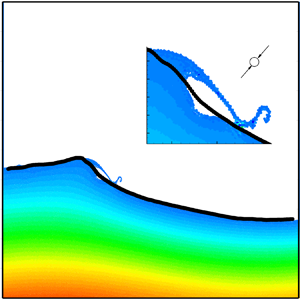
Figure 7. Free-surface evolution for different sloshing regimes at oscillation amplitude of 0.01 m. From left to right: cases (b–d) of figure 5. The time evolution is depicted through colours in the temporal sequence: red, green and blue.
4.2. Amplitude $0.03L$

Experimental and numerical campaigns were carried out for  $A=0.03L$. The numerical and experimental WEFD is drawn in figure 8, together with the identification of the different regimes, given consistently with the classification of § 4.1. For comparison, the theoretical WEFDs resulting from the adaptive multimodal method (AMM) of Faltinsen & Timokha (Reference Faltinsen and Timokha2001) is overlaid on the experimental and numerical results. Although the AMM curve refers to $A=0.025L$, it is still included because no significant differences are expected with respect to the amplitude $A=0.03L$ adopted in the experiments and it is helpful to the discussion. The AMM based on potential-flow model is unable to account for singular events such as breaking or wave impacts, so high-frequency cases cannot be adequately predicted. Despite this, as visible by the dashed line of figure 8(a), the numerical results are quite close to the multimodal data, at least in the range $T/T_1 \in [0.67\unicode{x2013}1.6)$. Regardless of the slightly different reference amplitude, the multimodal curve exhibits a bifurcation around $T = 1.1T_1$ and a doubling-frequency jump at $T=2T_2$ (for a more detailed discussion see also Faltinsen & Timokha Reference Faltinsen and Timokha2009). In contrast, the numerical results reveal a chaotic surface elevation time signal in the range $T/T_1 \in [0.50\unicode{x2013}0.67)$, where the multimodal solution shows a high peak related to the third resonance $T_3/T_1$ and is therefore unable to predict such behaviour.

Figure 8. The WEFDs for tank oscillations of 0.03 m and varying frequency. With different symbols and colours for the different regimes. (a) Numerical simulations. (b) Experiments. In the legend, the reference to different wave elevation time signals is marked. Left triangle: periodic monochromatic signal. Diamond: periodic non-monochromatic signal. Square: quasi-periodic signal. Circle: doubling-frequency mode. Dashed: linear theory prediction.
Figure 8(b) reports the comparison between the experimental data and the multimodal approach.
In the period ranges  $T/T_1\in (0.79,1.00)$ and $T/T_1\in (1.14,1.34)$, the numerical results are in good agreement with the experimental data in terms of mode classification, value of $\bar {\eta }_{5 max}$ and its related standard deviation. In particular, the doubling-frequency regime is found experimentally and numerically near $T=2T_2$, similarly to what was observed for amplitude $A=0.01L$, discussed in § 4.1. At $T=0.867T_1$, a tripling-period bifurcation is identified by both $\delta$-LES-SPH and experiments. This peculiar case and some aspects related to its nonlinear behaviour are discussed in § 5 with the aid of the Hilbert–Huang transform.
In order to stress better the similarities between numerical predictions and experimental data, figure 9 compares the free surface extracted from camera acquisitions with the  $\delta$-LES-SPH particle configuration at $T=0.944 T_1$. Two different time instants were considered, corresponding to the most leftward and most rightward tank positions. Unlike figure 7, where the particle positions were purged by the movement of the tank, here, the latter is explicitly shown. The agreement is rather good, with small discrepancies mainly linked to breaking events typical of the quasi-periodic regime.

Figure 9. Test case A = 0.03L,  $T/T_1$ = 0.944, corresponding to a quasi-periodic regime. Colours are representative of the $\delta$-LES-SPH pressure field. Black dots are the free surfaces extracted by the experimental video.
Although the experimental/numerical comparisons are generally in good accordance, at  $T=2T_3$ the experiments show a second tripling-period scenario not found with the numerical simulations. The disagreement is mainly related to 3-D effects, in fact, the fragmentation of the free surface is more intense in the experiments than in the 2-D simulations. Indeed, the fragmentation induces extra dissipation phenomena which are responsible for the lower value of $\overline {\eta _5}$. Similarly, the highest points of the WEFDs at $T=1.067 T_1$ and $T=1.107 T_1$ of the experimental data are approximately 13 % lower than the $\delta$-LES-SPH results. This point is dealt with in § 6, where a 3-D simulation is also discussed.
Figure 10 shows the experimental and numerical time histories and the related Fourier transforms for case  $T=1.107T_1$ (a,b) and $T=0.867T_1$ (c,d). As commented above, the numerical simulation represented in ( $a$) presents a more energetic signal with respect to the experimental one, shown in ( $b$). A quasi-periodic regime is attained for both signals, as evidenced by the Fourier spectrum, where dominant peaks overlap with an almost continuous spectrum, as it is typical of a chaotic modulation.

Figure 10. Time signals (left) and corresponding Fourier transform spectra (right) for different sloshing regimes at oscillation amplitude of 0.03 m; (a)  $T/T_1=1.10$ – quasi-periodic numerical simulations, (b) $T/T_1=1.10$ – quasi-periodic experiments, (c) $T/T_1=0.867$ – tripling-period numerical simulations, (d) $T/T_1=0.867$ – tripling-period experiments. The non-dimensional frequency is $f^* = T f$.
The case  $T=0.867T_1$, close to the period $T=2T_4$, corresponds to a tripling-period scenario. The numerical and experimental time histories are reported in panels ( $c$) and ( $d$) of figure 10, respectively. These signals look very similar to each other, although some differences in peak height are visible, leading to a larger standard deviation for $\delta$-LES-SPH. The tripling-period mode is characterized by a periodic sequence with period $3T$, characterized by three local maxima. This behaviour is reflected in the Fourier transform where, in addition to the peak at the excitation period $T$, two other peaks appear at lower frequencies. As better explained in § 5, the nonlinear combination of three frequency components also excites other high-frequency harmonics, thus leading to the peaked shape of the Fourier spectra.
The phase maps  $(\eta _5, \dot {\eta }_5)$ relating to the previous regimes are depicted in figure 11. In figure 11(a), a quasi-periodic map is drawn for $T=1.107T_1$. The orbit related to the excitation period $T$ is perturbed by a chaotic modulation and the final orbit appears diffused in a thick annular region and affected by evident fluctuations. In pane; (b) of the same figure, the tripling-period regime at $T=0.867T_1$ is characterized by three concatenate orbits. Again the orbits are characterized by diffusion and fluctuations mainly related to wave breaking events, as further commented below.

Figure 11. Phase maps for different sloshing regimes from numerical simulations at oscillation amplitude of 0.03 $L$. (a) Quasi-periodic. (b) Tripling period.
For this latter case, figure 12 depicts the free surface extracted by camera acquisition and compares it with the simulated SPH particles at four time instants.

Figure 12. Test case  $A=0.03L$, $T/T_1 = 0.867$, corresponding to a tripling-period regime. Colours are representative of the $\delta$-LES-SPH pressure field. Black dots are the free surfaces extracted from the experimental video. The video of the simulation is available at Link Video N1.
It is worth noting that, in the  $\delta$-LES-SPH, plunging breaking waves are developed, while in the experiments only spilling breakers are found. These differences are likely related to the fact that the friction effects of the lateral walls in the experiments are missing in the present 2-D simulations as the surface tension effects are neglected in the numerical model; indeed, as shown in figure 12(d), the thickness of the plunging jet is lower than 1 cm.
Again for the case  $T=0.867T_1$, the $\delta$-LES-SPH free surface at four the time instants is depicted in figure 13. The initial time $t_0$ is selected when a plunging breaking wave appears close to the left side of the tank: the panels are related to instants $t_0$, $t_0+T/2$, $t_0+T$ and $t_0+3T/2$.

Figure 13. The  $\delta$-LES-SPH free-surface evolution for the case $A=0.03L$, $T/T_1 = 0.867$, corresponding to a tripling-period bifurcation. The plots are in the tank reference frame.
Following the time sequence, the breaking wave changes side after a time interval equal to  $T + T/2$. This means that the wave should appear again close the left side of the reservoir at $t=t_0+3T$ and this is the key phenomenon behind the three rising maxima in a single period of $\eta _5(t)$ time signal.
Finally, figure 14 reports the phase map for three other cases. Panel (a) refers to the high-frequency case  $T=0.593T_1$ for which the orbit is fully chaotic, without showing any clear attractor. Looking at the WEFD in figure 8, the experimental data are not available in the high-frequency region ( $T< T_2$), therefore, this region is studied only numerically and the six simulations carried out are all classified as chaotic. This behaviour comes from the intensification of breaking phenomena which also caused an asymmetric behaviour between $\eta _5$ and $\eta _{95}$. This latter appears as a series of water impacts hitting one side only of the tank during certain time ranges, the span of which varies randomly during the flow evolution. This peculiar phenomenon is better discussed in § 7.

Figure 14. Phase maps for different sloshing regimes from numerical simulations at oscillation amplitude of 0.03 $L$. (a) Chaotic. (b) Periodic non-monochromatic. (c) Periodic non-monochromatic. (d) Doubling frequency.
The second and third phase maps of figure 14 refer to (b) and (c), where a periodic non-monochromatic mode is attained. Sharp orbits affected by negligible diffusion are visible. In particular, (b) ( $T=0.791T_1$) shows an orbit very similar to an ellipse, indicating that nonlinear effects play a negligible role. In contrast, the case $T=1.138T_1$, considered in (c), is characterized by a more deformed orbit.
Finally, the phase map of the doubling-frequency mode ( $T=1.304T_1$) is shown in (d) and depicts two concatenate orbits, as expected.
5. Tripling-period and doubling-frequency modes analysed with the Hilbert–Huang transform
In the present section the Hilbert–Huang transform (HHT) is used to make some aspects related to doubling and tripling modes more clear. The HHT was designed for nonlinear and non-stationary signals (Huang et al. Reference Huang, Shen, Long, Wu, Shih, Zheng, Yen, Tung and Liu1998) and it works by two successive steps: the empirical mode decomposition (EMD) and the Hilbert transform (HT). The EMD is used to decompose a signal into a number of intrinsic mode functions (IMFs). An IMF is an oscillatory function with time-varying frequencies that represents the characteristics of non-stationary signals (Lee et al. Reference Lee, Chang, Hsieh, Deng and Sun2012).
In the time range  $[t_1-t_2]$ the reference signal $X(t)$ is expressed as a combination of IMFs as
 \begin{equation} X(t) = \displaystyle{\sum_{i=1}^n} \,\mbox{IMF}_i(t) + \mathcal{R}_n(t), \end{equation}
where  $n$ is the total number of IMFs and $\mathcal {R}_n(t)$ is the residue function. It is worth noting that, from a theoretical point of view, IMFs are not strictly orthogonal, although this property is actually satisfied, as verified a posteriori.
The HT  $\mathcal {H}$ of IMF $(t)$ consists of a convolution with the Cauchy kernel $k(t)=1/{\rm \pi} t$
 \begin{equation} \mathcal{H}(\mbox{IMF}_k(t))={\frac {1}{{\rm \pi} }} \,{\int\hskip -1,05em -\,} _{-\infty }^{+\infty }{\frac {\mbox{IMF}_k(\tau )}{t-\tau }}\,\mathrm {d} \tau \quad\mbox{with} \ k = 1, \ldots, n, \end{equation}
where the principal value of the integral is considered. The signal  $X(t)$ is represented in the complex plane with the function $\boldsymbol {Z}(t)$ (complex quantities are indicated in bold) defined as
 \begin{equation} \left.\begin{gathered} \boldsymbol{Z}_k(t) = \mbox{IMF}_k(t) + \boldsymbol{i} \mathcal{H}(\mbox{IMF}_k(t))= A_k(t) \exp{[ \boldsymbol{i} \theta_k(t) ]} \quad \mbox{with} \ k = 1, \ldots, n \\ A(t) = |\boldsymbol{Z}(t)| , \quad f(t) = \displaystyle{\frac{1}{2 {\rm \pi}} \,\frac{{\rm d}\theta(t)}{{\rm d}t}} \quad \mbox{with} \ \theta(t) = \angle{\boldsymbol{Z}(t)} \end{gathered}\right\}, \end{equation}
with  $\boldsymbol {i} = \sqrt {-1}$, $A(t)$ the instantaneous amplitude and $f(t)$ the instantaneous frequency of $\boldsymbol {Z}(t)$.
The time behaviours of the frequencies of different IMFs, made non-dimensional with the excitation frequency  $f_e=1/T$, are drawn in figure 15 for $T=1.304 T_1$ and in figure 17 for $T=0.867 T_1$. These cases correspond to a doubling-frequency and to a tripling-period bifurcations, respectively. In order to highlight the most energetic modes, the curves are contoured with the non-dimensional amplitude $A(t)/L$. The ordinate $f^*=fT$ refers to dimensionless frequencies, so the dimensionless excitation frequency $f_eT$ is 1 by definition. Considering that the numbering of IMF modes is arbitrary, we decided to number the modes by their energy content, so that the mode IMF $_1$ is the most energetic and so on.

Figure 15. Hilbert transform for the case  $A=0.03 L$ and $T=1.304 T_1$. The different lines correspond to the time trends of the frequencies related to the different modes. The lines are contoured with the amplitudes of the corresponding modes for varying $t$. The frequencies are non-dimensional with the exciting carrier $1/T$.
Since the energy of  $X(t)$ is in general roughly equal to the sum of the energies of its modes, the distribution of the signal energy among IMF modes is discussed. It is worth underlining that, with a little abuse of language, we will refer in the following to the mode energy, although we are actually dealing with its amplitude.
Figure 15 represents the time trends of IMF mode frequencies at  $T=1.304 T_1$, where a doubling-frequency scenario occurs. Although the system is excited at frequency $f_e$, a significant part of the energy moves to $2 f_e$, making this mode comparable, in terms of energy, to the first harmonic. This happens because the second harmonic of the excitation frequency is close to the second resonance, i.e. $2f_e \sim f_2=1/T_2$, as indicated by the formula (2.1). This induces an energy transfer toward $2 f_e$, similarly to what observed by Wu (Reference Wu2007), who performed similar investigations with a linear perturbation theory. The second mode is excited by nonlinearity so that, in figure 15, it is possible to appreciate that the mode IMF $_1$, related to frequency $2f_e$, starts at approximately 10 oscillation periods and it persists over time without appreciable perturbations. With analogous arguments, modes IMF $_3$ and IMF $_4$, linked to frequencies $3 f_e$ and $4 f_e$, become rather similar as well. The final emerging pattern is typical of a doubling-frequency regime. Figure 16 shows the time histories of the sum of the first two IMFs ${\rm IMF}_1+{\rm IMF}_2$. The plot depicts the onset and the persistence of the doubling-frequency regime.

Figure 16. Sloshing case  $A=0.03 L$ and $T=1.304 T_1$: time histories of the sum of the first two IMFs ${\rm IMF}_1+{\rm IMF}_2$ calculated from the $\delta$-LES-SPH $\eta _5$ time signal.
The case  $T= 0.867 T_1$, where a tripling-period bifurcation occurs, is more complex. As shown in figure 17, the mode ${\rm IMF}_1$ related to the excitation frequency $f_e$ rapidly appears and persists as almost constant in time. The mode ${\rm IMF}_4$, related to first resonance $f_1 = 1/T_1$, arises during the early periods of oscillation as an effect of the initial ramp used for the simulation but, after roughly $40$ oscillations, the mode is almost totally damped with an amplitude that becomes negligible.

Figure 17. Hilbert transform for the case  $A=0.03 L$ and $T=0.867 T_1$. The different lines correspond to the time trends of the frequencies related to the different modes related to the $\delta$-LES-SPH $\eta _5$ signal. The lines are contoured with the amplitudes of the corresponding modes for varying $t$. The frequencies are made non-dimensional with the exciting carrier $1/T$.
The second and third sloshing natural frequencies (i.e.  $f_2 = 1/T_2$ and $f_3 = 1/T_3$, respectively) are, in this case, related to $f_e$ as $f_2 \sim f_e + 1/3 f_e$ and $f_3 \sim f_e + 2/3 f_e$. This implies that, when the energy of ${\rm IMF}_4$ is redistributed among other frequencies, it falls on modes ${\rm IMF}_2$ and ${\rm IMF}_5$, corresponding to $f_2$ and $f_3$. These latter become energetic enough to persist in time and to become sub-harmonics between $f_e$ and $2 f_e$. The modes ${\rm IMF}_2$ and ${\rm IMF}_5$ interact with ${\rm IMF}_3$, making the modes related to sub-harmonics $2 f_e - f_2 \sim 2/3f_e$ and $2 f_e - f_3 \sim f_e/3$ to appear. The final frequency spectrum attained by the system assumes the typical peaked shape of a tripling-period one (see figure 10c).
Figure 18 shows the time histories of the sum of the first two IMFs  ${\rm IMF}_1+{\rm IMF}_2$. The plot depicts the onset and the persistence of the tripling-period regime.

Figure 18. Sloshing case  $A=0.03 L$ and $T=0.867 T_1$: time histories of the sum of the first two IMFs ${\rm IMF}_1+{\rm IMF}_2$ calculated from the $\delta$-LES-SPH $\eta _5$ time signal.
Finally, the case at  $T= 1.022 T_1$ is depicted in figure 19, where the experimental outcomes and the numerical solution are compared. As shown in panel (a) of the figure, the analysis of the experimental result shows a dynamics very similar to $T=0.867 T_1$, discussed above. The mode corresponding to $f_1$ appears during initial oscillation periods, caused by the ramp, and rapidly damps out. The energy is then redistributed among other frequencies and the tripling-period pattern forms again, similarly to that just observed in figure 17. Conversely, the 2-D restriction assumed in the numerical simulations leads here to a discrepancy. The energy of mode related to frequency $f_1$ remains confined to its initial state and does not spread among other frequencies, although it starts to oscillate chaotically.

Figure 19. Hilbert transform for the case  $A=0.03 L$ and $T=1.022 T_1$. The different lines correspond to the time trends of the frequencies related to the different modes. The lines are contoured with the amplitudes of the corresponding modes for varying $t$. The frequencies are non-dimensional with the exciting one $1/T$. (a) Experimental data, (b) $\delta$-LES-SPH outcome.
This plays the role of a chaotic modulation of the carrier signal, giving rise to a quasi-periodic pattern. For this reason, a tripling-period regime is not attained. This discordance between 2-D SPH simulations and experimental data is further discussed in § 6.
6. Tripling-period regime at $A=0.03L$ and $T= 1.022 T_1$: 2-D vs 3-D comparison


In § 5, the doubling and tripling bifurcations appearing in the WEFDs are discussed and investigated through the HHT. For  $A=0.03L$ and $T = 1.022 T_1$, a discrepancy between numerical and experimental evidence is found and a tripling-period behaviour of the time signal appears from experiments, whereas numerical simulations provide a quasi-periodic mode prediction. In order to find a reason for this discrepancy, we first try to change the solid boundary condition on the tank wall. However, in this particular test case the 2-D solutions appear to be not so influenced by those changes even when a free-slip condition is considered.
The disagreement between numerical and experimental data is presumably due to the 2-D restriction, however, in order to gain a deeper insight into this problem, 3-D simulations have been carried out with a  $\delta$-LES-SPH model and the results are shown in figure 20 in terms of the surface elevation time signal, and in figure 21 in terms of the free-surface evolution. The resolution used for the simulation is $N=H/\Delta r=50$, which means approximately 100 000 particles in the whole numerical domain. A free-slip boundary condition was used on the tank walls, thus avoiding the discretization of the boundary layers, in particular at low spatial resolutions (i.e. $N=50$). After many tests, this assumption was found accurate enough in two dimensions, thus it was adopted also in three dimensions.

Figure 20. Time histories of the surface elevations  $\eta _5$ for the case $A=0.03 L$ and $T/T_1=1.022$. Solid line: experimental data; dashed line: 3-D $\delta$-LES-SPH simulation. Letters A,B,C and D identify the time instants for the particle displacements sketched in figure 21.

Figure 21. Free-surface evolution for the case  $A=0.03 L$ and $T=1.022 T_1$ obtained with 3-D $\delta$-LES-SPH simulations.
The significant increase in computational costs did not allow a long simulation time, thus the simulation is limited to  $t=100 T$ and, for the same reasons, the present investigation, including approximately 230 simulations, cannot be carried out within a 3-D environment.
Figure 20 shows a comparison between  $\delta$-LES-SPH and the experimental time history of the surface elevation recorded by the probe $\eta _5$. From this plot it is possible to appreciate that, unlike the 2-D simulation, the 3-D numerical simulation is able to identify the tripling-period regime. In table 1, the comparisons among the values of $\bar {\eta }_{5 max}$ from 2-D and 3-D simulations and experiments is detailed. The average maximum of the 3-D numerical signal differs by approximately $2.5\,\%$ from the experiments, whereas the difference grows to $35.7\,\%$ with the 2-D simulation.
Table 1. Comparisons in terms of  $\bar {\eta }_{5 max}$ from 2-D and 3-D simulations and from experimental outcomes. The standard deviations are also indicated in the rightmost column.

Figure 21 displays the lateral view of the particle configuration at four time instants. Particles are coloured with pressure. From this figure, it is possible to recognize the occurrence of the breaking waves which characterize the tripling-period regime, as already discussed in § 4.2.
Figure 22 shows the images recorded by the digital camera at the same instants as figure 21. The main flow features recorded by the digital camera are well predicted by the numerical solvers. As already mentioned, this pattern does not appear in two dimensions, indicating that, for this specific case, the transverse velocity component plays a key role because of the fragmentation of the free surface.

Figure 22. Digital images for the case  $A=0.03 L$ and $T=1.022 T_1$ at the same time instants as figure 21.
7. Asymmetric regimes
For the problem of sloshing in a tank, Olsen (Reference Olsen1970) tacitly assumed a global symmetry between the left and right sides of the tank. Intuitively, this seems reasonable because the tank is a cuboid moving laterally leftwards and rightwards, so there is no reason for which any asymmetry should appear. For an oscillation period  $T$, the right probe should record the same signal as the left one, but delayed by $T/2$. Unexpectedly, Colagrossi (Reference Colagrossi2005), Colagrossi et al. (Reference Colagrossi, Palladino, Greco, Lugni and Faltinsen2006) and Faltinsen & Timokha (Reference Faltinsen and Timokha2009) found that, at high motion amplitudes, the left $\eta _L$ and the right $\eta _R$ probes do not measure similar signals. In the present section, the presence of signal asymmetries is numerically addressed.
In order to have a quantitative evaluation of the asymmetry, a measure of the left and right probe cross-correlation is computed for each case. The correlation function is defined as (Stoica & Moses Reference Stoica and Moses2005)
 \begin{equation} R_{[ \eta_L \ \eta_R ]}(m) = \displaystyle{\sum_{k=1}^{N-m-1}} \eta_L(t_k + m \Delta t) \eta_R(t_k) \quad \mbox{with} \ t_k = t_0 + k \Delta t, \end{equation}
where  $\Delta t$ is the time discretization of the signals and $m \Delta t$ is the time delay between signals. Varying the parameter $m$, the maximum value $R_{[ \eta _5 \ \eta _{95} ]}^*$ is considered. In order to get a meaningful value, the normalized cross-correlation is used
 \begin{equation} \hat{R}_{[ \eta_L \ \eta_R ]} = 1 - \displaystyle{\frac{ R_{[ \eta_L \ \eta_R ]}^* }{ \sqrt{ R_{[ \eta_L \eta_L ]}(0) \ R_{[ \eta_{R} \ \eta_{R} ]}(0) } }} . \end{equation}
For two identical signals,  $\hat {R}_{[ \eta _L \ \eta _R ]}$ is equal to 0, while it tends to 1 for two non-correlated signals. As reported in figure 23 in the range $T\in (0.5 T_1, 0.7 T_1)$, the left and right probes are less correlated than in the rest of the range. In particular, for an oscillation amplitude of $A=0.03L$, the maximum asymmetry is attained for chaotic modes and specifically for the case $T=0.593 T_1$. Conversely, for $A = 0.01L$ the maximum of asymmetry is attained for quasi-periodic regimes.

Figure 23. Cross-correlation distribution with frequency for  $A=0.01 L$ and $A=0.03 L$.
An example of a non-symmetric mode for  $A = 0.03L$ is shown in figure 24, where the acquisitions of the free-surface elevation $\eta _1$ for the left side and $\eta _{99}$ for the right side of the tank are compared. The full signals are shown in the top panel of the figure, whereas a magnification of the range $t\in (125T,128T)$ is given at the bottom: the vertical lines correspond to time instants at which the free surface is depicted in figure 25. As visible, the left side (orange solid) and the right side (black dash-point) signals are different and the intensity of the elevation switches between left and right after intervals of approximately $50\unicode{x2013}70$ oscillation periods. In figure 24(b), for example, the right side elevation is higher than the left side.

Figure 24. (a) Time histories of the surface elevations from the left probe  $\eta _1$ and the right probe $\eta _{99}$ for the chaotic case $A=0.03 L$ and $T/T_1=0.5$. (b) Enlarged view of the time history for the probe $\eta _{99}$ within the time range $t\in [125T,128T]$. Left probe signal is drawn with the orange solid line, right probe with the black dash-point line. Vertical dashed lines correspond to time instants selected for the free-surface configurations of figure 25 and letters refer to related panels.

Figure 25. Chaotic case  $A=0.03 L$ and $T/T_1=0.5$: free-surface configuration for 9 different time instants in two periods of the tank oscillations $t\in [125.75T, 127.75T]$. To improve the visibility $y^*$ is equal to $y$ for the red points, and equal to $y^*=y+0.15$ and $y^*=y+0.3$ for the green and blue points, respectively. Red points correspond to the configuration where $\eta _{99}$ is close to its maximum values of figure 24(b). Red arrows indicate the direction of the tank motion. The video of the simulation is available at Link Video N2.
The free surface shows different patterns when the tank is moving leftwards and rightwards. With respect to the interval highlighted in figure 24(a), when the free surface impinges on the left side of the tank and moves rightwards, a breaking wave is formed (see blue lines in figure 25). The same pattern is not formed when the free surface moves leftwards, as indicated by red lines in the same figure.
8. Sloshing dissipation
In the present section the slosh dissipation is addressed. As underlined in Colagrossi, Bouscasse & Marrone (Reference Colagrossi, Bouscasse and Marrone2015), the dissipation is linked to two main phenomena: (i) the wall boundary layer (WBL) near the tank walls and (ii) complex motions of the free surface leading to its fragmentation during breaking waves and wave impact events. These two mechanisms act with different intensity, depending on the attained regimes. Indeed, for the periodic monochromatic regime the motion of the free surface is rather mild and singular phenomena do not occur: as a consequence, the main dissipation comes from the WBL. Conversely, during the quasi-periodic regime, the large motion of the free surface, its fragmentation and the occurrence of water impact events make mechanism (ii) as the dominant one.
It is worth noting that the 2-D assumption does not take into account the viscous friction on the front and rear tank sides, hence, the WBL effects are reduced. In order to partially recover this effect, viscous damping corrections are often used in the literature, following the pioneering work of Keulegan (Reference Keulegan1959). These corrections are generally useful for sloshing flows in shallow water, as discussed in Bouscasse et al. (Reference Bouscasse, Antuono, Colagrossi and Lugni2013) and in Antuono et al. (Reference Antuono, Bouscasse, Colagrossi and Lugni2012a). Unfortunately, this is not the case for the present work, where the problem is in intermediate depth conditions and, for this reason, we preferred to avoid any correction to the fluid viscosity.
As introduced in § 3.3, the energy balance is given by three general terms
 \begin{equation} \mathcal{E}_M-\mathcal{W}_{NF}=\mathcal{E}_{diss}, \end{equation}
where  $\mathcal {E}_M$ is the mechanical energy of the fluid in the Ni-FoR moving with the tank, $\mathcal {W}_{NF}$ is the work performed by the non-inertial forces and $\mathcal {E}_{diss}$ is the energy dissipated by the fluid.
Figure 26(a) shows the time behaviour of the three energy terms for the test case  $A=0.03L$ and $T=0.867T_1$ (tripling-period scenario) evaluated by the $\delta$-LES-SPH model at resolution $N=H/\Delta r=200$. The energies in (8.1) are made non-dimensional with the reference kinetic energy
 \begin{equation} \Delta \mathcal{E}= \displaystyle{\frac{1}{2}} m_l \left( 2{\rm \pi} \displaystyle{\frac{A}{T}} \right)^2 \displaystyle{\frac{t_{end}}{T}}, \end{equation}
that is the maximum kinetic energy of the liquid (imagining it frozen inside the tank) multiplied by the total number of periods. From this figure it is clear that the mechanical energy needs approximately  $N_{P0}=80$ oscillation periods before reaching a constant condition. Similarly, the external work $\mathcal {W}_{NF}$ and the dissipated energy $\mathcal {E}_{diss}$ time trends become almost linear. Within this regime the almost constant time rate of $\mathcal {E}_{diss}$ is defined as the dissipated power $\bar {\mathcal {P}}_{diss}$, which is directly related to the specific case investigated (see (3.14) in § 8).

Figure 26. Test case  $A=0.03 L$ and $T/T_1=0.867$. (a) Time evolution of mechanical energy $\mathcal {E}_M$ (in Ni-FoR), work performed by the non-inertial forces $\mathcal {W}_{NF}$ and dissipated energy $\mathcal {E}_{diss}$. Results refer to $\delta$-LES-SPH simulations at finest spatial resolution $N=H/\Delta r=200$. (b) Time evolution of the energy dissipated by the fluid $\mathcal {E}_{diss}$ at three spatial resolutions $N=50$, 100 and 200. The energies are made non-dimensional with the reference energy in (8.2).
Panel (b) of the same figure depicts  $\mathcal {E}_{diss}$ at three different spatial resolutions. The time trend of the dissipated energy clarifies that, at the finer resolution, the curve slope is convergent; moreover, it is also clear that $\mathcal {E}_{diss}$ is roughly well captured even at the lowest resolution, thus indicating that the present numerical approach is very reliable when energy evaluations are carried out.
By extending the discussion to the whole frequency spectrum and to both sloshing amplitudes, figure 27 shows  $\bar {\mathcal {P}}_{diss}$ as a function of the oscillation periods and for both the motion amplitudes $A=0.01L$ and $0.03L$. The dissipated power is made non-dimensional with the reference power $\Delta \mathcal {P}=\Delta \mathcal {E}/t_{end}$.

Figure 27. Time rate of the dissipated energy distribution with frequency for  $A=0.01 L$ and $A=0.03 L$. Results refer to $\delta$-LES-SPH simulations at the finest spatial resolution $N=H/\Delta r=200$.
The two curves, in logarithmic scale on the vertical axis, follow a similar trend as the WEFDs, discussed in §§ 4.1 and 4.2. It is worth noting that, where the tripling-period and the doubling-frequency modes occur, clearly visible peaks are found. The higher dissipation is linked to the presence of breaking waves and of wave impacts against the vertical walls, developing during the tripling-period and doubling-frequency regimes, respectively. The breaking wave phenomena are also responsible for the increase (in absolute value) of the dissipated power at the lowest excitation periods, where, at  $A=0.03L$, chaotic regimes occur.
Finally, the time histories of the velocity of the fluid centre of mass  $\dot {x}_G(t)$ and of the tank acceleration $a_{tank}(t)$ are depicted in figure 28 for $A=0.03L$ at $T=0.791 T_1$ and $T=1.098 T_1$. The former is one of the cases where the slosh dissipation is very low, hence, $\dot {x}_G(t)$ and $a_{tank}(t)$ are close to quadrature. Conversely, at the excitation period $T=1.098 T_1$ the maximum dissipation is attained and $\dot {x}_G(t)$ and $a_{tank}(t)$ are in anti-phase. Those phase lag conditions are in agreement with the formula (3.14), which links the average slosh dissipation rate $\bar {\mathcal {P}}_{diss}$ with $\dot {x}_G(t)$ and $a_{tank}(t)$.

Figure 28. Test cases  $A=0.03L$, $T=0.791 T_1$ (a), $T=1.098 T_1$ (b) showing time histories of the fluid centre of mass velocity $\dot {x}_G(t)$ and the tank acceleration $a_{tank}(t)$.
9. Conclusions
In the present article the fluid sloshing in a cuboid tank oscillating laterally is investigated. The problem is addressed for a filling height close to the critical depth and for two motion amplitudes, namely  $A = 0.01 L$ and $A = 0.03 L$. A wide span of excitation frequencies is investigated. Numerical simulations have been carried out with a $\delta$-LES-SPH model for both amplitudes, whereas experimental data were also available for larger amplitude. The numerical approach is an improvement of the classic SPH technique widely validated in the literature. By taking into account the time average of the surface elevation maxima, measured near the left wall of the tank, a frequency spectrum is obtained for both amplitudes and different scenarios were identified. Numerical outcomes were compared with experiments, showing a good agreement in terms of the surface elevation time signal and of the sloshing regime. Moreover, with the aid of a high-resolution camera, numerical and experimental free surfaces were overlapped for some interesting cases, showing again a remarkable superposition. Doubling-frequency and tripling-period bifurcations were also found both experimentally and numerically and the mechanism of their onset was discussed with the HHT. For one case, at $A=0.03L$ and $T/T_1 = 1.022$, the tripling-period regime is not attained in 2-D simulations, whereas it appears during the experiments. To dispel any doubts about the possible reasons behind this, a 3-D simulation was carried out and both the same regime and a value of $\bar {\eta }_{5 max}$ very close to the experimental one were recovered. This comparison clarified the effect of the transverse velocity, which induces fragmentation of the free surface leading to an increase of the dissipation mechanisms. The latter lower the mechanical energy of the flow allowing the tripling mode regime.
Left and right numerical probes were provided on sidewalls of the tank, so that the presence of asymmetric regimes has been detected and discussed. The frequency distribution of the cross-correlation between the left and right probes shows that, in some scenarios, particularly where the chaotic regime is attained, the asymmetry makes the signals highly uncorrelated.
Finally, a discussion about the energy dissipation was carried out. As expected, breaking waves or water impact events, typical of quasi-periodic or chaotic regimes, are more dissipative than the WBL, which is the only dissipation source in monochromatic cases. Moreover, also doubling-frequency and tripling-period regimes give higher dissipation than periodic non-monochromatic scenarios.
Although two-dimensional, the present numerical investigation required a significant computational time effort in simulating a very long dynamics which took approximately 2 million iterations to cover 300 seconds of physical acquisition time. An analysis of computational costs concluded that, for a total of 228 simulations, an average computational speed of  $35\ \mathrm {\mu }{\rm s}$ was attained, such requiring approximately 1 week for every fine-resolution simulation.
Future activities will concern sloshing test campaigns for the investigations of higher-amplitude motions.
Funding
The work was partially supported by the SLOWD project, which received funding from the European Union's Horizon 2020 research and innovation programme under grant agreement No. 815044, and partially supported by the Italian ‘Ministero dell'Ambiente e Sicurezza Energetica’ under the Grant Agreement ‘RdS PTR 2022–2024 – Energia elettrica dal mare’. Funding was also received from project ECS00000024 ‘Ecosistemi dell'Innovazione’ – Rome Technopole of the Italian Ministry of University and Research. The simulations were performed by using HPC resources of the Centrale Nantes Super- computing Centre on the cluster Liger. The authors would like to thank Dr P. Sun from Sun Yat-Sen University (School of Marine Engineering and Technology), for his fruitful suggestions and help during the revision stage of this work.
Declaration of interests
The authors report no conflict of interest.
Appendix A. The CPU costs
Although in the present work we carried out only 2-D simulations, the CPU costs are, however, remarkable, since 76 runs were needed to cover the WEFD spectra shown in figure 4 and in figure 8. For each case three runs at spatial resolutions  $N=H/\Delta r=50$, 100 and 200 were performed, for a total of 228 simulations. The number of particles at the finest resolution is only 114 000, however, the long-time simulations performed ( $t_{end}=300$ s) required approximately 2 million time iterations.
The  $\delta$-LES-SPH simulations ran on the ‘Liger’ supercomputer of Ecole Centrale de Nantes, which is equipped with 252 nodes, each one with 12-core Intel Xeon (Haswell) E5–2680v3 processors. The computational speed can be defined as
 \begin{equation} \eta=\frac{CPU_{time}N_{cores}}{N_{iterations}N_{particles}}. \end{equation}
For the present SPH solver, which is an in-house research code with a hybrid OpenMP/MPI parallelization, the computational speed is approximately  $\eta =35\ \mathrm {\mu }{\rm s}$. It follows that, at the finest resolution, each simulation requires approximately one week on a single cluster node. The total computational cost for the whole set of runs requires approximately one month of calculation on 20 computing nodes (i.e. 240 cores).
Appendix B. Effect of the spatial resolutions on the tripling-period regime
In this appendix, the effect of the spatial resolution on the sloshing flows is investigated. As a reference case  $A=0.03L$ and $T=0.867 T_1$ is considered. For this test case a tripling-period regime is identified by the experimental campaign, as already commented on in § 4.2. Four different spatial resolutions $N=H/\Delta r=25, 50, 100, 200$ are considered and 180 oscillating periods were simulated. The convergence of the dissipated energy was already commented on in § 8, whereas the effect of $N$ on the surface elevation $\eta _5$ and on the free-surface displacement is discussed here.
Figure 29 shows the time histories of the surface elevation measured by  $\eta _5$ probe at different spatial resolutions. Only the last 20 oscillations of the tank are considered. As pointed out in § 4.2, the $\delta$-LES-SPH output using $N=200$ is in good agreement with the digital images recorded during the experiments, both in terms of the statistics of the $\eta _5$ signal and particle displacements. In particular, the typical tripling-period patterns are clearly visible in figure 29(d), corresponding to $N=200$. Coarsening the resolution to $N=100$ and $N=50$, the tripling-period patterns are still found, although this is not the case for the lowest resolution $N=25$, where a simple periodic regime is attained.

Figure 29. Test cases  $A=0.03L$, $T=0.867 T_1$: $\delta$-LES-SPH time histories of the surface elevation measured at the $\eta _5$ probe position using four different spatial resolutions, $N=H/\Delta r=25, 50, 100, 200$ (a–d).
The reason behind it relies in the fact that, at the coarsest resolution  $N=25$, the breaking wave events cannot be resolved, as illustrated in figure 30. From the same figure, it is possible to see that, at $N=50$, only spilling breakers appear, while at $N=100$ and $N=200$, plunging breakers clearly develop inside the tank. The surface elevation $\eta _5$, measured at 5 cm from the left wall is not very sensitive to the different breakers developed (spilling or plunging) inside the tank and this clarifies why the $\eta _5$ signals are not much different for spatial resolutions $N=50$, $100$ and 200.

Figure 30. Test cases  $A=0.03L$, $T=0.867 T_1$: particles belonging to the free surface at time $t=164.7T$ using four different spatial resolutions $N=25,50,100$ and 200. The vertical positions of the particles are shifted using the variable $y^*$.
The analysis carried out here has been extended also to other sloshing cases of the present work, in order to check that  $N=200$ is a fine enough resolution for all the simulations considered. The only exception is the chaotic regime, for which the effect of the spatial resolution can be considered in a statically sense only.


 Open access