


1. Introduction
In weakly ionised plasmas, inelastic collisions play key roles in runaway electron (RE) (Wilson Reference Wilson1925) generation by slowing down electrons (Gurevich Reference Gurevich1961) and creating knock-on sources (Rosenbluth & Putvinski Reference Rosenbluth and Putvinski1997). For highly energetic electrons, inelastic slowing down can be adequately described by the Fokker–Planck (FP) operator (Chandrasekhar Reference Chandrasekhar1943; Rosenbluth, MacDonald & Judd Reference Rosenbluth, MacDonald and Judd1957) since the typical energy transfer is much smaller than their energy (Breizman et al. Reference Breizman, Aleynikov, Hollmann and Lehnen2019). Similarly, free-bound knock-on collisions, often approximated as free–free knock-on under the assumption of negligible ionisation potential (McDevitt, Guo & Tang Reference McDevitt, Guo and Tang2019), can be accounted for by the Boltzmann operator (Landau, Lifshitz & Pitaevskij Reference Landau, Lifshitz and Pitaevskij1981; Rosenbluth & Putvinski Reference Rosenbluth and Putvinski1997). The main interest of previous studies on free-bound collision operators (Kirillov, Trubnikov & Trushin Reference Kirillov, Trubnikov and Trushin1975; Mosher Reference Mosher1975; Hesslow et al. Reference Hesslow, Embréus, Stahl, DuBois, Papp, Newton and Fülöp2017, Reference Hesslow, Embréus, Hoppe, DuBois, Papp, Rahm and Fülöp2018; Breizman et al. Reference Breizman, Aleynikov, Hollmann and Lehnen2019; Walkowiak et al. Reference Walkowiak, Jardin, Bielecki, Peysson, Mazon, Dworak, Król and Scholz2022; Savoye-Peysson et al. Reference Savoye-Peysson, Mazon, Bielecki, Dworak, Król, Jardin, Scholz, Walkowiak and Decker2023) has concentrated on the dynamics of energetic electrons to comprehend undesirable disruption REs (Lehnen et al. Reference Lehnen, Bozhenkov, Abdullaev and Jakubowski2008; Martín-Solís et al. Reference Martín-Solís, Loarte and Lehnen2017; Reux et al. Reference Reux2021) due to the danger of triggering plasma instabilities (Snipes et al. Reference Snipes, Parker, Phillips, Schmidt and Wallace2008; Liu et al. Reference Liu, Lvovskiy, Paz-Soldan, Jardin and Bhattacharjee2023) and ability to damage the device (Nygren et al. Reference Nygren, Lutz, Walsh, Martin, Chatelier, Loarer and Guilhem1997; Matthews et al. Reference Matthews2016; de Vries et al. Reference de Vries2023).
Start-up REs (Knoepfel & Zweben Reference Knoepfel and Zweben1975; Knoepfel & Spong Reference Knoepfel and Spong1979; Sharma & Jayakumar Reference Sharma and Jayakumar1988) are well highlighted recently for the upcoming ITER plasma initiation (de Vries & Gribov Reference de Vries and Gribov2019; de Vries et al. Reference de Vries2023) since significant current carried by them complicates the start-up or even leads to failure (Gribov, Kavin & Lukash Reference Gribov2018; de Vries et al. Reference de Vries, Gribov, Martin-Solis, Mineev, Sinha, Sips, Kiptily and Loarte2020; Hoppe et al. Reference Hoppe, Ekmark, Berger and Fülöp2022; Matsuyama et al. Reference Matsuyama, Wakatsuki, Inoue, Yamamoto, Yoshida and Urano2022; Lee et al. Reference Lee2023b , Reference Lee, Aleynikov, De Vries, Kim, Lee, Hoppe, Park, Choi, Gwak and Na2024; de Vries et al. Reference de Vries2025). Yet, the collision models suitable for describing disruption REs may be inadequate for analysing start-up REs. For instance, the energy of start-up REs is insufficient to make use of the first-order Born-approximation (Landau & Lifshitz Reference Landau and Lifshitz2013) essential for the Bethe stopping power (Bethe Reference Bethe1930) and Thomas–Fermi models (Kirillov et al. Reference Kirillov, Trubnikov and Trushin1975; Hesslow et al. Reference Hesslow, Embréus, Stahl, DuBois, Papp, Newton and Fülöp2017). That is, valid collision cross-sections are necessary for both elastic and inelastic collisions. In addition, energy transfer via inelastic collisions is predominantly hard when the incident electron energy is close to the ionisation potential. This necessitates individual inelastic collisions to be accounted for by the binary Boltzmann operator Landau & Lifshitz (Reference Landau and Lifshitz2013). Furthermore, the background Maxwellian assumption needs to be verified under the strong effect of neutrals on electrons to adopt the linearised free–free collision operator (Helander & Sigmar Reference Helander and Sigmar2005).
According to the classical Dreicer kinetics (Gurevich Reference Gurevich1961; Connor & Hastie Reference Connor and Hastie1975), the key phase space region determining the formation of the Dreicer flow is the narrow singular layer across the critical momentum where the energy diffusion drives an upward flow. However, if the critical energy is close to the ionisation potential in cold weakly ionised plasmas, the key region can be wider from the minimum excitation energy to critical energy in which hard inelastic collisions should be considered by the binary Boltzmann operator. Indeed, it was recently elucidated that the binary nature of inelastic collisions allows quasi-frictionless acceleration for some particles and facilitates the Dreicer generation (Dreicer Reference Dreicer1959), yielding significant enhancement in the generation rate (Lee et al. Reference Lee, Aleynikov, De Vries, Kim, Lee, Hoppe, Park, Choi, Gwak and Na2024). The collision operator aided by the correct cross-sections and Boltzmann operator was originally presented by Lee et al. (Reference Lee, Aleynikov, De Vries, Kim, Lee, Hoppe, Park, Choi, Gwak and Na2024) to include this nature when designing a runaway-free reactor start-up scenario with better confidence, where plasma parameters remain far away from the RE generation parametric region. This paper expands on the collision operator by Lee et al. (Reference Lee, Aleynikov, De Vries, Kim, Lee, Hoppe, Park, Choi, Gwak and Na2024) by (i) describing the model development for electron–hydrogen atom collisions in greater detail; (ii) explicitly verifying the background Maxwellian assumption in cold weakly ionised plasmas under the consideration of complete linearised Coulomb operator; and (iii) presenting the numerical method for implementation of this model into kinetic solvers using the finite volume method (FVM).
The paper is organised as follows. In § 2, we present the Fokker–Planck–Boltzmann (FPB) operator with appropriate free-bound collision cross-sections. In § 3, the numerical implementation of this operator will be clarified. In § 4, the operator is applied to solve the Dreicer problem.
2. Kinetic model
The kinetic equation for the electrons is
 \begin{equation} \frac {\partial f_e}{\partial t} + eE\left [ \frac {\mu }{p^2} \frac {\partial }{\partial p} p^2 + \frac {1}{p} \frac {\partial }{\partial \mu } \bigl(1-\mu ^2\bigr) \right ] f_e = \mathcal{C} \{ f_e \}, \end{equation}
where $f_e(p,\mu )$
is the electron distribution function,
$f_e(p,\mu )$
is the electron distribution function, $p$
is particle momentum and
$p$
is particle momentum and $\mu =\cos {\theta }$
is the cosine of pitch-angle
$\mu =\cos {\theta }$
is the cosine of pitch-angle $\theta$
. Suppose the pure weakly ionised plasmas and assume hydrogen is in the ground state. There are two types of interactions depending on colliding species. Charged particles interact with each other through the long-range Coulomb interaction. The FP operator appropriately describes such inverse-square forces (Rosenbluth et al. Reference Rosenbluth, MacDonald and Judd1957); the free–free knock-on collisions (Rosenbluth et al. Reference Rosenbluth, MacDonald and Judd1957; Chiu et al. Reference Chiu, Rosenbluth, Harvey and Chan1998) are negligible due to low ionisation fraction. However, the interaction between an electron and a hydrogen atom is short-range (close) due to the screened charge. We apply the FPB operator to account for electron–hydrogen atom interactions,
$\theta$
. Suppose the pure weakly ionised plasmas and assume hydrogen is in the ground state. There are two types of interactions depending on colliding species. Charged particles interact with each other through the long-range Coulomb interaction. The FP operator appropriately describes such inverse-square forces (Rosenbluth et al. Reference Rosenbluth, MacDonald and Judd1957); the free–free knock-on collisions (Rosenbluth et al. Reference Rosenbluth, MacDonald and Judd1957; Chiu et al. Reference Chiu, Rosenbluth, Harvey and Chan1998) are negligible due to low ionisation fraction. However, the interaction between an electron and a hydrogen atom is short-range (close) due to the screened charge. We apply the FPB operator to account for electron–hydrogen atom interactions,
 \begin{equation} \mathcal{C} \{ f_e \} = \mathcal{C}^{eH} \{ f_e \} + \mathcal{C}_{FP} \{ f_e \}, \end{equation}
where $\mathcal{C}^{eH} \{ f_e \}$
is the FPB operator for electron–H atom interactions and
$\mathcal{C}^{eH} \{ f_e \}$
is the FPB operator for electron–H atom interactions and $\mathcal{C}_{FP} \{ f_e \}$
is the FP operator for collisions with charged particles. The FPB operator consists of two parts:
$\mathcal{C}_{FP} \{ f_e \}$
is the FP operator for collisions with charged particles. The FPB operator consists of two parts:
 \begin{equation} \mathcal{C}^{eH} \{ f_e \} = \mathcal{C}^{\textit{soft}}_{FP} \{ f_e \} + \mathcal{B}^{\textit{hard}} \{ f_e \}, \end{equation}
where $\mathcal{C}^{\textit{soft}}_{FP} \{ f_e \}$
is the FP operator that includes all elastic collisions and soft inelastic collisions, and
$\mathcal{C}^{\textit{soft}}_{FP} \{ f_e \}$
is the FP operator that includes all elastic collisions and soft inelastic collisions, and $\mathcal{B}^{\textit{hard}} \{ f_e \}=\mathcal{B}^{\textit{hard}}_{\textit{iz}} \{ f_e \} + \mathcal{B}^{\textit{hard}}_{ex} \{ f_e \}$
is the Boltzmann operator accounting only for hard inelastic collisions. The subscripts
$\mathcal{B}^{\textit{hard}} \{ f_e \}=\mathcal{B}^{\textit{hard}}_{\textit{iz}} \{ f_e \} + \mathcal{B}^{\textit{hard}}_{ex} \{ f_e \}$
is the Boltzmann operator accounting only for hard inelastic collisions. The subscripts ${\rm iz}$
and
${\rm iz}$
and ${\rm ex}$
denote ionising and exciting collisions, respectively. In
${\rm ex}$
denote ionising and exciting collisions, respectively. In $\mathcal{C}^{\textit{soft}}_{FP} \{ f_e \}$
, the integral boundary of the Coulomb logarithm is appropriately selected to avoid the double counting of collisions (Embréus et al. Reference Embréus, Stahl and Fülöp2018).
$\mathcal{C}^{\textit{soft}}_{FP} \{ f_e \}$
, the integral boundary of the Coulomb logarithm is appropriately selected to avoid the double counting of collisions (Embréus et al. Reference Embréus, Stahl and Fülöp2018).
An inelastic collision is soft if the accompanied energy loss is sufficiently small compared with the incident electron energy and otherwise hard. We introduce the soft–hard separation factor $h$
for the systematic categorisation. If the energy loss ratio of the incident electron is higher than
$h$
for the systematic categorisation. If the energy loss ratio of the incident electron is higher than $h$
, such collisions are hard and included in
$h$
, such collisions are hard and included in $\mathcal{B}^{\textit{hard}} \{ f_e \}$
; otherwise, any excitation or ionisation collision is described by
$\mathcal{B}^{\textit{hard}} \{ f_e \}$
; otherwise, any excitation or ionisation collision is described by $\mathcal{C}^{\textit{soft}}_{FP} \{ f_e \}$
.
$\mathcal{C}^{\textit{soft}}_{FP} \{ f_e \}$
.
Let $T$
be the kinetic energy of the incident electron,
$T$
be the kinetic energy of the incident electron, $W$
be that of the ejected electron,
$W$
be that of the ejected electron, $T-W$
be that of the scattered electron and lowercase representation (
$T-W$
be that of the scattered electron and lowercase representation ( $t$
,
$t$
, $w$
and
$w$
and $t-w$
) indicate normalisation by the binding energy of the ejected electron
$t-w$
) indicate normalisation by the binding energy of the ejected electron $B$
. We adopt the convention to call the fast one scattered and the slower one ejected after ionising collisions due to the indistinguishability of electrons, i.e. interchanging interpretation of
$B$
. We adopt the convention to call the fast one scattered and the slower one ejected after ionising collisions due to the indistinguishability of electrons, i.e. interchanging interpretation of $W$
and
$W$
and $T-W$
if
$T-W$
if $W\gt T-W$
. That is, the energy loss of the incident electron is
$W\gt T-W$
. That is, the energy loss of the incident electron is $W+B$
when
$W+B$
when $T-W\gt W$
, but is
$T-W\gt W$
, but is $T-W$
when
$T-W$
when $T-W\lt W$
. Inelastic collisions are categorised by the corresponding energy loss ratio
$T-W\lt W$
. Inelastic collisions are categorised by the corresponding energy loss ratio $\min \{(1+w), (t-w)\}/t$
under this convention,
$\min \{(1+w), (t-w)\}/t$
under this convention,
 \begin{align}& \text{Collision is hard if } \frac {\min \{(1+w), (t-w)\}}{t} \gt h, \end{align}
 \begin{align}& \text{Collision is soft if } \frac {\min \{(1+w), (t-w)\}}{t} \lt h . \end{align}
The scattered and ejected electron are regarded as the test and field particle in kinetic treatment.
This section is organised as follows. To clarify the calculation procedure and provide a convenient normalised form, we first derive $\mathcal{B}^{\textit{hard}}$
and
$\mathcal{B}^{\textit{hard}}$
and $\mathcal{C}^{\textit{soft}}_{FP}$
in SI units in §§ 2.1 and 2.2, respectively, and then normalise them at the end of each section. In § 2.3, invariance in
$\mathcal{C}^{\textit{soft}}_{FP}$
in SI units in §§ 2.1 and 2.2, respectively, and then normalise them at the end of each section. In § 2.3, invariance in $h$
is proven. Section 2.4 is about
$h$
is proven. Section 2.4 is about $\mathcal{C}_{FP}$
. Electron acceleration mechanism is discussed in § 2.5.
$\mathcal{C}_{FP}$
. Electron acceleration mechanism is discussed in § 2.5.
2.1. Boltzmann collision model
2.1.1. Hard ionising collisions
Inelastic collisions accounted for by the Boltzmann operator require the differential cross-section, which informs the distribution of the ejected electrons. We apply the RBED model (Kim, Santos & Parente Reference Kim, Santos and Parente2000), which is the relativistic extension of the binary-encounter-dipole (BED) model (Kim & Rudd Reference Kim and Rudd1994). Note that the BED model successfully reproduced the experimentally measured total ionisation cross-section (Kim & Rudd Reference Kim and Rudd1994). In addition, the energy distribution of secondary (ejected) electrons of the BED model has a good agreement with that of experimental data (Kim & Rudd Reference Kim and Rudd1994). Therefore, this model is appropriate to use for our purpose.
The singly differential cross-section (SDCS) of the RBED model (Kim et al. Reference Kim, Santos and Parente2000) is
 \begin{align} \frac {\partial \sigma _{\textit{iz}}(W, T)}{\partial W} &= \frac {4\pi a_0^2 \alpha _{fs}^4 N}{(\beta _t^2 + \beta _u^2 + \beta _b^2)2b'} \Bigg\{ \frac {(N_i/N)-2}{t+1}\left(\frac {1}{w+1} + \frac {1}{t-w}\right) \frac {1+2t'}{(1+t'/2)^2} \notag \\ &\quad +[2-(N_i/N)]\left[\frac {1}{(w+1)^2} + \frac {1}{(t-w)^2} + \frac {{b\prime }^2}{(1+t'/2)^2}\right] \notag \\ &\quad + \frac {1}{N(w+1)} \frac {\text{d}f(w)}{\text{d}w} \left[\ln \left(\frac {\beta _t^2}{1-\beta _t^2}\right) -\beta _t^2 - \ln (2b')\right] \Bigg\}, \end{align}
where the prime indicates normalisation by the rest energy of an electron $m c^2$
(not
$m c^2$
(not $B$
), e.g.
$B$
), e.g. $t' = T/mc^2$
,
$t' = T/mc^2$
, $\beta _A$
is the associated normalised relativistic velocity with energy
$\beta _A$
is the associated normalised relativistic velocity with energy $A \in (t, b, u)$
(i.e.
$A \in (t, b, u)$
(i.e. $\beta _t^2 = 1 - 1/(1+t')^2$
,
$\beta _t^2 = 1 - 1/(1+t')^2$
, $\beta _b^2 = 1 - 1/(1+b')^2$
and
$\beta _b^2 = 1 - 1/(1+b')^2$
and $\beta _u^2 = 1 - 1/(1+u')^2$
),
$\beta _u^2 = 1 - 1/(1+u')^2$
), $U$
is the average orbital kinetic energy of the target electron,
$U$
is the average orbital kinetic energy of the target electron, $a_0$
is the Bohr radius,
$a_0$
is the Bohr radius, $\alpha _{fs}$
is the fine-structure constant,
$\alpha _{fs}$
is the fine-structure constant, $N$
is the orbital electron occupation number,
$N$
is the orbital electron occupation number, $\text{d}f(w)/\text{d}w$
is the differential oscillator strength and
$\text{d}f(w)/\text{d}w$
is the differential oscillator strength and $N_i\equiv {\int} _0^\infty {\text{d}f}/({\text{d}w})\,\text{d}w$
. This model was developed by combining the Mott cross-section (Mott Reference Mott1930) and Bethe cross-section (Bethe Reference Bethe1930). The Bethe cross-section accounts for the dipole contribution, the last line in (2.6) proportional to
$N_i\equiv {\int} _0^\infty {\text{d}f}/({\text{d}w})\,\text{d}w$
. This model was developed by combining the Mott cross-section (Mott Reference Mott1930) and Bethe cross-section (Bethe Reference Bethe1930). The Bethe cross-section accounts for the dipole contribution, the last line in (2.6) proportional to ${{1}/({w+1})}\, {\text{d}f(w)}/({\text{d}w})$
, which is unfortunately not symmetric under interchanging two electrons after the collision. Due to the indistinguishability of electrons, we only use the ejected-electron part of (2.6) including description of the scattered-electron part, i.e.
${{1}/({w+1})}\, {\text{d}f(w)}/({\text{d}w})$
, which is unfortunately not symmetric under interchanging two electrons after the collision. Due to the indistinguishability of electrons, we only use the ejected-electron part of (2.6) including description of the scattered-electron part, i.e. $(\partial \sigma _{\textit{iz}}) / (\partial W) (W,T) = (\partial \sigma _{\textit{iz}}) / (\partial W) (T-W-B,T) \ \text{if } W \gt (T-B)/2$
.
$(\partial \sigma _{\textit{iz}}) / (\partial W) (W,T) = (\partial \sigma _{\textit{iz}}) / (\partial W) (T-W-B,T) \ \text{if } W \gt (T-B)/2$
.
The number of hard ionising collisions by incident electrons with $\boldsymbol{p}_1$
that produces electrons with
$\boldsymbol{p}_1$
that produces electrons with $\boldsymbol{p}$
in phase space volume
$\boldsymbol{p}$
in phase space volume ${\rm d}^3\boldsymbol{p}_1 \,{\rm d}^3 \boldsymbol{p}$
during
${\rm d}^3\boldsymbol{p}_1 \,{\rm d}^3 \boldsymbol{p}$
during ${\rm d}t$
is
${\rm d}t$
is
 \begin{align} (\text{d}n)^{\textit{hard}}_{\textit{iz}}\, \text{d} \boldsymbol{p}_1 \,\text{d} \boldsymbol{p} &= \mathcal{H} (p_1 - p_{\textit{bnd}}) f_e(\boldsymbol{p}_1) \text{d} \boldsymbol{p}_1 \left[\frac {\partial \sigma (T, W)}{\partial W} f_{\tilde {\mu }}(\boldsymbol{p}_1, \boldsymbol{p})\, \text{d}W \,\text{d}\mu\, \text{d}\phi \right] v_1 n_H\, \text{d}t, \end{align}
where $n_H$
is hydrogen density and
$n_H$
is hydrogen density and $f_{\tilde {\mu }}(\boldsymbol{p}_1, \boldsymbol{p})$
is the scattering angle distribution. Because the SDCS does not contain
$f_{\tilde {\mu }}(\boldsymbol{p}_1, \boldsymbol{p})$
is the scattering angle distribution. Because the SDCS does not contain $f_{\tilde {\mu }}(\boldsymbol{p}_1, \boldsymbol{p})$
, we impose low- and high-energy asymptotes on
$f_{\tilde {\mu }}(\boldsymbol{p}_1, \boldsymbol{p})$
, we impose low- and high-energy asymptotes on $f_{\tilde {\mu }}(\boldsymbol{p}_1, \boldsymbol{p})$
. When the electron energy is low, the pitch-angle scattering is strong. In addition, the free-bound hard collisions by energetic electrons can be approximated as the free–free knock-on collisions (Møller Reference Møller1932; Breizman et al. Reference Breizman, Aleynikov, Hollmann and Lehnen2019). Therefore, we prescribe
$f_{\tilde {\mu }}(\boldsymbol{p}_1, \boldsymbol{p})$
. When the electron energy is low, the pitch-angle scattering is strong. In addition, the free-bound hard collisions by energetic electrons can be approximated as the free–free knock-on collisions (Møller Reference Møller1932; Breizman et al. Reference Breizman, Aleynikov, Hollmann and Lehnen2019). Therefore, we prescribe $f_{\tilde {\mu }}(\boldsymbol{p}_1, \boldsymbol{p})$
by interpolating the isotropic and Moller scattering angle distribution (Møller Reference Møller1932),
$f_{\tilde {\mu }}(\boldsymbol{p}_1, \boldsymbol{p})$
by interpolating the isotropic and Moller scattering angle distribution (Møller Reference Møller1932),
 \begin{eqnarray} f_{\tilde {\mu }}(\boldsymbol{p}_1, \boldsymbol{p}) = \frac { {1}/{2} + (\delta (\tilde {\mu }-\mu ^*)- {1}/{2})\mathcal{S}(\ln (p/0.1mc))}{2\pi }, \end{eqnarray}
where $\mu ^*=\sqrt {{(\gamma _1+1)(\gamma -1)} / {(\gamma _1-1)(\gamma +1)}}$
is the cosine of the Moller scattering angle,
$\mu ^*=\sqrt {{(\gamma _1+1)(\gamma -1)} / {(\gamma _1-1)(\gamma +1)}}$
is the cosine of the Moller scattering angle, $\tilde {\mu }=(\boldsymbol{p}_1 \boldsymbol{\cdot }\boldsymbol{p}) / (p_1 p)$
is cosine of deflection angle,
$\tilde {\mu }=(\boldsymbol{p}_1 \boldsymbol{\cdot }\boldsymbol{p}) / (p_1 p)$
is cosine of deflection angle, $\delta$
is the Dirac-delta function and
$\delta$
is the Dirac-delta function and $\mathcal{S}(x) \equiv 1/(1+e^{-x})$
is the sigmoid function. Under
$\mathcal{S}(x) \equiv 1/(1+e^{-x})$
is the sigmoid function. Under $\mathcal{S}$
,
$\mathcal{S}$
, $f_{\tilde {\mu }}(\boldsymbol{p}_1, \boldsymbol{p})$
approaches the relativistic limit (
$f_{\tilde {\mu }}(\boldsymbol{p}_1, \boldsymbol{p})$
approaches the relativistic limit ( $\delta (\tilde {\mu }-\mu ^*)/2\pi$
) as
$\delta (\tilde {\mu }-\mu ^*)/2\pi$
) as $p$
exceeds
$p$
exceeds $0.1$
. Note (2.8) satisfies
$0.1$
. Note (2.8) satisfies ${{\int} }\text{d}\mu \,\text{d} \phi f_{\tilde {\mu }}(\boldsymbol{p}_1, \boldsymbol{p}) = 1$
.
${{\int} }\text{d}\mu \,\text{d} \phi f_{\tilde {\mu }}(\boldsymbol{p}_1, \boldsymbol{p}) = 1$
.
The produced electrons include the test particles that remain after losing the energy through the hard ionising collisions and the field particles created by all ionising collisions. When $t \gt 2w + 1$
is met, the produced electrons are the field particles. The associated momentum
$t \gt 2w + 1$
is met, the produced electrons are the field particles. The associated momentum $mc\sqrt {(2w'+b'+1)^2-1}$
is the minimum value of
$mc\sqrt {(2w'+b'+1)^2-1}$
is the minimum value of $p_1$
. In addition, there is no ionising collision if
$p_1$
. In addition, there is no ionising collision if $t \lt w + 1$
. In this case, the corresponding momentum
$t \lt w + 1$
. In this case, the corresponding momentum $mc\sqrt {(w'+b'+1)^2-1}$
is the maximum of
$mc\sqrt {(w'+b'+1)^2-1}$
is the maximum of $p_1$
. Furthermore, the hard collision condition demands
$p_1$
. Furthermore, the hard collision condition demands $t \gt {{w}/{(1-h)}}$
, i.e.
$t \gt {{w}/{(1-h)}}$
, i.e. $p_1 \gt mc\sqrt {( {w'}/{(1-h)}+1)^2-1}$
. The three constraints for
$p_1 \gt mc\sqrt {( {w'}/{(1-h)}+1)^2-1}$
. The three constraints for $p_1$
yield the lower boundary for hard ionising collisions,
$p_1$
yield the lower boundary for hard ionising collisions,
 \begin{align} p_{\textit{bnd}} &= mc \Bigg \{ \min _2\Bigg (\!\sqrt {(w'+b'+1)^2-1}, \sqrt {\left(\frac {w'}{1-h}+1\!\right)^2-1}, \sqrt {(2w'+b'+1)^2-1}\Bigg )\! \Bigg \}, \end{align}
where
 \begin{equation} \min _2(a,b,c) \equiv \min (a, \max (b,c)) \end{equation}
is the second minimum function.
The Boltzmann operator can be obtained by taking an integral ${\int} {\rm d} \boldsymbol{p}_1$
and dividing by
${\int} {\rm d} \boldsymbol{p}_1$
and dividing by ${\rm d}t \,{\rm d} \boldsymbol{p}$
,
${\rm d}t \,{\rm d} \boldsymbol{p}$
,
 \begin{align} \mathcal{B}^{\textit{hard}}_{\textit{iz}} \{f_e\} &= \frac {{\int} _{\!\!\boldsymbol{p}_1} \Big [ (\text{d}n)^{\textit{hard}}_{\textit{iz}} \,\text{d} \boldsymbol{p}_1 \text{d} \boldsymbol{p} \Big ]}{\text{d}t \,\text{d}\boldsymbol{p}} - \frac {{\int} _{\!\!\boldsymbol{p}_1} \Big [(\text{d}n)^{\textit{hard}}_{\textit{iz}}\, \text{d} \boldsymbol{p}_1\, \text{d} \boldsymbol{p} \Big ] (\boldsymbol{p} \leftrightarrow \boldsymbol{p}_1)}{\text{d}t\, \text{d}\boldsymbol{p}} ,\end{align}
where $(\boldsymbol{p} \leftrightarrow \boldsymbol{p}_1)$
is the interchange operator of
$(\boldsymbol{p} \leftrightarrow \boldsymbol{p}_1)$
is the interchange operator of $\boldsymbol{p}$
and
$\boldsymbol{p}$
and $\boldsymbol{p}_1$
. This can be rewritten as
$\boldsymbol{p}_1$
. This can be rewritten as
 \begin{align} \mathcal{B}^{\textit{hard}}_{\textit{iz}} \{f_e\} &= n_H \frac {v}{p^2} {\int} _{\!\!p_1 \geqslant p_{pnd}} \text{d}\boldsymbol{p}_1 \bigg [f_e(\boldsymbol{p}_1) v_1 \frac {\partial \sigma _{\textit{iz}} (W,T)}{\partial W} f_{\tilde {\mu }} (\boldsymbol{p}_1, \boldsymbol{p}) \bigg ] - \nu _{\textit{iz}}^{\textit{hard}} f_e (\boldsymbol{p}), \end{align}
where, $\text{d}W/\text{d}p = v$
is used,
$\text{d}W/\text{d}p = v$
is used, $\nu _{\textit{iz}}^{\textit{hard}} = n_H v \sigma _{\textit{iz}}^{\textit{hard}}(T)$
is the hard ionising collision frequency with the total cross section of hard ionising collisions
$\nu _{\textit{iz}}^{\textit{hard}} = n_H v \sigma _{\textit{iz}}^{\textit{hard}}(T)$
is the hard ionising collision frequency with the total cross section of hard ionising collisions $\sigma _{\textit{iz}}^{\textit{hard}}(T)$
 \begin{equation} \sigma _{\textit{iz}}^{\textit{hard}}(T) = B{\int} _{\!\!w_{\textit{bnd}}}^{{(t-1)}/{2}} \text{d}w \frac {\partial \sigma _{\textit{iz}}(W,T)}{\partial W}. \end{equation}
Estimating the total cross-section has the upper boundary given by $(t-1)/2$
because collisions are doubly counted above this. Moreover, there is no ionising collision for
$(t-1)/2$
because collisions are doubly counted above this. Moreover, there is no ionising collision for $w\lt 0$
. The hard collision condition yields
$w\lt 0$
. The hard collision condition yields $w \gt ht-1$
provided that
$w \gt ht-1$
provided that $w$
is of the ejected particle between
$w$
is of the ejected particle between $0$
and
$0$
and $(t-1)/2$
; the residual part of the
$(t-1)/2$
; the residual part of the $w$
-region from
$w$
-region from $0$
to
$0$
to $ht-1$
corresponds to soft ionising collisions and thereby is covered by the FP operator. The resulting integral boundary
$ht-1$
corresponds to soft ionising collisions and thereby is covered by the FP operator. The resulting integral boundary $w_{\textit{bnd}}$
is
$w_{\textit{bnd}}$
is
 \begin{equation} w_{\textit{bnd}} = \min _2 \left (0, ht-1, \frac {t-1}{2}\right )\!. \end{equation}
After multiplying by $p^2$
, we take an integral
$p^2$
, we take an integral ${\int} \text{d}\phi$
and represent
${\int} \text{d}\phi$
and represent $\mathcal{B}_{\textit{iz}}$
using
$\mathcal{B}_{\textit{iz}}$
using $F_e (p, \mu ) = {\int} \text{d}\phi p^2 f_e(\boldsymbol{p})$
,
$F_e (p, \mu ) = {\int} \text{d}\phi p^2 f_e(\boldsymbol{p})$
,
 \begin{align} 2\pi p^2 &\mathcal{B}^{\textit{hard}}_{\textit{iz}} \{f_e\} = n_H v {\int} _{\!\!p_{\textit{bnd}}} \text{d}p_1 {\int} _{\!\!-1}^{1} \text{d}\mu _1 \Bigg [ F_e (p_1, \mu _1) v_1 \frac {\partial \sigma _{\textit{RBED}}(W, T)}{\partial W} \Bigg ] \notag \\ &\times \Bigg (\frac {1}{2} + \Bigg(\frac {\mathcal{H}((1-\mu ^2)(1-\mu _1^2)-(\mu ^*-\mu \mu _1)^2)}{\pi \sqrt {(1-\mu ^2)(1-\mu _1^2)-(\mu ^*-\mu \mu _1)^2}}- \frac {1}{2}\Bigg)\mathcal{S} (\ln (p/0.1mc))) \Bigg ) \notag \\ &- \nu _{\textit{iz}}^{\textit{hard}} F_e (p, \mu ) \end{align}
with the help of the gyro-phase averaged Moller scattering angle (Aleynikov et al. Reference Aleynikov, Aleynikova, Breizman, Huijsmans, Konovalov, Putvinski and Zhogolev2014; Boozer Reference Boozer2015; Breizman et al. Reference Breizman, Aleynikov, Hollmann and Lehnen2019)
 \begin{equation} {\int} \text{d}\phi \delta (\tilde {\mu } - \mu ^*) = \frac {2\mathcal{H}((1-\mu ^2)(1-\mu _1^2)-(\mu ^*-\mu \mu _1)^2)}{\sqrt {(1-\mu ^2)(1-\mu _1^2)-(\mu ^*-\mu \mu _1)^2}}. \end{equation}
2.1.2. Hard exciting collisions
Hard exciting collisions are considered using the asymptotic expression of excitation cross-section (Stone, Kim & Desclaux Reference Stone, Kim and Desclaux2002). This follows the BE-scaled plane wave Born (PWB) cross-sections (Kim Reference Kim2001), which have a good agreement with the convergent close coupling (CCC) model (Kim Reference Kim2001). The non-relativistic expression valid up to nearly $10 \ \text{keV}$
is appropriate for computing the runaway creation rate in the weakly ionised plasmas due to the low critical energy for runaway condition. The BE-scaled PWB cross-section does not include resonance effects (Stone et al. Reference Stone, Kim and Desclaux2002). However, the error only exists in the limited region of phase space, i.e. at the near-threshold energy, and thus does not influence the electron acceleration significantly. Only the
$10 \ \text{keV}$
is appropriate for computing the runaway creation rate in the weakly ionised plasmas due to the low critical energy for runaway condition. The BE-scaled PWB cross-section does not include resonance effects (Stone et al. Reference Stone, Kim and Desclaux2002). However, the error only exists in the limited region of phase space, i.e. at the near-threshold energy, and thus does not influence the electron acceleration significantly. Only the $1s \to np$
transitions are considered since they are more likely than
$1s \to np$
transitions are considered since they are more likely than $1s \to ns$
; the former is optically allowed, whereas the latter is optically forbidden (see § 3.2 of Inokuti Reference Inokuti1971).
$1s \to ns$
; the former is optically allowed, whereas the latter is optically forbidden (see § 3.2 of Inokuti Reference Inokuti1971).
The asymptotic cross-section of electron impact excitation accompanying the $1s \to np$
transition has a form
$1s \to np$
transition has a form
 \begin{equation} \sigma _{asympt}^{1s \to np}(T) = \frac {4\pi a_0^2 R}{T+B+E_{1n}} [a_{1n}\ln (T/R) + b_{1n} + c_{1n} R/T] ,\end{equation}
where $a_{1n}, b_{1n}$
and
$a_{1n}, b_{1n}$
and $c_{1n}$
are coefficients of the asymptotic expression found in table 1 of Stone et al. (Reference Stone, Kim and Desclaux2002),
$c_{1n}$
are coefficients of the asymptotic expression found in table 1 of Stone et al. (Reference Stone, Kim and Desclaux2002), $E_{1n}$
is the excitation energy for the
$E_{1n}$
is the excitation energy for the $1s \to np$
transition and
$1s \to np$
transition and $R$
is the Rydberg energy. The symbol of
$R$
is the Rydberg energy. The symbol of $\sigma _{asympt}^{1s \to np}(T)$
is replaced by
$\sigma _{asympt}^{1s \to np}(T)$
is replaced by $\sigma _{ex}^{1n}(T)$
in the following for brevity. The energy space region of incident electron to participate in hard exciting collisions is limited as
$\sigma _{ex}^{1n}(T)$
in the following for brevity. The energy space region of incident electron to participate in hard exciting collisions is limited as $E_{1n} \leqslant T \leqslant E_{1n}/h$
due to the fixed excitation energy, where the upper bound ensures that the collisions are hard, i.e.
$E_{1n} \leqslant T \leqslant E_{1n}/h$
due to the fixed excitation energy, where the upper bound ensures that the collisions are hard, i.e. $h \leqslant T/E_{1n}$
. Hence, the scattering angle distribution is presumed as isotropic. The number of hard exciting collisions involving electron momentum transition from
$h \leqslant T/E_{1n}$
. Hence, the scattering angle distribution is presumed as isotropic. The number of hard exciting collisions involving electron momentum transition from $\boldsymbol{p}_1$
to
$\boldsymbol{p}_1$
to $\boldsymbol{p}$
in phase space volume
$\boldsymbol{p}$
in phase space volume ${\rm d}\boldsymbol{p}_1 \,{\rm d}\boldsymbol{p}$
during
${\rm d}\boldsymbol{p}_1 \,{\rm d}\boldsymbol{p}$
during ${\rm d}t$
is
${\rm d}t$
is
 \begin{align} (\text{d}n)^{\textit{hard}}_{ex, 1s \to np} &\text{d} \boldsymbol{p}_1\, \text{d} \boldsymbol{p} = f_e(\boldsymbol{p}_1)\, \text{d} \boldsymbol{p}_1 \bigg[\frac {\sigma _{ex}^{1n} (T)}{4\pi } \delta (T-W-E_{1n}) \,\text{d}W\, \text{d}\mu\, \text{d}\phi \bigg] v_1 n_H\, \text{d}t. \end{align}
The Boltzmann operator can be obtained by
 \begin{align} \mathcal{B}^{\textit{hard}}_{ex, 1s\to np} \{f_e\} &= \frac {{\int} _{\!\!\boldsymbol{p}_1} \Big [ (\text{d}n)^{\textit{hard}}_{ex, 1s \to np}\, \text{d} \boldsymbol{p}_1\, \text{d} \boldsymbol{p} \Big ]}{\text{d}t\, \text{d}\boldsymbol{p}} - \frac {{\int} _{\!\!\boldsymbol{p}_1} \Big [(\text{d}n)^{\textit{hard}}_{ex, 1s \to np}\, \text{d} \boldsymbol{p}_1 \,\text{d} \boldsymbol{p} \Big ] (\boldsymbol{p} \leftrightarrow \boldsymbol{p}_1)}{\text{d}t \,\text{d}\boldsymbol{p}}. \end{align}
This can be rewritten as
 \begin{align} \mathcal{B}^{\textit{hard}}_{ex, 1s\to np} \{f_e\} &= \frac {\nu _{ex, 1s\to np}^{\textit{hard}}(p^+) F_e^0(p^+) }{4\pi p^2} \frac {v(p)}{v(p^+)}- \nu _{ex, 1s\to np}^{\textit{hard}}(p) f_e(\boldsymbol{p}), \end{align}
where $F_e^0 = {\int} \text{d}\mu F(p,\mu )$
,
$F_e^0 = {\int} \text{d}\mu F(p,\mu )$
, $p^+ = mc \sqrt {(T'+E_{1n}'+1)^2-1}$
,
$p^+ = mc \sqrt {(T'+E_{1n}'+1)^2-1}$
, $\nu _{ex, 1s\to np}^{\textit{hard}}$
is the hard exciting collision frequency due to the
$\nu _{ex, 1s\to np}^{\textit{hard}}$
is the hard exciting collision frequency due to the $1s\to np$
transition. Here,
$1s\to np$
transition. Here, $\nu _{ex, 1s\to np}^{\textit{hard}}$
depends on its argument; for example,
$\nu _{ex, 1s\to np}^{\textit{hard}}$
depends on its argument; for example, $\nu _{ex, 1s\to np}^{\textit{hard}}(p^+_{1n}) = n_H v(p^+_{1n}) \sigma _{ex}^{1n}(T+E_{1n})\mathcal{H} ({E_{1n}}/{(T+E_{1n})}$ $- h)$
and
$- h)$
and $\nu _{ex, 1s\to np}^{\textit{hard}}(p) = n_H v(p) \sigma _{ex}^{1n}(T)\mathcal{H} ( {E_{1n}}/{T} - h)$
.
$\nu _{ex, 1s\to np}^{\textit{hard}}(p) = n_H v(p) \sigma _{ex}^{1n}(T)\mathcal{H} ( {E_{1n}}/{T} - h)$
.
Multiplying by $p^2$
, we take an integral
$p^2$
, we take an integral ${\int} \text{d}\phi$
, and represent
${\int} \text{d}\phi$
, and represent $\mathcal{B}^{\textit{hard}}_{ex,1s\to np} \{ f_e \}=\mathcal{B}^{hard,+}_{ex,1s\to np} \{ f_e \}-\mathcal{B}^{hard,-}_{ex,1s\to np} \{ f_e \}$
:
$\mathcal{B}^{\textit{hard}}_{ex,1s\to np} \{ f_e \}=\mathcal{B}^{hard,+}_{ex,1s\to np} \{ f_e \}-\mathcal{B}^{hard,-}_{ex,1s\to np} \{ f_e \}$
:
 \begin{align} 2\pi p^2 \mathcal{B}^{\textit{hard}}_{ex,1s\to np} \{ f_e \} &= \frac {\nu _{ex, 1s\to np}^{\textit{hard}}(p^+_{1n}) }{2} \frac {v(p)}{v(p^+_{1n})} F_e^0(p^+_{1n})- \nu _{ex, 1s\to np}^{\textit{hard}}(p) F_e(p,\mu ). \end{align}
We consider hard exciting collisions up to the $1s \to 10p$
transition, i.e.
$1s \to 10p$
transition, i.e.
 \begin{align} 2\pi p^2 \mathcal{B}^{\textit{hard}}_{ex} \{ f_e \} = \sum _{n=2}^{10} 2\pi p^2 \mathcal{B}^{\textit{hard}}_{ex,1s\to np} \{ f_e \}. \end{align}
2.1.3. Normalisation
Let $\tilde {p} = p/mc$
,
$\tilde {p} = p/mc$
, $\tilde {t} = t/\tau _c$
,
$\tilde {t} = t/\tau _c$
, $\tilde {\nu }_{\textit{iz}}^{\textit{hard}} = \nu _{\textit{iz}}^{\textit{hard}} \tau _c$
and
$\tilde {\nu }_{\textit{iz}}^{\textit{hard}} = \nu _{\textit{iz}}^{\textit{hard}} \tau _c$
and $\tilde {\nu }_{ex}^{\textit{hard}} = \nu _{ex}^{\textit{hard}} \tau _c$
, where
$\tilde {\nu }_{ex}^{\textit{hard}} = \nu _{ex}^{\textit{hard}} \tau _c$
, where $\tau _c \equiv ({4 \pi \varepsilon _0^2 m_e^2 c^3})/({e^4 n_e ln \varLambda })$
. Neglecting tilde,
$\tau _c \equiv ({4 \pi \varepsilon _0^2 m_e^2 c^3})/({e^4 n_e ln \varLambda })$
. Neglecting tilde, $2\pi p^2 \mathcal{B}^{\textit{hard}} \{ f_e \}$
becomes
$2\pi p^2 \mathcal{B}^{\textit{hard}} \{ f_e \}$
becomes
 \begin{align} &2\pi p^2 \mathcal{B}^{\textit{hard}} \{ f_e \} = n_H mc^3 \tau _c \frac {p}{\gamma } \Bigg [ {\int} _{\!\!p_{\textit{bnd}}} \text{d}p_1 \text{d}\mu _1 \frac {\text{d}\sigma _{\textit{iz}}}{\text{d}W} \notag \\ &\quad \times \Bigg ( \Bigg(\frac {\mathcal{H}((1-\mu ^2)(1-\mu _1^2)-(\mu ^*-\mu \mu _1)^2)}{\pi \sqrt {(1-\mu ^2)(1-\mu _1^2)-(\mu ^*-\mu \mu _1)^2}} - \frac {1}{2}\Bigg) \frac {1}{1+\frac {0.1}{p}}+\frac {1}{2} \Bigg ) \frac {p_1}{\gamma _1}F_e(p_1, \mu _1) \Bigg ] \notag \\ &\quad - \nu _{\textit{iz}}^{\textit{hard}} F_e(p, \mu ) + \sum _{n=2}^{10}\Bigg [ \frac {\nu _{ex, 1s \to np}^{\textit{hard}}(p^+_{1n})}{2} \frac {\beta (p)}{\beta (p^+_{1n})} F_e^0(p^+_{1n}) - \nu _{ex, 1s \to np}^{\textit{hard}}(p) F_e(p, \mu ) \Bigg ] . \end{align}
2.2. Fokker–Planck collisional model
2.2.1. Elastic collisions
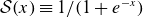
Momentum transfer cross-section from the refined model with $\chi$
(red dashed curve); Itikawa (Reference Itikawa1974) (green square marker); Buckman & Elford (Reference Buckman and Elford2000) (blue circle marker); and NIST standard database (Jablonski, Salvat & Powell Reference Jablonski, Salvat and Powell2004; Salvat, Jablonski & Powell Reference Salvat, Jablonski and Powell2005) (magenta bar).
$\chi$
(red dashed curve); Itikawa (Reference Itikawa1974) (green square marker); Buckman & Elford (Reference Buckman and Elford2000) (blue circle marker); and NIST standard database (Jablonski, Salvat & Powell Reference Jablonski, Salvat and Powell2004; Salvat, Jablonski & Powell Reference Salvat, Jablonski and Powell2005) (magenta bar).

To account for elastic scattering of low energy electrons due to collision with hydrogen neutrals, we borrow a function form from the Thomas–Fermi (TF) model (Breizman et al. Reference Breizman, Aleynikov, Hollmann and Lehnen2019) and refine it by fitting against experimental data (Itikawa Reference Itikawa1974; Buckman & Elford Reference Buckman and Elford2000; Jablonski et al. Reference Jablonski, Salvat and Powell2004; Salvat et al. Reference Salvat, Jablonski and Powell2005). The direct usage of the TF model is not rigorous because the TF model is valid for the partial screening effect of high-Z partially stripped ions/neutrals on energetic electrons: the majority of bound electrons need to have large principal quantum numbers and an incident electron should be energetic due to the first-order Born approximation (Landau & Lifshitz Reference Landau and Lifshitz2013; Hesslow et al. Reference Hesslow, Embréus, Hoppe, DuBois, Papp, Rahm and Fülöp2018).
According to Zhogolev & Konovalov (Reference Zhogolev and Konovalov2014) and Breizman et al. (Reference Breizman, Aleynikov, Hollmann and Lehnen2019), the function form of the elastic collision frequency is known as
 \begin{eqnarray} \nu _{el} = n_H c \frac {e^4}{4\pi \varepsilon _0^2 m^2 c^4} I_2 (y), \end{eqnarray}
where $I_2 (y)$
is the second screening coefficient with
$I_2 (y)$
is the second screening coefficient with $y=274p/mc$
. This coefficient grows logarithmically with
$y=274p/mc$
. This coefficient grows logarithmically with $y$
at the high-energy region, i.e.
$y$
at the high-energy region, i.e. $I_2(y) \approx I_2(y_*) + \ln (y/y_*)$
with
$I_2(y) \approx I_2(y_*) + \ln (y/y_*)$
with $y_*=26$
. We extrapolate this to the low-energy region, ensuring that
$y_*=26$
. We extrapolate this to the low-energy region, ensuring that $I_2$
approaches
$I_2$
approaches $0$
,
$0$
,
 \begin{equation} I_2(y) \approx I_2(y_*) + \frac {\ln \left [({y}/{y_*})^4 + \exp (-I_2(y_*))^4\right ]}{4} . \end{equation}
Let $\nu _{el}^{ref} \equiv \chi \nu _{el}$
be the refined frequency with a correction factor
$\nu _{el}^{ref} \equiv \chi \nu _{el}$
be the refined frequency with a correction factor $\chi$
. The outcome of refinement is displayed in figure 1 by fitting the momentum transfer (transport) cross-section
$\chi$
. The outcome of refinement is displayed in figure 1 by fitting the momentum transfer (transport) cross-section $\sigma _m^{el,eH} \approx \chi {{(e^4)}/{(4\pi \varepsilon _0^2 m_e^2 v^4)} }I_2$
to those of experimental data (Itikawa Reference Itikawa1974; Buckman & Elford Reference Buckman and Elford2000) and the NIST Standard Database (Jablonski et al. Reference Jablonski, Salvat and Powell2004; Salvat et al. Reference Salvat, Jablonski and Powell2005). The red curve goes to the magenta bars for high-energy particles while aligning well with experimental data at low energy range. In fact,
$\sigma _m^{el,eH} \approx \chi {{(e^4)}/{(4\pi \varepsilon _0^2 m_e^2 v^4)} }I_2$
to those of experimental data (Itikawa Reference Itikawa1974; Buckman & Elford Reference Buckman and Elford2000) and the NIST Standard Database (Jablonski et al. Reference Jablonski, Salvat and Powell2004; Salvat et al. Reference Salvat, Jablonski and Powell2005). The red curve goes to the magenta bars for high-energy particles while aligning well with experimental data at low energy range. In fact, $R^2\text{ score}$
is approximately
$R^2\text{ score}$
is approximately $0.999$
. The fitting finds
$0.999$
. The fitting finds
 \begin{equation} \chi = 1 + \frac {a^{el} (511\,000 (\gamma -1))^{b^{el}}}{1+c^{el} (511\,000 (\gamma -1))^{b^{el}}} ,\end{equation}
where $a^{el}=79.837201$
,
$a^{el}=79.837201$
, $b^{el}=-1.0992754$
and
$b^{el}=-1.0992754$
and $c^{el}=1.6387662$
.
$c^{el}=1.6387662$
.
2.2.2. Soft ionising collisions
Let the stopping power of soft ionising collisions on electrons have the logarithmic factor
 \begin{eqnarray} \bigg ( \frac {\text{d} \mathcal{E}}{\text{d}t} \bigg )_{\textit{iz}}^{\textit{soft}} = - \frac {n_H e^4}{4\pi \varepsilon _0^2 mv} \ln \varLambda _{\textit{iz}}^{\textit{soft}} . \end{eqnarray}
The stopping cross-section $\sigma _{\textit{iz}}^{\textit{sti}, \textit{soft}}(T)$
also measures the net effect of soft ionising collisions on energy loss,
$\sigma _{\textit{iz}}^{\textit{sti}, \textit{soft}}(T)$
also measures the net effect of soft ionising collisions on energy loss,
 \begin{equation} \sigma _{\textit{iz}}^{\textit{sti}, \textit{soft}}(T) = {\int} _0^{W_{\textit{bnd}}} (B+W) \frac {\text{d}\sigma _{\textit{iz}}(W, T)}{\text{d}W} \,\text{d}W, \end{equation}
where $W_{\textit{bnd}} = B w_{\textit{bnd}}$
. After straightforward calculation, for
$W_{\textit{bnd}} = B w_{\textit{bnd}}$
. After straightforward calculation, for $w_{\textit{bnd}}=ht-1$
,
$w_{\textit{bnd}}=ht-1$
,
 \begin{equation} \begin{split} \sigma _{\textit{iz}}^{\textit{sti}, \textit{soft}}(T) &= \frac {4\pi a_0^2 \alpha _{fs}^4 N}{(\beta _t^2 + \beta _u^2 + \beta _b^2)2b'} \Bigg\{ (f(ht-1) - f(0)) \Bigg[\ln \left(\frac {\beta _t^2}{1-\beta _t^2}\right) -\beta _t^2 - \ln (2b')\Bigg] \\ &\quad + \left(2-\frac {N_i}{N}\right)\Bigg[\frac {ht}{1+(1-h)t} -\frac {1}{t} + \ln \frac {1+(1-h)t}{t} \frac {1+2t'}{(1+t'/2)^2} + \ln ht \\ &\quad + \ln \frac {1+(1-h)t}{t} +\frac {b'^2}{(1+t'/2)^2}\frac {h^2t^2 - 1}{2}\Bigg] \Bigg\}, \end{split} \end{equation}
for $w_{\textit{bnd}} = {{(t-1)}/{2}}$
,
$w_{\textit{bnd}} = {{(t-1)}/{2}}$
,
 \begin{equation} \begin{split} \sigma _{\textit{iz}}^{\textit{sti}, \textit{soft}}(T) &= \frac {4\pi a_0^2 \alpha _{fs}^4 N}{(\beta _t^2 + \beta _u^2 + \beta _b^2)2b'}\Bigg\{ \Bigg(f\bigg(\frac {t-1}{2}\bigg) - f(0)) \Bigg[\ln \left(\frac {\beta _t^2}{1-\beta _t^2}\right) -\beta _t^2 - \ln (2b')\Bigg] \\ &\quad +\left(2-\frac {N_i}{N}\right)\Bigg[1-\frac {1}{t} + \ln \frac {t+1}{2t} \frac {1+2t'}{(1+t'/2)^2} + 2\ln \frac {t+1}{2} \\&\quad - \ln t +\frac {b'^2}{(1+t'/2)^2}\frac {t^2+2t-3}{8}\Bigg] \Bigg\} \end{split} \end{equation}
and for $w_{\textit{bnd}}=0$
,
$w_{\textit{bnd}}=0$
,
 \begin{equation} \begin{split} \sigma _{\textit{iz}}^{\textit{sti}, \textit{soft}}&(T) = 0, \end{split} \end{equation}
where $f(w) = {\int} \text{d}f/\text{d}w(w)\, \text{d}w = -b/(1+w) - c/(2(1+w)^2) - d/(3(1+w)^3) - e/$ $(4(1+w)^4)$
with
$(4(1+w)^4)$
with $b=-2.2473\boldsymbol{\times }10^{-2}$
,
$b=-2.2473\boldsymbol{\times }10^{-2}$
, $c=1.1775$
,
$c=1.1775$
, $d=-4.6264\boldsymbol{\times }10^{-1}$
and
$d=-4.6264\boldsymbol{\times }10^{-1}$
and $e=8.9064\boldsymbol{\times }10^{-2}$
listed in table I of Kim & Rudd (Reference Kim and Rudd1994).
$e=8.9064\boldsymbol{\times }10^{-2}$
listed in table I of Kim & Rudd (Reference Kim and Rudd1994).
The stopping power estimated from $\sigma _{\textit{iz}}^{\textit{sti}, \textit{soft}}(T)$
is
$\sigma _{\textit{iz}}^{\textit{sti}, \textit{soft}}(T)$
is
 \begin{eqnarray} \bigg ( \frac {\text{d} \mathcal{E}}{\text{d}t} \bigg )_{\textit{iz}}^{\textit{soft}} = - n_H v \sigma _{\textit{iz}}^{\textit{sti}, \textit{soft}} \equiv - \nu _{\textit{iz}}^{\textit{sti}, \textit{soft}} . \end{eqnarray}
Equating (2.27) and (2.32) yields
 \begin{eqnarray} \ln \varLambda _{\textit{iz}}^{\textit{soft}} = \frac {4 \pi \varepsilon _0^2 mv}{n_H e^4} \nu _{\textit{iz}}^{\textit{sti}, \textit{soft}}. \end{eqnarray}
2.2.3. Soft exciting collisions
Let the stopping power of soft exciting collisions on electrons have the logarithmic factor
 \begin{eqnarray} \bigg ( \frac {\text{d} \mathcal{E}}{\text{d}t} \bigg )_{ex}^{\textit{soft}} = - \frac {n_H e^4}{4\pi \varepsilon _0^2 mv} \ln \varLambda _{ex}^{\textit{soft}} . \end{eqnarray}
The stopping cross-section of soft exciting collision is $\sigma _{ex}^{ste,soft} = \sum _{n=2,10}\sigma _{ex}^{1n}E_{1n}$ $\mathcal{H}(T- ({E_{1n}}/{h}))$
due to fixed excitation energy. The stopping power estimated from
$\mathcal{H}(T- ({E_{1n}}/{h}))$
due to fixed excitation energy. The stopping power estimated from $\sigma _{ex}^{ste, soft}(T)$
is
$\sigma _{ex}^{ste, soft}(T)$
is
 \begin{eqnarray} \bigg ( \frac {\text{d} \mathcal{E}}{\text{d}t} \bigg )_{ex}^{\textit{soft}} = - n_H v \sigma _{ex}^{ste,soft} \equiv - \nu _{ex}^{ste, soft} . \end{eqnarray}
Equating (2.34) and (2.35) yields
 \begin{eqnarray} \ln \varLambda _{ex}^{\textit{soft}} = \frac {4 \pi \varepsilon _0^2 mv}{n_H e^4} \nu _{ex}^{ste, soft}. \end{eqnarray}
2.2.4. Logarithmic factor
The logarithm factor due to soft inelastic collisions is
 \begin{equation} \ln \varLambda ^{\textit{soft}} = \frac {4 \pi \varepsilon _0^2 mv}{n_H e^4} (\nu _{\textit{iz}}^{\textit{sti}, \textit{soft}} + \nu _{ex}^{ste, soft}) . \end{equation}
Remind that we deduce (2.37) by matching a function form of stopping power. That is to say, it does not originate from diverging nature of scattering cross-sections in small energy transfer limit like free–free Coulomb collisions (Rosenbluth et al. Reference Rosenbluth, MacDonald and Judd1957).
In the $h \to 1$
limit, all collisions are soft. The logarithmic factor due to total inelastic collisions can be obtained by taking this limit, i.e.
$h \to 1$
limit, all collisions are soft. The logarithmic factor due to total inelastic collisions can be obtained by taking this limit, i.e. $\ln \varLambda ^{tot} = \lim _{h\to 1} \ln \varLambda ^{\textit{soft}}$
, since the test particle operator in the FPB is approximated to the FP. The hard collision part becomes
$\ln \varLambda ^{tot} = \lim _{h\to 1} \ln \varLambda ^{\textit{soft}}$
, since the test particle operator in the FPB is approximated to the FP. The hard collision part becomes $\ln \varLambda ^{\textit{hard}} = \ln \varLambda ^{tot} - \ln \varLambda ^{\textit{soft}}$
.
$\ln \varLambda ^{\textit{hard}} = \ln \varLambda ^{tot} - \ln \varLambda ^{\textit{soft}}$
.
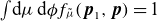
Logarithmic factor due to inelastic collisions, total (solid black), hard (blue dashed) and soft (red dash-dotted) with $h=0.1$
. Grey dotted line is the Bethe model extrapolated as a reference.
$h=0.1$
. Grey dotted line is the Bethe model extrapolated as a reference.

Figure 2 shows the smallness of the logarithmic factor for free-bound collisions. In fully ionised plasmas, the Coulomb logarithm measures the dominance of small angle scattering ( $\ln \varLambda \gg 1$
) and justifies neglect of higher order terms during derivation of the FP operator. In other words, such a system meets
$\ln \varLambda \gg 1$
) and justifies neglect of higher order terms during derivation of the FP operator. In other words, such a system meets $({\partial f}/{\partial t})_c \approx - \boldsymbol{\nabla } \boldsymbol{\cdot }(f \langle \Delta \boldsymbol{v} \rangle ) + {1}/{2} \boldsymbol{\nabla }\boldsymbol{\nabla } : (f \langle \Delta \boldsymbol{v} \Delta \boldsymbol{v} \rangle)$
since high-order terms like
$({\partial f}/{\partial t})_c \approx - \boldsymbol{\nabla } \boldsymbol{\cdot }(f \langle \Delta \boldsymbol{v} \rangle ) + {1}/{2} \boldsymbol{\nabla }\boldsymbol{\nabla } : (f \langle \Delta \boldsymbol{v} \Delta \boldsymbol{v} \rangle)$
since high-order terms like $\langle \Delta \boldsymbol{v} \Delta \boldsymbol{v} \Delta \boldsymbol{v} \rangle$
do not contain
$\langle \Delta \boldsymbol{v} \Delta \boldsymbol{v} \Delta \boldsymbol{v} \rangle$
do not contain $\ln \varLambda$
. For inelastic collisions, however, the logarithmic factor is so small that the assumption required for the expansion is broken. In addition, the inelastic collisions are predominantly hard for low-energy particles. Such collisions need to be accounted for by (2.23).
$\ln \varLambda$
. For inelastic collisions, however, the logarithmic factor is so small that the assumption required for the expansion is broken. In addition, the inelastic collisions are predominantly hard for low-energy particles. Such collisions need to be accounted for by (2.23).
2.2.5. Normalisation
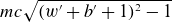
(a) Normalised deflection frequency and (b) slowing-down frequency as a function of incident electron energy. The legend of panel (a) is same as figure 1. Panel (b) is from the extrapolated Bethe model (Hesslow et al. Reference Hesslow, Embréus, Stahl, DuBois, Papp, Newton and Fülöp2017) (black solid), the FPB model in $h \rightarrow 1$
limit (red dashed) and with
$h \rightarrow 1$
limit (red dashed) and with $h=0.1$
(green dash-dotted).
$h=0.1$
(green dash-dotted). $n_e=10^{16} \ \text{m}^{-3}$
and
$n_e=10^{16} \ \text{m}^{-3}$
and $n_H=0.99 \boldsymbol{\cdot }10^{18} \ \text{m}^{-3}$
. Reprinted figure with permission from Lee et al. (Reference Lee, Aleynikov, De Vries, Kim, Lee, Hoppe, Park, Choi, Gwak and Na2024), copyright 2025 by the American Physical Society.
$n_H=0.99 \boldsymbol{\cdot }10^{18} \ \text{m}^{-3}$
. Reprinted figure with permission from Lee et al. (Reference Lee, Aleynikov, De Vries, Kim, Lee, Hoppe, Park, Choi, Gwak and Na2024), copyright 2025 by the American Physical Society.

Let $\tilde {\nu }_{\textit{iz}}^{\textit{sti}, \textit{soft}} = \nu _{\textit{iz}}^{\textit{sti}, \textit{soft}} \tau _c / mc^2$
,
$\tilde {\nu }_{\textit{iz}}^{\textit{sti}, \textit{soft}} = \nu _{\textit{iz}}^{\textit{sti}, \textit{soft}} \tau _c / mc^2$
, $\tilde {\nu }_{ex}^{ste, soft} = \nu _{ex}^{ste, soft} \tau _c / mc^2$
and
$\tilde {\nu }_{ex}^{ste, soft} = \nu _{ex}^{ste, soft} \tau _c / mc^2$
and $\ln \tilde {\varLambda }^{\textit{soft}} = n_H \ln \varLambda ^{\textit{soft}} /$ $ n_e \ln \varLambda$
. Neglecting the tilde, the normalised logarithmic factor due to inelastic collisions
$ n_e \ln \varLambda$
. Neglecting the tilde, the normalised logarithmic factor due to inelastic collisions $\ln \varLambda _{bound}$
is
$\ln \varLambda _{bound}$
is
 \begin{equation} \ln \varLambda ^{\textit{soft}} = \beta \big(\nu _{\textit{iz}}^{\textit{sti}, \textit{soft}} + \nu _{ex}^{ste, soft}\big). \end{equation}
For $\mathcal{C}_{FP}^{\textit{soft}} \{ f_e \}$
, we took a form given by Helander & Sigmar (Reference Helander and Sigmar2005). Using this form together with (2.25), (2.26) and (2.37),
$\mathcal{C}_{FP}^{\textit{soft}} \{ f_e \}$
, we took a form given by Helander & Sigmar (Reference Helander and Sigmar2005). Using this form together with (2.25), (2.26) and (2.37), $2\pi p^2 \mathcal{C}_{FP}^{\textit{soft}} \{ f_e \}$
becomes
$2\pi p^2 \mathcal{C}_{FP}^{\textit{soft}} \{ f_e \}$
becomes
 \begin{equation} 2\pi p^2 \mathcal{C}_{FP}^{\textit{soft}} \{ f_e \} = \frac {\partial }{\partial p} p \nu _S^{e,eb} F_e + \big(\nu _D^{e,eb} + \nu _D^{eH}\big) \mathcal{L}\{F_e\}, \end{equation}
where $\mathcal{L}$
is the Laplace operator (Helander & Sigmar Reference Helander and Sigmar2005) and characteristic collisional frequencies are
$\mathcal{L}$
is the Laplace operator (Helander & Sigmar Reference Helander and Sigmar2005) and characteristic collisional frequencies are
 \begin{align} \nu _S^{e,eb} &= \frac {\gamma ^2}{p^3} \ln \varLambda ^{\textit{soft}}, \end{align}
 \begin{align} \nu _D^{e,eb} &= \frac {\gamma }{p^3} \ln \varLambda ^{\textit{soft}}, \end{align}
 \begin{align} \nu _D^{eH} &= \frac {\gamma }{p^3} \chi \frac {n_H I_2^H(y)}{n_e \ln \varLambda }. \end{align}
Here, $\nu _D^{eH}$
and
$\nu _D^{eH}$
and $\nu _S^{e,eb}$
are shown in figures 3(a) and 3(b), respectively. All elastic collisions are accounted for by
$\nu _S^{e,eb}$
are shown in figures 3(a) and 3(b), respectively. All elastic collisions are accounted for by $\nu _D^{eH}$
in
$\nu _D^{eH}$
in $C_{FP}^{\textit{soft}}$
. For inelastic collisions of low-energy electrons, the soft collisions represent only a fraction of all collisions and the associated frequency is therefore lower. In the
$C_{FP}^{\textit{soft}}$
. For inelastic collisions of low-energy electrons, the soft collisions represent only a fraction of all collisions and the associated frequency is therefore lower. In the $h=0.1$
case, for instance,
$h=0.1$
case, for instance, $\nu _S^{e,eb}=0$
in
$\nu _S^{e,eb}=0$
in $\mathcal{C}^{eH}$
and
$\mathcal{C}^{eH}$
and $\mathcal{B}^{eH}$
treats all inelastic collisions below
$\mathcal{B}^{eH}$
treats all inelastic collisions below $102.043\,\text{eV}$
. This energy corresponds to
$102.043\,\text{eV}$
. This energy corresponds to $1/h$
of the minimal excitation energy for H. The ‘continuous’ soft collision energy loss is significantly reduced even above
$1/h$
of the minimal excitation energy for H. The ‘continuous’ soft collision energy loss is significantly reduced even above $102.043\,\text{eV}$
. Nevertheless, the green curve goes to the red curve for high-energy electrons due to the dominating soft collisions over the hard collisions.
$102.043\,\text{eV}$
. Nevertheless, the green curve goes to the red curve for high-energy electrons due to the dominating soft collisions over the hard collisions.
2.3. Invariance in $h$
$h$

The collision operator $\mathcal{C}^{eH}$
is invariant in the total particle source rate and total energy loss rate with respect to
$\mathcal{C}^{eH}$
is invariant in the total particle source rate and total energy loss rate with respect to $h$
, i.e.
$h$
, i.e. ${\partial }/{\partial h} [ {\int} \text{d}p \,\text{d}\mu 2\pi p^2 \ \mathcal{C} \{ f_e \} ] = {{\partial }/{\partial h}} [ {\int} \text{d}p\, \text{d}\mu \ (\gamma -1) 2\pi p^2 \mathcal{C} \{ f_e \} ] = 0$
. The invariance ensures the particle and energy conservation and, for a given distribution function, decouple an effect of energy loss allocation on electron acceleration from that of total energy loss.
${\partial }/{\partial h} [ {\int} \text{d}p \,\text{d}\mu 2\pi p^2 \ \mathcal{C} \{ f_e \} ] = {{\partial }/{\partial h}} [ {\int} \text{d}p\, \text{d}\mu \ (\gamma -1) 2\pi p^2 \mathcal{C} \{ f_e \} ] = 0$
. The invariance ensures the particle and energy conservation and, for a given distribution function, decouple an effect of energy loss allocation on electron acceleration from that of total energy loss.
2.3.1. Particle loss rate
Let us take an integral ${\int} \text{d}p \,\text{d}\mu$
on
${\int} \text{d}p \,\text{d}\mu$
on $2\pi p^2 \mathcal{C}^{eH} \{ f_e \}= 2\pi p^2 \mathcal{C}^{\textit{soft}}_{FP} \{ f_e \} + 2\pi p^2 \mathcal{B}^{\textit{hard}}_{\textit{iz}} \{ f_e \} + 2\pi p^2 \mathcal{B}^{\textit{hard}}_{ex} \{ f_e \}$
. The term
$2\pi p^2 \mathcal{C}^{eH} \{ f_e \}= 2\pi p^2 \mathcal{C}^{\textit{soft}}_{FP} \{ f_e \} + 2\pi p^2 \mathcal{B}^{\textit{hard}}_{\textit{iz}} \{ f_e \} + 2\pi p^2 \mathcal{B}^{\textit{hard}}_{ex} \{ f_e \}$
. The term ${\int} \text{d}p\, \text{d}\mu 2\pi p^2 \mathcal{C}^{\textit{soft}}_{FP} \{ f_e \}$
automatically goes to
${\int} \text{d}p\, \text{d}\mu 2\pi p^2 \mathcal{C}^{\textit{soft}}_{FP} \{ f_e \}$
automatically goes to $0$
due to its convective–diffusive form. An integral
$0$
due to its convective–diffusive form. An integral ${\int} \text{d}\mu$
on
${\int} \text{d}\mu$
on $2\pi p^2 \mathcal{B}^{\textit{hard}}_{\textit{iz}} \{ f_e \}$
yields
$2\pi p^2 \mathcal{B}^{\textit{hard}}_{\textit{iz}} \{ f_e \}$
yields
 \begin{align} {\int} \text{d}\mu 2\pi p^2 \mathcal{B}^{\textit{hard}}_{\textit{iz}} \{ f_e \} &= n_H mc^3 \tau _c \frac {p}{\gamma }\bigg [ {\int} _{\!\!p_{\textit{bnd}}} \text{d}p_1 \frac {\partial \sigma _{\textit{iz}}}{\partial W} \frac {p_1}{\gamma _1} F_e^0(p_1) \bigg ] - \nu _{\textit{iz}}^{\textit{hard}} F_e^0(p). \end{align}
For an integral ${\int} \text{d}p$
, change an integral variable from
${\int} \text{d}p$
, change an integral variable from $p$
to
$p$
to $W$
and swap the order of integration, i.e.
$W$
and swap the order of integration, i.e. ${\int} \text{d}p {\int} _{\!\!p_{\textit{bnd}}}\text{d}p_1 = {{1}/{(mc^2)}}{\int} \text{d}p_1 {\int} _0^{T-B-W_{\textit{bnd}}} \text{d}W$
. Then, an integral part
${\int} \text{d}p {\int} _{\!\!p_{\textit{bnd}}}\text{d}p_1 = {{1}/{(mc^2)}}{\int} \text{d}p_1 {\int} _0^{T-B-W_{\textit{bnd}}} \text{d}W$
. Then, an integral part ${\int} _0^{T-B-W_{\textit{bnd}}} \text{d}W {\partial \sigma _{\textit{iz}}^{\textit{hard}}}/{ \partial W} = \sigma _{\textit{iz}}+\sigma _{\textit{iz}}^{\textit{hard}}$
is isolated. The result of taking an integral
${\int} _0^{T-B-W_{\textit{bnd}}} \text{d}W {\partial \sigma _{\textit{iz}}^{\textit{hard}}}/{ \partial W} = \sigma _{\textit{iz}}+\sigma _{\textit{iz}}^{\textit{hard}}$
is isolated. The result of taking an integral ${\int} \text{d}p$
on (2.43) is independent of
${\int} \text{d}p$
on (2.43) is independent of $h$
, i.e.
$h$
, i.e.
 \begin{align} {\int} \text{d}p \,\text{d}\mu 2\pi p^2 \mathcal{B}^{\textit{hard}}_{\textit{iz}} \{ f_e \} &= {\int} \text{d}p_1 \ (\nu _{\textit{iz}} + \nu _{\textit{iz}}^{\textit{hard}}) F_e^0(p_1) - {\int} \text{d}p \ \nu _{\textit{iz}}^{\textit{hard}} F_e^0(p) \notag \\ &= {\int} \text{d}p \ \nu _{\textit{iz}} F_e^0(p). \end{align}
Using $\beta (p)\,\text{d}p = \beta (p^+_{1n})\,\text{d}p^+_{1n}$
, the excitation part is straightforward,
$\beta (p)\,\text{d}p = \beta (p^+_{1n})\,\text{d}p^+_{1n}$
, the excitation part is straightforward,
 \begin{align} {\int} \text{d}p \,\text{d}\mu 2\pi p^2 \mathcal{B}^{\textit{hard}}_{ex, 1s \to np} \{ f_e \} &= {\int} \text{d}p^+_{1n} \Big [ \nu _{ex,1s \to np}^{\textit{hard}}(p^+_{1n}) F_e^0(p^+_{1n}) \Big ] \notag \\ &\quad - {\int} \text{d}p \Big [ \nu _{ex,1s \to np}^{\textit{hard}}(p) F_e^0(p) \Big ] = 0. \end{align}
Finally, the outcome,
 \begin{equation} {\int} \text{d}p\, \text{d}\mu 2\pi p^2 \mathcal{C}^{eH} \{ f_e \}={\int} \text{d}p \ \nu _{\textit{iz}} F_e^0(p), \end{equation}
suggests the total particle loss is invariant in $h$
.
$h$
.
2.3.2. Energy loss rate
Take an integral ${\int} \text{d}p \,\text{d}\mu \gamma$
on
${\int} \text{d}p \,\text{d}\mu \gamma$
on $2\pi p^2 \mathcal{C}_{FP}^{\textit{soft}}$
and then the pitch angle scattering part automatically goes to
$2\pi p^2 \mathcal{C}_{FP}^{\textit{soft}}$
and then the pitch angle scattering part automatically goes to $0$
. The remaining part is
$0$
. The remaining part is
 \begin{align} {\int} \text{d}p \gamma \partial _p (p \nu _S^{e,eb} F_e^0(p)) &= {\int} \text{d}p \Big [\!-\nu _{\textit{iz}}^{\textit{sti}, \textit{soft}}(T) \Big ] F_e^0(p) + {\int} \text{d}p \Big [\!- \nu _{ex}^{ste,soft}(T) \Big ] F_e^0(p) . \end{align}
Take an integral ${\int} \text{d}\mu$
on the ionisation part in the Boltzmann operator to eliminate the scattering angle term,
${\int} \text{d}\mu$
on the ionisation part in the Boltzmann operator to eliminate the scattering angle term,
 \begin{align} {\int} \text{d}\mu 2\pi p^2 \mathcal{B}_{\textit{iz}}^{\textit{hard}} &= n_H mc^3 \tau _c \frac {p}{\gamma } {\int} _{\!\!p_{\textit{bnd}}} \text{d}p_1 \Big [\frac {\partial \sigma _{\textit{iz}}(W, T)}{\partial W} \frac {p_1}{\gamma _1} F_e^0 (p_1)\Big ] - \nu _{\textit{iz}}^{\textit{hard}} F_e^0 (p). \end{align}
For an integral ${\int} \gamma\, \text{d}p$
, change an integral variable from
${\int} \gamma\, \text{d}p$
, change an integral variable from $p$
to
$p$
to $W$
and swap the order of integration, i.e.
$W$
and swap the order of integration, i.e. ${\int} \text{d}p {\int} _{\!\!p_{\textit{bnd}}}\text{d}p_1 = {{1}/{(mc^2)}} {\int} \text{d}p_1 {\int} _0^{T-B-W_{\textit{bnd}}} \text{d}W$
. This isolates the integral of
${\int} \text{d}p {\int} _{\!\!p_{\textit{bnd}}}\text{d}p_1 = {{1}/{(mc^2)}} {\int} \text{d}p_1 {\int} _0^{T-B-W_{\textit{bnd}}} \text{d}W$
. This isolates the integral of ${\partial \sigma _{\textit{iz}}(W, T)}/{\partial W}$
. From
${\partial \sigma _{\textit{iz}}(W, T)}/{\partial W}$
. From $0$
to
$0$
to $(T-B)/2$
, the result of the integral is
$(T-B)/2$
, the result of the integral is ${\int} _{\!\!0}^{(T-B)/2} \text{d}W \gamma {\partial \sigma _{\textit{iz}}(W, T)}/{\partial W}= {1}/({mc^2})\sigma _{\textit{iz}}^{sti} + (1-b') \sigma _{\textit{iz}}$
. Then, take a variable transformation from
${\int} _{\!\!0}^{(T-B)/2} \text{d}W \gamma {\partial \sigma _{\textit{iz}}(W, T)}/{\partial W}= {1}/({mc^2})\sigma _{\textit{iz}}^{sti} + (1-b') \sigma _{\textit{iz}}$
. Then, take a variable transformation from $W$
to
$W$
to $T-B-\tilde {W}$
on the remaining part,
$T-B-\tilde {W}$
on the remaining part,
 \begin{align} {\int} _{\!\!0}^{T-B-W_{\textit{bnd}}} \text{d}W \gamma \frac {\partial \sigma _{\textit{iz}}(W, T)}{\partial W} &= \frac {1}{mc^2} \sigma _{\textit{iz}}^{sti} + (1-b') \sigma _{\textit{iz}} \notag \\ &\quad + {\int} _{\!\!W_{\textit{bnd}}}^{(T-B)/2} \text{d}\tilde {W} \gamma (T-B-\tilde {W}) \frac {\partial \sigma _{\textit{iz}}(\tilde {W}, T)}{\partial \tilde {W}}. \end{align}
The outcome of ${\int} \text{d}p \gamma$
on (2.48), resolving
${\int} \text{d}p \gamma$
on (2.48), resolving $\nu ^{\textit{hard}}_{\textit{iz}}= n_H c \tau _c {p}/{\gamma } {\int} _{\!\!W_{\textit{bnd}}}^{(T-B)/2}\text{d}\tilde {W} \partial \sigma _{\textit{iz}}$ ${(\tilde {W}, T)}/{\partial \tilde {W}}$
, becomes
${(\tilde {W}, T)}/{\partial \tilde {W}}$
, becomes
 \begin{align} \begin{split} {\int} {\text{d}\mu\,} \text{d}p \gamma 2\pi p^2 \mathcal{B}_{\textit{iz}}^{\textit{hard}} &= {\int} {\text{d}p_1} \Big [ \nu _{\textit{iz}}^{sti} + (1-b') \nu _{\textit{iz}} \Big ] F_e^0(p_1) + n_H c \tau _c {{\int} }{\text{d}p} \frac {p}{\gamma } F_e^0 (p) \\ &\quad \times \Bigg[{\int}{ _{W_{\textit{bnd}}}}^{(T-B)/2} d\tilde {W} (\gamma (T-B-\tilde {W}) - \gamma (T)) \frac {\partial \sigma _{\textit{iz}}(\tilde {W}, T)}{\partial \tilde {W}}\Bigg] \\ &= {\int} {\text{d}p} \Big [ \nu _{\textit{iz}}^{\textit{sti}, \textit{soft}} + (1-b') \nu _{\textit{iz}} \Big ] F_e^0(p) . \end{split} \end{align}
Take a ${\int}{\text{d}}\mu$
on the excitation part (
${\int}{\text{d}}\mu$
on the excitation part ( $1s \to np$
transition) in the Boltzmann operator,
$1s \to np$
transition) in the Boltzmann operator,
 \begin{align} {\int} \text{d}\mu 2\pi p^2 \mathcal{B}_{ex, 1s \to np}^{\textit{hard}} &= \nu _{ex, 1s \to np}^{\textit{hard}}(p^+_{1n}) \frac {\beta (p)}{\beta (p^+_{1n})} F_e^0 (p^+_{1n}) - \nu _{ex, 1s \to np}^{\textit{hard}}(p) F_e^0 (p). \end{align}
For ${\int} \text{d}p \gamma$
, use
${\int} \text{d}p \gamma$
, use $\beta (p^+_{1n})\,\text{d}p^+_{1n} = \beta (p)\, \text{d}p$
,
$\beta (p^+_{1n})\,\text{d}p^+_{1n} = \beta (p)\, \text{d}p$
,
 \begin{align} {\int} \text{d}\mu \,\text{d}p \gamma 2\pi p^2 \mathcal{B}_{ex, 1s \to np}^{\textit{hard}} &= {\int} \text{d}p^+_{1n}\gamma \Big [\nu _{ex, 1s \to np}^{\textit{hard}}(p^+_{1n}) F_e^0 (p^+_{1n})\Big ] \notag \\ &\quad - {\int} \text{d}p\gamma \Big [\nu _{ex, 1s \to np}^{\textit{hard}}(p) F_e^0 (p) \Big ] \notag \\ &= {\int} \text{d}p [(\gamma (T-E_{1n}) - \gamma (T)) ]\nu _{ex, 1s \to np}^{\textit{hard}} F_e^0 (p) \notag \\ &= {\int} \text{d}p \Big [ -\nu _{ex, 1s \to np}^{ste, hard} \Big ] F_e^0 (p). \end{align}
Finally, (2.46), (2.47), (2.50) and (2.52) yield the outcome,
 \begin{equation} {\int} \text{d}p \,\text{d}\mu (\gamma -1) 2\pi p^2 \mathcal{C}^{eH} \{ f_e \}={\int} \text{d}p \ \Big [\! - b'\nu _{\textit{iz}} - \nu _{ex}^{ste} \Big ] F_e^0(p), \end{equation}
which suggests the total energy loss is invariant in $h$
.
$h$
.
2.4. Collisions with free electrons and ions
We describe the kinetic model for collisions with free electrons and ions for completeness of this paper. The majority of free electrons are assumed a posteriori to be Maxwellian. The justification is essential for applying it to weakly ionised plasmas and will therefore be verified through numerical simulation in § 2.4.4.
The FP operator is used to account for the Coulomb collisions with free electrons and ions:
 \begin{equation} 2\pi p^2 \mathcal{C}_{FP} \{ f_e \} = 2\pi p^2 \mathcal{C}_{FP}^{e,i} \{ f_e \} + 2\pi p^2 \mathcal{C}_{FP}^{e,ef} \{ f_e \}. \end{equation}
The collisions with ions are described by the Lorentz operator (Helander & Sigmar Reference Helander and Sigmar2005):
 \begin{equation} 2\pi p^2 \mathcal{C}_{FP}^{e,i} \{ f_e \} = \nu _D^{ei} \mathcal{L}\{F_e\}. \end{equation}
The deflection frequency is
 \begin{equation} \nu _D^{ei} = \frac {\gamma }{p^3} \frac { \ln \varLambda _{\textit{free}} }{\ln \varLambda }. \end{equation}
We take $\ln \varLambda _{\textit{free}}$
from (29) of Breizman et al. (Reference Breizman, Aleynikov, Hollmann and Lehnen2019),
$\ln \varLambda _{\textit{free}}$
from (29) of Breizman et al. (Reference Breizman, Aleynikov, Hollmann and Lehnen2019),
 \begin{equation} \ln \varLambda _{free }= \frac {1}{2} \ln \frac {m^2c^2(\gamma ^2-1)(\gamma -1)}{2\hbar ^2 \omega _p^2 \gamma ^2}, \end{equation}
where $\omega _p \equiv \sqrt { {n_e e^2}/({m \varepsilon _0})}$
is the plasma frequency and
$\omega _p \equiv \sqrt { {n_e e^2}/({m \varepsilon _0})}$
is the plasma frequency and $\hbar$
is the Planck constant. While this form adequately describes a stopping power felt by energetic electrons from Coulomb collisions, it is unsuitable for cold electrons moving at speeds below the thermal velocity; it exhibits correct independence from electron temperature in the high-energy regime due to plasma wave excitation (Bohm & Gross Reference Bohm and Gross1949; Solodov & Betti Reference Solodov and Betti2008). Accordingly, an interpolation towards the Coulomb logarithm for thermal electrons, based on Richardson (Reference Richardson2019), was applied.
$\hbar$
is the Planck constant. While this form adequately describes a stopping power felt by energetic electrons from Coulomb collisions, it is unsuitable for cold electrons moving at speeds below the thermal velocity; it exhibits correct independence from electron temperature in the high-energy regime due to plasma wave excitation (Bohm & Gross Reference Bohm and Gross1949; Solodov & Betti Reference Solodov and Betti2008). Accordingly, an interpolation towards the Coulomb logarithm for thermal electrons, based on Richardson (Reference Richardson2019), was applied.
For collisions with free electrons, we linearise $\mathcal{C}_{FP}^{e,ef}$
because nonlinear terms are negligible:
$\mathcal{C}_{FP}^{e,ef}$
because nonlinear terms are negligible:
 \begin{equation} 2\pi p^2 \mathcal{C}_{FP}^{e,ef} \{ f_e \} \approx 2\pi p^2 \mathcal{C}_{FP}^{e,ef} \{ f_e, f_M \} + 2\pi p^2 \mathcal{C}_{FP}^{e,ef} \{ f_M, f_e \}, \end{equation}
where $f_M$
is the Maxwell distribution.
$f_M$
is the Maxwell distribution.
2.4.1. Test particle part
The test particle operator has a form given by Papp et al. (Reference Papp, Drevlak, Fülöp and Helander2011):
 \begin{equation} \begin{split} 2\pi p^2 \mathcal{C}_{FP} \{ f_e, f_M \} &= \frac {\partial }{\partial p} \bigg [ p \big(\nu _S^{e,ef} - \nu _\parallel ^{e,ef}\big) + \frac {1}{2} p^2 \nu _\parallel ^{e,ef} \frac {\partial }{\partial p} \bigg ] F_e + \big(\nu _D^{e,ef} + \nu _D^{ei}\big) \mathcal{L}\{F_e\} . \end{split} \end{equation}
This operator is suitable for arbitrary electron energies. The collision frequencies are
 \begin{align} \nu _S^{e,ef} &= \frac {G(X_G)}{\bar {T}_e p} \frac {\ln \varLambda _{\textit{free}}}{\ln \varLambda }, \end{align}
 \begin{align} \nu _\parallel ^{e,ef} &= 2\frac {\gamma }{p^3} G(X_G) \frac {\ln \varLambda _{\textit{free}}}{\ln \varLambda }, \end{align}
 \begin{align} \nu _D^{e,ef} &= \frac {\gamma }{p^3}(\varPhi (X_G) - G(X_G) + \bar {T}_e\beta ^2)\frac {\ln \varLambda _{\textit{free}}}{\ln \varLambda } , \end{align}
 \begin{align} \nu _D^{ei} &= \frac {\gamma }{p^3} \frac { \ln \varLambda _{\textit{free}} }{\ln \varLambda }, \end{align}
where $\bar {T}_e = T_e / mc^2$
,
$\bar {T}_e = T_e / mc^2$
, $X_G = v/v_{th}$
is the velocity normalised by the thermal velocity
$X_G = v/v_{th}$
is the velocity normalised by the thermal velocity $v_{th} = \sqrt {2 T_e / m}$
,
$v_{th} = \sqrt {2 T_e / m}$
, $G(X_G)$
is the Chandraseckhar function and
$G(X_G)$
is the Chandraseckhar function and $\varPhi (X_G)$
is the error function.
$\varPhi (X_G)$
is the error function.
2.4.2. Field particle part
The field particle operator is necessary to explicitly justify the background Maxwell assumption because the exponential factor is not negligible at the core.
The field particle operator has a form given by Li & Ernst (Reference Li and Ernst2011):
 \begin{equation} \begin{split} & 2\pi p^2 \mathcal{C} \{ f_M, f_e \} = \frac {1}{2\pi } {\int} \text{d}p' \,\text{d}\mu ' \left [\frac {1}{\beta _T^4} \left (\bigl(\beta ^2 + \beta '^2\bigr)\frac {4 K(\kappa )}{\lambda } - 2 \lambda E(\kappa )\right . \right . \\ & - \bigl(\beta ^2 - \beta '^2\bigr)^2\left . \left .\frac {2E(\kappa )}{\lambda ^3 (1-\kappa ^2)}\right ) -\frac {2}{\beta _T^2} \frac {4 K(\kappa )}{\lambda } \right ] \bar {F}_M(\boldsymbol{p}) F_e (\boldsymbol{p}') + \frac {2}{p^2} \bar {F}_M (\boldsymbol{p}) F_e (\boldsymbol{p}), \end{split} \end{equation}
where $\bar {F}_M = 2 \pi p^2 f_M / n_e$
,
$\bar {F}_M = 2 \pi p^2 f_M / n_e$
, $\beta _T = v_T/c$
,
$\beta _T = v_T/c$
, $\lambda ^2 = (\beta _\perp + \beta '_\perp )^2 + (\beta _\parallel - \beta '_\parallel )^2$
with
$\lambda ^2 = (\beta _\perp + \beta '_\perp )^2 + (\beta _\parallel - \beta '_\parallel )^2$
with $\beta _\perp = \beta \sqrt {1-\mu ^2}$
and
$\beta _\perp = \beta \sqrt {1-\mu ^2}$
and $\beta _\parallel = \beta \mu$
, and
$\beta _\parallel = \beta \mu$
, and $\kappa ^2 = 4 \beta _\perp \beta '_\perp / \lambda ^2$
. Here,
$\kappa ^2 = 4 \beta _\perp \beta '_\perp / \lambda ^2$
. Here, $K$
and
$K$
and $E$
are the complete elliptic integral of the first and second kinds, respectively.
$E$
are the complete elliptic integral of the first and second kinds, respectively.
2.4.3. Conservation laws
The conservation laws are approximately satisfied with the free–free collision operator (2.58). The relativistic operator that was matched to obtain (2.59) (Papp et al. Reference Papp, Drevlak, Fülöp and Helander2011) originates from the Beliaev–Budker kernel (Beliaev & Budker Reference Beliaev and Budker1956; Landau et al. Reference Landau, Lifshitz and Pitaevskij1981) by taking the Taylor expansion up to the second order (Sandquist et al. Reference Sandquist, Sharapov, Helander and Lisak2006). However, the only correction given by this matching from the semi-relativistic operator (Helander & Sigmar Reference Helander and Sigmar2005) is the $\bar {T}_e \beta ^2$
term in (2.62) that is much smaller than
$\bar {T}_e \beta ^2$
term in (2.62) that is much smaller than $\varPhi (X_G) \to 1$
for energetic electrons due to
$\varPhi (X_G) \to 1$
for energetic electrons due to $\bar {T}_e \ll 1$
. Therefore, both operators can be represented by the Landau kernel (Landau et al. Reference Landau, Lifshitz and Pitaevskij1981) and conservation laws are approximately satisfied (Landau et al. Reference Landau, Lifshitz and Pitaevskij1981) in cold weakly ionised plasmas. Note that the Landau kernel is indeed semi-relativistic and appropriate if one of the colliding particles is non-relativistic (Braams & Karney Reference Braams and Karney1987).
$\bar {T}_e \ll 1$
. Therefore, both operators can be represented by the Landau kernel (Landau et al. Reference Landau, Lifshitz and Pitaevskij1981) and conservation laws are approximately satisfied (Landau et al. Reference Landau, Lifshitz and Pitaevskij1981) in cold weakly ionised plasmas. Note that the Landau kernel is indeed semi-relativistic and appropriate if one of the colliding particles is non-relativistic (Braams & Karney Reference Braams and Karney1987).
2.4.4. Verification of the Maxwellian assumption
The ‘core’ Maxwell assumption can be guaranteed if $n_e \ln \varLambda _{\textit{free}} \gg n_H \ln \varLambda _{bound}$
, where
$n_e \ln \varLambda _{\textit{free}} \gg n_H \ln \varLambda _{bound}$
, where $\ln \varLambda _{\textit{free}}$
is the Coulomb logarithm for free–free collisions and
$\ln \varLambda _{\textit{free}}$
is the Coulomb logarithm for free–free collisions and $\ln \varLambda _{bound}$
is the logarithmic factor for free–bound collisions. This condition is evidently satisfied below
$\ln \varLambda _{bound}$
is the logarithmic factor for free–bound collisions. This condition is evidently satisfied below $100\,\text{eV}$
because
$100\,\text{eV}$
because $\ln \varLambda _{bound}$
felt by a majority of electrons is
$\ln \varLambda _{bound}$
felt by a majority of electrons is $\ln \varLambda ^{\textit{soft}}$
and thus is vanishingly small (see red curve in figure 2). Therefore, the lower energy part of the population is predominantly Maxwellian. The argument is only true for the background electron distribution, not for the entire electron distribution.
$\ln \varLambda ^{\textit{soft}}$
and thus is vanishingly small (see red curve in figure 2). Therefore, the lower energy part of the population is predominantly Maxwellian. The argument is only true for the background electron distribution, not for the entire electron distribution.
The adequacy of the background Maxwellian assumption is numerically verified by confirming whether the Maxwell distribution function is sustained or not under the effect of free-bound collisions accounted by $\mathcal{C}$
. The numerical simulation is carried out by initiating
$\mathcal{C}$
. The numerical simulation is carried out by initiating $F_M$
and then evolving it for 20 μs under the weakly ionised condition where the ionisation fraction
$F_M$
and then evolving it for 20 μs under the weakly ionised condition where the ionisation fraction $\alpha \equiv {n_e}/({n_H + n_e}) = 1\,\%$
. Figure 4 shows resulting
$\alpha \equiv {n_e}/({n_H + n_e}) = 1\,\%$
. Figure 4 shows resulting $F_e^0$
. The black curve aligns well with the red curve. This good agreement indicates inelastic collisions do not distort
$F_e^0$
. The black curve aligns well with the red curve. This good agreement indicates inelastic collisions do not distort $F_e^0$
as severely as violate the Maxwell assumption. In this specific example, a total friction of free–bound collision dominates free–free collision due to
$F_e^0$
as severely as violate the Maxwell assumption. In this specific example, a total friction of free–bound collision dominates free–free collision due to $n_e \ln \varLambda _{\textit{free}} \ll n_H \ln \varLambda ^{tot}$
. Nonetheless, the Maxwell assumption is valid because the majority of electrons do not experience inelastic collisions at all, i.e.
$n_e \ln \varLambda _{\textit{free}} \ll n_H \ln \varLambda ^{tot}$
. Nonetheless, the Maxwell assumption is valid because the majority of electrons do not experience inelastic collisions at all, i.e. $n_e \ln \varLambda _{\textit{free}} \gg n_H \ln \varLambda ^{\textit{soft}}$
. Indeed, free–bound collisions are strong, as seen by the blue curve, which clearly deviates from Maxwellian due to the misuse of the FP operator. For the verification, the ionising avalanche is regulated by adopting the test particle part in
$n_e \ln \varLambda _{\textit{free}} \gg n_H \ln \varLambda ^{\textit{soft}}$
. Indeed, free–bound collisions are strong, as seen by the blue curve, which clearly deviates from Maxwellian due to the misuse of the FP operator. For the verification, the ionising avalanche is regulated by adopting the test particle part in $\mathcal{C}^{eH}$
, while the field particle part is included in
$\mathcal{C}^{eH}$
, while the field particle part is included in $\mathcal{C}_{FP}$
for the low energy population. The detailed description for the implementation is in § 3.
$\mathcal{C}_{FP}$
for the low energy population. The detailed description for the implementation is in § 3.
Maxwell distribution function (black solid curve) and $F_e^0$
that evolves for 20 μs from the black curve with the FPB (red dashed curve, h = 0.1) and FP (blue dotted curve, h = 0.99) operators.
$F_e^0$
that evolves for 20 μs from the black curve with the FPB (red dashed curve, h = 0.1) and FP (blue dotted curve, h = 0.99) operators. $(n_H + n_e) = 10^{18} \ \text{m}^{-3}$
,
$(n_H + n_e) = 10^{18} \ \text{m}^{-3}$
, $T_e = 1\,\text{eV}$
and
$T_e = 1\,\text{eV}$
and $\alpha = 1\,\%$
.
$\alpha = 1\,\%$
.

2.5. Non-diffusive electron acceleration mechanism
The free–free and free–bound interactions exhibit significantly different interaction distances. This difference distinguishes the electron acceleration mechanisms. For free–free collisions, all electrons feel the interactions due to the long-range nature in the single particle description. In the kinetic description, electrons with the same energy have the same slowing down frequency. The FP operator takes into account disparities in the momentum exchanges using the velocity space diffusion frequency. Through the diffusion mechanism within the narrow singular layer across the critical momentum in phase space, the upward Dreicer flow can form under the effect of electric field, below which the mean frictional force exceeds the electric force. In contrast, the range of interaction is short for free–bound inelastic collisions due to a screened charge of neutrals in the single particle description. Therefore, some electrons can accelerate freely without undergoing inelastic collisions whenever they encounter a neutral particle. In the kinetic description, this mechanism is evidently distinct from the diffusive process and occurs over the electrons’ acceleration trajectories in the low-energy region of phase space, where most inelastic collisions are hard so should be described by the Boltzmann operator; electrons can share the slowing down frequency only if the associated energy transfer is very small compared with their energy, i.e. for soft collisions.
Mean frictional force considered by the FP operator as a function of incident electron energy. Free–bound collisions are from the extrapolated Bethe model (Hesslow et al. Reference Hesslow, Embréus, Stahl, DuBois, Papp, Newton and Fülöp2017) (black dashed dotted curve), the FPB model in $h \rightarrow 1$
limit, same to the FP model (blue solid curve), and with
$h \rightarrow 1$
limit, same to the FP model (blue solid curve), and with $h=0.1$
(red dashed curve). Green dotted curve is the electric force.
$h=0.1$
(red dashed curve). Green dotted curve is the electric force. $n_e + n_H =10^{18} \ \text{m}^{-3}$
,
$n_e + n_H =10^{18} \ \text{m}^{-3}$
, $E=0.2 \ \text{Vm}^{-1}$
,
$E=0.2 \ \text{Vm}^{-1}$
, $T_e = 5\,\text{eV}$
and
$T_e = 5\,\text{eV}$
and $\ln \varLambda _{\textit{free}} = 15$
.
$\ln \varLambda _{\textit{free}} = 15$
. $\alpha = 1\,\%, \ 2\,\%, \ 5\,\%$
and
$\alpha = 1\,\%, \ 2\,\%, \ 5\,\%$
and $11\,\%$
for panels (a), (b), (c) and (d), respectively.
$11\,\%$
for panels (a), (b), (c) and (d), respectively.

Such accounting of binary nature of inelastic collisions dramatically changes the critical energy crossing for free acceleration. This is clarified in figure 5 that shows mean frictional forces considered by the FP operator for the ionisation fractions $\alpha =1\,\%, \ 2\,\%, \ 5\,\%$
and
$\alpha =1\,\%, \ 2\,\%, \ 5\,\%$
and $11 \,\%$
. The corresponding parameters are close to that of standard Ohmic discharge in KSTAR tokamak (Yoo et al. Reference Yoo2018; Lee et al. Reference Lee2023a
) and ITER plasma initiation (de Vries & Gribov Reference de Vries and Gribov2019). Note that the mean frictional force is shared by electrons with the same energy through the slowing down frequency in each model. Other collisions considered by the binary Boltzmann operator are excluded in this computation. If the FP operator describes all collisions (blue or black curve), electron runaway begins at the critical energy crossing (e.g. see blue circle in figure 5
a). However, the FPB treatment can eliminate the crossing as shown in figure 5(a) if the ionisation fraction is sufficiently low. In this case, the Dreicer condition (Dreicer Reference Dreicer1959) is completely satisfied for some electrons: all electrons that do not experience hard inelastic collisions are runaway. Even in less extreme cases, the proposed model significantly modifies the critical energy by an order of magnitude (figure 5
b) or allows the virtual free acceleration (figure 5
c). The increased ionisation fraction makes the change in the critical energy less significant. Yet, the frictional force can be notably reduced even in this case (figure 5
d). In summary, the proposed model captures the non-diffusive Dreicer mechanism and allows for variations in the critical energy beyond the mean-friction approximation. Another noteworthy aspect is the associated diffusion with soft inelastic collisions, which will be addressed in a future study.
$11 \,\%$
. The corresponding parameters are close to that of standard Ohmic discharge in KSTAR tokamak (Yoo et al. Reference Yoo2018; Lee et al. Reference Lee2023a
) and ITER plasma initiation (de Vries & Gribov Reference de Vries and Gribov2019). Note that the mean frictional force is shared by electrons with the same energy through the slowing down frequency in each model. Other collisions considered by the binary Boltzmann operator are excluded in this computation. If the FP operator describes all collisions (blue or black curve), electron runaway begins at the critical energy crossing (e.g. see blue circle in figure 5
a). However, the FPB treatment can eliminate the crossing as shown in figure 5(a) if the ionisation fraction is sufficiently low. In this case, the Dreicer condition (Dreicer Reference Dreicer1959) is completely satisfied for some electrons: all electrons that do not experience hard inelastic collisions are runaway. Even in less extreme cases, the proposed model significantly modifies the critical energy by an order of magnitude (figure 5
b) or allows the virtual free acceleration (figure 5
c). The increased ionisation fraction makes the change in the critical energy less significant. Yet, the frictional force can be notably reduced even in this case (figure 5
d). In summary, the proposed model captures the non-diffusive Dreicer mechanism and allows for variations in the critical energy beyond the mean-friction approximation. Another noteworthy aspect is the associated diffusion with soft inelastic collisions, which will be addressed in a future study.
3. Numerical implementation
We implement the FPB operator in the self-consistent kinetic simulation (Aleynikov & Breizman Reference Aleynikov and Breizman2017) using FiPy, a finite volume partial differential equation (PDE) solver (Guyer, Wheeler & Warren Reference Guyer, Wheeler and Warren2009). In FiPy, the discretisation of $\mathcal{B}^{\textit{hard}} \{ F_e \}$
should be given in a volume-averaged form to ensure the particle conservation by
$\mathcal{B}^{\textit{hard}} \{ F_e \}$
should be given in a volume-averaged form to ensure the particle conservation by
 \begin{equation} {\int} _{\!\!p_{l,i}}^{p_{r,i}} \text{d}p {\int} _{\!\!\mu _{l,j}}^{\mu _{r,j}} \text{d}\mu \mathcal{B}^{\textit{hard}} \{ F_e \} \approx \mathcal{B}^{\textit{hard}} \{ F_e \} (p_i, \mu _{\!j}) \Delta p_i \Delta \mu _{\!j}, \end{equation}
where $(p_i, \mu _{\!j})$
is the (i, j)th cell centred coordinate,
$(p_i, \mu _{\!j})$
is the (i, j)th cell centred coordinate, $l$
and
$l$
and $r$
denote the left and right side cell face, respectively,
$r$
denote the left and right side cell face, respectively, $\Delta p_i = p_{r,i}-p_{l,i}$
, and
$\Delta p_i = p_{r,i}-p_{l,i}$
, and $\Delta \mu _{\!j} = \mu _{r,j}-\mu _{l,j}$
.
$\Delta \mu _{\!j} = \mu _{r,j}-\mu _{l,j}$
.
3.1. Discretisation of
$\mathcal{B}^{\textit{hard}}_{\textit{iz}} \{ F_e \}$

In the integral term in (2.23), $(p_1,\mu _1)$
and
$(p_1,\mu _1)$
and $(p, \mu )$
denote the continuous phase-space coordinates of electrons before and after collisions, respectively. During the numerical discretisation, these coordinates are replaced with
$(p, \mu )$
denote the continuous phase-space coordinates of electrons before and after collisions, respectively. During the numerical discretisation, these coordinates are replaced with $(p_k,\mu _{l'})$
for incident electrons, and
$(p_k,\mu _{l'})$
for incident electrons, and $(p_i,\mu _{\!j})$
for scattered and ejected electrons. A complete analytic integration is only possible in the
$(p_i,\mu _{\!j})$
for scattered and ejected electrons. A complete analytic integration is only possible in the $(p_i,\mu _{\!j})$
-coordinate because
$(p_i,\mu _{\!j})$
-coordinate because $F_e(p_k, \mu _{l'})$
is discretised. Hence, after discretising
$F_e(p_k, \mu _{l'})$
is discretised. Hence, after discretising $\mathcal{B}^{\textit{hard}}_{\textit{iz}} \{ F_e \}$
in the
$\mathcal{B}^{\textit{hard}}_{\textit{iz}} \{ F_e \}$
in the $(p_i,\mu _{\!j})$
-coordinate and erasing the dependence on
$(p_i,\mu _{\!j})$
-coordinate and erasing the dependence on $p_i$
and
$p_i$
and $\mu _{\!j}$
through summation, we will find a proper discretisation of the
$\mu _{\!j}$
through summation, we will find a proper discretisation of the $(p_k,\mu _{l'})$
-coordinate required for the particle conservation.
$(p_k,\mu _{l'})$
-coordinate required for the particle conservation.
Consider taking an integral ${\int} _{\!\!\mu _{l,j}}^{\mu _{r,j}} \text{d}\mu$
on
${\int} _{\!\!\mu _{l,j}}^{\mu _{r,j}} \text{d}\mu$
on $\mathcal{B}^{\textit{hard}}_{\textit{iz}} \{ F_e \}$
and discretise the
$\mathcal{B}^{\textit{hard}}_{\textit{iz}} \{ F_e \}$
and discretise the $\mu$
-integral using the relation,
$\mu$
-integral using the relation,
 \begin{align} &{\int} _{\!\!\mu _{l,j}}^{\mu _{r,j}} \text{d}\mu \frac {\mathcal{H}((1-\mu ^2)(1-\mu _1^2)-(\mu ^*-\mu \mu _1)^2)}{\sqrt {(1-\mu ^2)(1-\mu _1^2)-(\mu ^*-\mu \mu _1)^2}} \notag\\&\quad = \sin ^{-1} \bigg [ \min _2 \bigg (-1, \frac {\mu _{r,j} - \mu _1 \mu ^*}{\sqrt {(1-\mu _1^2)(1-\mu ^{*2})}}, 1 \bigg ) \bigg ] \notag \\ &\qquad - \sin ^{-1} \bigg [ \min _2 \bigg (-1, \frac {\mu _{l,j} - \mu _1 \mu ^*}{\sqrt {(1-\mu _1^2)(1-\mu ^{*2})}}, 1 \bigg ) \bigg ]. \end{align}
Here, $\sum _{\!j}$
erases the
$\sum _{\!j}$
erases the $\mu _{\!j}$
-dependence owing to
$\mu _{\!j}$
-dependence owing to $\mu _{l,0}=-1$
and
$\mu _{l,0}=-1$
and $\mu _{r,-1}=1$
with the particle conservation, where the index
$\mu _{r,-1}=1$
with the particle conservation, where the index $-1$
indicates the last one. Subsequently, discretise the
$-1$
indicates the last one. Subsequently, discretise the $p$
-integral by taking
$p$
-integral by taking ${\int} _{\!\!p_{l,i}}^{p_{r,i}} \text{d}p$
on
${\int} _{\!\!p_{l,i}}^{p_{r,i}} \text{d}p$
on $\sum _{\!j} {\int} _{\!\!\mu _{l,j}}^{\mu _{r,j}} \text{d}\mu \mathcal{B}^{\textit{hard}}_{\textit{iz}} \{ F_e \}$
and using the relation,
$\sum _{\!j} {\int} _{\!\!\mu _{l,j}}^{\mu _{r,j}} \text{d}\mu \mathcal{B}^{\textit{hard}}_{\textit{iz}} \{ F_e \}$
and using the relation,
 \begin{align} {\int} _{\!\!p_{l,i}}^{p_{r,i}} \text{d}p &\bigg [ mc^2 \frac {p}{\gamma } \frac {\partial \sigma _{\textit{iz}}(W,T)}{\partial W} \bigg ] = \Delta \sigma _{\textit{iz}}(w_{r,i}, T) - \Delta \sigma _{\textit{iz}}(w_{l,i}, T), \end{align}
where $w_{r,i}= (\sqrt {p_{r,i}^2+1}-1)/b'$
,
$w_{r,i}= (\sqrt {p_{r,i}^2+1}-1)/b'$
, $w_{l,i}= (\sqrt {p_{l,i}^2+1}-1)/b'$
and
$w_{l,i}= (\sqrt {p_{l,i}^2+1}-1)/b'$
and $\Delta \sigma _{\textit{iz}}(w,T)$
is
$\Delta \sigma _{\textit{iz}}(w,T)$
is
 \begin{align} \Delta \sigma _{\textit{iz}}(w,T) &\equiv {\int} _{\!\!0}^{w}\text{d}w \frac {\partial \sigma _{\textit{iz}}(W, T)}{\partial W}\notag\\& = \frac {4\pi a_0^2 \alpha _{fs}^4 N}{(\beta _t^2 + \beta _u^2 + \beta _b^2)2b'} \Bigg\{ \bar {D}(0, w)\Bigg [\ln \left(\frac {\beta _t^2}{1-\beta _t^2}\right) -\beta _t^2 - \ln (2b') \Bigg] \notag \\ &\quad + \left(2-\frac {N_i}{N}\right) \Bigg [1 - \frac {1}{t} + \frac {1}{t-w} -\frac {1}{w+1} \notag \\ &\quad -\ln \left((w+1)\frac {t}{t-w}\right)\frac {1}{t+1} \frac {1+2t'}{(1+t'/2)^2} +\frac {{b\prime }^2}{(1+t'/2)^2}w\Bigg] \Bigg\}. \end{align}
Here,
 \begin{align*}\bar {D}(0, w) &= \frac {1}{N} {\int} _{\!\!0}^{w}\frac {1}{1+w}\frac {\text{d}f}{\text{d}w}\,\text{d}w = \frac {b}{2}\left[1-\frac {1}{(1+w)^2}\right] + \frac {c}{3}\left[1-\frac {1}{(1+w)^3}\right] \notag\\&\quad + \frac {d}{4}\left[1-\frac {1}{(1+w)^4}\right] + \frac {e}{5}\left[1-\frac {1}{(1+w)^5}\right]\!.\end{align*}
Swapping the order of integration with $p_1$
,
$p_1$
, $\sum _i$
erases the
$\sum _i$
erases the $p_i$
-dependence:
$p_i$
-dependence:
 \begin{align} &\sum _i {\int} _{\!\!p_{pnd}} \text{d}p_1\, \text{d}\mu _1 \Big [ \Delta \sigma _{\textit{iz}}(w_{r,i}, T) - \Delta \sigma _{\textit{iz}}(w_{l,i}, T) \Big ] \notag \\ &\quad = {\int} \text{d}p_1 \,\text{d}\mu _1 \sum _{i\lt i^*} \Big [ \Delta \sigma _{\textit{iz}}(w_{r,i}, T) - \Delta \sigma _{\textit{iz}}(w_{l,i}, T) \Big ] \notag \\ &\quad= {\int} \text{d}p_1 \text{d}\mu _1 \Big [ \sigma _{\textit{iz}}(T) + \sigma _{\textit{iz}}^{\textit{hard}}(T) \Big ], \end{align}
where we replace $\Delta \sigma _{\textit{iz}}(w_{l,0}, T)$
with
$\Delta \sigma _{\textit{iz}}(w_{l,0}, T)$
with $\Delta \sigma _{\textit{iz}}(0, T)$
,
$\Delta \sigma _{\textit{iz}}(0, T)$
, $\Delta \sigma _{\textit{iz}}(w_{r,i^*}, T)$
with
$\Delta \sigma _{\textit{iz}}(w_{r,i^*}, T)$
with $\Delta \sigma _{\textit{iz}}(t-w_{\textit{bnd}}-1, T)$
, and
$\Delta \sigma _{\textit{iz}}(t-w_{\textit{bnd}}-1, T)$
, and $i^*$
satisfies
$i^*$
satisfies $w_{l,i^*}\lt t-w_{\textit{bnd}}-1$
and
$w_{l,i^*}\lt t-w_{\textit{bnd}}-1$
and $w_{l,i^*+1}\geqslant t-w_{\textit{bnd}}-1$
. Then, the ionisation part reduces to
$w_{l,i^*+1}\geqslant t-w_{\textit{bnd}}-1$
. Then, the ionisation part reduces to
 \begin{align} &\sum _{i,j} {\int} _{\!\!p_{l,i}}^{p_{r,i}} \text{d}p {\int} _{\!\!\mu _{l,j}}^{\mu _{r,j}} \text{d}\mu \mathcal{B}^{\textit{hard}}_{\textit{iz}} \{ F_e \} \notag \\ &\quad = \sum _{k,l'} {\int} _{\!\!p_{l,k}}^{p_{r,k}} {\int} _{\!\!\mu _{l,l'}}^{\mu _{r,l'}} \Big [(\nu _{\textit{iz}}(T_k)+\nu _{\textit{iz}}^{\textit{hard}}(T_k)) F_e (p_k, \mu _{l'})\Big ]\, \text{d}p_k\, \text{d}\mu _{l'} \notag \\ &\qquad - \sum _{i,j} {\int} _{\!\!p_{l,i}}^{p_{r,i}} {\int} _{\!\!\mu _{l,j}}^{\mu _{r,j}} \Big [\nu _{\textit{iz}}^{\textit{hard}}(T_i)) F_e (p_i, \mu _{\!j})\Big ]\, \text{d}p_i\, \text{d}\mu _{\!j}. \end{align}
We discretise ${\int} _{\!\!p_{l,k}}^{p_{r,k}} \text{d}p_k [\nu _{\textit{iz}}(T_k)+\nu _{\textit{iz}}^{\textit{hard}}(T_k)) F_e (p_k, \mu _{l'})]$
grounded in the fact that
${\int} _{\!\!p_{l,k}}^{p_{r,k}} \text{d}p_k [\nu _{\textit{iz}}(T_k)+\nu _{\textit{iz}}^{\textit{hard}}(T_k)) F_e (p_k, \mu _{l'})]$
grounded in the fact that $F_e(p_k,\mu _{l'})$
shows the exponential dependence on
$F_e(p_k,\mu _{l'})$
shows the exponential dependence on $p_k$
, and both of
$p_k$
, and both of $\nu _{\textit{iz}}(T_k)$
and
$\nu _{\textit{iz}}(T_k)$
and $\nu _{\textit{iz}}^{\textit{hard}}(T_k)$
have the algebraic dependence on
$\nu _{\textit{iz}}^{\textit{hard}}(T_k)$
have the algebraic dependence on $p_k$
, i.e.
$p_k$
, i.e. $|\partial _p \ln (F_e)| \gg |\partial _p \ln (\nu _{\textit{iz}})|$
and
$|\partial _p \ln (F_e)| \gg |\partial _p \ln (\nu _{\textit{iz}})|$
and $|\partial _p \ln (F_e)| \gg |\partial _p \ln (\nu _{\textit{iz}}^{\textit{hard}})|$
:
$|\partial _p \ln (F_e)| \gg |\partial _p \ln (\nu _{\textit{iz}}^{\textit{hard}})|$
:
 \begin{align} {\int} _{\!\!p_{l,k}}^{p_{r,k}} \text{d}p_k \nu _{\textit{iz}}(T_k) F_e (p_k, \mu _{l'}) &\approx \nu _{\textit{iz}}(T_k) F_e (p_k, \mu _{l'}) \Delta p_k, \end{align}
 \begin{align} {\int} _{\!\!p_{l,k}}^{p_{r,k}} \text{d}p_k \nu _{\textit{iz}}^{\textit{hard}}(T_k) F_e (p_k, \mu _{l'}) &\approx \nu _{\textit{iz}}^{\textit{hard}}(T_k) F_e (p_k, \mu _{l'}) \Delta p_k. \end{align}
An exception where the condition $|\partial _p \ln (F_e)| \gg |\partial _p \ln (\nu _{\textit{iz}})|$
can be severely broken and influence the discretisation is nearby
$|\partial _p \ln (F_e)| \gg |\partial _p \ln (\nu _{\textit{iz}})|$
can be severely broken and influence the discretisation is nearby $T \approx B$
due to onset of ionising collisions. We replace
$T \approx B$
due to onset of ionising collisions. We replace $\Delta p_{k^*}=p_{r,k^*}-p_{l,k^*}$
in (3.7) and (3.8) with
$\Delta p_{k^*}=p_{r,k^*}-p_{l,k^*}$
in (3.7) and (3.8) with $\Delta p_{k^*}=p_{r,k^*}-\sqrt {(b'+1)^2-1}$
, where
$\Delta p_{k^*}=p_{r,k^*}-\sqrt {(b'+1)^2-1}$
, where $k^*$
satisfies
$k^*$
satisfies $T_{r,k^*} \gt B$
and
$T_{r,k^*} \gt B$
and $T_{l,k^*} \lt B$
. The remaining
$T_{l,k^*} \lt B$
. The remaining $\mu _{l'}$
part is straightforward:
$\mu _{l'}$
part is straightforward: ${\int} _{\!\!\mu _{l,l'}}^{\mu _{r,l'}} \text{d}\mu _{l'} F_e(p_k,\mu _{l'}) = F_e(p,\mu _{l'}) \Delta \mu _{l'}$
. Finally, the fully discretised form of
${\int} _{\!\!\mu _{l,l'}}^{\mu _{r,l'}} \text{d}\mu _{l'} F_e(p_k,\mu _{l'}) = F_e(p,\mu _{l'}) \Delta \mu _{l'}$
. Finally, the fully discretised form of $\mathcal{B}^{\textit{hard}}_{\textit{iz}} \{ F_e \}$
is
$\mathcal{B}^{\textit{hard}}_{\textit{iz}} \{ F_e \}$
is
 \begin{align} \mathcal{B}^{\textit{hard}}_{\textit{iz}} \{ F_e \} (p_i, \mu _{\!j}) = \sum _{k,l'} \bigl[\mathcal{B}^{\textit{hard}}_{\textit{iz}} &\{ F_e \} (p_i, \mu _{\!j})\bigr]_{k,l'}\Delta p_k \Delta \mu _{l'} - \nu _{\textit{iz}}^{\textit{hard}}(p_i) F_e(p_i, \mu _{\!j}), \end{align}
where
 \begin{align} &[\mathcal{B}^{\textit{hard}}_{\textit{iz}} \{ F_e \} (p_i, \mu _{\!j})]_{k,l'} = \frac {1}{\Delta p_i \Delta \mu _{\!j}} \Bigg [ \Bigg \{ \frac {1}{\pi } \Bigg ( \sin ^{-1}\Bigg [\min _2 \bigg(-1, \frac {\mu _{r,j}-\mu _1 \mu ^*}{\sqrt {(1-\mu _1^2)(1-\mu ^{*2})}},1\Bigg) \Bigg] \notag \\ &\quad - \sin ^{-1} \Bigg [\min _2 \Bigg (-1, \frac {\mu _{l,j}-\mu _1 \mu ^*}{\sqrt {(1-\mu _1^2)(1-\mu ^{*2})}},1\Bigg) \Bigg ] \Bigg ) - \frac {\Delta \mu _{\!j}}{2} \Bigg \} \frac {1}{1+\frac {0.1}{p_i}} + \frac {\Delta \mu _{\!j}}{2}\Bigg ] \notag \\ &\quad \times \Big ( \Delta \nu _{\textit{iz}} (w_{r,i}, T_k) - \Delta \nu _{\textit{iz}} (w_{l, i}, T_k) \Big ) F_e(p_k, \mu _{l'}) \end{align}
and $\Delta \nu _{\textit{iz}} = n_H c \tau _c \Delta \sigma _{\textit{iz}} (w_i, T_k) \beta _k$
.
$\Delta \nu _{\textit{iz}} = n_H c \tau _c \Delta \sigma _{\textit{iz}} (w_i, T_k) \beta _k$
.
3.2. Discretisation of
$\mathcal{B}^{\textit{hard}}_{ex} \{ F_e \}$

Consider ${\int} _{\!\!p_{l,i}}^{p_{r,i}} \text{d}p$
on the source term of
${\int} _{\!\!p_{l,i}}^{p_{r,i}} \text{d}p$
on the source term of $\mathcal{B}^{\textit{hard}}_{ex, 1s \to np} \{ F_e \}$
and discretise the
$\mathcal{B}^{\textit{hard}}_{ex, 1s \to np} \{ F_e \}$
and discretise the $p$
-integral,
$p$
-integral,
 \begin{align} &{\int} _{\!\!p_{l,i}}^{p_{r,i}} \text{d}p_i \frac {\nu _{ex, 1s \to np}^{\textit{hard}}(p^+_{1n})}{2} \frac {\beta (p_i)}{\beta (p^+_{1n})} F_e^0(p^+_{1n}) \notag \\ &\quad= \sum _k {\int} _{\!\!p_{l,i}}^{p_{r,i}} \text{d}p_i {\int} _{\!\!p_{l,k}}^{p_{r,k}} \text{d}p_k \Bigg [ \frac {\nu _{ex, 1s \to np}^{\textit{hard}}(p_k)}{2} \frac {\beta (p_i)}{\beta (p_k)} F_e^0(p_k) \frac {\text{d}T_k}{\text{d}p_k} \delta (T_k - W_i - E_{1n}) \Bigg ] \notag \\ &\quad= \sum _k {\int} _{\!\!p_{l,k}}^{p_{r,k}} \text{d}p_k \Bigg [ \frac {\nu _{ex, 1s \to np}^{\textit{hard}}(p_k)}{2} F_e^0(p_k) \Bigg ] \Bigg [ {\int} _{\!\!W_{l,i}}^{W_{r,i}} \text{d}W_i \delta (T_k - W_i - E_{1n}) \Bigg ] \end{align}
Here, we use the integral representation as the first step and interchange the order of integration as the second step. Suppose we just take ${\int} _{\!\!W_{l,i}}^{W_{r,i}} \text{d}W_i \delta(T_k - W_i -$ $ E_{1n}) = 1$
. In that case, the particle conservation is adequate but the ith cell-centred energy
$ E_{1n}) = 1$
. In that case, the particle conservation is adequate but the ith cell-centred energy $W_i$
is not equal to
$W_i$
is not equal to $T_k-E_{1n}$
. To overcome this drawback,
$T_k-E_{1n}$
. To overcome this drawback, $\delta (T_k - W_i - E_{1n})$
is smoothed as meeting
$\delta (T_k - W_i - E_{1n})$
is smoothed as meeting
 \begin{align} \Delta \hat {W}^{1n}_{i-1,k} + \Delta \hat {W}^{1n}_{i,k} + \Delta \hat {W}^{1n}_{i+1,k} &= 1, \end{align}
 \begin{align} \Delta \hat {W}^{1n}_{i-1,k} W_{i-1} + \Delta \hat {W}^{1n}_{i,k} W_{i} + \Delta \hat {W}^{1n}_{i+1,k} W_{i+1} &= T_k + E_{1n}, \end{align}
where $\Delta \hat {W}^{1n}_{i,k} \equiv {\int} _{\!\!W_{l,i}}^{W_{r,i}} \text{d}W_i \hat {\delta } (T_k - W_i - E_{1n})$
and
$\Delta \hat {W}^{1n}_{i,k} \equiv {\int} _{\!\!W_{l,i}}^{W_{r,i}} \text{d}W_i \hat {\delta } (T_k - W_i - E_{1n})$
and $\hat {\delta }$
is the smoothed Dirac-delta function. If
$\hat {\delta }$
is the smoothed Dirac-delta function. If $W_{l,i} \lt T_k-E_{1n} \lt W_i$
, set
$W_{l,i} \lt T_k-E_{1n} \lt W_i$
, set $\Delta \hat {W}^{1n}_{i+1,k} = 0$
and then,
$\Delta \hat {W}^{1n}_{i+1,k} = 0$
and then,
 \begin{align} \Delta \hat {W}^{1n}_{i-1,k} = \frac {W_i - T_k + E_{1n}}{W_i - W_{i-1}},\Delta \hat {W}^{1n}_{i,k} = \frac {T_k - E_{1n} -W_{i-1}}{W_i - W_{i-1}}. \end{align}
If $W_{i} \lt T_k-E_{1n} \lt W_{r,i}$
, set
$W_{i} \lt T_k-E_{1n} \lt W_{r,i}$
, set $\Delta \hat {W}^{1n}_{i-1,k} = 0$
and then,
$\Delta \hat {W}^{1n}_{i-1,k} = 0$
and then,
 \begin{align} \Delta \hat {W}^{1n}_{i,k} = \frac {W_{i+1} - T_k + E_{1n}}{W_{i+1} - W_{i}},\Delta \hat {W}^{1n}_{i+1,k} = \frac {T_k - E_{1n} -W_{i}}{W_{i+1} - W_{i}}. \end{align}
If $0 \lt T_k-E_{1n} \lt W_{l,0}$
, just set
$0 \lt T_k-E_{1n} \lt W_{l,0}$
, just set $\Delta \hat {W}^{1n}_{0,k} = 1$
, assuming the energy loss due to this approximation is negligible. After skipping the trivial
$\Delta \hat {W}^{1n}_{0,k} = 1$
, assuming the energy loss due to this approximation is negligible. After skipping the trivial $\mu$
-discretisation, we take
$\mu$
-discretisation, we take $\sum _i$
to erase the
$\sum _i$
to erase the $i$
-dependence. Then,
$i$
-dependence. Then,
 \begin{align} \sum _{i,j} {\int} _{\!\!p_{l,i}}^{p_{r,i}} \text{d}p_i {\int} _{\!\!\mu _{l,j}}^{\mu _{r,j}} \text{d}\mu _{\!j} \mathcal{B}^{\textit{hard}}_{ex, 1s \to np} \{ F_e \} &= \sum _k {\int} _{\!\!p_{l,k}}^{p_{r,k}} \text{d}p_k \Big [ \nu _{ex, 1s \to np}^{\textit{hard}}(p_k) F_e^0(p_k) \Big ] \notag \\&\quad - \sum _i {\int} _{\!\!p_{l,i}}^{p_{r,i}} \text{d}p_i \Big [ \nu _{ex, 1s \to np}^{\textit{hard}}(p_i) F_e^0(p_i) \Big ]. \end{align}
We discretise ${\int} _{\!\!p_{l,k}}^{p_{r,k}} \text{d}p_k [\nu _{ex,1n \to np}^{\textit{hard}}(p_k) F_e^0 (p_k)]$
similarly to (3.8),
${\int} _{\!\!p_{l,k}}^{p_{r,k}} \text{d}p_k [\nu _{ex,1n \to np}^{\textit{hard}}(p_k) F_e^0 (p_k)]$
similarly to (3.8),
 \begin{equation} {\int} _{\!\!p_{l,k}}^{p_{r,k}} \text{d}p_k \nu _{ex, 1s \to np}^{\textit{hard}}(p_k) F_e^0 (p_k) \approx \nu _{ex, 1s \to np}^{\textit{hard}}(p_k) F_e^0 (p_k) \Delta p_k. \end{equation}
There are two exceptions that we replace: $\Delta p_{k^*}=p_{r,k^*}-p_{l,k^*}$
in (3.17) with
$\Delta p_{k^*}=p_{r,k^*}-p_{l,k^*}$
in (3.17) with $\Delta p_{k^*}=p_{r,k^*}-\sqrt {(E_{1n}'+1)^2-1}$
, where
$\Delta p_{k^*}=p_{r,k^*}-\sqrt {(E_{1n}'+1)^2-1}$
, where $k^*$
satisfies
$k^*$
satisfies $T_{r,k^*} \gt E_{1n}$
and
$T_{r,k^*} \gt E_{1n}$
and $T_{l,k^*} \lt E_{1n}$
, and
$T_{l,k^*} \lt E_{1n}$
, and $\Delta p_{k^{**}}=p_{r,k^{**}}-p_{l,k^{**}}$
with
$\Delta p_{k^{**}}=p_{r,k^{**}}-p_{l,k^{**}}$
with $\Delta p_{k^{**}}=\sqrt {({{E_{1n}'}/{h}}+1)^2-1}-p_{l,k^{**}}$
, where
$\Delta p_{k^{**}}=\sqrt {({{E_{1n}'}/{h}}+1)^2-1}-p_{l,k^{**}}$
, where $k^{**}$
satisfies
$k^{**}$
satisfies $T_{r,k^{**}} \gt {{(E_{1n})}/{h}}$
and
$T_{r,k^{**}} \gt {{(E_{1n})}/{h}}$
and $T_{l,k^{**}} \lt {({E_{1n})}/{h}}$
. Finally, the fully discretised form of
$T_{l,k^{**}} \lt {({E_{1n})}/{h}}$
. Finally, the fully discretised form of $\mathcal{B}^{\textit{hard}}_{ex} \{ F_e \}$
is
$\mathcal{B}^{\textit{hard}}_{ex} \{ F_e \}$
is
 \begin{align} [\mathcal{B}^{\textit{hard}}_{ex} \{ F_e \}(p_i, \mu _{\!j})]_k &= \sum _n \left [ \frac {\Delta p_k}{\Delta p_i} \frac {\nu _{ex, 1s \to np}^{\textit{hard}}}{2} F_e^0(p_k) \Delta \hat {W}_{i,k}^{1n} - \nu _{ex, 1s\to np}^{\textit{hard}}(p_i) F_e(p_i, \mu _{\!j}) \right ]\!. \end{align}
4. Non-diffusive Dreicer generation in weakly ionised plasmas
In this section, we select an appropriate value of $h$
as the ratio of the characteristic excitation energy to the critical runaway energy of interest, i.e.
$h$
as the ratio of the characteristic excitation energy to the critical runaway energy of interest, i.e. ${\sim} 0.1$
(Lee et al. Reference Lee, Aleynikov, De Vries, Kim, Lee, Hoppe, Park, Choi, Gwak and Na2024), to account for the binary nature using the Boltzmann operator (2.23).
${\sim} 0.1$
(Lee et al. Reference Lee, Aleynikov, De Vries, Kim, Lee, Hoppe, Park, Choi, Gwak and Na2024), to account for the binary nature using the Boltzmann operator (2.23).
Steady-state solutions of $F_e^0$
with the FP (red dashed curve, h = 0.1) and FPB (blue solid curve, h = 0.99) operators.
$F_e^0$
with the FP (red dashed curve, h = 0.1) and FPB (blue solid curve, h = 0.99) operators. $(n_H + n_e) = 10^{18} \ \text{m}^{-3}$
,
$(n_H + n_e) = 10^{18} \ \text{m}^{-3}$
, $T_e = 5\,\text{eV}$
and
$T_e = 5\,\text{eV}$
and $E=0.2 \ \text{Vm}^{-1}$
.
$E=0.2 \ \text{Vm}^{-1}$
. $\alpha = 1\,\%, \ 2\,\%, \ 5\,\%$
and
$\alpha = 1\,\%, \ 2\,\%, \ 5\,\%$
and $11\,\%$
for panels (a), (b), (c) and (d), respectively. (a) Reprinted figure with permission from Lee et al. (Reference Lee, Aleynikov, De Vries, Kim, Lee, Hoppe, Park, Choi, Gwak and Na2024), copyright 2025 by the American Physical Society.
$11\,\%$
for panels (a), (b), (c) and (d), respectively. (a) Reprinted figure with permission from Lee et al. (Reference Lee, Aleynikov, De Vries, Kim, Lee, Hoppe, Park, Choi, Gwak and Na2024), copyright 2025 by the American Physical Society.

The non-diffusive electron acceleration mechanism that was discussed in § 2.5 is demonstrated in figure 6, where the steady-state solutions are illustrated for various ionisation fractions (corresponding to figure 5). For the demonstration, we only took the test particle part to eliminate the runaway avalanche effect (Rosenbluth & Putvinski Reference Rosenbluth and Putvinski1997) by setting upper boundary of integral in (2.23) to $\sqrt {(2w+b'+2)(2w+b')}$
. Blue curves in figure 6(a–d) represent the solutions where most collisions are described with the FP operator (h = 0.99). In all cases, the resulting
$\sqrt {(2w+b'+2)(2w+b')}$
. Blue curves in figure 6(a–d) represent the solutions where most collisions are described with the FP operator (h = 0.99). In all cases, the resulting $F_e^0 \lt 10^{3} \text{m}^{-3}$
with electron energy above
$F_e^0 \lt 10^{3} \text{m}^{-3}$
with electron energy above $1 \ \text{keV}$
. Indeed, no Dreicer flow is expected in such conditions according to effectiveness of the Dreicer generation (Jayakumar, Fleischmann & Zweben Reference Jayakumar, Fleischmann and Zweben1993)
$1 \ \text{keV}$
. Indeed, no Dreicer flow is expected in such conditions according to effectiveness of the Dreicer generation (Jayakumar, Fleischmann & Zweben Reference Jayakumar, Fleischmann and Zweben1993) $E/E_d^{\textit{eff}} \lt 0.02$
with
$E/E_d^{\textit{eff}} \lt 0.02$
with $E_d^{\textit{eff}} \equiv ({e^3 (n_e \ln \varLambda _{\textit{free}} + n_H \ln \varLambda _{bound})}/{4 \pi \varepsilon _0^2 T_e})$
, where an effect of free-bound collisions are considered by replacing
$E_d^{\textit{eff}} \equiv ({e^3 (n_e \ln \varLambda _{\textit{free}} + n_H \ln \varLambda _{bound})}/{4 \pi \varepsilon _0^2 T_e})$
, where an effect of free-bound collisions are considered by replacing $n_e \ln \varLambda _{\textit{free}}$
as
$n_e \ln \varLambda _{\textit{free}}$
as $n_e \ln \varLambda _{\textit{free}} + n_H \ln \varLambda _{bound}$
(Martín-Solís et al. Reference Martín-Solís, Loarte and Lehnen2015) and
$n_e \ln \varLambda _{\textit{free}} + n_H \ln \varLambda _{bound}$
(Martín-Solís et al. Reference Martín-Solís, Loarte and Lehnen2015) and $\ln \varLambda _{bound} \approx \ln \varLambda ^{tot} \approx 5$
(see figure 2). The red dashed curve shows the solution with the FPB collision operator with
$\ln \varLambda _{bound} \approx \ln \varLambda ^{tot} \approx 5$
(see figure 2). The red dashed curve shows the solution with the FPB collision operator with $h=0.1$
. This solution is close to the Maxwellian in lower energy where free–free collisions dominate. However, it differs significantly at higher energy where the binary Boltzmann collisions allow for virtually free acceleration for some particles. These freely accelerated particles become runaways. The more
$h=0.1$
. This solution is close to the Maxwellian in lower energy where free–free collisions dominate. However, it differs significantly at higher energy where the binary Boltzmann collisions allow for virtually free acceleration for some particles. These freely accelerated particles become runaways. The more $\alpha$
is, the less REs are created since continuous free–free collisions induce stronger frictions than free–bound collisions.
$\alpha$
is, the less REs are created since continuous free–free collisions induce stronger frictions than free–bound collisions.
Dreicer generation rate as a function of $\alpha$
: with the FP (blue square,
$\alpha$
: with the FP (blue square, $h=0.99$
) and FPB (red circle,
$h=0.99$
) and FPB (red circle, $h=0.1$
) operators, and the analytic formula of Connor & Hastie (Reference Connor and Hastie1975). In the legend,
$h=0.1$
) operators, and the analytic formula of Connor & Hastie (Reference Connor and Hastie1975). In the legend, $\ln \varLambda$
is the Coulomb logarithm for free electrons
$\ln \varLambda$
is the Coulomb logarithm for free electrons $\ln \varLambda _{\textit{free}}$
and
$\ln \varLambda _{\textit{free}}$
and $\ln \varLambda _b$
is the logarithmic factor for bound electrons
$\ln \varLambda _b$
is the logarithmic factor for bound electrons $\ln \varLambda _{bound}$
. For instance,
$\ln \varLambda _{bound}$
. For instance, $\ln \varLambda _{\textit{free}} = 18$
and
$\ln \varLambda _{\textit{free}} = 18$
and $\ln \varLambda _{bound} = 0$
for the green solid curve, and
$\ln \varLambda _{bound} = 0$
for the green solid curve, and $\ln \varLambda _{\textit{free}} = 18$
and
$\ln \varLambda _{\textit{free}} = 18$
and $\ln \varLambda _{bound} = 5$
for the magenta dashed curve, required for collisional frequency computation. Here,
$\ln \varLambda _{bound} = 5$
for the magenta dashed curve, required for collisional frequency computation. Here, $(n_H + n_e) = 10^{18} \ \text{m}^{-3}$
,
$(n_H + n_e) = 10^{18} \ \text{m}^{-3}$
, $T_e = 5\,\text{eV}$
and
$T_e = 5\,\text{eV}$
and $E=0.2 \, \text{V m}^{-1}$
. Error bars are estimated by scanning
$E=0.2 \, \text{V m}^{-1}$
. Error bars are estimated by scanning $E=0.18\, \text{V m}^{-1}$
to
$E=0.18\, \text{V m}^{-1}$
to $E=0.22$
(
$E=0.22$
( $\pm 10\, \%$
). Reprinted figure with permission from Lee et al. (Reference Lee, Aleynikov, De Vries, Kim, Lee, Hoppe, Park, Choi, Gwak and Na2024), copyright 2025 by the American Physical Society.
$\pm 10\, \%$
). Reprinted figure with permission from Lee et al. (Reference Lee, Aleynikov, De Vries, Kim, Lee, Hoppe, Park, Choi, Gwak and Na2024), copyright 2025 by the American Physical Society.

Figure 7 shows the Dreicer generation rate as a function of the ionisation fraction. In this case, the binary nature of collisions plays a critical role in RE generation as indicated by the condition $E/E_d \gt 0.025$
, but
$E/E_d \gt 0.025$
, but $E/E_d^{\textit{eff}} \lt 0.02$
: the conventional Dreicer generation is ineffective for these parameters, while the Dreicer generation accounted by Boltzmann operator is effective and results in
$E/E_d^{\textit{eff}} \lt 0.02$
: the conventional Dreicer generation is ineffective for these parameters, while the Dreicer generation accounted by Boltzmann operator is effective and results in $10^{13} \ \text{m}^{-3} \text{s}^{-1}$
for
$10^{13} \ \text{m}^{-3} \text{s}^{-1}$
for $\alpha = 0.01$
. This is consistent with the analytical indicator of effectiveness since
$\alpha = 0.01$
. This is consistent with the analytical indicator of effectiveness since $E/E_d \approx 0.43 \gg 0.02$
, but
$E/E_d \approx 0.43 \gg 0.02$
, but $E/E_d^{\textit{eff}} \approx 0.015$
. The observed rates are much lower than the analytic prediction by Connor & Hastie (Reference Connor and Hastie1975) without free–bound collisions (green curve in figure 7). Our numerical FP calculations for the Dreicer generation (blue squares) consider inelastic slowing-down and thereby agree with the Connor–Hastie formula if
$E/E_d^{\textit{eff}} \approx 0.015$
. The observed rates are much lower than the analytic prediction by Connor & Hastie (Reference Connor and Hastie1975) without free–bound collisions (green curve in figure 7). Our numerical FP calculations for the Dreicer generation (blue squares) consider inelastic slowing-down and thereby agree with the Connor–Hastie formula if $E_d^{\textit{eff}}$
with
$E_d^{\textit{eff}}$
with $\ln \varLambda _{bound} \approx 5$
deduced from
$\ln \varLambda _{bound} \approx 5$
deduced from $\ln \varLambda ^{tot}$
is used in the formula (dashed curve).
$\ln \varLambda ^{tot}$
is used in the formula (dashed curve).
5. Conclusion
The collision operator for electrons in cold weakly ionised plasmas is developed to analyse the electron runaway process. The FPB operator for free–bound collisions is derived with the help of valid collision cross-sections for elastic (Itikawa Reference Itikawa1974; Buckman & Elford Reference Buckman and Elford2000; Jablonski et al. Reference Jablonski, Salvat and Powell2004; Salvat et al. Reference Salvat, Jablonski and Powell2005; Breizman et al. Reference Breizman, Aleynikov, Hollmann and Lehnen2019) and inelastic collisions (Kim & Rudd Reference Kim and Rudd1994; Kim et al. Reference Kim, Santos and Parente2000; Kim Reference Kim2001). The operator is invariant in particle and energy loss of electrons with respect to $h$
since the integral boundary defining the logarithmic factor is appropriately selected (Embréus et al. Reference Embréus, Stahl and Fülöp2018), which in turn ensures the particle and energy conservation. For free–free collisions, the validity of the linearised collision operator with sufficiently low ionisation fraction (
$h$
since the integral boundary defining the logarithmic factor is appropriately selected (Embréus et al. Reference Embréus, Stahl and Fülöp2018), which in turn ensures the particle and energy conservation. For free–free collisions, the validity of the linearised collision operator with sufficiently low ionisation fraction ( $\sim$
middle phase of breakdown (Yoo et al. Reference Yoo, Lee, Kim and Na2017, Reference Yoo2018; Yoo & Na Reference Yoo and Na2022) or early burn-through (Kim et al. Reference Kim2012)) is verified by elucidating that the Maxwell distribution function can be sustained under the strong effect of neutrals.
$\sim$
middle phase of breakdown (Yoo et al. Reference Yoo, Lee, Kim and Na2017, Reference Yoo2018; Yoo & Na Reference Yoo and Na2022) or early burn-through (Kim et al. Reference Kim2012)) is verified by elucidating that the Maxwell distribution function can be sustained under the strong effect of neutrals.
For numerical simulations, we present the complete analytic expression for the volume averaged form of the FPB operator. This can be implemented in the FVM-based numerical solver such as FiPy (Guyer et al. Reference Guyer, Wheeler and Warren2009).
Employing the FPB operator, we generalise the Dreicer generation model for weakly ionised plasmas to the non-diffusive regimes. An essential role of the binary nature of inelastic collisions is played in the Dreicer generation. Therefore, this work is envisaged to provide the precise RE generation rate for designing a runaway-free reactor start-up.
One of the promising applications of this work is to couple the kinetic model to ‘fluid’ plasma burn-through simulation (Kim et al. Reference Kim2012, Reference Kim2022) like fluid-kinetic disruption RE simulation (Aleynikov & Breizman Reference Aleynikov and Breizman2017; Hoppe, Embreus & Fülöp Reference Hoppe, Embreus and Fülöp2021). This coupling will facilitate a self-consistent simulation of runaway current evolution as well as a fully kinetic description of the ionising avalanche. Moreover, the electron cyclotron pre-ionisation (Lloyd et al. Reference Lloyd, Jackson, Taylor, Lazarus, Luce and Prater1991) will be investigated at a kinetic level by coupling this with nonlinear electron-cyclotron energy gain model (Suvorov & Tokman Reference Suvorov and Tokman1988; Farina & Pozzoli Reference Farina and Pozzoli1991; Farina, Pozzoli & Romé Reference Farina, Pozzoli and Romé1991; Seol, Hegna & Callen Reference Seol, Hegna and Callen2009; Farina Reference Farina2018; Johansson & Aleynikov Reference Johansson and Aleynikov2024; Gwak et al. Reference Gwak, Yoo, Kim, Lee, Lee and Na2025).
Acknowledgements
Y.L. is grateful for fruitful discussions with Dr Hyun-Tae Kim, Dr Jeongwon Lee, Professor Mathias Hoppe, Mr Jinwoo Gwak and Professor Gyungjin Choi. The views and opinions expressed herein do not necessarily reflect those of the ITER Organization.
Editor Tünde Fülöp thanks the referees for their advice in evaluating this article.
Funding
This research was supported by National R&D Program through the National Research Foundation of Korea (NRF) funded by Ministry of Science and ICT (2021M3F7A1084419). This research was supported by the National Research Foundation of Korea (NRF) grant funded by the Korean Government (MSIT) (RS-2024-00409564). This research was supported by R&D Program of ‘Optimal Basic Design of DEMO Fusion Reactor, CN2502-1’ through the Korea Institute of Fusion Energy (KFE) funded by the Government funds. The authors also gratefully acknowledge The Research Institute of Energy and Resources, The Institute of Engineering Research and the SNU Energy Initiative at Seoul National University.
Declaration of interests
The authors declare no conflicts of interest.

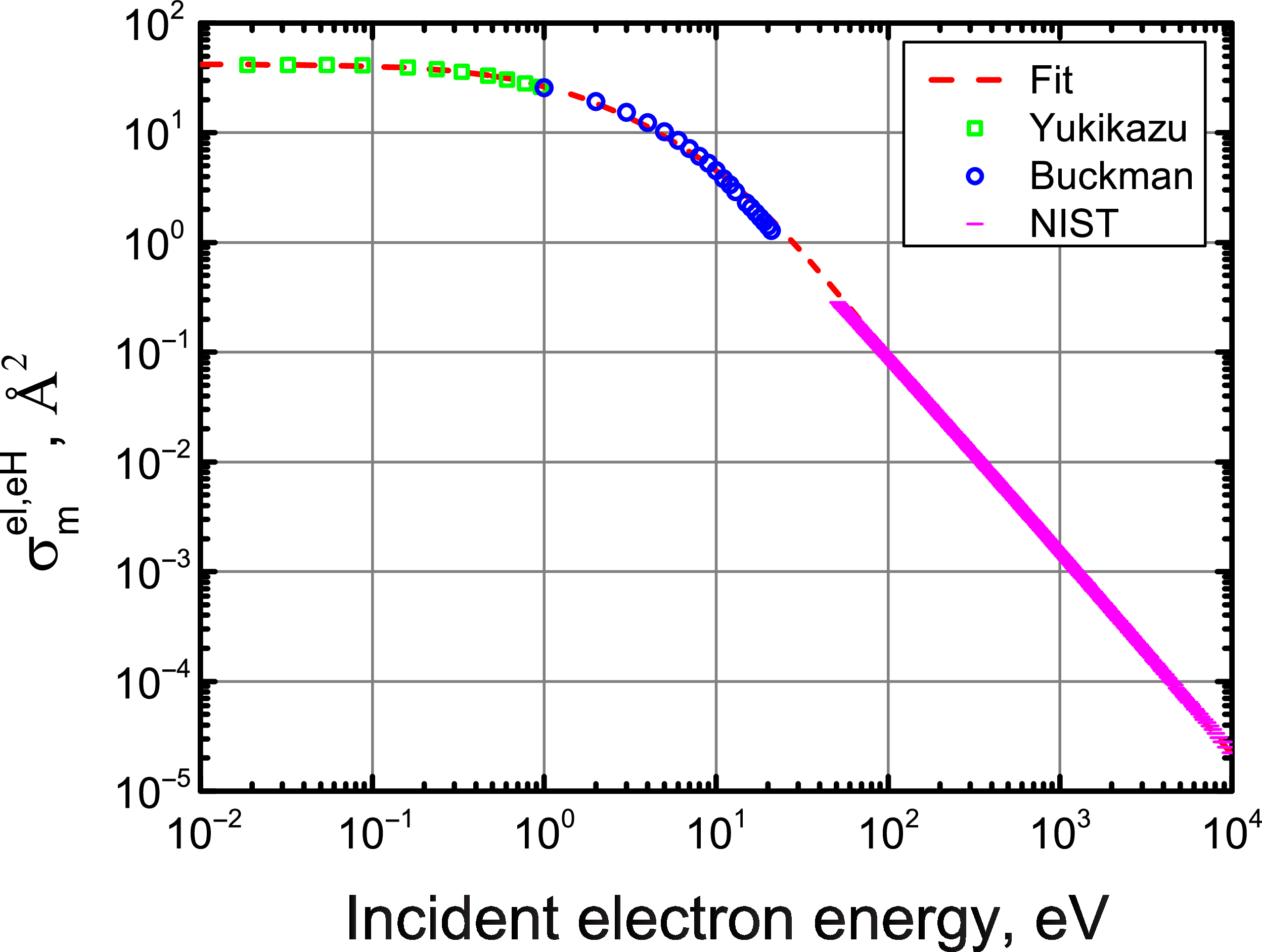

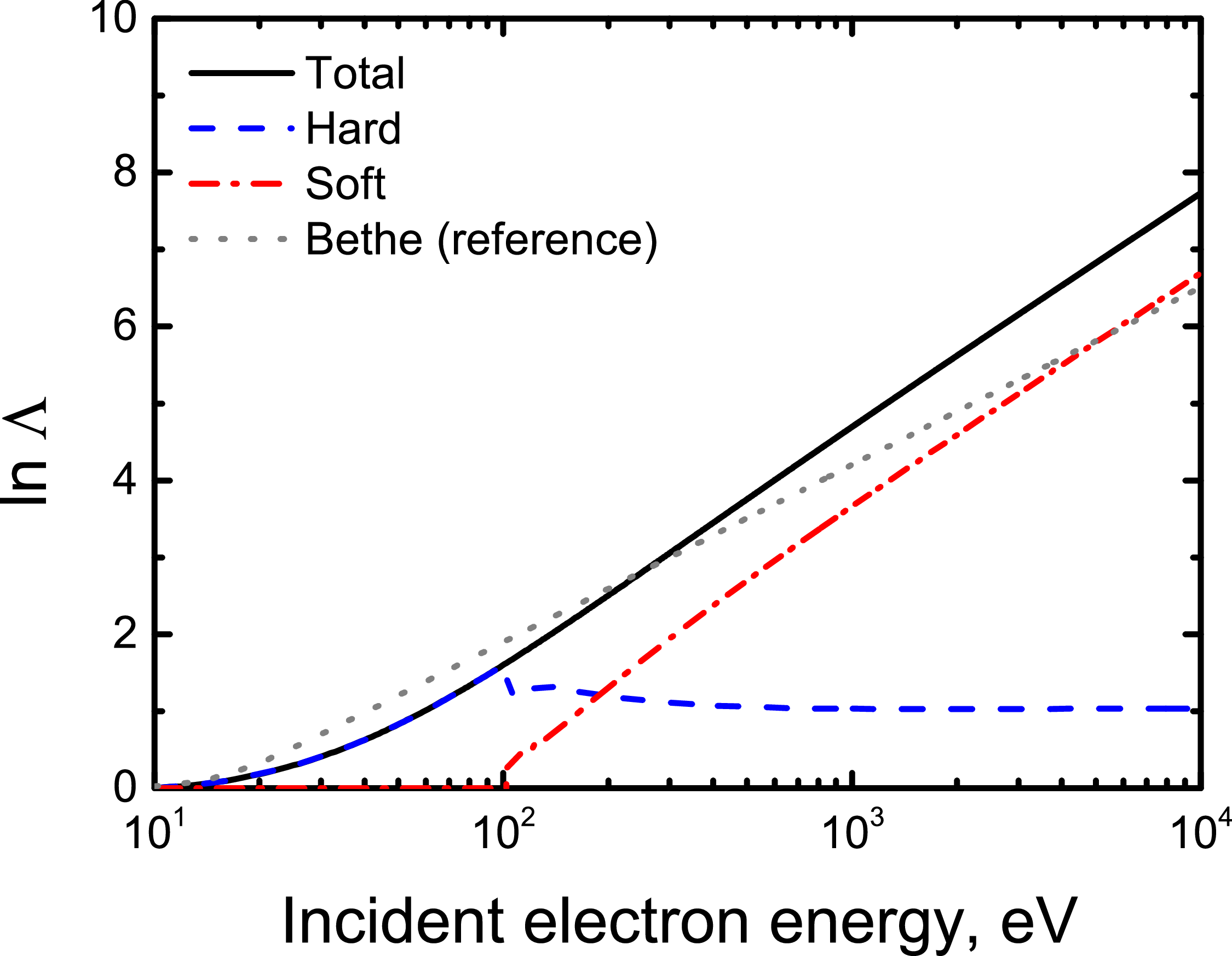


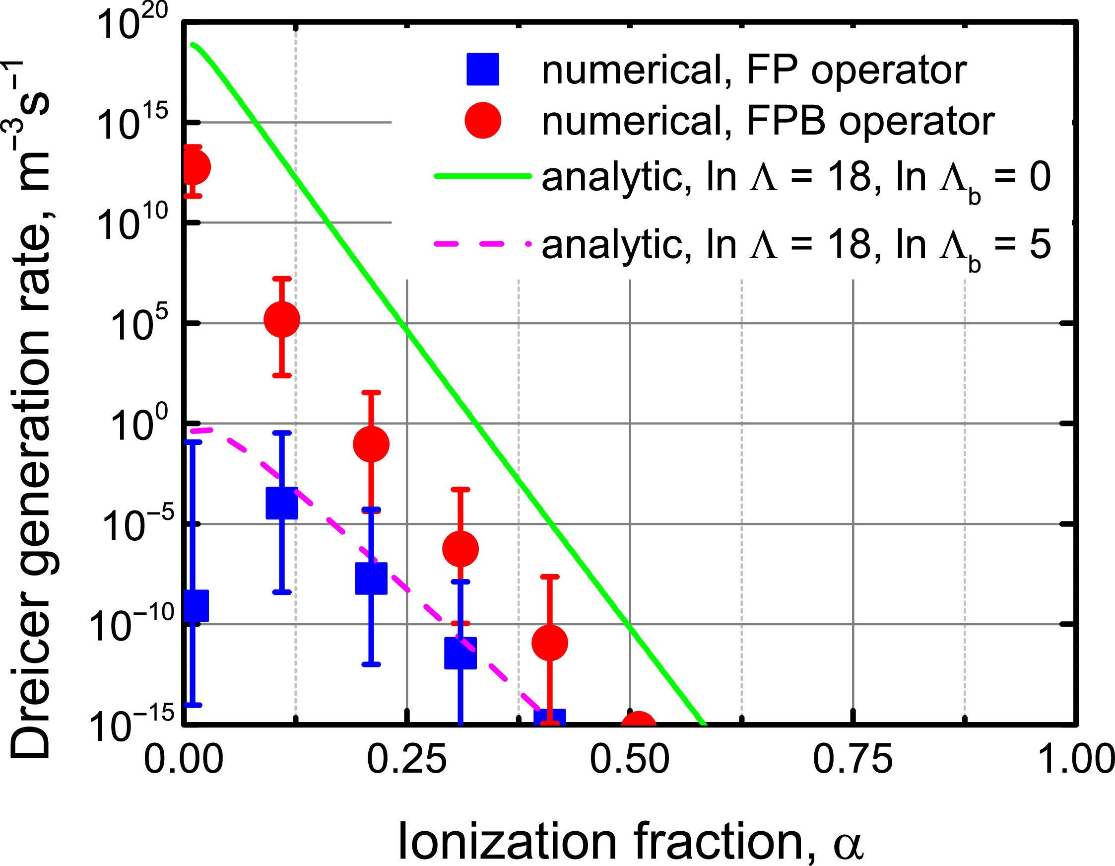


 Open access