


1 Introduction
The two-boost problem goes back to the classical work of W. Hohmann on the attainability of heavenly bodies [Reference Hohmann9]. Although this work was written more than four decades before the first human being stepped on the moon, the Hohmann transfer is still one of the crucial ingredients in space mission design, see e.g. [Reference Vallado and McClain16]. The Hohmann transfer is a transfer between two circular orbits in the Kepler problem with the help of a Kepler ellipse which is tangent to the two circles. It requires two tangential boosts, one to transfer from the first circle to the ellipse and a second one to transfer from the ellipse to the second circle. Given two points in the plane different from the origin, there always exists a conic section through the two points with focus at the origin. This means that for the Kepler problem, two points in the phase space can always be connected with the help of two boosts. The motivating question for this paper is whether this continues to hold for more general systems.
The general setup for the two-boost problem is as follows. Consider the cotangent bundle
$T^*Q$
 of a manifold Q with its canonical exact symplectic form
$\omega =d\unicode{x3bb} $
of a manifold Q with its canonical exact symplectic form
$\omega =d\unicode{x3bb} $
 ,
$\unicode{x3bb} =p\,dq$
,
$\unicode{x3bb} =p\,dq$
 , and a Hamiltonian
$H:T^*Q\to \mathbb {R}$
, and a Hamiltonian
$H:T^*Q\to \mathbb {R}$
 . Given two points
$q_0,q_1\in Q$
. Given two points
$q_0,q_1\in Q$
 and an energy value c, the two-boost problem asks for the existence of a Hamiltonian orbit of energy c connecting the cotangent fibres
$T_{q_0}^*Q$
and an energy value c, the two-boost problem asks for the existence of a Hamiltonian orbit of energy c connecting the cotangent fibres
$T_{q_0}^*Q$
 and
$T_{q_1}^*Q$
and
$T_{q_1}^*Q$
 . Such orbits arise as critical points of the Rabinowitz action functional

associated to the path space

Thus, the two-boost problem has a positive answer whenever the corresponding Lagrangian Rabinowitz Floer homology
$\mathrm { LRFH}_*(\mathcal {A}^{H_0-h}_{q_0,q_1})$
 is well defined and non-trivial.
As observed in [Reference Cieliebak and Frauenfelder4], the well-definedness of (Lagrangian) Rabinowitz Floer homology requires some hypothesis on the Hamiltonian H. A suitable class is formed by magnetic Hamiltonians

for a magnetic potential
$A\in \Omega ^1(Q)$
 , a potential
$V:Q\to \mathbb {R}$
, a potential
$V:Q\to \mathbb {R}$
 and a Riemannian metric on Q. (As is customary in celestial mechanics, our V is minus the physical potential.) Under the assumption that the underlying manifold Q is compact, the Rabinowitz Floer homology of such Hamiltonians (with possibly non-compact magnetic field) has been studied in [Reference Cieliebak, Frauenfelder and Paternain5] for the periodic case and in [Reference Merry11] for the Lagrangian case. An important dynamical quantity associated to such a Hamiltonian is its Mañé critical value. By a theorem of W. Merry [Reference Merry11], for c above the Mañé critical value, the Lagrangian Rabinowitz Floer homology
$\mathrm {LRFH}_*(\mathcal {A}^{H-c}_{q_0,q_1})$
and a Riemannian metric on Q. (As is customary in celestial mechanics, our V is minus the physical potential.) Under the assumption that the underlying manifold Q is compact, the Rabinowitz Floer homology of such Hamiltonians (with possibly non-compact magnetic field) has been studied in [Reference Cieliebak, Frauenfelder and Paternain5] for the periodic case and in [Reference Merry11] for the Lagrangian case. An important dynamical quantity associated to such a Hamiltonian is its Mañé critical value. By a theorem of W. Merry [Reference Merry11], for c above the Mañé critical value, the Lagrangian Rabinowitz Floer homology
$\mathrm {LRFH}_*(\mathcal {A}^{H-c}_{q_0,q_1})$
 is well defined and non-trivial; hence, the two-boost problem is solvable.
Returning to celestial mechanics, let us consider the planar circular restricted 3-body problem. Here, two heavy bodies (the primaries) move under their mutual gravitational attraction on circles around their centre of mass in a plane, and the third body (of negligible mass) moves in the same plane under the gravitational attraction by the primaries. In rotating coordinates, this system is described by the autonomous Hamiltonian

where V is the sum of the (negative) Coulomb potentials of the two primaries (see e.g. [Reference Frauenfelder and van Koert8]). Writing it as

with the effective potential
$V_{\mathrm {eff}}(q_1,q_2)=V(q_1,q_2)+\frac 12(q_1^2+q_2^2)$
 , we see that this is a magnetic Hamiltonian, with magnetic field generating the Coriolis force. In contrast to the previous paragraph, the configuration space
$\mathbb {R}^2\setminus \{q_E,q_M\}$
, we see that this is a magnetic Hamiltonian, with magnetic field generating the Coriolis force. In contrast to the previous paragraph, the configuration space
$\mathbb {R}^2\setminus \{q_E,q_M\}$
 is now non-compact due to possible collisions with the primaries at positions
$q_E,q_M$
is now non-compact due to possible collisions with the primaries at positions
$q_E,q_M$
 and possible escapes to infinity. Our goal is to define and compute Lagrangian Rabinowitz Floer homology in this situation. Since the non-compactness due to collisions can be removed by Moser or Levi–Civita regularization (see [Reference Frauenfelder and van Koert8]), respectively Birkhoff regularization (see, for instance, [Reference Cieliebak, Frauenfelder and Zhao6]), which simultaneously regularizes collisions at both primaries, we will focus our attention on the non-compactness at infinity in
$\mathbb {R}^2$
and possible escapes to infinity. Our goal is to define and compute Lagrangian Rabinowitz Floer homology in this situation. Since the non-compactness due to collisions can be removed by Moser or Levi–Civita regularization (see [Reference Frauenfelder and van Koert8]), respectively Birkhoff regularization (see, for instance, [Reference Cieliebak, Frauenfelder and Zhao6]), which simultaneously regularizes collisions at both primaries, we will focus our attention on the non-compactness at infinity in
$\mathbb {R}^2$
 . For this, we consider the quadratic Hamiltonian

where
$(r,\theta )$
 are polar coordinates on the plane and
$(p_r,p_\theta )$
are polar coordinates on the plane and
$(p_r,p_\theta )$
 their conjugate momenta. We introduce the following set of smooth functions constant outside a compact set:

For
$q_0,q_1\in \mathbb {R}^2$
 , we define the Rabinowitz action functional
$\mathcal {A}^{H_0-h}_{q_0,q_1} : \mathscr {H}_{q_0,q_1}\times \mathbb {R} \to \mathbb {R}$
, we define the Rabinowitz action functional
$\mathcal {A}^{H_0-h}_{q_0,q_1} : \mathscr {H}_{q_0,q_1}\times \mathbb {R} \to \mathbb {R}$
 as above, with
$Q=\mathbb {R}^2$
as above, with
$Q=\mathbb {R}^2$
 and
$H-c$
and
$H-c$
 replaced by
$H_0-h$
replaced by
$H_0-h$
 . Our first result is the following theorem.
Theorem 1.1. Fix
$q_0,q_1\in \mathbb {R}^2$
 and let
$H_0$
and let
$H_0$
 be as in (1.1). For every
$h \in \mathcal {H}$
be as in (1.1). For every
$h \in \mathcal {H}$
 , the Lagrangian Rabinowitz Floer homology of
$\mathcal {A}^{H_0-h}_{q_0,q_1}$
, the Lagrangian Rabinowitz Floer homology of
$\mathcal {A}^{H_0-h}_{q_0,q_1}$
 is well defined. Moreover, for any two
$h_0,h_1\in \mathcal {H}$
is well defined. Moreover, for any two
$h_0,h_1\in \mathcal {H}$
 , the Lagrangian Rabinowitz Floer homology of
$\mathcal {A}^{H_0-h_0}_{q_0,q_1}$
, the Lagrangian Rabinowitz Floer homology of
$\mathcal {A}^{H_0-h_0}_{q_0,q_1}$
 and
$\mathcal {A}^{H_0-h_1}_{q_0,q_1}$
and
$\mathcal {A}^{H_0-h_1}_{q_0,q_1}$
 are isomorphic.
We denote the Lagrangian Rabinowitz Floer homology of
$\mathcal {A}^{H_0-h}_{q_0,q_1}$
 by
$\mathrm {LRFH}_*(\mathcal {A}^{H_0-h}_{q_0,q_1})$
by
$\mathrm {LRFH}_*(\mathcal {A}^{H_0-h}_{q_0,q_1})$
 . Here, we use coefficients in
$\mathbb {Z}_2=\mathbb {Z}/2\mathbb {Z}$
. Here, we use coefficients in
$\mathbb {Z}_2=\mathbb {Z}/2\mathbb {Z}$
 and a half-integer grading by Maslov indices (see §2.2). Moreover, it comes with a canonical action filtration. Our next result computes the positive action part in the case where
$q_0\neq q_1$
and a half-integer grading by Maslov indices (see §2.2). Moreover, it comes with a canonical action filtration. Our next result computes the positive action part in the case where
$q_0\neq q_1$
 .
.
Theorem 1.2. For the Hamiltonian
$H_0$
 in (1.1),
$h \in \mathcal {H}$
in (1.1),
$h \in \mathcal {H}$
 and any
$q_0,q_1\in \mathbb {R}^2$
and any
$q_0,q_1\in \mathbb {R}^2$
 with
$q_0\neq q_1$
with
$q_0\neq q_1$
 , the positive Lagrangian Rabinowitz homology of
$\mathcal {A}^{H_0-h}_{q_0,q_1}$
, the positive Lagrangian Rabinowitz homology of
$\mathcal {A}^{H_0-h}_{q_0,q_1}$
 is well defined and equal to

This shows that the two-boost problem at energy
$0$
 is solvable for
$H_0-h$
is solvable for
$H_0-h$
 with
$h\in \mathcal {H}$
with
$h\in \mathcal {H}$
 . Note that
$h(q,p)=c+V(q)$
. Note that
$h(q,p)=c+V(q)$
 belongs to
$\mathcal {H}$
belongs to
$\mathcal {H}$
 for each constant
$c>0$
for each constant
$c>0$
 and compactly supported potential
$V\geq 0$
and compactly supported potential
$V\geq 0$
 , so the two-boost problem is solvable for
$H_0-V$
, so the two-boost problem is solvable for
$H_0-V$
 with such V at each energy
$c>0$
with such V at each energy
$c>0$
 .
.
The potential in the planar circular restricted 3-body problem (after regularization) satisfies
$V\geq 0$
 , but it is not compactly supported. The following result allows us to deal with certain non-compactly supported potentials.
Proposition 1.3. Let
$H_0$
 be the Hamiltonian in (1.1). Fix
$q_0,q_1\in \mathbb {R}^2$
be the Hamiltonian in (1.1). Fix
$q_0,q_1\in \mathbb {R}^2$
 with
$q_0\neq q_1$
with
$q_0\neq q_1$
 and a positive constant
$c>0$
and a positive constant
$c>0$
 . Let
$V: \mathbb {R}^2 \to \mathbb {R}$
. Let
$V: \mathbb {R}^2 \to \mathbb {R}$
 be a non-negative potential for which there exist
$r_0>0$
be a non-negative potential for which there exist
$r_0>0$
 and
$(\alpha , a) \in \{2\}\times (0 ,{c^2}/{4})\cup (2, +\infty ) \times \mathbb {R}_+$
and
$(\alpha , a) \in \{2\}\times (0 ,{c^2}/{4})\cup (2, +\infty ) \times \mathbb {R}_+$
 such that for
$r>r_0$
such that for
$r>r_0$
 , we have

Then, there exists a function
$V_0\in \mathcal {H}$
 such that
$\operatorname {Crit} \mathcal {A}^{H_0-V-c}_{q_0,q_1} = \operatorname {Crit} \mathcal {A}^{H_0-V_0}_{q_0,q_1}$
such that
$\operatorname {Crit} \mathcal {A}^{H_0-V-c}_{q_0,q_1} = \operatorname {Crit} \mathcal {A}^{H_0-V_0}_{q_0,q_1}$
 .
.
In view of Theorem 1.2, the two-boost problem is therefore solvable for
$H_0-V$
 at energy
$c>0$
at energy
$c>0$
 for any
$(V,c)$
for any
$(V,c)$
 as in Proposition 1.3. In particular, this holds for any
$c>0$
as in Proposition 1.3. In particular, this holds for any
$c>0$
 and
$V\geq 0$
and
$V\geq 0$
 which decays at infinity as
$r^{-\alpha }$
which decays at infinity as
$r^{-\alpha }$
 with
$\alpha>2$
with
$\alpha>2$
 . Note that this does not cover the planar circular restricted 3-body problem, in which the potential decays as
$r^{-1}$
. Note that this does not cover the planar circular restricted 3-body problem, in which the potential decays as
$r^{-1}$
 . We defer the extension to this case to future work.
Remark 1.4. Note that for
$h \in \mathcal {H}$
 , the Liouville vector field
$p\partial _p$
, the Liouville vector field
$p\partial _p$
 is transverse to
${(H_0-h)^{-1}(0)}$
is transverse to
${(H_0-h)^{-1}(0)}$
 , so the zero level set of
$H_0-h$
, so the zero level set of
$H_0-h$
 is of restricted contact type. Thus, the solutions of the two-boost problem resulting from Theorem 1.2 and Proposition 1.3 can also be interpreted as solutions of Arnold’s chord conjecture (existence of a Reeb chord connecting two Legendrians) for certain non-compact contact manifolds.
Remark 1.5. Work by R. Nicholls [Reference Nicholls12] provides some evidence that, if defined, the Mañé critical value for the restricted three-body problem should be zero. It would be interesting to make this rigorous by developing a notion of Mañé critical value for magnetic Hamiltonians over non-compact base manifolds.
2 Lagrangian Rabinowitz Floer homology
Lagrangian Rabinowitz Floer homology was first defined by Merry in [Reference Merry11] for virtually exact Lagrangian submanifolds and compact hypersurfaces of virtual contact type in symplectically aspherical symplectic manifolds. In his setting, the pull-back of the symplectic form to the universal cover of the symplectic manifold had to be exact and the pre-image of the chosen hypersurface in the universal cover had to be of contact type. The symplectic manifold and the Lagrangian submanifold could be non-compact, but the chosen hypersurface of virtual contact type had to be compact.
Our aim is to use Lagrangian Rabinowitz Floer homology to analyse the planar circular restricted three body problem. Therefore, we are interested in the setting of a cotangent bundle
$T^*Q$
 with its standard symplectic form and a pair of fibres
$T_{q_0}^*Q, T_{q_1}^*Q$
with its standard symplectic form and a pair of fibres
$T_{q_0}^*Q, T_{q_1}^*Q$
 as the Lagrangians. In this section, we will explain the definition of the Lagrangian Rabinowitz Floer homology in this setting. It is a far easier setting than the one in [Reference Merry11], as the cotangent bundle is an exact manifold and the fibres are exact Lagrangians. Moreover, the positive level sets of the Hamiltonian corresponding to the planar circular restricted three body problem are all of exact contact type (see Remark 1.4). The only challenge of this setting is that all the energy level sets in the restricted three body problem are non-compact. Rabinowitz Floer homology (for periodic orbits) of non-compact energy level sets of ‘tentacular Hamiltonians’ on
$\mathbb {R}^{2n}$
as the Lagrangians. In this section, we will explain the definition of the Lagrangian Rabinowitz Floer homology in this setting. It is a far easier setting than the one in [Reference Merry11], as the cotangent bundle is an exact manifold and the fibres are exact Lagrangians. Moreover, the positive level sets of the Hamiltonian corresponding to the planar circular restricted three body problem are all of exact contact type (see Remark 1.4). The only challenge of this setting is that all the energy level sets in the restricted three body problem are non-compact. Rabinowitz Floer homology (for periodic orbits) of non-compact energy level sets of ‘tentacular Hamiltonians’ on
$\mathbb {R}^{2n}$
 has been defined in [Reference Pasquotto and Wiśniewska13]. However, the Hamiltonian for the planar circular restricted three body problem does not belong to this class, so new arguments are needed for this setting.
2.1 The Lagrangian Rabinowitz action functional
Throughout this section, Q denotes a smooth oriented n-dimensional manifold and
$T^*Q$
 its cotangent bundle equipped with the exact symplectic form
$\omega =d\unicode{x3bb} $
its cotangent bundle equipped with the exact symplectic form
$\omega =d\unicode{x3bb} $
 for the canonical
$1$
for the canonical
$1$
 -form
$\unicode{x3bb} :=p\,dq$
-form
$\unicode{x3bb} :=p\,dq$
 . Fix
$q_0,q_1 \in Q$
. Fix
$q_0,q_1 \in Q$
 and define the space of paths

Consider a Hamiltonian
$H: T^*Q \to \mathbb {R}$
 with regular level set
$H^{-1}(0)$
with regular level set
$H^{-1}(0)$
 . The Lagrangian Rabinowitz action functional
$\mathcal {A}^H_{q_0,q_1}:\mathscr {H}_{q_0,q_1}\times \mathbb {R}\to \mathbb {R}$
. The Lagrangian Rabinowitz action functional
$\mathcal {A}^H_{q_0,q_1}:\mathscr {H}_{q_0,q_1}\times \mathbb {R}\to \mathbb {R}$
 associated to H is defined as

Remark 2.1. We have a natural bijection
$\mathscr {H}_{q_0,q_1}\ni v \mapsto \overline v\in \mathscr {H}_{q_1,q_0}$
 with
$\overline v(t):=v(1-t)$
with
$\overline v(t):=v(1-t)$
 . Then,

The derivative of
$\mathcal {A}^H_{q_0,q_1}$
 in direction
$(\xi , \sigma ) \in T_v \mathscr {H}_{q_0,q_1}\times T_\eta \mathbb {R}$
in direction
$(\xi , \sigma ) \in T_v \mathscr {H}_{q_0,q_1}\times T_\eta \mathbb {R}$
 equals

Here,
$X_H$
 is the Hamiltonian vector field defined by
$dH=-i_{X_H}\omega $
is the Hamiltonian vector field defined by
$dH=-i_{X_H}\omega $
 . Consequently,
$(v,\eta ) \in \operatorname {Crit} (\mathcal {A}^H_{q_0,q_1})$
. Consequently,
$(v,\eta ) \in \operatorname {Crit} (\mathcal {A}^H_{q_0,q_1})$
 if and only if it satisfies

Thus, we can have three types of critical points:
-
• $\eta>0$
 and
$\widetilde v(t):=v(t/\eta )$
is a Hamiltonian chord (that is, an integral curve of
$X_H$
) on
$H^{-1}(0)$
from
$T^*_{q_0}Q$
to
$T_{q_1}^*Q$
;
and
$\widetilde v(t):=v(t/\eta )$
is a Hamiltonian chord (that is, an integral curve of
$X_H$
) on
$H^{-1}(0)$
from
$T^*_{q_0}Q$
to
$T_{q_1}^*Q$
; -
• $\eta <0$
and
$\widetilde v(t):=v(t/\eta )$
is a Hamiltonian chord on
$H^{-1}(0)$
from
$T^*_{q_1}Q$
to
$T_{q_0}^*Q$
; -
• $\eta =0$
and v is a constant path in
$T^*_{q_0}Q\cap T_{q_1}^*Q\cap H^{-1}(0)$
(which can only occur if
$q_0=q_1$
).


In particular, if
$T^*_{q_0}Q \cap H^{-1}(0)=\emptyset $
 or
$T_{q_1}^*Q \cap H^{-1}(0)=\emptyset $
or
$T_{q_1}^*Q \cap H^{-1}(0)=\emptyset $
 , then
$ \operatorname {Crit} (\mathcal {A}^H_{q_0,q_1})=\emptyset $
, then
$ \operatorname {Crit} (\mathcal {A}^H_{q_0,q_1})=\emptyset $
 . Therefore, from now on, we will assume that

To construct Lagrangian Rabinowitz Floer homology, we want the critical set of the action functional to be bounded in
$L^\infty $
 . It is possible to define Lagrangian Rabinowitz Floer homology without this assumption, but the construction is much more challenging, so we postpone it for future projects. In fact, to construct Lagrangian Rabinowitz Floer homology, we will need the boundedness of the critical set of the action functional to persist under compact perturbations of the Hamiltonian. We formalize this in the following definition.
Definition 2.2. Consider a Hamiltonian
$H: T^*Q \to \mathbb {R}$
 such that
$H^{-1}(0)$
such that
$H^{-1}(0)$
 is non-compact. Fix
$q_0,q_1\in T^*Q$
is non-compact. Fix
$q_0,q_1\in T^*Q$
 satisfying (2.2). Let
$K\subseteq T^*Q$
satisfying (2.2). Let
$K\subseteq T^*Q$
 be a compact set and let

be an open neighbourhood of
$0$
 in
$\{ h\in C^\infty (T^*Q)\ |\ dh\in C_0^\infty (K)\}$
in
$\{ h\in C^\infty (T^*Q)\ |\ dh\in C_0^\infty (K)\}$
 . We say that the associated Rabinowitz action functional
$\mathcal {A}^H_{q_0,q_1}:\mathscr {H}_{q_0,q_1}\times \mathbb {R}\to \mathbb {R}$
. We say that the associated Rabinowitz action functional
$\mathcal {A}^H_{q_0,q_1}:\mathscr {H}_{q_0,q_1}\times \mathbb {R}\to \mathbb {R}$
 has critical set continuously compact in
$(K,\mathcal {H})$
has critical set continuously compact in
$(K,\mathcal {H})$
 if
if

2.2 Grading
In [Reference Cieliebak and Frauenfelder4], Rabinowitz Floer homology (for periodic orbits) is equipped with a shifted integer grading under the hypothesis that the ambient symplectic manifold has vanishing first Chern class. In this subsection, we indicate how this carries over to the Lagrangian setting; see [Reference Merry11] for details.
Consider an exact symplectic manifold
$(V,\omega =d\unicode{x3bb} )$
 of dimension
$2n$
of dimension
$2n$
 and a Hamiltonian
$H:V\to \mathbb {R}$
and a Hamiltonian
$H:V\to \mathbb {R}$
 with regular level set
$\Sigma =H^{-1}(0)$
with regular level set
$\Sigma =H^{-1}(0)$
 such that
$\xi =\ker (\unicode{x3bb} |_\Sigma )$
such that
$\xi =\ker (\unicode{x3bb} |_\Sigma )$
 is a contact structure. Consider in addition two Lagrangian submanifolds
$L_0,L_1\subset V$
is a contact structure. Consider in addition two Lagrangian submanifolds
$L_0,L_1\subset V$
 transverse to
$\Sigma $
transverse to
$\Sigma $
 with
$\unicode{x3bb} |_{L_i}=0$
with
$\unicode{x3bb} |_{L_i}=0$
 . We assume that
$L_0$
. We assume that
$L_0$
 and
$L_1$
and
$L_1$
 are either disjoint or equal. The condition of vanishing first Chern class in [Reference Cieliebak and Frauenfelder4] gets replaced by vanishing of the relative first Chern class
$c_1(V,L_0\cup L_1)$
are either disjoint or equal. The condition of vanishing first Chern class in [Reference Cieliebak and Frauenfelder4] gets replaced by vanishing of the relative first Chern class
$c_1(V,L_0\cup L_1)$
 . The transversal Conley–Zehnder index in [Reference Cieliebak and Frauenfelder4] gets replaced by the transverse Maslov index defined as follows. Let
$(v,\eta )$
. The transversal Conley–Zehnder index in [Reference Cieliebak and Frauenfelder4] gets replaced by the transverse Maslov index defined as follows. Let
$(v,\eta )$
 be a critical point of the Rabinowitz action functional
$\mathcal {A}^H$
be a critical point of the Rabinowitz action functional
$\mathcal {A}^H$
 on the space of paths from
$L_0$
on the space of paths from
$L_0$
 to
$L_1$
to
$L_1$
 . Pick a symplectic trivialization
$v^*\xi \cong [0,1]\times \mathbb {R}^{2n-2}$
. Pick a symplectic trivialization
$v^*\xi \cong [0,1]\times \mathbb {R}^{2n-2}$
 sending
$T_{v(i)}L_i\cap \xi _{v(i)}$
sending
$T_{v(i)}L_i\cap \xi _{v(i)}$
 to
$\mathbb {R}^{n-1}$
to
$\mathbb {R}^{n-1}$
 for
$i=0,1$
for
$i=0,1$
 . In this trivialization, the image of
$T_{v(i)}L_i\cap \xi _{v(i)}$
. In this trivialization, the image of
$T_{v(i)}L_i\cap \xi _{v(i)}$
 under the linearized flow of
$\eta X_H$
under the linearized flow of
$\eta X_H$
 gives a path
$\Lambda :[0,1]\to \mathcal {L}_{n-1}$
gives a path
$\Lambda :[0,1]\to \mathcal {L}_{n-1}$
 in the Grassmannian
$\mathcal {L}_{n-1}$
in the Grassmannian
$\mathcal {L}_{n-1}$
 of Lagrangian subspaces of
$(\mathbb {R}^{2n-2},\omega _{\mathrm { std}})$
of Lagrangian subspaces of
$(\mathbb {R}^{2n-2},\omega _{\mathrm { std}})$
 with
$\Lambda (0)=\mathbb {R}^{n-1}$
with
$\Lambda (0)=\mathbb {R}^{n-1}$
 . Let
$\mu ^{\mathrm {tr}}(v,\eta )\in \frac 12\mathbb {Z}$
. Let
$\mu ^{\mathrm {tr}}(v,\eta )\in \frac 12\mathbb {Z}$
 be the Maslov index of the path
$\Lambda $
be the Maslov index of the path
$\Lambda $
 defined by Robbin and Salamon in [Reference Robbin and Salamon14]. By vanishing of
$c_1(V,L_0\cup L_1)$
defined by Robbin and Salamon in [Reference Robbin and Salamon14]. By vanishing of
$c_1(V,L_0\cup L_1)$
 , this is independent of the choices. In the case where
$\eta =0$
, this is independent of the choices. In the case where
$\eta =0$
 (which occurs only if
$L_0=L_1$
(which occurs only if
$L_0=L_1$
 ), v is a critical point of an auxiliary Morse function f on
$L_0\cap \Sigma $
), v is a critical point of an auxiliary Morse function f on
$L_0\cap \Sigma $
 . Its signature index is
$\mathrm {ind}^\sigma _f(v,0) := -\frac 12\mathrm {sign}\,\mathrm {Hess}_f(v)$
. Its signature index is
$\mathrm {ind}^\sigma _f(v,0) := -\frac 12\mathrm {sign}\,\mathrm {Hess}_f(v)$
 and we set it to zero if
$\eta \neq 0$
and we set it to zero if
$\eta \neq 0$
 . According to [Reference Cieliebak and Frauenfelder4, Appendix A], the Maslov index

defines a half-integer grading on the Rabinowitz Floer complex with respect to which the differential has degree
$-1$
 .
.
This discussion applies to the setting in this section where
$V=T^*Q$
 and
$L_i=T_{q_i}^*Q$
and
$L_i=T_{q_i}^*Q$
 for an oriented n-dimensional manifold Q.
Example 2.3. Consider the free Hamiltonian
$H_{{\bullet }}(q,p):=\tfrac 12|p|^2$
 on
$T^*\mathbb {R}^n$
on
$T^*\mathbb {R}^n$
 and fix an energy
$c>0$
and fix an energy
$c>0$
 . Assume first that
$q_0\neq q_1\in \mathbb {R}^n$
. Assume first that
$q_0\neq q_1\in \mathbb {R}^n$
 . Then,
$\mathcal {A}^{H_{{\bullet }}-c}_{q_0,q_1}$
. Then,
$\mathcal {A}^{H_{{\bullet }}-c}_{q_0,q_1}$
 has exactly two critical points
$(v_\pm ,\eta _\pm )$
has exactly two critical points
$(v_\pm ,\eta _\pm )$
 given by

The linearized flow of
$\eta _\pm X_{H_{\bullet }}$
 along
$v_\pm $
along
$v_\pm $
 equals
 ![]() , so the corresponding path of Lagrangian subspaces
$\Lambda :[0,1]\to \mathcal {L}_{n-1}$
, so the corresponding path of Lagrangian subspaces
$\Lambda :[0,1]\to \mathcal {L}_{n-1}$
 is given by
$\Lambda (t)=\Phi _t(\mathbb {R}^{n-1})=\mathrm {graph}\,A(t)$
is given by
$\Lambda (t)=\Phi _t(\mathbb {R}^{n-1})=\mathrm {graph}\,A(t)$
 with
with ![]() . Thus, the (localization) property in [Reference Robbin and Salamon14] yields
. Thus, the (localization) property in [Reference Robbin and Salamon14] yields

In the case where
$q_0=q_1$
 , let f be a Morse function on the
$(n-1)$
, let f be a Morse function on the
$(n-1)$
 -sphere
$T_{q_0}Q\cap H_{\bullet }^{-1}(c)$
-sphere
$T_{q_0}Q\cap H_{\bullet }^{-1}(c)$
 with exactly two critical points, the maximum
$v_+$
with exactly two critical points, the maximum
$v_+$
 and the minimum
$v_-$
and the minimum
$v_-$
 . Then,
$\mathcal {A}^{H_{{\bullet }}-c}_{q_0,q_0}$
. Then,
$\mathcal {A}^{H_{{\bullet }}-c}_{q_0,q_0}$
 has exactly two critical points
$(v_\pm ,0)$
has exactly two critical points
$(v_\pm ,0)$
 of index

For
$q_0\neq q_1$
 , this immediately implies

Moreover, for
$n\neq 3$
 and any
$q_0,q_1$
and any
$q_0,q_1$
 (equal or not), we obtain

(This also holds for
$n=2$
 , but an additional argument is needed to show that the two critical points of index
$\pm 1/2$
, but an additional argument is needed to show that the two critical points of index
$\pm 1/2$
 do not cancel in homology.)
Remark 2.4. The previous example generalizes to the free Hamiltonian
$H_{{\bullet }}(q,p)=\tfrac 12|p|^2$
 on the cotangent bundle of an n-dimensional Riemannian manifold
$(Q,g)$
on the cotangent bundle of an n-dimensional Riemannian manifold
$(Q,g)$
 . For
$q_0\neq q_1$
. For
$q_0\neq q_1$
 and
$(v,\eta )\in \operatorname {Crit}\mathcal {A}^{H_{{\bullet }}-c}_{q_0,q_1}$
and
$(v,\eta )\in \operatorname {Crit}\mathcal {A}^{H_{{\bullet }}-c}_{q_0,q_1}$
 , the path v projects onto a geodesic
$\bar v$
, the path v projects onto a geodesic
$\bar v$
 from
$q_0$
from
$q_0$
 to
$q_1$
to
$q_1$
 and [Reference Robbin and Salamon15, Proposition 6.38] yields

where
$\mathrm {ind}(\bar v)$
 is the Morse index of the geodesic
$\bar v$
is the Morse index of the geodesic
$\bar v$
 (that is, the number of conjugate points along
$\bar v$
(that is, the number of conjugate points along
$\bar v$
 ).
).
2.3 Floer trajectories
In this subsection, we introduce the fundamental notion for constructing any Floer-type homology—the Floer trajectories. We start by equipping the space
$\mathscr {H}_{q_0,q_1}$
 with a metric. An almost complex structure J on a manifold M is a bundle endomorphism
$J: TM \to TM$
with a metric. An almost complex structure J on a manifold M is a bundle endomorphism
$J: TM \to TM$
 satisfying
$J^2 = -\operatorname {Id}$
satisfying
$J^2 = -\operatorname {Id}$
 . An almost complex structure J on a symplectic manifold
$(M, \omega )$
. An almost complex structure J on a symplectic manifold
$(M, \omega )$
 is called compatible if
$\omega (\ \cdot \ ,J \cdot \ )$
is called compatible if
$\omega (\ \cdot \ ,J \cdot \ )$
 defines a Riemannian metric on M. Denote by
$\mathcal {J}(M,\omega )$
defines a Riemannian metric on M. Denote by
$\mathcal {J}(M,\omega )$
 the space of all compatible almost complex structures on
$(M,\omega )$
the space of all compatible almost complex structures on
$(M,\omega )$
 with the
$C^\infty $
with the
$C^\infty $
 -topology. A linear algebra argument [Reference Cannas da Silva3, Proposition 13.1] shows that
$\mathcal {J}(M,\omega )$
-topology. A linear algebra argument [Reference Cannas da Silva3, Proposition 13.1] shows that
$\mathcal {J}(M,\omega )$
 is contractible.
A smooth
$2$
 -parameter family
$\{J_{t,\eta }\}_{(t,\eta )\in [0,1]\times \mathbb {R}}$
-parameter family
$\{J_{t,\eta }\}_{(t,\eta )\in [0,1]\times \mathbb {R}}$
 of compatible almost complex structures on
$(T^*Q, \omega )$
of compatible almost complex structures on
$(T^*Q, \omega )$
 defines an
$L^2$
defines an
$L^2$
 -metric on
$\mathscr {H}_{q_0,q_1}\times \mathbb {R}$
-metric on
$\mathscr {H}_{q_0,q_1}\times \mathbb {R}$
 by
by

for
$(\xi _i,\sigma _i)\in T_{(v,\eta )}(\mathscr {H}_{q_0,q_1}\times \mathbb {R})$
 . The gradient of the Lagrangian Rabinowitz action functional
$\mathcal {A}^H_{q_0,q_1}$
. The gradient of the Lagrangian Rabinowitz action functional
$\mathcal {A}^H_{q_0,q_1}$
 with respect to this metric equals

Fix an open subset
$\mathcal {V}\subseteq T^*Q$
 and
$\mathbb {J}\in \mathcal {J}(T^*Q,\omega )$
and
$\mathbb {J}\in \mathcal {J}(T^*Q,\omega )$
 . We denote by
$\mathcal {J}(\mathcal {V}, \mathbb {J})$
. We denote by
$\mathcal {J}(\mathcal {V}, \mathbb {J})$
 the set of all smooth maps

satisfying

Fix Hamiltonians
$H_\pm $
 and
$J_\pm \in \mathcal {J}(\mathcal {V},\mathbb {J})$
and
$J_\pm \in \mathcal {J}(\mathcal {V},\mathbb {J})$
 . A homotopy from
$(H_-,J_-)$
. A homotopy from
$(H_-,J_-)$
 to
$(H_+,J_+)$
to
$(H_+,J_+)$
 is a smooth family
$\Gamma = \{(H_s, J_s)\}_{s\in \mathbb {R}}$
is a smooth family
$\Gamma = \{(H_s, J_s)\}_{s\in \mathbb {R}}$
 of Hamiltonians and compatible almost complex structures
$J_s\in \mathcal {J}(\mathcal {V},\mathbb {J})$
of Hamiltonians and compatible almost complex structures
$J_s\in \mathcal {J}(\mathcal {V},\mathbb {J})$
 , which agrees with
$(H_-,J_-)$
, which agrees with
$(H_-,J_-)$
 for
$s\leq s_-$
for
$s\leq s_-$
 and with
$(H_+,J_+)$
and with
$(H_+,J_+)$
 for
$s\geq s_+$
for
$s\geq s_+$
 , with some
$s_\pm \in \mathbb {R}$
, with some
$s_\pm \in \mathbb {R}$
 . A solution
$u: \mathbb {R} \to \mathscr {H}_{q_0,q_1} \times \mathbb {R}$
. A solution
$u: \mathbb {R} \to \mathscr {H}_{q_0,q_1} \times \mathbb {R}$
 to the gradient flow equation
$\partial _s u = \nabla \mathcal {A}^{H_s}_{q_0,q_1}(u)$
to the gradient flow equation
$\partial _s u = \nabla \mathcal {A}^{H_s}_{q_0,q_1}(u)$
 is called a Floer trajectory. In other words, a Floer trajectory
$u=(v,\eta ) \in W^{1,2}(\mathbb {R}\times [0,1], T^*Q)\times W^{1,2}(\mathbb {R})$
is called a Floer trajectory. In other words, a Floer trajectory
$u=(v,\eta ) \in W^{1,2}(\mathbb {R}\times [0,1], T^*Q)\times W^{1,2}(\mathbb {R})$
 is a solution to the equations


For
$(x_-, x_+) \in \operatorname {Crit} \mathcal {A}^{H_-}_{q_0,q_1}\times \operatorname {Crit} \mathcal {A}^{H_+}_{q_0,q_1}$
 , we denote the space of Floer trajectories from
$x_-$
, we denote the space of Floer trajectories from
$x_-$
 to
$x_+$
to
$x_+$
 by
by

In case the homotopy
$\Gamma $
 is constant in s, that is,
$H_s\equiv H$
is constant in s, that is,
$H_s\equiv H$
 and
$J_{s,t,\eta }\equiv J \in \mathcal {J}(\mathcal {V},\mathbb {J})$
and
$J_{s,t,\eta }\equiv J \in \mathcal {J}(\mathcal {V},\mathbb {J})$
 for some Hamiltonian H and a compatible almost complex structure J, we denote
$\mathscr {F}_{H,J}(x_-,x_+):=\mathscr {F}_\Gamma (x_-, x_+)$
for some Hamiltonian H and a compatible almost complex structure J, we denote
$\mathscr {F}_{H,J}(x_-,x_+):=\mathscr {F}_\Gamma (x_-, x_+)$
 .
.
Moreover, for every pair
$(a,b)\in \mathbb {R}^2$
 , we denote

Analogously, we denote
$\mathcal {M}^{H,J}(a,b):=\mathcal {M}^\Gamma (a,b)$
 whenever the homotopy
$\Gamma $
whenever the homotopy
$\Gamma $
 is constant in s and equal to the pair
$(H,J)$
is constant in s and equal to the pair
$(H,J)$
 .
.
If a homotopy
$\Gamma $
 is constant in s, then the action increases along Floer trajectories. However, for a non-constant homotopy
$\Gamma $
is constant in s, then the action increases along Floer trajectories. However, for a non-constant homotopy
$\Gamma $
 , this need not be the case. To deal with this phenomenon, we introduce a condition that ensures that the action cannot decrease indefinitely along a Floer trajectory. We say that a homotopy
$\Gamma := \{(H_s, J_s)\}_{s\in \mathbb {R}}$
, this need not be the case. To deal with this phenomenon, we introduce a condition that ensures that the action cannot decrease indefinitely along a Floer trajectory. We say that a homotopy
$\Gamma := \{(H_s, J_s)\}_{s\in \mathbb {R}}$
 with
$H_{\pm }:=\lim _{s\to \pm \infty }H_s$
with
$H_{\pm }:=\lim _{s\to \pm \infty }H_s$
 satisfies the Novikov finiteness condition if for all
$a,b\in \mathbb {R}$
satisfies the Novikov finiteness condition if for all
$a,b\in \mathbb {R}$
 , we have

2.4 Defining Lagrangian Rabinowitz Floer homology
In this subsection, we will recall the construction of the Lagrangian Rabinowitz Floer homology from [Reference Merry11], using standard Floer techniques introduced in Floer’s seminal paper [Reference Floer7] and the techniques typical for the setting of the Rabinowitz action functional from the first two authors’ paper [Reference Cieliebak and Frauenfelder4]. More precisely, we will prove the following theorem.
Theorem 2.5. Consider a cotangent bundle
$(T^*Q,\omega )$
 with its standard symplectic form and a Hamiltonian
$H:T^*Q\to \mathbb {R}$
with its standard symplectic form and a Hamiltonian
$H:T^*Q\to \mathbb {R}$
 with regular level set
$H^{-1}(0)$
with regular level set
$H^{-1}(0)$
 . Fix a pair
$q_0,q_1\in Q$
. Fix a pair
$q_0,q_1\in Q$
 such that both sets
$H^{-1}(0)\cap T^*_{q_0}Q$
such that both sets
$H^{-1}(0)\cap T^*_{q_0}Q$
 and
$H^{-1}(0)\cap T^*_{q_1}Q$
and
$H^{-1}(0)\cap T^*_{q_1}Q$
 are compact and non-empty. Fix a compatible almost complex structure
$\mathbb {J}\in \mathcal {J}(T^*Q,\omega )$
are compact and non-empty. Fix a compatible almost complex structure
$\mathbb {J}\in \mathcal {J}(T^*Q,\omega )$
 . Assume that there exists a compact subset K, an open subset
$\mathcal {V}$
. Assume that there exists a compact subset K, an open subset
$\mathcal {V}$
 satisfying
$K\subseteq \mathcal {V}\subseteq T^*Q$
satisfying
$K\subseteq \mathcal {V}\subseteq T^*Q$
 and an open neighbourhood
$\mathcal {H}\subseteq \{h\in C^\infty (T^*Q)\ |\ dh\in C_0^\infty (K)\}$
and an open neighbourhood
$\mathcal {H}\subseteq \{h\in C^\infty (T^*Q)\ |\ dh\in C_0^\infty (K)\}$
 of
$0$
of
$0$
 such that:
-
(1) for all $h\in \mathcal {H}$
, the Hamiltonian
$H+h$
satisfies (2.2); -
(2) the Rabinowitz action functional $\mathcal {A}^H_{q_0,q_1}:\mathscr {H}_{q_0,q_1}\times \mathbb {R} \to \mathbb {R}$
has critical set continuously compact in
$(K,\mathcal {H})$
; -
(3) for all $h_0,h_1 \in \mathcal {H}$
and
$J_0, J_1 \in \mathcal {J}(\mathcal {V}, \mathbb {J})$
, every homotopy
$\Gamma =\{(H+h_s, J_s)\}_{s\in \mathbb {R}}$
from
$(H+h_0,J_0)$
to
$(H+h_1,J_1)$
satisfies the Novikov finiteness condition (2.5) and for all
$a, b \in \mathbb {R}$
, the space of Floer trajectories
$\mathcal {M}^\Gamma (a,b)$
is bounded in the
$L^\infty $
-norm.


Then, for every
$h\in \mathcal {H}$
 , the Lagrangian Rabinowitz Floer homology
$\mathrm {LRFH}_*(\mathcal {A}^{H+h}_{q_0,q_1})$
, the Lagrangian Rabinowitz Floer homology
$\mathrm {LRFH}_*(\mathcal {A}^{H+h}_{q_0,q_1})$
 is well defined and isomorphic to
$\mathrm {LRFH}_*(\mathcal {A}^{H}_{q_0,q_1})$
is well defined and isomorphic to
$\mathrm {LRFH}_*(\mathcal {A}^{H}_{q_0,q_1})$
 .
.
Proof. We will define Lagrangian Rabinowitz Floer homology in the case where
$q_0\neq q_1$
 and then briefly explain the case where
$q_0=q_1$
and then briefly explain the case where
$q_0=q_1$
 . Therefore, we first assume
$q_0\neq q_1$
. Therefore, we first assume
$q_0\neq q_1$
 .
.
The first step is to show that for
$q_0\neq q_1$
 and generic
$h\in \mathcal {H}$
and generic
$h\in \mathcal {H}$
 , the Lagrangian Rabinowitz action functional
$\mathcal {A}^{H+h}_{q_0,q_1}$
, the Lagrangian Rabinowitz action functional
$\mathcal {A}^{H+h}_{q_0,q_1}$
 is Morse, that is, its Hessian
$\nabla ^2\mathcal {A}^{H+h}_{q_0,q_1}(x)$
is Morse, that is, its Hessian
$\nabla ^2\mathcal {A}^{H+h}_{q_0,q_1}(x)$
 has trivial kernel for all
$x \in \operatorname {Crit} \mathcal {A}^{H+h}_{q_0,q_1}$
has trivial kernel for all
$x \in \operatorname {Crit} \mathcal {A}^{H+h}_{q_0,q_1}$
 . Observe that for
$q_0\neq q_1$
. Observe that for
$q_0\neq q_1$
 , we we have
$\operatorname {Crit} \mathcal {A}^{H+h}_{q_0,q_1} \cap ( \mathscr {H}_{q_0,q_1}\times \{0\})=\emptyset $
, we we have
$\operatorname {Crit} \mathcal {A}^{H+h}_{q_0,q_1} \cap ( \mathscr {H}_{q_0,q_1}\times \{0\})=\emptyset $
 . By a standard Sard–Smale argument [Reference McDuff and Salamon10, Theorem A.51], there exists a residual subset
$\mathcal {H}^{\,\operatorname {reg}}\subseteq \mathcal {H}\subseteq C_0^\infty (K)$
. By a standard Sard–Smale argument [Reference McDuff and Salamon10, Theorem A.51], there exists a residual subset
$\mathcal {H}^{\,\operatorname {reg}}\subseteq \mathcal {H}\subseteq C_0^\infty (K)$
 such that for all
$h \in \mathcal {H}^{\,\operatorname {reg}}$
such that for all
$h \in \mathcal {H}^{\,\operatorname {reg}}$
 , we have

where
$\phi ^t_{H+h}$
 denotes the Hamiltonian flow of
$X_{H+h}$
denotes the Hamiltonian flow of
$X_{H+h}$
 . The condition is equivalent to the triviality of the kernel of the Hessian
$\nabla ^2 \mathcal {A}^{H+h}_{q_0,q_1}(x)$
. The condition is equivalent to the triviality of the kernel of the Hessian
$\nabla ^2 \mathcal {A}^{H+h}_{q_0,q_1}(x)$
 for all
$x \in \operatorname {Crit} \mathcal {A}^{H+h}_{q_0,q_1}$
for all
$x \in \operatorname {Crit} \mathcal {A}^{H+h}_{q_0,q_1}$
 . A straightforward consequence of the Morse property of the Lagrangian Rabinowitz action functional and continuous compactness of the critical set of
$\mathcal {A}^{H}_{q_0,q_1}$
. A straightforward consequence of the Morse property of the Lagrangian Rabinowitz action functional and continuous compactness of the critical set of
$\mathcal {A}^{H}_{q_0,q_1}$
 is that the critical set of
$\mathcal {A}^{H+h}_{q_0,q_1}$
is that the critical set of
$\mathcal {A}^{H+h}_{q_0,q_1}$
 is finite for each
$h \in \mathcal {H}^{\,\operatorname {reg}}$
is finite for each
$h \in \mathcal {H}^{\,\operatorname {reg}}$
 .
.
Fix
$h\in \mathcal {H}^{\,\operatorname {reg}}$
 . Since
$K \subseteq \mathcal {V}$
. Since
$K \subseteq \mathcal {V}$
 , by continuous compactness of the critical set of
$\mathcal {A}^{H}_{q_0,q_1}$
, by continuous compactness of the critical set of
$\mathcal {A}^{H}_{q_0,q_1}$
 in
$(K,\mathcal {H})$
in
$(K,\mathcal {H})$
 for every
$J\in \mathcal {J}(\mathcal {V}, \mathbb {J})$
for every
$J\in \mathcal {J}(\mathcal {V}, \mathbb {J})$
 , we have

Therefore, we can apply the Sard–Smale argument in [Reference McDuff and Salamon10, Theorem A.51] to conclude that there exists a residual set
$\mathcal {J}^{\,\operatorname {reg}}_h\subseteq \mathcal {J}(T^*Q,\omega ,\mathcal {V})$
 such that for all
$x,y\in \operatorname {Crit}\mathcal {A}^{H+h}_{q_0,q_1}$
such that for all
$x,y\in \operatorname {Crit}\mathcal {A}^{H+h}_{q_0,q_1}$
 and all
$J \in \mathcal {J}^{\,\operatorname {reg}}_h$
and all
$J \in \mathcal {J}^{\,\operatorname {reg}}_h$
 , the space of Floer trajectories
$\mathscr {F}_{H+h,J}(x,y)$
, the space of Floer trajectories
$\mathscr {F}_{H+h,J}(x,y)$
 is a transversely cut out smooth manifold.
Let us now fix
$h\in \mathcal {H}^{\,\operatorname {reg}}$
 and
$J\in \mathcal {J}^{\,\operatorname {reg}}_h$
and
$J\in \mathcal {J}^{\,\operatorname {reg}}_h$
 . For every
$x,y\in \operatorname {Crit}\mathcal {A}^{H+h}_{q_0,q_1}$
. For every
$x,y\in \operatorname {Crit}\mathcal {A}^{H+h}_{q_0,q_1}$
 , there is a natural
$\mathbb {R}$
, there is a natural
$\mathbb {R}$
 -action on
$\mathscr {F}_{H+h,J}(x,y)$
-action on
$\mathscr {F}_{H+h,J}(x,y)$
 given by

Denote the quotient space
$\overline {\mathscr {F}}_{H+h,J}(x,y):=\mathscr {F}_{H+h,J}(x,y)/ \mathbb {R}$
 . By [Reference Merry11, Theorem 2.23], for all
$x,y\in \operatorname {Crit}\mathcal {A}^{H+h}_{q_0,q_1}$
. By [Reference Merry11, Theorem 2.23], for all
$x,y\in \operatorname {Crit}\mathcal {A}^{H+h}_{q_0,q_1}$
 with
$x\neq y$
with
$x\neq y$
 , the quotient
$\overline {\mathscr {F}}_{H+h,J}(x,y)$
, the quotient
$\overline {\mathscr {F}}_{H+h,J}(x,y)$
 is also a smooth manifold and its dimension is given by

By condition (3) in Theorem 2.5, for all
$x,y\in \operatorname {Crit}\mathcal {A}^{H+h}_{q_0,q_1}$
 , the space of Floer trajectories
$\mathscr {F}_{H+h,J}(x,y)$
, the space of Floer trajectories
$\mathscr {F}_{H+h,J}(x,y)$
 is bounded in the
$L^\infty $
is bounded in the
$L^\infty $
 -norm. Now, standard compactness arguments (see [Reference Floer7, Proposition 3b] or [Reference Audin and Damian2, Theorem 9.1.7]) imply that
$\overline {\mathscr {F}}_{H+h,J}(x,y)$
-norm. Now, standard compactness arguments (see [Reference Floer7, Proposition 3b] or [Reference Audin and Damian2, Theorem 9.1.7]) imply that
$\overline {\mathscr {F}}_{H+h,J}(x,y)$
 is compact up to breaking in the sense of Floer. If
$\mu (y)-\mu (x)=1$
is compact up to breaking in the sense of Floer. If
$\mu (y)-\mu (x)=1$
 , this means that
$\overline {\mathscr {F}}_{H+h,J}(x,y)$
, this means that
$\overline {\mathscr {F}}_{H+h,J}(x,y)$
 is a finite set of points [Reference Audin and Damian2, Theorem 9.2.1].
Now, we are ready to define Lagrangian Rabinowitz Floer homology. For
$h\in \mathcal {H}^{\,\operatorname {reg}}$
 and
$k\in \mathbb {Z}$
and
$k\in \mathbb {Z}$
 , let
$CF_k(\mathcal {A}^{H+h}_{q_0,q_1})$
, let
$CF_k(\mathcal {A}^{H+h}_{q_0,q_1})$
 be the
$\mathbb {Z}_2$
be the
$\mathbb {Z}_2$
 -vector space of formal sums of the form
$\sum _{x\in S}x$
-vector space of formal sums of the form
$\sum _{x\in S}x$
 , where
$S\subseteq \operatorname {Crit}\mathcal {A}^{H+h}_{q_0,q_1}$
, where
$S\subseteq \operatorname {Crit}\mathcal {A}^{H+h}_{q_0,q_1}$
 is a (possibly infinite) set satisfying
$\mu (x)=k$
is a (possibly infinite) set satisfying
$\mu (x)=k$
 for all
$x\in S$
for all
$x\in S$
 and the Novikov finiteness condition

Now, we fix an almost complex structure
$J\in \mathcal {J}^{\,\operatorname {reg}}_h$
 and turn
$CF(\mathcal {A}^{H+h}_{q_0,q_1})$
and turn
$CF(\mathcal {A}^{H+h}_{q_0,q_1})$
 into a chain complex. For
$x,y\in \operatorname {Crit}\mathcal {A}^{H+h}_{q_0,q_1}$
into a chain complex. For
$x,y\in \operatorname {Crit}\mathcal {A}^{H+h}_{q_0,q_1}$
 with
$\mu (y)-\mu (x)=1$
with
$\mu (y)-\mu (x)=1$
 , we set

The Floer boundary operator
$\partial _k^J: CF_k(\mathcal {A}^{H+h}_{q_0,q_1})\to CF_{k-1}(\mathcal {A}^{H+h}_{q_0,q_1})$
 is the linear map defined on generators by

Compactness up to breaking implies that
$\partial _k^J\circ \partial _{k+1}^J=0$
 , so we can define the Lagrangian Rabinowitz Floer homology

A standard continuation argument shows that the Lagrangian Rabinowitz Floer homology does not depend on the choice of
$h\in \mathcal {H}^{\,\operatorname {reg}}$
 and
$J\in \mathcal {J}^{\,\operatorname {reg}}_h$
and
$J\in \mathcal {J}^{\,\operatorname {reg}}_h$
 . For this, let
$h_i\in \mathcal {H}^{\,\operatorname {reg}}$
. For this, let
$h_i\in \mathcal {H}^{\,\operatorname {reg}}$
 and
$J_i\in \mathcal {J}^{\,\operatorname {reg}}_{h_i}$
and
$J_i\in \mathcal {J}^{\,\operatorname {reg}}_{h_i}$
 for
$i=0,1$
for
$i=0,1$
 be given. Pick a homotopy
$\Gamma = \{(H+h_s, J_s)\}_{s\in \mathbb {R}}$
be given. Pick a homotopy
$\Gamma = \{(H+h_s, J_s)\}_{s\in \mathbb {R}}$
 connecting
${(H+h_0,J_0)}$
connecting
${(H+h_0,J_0)}$
 to
$(H+h_1,J_1)$
to
$(H+h_1,J_1)$
 as in condition (3) of Theorem 2.5. As before, it follows that for generic
$\Gamma $
as in condition (3) of Theorem 2.5. As before, it follows that for generic
$\Gamma $
 and any pair
$(x,y)\in \operatorname {Crit} \mathcal {A}^{H+h_0}_{q_0,q_1} \times \operatorname {Crit} \mathcal {A}^{H+h_1}_{q_0,q_1}$
and any pair
$(x,y)\in \operatorname {Crit} \mathcal {A}^{H+h_0}_{q_0,q_1} \times \operatorname {Crit} \mathcal {A}^{H+h_1}_{q_0,q_1}$
 , the associated space of Floer trajectories
$\mathscr {F}_\Gamma (x,y)$
, the associated space of Floer trajectories
$\mathscr {F}_\Gamma (x,y)$
 is a smooth manifold of dimension
$\mu (y)-\mu (x)$
is a smooth manifold of dimension
$\mu (y)-\mu (x)$
 which is compact up to breaking. In particular, if
$\mu (x)=\mu (y)$
which is compact up to breaking. In particular, if
$\mu (x)=\mu (y)$
 , then
$\mathscr {F}_\Gamma (x,y)$
, then
$\mathscr {F}_\Gamma (x,y)$
 is a finite set of points and we set
$m(x,y):= \# \mathscr {F}_\Gamma (x,y)\mod 2$
is a finite set of points and we set
$m(x,y):= \# \mathscr {F}_\Gamma (x,y)\mod 2$
 . We define a linear map
$\phi ^\Gamma : (CF_*(\mathcal {A}^{H+h_1}_{q_0,q_1}),\partial ^{J_1})\to (CF(\mathcal {A}^{H+h_0}_{q_0,q_1}),\partial ^{J_0})$
. We define a linear map
$\phi ^\Gamma : (CF_*(\mathcal {A}^{H+h_1}_{q_0,q_1}),\partial ^{J_1})\to (CF(\mathcal {A}^{H+h_0}_{q_0,q_1}),\partial ^{J_0})$
 on generators by

Here, the Novikov finiteness condition (2.5) on
$\Gamma $
 ensures that
$\phi ^\Gamma ( CF(\mathcal {A}^{H+h_1}_{q_0,q_1}))\subseteq CF(\mathcal {A}^{H+h_0}_{q_0,q_1})$
ensures that
$\phi ^\Gamma ( CF(\mathcal {A}^{H+h_1}_{q_0,q_1}))\subseteq CF(\mathcal {A}^{H+h_0}_{q_0,q_1})$
 . Compactness up to breaking implies that
$\phi ^\Gamma $
. Compactness up to breaking implies that
$\phi ^\Gamma $
 is a chain map, and composition with a homotopy in the opposite direction shows that
$\phi ^\Gamma $
is a chain map, and composition with a homotopy in the opposite direction shows that
$\phi ^\Gamma $
 induces an isomorphism on homology (see [Reference Audin and Damian2, Ch. 11] for details on this standard argument).
Since
$\mathrm {LRFH}_k(\mathcal {A}^{H+h}_{q_0,q_1};J)$
 does not depend on
$J\in \mathcal {J}^{\,\operatorname {reg}}_h$
does not depend on
$J\in \mathcal {J}^{\,\operatorname {reg}}_h$
 , we can drop J from the notation and write it as
$\mathrm {LRFH}_k(\mathcal {A}^{H+h}_{q_0,q_1})$
, we can drop J from the notation and write it as
$\mathrm {LRFH}_k(\mathcal {A}^{H+h}_{q_0,q_1})$
 . Since this homology is the same vector space for all
${h\in \mathcal {H}^{\,\operatorname {reg}}}$
. Since this homology is the same vector space for all
${h\in \mathcal {H}^{\,\operatorname {reg}}}$
 , we can unambiguously extend it as this vector space to all
$h\in \mathcal {H}$
, we can unambiguously extend it as this vector space to all
$h\in \mathcal {H}$
 . This proves the theorem in the case where
$q_0\neq q_1$
. This proves the theorem in the case where
$q_0\neq q_1$
 .
.
In the case where
$q_0=q_1$
 , by condition (1) for each
$h\in \mathcal {H}$
, by condition (1) for each
$h\in \mathcal {H}$
 , we have critical points
$(v,0)\in \operatorname {Crit}\mathcal {A}^{H+h}_{q_0,q_0}$
, we have critical points
$(v,0)\in \operatorname {Crit}\mathcal {A}^{H+h}_{q_0,q_0}$
 , where v is a constant path in the non-empty transverse intersection
$S_h:=T^*_{q_0}Q\cap (H+h)^{-1}(0)$
, where v is a constant path in the non-empty transverse intersection
$S_h:=T^*_{q_0}Q\cap (H+h)^{-1}(0)$
 . If
$S_h$
. If
$S_h$
 has positive dimension, then the functional
$\mathcal {A}^{H+h}_{q_0,q_0}$
has positive dimension, then the functional
$\mathcal {A}^{H+h}_{q_0,q_0}$
 will only be Morse–Bott for generic
$h\in \mathcal {H}$
will only be Morse–Bott for generic
$h\in \mathcal {H}$
 . This phenomenon is well known in Rabinowitz Floer theory and can be dealt with by picking a Morse function on
$S_h$
. This phenomenon is well known in Rabinowitz Floer theory and can be dealt with by picking a Morse function on
$S_h$
 and counting gradient flow lines with cascades, see [Reference Cieliebak and Frauenfelder4]. With this understood, the rest of the argument works as in the previous case.
Corollary 2.6. Consider the setting from Theorem 2.5. If
$\mathrm {LRFH}_*(\mathcal {A}^{H}_{q_0,q_1})\neq 0$
 , then for every
$h\in \mathcal {H}$
, then for every
$h\in \mathcal {H}$
 , the set of solutions
$\operatorname {Crit}(\mathcal {A}^{H+h}_{q_0,q_1})\neq \emptyset $
, the set of solutions
$\operatorname {Crit}(\mathcal {A}^{H+h}_{q_0,q_1})\neq \emptyset $
 .
.
Proof. Denote by
$\mathcal {H}^{\,\,\operatorname {reg}}$
 the subset of
$\mathcal {H}$
the subset of
$\mathcal {H}$
 consisting of elements satisfying (2.6). If
$h\in \mathcal {H}^{\,\operatorname {reg}}$
consisting of elements satisfying (2.6). If
$h\in \mathcal {H}^{\,\operatorname {reg}}$
 , then we can define
$\mathrm {LRFH}_*(\mathcal {A}^{H+h}_{q_0,q_1})$
, then we can define
$\mathrm {LRFH}_*(\mathcal {A}^{H+h}_{q_0,q_1})$
 as explained in the proof of Theorem 2.5. In particular, the complex of
$\mathrm {LRFH}_*(\mathcal {A}^{H+h}_{q_0,q_1})$
as explained in the proof of Theorem 2.5. In particular, the complex of
$\mathrm {LRFH}_*(\mathcal {A}^{H+h}_{q_0,q_1})$
 is generated by elements of
$\operatorname {Crit}(\mathcal {A}^{H+h}_{q_0,q_1})$
is generated by elements of
$\operatorname {Crit}(\mathcal {A}^{H+h}_{q_0,q_1})$
 . Moreover, by Theorem 2.5,
$\mathrm {LRFH}_*(\mathcal {A}^{H+h}_{q_0,q_1})$
. Moreover, by Theorem 2.5,
$\mathrm {LRFH}_*(\mathcal {A}^{H+h}_{q_0,q_1})$
 is isomorphic to
$\mathrm {LRFH}_*(\mathcal {A}^{H}_{q_0,q_1})\neq 0$
is isomorphic to
$\mathrm {LRFH}_*(\mathcal {A}^{H}_{q_0,q_1})\neq 0$
 . Hence,

Suppose there exists
$h\in \mathcal {H}$
 such that
$\operatorname {Crit}(\mathcal {A}^{H+h}_{q_0,q_1})= \emptyset $
such that
$\operatorname {Crit}(\mathcal {A}^{H+h}_{q_0,q_1})= \emptyset $
 . Then, it automatically satisfies condition (2.6), so by definition, it belongs to
$\mathcal {H}^{\,\operatorname {reg}}$
. Then, it automatically satisfies condition (2.6), so by definition, it belongs to
$\mathcal {H}^{\,\operatorname {reg}}$
 . However, that brings us a contradiction by the argument presented above.
Corollary 2.7. Consider a cotangent bundle
$(T^*Q,\omega )$
 with its standard symplectic form and a Hamiltonian
$H:T^*Q\to \mathbb {R}$
with its standard symplectic form and a Hamiltonian
$H:T^*Q\to \mathbb {R}$
 such that
$H^{-1}(0)$
such that
$H^{-1}(0)$
 is of exact contact type. Assume that there exists an exhausting sequence of compact sets
$\{K_n\}_{n\in \mathbb {N}}$
is of exact contact type. Assume that there exists an exhausting sequence of compact sets
$\{K_n\}_{n\in \mathbb {N}}$
 ,
$K_n\subseteq K_{n+1}\subseteq T^*Q$
,
$K_n\subseteq K_{n+1}\subseteq T^*Q$
 ,
$\bigcup _{n\in \mathbb {N}}K_n=T^*Q$
,
$\bigcup _{n\in \mathbb {N}}K_n=T^*Q$
 and an open neighbourhood
$\mathcal {H}$
and an open neighbourhood
$\mathcal {H}$
 of
$0$
of
$0$
 in
$\{h\in C^\infty (T^*Q)\ |\ dh\in C_c^\infty (T^*Q)\}$
in
$\{h\in C^\infty (T^*Q)\ |\ dh\in C_c^\infty (T^*Q)\}$
 such that for every
$n\in \mathbb {N}$
such that for every
$n\in \mathbb {N}$
 , the sets
$K_n$
, the sets
$K_n$
 and
$\mathcal {H}_n=\{h\in \mathcal {H}\ |\ dh\in C_0^\infty (K_n)\}$
and
$\mathcal {H}_n=\{h\in \mathcal {H}\ |\ dh\in C_0^\infty (K_n)\}$
 satisfy the assumptions of Theorem 2.5. Then, for any
$h\in \mathcal {H}$
satisfy the assumptions of Theorem 2.5. Then, for any
$h\in \mathcal {H}$
 , the Lagrangian Rabinowitz Floer homology
$\mathrm {LRFH}_*(\mathcal {A}^{H+h}_{q_0,q_1})$
, the Lagrangian Rabinowitz Floer homology
$\mathrm {LRFH}_*(\mathcal {A}^{H+h}_{q_0,q_1})$
 is well defined and isomorphic to
$\mathrm {LRFH}_*(\mathcal {A}^{H}_{q_0,q_1})$
is well defined and isomorphic to
$\mathrm {LRFH}_*(\mathcal {A}^{H}_{q_0,q_1})$
 .
.
Proof. Let
$h\in \mathcal {H}$
 . Then, there exists
$n\in \mathbb {N}$
. Then, there exists
$n\in \mathbb {N}$
 such that
$h\in \mathcal {H}_n$
such that
$h\in \mathcal {H}_n$
 . Since
$\mathcal {H}$
. Since
$\mathcal {H}$
 is an open neighbourhood of
$0$
is an open neighbourhood of
$0$
 in
$\{h\in C^\infty (T^*Q)\ |\ dh\in C_c^\infty (T^*Q)\}$
in
$\{h\in C^\infty (T^*Q)\ |\ dh\in C_c^\infty (T^*Q)\}$
 , the set
$\mathcal {H}_n$
, the set
$\mathcal {H}_n$
 is an open neighbourhood of
$0$
is an open neighbourhood of
$0$
 in
$\{h\in C^\infty (T^*Q)\ |\ dh\in C_0^\infty (K_n)\}$
in
$\{h\in C^\infty (T^*Q)\ |\ dh\in C_0^\infty (K_n)\}$
 . By assumption, the sets
$K_n$
. By assumption, the sets
$K_n$
 and
$\mathcal {H}_n$
and
$\mathcal {H}_n$
 satisfy the assumptions of Theorem 2.5. By Theorem 2.5, for every
$h\in \mathcal {H}_n$
satisfy the assumptions of Theorem 2.5. By Theorem 2.5, for every
$h\in \mathcal {H}_n$
 , the Lagrangian Rabinowitz Floer homology
$\mathrm {LRFH}_*(\mathcal {A}^{H+h}_{q_0,q_1})$
, the Lagrangian Rabinowitz Floer homology
$\mathrm {LRFH}_*(\mathcal {A}^{H+h}_{q_0,q_1})$
 is well defined and isomorphic to
$\mathrm {LRFH}_*(\mathcal {A}^{H}_{q_0,q_1})$
is well defined and isomorphic to
$\mathrm {LRFH}_*(\mathcal {A}^{H}_{q_0,q_1})$
 .
.
2.5 Positive Lagrangian Rabinowitz Floer homology
The action functional
$\mathcal {A}^{H}_{q_0,q_1}$
 provides an
$\mathbb {R}$
provides an
$\mathbb {R}$
 -filtration on
$CF_*(\mathcal {A}^{H}_{q_0,q_1})$
-filtration on
$CF_*(\mathcal {A}^{H}_{q_0,q_1})$
 by
by

Since Floer trajectories are defined by the
$L^2$
 -gradient of the action functional, the boundary operator does not increase the action, i.e.

The positive Rabinowitz Floer homology
$\mathrm {LRFH}_*^+(\mathcal {A}^{H}_{q_0,q_1})$
 is the homology of the quotient complex
with boundary operator
$\partial ^{\scriptscriptstyle +}$
 induced by
$\partial $
induced by
$\partial $
 on the quotient.
To get the required transversality in the preceding discussion, we need to replace H by
$H+h$
 with
$h\in \mathcal {H}^{\,\textit{reg}}$
with
$h\in \mathcal {H}^{\,\textit{reg}}$
 as in the previous subsection. To ensure that the positive Lagrangian Rabinowitz Floer homology is independent of the choice of h, we require an additional condition. The regular level set
$H^{-1}(0)$
as in the previous subsection. To ensure that the positive Lagrangian Rabinowitz Floer homology is independent of the choice of h, we require an additional condition. The regular level set
$H^{-1}(0)$
 is said to be of exact contact type if there exists a Liouville vector field Y on
$T^*Q$
is said to be of exact contact type if there exists a Liouville vector field Y on
$T^*Q$
 (satisfying
$L_Y\omega =\omega $
(satisfying
$L_Y\omega =\omega $
 ) such that
$dH(Y)>0$
) such that
$dH(Y)>0$
 along
$H^{-1}(0)$
along
$H^{-1}(0)$
 . Setting
$(\xi ,\sigma )=(Y,\eta )$
. Setting
$(\xi ,\sigma )=(Y,\eta )$
 in (2.1), we get

At critical points, the second term on the left-hand side vanishes and we conclude

The following lemma shows that the exact contact type property provides a set of compactly supported perturbations for which the set of positive action values is bounded away from zero.
Lemma 2.8. Consider a cotangent bundle
$(T^*Q,\omega )$
 with its standard symplectic form and a Hamiltonian
$H:T^*Q\to \mathbb {R}$
with its standard symplectic form and a Hamiltonian
$H:T^*Q\to \mathbb {R}$
 such that
$H^{-1}(0)$
such that
$H^{-1}(0)$
 is of exact contact type. Fix
${q_0,q_1\in Q}$
is of exact contact type. Fix
${q_0,q_1\in Q}$
 with
$q_0\neq q_1$
with
$q_0\neq q_1$
 . Assume that there exists a compact subset
$K\subseteq T^*Q$
. Assume that there exists a compact subset
$K\subseteq T^*Q$
 and an open neighbourhood
$\mathcal {H}$
and an open neighbourhood
$\mathcal {H}$
 of
$0$
of
$0$
 in
$\{h\in C^\infty (T^*Q)\ |\ dh\in C_0^\infty (K)\}$
in
$\{h\in C^\infty (T^*Q)\ |\ dh\in C_0^\infty (K)\}$
 such that for all
$h\in \mathcal {H}$
such that for all
$h\in \mathcal {H}$
 , the following holds:

Then, there exists an open neighbourhood
$\mathcal {O}(K)$
 of
$0$
of
$0$
 in
$\mathcal {H}$
in
$\mathcal {H}$
 such that

Proof. By assumption, there exists a Liouville vector field Y such that
$dH(Y)>0$
 along
$H^{-1}(0)$
along
$H^{-1}(0)$
 . Since K is compact,

For
$h\in \mathcal {H}$
 small enough in the
$C^1$
small enough in the
$C^1$
 -norm, we then have

Denote by
$\mathcal {O}(K)$
 the set of all
$h\in \mathcal {H}$
the set of all
$h\in \mathcal {H}$
 satisfying (2.13). Then,
$\mathcal {O}(K)$
satisfying (2.13). Then,
$\mathcal {O}(K)$
 is an open neighbourhood of
$0$
is an open neighbourhood of
$0$
 in
$\{h\in C^\infty (T^*Q)\ |\ dh\in C_0^\infty (K)\}$
in
$\{h\in C^\infty (T^*Q)\ |\ dh\in C_0^\infty (K)\}$
 . Consider
$h\in \mathcal {O}(K)$
. Consider
$h\in \mathcal {O}(K)$
 such that
$\operatorname {Crit}^+ \mathcal {A}^{H+h}_{q_0,q_1}\neq \emptyset $
such that
$\operatorname {Crit}^+ \mathcal {A}^{H+h}_{q_0,q_1}\neq \emptyset $
 . If
$(v,\eta )\in \operatorname {Crit}^+ \mathcal {A}^{H+h}_{q_0,q_1}$
. If
$(v,\eta )\in \operatorname {Crit}^+ \mathcal {A}^{H+h}_{q_0,q_1}$
 , then
$\eta>0$
, then
$\eta>0$
 in view of (2.10) applied to
$H+h$
in view of (2.10) applied to
$H+h$
 . By (2.11), we have
$v([0,1])\subset K\cap (H+h)^{-1}(0)$
. By (2.11), we have
$v([0,1])\subset K\cap (H+h)^{-1}(0)$
 , so from (2.9) and (2.13), we obtain

However, from
$v(i)\in T_{q_i}^*Q$
 for
$i=0,1$
for
$i=0,1$
 and
$\partial _sv=\eta X_{H+h}(v)$
and
$\partial _sv=\eta X_{H+h}(v)$
 , we deduce

with the positive constants

The two estimates combine to
$|\mathcal {A}^{H+h}_{q_0,q_1}(v,\eta )| \geq \delta \varepsilon /2C>0$
 .
.
The next result provides conditions under which positive Lagrangian Rabinowitz Floer homology is not only well defined, but also independent of the auxiliary choices and invariant under compact perturbations.
Corollary 2.9. Consider the setting as in Theorem 2.5 with sets
$K\subseteq \mathcal {V}\subseteq T^*Q$
 and
$\mathcal {H}\subseteq \{C^\infty (T^*Q)\ |\ dh\in C_0^\infty (K)\}$
and
$\mathcal {H}\subseteq \{C^\infty (T^*Q)\ |\ dh\in C_0^\infty (K)\}$
 . Assume
$q_0\neq q_1$
. Assume
$q_0\neq q_1$
 . Let
$\mathcal {O}\subseteq \mathcal {H}$
. Let
$\mathcal {O}\subseteq \mathcal {H}$
 be an open neighbourhood of
$0$
be an open neighbourhood of
$0$
 such that for every pair
$h_0,h_1 \in \mathcal {O}$
such that for every pair
$h_0,h_1 \in \mathcal {O}$
 , there exists a homotopy
${\Gamma := \{(H+h_s, J_s)\}_{s\in \mathbb {R}}}$
, there exists a homotopy
${\Gamma := \{(H+h_s, J_s)\}_{s\in \mathbb {R}}}$
 satisfying condition (3) of Theorem 2.5, and such that for every
${x\in \operatorname {Crit}^+\mathcal {A}^{H+h_0}_{q_0,q_1}}$
satisfying condition (3) of Theorem 2.5, and such that for every
${x\in \operatorname {Crit}^+\mathcal {A}^{H+h_0}_{q_0,q_1}}$
 and every
$y\in \operatorname {Crit}\mathcal {A}^{H+h_1}_{q_0,q_1}$
and every
$y\in \operatorname {Crit}\mathcal {A}^{H+h_1}_{q_0,q_1}$
 for which
$\mathscr {F}_\Gamma (x,y)\neq \emptyset $
for which
$\mathscr {F}_\Gamma (x,y)\neq \emptyset $
 , we have
${\mathcal {A}^{H+h_1}_{q_0,q_1}(y)>0}$
, we have
${\mathcal {A}^{H+h_1}_{q_0,q_1}(y)>0}$
 .
.
Then, for every
$h\in \mathcal {O}$
 , its positive Lagrangian Rabinowitz Floer homology is well defined, and for every pair
$h_0,h_1 \in \mathcal {O}$
, its positive Lagrangian Rabinowitz Floer homology is well defined, and for every pair
$h_0,h_1 \in \mathcal {O}$
 ,
$\mathrm {LRFH}_*^+(\mathcal {A}^{H+h_0}_{q_0,q_1})$
,
$\mathrm {LRFH}_*^+(\mathcal {A}^{H+h_0}_{q_0,q_1})$
 is isomorphic to
$\mathrm {LRFH}_*^+(\mathcal {A}^{H+h_1}_{q_0,q_1})$
is isomorphic to
$\mathrm {LRFH}_*^+(\mathcal {A}^{H+h_1}_{q_0,q_1})$
 .
.
Proof. By assumption, the critical set of
$\mathcal {A}^H_{q_0,q_1}$
 is continuously compact in
$(K,\mathcal {O})$
is continuously compact in
$(K,\mathcal {O})$
 . Denote by
$\mathcal {O}^{\,\operatorname {reg}}$
. Denote by
$\mathcal {O}^{\,\operatorname {reg}}$
 the subset of
$\mathcal {O}$
the subset of
$\mathcal {O}$
 consisting of all Hamiltonian functions
$h\in \mathcal {O}$
consisting of all Hamiltonian functions
$h\in \mathcal {O}$
 such that
$\mathcal {A}^{H+h}_{q_0,q_1}$
such that
$\mathcal {A}^{H+h}_{q_0,q_1}$
 is Morse. By the standard Sard–Smale argument,
$\mathcal {O}^{\,\operatorname {reg}}$
is Morse. By the standard Sard–Smale argument,
$\mathcal {O}^{\,\operatorname {reg}}$
 is dense in
$\mathcal {O}$
is dense in
$\mathcal {O}$
 . Fix
$h_0,h_1 \in \mathcal {O}^{\,\operatorname {reg}}$
. Fix
$h_0,h_1 \in \mathcal {O}^{\,\operatorname {reg}}$
 . By assumption, there exist
$J_i \in \mathcal {J}_{h_i}^{\,\operatorname {reg}}\subset \mathcal {J}(\mathcal {V}, \mathbb {J})$
. By assumption, there exist
$J_i \in \mathcal {J}_{h_i}^{\,\operatorname {reg}}\subset \mathcal {J}(\mathcal {V}, \mathbb {J})$
 for
$i=0,1$
for
$i=0,1$
 and a homotopy
$\Gamma = \{(H+h_s, J_s)\}_{s\in \mathbb {R}}$
and a homotopy
$\Gamma = \{(H+h_s, J_s)\}_{s\in \mathbb {R}}$
 with
$h_s\in \mathcal {O}$
with
$h_s\in \mathcal {O}$
 and
$J_s\in \mathcal {J}(\mathcal {V}, \mathbb {J})$
and
$J_s\in \mathcal {J}(\mathcal {V}, \mathbb {J})$
 from
$(H+h_0,J_0)$
from
$(H+h_0,J_0)$
 to
$(H+h_1,J_1)$
to
$(H+h_1,J_1)$
 with the following properties:
-
(a) the homotopy $\Gamma $
satisfies the Novikov finiteness condition (2.5); -
(b) for any pair $a,b\in \mathbb {R}$
, the space of Floer trajectories
$\mathcal {M}^\Gamma (a,b)$
is bounded in the
$L^\infty $
-norm; -
(c) for every $x\in \operatorname {Crit}^+\mathcal {A}^{H+h_0}_{q_0,q_1}$
and every
$y\in \operatorname {Crit}\mathcal {A}^{H+h_1}_{q_0,q_1}$
such that
$\mathscr {F}_\Gamma (x,y)\neq \emptyset $
, we have
$\mathcal {A}^{H+h_1}_{q_0,q_1}(y)>0$
.


From properties (a) and (b), we get a chain map
$\phi ^\Gamma : CF_*(\mathcal {A}^{H+h_1}_{q_0,q_1})\to CF_*(\mathcal {A}^{H+h_0}_{q_0,q_1})$
 . It satisfies
$\phi ^\Gamma (CF_*^{\leq 0}(\mathcal {A}^{H+h_1}_{q_0,q_1})) \subseteq CF_*^{\leq 0}(\mathcal {A}^{H+h_0}_{q_0,q_1})$
. It satisfies
$\phi ^\Gamma (CF_*^{\leq 0}(\mathcal {A}^{H+h_1}_{q_0,q_1})) \subseteq CF_*^{\leq 0}(\mathcal {A}^{H+h_0}_{q_0,q_1})$
 , since otherwise, there would exist
${x\in \operatorname {Crit}^+\mathcal {A}^{H+h_0}_{q_0,q_1}}$
, since otherwise, there would exist
${x\in \operatorname {Crit}^+\mathcal {A}^{H+h_0}_{q_0,q_1}}$
 and
$y\in \operatorname {Crit}\mathcal {A}^{H+h_1}_{q_0,q_1}$
and
$y\in \operatorname {Crit}\mathcal {A}^{H+h_1}_{q_0,q_1}$
 such that
$\mathscr {F}_\Gamma (x,y)\neq \emptyset $
such that
$\mathscr {F}_\Gamma (x,y)\neq \emptyset $
 and
$\mathcal {A}^{H+h_1}_{q_0,q_1}(y)\leq 0$
and
$\mathcal {A}^{H+h_1}_{q_0,q_1}(y)\leq 0$
 , which contradicts property (c). Thus,
$\phi ^\Gamma $
, which contradicts property (c). Thus,
$\phi ^\Gamma $
 descends to a chain map
$\phi ^\Gamma _+ : CF_*^+(\mathcal {A}^{H+h_1}_{q_0,q_1})\to CF_*^+(\mathcal {A}^{H+h_0}_{q_0,q_1})$
descends to a chain map
$\phi ^\Gamma _+ : CF_*^+(\mathcal {A}^{H+h_1}_{q_0,q_1})\to CF_*^+(\mathcal {A}^{H+h_0}_{q_0,q_1})$
 , and the usual argument using a homotopy in the opposite direction (see [Reference Audin and Damian2, Proposition 11.2.9]) shows that the induced map on homology
$\Phi ^\Gamma _+ \colon \mathrm {LRFH}_*^+(\mathcal {A}^{H+h_1}_{q_0,q_1})\to \mathrm {LRFH}_*^+(\mathcal {A}^{H+h_0}_{q_0,q_1})$
, and the usual argument using a homotopy in the opposite direction (see [Reference Audin and Damian2, Proposition 11.2.9]) shows that the induced map on homology
$\Phi ^\Gamma _+ \colon \mathrm {LRFH}_*^+(\mathcal {A}^{H+h_1}_{q_0,q_1})\to \mathrm {LRFH}_*^+(\mathcal {A}^{H+h_0}_{q_0,q_1})$
 is an isomorphism.
Corollary 2.10. Consider the setting as in Corollary 2.9. If
$\mathrm {LRFH}_*^+(\mathcal {A}^{H}_{q_0,q_1})\neq 0$
 , then for every
$h\in \mathcal {O}$
, then for every
$h\in \mathcal {O}$
 , we have
$\operatorname {Crit}^+\mathcal {A}^{H+h}_{q_0,q_1} \neq \emptyset $
, we have
$\operatorname {Crit}^+\mathcal {A}^{H+h}_{q_0,q_1} \neq \emptyset $
 .
.
The proof of this corollary follows the arguments presented in the proof of Corollary 2.6.
3 Bounds on the Floer trajectories
The aim of this section is to show that the Hamiltonian
$H_0$
 defined in (1.1) together with the set of compactly supported perturbations defined in (1.2) satisfy the assumptions of Theorem 2.5, to apply it and prove Theorem 1.1.
We will start by showing that the necessary condition for the existence of Reeb chords on
$(H_0-h)^{-1}(0)$
 between any two cotangent fibres
$T_{q_0}\mathbb {R}^2$
between any two cotangent fibres
$T_{q_0}\mathbb {R}^2$
 and
$T_{q_1}\mathbb {R}^2$
and
$T_{q_1}\mathbb {R}^2$
 , assumption (1) of Theorem 2.5 holds true in our setting. Next, we will prove that the second assumption of Theorem 2.5 holds true in our setting, that is, the critical set of the Lagrangian Rabinowitz action functional is bounded in
$L^\infty $
, assumption (1) of Theorem 2.5 holds true in our setting. Next, we will prove that the second assumption of Theorem 2.5 holds true in our setting, that is, the critical set of the Lagrangian Rabinowitz action functional is bounded in
$L^\infty $
 . It is possible to define the Lagrangian Rabinowitz Floer homology without this assumption as a limit of homologies defined in an action window, but this is more involved and we postpone it to a future paper.
The most challenging part, which will occupy most of this section, is to prove that the Floer trajectories are uniformly bounded in the
$L^\infty $
 -norm. This is essential in first defining the Lagrangian Rabinowitz homology and then constructing the isomorphism from Theorem 1.1.
Lemma 3.1. Let
$H_0$
 be the Hamiltonian defined in (1.1) and let
$\mathcal {H}$
be the Hamiltonian defined in (1.1) and let
$\mathcal {H}$
 be the set of perturbations defined in (1.2). Then, the set
$(H_0-h)^{-1}(0)\cap T_q\mathbb {R}^2$
be the set of perturbations defined in (1.2). Then, the set
$(H_0-h)^{-1}(0)\cap T_q\mathbb {R}^2$
 is compact and non-empty for every
$h\in \mathcal {H}$
is compact and non-empty for every
$h\in \mathcal {H}$
 and every
$q\in \mathbb {R}^2$
and every
$q\in \mathbb {R}^2$
 .
.
Proof. Fix
$q\in \mathbb {R}^2$
 . Since h is constant outside a compact set, we have

However, we have
$h>0$
 by assumption and
$H_0(q,0)=0$
by assumption and
$H_0(q,0)=0$
 ; hence,

Consequently, by the intermediate value theorem, there exists
$p\in T_q\mathbb {R}^2$
 such that
$H_0(q,p)-h(q,p)=0$
such that
$H_0(q,p)-h(q,p)=0$
 .
.
The following lemma proves that Hamiltonian
$H_0$
 together with the set of compactly supported perturbations defined in (1.2) satisfies the second assumption of Theorem 2.5.
Lemma 3.2. Let
$H_0:T^*\mathbb {R}^2 \to \mathbb {R}$
 be the Hamiltonian defined in (1.1). Fix two points
$q_0,q_1\in \mathbb {R}^2$
be the Hamiltonian defined in (1.1). Fix two points
$q_0,q_1\in \mathbb {R}^2$
 . For
$n\in \mathbb {N}$
. For
$n\in \mathbb {N}$
 and
$m>0$
and
$m>0$
 , denote
$r_n := \max \{|q_0|,|q_1|\}+n$
, denote
$r_n := \max \{|q_0|,|q_1|\}+n$
 and define the compact set
$K_{n,m} \subseteq T^*\mathbb {R}^2$
and define the compact set
$K_{n,m} \subseteq T^*\mathbb {R}^2$
 by
by

Then, for every
$h \in \mathcal {H}$
 such that
$dh \in C_0^\infty ( K_{n,m})$
such that
$dh \in C_0^\infty ( K_{n,m})$
 and
$\|h\|_{L^\infty }<m$
and
$\|h\|_{L^\infty }<m$
 and any
$(v,\eta )\in \operatorname {Crit} \mathcal {A}^{H_0-h}_{q_0,q_1}$
and any
$(v,\eta )\in \operatorname {Crit} \mathcal {A}^{H_0-h}_{q_0,q_1}$
 , we have
$v([0,1])\subseteq K_{n,m}$
, we have
$v([0,1])\subseteq K_{n,m}$
 .
.
Proof. We will use the Poisson bracket defined by
$\{f,g\}=\omega (X_f,X_g)=dg(X_f)$
 . Using (1.1), we calculate

Thus, at a point where
$\{H_0, r\}=0$
 and
$\{\{H_0,\{H_0, r\}\}\leq 0$
and
$\{\{H_0,\{H_0, r\}\}\leq 0$
 , we have
$p_r=p_\theta =0$
, we have
$p_r=p_\theta =0$
 . Since
$H_0(r,\theta , 0, 0) = 0$
. Since
$H_0(r,\theta , 0, 0) = 0$
 , this implies that for each constant
$c>0$
, this implies that for each constant
$c>0$
 , we have

Let now
$(v, \eta ) \in \operatorname {Crit} \mathcal {A}^{H_0-h}_{q_0,q_1}$
 . We will first show that

Arguing by contradiction, suppose that
$r\circ v(t_0)=\max r \circ v> r_n$
 for some
$t_0\in [0,1]$
for some
$t_0\in [0,1]$
 . Since
$r\circ v(i)=|q_i|<r_n$
. Since
$r\circ v(i)=|q_i|<r_n$
 for
$i=0,1$
for
$i=0,1$
 , we have
$t_0\in (0,1)$
, we have
$t_0\in (0,1)$
 and the condition that
$r\circ v$
and the condition that
$r\circ v$
 attains its maximum at
$t_0$
attains its maximum at
$t_0$
 gives
gives

and

The definition of
$K_{n,m}$
 and
$dh \in C_0^\infty ( K_{n,m})$
and
$dh \in C_0^\infty ( K_{n,m})$
 implies that h is equal to a constant
$c>0$
implies that h is equal to a constant
$c>0$
 near
$v(t_0)$
near
$v(t_0)$
 and can therefore be ignored in the Poisson brackets, and we obtain a contradiction to (3.1).
For the bounds on
$p_r\circ v$
 and
$p_\theta \circ v$
and
$p_\theta \circ v$
 , recall that
$v(t)\in (H_0-h)^{-1}(0)$
, recall that
$v(t)\in (H_0-h)^{-1}(0)$
 for all
$t\in [0, 1]$
for all
$t\in [0, 1]$
 . Consequently, we have


Before formulating the main theorem of this section, we will first introduce the following notation. First, to avoid unnecessary clutter, we will abbreviate
$\mathcal {A}^{H_0-h}:=\mathcal {A}^{H_0-h}_{q_0,q_1}$
 as in this section, dependence on
$q_0,q_1\in \mathbb {R}^2$
as in this section, dependence on
$q_0,q_1\in \mathbb {R}^2$
 is not very relevant. Next, recall the set
$\mathcal {H}$
is not very relevant. Next, recall the set
$\mathcal {H}$
 from (1.2). For a compact subset of
$K\subseteq T^*\mathbb {R}^2$
from (1.2). For a compact subset of
$K\subseteq T^*\mathbb {R}^2$
 , we define

Moreover, for an open precompact subset
$\mathcal {V}\subseteq T^*\mathbb {R}^2$
 , we denote by
$\mathcal {J}(\mathcal {V},\mathbb {J})$
, we denote by
$\mathcal {J}(\mathcal {V},\mathbb {J})$
 the set of all the
$2$
the set of all the
$2$
 -parameter families of
$\omega _0$
-parameter families of
$\omega _0$
 -compatible almost complex structures on
$(T^*\mathbb {R}^2, \omega _0)$
-compatible almost complex structures on
$(T^*\mathbb {R}^2, \omega _0)$
 which are equal to the standard complex structure
$\mathbb {J}$
which are equal to the standard complex structure
$\mathbb {J}$
 outside of
$\mathcal {V}$
outside of
$\mathcal {V}$
 (see the definition in §2.3).
Theorem 3.3. Let
$H_0$
 be the Hamiltonian defined in (1.1) and let
$h_0,h_1 \in \mathcal {H}$
be the Hamiltonian defined in (1.1) and let
$h_0,h_1 \in \mathcal {H}$
 . Fix two points
$q_0,q_1 \in \mathbb {R}^2$
. Fix two points
$q_0,q_1 \in \mathbb {R}^2$
 . Let K be a compact subset of
$T^*\mathbb {R}^2$
. Let K be a compact subset of
$T^*\mathbb {R}^2$
 such that for
$i=0,1$
such that for
$i=0,1$
 , it satisfies

Let
$\mathcal {V}\subseteq T^*\mathbb {R}^2$
 be an open, but precompact subset such that
$K\subseteq \mathcal {V}$
be an open, but precompact subset such that
$K\subseteq \mathcal {V}$
 . Let
$\Gamma :=\{(h_s, J_s)\}_{s\in \mathbb {R}}$
. Let
$\Gamma :=\{(h_s, J_s)\}_{s\in \mathbb {R}}$
 be a smooth homotopy of the Hamiltonians
$h_s\in \mathcal {H}(K)$
be a smooth homotopy of the Hamiltonians
$h_s\in \mathcal {H}(K)$
 and
$2$
and
$2$
 -parameter families of almost complex structures
$J_s \in C^\infty ([0,1]\times \mathbb {R},\mathcal {J}(\mathcal {V},\mathbb {J}))$
-parameter families of almost complex structures
$J_s \in C^\infty ([0,1]\times \mathbb {R},\mathcal {J}(\mathcal {V},\mathbb {J}))$
 constant in s outside
$[0,1]$
constant in s outside
$[0,1]$
 such that


Then, for every pair
$(a,b)\in \mathbb {R}^2$
 , the corresponding space
$\mathcal {M}^\Gamma (a,b)$
, the corresponding space
$\mathcal {M}^\Gamma (a,b)$
 of Floer trajectories defined in (2.4) is bounded in the
$L^\infty $
of Floer trajectories defined in (2.4) is bounded in the
$L^\infty $
 -norm.
3.1 The bounds on the action
If the family of Hamiltonians
$\{H_s\}_{s\in \mathbb {R}}$
 is constant in s, that is,
$H_s = H$
is constant in s, that is,
$H_s = H$
 for all
$s\in \mathbb {R}$
for all
$s\in \mathbb {R}$
 , then
$\mathcal {M}^\Gamma (a,b)\neq \emptyset $
, then
$\mathcal {M}^\Gamma (a,b)\neq \emptyset $
 implies
$b>a$
implies
$b>a$
 . However, since in the parametric case the action along the Floer trajectories may not be monotonically increasing, we need to ensure that we have a bound on how much the action can decrease along a Floer trajectory. Proving the bounds on the action conditions will be the main aim of this section.
We will start by proving the following lemma.
Lemma 3.4. For every
$h\in \mathcal {H}$
 ,
,

where
$c:=\inf \{h-dh(p\partial _p\}>0$
 .
.
Proof. Using (1.1), we can compute that the Hamiltonian
$H_0$
 satisfies the following equality:

Combining that with equality (2.9) for all
$(q,p,\eta )=(v,\eta )\in \mathscr {H}_{q_0,q_1}$
 , we obtain


where the last inequality comes from the fact that
$c:=\inf \{h-dh(p\partial _p\}>0$
 .
.
Consequently, for all
$(q,p,\eta )=(v,\eta )\in \mathscr {H}_{q_0,q_1}$
 such that
$\|\nabla \mathcal {A}^{H_0-h}(v,\eta )\|_{L^2\times \mathbb {R}} <1$
such that
$\|\nabla \mathcal {A}^{H_0-h}(v,\eta )\|_{L^2\times \mathbb {R}} <1$
 , we obtain

Now, let us analyse the right-hand side as functions of
$\|p\|_{L^2}$
 :
:

These estimates give the desired inequality.
Lemma 3.5. Consider the setting as in Theorem 3.3. Fix
$a, b\in \mathbb {R}$
 . Then,
$\|\eta \|_{L^\infty }$
. Then,
$\|\eta \|_{L^\infty }$
 ,
$\|\mathcal {A}^{H_0-h_s}\circ u(s)\|_{L^\infty }$
,
$\|\mathcal {A}^{H_0-h_s}\circ u(s)\|_{L^\infty }$
 and
$\|\nabla ^{J_s}\mathcal {A}^{H_0-h_s}\circ u(s)\|_{L^2([0,1])\times \mathbb {R}}$
and
$\|\nabla ^{J_s}\mathcal {A}^{H_0-h_s}\circ u(s)\|_{L^2([0,1])\times \mathbb {R}}$
 are uniformly bounded for all
$u \in \mathcal {M}^\Gamma (a,b)$
are uniformly bounded for all
$u \in \mathcal {M}^\Gamma (a,b)$
 .
.
The following proof follows closely the arguments presented in [Reference Pasquotto and Wiśniewska13, Proposition 3.3]. We will not present all of them here, but we encourage a curious reader to see the details in [Reference Pasquotto and Wiśniewska13].
Proof. Using the fact that
$u\in \mathcal {M}^\Gamma (a,b)$
 is a Floer trajectory, one can calculate the derivative of the action functional over s and obtain the following inequalities (see [Reference Pasquotto and Wiśniewska13, Proposition 3.3]):


In particular, the convergence of the integral

implies that for small enough s, we have
$\|\nabla \mathcal {A}^{H_0-h_{s}}(u(s))\|_{L^{2}\times \mathbb {R}}<1$
 . This ensures that for all
$s \in \mathbb {R}$
. This ensures that for all
$s \in \mathbb {R}$
 , the following value
$\tau _{0}(s)$
, the following value
$\tau _{0}(s)$
 is well defined and finite:

For
$\tau \in [\tau _{0}(s),s]$
 , we have
$\|\nabla \mathcal {A}^{H_0-h_{\tau }}(u(\tau ))\|_{L^{2}\times \mathbb {R}}\geq 1$
, we have
$\|\nabla \mathcal {A}^{H_0-h_{\tau }}(u(\tau ))\|_{L^{2}\times \mathbb {R}}\geq 1$
 , which allows us to estimate (see [Reference Pasquotto and Wiśniewska13, Proposition 3.3])


Now, using the constant
$c>0$
 as in (3.3) together with the the estimates from Lemma 3.4 and (3.6), we can calculate

Since this inequality has to hold for all
$s\in \mathbb {R}$
 , it also has to hold for
$\|\eta \|_{L^\infty }$
, it also has to hold for
$\|\eta \|_{L^\infty }$
 . Using (3.2), we obtain the following estimate:

Now, using (3.2), (3.6), (3.7) and (3.10), we obtain the desired uniform bounds:


Having obtained the bounds on the action, we are ready to prove the Novikov finiteness condition.
Lemma 3.6. Consider the setting as in Theorem 3.3. Then,
$\mathcal {M}_\Gamma (a,b)\neq \emptyset $
 implies

Proof. This proof follows arguments presented in [Reference Cieliebak and Frauenfelder4, Corollary 3.8]. We will prove the first inequality since the second is completely analogous.


However, by (3.2), we have
$\|\partial _sh_s\|_{L^\infty }\leq ({c}/{3})$
 . This, together with (3.7), implies

Now, assume that
$ 3\sqrt {({c}/{2})} \leq a < |b|$
 . To finish the proof, it suffices to exclude the case
$a< - b$
. To finish the proof, it suffices to exclude the case
$a< - b$
 .
.


This, together with (3.2) and (3.7), gives us the following contradiction:

3.2 The set of infinitesimally small action derivation
Let
$H_0$
 be the Hamiltonian defined in (1.1) and let
$\mathcal {H}$
be the Hamiltonian defined in (1.1) and let
$\mathcal {H}$
 be the set of Hamiltonians as in (1.2). For a Hamiltonian
$h \in \mathcal {H}$
be the set of Hamiltonians as in (1.2). For a Hamiltonian
$h \in \mathcal {H}$
 and fixed constants
$\mathfrak {a}, \mathfrak {y}, \varepsilon>0$
and fixed constants
$\mathfrak {a}, \mathfrak {y}, \varepsilon>0$
 , we define the following set:

We will call this set the set of infinitesimally small action derivation.
The main aim of this subsection will be to prove the following proposition.
Proposition 3.7. For fixed constants
$\mathfrak {a}, \mathfrak {y}>0$
 and
$\varepsilon>0$
and
$\varepsilon>0$
 small enough, the corresponding set
$\mathcal {B}_h(\mathfrak {a}, \mathfrak {y}, \varepsilon )$
small enough, the corresponding set
$\mathcal {B}_h(\mathfrak {a}, \mathfrak {y}, \varepsilon )$
 is bounded both in the
$L^{\infty }\times \mathbb {R}$
is bounded both in the
$L^{\infty }\times \mathbb {R}$
 -norm and in the
$L^2\times \mathbb {R}$
-norm and in the
$L^2\times \mathbb {R}$
 -norm.
We will prove Proposition 3.7 in a series of smaller lemmas.
Lemma 3.8. Let
$h\in \mathcal {H}$
 and let
$c:=\inf \{h-dh(p\partial _p)\}>0$
and let
$c:=\inf \{h-dh(p\partial _p)\}>0$
 . If we fix
$\mathfrak {a}, \mathfrak {y}, \varepsilon>0$
. If we fix
$\mathfrak {a}, \mathfrak {y}, \varepsilon>0$
 , then for every
$(q,p,\eta ) \in \mathcal {B}_h (\mathfrak {a}, \mathfrak {y}, \varepsilon )$
, then for every
$(q,p,\eta ) \in \mathcal {B}_h (\mathfrak {a}, \mathfrak {y}, \varepsilon )$
 , we have

Proof. Using (3.5) for
$(q,p,\eta ) \in \mathcal {B}_h (\mathfrak {a}, \mathfrak {y}, \varepsilon )$
 , we obtain

Now, we would like to estimate the maximum of the function on the right-hand side of the inequality:

This gives us the bound on
$|\eta | \|p\|_{L^2}$
 , that is, the first inequality.
Let us denote

Then, we can estimate

Lemma 3.9. If we fix
$\mathfrak {a}, \mathfrak {y}, \varepsilon>0$
 , then for every
$(q,p,\eta ) \in \mathcal {B}_h (\mathfrak {a}, \mathfrak {y}, \varepsilon )$
, then for every
$(q,p,\eta ) \in \mathcal {B}_h (\mathfrak {a}, \mathfrak {y}, \varepsilon )$
 , we have

Proof. First, observe that

Therefore, for all
$t\in [0,1]$
 , we have

where the last inequality was obtained using the result from Lemma 3.8. Integrating both sides, we obtain

By solving this quadratic inequality, we obtain the following bound:

By repeating this procedure with the equation
$|q(t)|^2=|q_1|^2-2\int _t^1 q\partial _tq$
 , we obtain the bound on
$\|q\|_{L^2}$
, we obtain the bound on
$\|q\|_{L^2}$
 for which we were looking.
To obtain the bound for
$\|q\|_{L^\infty }$
 , we will use (3.15) again:

Analogously as before, we repeat this procedure with the equation
$|q(t)|^2=|q_1|^2-2\int _t^1 q\partial _tq$
 to obtain the bound on
$\|q\|_{L^\infty }$
to obtain the bound on
$\|q\|_{L^\infty }$
 for which we were looking.
Lemma 3.10. If we fix
$\mathfrak {a}, \mathfrak {y}, \varepsilon>0$
 , then for every
$(q,p,\eta ) \in \mathcal {B}_h (\mathfrak {a}, \mathfrak {y}, \varepsilon )$
, then for every
$(q,p,\eta ) \in \mathcal {B}_h (\mathfrak {a}, \mathfrak {y}, \varepsilon )$
 , we have

where

Proof. By (3.4), we have

where
$\mathfrak {q}:=\min \{|q_0|,|q_1|\}+2 (3\varepsilon + {\mathfrak {a}}/{\sqrt {2c}}+\mathfrak {y}\|\nabla h\|_{L^\infty })$
 as in Lemma 3.9. By solving this quadratic inequality, we obtain the following bound:

To prove the second bound, first observe that there exists
$t_0\in [0,1]$
 such that
$|p(t_0)|\leq 2 \mathfrak {q}+\sqrt {2 ( \|h\|_{L^\infty }+c+\varepsilon )}$
such that
$|p(t_0)|\leq 2 \mathfrak {q}+\sqrt {2 ( \|h\|_{L^\infty }+c+\varepsilon )}$
 . Thus, we can estimate

Remark 3.11. Note that in the proof above, we did not use the assumption that
${dh \in C_c^\infty (T^*\mathbb {R}^2)}$
 . Thus, we can conclude that for any
$\mathfrak {a}$
. Thus, we can conclude that for any
$\mathfrak {a}$
 ,
$\mathfrak {y}$
,
$\mathfrak {y}$
 ,
$\varepsilon>0$
,
$\varepsilon>0$
 and any Hamiltonian
$h\in C^\infty (T^*\mathbb {R}^2)\cap W^{1,\infty }(T^*\mathbb {R}^2)$
and any Hamiltonian
$h\in C^\infty (T^*\mathbb {R}^2)\cap W^{1,\infty }(T^*\mathbb {R}^2)$
 such that
$h>0$
such that
$h>0$
 and
$h-dh(p\partial _p)>0$
and
$h-dh(p\partial _p)>0$
 , the corresponding set
$\mathcal {B}_h(\mathfrak {a},\mathfrak {y},\varepsilon )$
, the corresponding set
$\mathcal {B}_h(\mathfrak {a},\mathfrak {y},\varepsilon )$
 is bounded in the
$L^{\infty }\times \mathbb {R}$
is bounded in the
$L^{\infty }\times \mathbb {R}$
 -norm and the
$L^2\times \mathbb {R}$
-norm and the
$L^2\times \mathbb {R}$
 -norm.
Remark 3.12. Note that for
$h \in \mathcal {H}$
 , the bounds on
$\mathcal {B}_h(\mathfrak {a},\mathfrak {y}, \varepsilon )$
, the bounds on
$\mathcal {B}_h(\mathfrak {a},\mathfrak {y}, \varepsilon )$
 depend smoothly on the constants
$\mathfrak {a}$
depend smoothly on the constants
$\mathfrak {a}$
 ,
$\mathfrak {y}$
,
$\mathfrak {y}$
 ,
$\varepsilon $
,
$\varepsilon $
 ,
$c:=\inf \{h-dh(p\partial _p)\}$
,
$c:=\inf \{h-dh(p\partial _p)\}$
 and
$\|h\|_{W^{1,\infty }}$
and
$\|h\|_{W^{1,\infty }}$
 . Thus, if we take a subset
$\mathcal {H}'\subseteq \mathcal {H}$
. Thus, if we take a subset
$\mathcal {H}'\subseteq \mathcal {H}$
 bounded in the
$W^{1,\infty }$
bounded in the
$W^{1,\infty }$
 -norm such that
$\inf _{h\in \mathcal {H}'}\inf \{h-dh)p\partial _p)\}>0$
-norm such that
$\inf _{h\in \mathcal {H}'}\inf \{h-dh)p\partial _p)\}>0$
 , then the corresponding set

will be also bounded in the
$L^{\infty }\times \mathbb {R}$
 -norm and the
$L^2\times \mathbb {R}$
-norm and the
$L^2\times \mathbb {R}$
 -norm.
3.3 The
$L^2$
bounds

The aim of this subsection will be to prove the following proposition.
Proposition 3.13. Consider a setting as in Theorem 3.3. Then, for every pair
$a,b\in \mathbb {R}$
 , the corresponding space
$\mathcal {M}^\Gamma (a,b)$
, the corresponding space
$\mathcal {M}^\Gamma (a,b)$
 is bounded in the
$L^2\times \mathbb {R}$
is bounded in the
$L^2\times \mathbb {R}$
 -norm.
Proof. By Lemma 3.5, there exist
$\mathfrak {a,e, y}>0$
 such that for every
$u:=(v,\eta )\in \mathcal {M}^\Gamma (a,b)$
such that for every
$u:=(v,\eta )\in \mathcal {M}^\Gamma (a,b)$
 , we have

Moreover, by (3.12), the convergence of the integral

implies that for every
$\varepsilon>0$
 , there exists
$s\in \mathbb {R}$
, there exists
$s\in \mathbb {R}$
 small enough such that
$\|\nabla \mathcal {A}^{H_0-h_s} (u(s))\|_{L^{2}\times \mathbb {R}}<\varepsilon $
small enough such that
$\|\nabla \mathcal {A}^{H_0-h_s} (u(s))\|_{L^{2}\times \mathbb {R}}<\varepsilon $
 . This ensures that for all
$s \in \mathbb {R}$
. This ensures that for all
$s \in \mathbb {R}$
 , the following value
$\tau _\varepsilon (s)$
, the following value
$\tau _\varepsilon (s)$
 is well defined and finite:

Note that for all
$\tau \in [\tau _\varepsilon , s]$
 , we have
$\|\nabla \mathcal {A}^{H_0-h_\tau -c}(u(\tau ))\|_{L^{2}\times \mathbb {R}}\geq \varepsilon $
, we have
$\|\nabla \mathcal {A}^{H_0-h_\tau -c}(u(\tau ))\|_{L^{2}\times \mathbb {R}}\geq \varepsilon $
 ; thus, we can estimate

However, we know that


therefore, by Remark 3.12, we know that the set

is bounded in
$L^\infty \times \mathbb {R}$
 - and
$L^2\times \mathbb {R}$
- and
$L^2\times \mathbb {R}$
 -norm. In fact, we can use the same bounds as in Lemmas 3.9 and 3.10, denoting

Now, using (3.16) together with Lemma 3.9, we obtain

Analogously, using Lemma 3.10, we obtain


3.4 The maximum principle
In this section, we will explain how to use Aleksandrov’s maximum principle to find
$L^\infty $
 -bounds on the Floer trajectories outside
$\mathcal {B}^\Gamma (\mathfrak {a}, \mathfrak {y}, \varepsilon )$
-bounds on the Floer trajectories outside
$\mathcal {B}^\Gamma (\mathfrak {a}, \mathfrak {y}, \varepsilon )$
 , following the argument of Abbondandolo and Schwartz in [Reference Abbondandolo and Schwarz1]. The contents of this section are word-for-word from the last author’s paper with Pasquotto and Wiśniewska [Reference Pasquotto and Wiśniewska13], but we include it here for the completeness of the argument.
Theorem 3.14. (Aleksandrov’s maximum principle)
Let
$\Omega $
 be a domain in
$\mathbb {R}^{2}$
be a domain in
$\mathbb {R}^{2}$
 and let
$\rho :\Omega \to \mathbb {R}$
and let
$\rho :\Omega \to \mathbb {R}$
 be a function in
$C^{2}(\Omega )\cap C^(\overline {\Omega })$
be a function in
$C^{2}(\Omega )\cap C^(\overline {\Omega })$
 satisfying the elliptic differential inequality

where
$g\in L^2(\Omega ,\mathbb {R}^2)$
 and
$f\in L_{\operatorname {loc}}^1(\Omega )$
and
$f\in L_{\operatorname {loc}}^1(\Omega )$
 . Then, there exists
$C>0$
. Then, there exists
$C>0$
 which depends only on
$\operatorname {diam}\Omega $
which depends only on
$\operatorname {diam}\Omega $
 and
$\|g\|_{L^2(\Omega )}$
and
$\|g\|_{L^2(\Omega )}$
 such that

provided g and the negative part of f are in
$L^{2}(\Omega )$
 .
.
To apply Aleksandrov’s maximum principle and find
$L^{\infty }$
 bounds on the Floer trajectories, one first has to construct a function F with compact level sets, whose composition with a Floer trajectory
$u= (v,\eta )\in \mathscr {H}_{q_0,q_1}\times \mathbb {R}$
bounds on the Floer trajectories, one first has to construct a function F with compact level sets, whose composition with a Floer trajectory
$u= (v,\eta )\in \mathscr {H}_{q_0,q_1}\times \mathbb {R}$
 satisfies the elliptic differential inequality

outside of the set of infinitesimal action derivation
$\mathcal {B}^\Gamma (\mathfrak {a},\mathfrak {y},\varepsilon )$
 . More precisely, having proven
$L^\infty $
. More precisely, having proven
$L^\infty $
 -bounds on
$\mathcal {B}^\Gamma (\mathfrak {a},\mathfrak {y},\varepsilon )$
-bounds on
$\mathcal {B}^\Gamma (\mathfrak {a},\mathfrak {y},\varepsilon )$
 , we can choose a compact set
$K_\varepsilon \subseteq T^*\mathbb {R}^2$
, we can choose a compact set
$K_\varepsilon \subseteq T^*\mathbb {R}^2$
 such that for every
$(v,\eta )\in \mathcal {B}^\Gamma (\mathfrak {a},\mathfrak {y},\varepsilon )$
such that for every
$(v,\eta )\in \mathcal {B}^\Gamma (\mathfrak {a},\mathfrak {y},\varepsilon )$
 , we have
$v([0,1])\subseteq K_\varepsilon $
, we have
$v([0,1])\subseteq K_\varepsilon $
 . To obtain uniform
$L^\infty $
. To obtain uniform
$L^\infty $
 -bounds on the set of Floer trajectories
$\mathcal {M}^\Gamma (a,b)$
-bounds on the set of Floer trajectories
$\mathcal {M}^\Gamma (a,b)$
 , it suffices to find a function F with compact level sets whose composition with any Floer trajectory
$u= (v,\eta )\in \mathscr {H}_{q_0,q_1}\times \mathbb {R}$
, it suffices to find a function F with compact level sets whose composition with any Floer trajectory
$u= (v,\eta )\in \mathscr {H}_{q_0,q_1}\times \mathbb {R}$
 satisfies (3.21) on every connected component
$\Omega $
satisfies (3.21) on every connected component
$\Omega $
 of
of

Having such an inequality, one can apply the Aleksandrov maximum principle, which gives us

provided g and the negative part of f are in
$L^{2}(\Omega )$
 .
.
The core of this method is to find a function satisfying all the required properties. The classical approach is to use plurisubharmonic functions.
Definition 3.15. Let
$(M,\omega )$
 be a symplectic manifold and J a compatible almost complex structure. Then, a
$C^{2}$
be a symplectic manifold and J a compatible almost complex structure. Then, a
$C^{2}$
 function
$F:M\to \mathbb {R}$
function
$F:M\to \mathbb {R}$
 is called plurisubharmonic if

where
$d^{\mathbb {C}}F=dF\circ J$
 .
.
Remark 3.16. Let
$(M, \omega )$
 be a symplectic manifold and let J be a compatible almost complex structure on M. Then, a function
$F:M\to \mathbb {R}$
be a symplectic manifold and let J be a compatible almost complex structure on M. Then, a function
$F:M\to \mathbb {R}$
 is plurisubharmonic if and only if its gradient with respect to g is a Liouville vector field.
The reason one uses plurisubharmonic functions is because their composition with a two-dimensional curve
$v:\Omega \to M,\Omega \subseteq \mathbb {R}^2$
 satisfies

In particular, if v is a J-holomorphic curve, then the elliptic inequality is trivially satisfied. Unfortunately, in the case of Floer trajectories, proving the elliptic inequality is a little more complicated. One has to investigate how the plurisubharmonic function interacts with the Hamiltonian vector field, in particular, one needs to understand the functions
$dF(X_H)$
 and
$d^{\mathbb {C}}F(X_H)$
and
$d^{\mathbb {C}}F(X_H)$
 , which appear if we calculate
$d^{\mathbb {C}}(F\circ u)$
, which appear if we calculate
$d^{\mathbb {C}}(F\circ u)$
 .
.
The proof of the following lemma can be found in [Reference Pasquotto and Wiśniewska13, part of the proof of Proposition 7.1].
Lemma 3.17. Let H be a Hamiltonian function on an exact symplectic manifold
$(M, \omega \,{=}\,d\unicode{x3bb} )$
 and let J be a compatible almost complex structure on M. Let
$u: \mathbb {R} \times [0,1]\to M \times \mathbb {R}$
and let J be a compatible almost complex structure on M. Let
$u: \mathbb {R} \times [0,1]\to M \times \mathbb {R}$
 be a Floer trajectory satisfying
$\partial _s u =\nabla \mathcal {A}^H(u)$
be a Floer trajectory satisfying
$\partial _s u =\nabla \mathcal {A}^H(u)$
 (with constant H and J). Then, for a plurisubharmonic function
$F: M \to \mathbb {R}$
(with constant H and J). Then, for a plurisubharmonic function
$F: M \to \mathbb {R}$
 , we have

3.5 The
$L^\infty $
bounds

In this subsection, we will apply the maximum principle explained in the previous subsection to the setting of the Floer trajectories from
$\mathcal {M}^\Gamma (a,b)$
 to establish the
$L^\infty $
to establish the
$L^\infty $
 -bounds.
Proof of Theorem 3.3
Let
$\Gamma :={(h_s,J_s)}_{s\in \mathbb {R}}$
 be a smooth homotopy of Hamiltonians
${h_s\in \mathcal {H}}$
be a smooth homotopy of Hamiltonians
${h_s\in \mathcal {H}}$
 and almost complex structures
$J_s\in C^\infty ([0,1]\times \mathbb {R}, \mathcal {J}(\mathcal {V},\mathbb {J}))$
and almost complex structures
$J_s\in C^\infty ([0,1]\times \mathbb {R}, \mathcal {J}(\mathcal {V},\mathbb {J}))$
 satisfying (3.2). Here,
$\mathcal {V}\subseteq T^*\mathbb {R}^2$
satisfying (3.2). Here,
$\mathcal {V}\subseteq T^*\mathbb {R}^2$
 is the open, but pre-compact subset defined in Theorem 3.3 with the property that for all
$s\in [0,1]$
is the open, but pre-compact subset defined in Theorem 3.3 with the property that for all
$s\in [0,1]$
 ,
$\operatorname {supp} dh_s\subseteq \mathcal {V}$
,
$\operatorname {supp} dh_s\subseteq \mathcal {V}$
 and
$J_s|_{T^*\mathbb {R}^2\setminus \mathcal {J}}\equiv \mathbb {J}$
and
$J_s|_{T^*\mathbb {R}^2\setminus \mathcal {J}}\equiv \mathbb {J}$
 .
.
Let
$c>0$
 be as in (3.3). If we fix
$a,b \in \mathbb {R}$
be as in (3.3). If we fix
$a,b \in \mathbb {R}$
 , then by Lemma 3.5 we know that there exists
$\mathfrak {y,a,e}>0$
, then by Lemma 3.5 we know that there exists
$\mathfrak {y,a,e}>0$
 , which depend only on
$a,b,c$
, which depend only on
$a,b,c$
 and
$\|J\|_\infty $
and
$\|J\|_\infty $
 such that

However, if we fix
$\varepsilon>0$
 , then by Proposition 3.7 and Remark 3.12, we know that the set
$\mathcal {B}^\Gamma (\mathfrak {a},\mathfrak {y},\varepsilon )$
, then by Proposition 3.7 and Remark 3.12, we know that the set
$\mathcal {B}^\Gamma (\mathfrak {a},\mathfrak {y},\varepsilon )$
 , defined in (3.17), is bounded in the
$L^\infty \times \mathbb {R}$
, defined in (3.17), is bounded in the
$L^\infty \times \mathbb {R}$
 norm and the bounds depend only on
$a,b,\varepsilon $
norm and the bounds depend only on
$a,b,\varepsilon $
 and
$\Gamma $
and
$\Gamma $
 . Consequently, there exists a compact subset
$K_\varepsilon \subseteq T^*\mathbb {R}^2$
. Consequently, there exists a compact subset
$K_\varepsilon \subseteq T^*\mathbb {R}^2$
 such that

Without loss of generality, we assume that
$\overline {\mathcal {V}} \subseteq K_\varepsilon $
 .
.
Let us fix a Floer trajectory
$u=(v,\eta )\in \mathcal {M}^\Gamma (a,b)$
 and denote a connected component

By assumption,
$\operatorname {supp} dh_s \subseteq \overline {V} \subseteq K_\varepsilon $
 ; hence,
$dh_s \circ v |_{\Omega }\equiv 0$
; hence,
$dh_s \circ v |_{\Omega }\equiv 0$
 for all
$s\in [0,1]$
for all
$s\in [0,1]$
 . This means that instead of
$H-h_s$
. This means that instead of
$H-h_s$
 , we can use the Hamiltonian
$H_0-\mathbf {c}_s$
, we can use the Hamiltonian
$H_0-\mathbf {c}_s$
 for some positive function
$\mathbf {c}_s>0$
for some positive function
$\mathbf {c}_s>0$
 on
$v(\Omega )$
on
$v(\Omega )$
 , which will simplify our computations. More precisely, for
$(s,t)\in \Omega $
, which will simplify our computations. More precisely, for
$(s,t)\in \Omega $
 , the Floer trajectory
$(v,\eta )$
, the Floer trajectory
$(v,\eta )$
 satisfies

Naturally,
$\mathfrak {c}_s\leq \sup _{s\in [0,1]}\|h_s\|_{L^\infty }$
 .
.
By the convergence of the integral

we know that
$\lim _{s\to \pm \infty }u(s)\in \mathcal {B}^\Gamma (\mathfrak {a},\mathfrak {y},\varepsilon )$
 . Therefore,

Consequently, we have
$\sup _{\partial \Omega }|q(s,t)|\leq \sup _{K_\varepsilon }|q|$
 . Unfortunately, we do not have a uniform bound on
$\sup _{\partial \Omega }|p|$
. Unfortunately, we do not have a uniform bound on
$\sup _{\partial \Omega }|p|$
 . Therefore, we will need to treat the cases of the position and momentum coordinates separately. We introduce the following functions on
$T^*\mathbb {R}^2$
. Therefore, we will need to treat the cases of the position and momentum coordinates separately. We introduce the following functions on
$T^*\mathbb {R}^2$
 :
:

Both of the functions
$F_1$
 and
$F_2$
and
$F_2$
 are plurisubharmonic, since their corresponding gradients
$q\partial _q$
are plurisubharmonic, since their corresponding gradients
$q\partial _q$
 and
$p\partial _p$
and
$p\partial _p$
 are Liouville vector fields (see Remark 3.16).
In Lemma 3.18, we will show that on
$\Omega $
 , the functions
$F_1\circ v$
, the functions
$F_1\circ v$
 and
$F_2\circ v$
and
$F_2\circ v$
 satisfy

In Lemmas 3.22 and 3.24, we will prove that
$f_1$
 and
$f_2$
and
$f_2$
 , respectively, are bounded in the
$W^{1,1}$
, respectively, are bounded in the
$W^{1,1}$
 -norm on
$\Omega $
-norm on
$\Omega $
 and the bounds depend only on
$a,b,c,\varepsilon $
and the bounds depend only on
$a,b,c,\varepsilon $
 and
$\Gamma $
and
$\Gamma $
 , but not on our choice of the Floer trajectory
$u\in \mathcal {M}^\Gamma (a,b)$
, but not on our choice of the Floer trajectory
$u\in \mathcal {M}^\Gamma (a,b)$
 or our choice of the connected component
$\Omega \subseteq (\mathbb {R}\times [0,1] )\setminus v^{-1}(K_\varepsilon )$
or our choice of the connected component
$\Omega \subseteq (\mathbb {R}\times [0,1] )\setminus v^{-1}(K_\varepsilon )$
 . By the continuity of the Sobolev embedding
$W^{1,1}\hookrightarrow L^2$
. By the continuity of the Sobolev embedding
$W^{1,1}\hookrightarrow L^2$
 , we obtain
$L^2$
, we obtain
$L^2$
 -bounds on
$f_1$
-bounds on
$f_1$
 and
$f_2$
and
$f_2$
 .
.
Since we know that
$\sup _{\partial \Omega }|q(s,t)|\leq \sup _{K_\varepsilon }|q|$
 , we can now apply the Alexandrov maximum principle to obtain

and the right-hand side of the inequality does not depend on our choice of the Floer trajectory
$u\in \mathcal {M}^\Gamma (a,b)$
 or our choice of the connected component
$\Omega \subseteq (\mathbb {R}\times [0,1] )\setminus v^{-1}(K_\varepsilon )$
or our choice of the connected component
$\Omega \subseteq (\mathbb {R}\times [0,1] )\setminus v^{-1}(K_\varepsilon )$
 . In other words, we obtain that the set

is bounded in
$\mathbb {R}^2$
 .
.
Now, we would like to establish the
$L^\infty $
 -bounds on the p-variable of the Floer trajectories. To establish uniform bounds on
$F_2 \circ v$
-bounds on the p-variable of the Floer trajectories. To establish uniform bounds on
$F_2 \circ v$
 for the Floer trajectory
$u=(v,\eta )$
for the Floer trajectory
$u=(v,\eta )$
 , we extend the domain of the Floer trajectory
$v:\mathbb {R}\times [0,1]\to T^*\mathbb {R}^2$
, we extend the domain of the Floer trajectory
$v:\mathbb {R}\times [0,1]\to T^*\mathbb {R}^2$
 to a cylinder
${\mathbb {R}\times ([-1,1]/-1\sim 1)}$
to a cylinder
${\mathbb {R}\times ([-1,1]/-1\sim 1)}$
 in the following way:

If we extend the domain
$\Omega $
 to the cylinder
$\mathbb {R}\times ([-1,1]/-1\sim 1)$
to the cylinder
$\mathbb {R}\times ([-1,1]/-1\sim 1)$
 in the following way:

In particular, we have that
$\sup _{\Omega }f\circ v=\sup _\Theta f\circ \bar {v}$
 and
$\|f\circ \bar {v}\|_{L^2(\Theta )}=2\|f\circ v\|_{L^2(\Omega )}$
and
$\|f\circ \bar {v}\|_{L^2(\Theta )}=2\|f\circ v\|_{L^2(\Omega )}$
 for any smooth function
$f\in T^*\mathbb {R}^2$
for any smooth function
$f\in T^*\mathbb {R}^2$
 .
.
After proving in Lemma 3.19 that
$F_2\circ \bar {v}$
 is in
$C^2(\Theta )$
is in
$C^2(\Theta )$
 , we can apply the Aleksandrov maximum principle and obtain

Since the established bounds do not depend on the choice of
$u\in \mathcal {M}^\Gamma (a,b)$
 or the choice of the connected component
$\Omega \subseteq (\mathbb {R}\times [0,1] )\setminus v^{-1}(K_\varepsilon )$
or the choice of the connected component
$\Omega \subseteq (\mathbb {R}\times [0,1] )\setminus v^{-1}(K_\varepsilon )$
 , this concludes the proof that
$\mathcal {M}^\Gamma (a,b)$
, this concludes the proof that
$\mathcal {M}^\Gamma (a,b)$
 is bounded in the
$L^\infty \times \mathbb {R}$
is bounded in the
$L^\infty \times \mathbb {R}$
 -norm.
To complete the proof of Theorem 3.3, we need to prove the following technical lemmas.
Lemma 3.18. Consider the standard symplectic space
$(T^*\mathbb {R}^2, \omega _0)$
 with the Hamiltonian
$H_0$
with the Hamiltonian
$H_0$
 defined as in (1.1), and functions
$F_1$
defined as in (1.1), and functions
$F_1$
 and
$F_2$
and
$F_2$
 defined in (3.27). Let
$u:\mathbb {R} \to \mathscr {H}_{q_0,q_1}\times \mathbb {R}$
defined in (3.27). Let
$u:\mathbb {R} \to \mathscr {H}_{q_0,q_1}\times \mathbb {R}$
 ,
$u=(v,\eta )$
,
$u=(v,\eta )$
 be a Floer trajectory corresponding to the action functional
$\mathcal {A}^{H_0-c}$
be a Floer trajectory corresponding to the action functional
$\mathcal {A}^{H_0-c}$
 , that is, satisfying the relation (3.26). Then,

Proof. Using (1.1), we can calculate that


Plugging these qualities into (3.22) for a Floer trajectory
$u=(v,\eta )$
 satisfying the relation (3.26), we can calculate

Lemma 3.19. Consider the standard symplectic space
$(T^*\mathbb {R}^2, \omega _0)$
 with the Hamiltonian
$H_0$
with the Hamiltonian
$H_0$
 defined as in (1.1). Let
$u:\mathbb {R} \to \mathscr {H}_{q_0,q_1}\times \mathbb {R}$
defined as in (1.1). Let
$u:\mathbb {R} \to \mathscr {H}_{q_0,q_1}\times \mathbb {R}$
 ,
$u=(v,\eta )$
,
$u=(v,\eta )$
 be a Floer trajectory associated to
$\mathcal {A}^{H_0-\mathbf {c}_s}$
be a Floer trajectory associated to
$\mathcal {A}^{H_0-\mathbf {c}_s}$
 , that is, satisfying the relation (3.26) and let
$\bar {v}:\mathbb {R}\times ([-1,1]/-1\sim 1) \to T^*\mathbb {R}^2$
, that is, satisfying the relation (3.26) and let
$\bar {v}:\mathbb {R}\times ([-1,1]/-1\sim 1) \to T^*\mathbb {R}^2$
 be the extension of v defined in (3.28). Then, the composition
$F_2\circ \bar {v}$
be the extension of v defined in (3.28). Then, the composition
$F_2\circ \bar {v}$
 with the function
$F_2:T^*\mathbb {R}^2\to \mathbb {R}$
with the function
$F_2:T^*\mathbb {R}^2\to \mathbb {R}$
 ,
$F(q,p)=\tfrac 12|p|^2$
,
$F(q,p)=\tfrac 12|p|^2$
 is
$C^2$
is
$C^2$
 .
.
Proof. First, observe that
$\bar {v}$
 is continuous. Moreover,
$\bar {v}$
is continuous. Moreover,
$\bar {v}$
 is smooth on
$\mathbb {R}\times ((-1,0)\cup (0,1))$
is smooth on
$\mathbb {R}\times ((-1,0)\cup (0,1))$
 . Therefore,
$F_2\circ \bar {v}$
. Therefore,
$F_2\circ \bar {v}$
 is also everywhere continuous and smooth on
$\mathbb {R}\times ((-1,0)\cup (0,1))$
is also everywhere continuous and smooth on
$\mathbb {R}\times ((-1,0)\cup (0,1))$
 . What is left to check is that
$F_2\circ \bar {v}$
. What is left to check is that
$F_2\circ \bar {v}$
 is
$C^2$
is
$C^2$
 on
$\mathbb {R}\times \{-1,0,1\}$
on
$\mathbb {R}\times \{-1,0,1\}$
 . Note that

Hence, the function
$F_2\circ \bar {v}$
 is
$C^1$
is
$C^1$
 if and only if

By assumption,
$v: \mathbb {R} \to \mathscr {H}_{q_0,q_1}$
 , so
$v(s,0)\equiv q_0$
, so
$v(s,0)\equiv q_0$
 and
$v(s,1)\equiv q_1$
and
$v(s,1)\equiv q_1$
 for all
$s\in \mathbb {R}$
for all
$s\in \mathbb {R}$
 . Consequently,

Now, using the Floer equation (3.26) for the Hamiltonian
$H_0$
 and the relation (3.30), we can calculate for
$t\geq 0$
and the relation (3.30), we can calculate for
$t\geq 0$
 ,
,

Plugging (3.34) into the equation above, we obtain (3.33), which proves that
$F_2\circ \bar {v}$
 is
$C^1$
is
$C^1$
 everywhere.
To prove that
$F_2\circ \bar {v}$
 is
$C^2$
is
$C^2$
 , we first calculate:

Obviously,
$|p|^2$
 does not depend on the sign of
$\partial _tv$
does not depend on the sign of
$\partial _tv$
 . However, the function
$\partial _{tt}\bar {v}= \partial _{tt}v$
. However, the function
$\partial _{tt}\bar {v}= \partial _{tt}v$
 is continuous, since the two negative signs cancel each other. Therefore, the sum of these two functions is also continuous on the whole cylinder
$\mathbb {R}\times ([-1,1]/-1\sim 1)$
is continuous, since the two negative signs cancel each other. Therefore, the sum of these two functions is also continuous on the whole cylinder
$\mathbb {R}\times ([-1,1]/-1\sim 1)$
 .
.
Now,
$({d^2}/{dsdt})F_2\circ \bar {v}$
 is well defined and continuous on the whole
$\mathbb {R}\times ((-1,0)\cup (0,1))$
is well defined and continuous on the whole
$\mathbb {R}\times ((-1,0)\cup (0,1))$
 . However, by (3.33), we obtain that
$({d^2}/{dsdt})F_2\circ v (s,0)= ({d^2}/{dsdt})F_2\circ v (s,1)=0$
. However, by (3.33), we obtain that
$({d^2}/{dsdt})F_2\circ v (s,0)= ({d^2}/{dsdt})F_2\circ v (s,1)=0$
 ; thus,
$({d^2}/{dsdt})F_2\circ \bar {v}$
; thus,
$({d^2}/{dsdt})F_2\circ \bar {v}$
 is a continuous function on the whole cylinder
$\mathbb {R}\times ([-1,1]/-1\sim 1)$
is a continuous function on the whole cylinder
$\mathbb {R}\times ([-1,1]/-1\sim 1)$
 .
.
Finally, we observe that
$({d^2}/{ds^2})(F_2\circ v (s,t))=({d^2}/{ds^2})(F_2\circ v (s,-t))$
 as it does not depend on the sign of the t-variable.
Lemma 3.20. Let
$\Omega \subseteq (\mathbb {R} \times [0,1])\setminus v^{-1}(K_\varepsilon )$
 be a connected component as defined in (3.25). Then, the following values are well defined and finite:

Moreover,
$s_0$
 and
$s_1$
and
$s_1$
 satisfy

Proof. By Lemma 3.5, we obtain uniform bounds on the action, energy and the
$\eta $
 -parameter for all
$u\in \mathcal {M}^\Gamma (a,b)$
-parameter for all
$u\in \mathcal {M}^\Gamma (a,b)$
 . By the convergence of the integral

we know that
$\lim _{s\to \pm \infty }u(s)\in \mathcal {B}^\Gamma (\mathfrak {a},\mathfrak {y},\varepsilon )$
 . For the compact subset
$K_\varepsilon \subseteq T^*\mathbb {R}^2$
. For the compact subset
$K_\varepsilon \subseteq T^*\mathbb {R}^2$
 defined in (3.24), we have
$v([0,1])\subseteq K_\varepsilon $
defined in (3.24), we have
$v([0,1])\subseteq K_\varepsilon $
 for all
$(v,\eta )\in \mathcal {M}^\Gamma (a,b)$
for all
$(v,\eta )\in \mathcal {M}^\Gamma (a,b)$
 . Since
$\Omega \subseteq (\mathbb {R} \times [0,1])\setminus v^{-1}(K_\varepsilon )$
. Since
$\Omega \subseteq (\mathbb {R} \times [0,1])\setminus v^{-1}(K_\varepsilon )$
 , the values
$s_0$
, the values
$s_0$
 and
$s_1$
and
$s_1$
 as in (3.35) are well defined and finite. Moreover, for all
$s\in (s_0,s_1)$
as in (3.35) are well defined and finite. Moreover, for all
$s\in (s_0,s_1)$
 ,
$u(s)\notin \mathcal {B}^\Gamma (\mathfrak {a},\mathfrak {y}, \varepsilon )$
,
$u(s)\notin \mathcal {B}^\Gamma (\mathfrak {a},\mathfrak {y}, \varepsilon )$
 ; therefore, by (3.16), we can estimate

where
$\mathfrak {e}=\|J\|_\infty (b-a+{c}/{3}\mathfrak {y})$
 as in Lemma 3.5.
Lemma 3.21. Consider the setting as in Theorem 3.3. Fix
$a,b\in \mathbb {R}$
 and let
$u\in \mathcal {M}^\Gamma (a,b)$
and let
$u\in \mathcal {M}^\Gamma (a,b)$
 be a Floer trajectory. Let
$\Omega \subseteq (\mathbb {R} \times [0,1])\setminus v^{-1}(K_\varepsilon )$
be a Floer trajectory. Let
$\Omega \subseteq (\mathbb {R} \times [0,1])\setminus v^{-1}(K_\varepsilon )$
 be a connected component as defined in (3.25). Then, the function

is bounded in the
$L^1(\Omega )$
 norm and the bounds do not depend on u or
$\Omega $
norm and the bounds do not depend on u or
$\Omega $
 .
.
Proof. Let
$s_0$
 and
$s_1$
and
$s_1$
 be as in (3.35). Denote
$\overline {\Omega }:= [s_0,s_1]\times [0,1]$
be as in (3.35). Denote
$\overline {\Omega }:= [s_0,s_1]\times [0,1]$
 . Naturally,
$\Omega \subseteq \overline {\Omega }$
. Naturally,
$\Omega \subseteq \overline {\Omega }$
 . Before we estimate
$\|f_1\|_{L^1(\Omega )}$
. Before we estimate
$\|f_1\|_{L^1(\Omega )}$
 , we first use the Cauchy–Schwartz inequality together with (3.12), (3.18), (3.19) and (3.36) to do the following estimates:


Using the bounds obtained above and the inequality (3.10), we can calculate

Lemma 3.22. Consider the setting as in Lemma 3.21. Then, the function
$f_1$
 is bounded in the
$W^{1,1}$
is bounded in the
$W^{1,1}$
 -norm and the bounds do not depend on u or
$\Omega $
-norm and the bounds do not depend on u or
$\Omega $
 .
.
Proof. To prove that
$f_1\in W^{1,1}(\Omega )$
 , we first need to calculate its derivatives:

where the last equality comes from the fact that
$dF_2(X_{H_0})(q,p)=0$
 . Using (3.18), (3.20) and (3.36), we can estimate


Similarly, we have


Using the estimates above and (3.10), we can combine them to obtain a uniform
$L^1$
 -bound on
$\partial _tf_1$
-bound on
$\partial _tf_1$
 :
:

This gives us a bound on
$\|\partial _tf_1\|_{L^1(\Omega )}$
 , which does not depend on the choice of the Floer trajectory u or the connected component
$\Omega $
, which does not depend on the choice of the Floer trajectory u or the connected component
$\Omega $
 .
.
To estimate
$\|\partial _sf_1\|_{L^1(\Omega )}$
 , we first use (3.18) and (3.37) to estimate

Second, we analyse
$\partial _{ss}\eta $
 :
:

Using (3.2), (3.19) and (3.20), we can estimate

Now, we will use the Floer equations, the Cauchy–Schwartz inequality together with (3.12), (3.16), (3.18), (3.19) and (3.31) to calculate the following:

Using the estimates above together with (3.10), (3.43), (3.44) and (3.47), we can estimate

This gives us a bound on
$\|\partial _sf_1\|_{L^1(\Omega )}$
 , which does not depend on the choice of the Floer trajectory u or the connected component
$\Omega $
, which does not depend on the choice of the Floer trajectory u or the connected component
$\Omega $
 .
.
Lemma 3.23. Consider the setting as in Theorem 3.3. Fix
$a,b\in \mathbb {R}$
 and let
$u\in \mathcal {M}^\Gamma (a,b)$
and let
$u\in \mathcal {M}^\Gamma (a,b)$
 be a Floer trajectory. Let
$\Omega \subseteq (\mathbb {R} \times [0,1])\setminus v^{-1}(K_\varepsilon )$
be a Floer trajectory. Let
$\Omega \subseteq (\mathbb {R} \times [0,1])\setminus v^{-1}(K_\varepsilon )$
 be a connected component as defined in (3.25). Then, the function

is bounded in the
$L^1(\Omega )$
 norm and the bounds do not depend on u or
$\Omega $
norm and the bounds do not depend on u or
$\Omega $
 .
.
Proof. To estimate
$\|f_2\|_{L^1(\Omega )}$
 , we use the bounds obtained in (3.10), (3.37), (3.38), (3.39) and (3.41) to calculate

Lemma 3.24. Consider the setting as in Lemma 3.23. Then, the function
$f_2$
 is bounded in the
$W^{1,1}$
is bounded in the
$W^{1,1}$
 -norm and the bounds do not depend on u or
$\Omega $
-norm and the bounds do not depend on u or
$\Omega $
 .
.
Proof. To prove that
$f_2\in W^{1,1}(\Omega )$
 , we first need to calculate its derivatives:

where the last equality comes from (3.30).
Let
$s_0$
 and
$s_1$
and
$s_1$
 be as in (3.35). Denote
$\overline {\Omega }:= [s_0,s_1]\times [0,1]$
be as in (3.35). Denote
$\overline {\Omega }:= [s_0,s_1]\times [0,1]$
 . Naturally,
$\Omega \subseteq \overline {\Omega }$
. Naturally,
$\Omega \subseteq \overline {\Omega }$
 . Before we estimate
$\|\partial _t f_2\|_{L^1(\Omega )}$
. Before we estimate
$\|\partial _t f_2\|_{L^1(\Omega )}$
 , we will first recall (3.31) and (3.32), which give us the following relation:

Further on, we use (3.12), (3.19), (3.40) and (3.44) to calculate the following bounds:

This, together with (3.50), gives us

Similarly, we have

Using the bounds obtained above together with (3.10), (3.42) and (3.45), we can estimate

Before we estimate
$\|\partial _sf_2\|_{L^2}$
 , we first use (3.19), (3.48) and (3.49) to calculate the following bounds:

Finally, using the estimates above together with (3.10), (3.41), (3.44), (3.47) and (3.51), we can calculate

This concludes the proof that
$f_2$
 is bounded in the
$W^{1,1}$
is bounded in the
$W^{1,1}$
 -norm and the bounds do not depend on the choice of the Floer trajectory
$u\in \mathcal {M}^\Gamma (a,b)$
-norm and the bounds do not depend on the choice of the Floer trajectory
$u\in \mathcal {M}^\Gamma (a,b)$
 or the connected component
$\Omega \subseteq \mathbb {R}\times [0,1]\setminus v^{-1}(K_\varepsilon )$
or the connected component
$\Omega \subseteq \mathbb {R}\times [0,1]\setminus v^{-1}(K_\varepsilon )$
 , but only on the constants
$a,b, \varepsilon $
, but only on the constants
$a,b, \varepsilon $
 and the smooth homotopy
$\Gamma $
and the smooth homotopy
$\Gamma $
 .
.
3.6 The Lagrangian Rabinowitz Floer homology of the Hamiltonian
$H_0$

Having proven the
$L^\infty $
 -bounds on the Floer trajectories, we are finally ready to prove the main theorem of this paper.
Proof of Theorem 1.1
Let
$H_0:T^*\mathbb {R}^2\to \mathbb {R}$
 be the Hamiltonian defined in (1.1) and let
$\mathcal {H}$
be the Hamiltonian defined in (1.1) and let
$\mathcal {H}$
 be the set of perturbations as defined in (1.2). Fix a pair
$q_0,q_1\in \mathbb {R}^2$
be the set of perturbations as defined in (1.2). Fix a pair
$q_0,q_1\in \mathbb {R}^2$
 . Let
$\{K_{n,m}\}_{n,m\in \mathbb {N}}$
. Let
$\{K_{n,m}\}_{n,m\in \mathbb {N}}$
 be the sequence of compact sets as in Lemma 3.2 such that

Fix a Hamiltonian
$h_0\in \mathcal {H}$
 and denote
$c(h_0):=\inf (h-dh(p\partial _p))$
and denote
$c(h_0):=\inf (h-dh(p\partial _p))$
 . Naturally,
${c(h_0)>0}$
. Naturally,
${c(h_0)>0}$
 . Let
$K_{n,m}$
. Let
$K_{n,m}$
 be any of the compact sets in the sequence such that
$\operatorname {supp} dh_0\subseteq K_{n,m}$
be any of the compact sets in the sequence such that
$\operatorname {supp} dh_0\subseteq K_{n,m}$
 and
$\|h_0\|_{L^\infty }<m$
and
$\|h_0\|_{L^\infty }<m$
 . Denote

This way,
$\mathcal {H}_{h_0}(K_{n,m})$
 is an open neighbourhood of
$0$
is an open neighbourhood of
$0$
 in
$\{h\in C^\infty (T^*\mathbb {R}^2)\ |\ dh\in C_0^\infty (K_{n,m})\}$
in
$\{h\in C^\infty (T^*\mathbb {R}^2)\ |\ dh\in C_0^\infty (K_{n,m})\}$
 . By Lemma 3.2, the critical set of the action functional
$\mathcal {A}^{H-h_0}_{q_0,q_1}$
. By Lemma 3.2, the critical set of the action functional
$\mathcal {A}^{H-h_0}_{q_0,q_1}$
 is continuously compact in
$(K_{n,m}, \mathcal {H}_{h_0}(K_{n,m}))$
is continuously compact in
$(K_{n,m}, \mathcal {H}_{h_0}(K_{n,m}))$
 . However, by construction, if
$h\in \mathcal {H}_{h_0}(K_{n,m})$
. However, by construction, if
$h\in \mathcal {H}_{h_0}(K_{n,m})$
 , then
$h_0+h\in \mathcal {H}$
, then
$h_0+h\in \mathcal {H}$
 ; hence, by Lemma 3.1, every Hamiltonian
$H_0-h_0-h$
; hence, by Lemma 3.1, every Hamiltonian
$H_0-h_0-h$
 satisfies the condition (2.7). This proves that the compact set
$K_{n,m}$
satisfies the condition (2.7). This proves that the compact set
$K_{n,m}$
 and the set of perturbations
$\mathcal {H}_{h_0}(K_{n,m})$
and the set of perturbations
$\mathcal {H}_{h_0}(K_{n,m})$
 satisfy assumptions (1) and (2) of Theorem 2.5 for the Hamiltonian
$H_0-h_0$
satisfy assumptions (1) and (2) of Theorem 2.5 for the Hamiltonian
$H_0-h_0$
 .
.
Now, if we take any open, pre-compact set
$\mathcal {V}\subseteq T^*\mathbb {R}^2$
 such that
$K_{n,m}\subseteq \mathcal {V}$
such that
$K_{n,m}\subseteq \mathcal {V}$
 , any two almost complex structures
$J_0,J_1\in \mathcal {J}(\mathcal {V},\mathbb {J})$
, any two almost complex structures
$J_0,J_1\in \mathcal {J}(\mathcal {V},\mathbb {J})$
 and any
$h\in \mathcal {H}_{h_0}(K_{n,m})$
and any
$h\in \mathcal {H}_{h_0}(K_{n,m})$
 , then every smooth homotopy
$\Gamma :=\{(h_0+h,J_s)\}_{s\in \mathbb {R}}$
, then every smooth homotopy
$\Gamma :=\{(h_0+h,J_s)\}_{s\in \mathbb {R}}$
 , with
$J_s\in C^\infty ([0,1]\times \mathbb {R},\mathcal {J}(\mathcal {V},\mathbb {J}))$
, with
$J_s\in C^\infty ([0,1]\times \mathbb {R},\mathcal {J}(\mathcal {V},\mathbb {J}))$
 such that

will automatically satisfy condition (3.2). Consequently, by Theorem 3.3 for every pair
$(a,b)\in \mathbb {R}^2$
 , the corresponding space
$\mathcal {M}^\Gamma (a,b)$
, the corresponding space
$\mathcal {M}^\Gamma (a,b)$
 of Floer trajectories is bounded in
$L^\infty $
of Floer trajectories is bounded in
$L^\infty $
 -norm. Therefore, we can apply Theorem 2.5 and conclude that there exists a residual set
$\mathcal {H}^{\,\operatorname {reg}}_{h_0}(K_{n,m})\subseteq \mathcal {H}_{h_0}(K_{n,m})$
-norm. Therefore, we can apply Theorem 2.5 and conclude that there exists a residual set
$\mathcal {H}^{\,\operatorname {reg}}_{h_0}(K_{n,m})\subseteq \mathcal {H}_{h_0}(K_{n,m})$
 such that for every
$h\in \mathcal {H}^{\,\operatorname {reg}}_{h_0}(K_{n,m})$
such that for every
$h\in \mathcal {H}^{\,\operatorname {reg}}_{h_0}(K_{n,m})$
 , the Lagrangian Rabinowitz Floer homology
$\mathrm { LRFH}_*(\mathcal {A}^{H_0-h_0-h}_{q_0,q_1})$
, the Lagrangian Rabinowitz Floer homology
$\mathrm { LRFH}_*(\mathcal {A}^{H_0-h_0-h}_{q_0,q_1})$
 is well defined and independent of the choice of the almost complex structure.
Now, if we fix
$h_1,h_2\in \mathcal {H}^{\,\operatorname {reg}}_{h_0}(K_{n,m})$
 , then we can construct a homotopy
$\Gamma $
, then we can construct a homotopy
$\Gamma $
 satisfying (3.2). Indeed, let
$J_0\in \mathcal {J}^{\,\operatorname {reg}}_{h_0}$
satisfying (3.2). Indeed, let
$J_0\in \mathcal {J}^{\,\operatorname {reg}}_{h_0}$
 and
$J_1\in \mathcal {J}^{\,\operatorname {reg}}_{h_2}$
and
$J_1\in \mathcal {J}^{\,\operatorname {reg}}_{h_2}$
 will be two almost complex structures close enough, so that there exists a smooth homotopy
$\{J_s\}_{s\in \mathbb {R}}$
will be two almost complex structures close enough, so that there exists a smooth homotopy
$\{J_s\}_{s\in \mathbb {R}}$
 with
$J_s\in C^\infty ([0,1]\times \mathbb {R},\mathcal {J}(\mathcal {V},\mathbb {J}))$
with
$J_s\in C^\infty ([0,1]\times \mathbb {R},\mathcal {J}(\mathcal {V},\mathbb {J}))$
 satisfying (3.53) and
$\sup _{s\in \mathbb {R}}\|J_s\|_{L^\infty }<({1}/{\sqrt {6c(h_0)}})$
satisfying (3.53) and
$\sup _{s\in \mathbb {R}}\|J_s\|_{L^\infty }<({1}/{\sqrt {6c(h_0)}})$
 . Moreover, let
$\chi \in C^\infty (\mathbb {R})$
. Moreover, let
$\chi \in C^\infty (\mathbb {R})$
 be a smooth function satisfying
$\|\chi '\|_{L^\infty } \leq 2$
be a smooth function satisfying
$\|\chi '\|_{L^\infty } \leq 2$
 and
and

Define
$h_s:=h_0+h_1(1-\chi (s))+\chi (s)h_2$
 . Then, the smooth homotopy
$\Gamma =\{(h_s,J_s)\}_{s\in \mathbb {R}}$
. Then, the smooth homotopy
$\Gamma =\{(h_s,J_s)\}_{s\in \mathbb {R}}$
 satisfies

In other words,
$\Gamma $
 satisfies (3.2) and thus by Theorem (3.3), for every pair
$(a,b)\in \mathbb {R}^2$
satisfies (3.2) and thus by Theorem (3.3), for every pair
$(a,b)\in \mathbb {R}^2$
 , the corresponding space
$\mathcal {M}^\Gamma (a,b)$
, the corresponding space
$\mathcal {M}^\Gamma (a,b)$
 of Floer trajectories is bounded in
$L^\infty $
of Floer trajectories is bounded in
$L^\infty $
 -norm. Therefore, we can apply Theorem 2.5 and conclude that for every
$h\in \mathcal {H}_{h_0}(K_{n,m})$
-norm. Therefore, we can apply Theorem 2.5 and conclude that for every
$h\in \mathcal {H}_{h_0}(K_{n,m})$
 , the Lagrangian Rabinowitz Floer homology is well defined and isomorphic to
$\mathrm {LRFH}_*(\mathcal {A}^{H_0-h_0}_{q_0,q_1})$
, the Lagrangian Rabinowitz Floer homology is well defined and isomorphic to
$\mathrm {LRFH}_*(\mathcal {A}^{H_0-h_0}_{q_0,q_1})$
 .
.
Taking all the sets of the form
$\mathcal {H}_{h_0}(K_{n,m})$
 with
$h_0\in \mathcal {H}$
with
$h_0\in \mathcal {H}$
 and
$n,m\in \mathbb {N}$
and
$n,m\in \mathbb {N}$
 gives us an open cover of
$\mathcal {H}$
gives us an open cover of
$\mathcal {H}$
 . Since
$\mathcal {H}$
. Since
$\mathcal {H}$
 is path connected and the Lagrangian Rabinowitz Floer homology is constant on every open set
$\mathcal {H}_{h_0}(K_{n,m})$
is path connected and the Lagrangian Rabinowitz Floer homology is constant on every open set
$\mathcal {H}_{h_0}(K_{n,m})$
 , a basic topological argument gives us that for any pair
$h_0,h_1\in \mathcal {H}$
, a basic topological argument gives us that for any pair
$h_0,h_1\in \mathcal {H}$
 , the respective homologies
$\mathrm {LRFH}_*(\mathcal {A}^{H_0-h_0}_{q_0,q_1})$
, the respective homologies
$\mathrm {LRFH}_*(\mathcal {A}^{H_0-h_0}_{q_0,q_1})$
 and
$\mathrm { LRFH}_*(\mathcal {A}^{H_0-h_1}_{q_0,q_1})$
and
$\mathrm { LRFH}_*(\mathcal {A}^{H_0-h_1}_{q_0,q_1})$
 are isomorphic.
4 Positive Lagrangian Rabinowitz Floer homology
The aim of this section is to prove Theorem 1.2. We will start by showing that the positive Lagrangian Rabinowitz homology of the Hamiltonian
$H_0$
 is well defined and invariant with respect to perturbations. Further on, we will prove that for fixed endpoints of the chords and high enough energy, the Hamiltonian
$H_0$
is well defined and invariant with respect to perturbations. Further on, we will prove that for fixed endpoints of the chords and high enough energy, the Hamiltonian
$H_0$
 has exactly one Reeb chord with positive action. Consequently, the corresponding positive Lagrangian Rabinowitz Floer homology has only one generator. Finally, we will show that the generator’s Maslov index is in fact
$0$
has exactly one Reeb chord with positive action. Consequently, the corresponding positive Lagrangian Rabinowitz Floer homology has only one generator. Finally, we will show that the generator’s Maslov index is in fact
$0$
 .
.
4.1 Definition and invariance of perturbations
First, we will prove that if the perturbation is small enough, then there exists a homotopy such that any associated Floer trajectory starting at a critical point with a positive action has to end at a critical point with positive action.
Lemma 4.1. Let
$H_0$
 be the Hamiltonian defined in (1.1) and let
$\mathcal {H}$
be the Hamiltonian defined in (1.1) and let
$\mathcal {H}$
 be the set of perturbations defined in (1.2). Fix two points
$q_0,q_1 \in \mathbb {R}^2$
be the set of perturbations defined in (1.2). Fix two points
$q_0,q_1 \in \mathbb {R}^2$
 and a perturbation
$h_0\in \mathcal {H}$
and a perturbation
$h_0\in \mathcal {H}$
 . Denote
$c(h_0):=\inf (h_0-dh_0(p\partial _p))$
. Denote
$c(h_0):=\inf (h_0-dh_0(p\partial _p))$
 . Let
$K\subseteq T^*\mathbb {R}^2$
. Let
$K\subseteq T^*\mathbb {R}^2$
 be a compact subset such that
$\operatorname {supp} dh_0 \subseteq K$
be a compact subset such that
$\operatorname {supp} dh_0 \subseteq K$
 and for which there exists
$\mathcal {O}_{h_0}(K)$
and for which there exists
$\mathcal {O}_{h_0}(K)$
 an open neighbourhood of
$0$
an open neighbourhood of
$0$
 in
$\{h\in C^\infty (T^*\mathbb {R}^2)\ |\ dh \in C_0^\infty (K)\}$
in
$\{h\in C^\infty (T^*\mathbb {R}^2)\ |\ dh \in C_0^\infty (K)\}$
 , satisfying:
-
(1) $\{h_0+h\ |\ h\in \mathcal {O}_{h_0}(K)\}\subseteq \mathcal {H}$
; -
(2) the critical set of $ \mathcal {A}^{H_0-h_0}$
is continuously compact in
$(K, \mathcal {O}_{h_0}(K))$
; -
(3) $\inf \lbrace \!\!\begin {array}{cc} \inf ((h_0+h)-d(h_0+h)(p\partial _p)) \mid h\in \mathcal {O}_{h_0}(K)\end {array} \!\!\rbrace>\tfrac 12c(h_0)$
; -
(4) $\delta (h_0):=\inf \lbrace \!\!\begin {array}{cc} \mathcal {A}^{H_0-h_0-h}_{q_0,q_1}(x) \mid x\in \operatorname {Crit}^+ \mathcal {A}^{H_0-h_0-h}_{q_0,q_1},\ h\in \mathcal {O}_{h_0}(K)\end {array} \!\!\rbrace>0$
.


Fix
$h \in \mathcal {O}_{h_0}(K)$
 and denote
$h_1:=h_0+h$
and denote
$h_1:=h_0+h$
 . Let
$\mathcal {V}\subseteq T^*\mathbb {R}^2$
. Let
$\mathcal {V}\subseteq T^*\mathbb {R}^2$
 be an open, but precompact subset such that
$K\subseteq \mathcal {V}$
be an open, but precompact subset such that
$K\subseteq \mathcal {V}$
 . Let
$\Gamma :=\{(h_s, J_s)\}_{s\in \mathbb {R}}$
. Let
$\Gamma :=\{(h_s, J_s)\}_{s\in \mathbb {R}}$
 be a smooth homotopy of Hamiltonians
$h_s\in h_0+\mathcal {O}_{h_0}(K)$
be a smooth homotopy of Hamiltonians
$h_s\in h_0+\mathcal {O}_{h_0}(K)$
 and
$2$
and
$2$
 -parameter families of almost complex structures
$J_s \in C^\infty ([0,1]\times \mathbb {R},\mathcal {J}(\mathcal {V},\mathcal {J}))$
-parameter families of almost complex structures
$J_s \in C^\infty ([0,1]\times \mathbb {R},\mathcal {J}(\mathcal {V},\mathcal {J}))$
 constant in s outside
$[0,1]$
constant in s outside
$[0,1]$
 satisfying (3.54) and such that

Then, for every
$x\in \operatorname {Crit}^+\mathcal {A}^{H_0-h_0}_{q_0,q_1}$
 and every
$y\in \operatorname {Crit}\mathcal {A}^{H_0-h_1}_{q_0,q_1}$
and every
$y\in \operatorname {Crit}\mathcal {A}^{H_0-h_1}_{q_0,q_1}$
 such that
$\mathscr {F}_\Gamma (x,y)\neq \emptyset $
such that
$\mathscr {F}_\Gamma (x,y)\neq \emptyset $
 , we have
$\mathcal {A}^{H-h_1}_{q_0,q_1}(y)>0$
, we have
$\mathcal {A}^{H-h_1}_{q_0,q_1}(y)>0$
 .
.
Proof. The following proof is an adjustment of the proof of [Reference Cieliebak and Frauenfelder4, Corollary 3.8] to our setting, and it is similar to the proof of Lemma 3.6 where we have proven the Novikov finiteness condition.
Fix
$x\in \operatorname {Crit}^+\mathcal {A}^{H_0-h_0}_{q_0,q_1}$
 and
$y\in \operatorname {Crit}\mathcal {A}^{H_0-h_1}_{q_0,q_1}$
and
$y\in \operatorname {Crit}\mathcal {A}^{H_0-h_1}_{q_0,q_1}$
 and abbreviate

By assumption,
$a\geq \delta (h_0)$
 . Let
$u=(v,\eta )\in \mathscr {F}_\Gamma (x,y)$
. Let
$u=(v,\eta )\in \mathscr {F}_\Gamma (x,y)$
 . Since
$h_0,h_1\in \mathcal {H}_c$
. Since
$h_0,h_1\in \mathcal {H}_c$
 and
$\Gamma $
and
$\Gamma $
 satisfies (3.2), our setting satisfies the assumptions of Lemma 3.5. Suppose
$|b|\leq a$
satisfies (3.2), our setting satisfies the assumptions of Lemma 3.5. Suppose
$|b|\leq a$
 . Then,
${b-a\leq 0}$
. Then,
${b-a\leq 0}$
 and (3.10) gives

However, by (3.7), we have

Combined with (4.1) and (4.2), we obtain the following estimate:

In particular,
$\mathcal {A}^{H_0-h_1}_{q_0,q_1}(y)=b\geq \tfrac 12\delta (h_0)$
 . By assumption,
$h_1 \in \mathcal {O}_{h_0}(K)$
. By assumption,
$h_1 \in \mathcal {O}_{h_0}(K)$
 , and hence, by Lemma 2.8, we infer that
$\mathcal {A}^{H_0-h_1}_{q_0,q_1}(y)\geq \delta (h_0)$
, and hence, by Lemma 2.8, we infer that
$\mathcal {A}^{H_0-h_1}_{q_0,q_1}(y)\geq \delta (h_0)$
 . This proves the claim under the assumption
$|b|\leq a$
. This proves the claim under the assumption
$|b|\leq a$
 .
.
Now, suppose
$b< -a\leq -\delta (h_0)$
 . Then,
$b-a\leq 0$
. Then,
$b-a\leq 0$
 and by (3.10), we have

Combining it with (3.7) and (4.1), we obtain the following inequality:

which contradicts the assumption
$a\geq \delta (h_0)>0$
 . That excludes the case
$b<-a$
. That excludes the case
$b<-a$
 and proves the lemma.
We are now ready to prove the first part of Theorem 1.2, that is, to prove that the positive Lagrangian Rabinowitz homology of the Hamiltonian
$H_0$
 is well defined and invariant under compact perturbations. We will do that by showing that all conditions of Corollary 2.9 are satisfied in our setting.
Proposition 4.2. Let
$H_0$
 be the Hamiltonian defined in (1.1) and let
$\mathcal {H}$
be the Hamiltonian defined in (1.1) and let
$\mathcal {H}$
 be the corresponding set of compact perturbations as in (1.2). Then, for all
$q_0,q_1\in \mathbb {R}^2$
be the corresponding set of compact perturbations as in (1.2). Then, for all
$q_0,q_1\in \mathbb {R}^2$
 and all
$h\in \mathcal {H}$
and all
$h\in \mathcal {H}$
 , the positive Lagrangian Rabinowitz Floer homology
$\mathrm {LRFH}_*^+(\mathcal {A}^{H_0-h}_{q_0,q_1})$
, the positive Lagrangian Rabinowitz Floer homology
$\mathrm {LRFH}_*^+(\mathcal {A}^{H_0-h}_{q_0,q_1})$
 is well defined and isomorphic to
$\mathrm {LRFH}_*^+(\mathcal {A}^{H_0-c}_{q_0,q_1})$
is well defined and isomorphic to
$\mathrm {LRFH}_*^+(\mathcal {A}^{H_0-c}_{q_0,q_1})$
 for any
$c>0$
for any
$c>0$
 .
.
Proof. Fix two points
$q_0,q_1 \in \mathbb {R}^2$
 and let
$\{K_{n,m}\}_{n,m\in \mathbb {N}}$
and let
$\{K_{n,m}\}_{n,m\in \mathbb {N}}$
 be the sequence of compact sets as in Lemma 3.2 satisfying (3.53). Fix
$h_0\hspace{-1pt}\in\hspace{-1pt} \mathcal {H}^{\,\operatorname {reg}}$
be the sequence of compact sets as in Lemma 3.2 satisfying (3.53). Fix
$h_0\hspace{-1pt}\in\hspace{-1pt} \mathcal {H}^{\,\operatorname {reg}}$
 and denote
$c(h_0)\hspace{-1pt}:=\hspace{-1pt}\inf (h_0\hspace{-1pt}-\hspace{-1pt}dh_0(p\partial _p))\hspace{-1pt}>\hspace{-1pt}0$
and denote
$c(h_0)\hspace{-1pt}:=\hspace{-1pt}\inf (h_0\hspace{-1pt}-\hspace{-1pt}dh_0(p\partial _p))\hspace{-1pt}>\hspace{-1pt}0$
 . Let
$K_{n,m}\subseteq T^*\mathbb {R}^2$
. Let
$K_{n,m}\subseteq T^*\mathbb {R}^2$
 be any compact set from the sequence such that
$\operatorname {supp} dh_0 \subseteq K_{n,m}$
be any compact set from the sequence such that
$\operatorname {supp} dh_0 \subseteq K_{n,m}$
 and
$\|h_0\|_{L^\infty }<m$
and
$\|h_0\|_{L^\infty }<m$
 . By Lemmas 2.8 and 3.2, there exists an open neighbourhood
$\mathcal {O}_{h_0}(K_{n,m})$
. By Lemmas 2.8 and 3.2, there exists an open neighbourhood
$\mathcal {O}_{h_0}(K_{n,m})$
 of
$0$
of
$0$
 in
$\{h\in C^\infty (T^*\mathbb {R}^2)\ |\ dh\in C_0^\infty (K_{n,m})\}$
in
$\{h\in C^\infty (T^*\mathbb {R}^2)\ |\ dh\in C_0^\infty (K_{n,m})\}$
 such that:
-
(1) $\{h_0+h\ |\ h\in \mathcal {O}_{h_0}(K_{n,m})\}\subseteq \mathcal {H}$
; -
(2) the critical set of $ \mathcal {A}^{H_0-h_0}$
is continuously compact in
$(K_{n,m}, \mathcal {O}_{h_0}(K_{n,m}))$
; -
(3) for all $h\in \mathcal {O}_{h_0}(K_{n,m})$
, we have
$\inf ((h_0+h)-d(h_0+h)(p\partial _p))>\tfrac 12c(h_0)$
; -
(4) there exists $\delta (h_0)>0$
such that for all
$h\in \mathcal {O}_{h_0}(K_{n,m})$
and all
$x\in \operatorname {Crit}^+ \mathcal {A}^{H_0-h_0-h}_{q_0,q_1}$
, we have
$\mathcal {A}^{H_0-h_0-h}_{q_0,q_1}(x)\geq \delta (h_0)$
; -
(5) for all $h\in \mathcal {O}_{h_0}(K_{n,m})$
, we have $$ \begin{align*} \|h_0-h\|_{L^\infty}<\frac{1}{2}c(h_0)\inf \bigg\lbrace\frac{1}{13}, \frac{1}{6}\bigg(1+\frac{\sqrt{c(h_0)}}{2\delta(h_0)}\bigg)^{-1}\bigg\rbrace. \end{align*} $$


We will show that for every
$h\in \mathcal {O}_{h_0}(K_{n,m})$
 , the positive Lagrangian Rabinowitz Floer homology
$\mathrm { LRFH}_*^+(\mathcal {A}^{H_0-h_0-h}_{q_0,q_1})$
, the positive Lagrangian Rabinowitz Floer homology
$\mathrm { LRFH}_*^+(\mathcal {A}^{H_0-h_0-h}_{q_0,q_1})$
 is well defined and isomorphic to
$\mathrm {LRFH}_*^+(\mathcal {A}^{H_0-h_0}_{q_0,q_1})$
is well defined and isomorphic to
$\mathrm {LRFH}_*^+(\mathcal {A}^{H_0-h_0}_{q_0,q_1})$
 .
.
Fix
$h_1 \in \{h_0+h\ |\ h\in \mathcal {O}_{h_0}(K_{n,m})\}\cap \mathcal {H}^{\,\operatorname {reg}}$
 . Let
$J_0\in \mathcal {J}^{\,\operatorname {reg}}_{h_0}$
. Let
$J_0\in \mathcal {J}^{\,\operatorname {reg}}_{h_0}$
 and
$J_1\in \mathcal {J}^{\,\operatorname {reg}}_{h_1}$
and
$J_1\in \mathcal {J}^{\,\operatorname {reg}}_{h_1}$
 be two almost complex structures close enough, so that there exists a smooth homotopy
$\{J_s\}_{s\in \mathbb {R}}$
be two almost complex structures close enough, so that there exists a smooth homotopy
$\{J_s\}_{s\in \mathbb {R}}$
 with
${J_s\in C^\infty ([0,1]\times \mathbb {R},\mathcal {J},\mathbb {J}))}$
with
${J_s\in C^\infty ([0,1]\times \mathbb {R},\mathcal {J},\mathbb {J}))}$
 satisfying (3.54) and
$\sup _{s\in \mathbb {R}}\|J_s\|_{L^\infty }<({1}/{\sqrt {3c(h_0)}})$
satisfying (3.54) and
$\sup _{s\in \mathbb {R}}\|J_s\|_{L^\infty }<({1}/{\sqrt {3c(h_0)}})$
 . Moreover, let
${\chi \in C^\infty (\mathbb {R})}$
. Moreover, let
${\chi \in C^\infty (\mathbb {R})}$
 be a smooth function satisfying
$\|\chi '\|_{L^\infty } \leq 2$
be a smooth function satisfying
$\|\chi '\|_{L^\infty } \leq 2$
 and (3.54). Define
$h_s:=h_0(1-\chi (s))+\chi (s)h_1$
and (3.54). Define
$h_s:=h_0(1-\chi (s))+\chi (s)h_1$
 . Then, the smooth homotopy
$\Gamma =\{(h_s,J_s)\}_{s\in \mathbb {R}}$
. Then, the smooth homotopy
$\Gamma =\{(h_s,J_s)\}_{s\in \mathbb {R}}$
 satisfies (4.1).
In particular, the homotopy
$\Gamma $
 satisfies (3.2); thus, by Lemma 3.6, it satisfies the Novikov finiteness condition. Moreover, by Theorem 3.3 for any pair
$a,b\in \mathbb {R}$
satisfies (3.2); thus, by Lemma 3.6, it satisfies the Novikov finiteness condition. Moreover, by Theorem 3.3 for any pair
$a,b\in \mathbb {R}$
 , the space of Floer trajectories
$\mathcal {M}^\Gamma (a,b)$
, the space of Floer trajectories
$\mathcal {M}^\Gamma (a,b)$
 is bounded in
$L^\infty $
is bounded in
$L^\infty $
 -norm. Finally, by Lemma 4.1, we know that for every
$x\in \operatorname {Crit}^+\mathcal {A}^{H_0-h_0}_{q_0,q_1}$
-norm. Finally, by Lemma 4.1, we know that for every
$x\in \operatorname {Crit}^+\mathcal {A}^{H_0-h_0}_{q_0,q_1}$
 and every
$y\in \operatorname {Crit}\mathcal {A}^{H_0-h_1}_{q_0,q_1}$
and every
$y\in \operatorname {Crit}\mathcal {A}^{H_0-h_1}_{q_0,q_1}$
 such that
$\mathscr {F}_\Gamma (x,y)\neq \emptyset $
such that
$\mathscr {F}_\Gamma (x,y)\neq \emptyset $
 , we have
$\mathcal {A}^{H-h_1}_{q_0,q_1}(y)>0$
, we have
$\mathcal {A}^{H-h_1}_{q_0,q_1}(y)>0$
 . This means that for every
$h_1 \in \{h_0+h\ |\ h\in \mathcal {O}_{h_0}(K_{n,m})\}\cap \mathcal {H}^{\,\operatorname {reg}}$
. This means that for every
$h_1 \in \{h_0+h\ |\ h\in \mathcal {O}_{h_0}(K_{n,m})\}\cap \mathcal {H}^{\,\operatorname {reg}}$
 , there exists a homotopy
$\Gamma $
, there exists a homotopy
$\Gamma $
 satisfying all three conditions of Corollary 2.9. Hence, for every
$h \in \mathcal {O}_{h_0}(K_{n,m})$
satisfying all three conditions of Corollary 2.9. Hence, for every
$h \in \mathcal {O}_{h_0}(K_{n,m})$
 , the positive Lagrangian Rabinowitz Floer homology
$\mathrm {LRFH}_*^+(\mathcal {A}^{H_0-h_0-h}_{q_0,q_1})$
, the positive Lagrangian Rabinowitz Floer homology
$\mathrm {LRFH}_*^+(\mathcal {A}^{H_0-h_0-h}_{q_0,q_1})$
 is well defined and isomorphic to
$\mathrm { LRFH}_*^+(\mathcal {A}^{H_0-h_0}_{q_0,q_1})$
is well defined and isomorphic to
$\mathrm { LRFH}_*^+(\mathcal {A}^{H_0-h_0}_{q_0,q_1})$
 .
.
Taking all the sets of the form
$\mathcal {O}_{h_r}(K_{n,m})$
 with
$h_r\in \mathcal {H}^{\,\operatorname {reg}}$
with
$h_r\in \mathcal {H}^{\,\operatorname {reg}}$
 and
$n,m\in \mathbb {N}$
and
$n,m\in \mathbb {N}$
 gives us an open cover of
$\mathcal {H}$
gives us an open cover of
$\mathcal {H}$
 . Since
$\mathcal {H}$
. Since
$\mathcal {H}$
 is path connected and the positive Lagrangian Rabinowitz Floer homology is constant on every open set
$\mathcal {O}_{h_r}(K_{n,m})$
is path connected and the positive Lagrangian Rabinowitz Floer homology is constant on every open set
$\mathcal {O}_{h_r}(K_{n,m})$
 , a basic topological argument gives us that for any pair
$h_0,h_1\in \mathcal {H}$
, a basic topological argument gives us that for any pair
$h_0,h_1\in \mathcal {H}$
 , the respective homologies
$\mathrm {LRFH}_*^+(\mathcal {A}^{H_0-h_0}_{q_0,q_1})$
, the respective homologies
$\mathrm {LRFH}_*^+(\mathcal {A}^{H_0-h_0}_{q_0,q_1})$
 and
$\mathrm {LRFH}_*^+(\mathcal {A}^{H_0-h_1}_{q_0,q_1})$
and
$\mathrm {LRFH}_*^+(\mathcal {A}^{H_0-h_1}_{q_0,q_1})$
 are isomorphic.
4.2 The critical set of the Hamiltonian
$H_0$

In this subsection, we will analyse the Reeb chords corresponding to the Hamiltonian
$H_0$
 defined in (1.1). More precisely, we will show that the positive Lagrangian Rabinowitz action functional
$\mathcal {A}^{H_0-c}_{q_0,q_1}$
defined in (1.1). More precisely, we will show that the positive Lagrangian Rabinowitz action functional
$\mathcal {A}^{H_0-c}_{q_0,q_1}$
 has an odd number of Reeb chords with positive
$\eta>0$
has an odd number of Reeb chords with positive
$\eta>0$
 under specific conditions relating the energy level set of the Hamiltonian
$H_0^{-1}(c)>0$
under specific conditions relating the energy level set of the Hamiltonian
$H_0^{-1}(c)>0$
 and the endpoints of Reeb chords
$q_0,q_1\in \mathbb {R}^2$
and the endpoints of Reeb chords
$q_0,q_1\in \mathbb {R}^2$
 ,
$q_0\neq q_1$
,
$q_0\neq q_1$
 .
.
Proposition 4.3. Let
$H_0$
 be the Hamiltonian defined in (1.1) and let
$\mathcal {A}^{H_0-c}_{q_0,q_1}:\mathscr {H}_{q_0,q_1}\times \mathbb {R} \to \mathbb {R}$
be the Hamiltonian defined in (1.1) and let
$\mathcal {A}^{H_0-c}_{q_0,q_1}:\mathscr {H}_{q_0,q_1}\times \mathbb {R} \to \mathbb {R}$
 be the Lagrangian Rabinowitz action functional corresponding to the energy
$c>0$
be the Lagrangian Rabinowitz action functional corresponding to the energy
$c>0$
 and a pair
$(q_0,q_1)\in \mathbb {R}^4, q_0\neq q_1$
and a pair
$(q_0,q_1)\in \mathbb {R}^4, q_0\neq q_1$
 . Then,
$\operatorname {Crit}\mathcal {A}^{H_0}_{q_0,q_1}$
. Then,
$\operatorname {Crit}\mathcal {A}^{H_0}_{q_0,q_1}$
 has the following properties.
-
(1) If $q_0\neq q_1$
and
$|q_0||q_1|\leq 2c$
, then
$\#\operatorname {Crit}^+\mathcal {A}^{H_0-c}_{q_0,q_1}=\#\operatorname {Crit}^-\mathcal {A}^{H_0-c}_{q_0,q_1}=1$
. -
(2) For a fixed $c>0$
, there exists a residual set
$\mathcal {Q}^c\subseteq \mathbb {R}^4\setminus \Delta $
, where
$\Delta :=\lbrace (q,q)\ |\ q\in \mathbb {R}^2\rbrace $
such that for all pairs
$(q_0,q_1)\in \mathcal {Q}^c$
, both
$\#\operatorname {Crit}^+\mathcal {A}^{H_0-c}_{q_0,q_1}$
and
$\#\operatorname {Crit}^-\mathcal {A}^{H_0-c}_{q_0,q_1}$
are odd numbers. -
(3) For a fixed pair $(q_0,q_1)\in \mathbb {R}^4,\ q_0\neq q_1$
, there exists a residual set
$\mathcal {I}_{q_0,q_1}\subseteq \mathbb {R}_+$
such that for all
$c\in \mathcal {I}_{q_0,q_1}$
, both
$\#\operatorname {Crit}^+\mathcal {A}^{H_0-c}_{q_0,q_1}$
and
$\#\operatorname {Crit}^-\mathcal {A}^{H_0-c}_{q_0,q_1}$
are odd numbers.


Proof. For clarity of the argument, we will divide the proof of this proposition into a sequence of lemmas. First, recall that by (2.10), we have

In Lemma 4.4, we will show that for each
$c>0$
 and each pair
$(q_0,q_1)\in \mathbb {R}^4$
and each pair
$(q_0,q_1)\in \mathbb {R}^4$
 , there exists a smooth function
$f\in C^\infty (\mathbb {R})$
, there exists a smooth function
$f\in C^\infty (\mathbb {R})$
 such that
$(v,\eta )\in \operatorname {Crit}\mathcal {A}^{H_0-c}_{q_0,q_1}$
such that
$(v,\eta )\in \operatorname {Crit}\mathcal {A}^{H_0-c}_{q_0,q_1}$
 if and only if
$f(\eta )=0$
if and only if
$f(\eta )=0$
 . We also show that for
$q_0\neq q_1$
. We also show that for
$q_0\neq q_1$
 , the critical set of
$\mathcal {A}^{H_0-c}_{q_0,q_1}$
, the critical set of
$\mathcal {A}^{H_0-c}_{q_0,q_1}$
 is discrete. Denote by
$Z(f)$
is discrete. Denote by
$Z(f)$
 the set of roots of the function f,
$Z(f):=\{\eta \in \mathbb {R} \mid f(\eta )=0\}$
the set of roots of the function f,
$Z(f):=\{\eta \in \mathbb {R} \mid f(\eta )=0\}$
 . In Lemma 4.5, we will consider pairs
$(q_0,q_1)\in \mathbb {R}^4$
. In Lemma 4.5, we will consider pairs
$(q_0,q_1)\in \mathbb {R}^4$
 such that
$|q_0||q_1|\leq 2c$
such that
$|q_0||q_1|\leq 2c$
 and show that for
$q_0\neq q_1$
and show that for
$q_0\neq q_1$
 , the corresponding function f satisfies
$\#\{\eta>0\ |\ f(\eta )=0\}=\#\{\eta <0\ |\ f(\eta )=0\}=1$
, the corresponding function f satisfies
$\#\{\eta>0\ |\ f(\eta )=0\}=\#\{\eta <0\ |\ f(\eta )=0\}=1$
 , whereas for
$q_0=q_1$
, whereas for
$q_0=q_1$
 , we have
$Z(f)=\{0\}$
, we have
$Z(f)=\{0\}$
 .
.
Denote
$\Delta :=\{(q,q)\ |\ q\in \mathbb {R}^2\}\subseteq \mathbb {R}^4$
 . In Lemma 4.6, we prove that for a fixed
${c>0}$
. In Lemma 4.6, we prove that for a fixed
${c>0}$
 , there exists a residual set
$\mathcal {Q}^c\subseteq \mathbb {R}^4\setminus \Delta $
, there exists a residual set
$\mathcal {Q}^c\subseteq \mathbb {R}^4\setminus \Delta $
 such that for all pairs
$(q_0,q_1)\in \mathcal {Q}^c$
such that for all pairs
$(q_0,q_1)\in \mathcal {Q}^c$
 , the corresponding function f satisfies

In Lemma 4.7, we show that for a fixed pair
$(q_0,q_1)\in \mathbb {R}^4, q_0\neq q_1$
 , there exists a residual set
$\mathcal {I}_{q_0,q_1}\subseteq \mathbb {R}_+$
, there exists a residual set
$\mathcal {I}_{q_0,q_1}\subseteq \mathbb {R}_+$
 such that for all
$c\in \mathcal {I}_{q_0,q_1}$
such that for all
$c\in \mathcal {I}_{q_0,q_1}$
 , the corresponding function f satisfies property (4.3).
In Lemma 4.8, we prove that if
$c>0$
 and
$(q_0, q_1)\in \mathbb {R}^4, q_0\neq q_1$
and
$(q_0, q_1)\in \mathbb {R}^4, q_0\neq q_1$
 are such that the corresponding function f satisfies (4.3), then f has an odd number of roots on each positive and negative half-line. This, together with the bijection established in Lemma 4.4, concludes the proof.
Before we prove the first lemma, we will start by recalling the properties of the group of matrices corresponding to rotations: if we define

then
$\{R(t)\}_{t\in \mathbb {R}}$
 form a group with the following properties:


Moreover, we have

In the following lemma, we will show that the critical set of
$\mathcal {A}^{H_0-c}_{q_0,q_1}$
 consists of isolated points and that it is a circle in the case where
$q_0=q_1$
consists of isolated points and that it is a circle in the case where
$q_0=q_1$
 .
.
Lemma 4.4. Let
$H_0$
 be the Hamiltonian defined in (1.1). For every
$c>0$
be the Hamiltonian defined in (1.1). For every
$c>0$
 and every pair
$q_0,q_1\in \mathbb {R}^2$
and every pair
$q_0,q_1\in \mathbb {R}^2$
 , we define

If we denote

then the map
$Z(f)\setminus \{0\}\ni \eta \longmapsto ( v_\eta , \eta ),$


defines a bijection between the set
$Z(f)\setminus \{0\}$
 and
$\operatorname {Crit}\mathcal {A}^{H_0-c}_{q_0,q_1}\setminus (\{0\}\times \mathscr {H}_{q_0,q_1})$
and
$\operatorname {Crit}\mathcal {A}^{H_0-c}_{q_0,q_1}\setminus (\{0\}\times \mathscr {H}_{q_0,q_1})$
 .
.
Proof. By definition, a pair
$(v,\eta )\in \operatorname {Crit}\mathcal {A}^{H_0-c}_{q_0,q_1}$
 if and only if it satisfies the following three conditions.
-
(1) The curve v starts in the Lagrangian $T^*_{q_0}\mathbb {R}^2$
and ends in
$T^*_{q_1}\mathbb {R}^2$
. -
(2) The curve v is a Reeb chord and $\eta $
is its period. -
(3) The curve v lies on the level set $H_0^{-1}(c)$
.


Note that if
$q_0\neq q_1$
 , we have
$\operatorname {Crit}\mathcal {A}^{H_0-c}_{q_0,q_1}\cap (\mathscr {H}_{q_0,q_1}\times \{0\})=\emptyset $
, we have
$\operatorname {Crit}\mathcal {A}^{H_0-c}_{q_0,q_1}\cap (\mathscr {H}_{q_0,q_1}\times \{0\})=\emptyset $
 . When
$q_0= q_1$
. When
$q_0= q_1$
 , we always have a submanifold of constant solutions

One can easily calculate that for a fixed
$q_0\in \mathbb {R}^2$
 , the set
$\{ p \in T^*\mathbb {R}^2\ |\ H_0(q_0,p)=c\}$
, the set
$\{ p \in T^*\mathbb {R}^2\ |\ H_0(q_0,p)=c\}$
 is a circle with origin at
$-\mathbb {J}q_0$
is a circle with origin at
$-\mathbb {J}q_0$
 and radius
$\sqrt {|q_0|^2+2c}$
and radius
$\sqrt {|q_0|^2+2c}$
 :
:

From now on, we will assume
$\eta \neq 0$
 .
.
Using (1.1) and the notation from (4.4), we can express
$H_0$
 and
$X_{H_0}$
and
$X_{H_0}$
 in the following way:

In particular, the flow
$\varphi ^t$
 of the Hamiltonian vector field
$X_{H_0}$
of the Hamiltonian vector field
$X_{H_0}$
 can be easily calculated to be

By definition, a critical point
$(v,\eta )\in \operatorname {Crit}\mathcal {A}^{H_0-c}_{q_0,q_1}$
 satisfies
$\varphi ^\eta \circ v (0)=v(1)$
satisfies
$\varphi ^\eta \circ v (0)=v(1)$
 . Moreover, we have
$\pi \circ v(0)=q_0$
. Moreover, we have
$\pi \circ v(0)=q_0$
 and
$\pi \circ v(1)=q_1$
and
$\pi \circ v(1)=q_1$
 . If we denote
$v(0)=(q_0,p_0)$
. If we denote
$v(0)=(q_0,p_0)$
 and
${v(1)=(q_1,p_1)}$
and
${v(1)=(q_1,p_1)}$
 , and combine it with the matrix formula for the Hamiltonian flow, we obtain

Assuming that
$\eta \neq 0$
 , we can use (4.6) to solve for
$p_0$
, we can use (4.6) to solve for
$p_0$
 and
$p_1$
and
$p_1$
 :
:

Using the equation above, we obtain the following formula for
$v(0)$
 :
:

Now, by combining (4.11) and (4.12), we can express a Reeb chord v in terms of
$q_0$
 and
$q_1$
and
$q_1$
 in the following way:

Such defined
$v_\eta $
 is a solution of the Hamiltonian flow and it belongs to
$\mathscr {H}_{q_0,q_1}$
is a solution of the Hamiltonian flow and it belongs to
$\mathscr {H}_{q_0,q_1}$
 . To assure that
$v_\eta (t)\in H_0^{-1}(c)$
. To assure that
$v_\eta (t)\in H_0^{-1}(c)$
 for all
$t\in [0,1]$
for all
$t\in [0,1]$
 , we use (4.5), (4.6), (4.10) and (4.12) to express the condition
$(q_0,p_0)\in H_0^{-1}(c)$
, we use (4.5), (4.6), (4.10) and (4.12) to express the condition
$(q_0,p_0)\in H_0^{-1}(c)$
 in the following way:

Now, if we define
$f\in C^\infty (R)$
 as in (4.8), then
$(v_\eta ,\eta )\in \operatorname {Crit}\mathcal {A}^{H_0-c}_{q_0,q_1}$
as in (4.8), then
$(v_\eta ,\eta )\in \operatorname {Crit}\mathcal {A}^{H_0-c}_{q_0,q_1}$
 if and only if
${f(\eta )=0}$
if and only if
${f(\eta )=0}$
 .
.
Observe that
$f(0)=\tfrac 12|q_1-q_0|^2$
 ; thus,
$0\in Z(f)$
; thus,
$0\in Z(f)$
 if and only if
$q_0=q_1$
if and only if
$q_0=q_1$
 . In that case,
$(\mathcal {A}^{H_0-c}_{q_0,q_1})^{-1}(0)$
. In that case,
$(\mathcal {A}^{H_0-c}_{q_0,q_1})^{-1}(0)$
 is a circle.
Lemma 4.5. In the case where
$|q_0||q_1|\leq 2c$
 , the critical set of
$\mathcal {A}^{H_0-c}_{q_0,q_1}$
, the critical set of
$\mathcal {A}^{H_0-c}_{q_0,q_1}$
 satisfies one of the following properties:

Proof. By Lemma 4.4, we know that we can restrict ourselves to the analysis of the function f defined in (4.8). Note that
$f(0)=\tfrac 12|q_1-q_0|^2$
 ; thus,

In both cases, we know that
$\lim _{\eta \to \pm \infty }f(\eta )=-\infty $
 due to the dominance of the summand
$-c\eta ^2$
due to the dominance of the summand
$-c\eta ^2$
 for
$|\eta |$
for
$|\eta |$
 large enough. In the case where
$q_0\neq q_1$
large enough. In the case where
$q_0\neq q_1$
 , we can use the intermediate value theorem to prove that f has a root both on the positive and the negative half-line. What is left to show is that f has only one root on each half-line.
Using (4.7), we can now calculate the derivative of f:

Thus, in the case where
$|q_0||q_1|\leq 2c$
 , we have
and consequently,
$f'(\eta )\leq 0$
 for
$\eta>0$
for
$\eta>0$
 and
$f'(\eta )\geq 0$
and
$f'(\eta )\geq 0$
 for
$\eta <0$
for
$\eta <0$
 . Moreover, in the case where
$|q_0||q_1|=2c$
. Moreover, in the case where
$|q_0||q_1|=2c$
 , we have
$f'(\eta )=0$
, we have
$f'(\eta )=0$
 if and only if
$\eta =0$
if and only if
$\eta =0$
 or
$q_1=-({2c}/{|q_1|^2})R(\eta )q_0$
or
$q_1=-({2c}/{|q_1|^2})R(\eta )q_0$
 . In particular, in the case where
$|q_0||q_1|=2c$
. In particular, in the case where
$|q_0||q_1|=2c$
 , the critical points of f are isolated. Consequently, f obtains its maximum at
$0$
, the critical points of f are isolated. Consequently, f obtains its maximum at
$0$
 , and is non-decreasing on the negative half-line and non-increasing on the positive half-line. This proves that in the case where
$q_0\neq q_1$
, and is non-decreasing on the negative half-line and non-increasing on the positive half-line. This proves that in the case where
$q_0\neq q_1$
 , there exists only one root on each positive and negative half-line. However, since f obtains its maximum at
$0$
, there exists only one root on each positive and negative half-line. However, since f obtains its maximum at
$0$
 , in the case where
$q_0=q_1$
, in the case where
$q_0=q_1$
 , we know that
$f(\eta )<0$
, we know that
$f(\eta )<0$
 for all
$\eta \neq 0$
for all
$\eta \neq 0$
 , which concludes the proof.
Lemma 4.6. For a fixed
$c>0$
 , there exists a residual set
$\mathcal {Q}^c\subseteq \mathbb {R}^4\setminus \Delta $
, there exists a residual set
$\mathcal {Q}^c\subseteq \mathbb {R}^4\setminus \Delta $
 such that for all pairs
$(q_0,q_1)\in \mathcal {Q}^c$
such that for all pairs
$(q_0,q_1)\in \mathcal {Q}^c$
 , the corresponding function f as defined in (4.8) satisfies property (4.3).
Proof. To prove the statement of the lemma, we will first extend the function
$f\in C^\infty (\mathbb {R})$
 to
$\bar {f}\in C^\infty (\mathbb {R}^5)$
to
$\bar {f}\in C^\infty (\mathbb {R}^5)$
 by taking
$\bar {f}(q_0,q_1,\eta ):=f(\eta )$
by taking
$\bar {f}(q_0,q_1,\eta ):=f(\eta )$
 , where f depends on
$q_0$
, where f depends on
$q_0$
 and
$q_1$
and
$q_1$
 in the way described in (4.8).
Recall that
$f(0)=\tfrac 12|q_1-q_0|^2$
 ; thus,

We will show now that
$\bar {f}^{-1}(0)\setminus (\Delta \times \{0\})$
 is a smooth manifold. Using (4.8), we can calculate
$D\bar {f}$
is a smooth manifold. Using (4.8), we can calculate
$D\bar {f}$
 :
:

A straightforward computation shows that
$\bar {f}$
 satisfies the following relation:

Consequently, for all
$(q_0,q_1,\eta )\in \bar {f}^{-1}(0)$
 , we have
$|\eta ||\partial _{q_0}\bar {f}||\partial _{q_1}\bar {f}|\neq 0$
, we have
$|\eta ||\partial _{q_0}\bar {f}||\partial _{q_1}\bar {f}|\neq 0$
 . In particular, for all
$(q_0,q_1,\eta )\in \bar {f}^{-1}(0)\setminus (\Delta \times \{0\})$
. In particular, for all
$(q_0,q_1,\eta )\in \bar {f}^{-1}(0)\setminus (\Delta \times \{0\})$
 , the derivative
$D\bar {f}\neq 0$
, the derivative
$D\bar {f}\neq 0$
 and thus, by the inverse function theorem,
$\bar {f}^{-1}(0)\setminus (\Delta \times \{0\})$
and thus, by the inverse function theorem,
$\bar {f}^{-1}(0)\setminus (\Delta \times \{0\})$
 is a smooth manifold.
Note that if we consider the function
$f\in C^\infty (\mathbb {R})$
 as in (4.8) corresponding to a fixed pair
$(q_0,q_1)\in \mathbb {R}^4$
as in (4.8) corresponding to a fixed pair
$(q_0,q_1)\in \mathbb {R}^4$
 , then

Additionally,
$f'(\eta )=\partial _\eta \bar {f}(q_0,q_1,\eta )$
 for all
$\eta \in \mathbb {R}$
for all
$\eta \in \mathbb {R}$
 . Therefore, if we denote

then

Consequently, the set
$\mathcal {Q}^c$
 satisfies the assumptions of the theorem. However, since
$\bar {f}^{-1}(0)\setminus \Delta $
satisfies the assumptions of the theorem. However, since
$\bar {f}^{-1}(0)\setminus \Delta $
 is a smooth manifold, the set of regular values of the projection
$P: \bar {f}^{-1}(0)\setminus \Delta \to \mathbb {R}^4$
is a smooth manifold, the set of regular values of the projection
$P: \bar {f}^{-1}(0)\setminus \Delta \to \mathbb {R}^4$
 is in fact equal to
$\mathcal {Q}^c$
is in fact equal to
$\mathcal {Q}^c$
 . By the Morse–Sard theorem,
$\mathcal {Q}^c$
. By the Morse–Sard theorem,
$\mathcal {Q}^c$
 is residual in
$\mathbb {R}^4$
is residual in
$\mathbb {R}^4$
 .
.
Lemma 4.7. For a fixed pair
$(q_0,q_1)\in \mathbb {R}^4, q_0\neq q_1$
 , there exists a residual set
${\mathcal {I}_{q_0,q_1}\subseteq \mathbb {R}_+}$
, there exists a residual set
${\mathcal {I}_{q_0,q_1}\subseteq \mathbb {R}_+}$
 such that for all
$c\in \mathcal {I}_{q_0,q_1}$
such that for all
$c\in \mathcal {I}_{q_0,q_1}$
 , the corresponding function f as defined in (4.8) satisfies property (4.3).
Proof. In this proof, we will follow the same arguments as in the proof of Lemma 4.6. First, we extend the function
$f\in C^\infty (\mathbb {R})$
 as in (4.8) to a function
$\tilde {f}:\mathbb {R}_+\times \mathbb {R} \to \mathbb {R}$
as in (4.8) to a function
$\tilde {f}:\mathbb {R}_+\times \mathbb {R} \to \mathbb {R}$
 by setting
$\tilde {f}(c,\eta ):=f(\eta )$
by setting
$\tilde {f}(c,\eta ):=f(\eta )$
 . Second, we observe that
$\partial _c \tilde {f}(c,\eta )= -\eta ^2 < 0$
. Second, we observe that
$\partial _c \tilde {f}(c,\eta )= -\eta ^2 < 0$
 for all
$\eta \neq 0$
for all
$\eta \neq 0$
 . By assumption, we take
$q_0\neq q_1$
. By assumption, we take
$q_0\neq q_1$
 ; hence,
$0\notin \tilde {f}^{-1}(0)$
; hence,
$0\notin \tilde {f}^{-1}(0)$
 and thus
$\partial _c \tilde {f}(c, \eta )<0$
and thus
$\partial _c \tilde {f}(c, \eta )<0$
 for all
$(c,\eta ) \in \tilde {f}^{-1}(0)$
for all
$(c,\eta ) \in \tilde {f}^{-1}(0)$
 . This allows us to use the inverse function theorem to conclude that
$\tilde {f}^{-1}(0)$
. This allows us to use the inverse function theorem to conclude that
$\tilde {f}^{-1}(0)$
 is a smooth manifold. Furthermore, we observe that the set of regular values of the projection
$P:\tilde {f}^{-1}(0) \to \mathbb {R}^+$
is a smooth manifold. Furthermore, we observe that the set of regular values of the projection
$P:\tilde {f}^{-1}(0) \to \mathbb {R}^+$
 is equal to

Finally, by the Morse–Sard theorem, we conclude that
$\mathcal {I}_{q_0,q_1}$
 is residual in
$\mathbb {R}_+$
is residual in
$\mathbb {R}_+$
 .
.
In this final lemma, we show how the condition (4.3) implies that the function f has an odd number of zeros on each of the positive and the negative half-lines.
Lemma 4.8. If
$c>0$
 and
$(q_0, q_1)\in \mathbb {R}^4, q_0\neq q_1$
and
$(q_0, q_1)\in \mathbb {R}^4, q_0\neq q_1$
 are such that the corresponding function f satisfies (4.3), then f has an odd number of roots on each positive and negative half-line.
Proof. First, we will show that if
$t_0,t_1\in \mathbb {R}, t_0<t_1$
 are two roots of a smooth function
${f\in C^\infty (\mathbb {R})}$
are two roots of a smooth function
${f\in C^\infty (\mathbb {R})}$
 such that
$f'(t_0), f'(t_1)\neq 0$
such that
$f'(t_0), f'(t_1)\neq 0$
 and
$f(t)\neq 0$
and
$f(t)\neq 0$
 for all
$t\in (t_0,t_1)$
for all
$t\in (t_0,t_1)$
 , then
$f'(t_0)f'(t_1)<0$
, then
$f'(t_0)f'(t_1)<0$
 . Suppose the opposite is true and
$f'(t_0)f'(t_1)>0$
. Suppose the opposite is true and
$f'(t_0)f'(t_1)>0$
 . Without loss of generality, we can assume that
$f'(t_0),f'(t_1)>0$
. Without loss of generality, we can assume that
$f'(t_0),f'(t_1)>0$
 . Then, there would exist
$\delta>0$
. Then, there would exist
$\delta>0$
 such that for all
${t\in (t_0, t_0+\delta ),\ f(t)>0}$
such that for all
${t\in (t_0, t_0+\delta ),\ f(t)>0}$
 and for all
$t\in (t_1-\delta ,t_1),\ f(t)<0$
and for all
$t\in (t_1-\delta ,t_1),\ f(t)<0$
 . Consequently, by the intermediate value theorem, there would have to exist
$t\in (t_0+\delta ,t_1-\delta )$
. Consequently, by the intermediate value theorem, there would have to exist
$t\in (t_0+\delta ,t_1-\delta )$
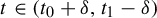 such that
$f(t)=0$
such that
$f(t)=0$
 . However, that brings us a contradiction.
Let now f be the function defined in (4.8). We will show that the set of roots of f is bounded. Observe that f can be bounded from above by

Consequently, we have
$f(\eta ) < 0$
 for
$\eta \in (-\infty , -\delta _0)\cup (\delta _0, +\infty )$
for
$\eta \in (-\infty , -\delta _0)\cup (\delta _0, +\infty )$
 , where

In particular, the set of roots of f denoted by
$Z(f)$
 is a subset of
$[-\delta _0,\delta _0]$
is a subset of
$[-\delta _0,\delta _0]$
 . Since
$Z(f)$
. Since
$Z(f)$
 is bounded and discrete, the number
$k:=\#\{ \eta \in Z(f)\ |\ \eta>0\}\in \mathbb {N}$
is bounded and discrete, the number
$k:=\#\{ \eta \in Z(f)\ |\ \eta>0\}\in \mathbb {N}$
 is well defined. Moreover, we can enumerate the elements of the set
$\{ \eta \in Z(f)\ |\ \eta>0\}=\{\eta _i\}_{i=1}^{k}$
is well defined. Moreover, we can enumerate the elements of the set
$\{ \eta \in Z(f)\ |\ \eta>0\}=\{\eta _i\}_{i=1}^{k}$
 such that
$\eta _i< \eta _{i+1}$
such that
$\eta _i< \eta _{i+1}$
 for
$i=1,\ldots k-1$
for
$i=1,\ldots k-1$
 and
and

Our aim is to prove that k is an odd number.
We will show now that if f satisfies (4.3), then
$f'(\eta _1)<0$
 . Recall that
$f(0)=\tfrac 12|q_1-q_0|^2$
. Recall that
$f(0)=\tfrac 12|q_1-q_0|^2$
 , which in the case where
$q_0\neq q_1$
, which in the case where
$q_0\neq q_1$
 , means
$f(0)>0$
, means
$f(0)>0$
 . Suppose now that
$f'(\eta _1)>0$
. Suppose now that
$f'(\eta _1)>0$
 . That would imply that there exists
$\delta>0$
. That would imply that there exists
$\delta>0$
 such that
$f(\eta )<f(\eta _1)=0$
such that
$f(\eta )<f(\eta _1)=0$
 for
$\eta \in (\eta _1-\delta , \eta _1)$
for
$\eta \in (\eta _1-\delta , \eta _1)$
 . Consequently, by the intermediate value theorem, there must exist
$\eta \in (0, \eta _1-\delta )$
. Consequently, by the intermediate value theorem, there must exist
$\eta \in (0, \eta _1-\delta )$
 such that
$f(\eta )=0$
such that
$f(\eta )=0$
 , which contradicts our assumption (4.14). Thus,
$f'(\eta _1)<0$
, which contradicts our assumption (4.14). Thus,
$f'(\eta _1)<0$
 .
.
The last step would be to show that if f satisfies (4.3), then
$f'(\eta _{k})<0$
 . Recall that
$\lim _{\eta \to +\infty }f(\eta )=-\infty $
. Recall that
$\lim _{\eta \to +\infty }f(\eta )=-\infty $
 . Suppose now that
$f'(\eta _{k})>0$
. Suppose now that
$f'(\eta _{k})>0$
 . That would imply that there exists
$\delta>0$
. That would imply that there exists
$\delta>0$
 such that for all
$\eta \in (\eta _{k}, \eta _{k}+\delta )$
such that for all
$\eta \in (\eta _{k}, \eta _{k}+\delta )$
 ,
$f(\eta )>0$
,
$f(\eta )>0$
 . Consequently, by the intermediate value theorem, there would have to exist
$\eta \in (\eta _{k}+\delta ,+\infty )$
. Consequently, by the intermediate value theorem, there would have to exist
$\eta \in (\eta _{k}+\delta ,+\infty )$
 such that
$f(\eta )=0$
such that
$f(\eta )=0$
 . However, that contradicts assumption (4.14).
Let us recall what we have learned: if f satisfies (4.3), then
$f'(\eta _1)<0$
 ,
$f'(\eta _i)$
,
$f'(\eta _i)$
 has an opposite sign than
$f'(\eta _{i+1})$
has an opposite sign than
$f'(\eta _{i+1})$
 for all
$i=1, \ldots k-1$
for all
$i=1, \ldots k-1$
 and, finally,
$f'(\eta _{k})<0$
and, finally,
$f'(\eta _{k})<0$
 . This implies that k is an odd number.
Using the same arguments, we prove that
$\#\{ \eta \in Z(f)\ |\ \eta <0\}$
 is an odd number as well.
Even though the positive Lagrangian Rabinowitz Floer homology has only one generator, the number of positive critical points of the Rabinowitz action functional corresponding to a fixed pair of endpoints
$q_0,q_1 \in \mathbb {R}^2$
 does not necessarily have to be
$1$
does not necessarily have to be
$1$
 . In fact, its cardinality depends on the value of the energy
$c>0$
. In fact, its cardinality depends on the value of the energy
$c>0$
 . As shown in Lemma 4.4, the positive critical set of the Rabinowitz action functional is in bijection with the set of positive zeroes of the corresponding function f defined in (4.8). In Figure 1, we depict the functions f corresponding to the chord endpoints
$q_0=(1,0)$
. As shown in Lemma 4.4, the positive critical set of the Rabinowitz action functional is in bijection with the set of positive zeroes of the corresponding function f defined in (4.8). In Figure 1, we depict the functions f corresponding to the chord endpoints
$q_0=(1,0)$
 ,
$q_1=(0,1)$
,
$q_1=(0,1)$
 , and three different energies
$c= \tfrac 15$
, and three different energies
$c= \tfrac 15$
 ,
$c=({1}/{10})$
,
$c=({1}/{10})$
 and
$c=({1}/{20})$
and
$c=({1}/{20})$
 . We see that the number of positive zeroes of the functions increases as the energy c decreases.
The three functions f corresponding to energy
$c=\tfrac 15$
 (blue (dark grey)),
$c=({1}/{10})$
(blue (dark grey)),
$c=({1}/{10})$
 (green (light grey)) and
$c=({1}/{20})$
(green (light grey)) and
$c=({1}/{20})$
 (magenta (medium grey)) crossing zero in exactly
$1$
(magenta (medium grey)) crossing zero in exactly
$1$
 ,
$3$
,
$3$
 and
$5$
and
$5$
 points, respectively (colour online).

Figure 1 Long description
The line graph features a horizontal x-axis ranging from 0 to approximately 23 and a vertical y-axis ranging from -10 to 5. Three distinct curves represent different energy levels.
* The blue curve, representing energy J equals 1 over 5, starts at y equals 1, peaks near x equals 3, and crosses the x-axis once before descending sharply.
* The green curve, representing energy J equals 1 over 10, follows a similar initial path but with higher peaks and deeper troughs. It crosses the x-axis three times, with peaks near x equals 3 and x equals 9, and a trough near x equals 15.
* The magenta curve, representing energy J equals 1 over 20, exhibits the highest amplitude and most frequent oscillations. It crosses the x-axis five times, with prominent peaks near x equals 3, 9, 16, and 22, and deep troughs between them.
All three curves originate from the same point on the y-axis at x equals 0 and diverge as x increases, showing a correlation between lower energy values and increased oscillatory frequency.
The following proposition shows that the number of positive critical points of the Rabinowitz action functional tends to
$\infty $
 as the energy c approaches
$0$
as the energy c approaches
$0$
 .
.
Proposition 4.9. For fixed
$q_0,q_1 \in \mathbb {R}^2$
 , we have

Proof. By Lemma 4.4, we know that for any fixed
$q_0,q_1 \in \mathbb {R}^2$
 and
$c>0$
and
$c>0$
 , we have
$ \#(\operatorname {Crit}^+ \mathcal {A}_{q_0,q_1}^{H_0-c})= \# \{ \eta>0\ |\ f(\eta )=0\}$
, we have
$ \#(\operatorname {Crit}^+ \mathcal {A}_{q_0,q_1}^{H_0-c})= \# \{ \eta>0\ |\ f(\eta )=0\}$
 , where f is the function defined in (4.8), which depends on
$q_0$
, where f is the function defined in (4.8), which depends on
$q_0$
 ,
$q_1$
,
$q_1$
 and c. We express
$q_0$
and c. We express
$q_0$
 and
$q_1$
and
$q_1$
 in polar coordinates as

Plugging this into the function f from (4.8), we obtain

Note that the function depends only on the relative angle
$\theta $
 between the two endpoints. This is not very surprising as the Hamiltonian
$H_0$
between the two endpoints. This is not very surprising as the Hamiltonian
$H_0$
 is invariant under rotations around the origin. Observe that

Consequently, we have

Note that if we assume

then

Now, exactly one of
$n,n+1$
 is even and the other is odd, so

and thus by the intermediate value theorem, there exists
$\eta \in (\pi n-\theta , \pi (n+1)-\theta )$
 such that
$f(\eta )=0$
such that
$f(\eta )=0$
 .
.
Therefore, we can estimate

The length of the interval on the right-hand side of the inequality is equal to
$({\sqrt {2}}/{\pi \sqrt {c}})\min \{r_0,r_1\}-1$
 . Since
$\lim _{c\to 0}({\sqrt {2}}/{\pi \sqrt {c}}\min \{r_0,r_1\}-1)=+\infty $
. Since
$\lim _{c\to 0}({\sqrt {2}}/{\pi \sqrt {c}}\min \{r_0,r_1\}-1)=+\infty $
 , we conclude

In Figures 2, 3 and 4, we present the plots of the Reeb chords from
$q_0=(0,1)$
 to
$q_1=(1,0)$
to
$q_1=(1,0)$
 for various energies. More precisely, the graphs depict the projections of the Reeb chords onto the plane of positions. The plots have been obtained using the formula from Lemma 4.4.
The unique Reeb chords of energy
$c=1$
 (green (light grey)),
$c=\tfrac 12$
(green (light grey)),
$c=\tfrac 12$
 (blue (dark grey)) and
$c=\tfrac 15$
(blue (dark grey)) and
$c=\tfrac 15$
 (magenta (medium grey)) (colour online).

Figure 2 Long description
The graph features a vertical y-axis ranging from -1.0 to 1.0 and a horizontal x-axis ranging from -0.5 to 1.0. All three curves originate at the point (0, 1.0) and terminate near (1.0, 0).
* The green curve (J equals 1) follows a relatively direct path, sloping downward with a slight convex bend, crossing the x-axis near 0.85 before curving upward to the endpoint.
* The blue curve (J equals 1 over 2) drops more sharply, crossing the x-axis near 0.45, reaching a trough at approximately (0.75, -0.65), and then rising steeply to the endpoint.
* The magenta curve (J equals 1 over 5) exhibits the most complex path. It initially stays higher than the others, then drops vertically near x equals 0.4, crossing the x-axis and plunging to a deep trough at approximately (0.45, -0.95). It then rises diagonally to meet the other curves at the endpoint.
The three Reeb chords of energy
$c=({1}/{10})$
 (colour online).

Figure 3 Long description
A line graph plotted on a coordinate system with x and y axes ranging from negative 1.0 to 1.0. The graph features three distinct closed loops in blue, green, and magenta.
* The blue loop is the most vertical, centered primarily in the right half of the plane. It starts near (0, 1.0), curves down through the fourth quadrant to a minimum near (0.2, negative 1.0), and returns upward.
* The green loop is elongated horizontally. It extends furthest left to approximately negative 0.9 on the x-axis in the second quadrant and furthest right to 1.0 in the fourth quadrant, crossing the y-axis near negative 0.6.
* The magenta loop is the most expansive, intersecting the other two. It reaches a peak in the second quadrant near (negative 0.5, 0.8), passes through the origin area, and curves through the first and fourth quadrants, touching the x-axis at 1.0.
All three curves originate or converge near the top point (0, 1.0) and the far right point (1.0, 0).
The five Reeb chords of energy
$c=({1}/{20})$
 . (Colour online)

Figure 4 Long description
A mathematical line graph plotted on a Cartesian coordinate system with x and y axes ranging from negative 1.0 to 1.0. The origin is at the center. Five distinct colored loops are shown.
* A dark blue loop starts at the top y-axis at 1.0, curves down through the first quadrant, and crosses the x-axis near 0.4.
* A magenta loop is oriented vertically, crossing the x-axis at approximately negative 0.3 and 0.7.
* A gold loop is oriented horizontally, crossing the y-axis at approximately 0.4 and negative 0.6.
* A teal loop forms a wide diagonal path from the upper left to the lower right.
* A green loop forms a similar diagonal path but is shifted further toward the negative x and y boundaries.
All loops are contained within the circular boundary defined by the 1.0 and negative 1.0 limits on both axes, creating a complex web of intersections across all four quadrants.
Let us analyse how the number of Reeb chords depends on the energy
$c\in \lbrace 1, \tfrac 12, \tfrac 15, ({1}/{10}), ({1}/{20})\rbrace $
 . By Lemma 4.5, we have
$\operatorname {Crit}^+\mathcal {A}_{q_0,q_1}^{H_0-c}=1$
. By Lemma 4.5, we have
$\operatorname {Crit}^+\mathcal {A}_{q_0,q_1}^{H_0-c}=1$
 for
$c \geq \tfrac 12$
for
$c \geq \tfrac 12$
 . However, from Lemma 4.4, we know that
$\operatorname {Crit}^+\mathcal {A}_{q_0,q_1}^{H_0-c}$
. However, from Lemma 4.4, we know that
$\operatorname {Crit}^+\mathcal {A}_{q_0,q_1}^{H_0-c}$
 is in bijection with the zeroes of the corresponding function f in (4.8). By (4.13), we know that

Calculating the interval for various energies, we obtain

Consequently, Figure 1 depicts the three functions f corresponding to energies
${c\in \lbrace \tfrac 15, ({1}/{10}), ({1}/{20})\rbrace }$
 on the whole interval
$[0,\delta _0]$
on the whole interval
$[0,\delta _0]$
 . Therefore, we can deduce that the plot in Figure 1 depicts all the zeros of the three functions. Hence,

From the discussion above, we know that

In other words, on each of the level sets corresponding to
$c=1$
 ,
$c=\tfrac 12$
,
$c=\tfrac 12$
 and
$c=\tfrac 15$
and
$c=\tfrac 15$
 , there is exactly one Reeb chord from
$q_0=(0,1)$
, there is exactly one Reeb chord from
$q_0=(0,1)$
 to
$q_1=(1,0)$
to
$q_1=(1,0)$
 . These Reeb chords are presented in Figure 2.
Figure 3 depicts the three Reeb chords from
$q_0=(0,1)$
 to
$q_1=(1,0)$
to
$q_1=(1,0)$
 of energy
${c=({1}/{10})}$
of energy
${c=({1}/{10})}$
 , and Figure 4 shows the five Reeb chords of energy
$c=({1}/{20})$
, and Figure 4 shows the five Reeb chords of energy
$c=({1}/{20})$
 .
.
4.3 Calculating the Maslov index
In this subsection, we will prove Theorem 1.2. Let
$H_0$
 be the Hamiltonian as in (1.1) and let
$\mathcal {H}$
be the Hamiltonian as in (1.1) and let
$\mathcal {H}$
 be the set of perturbations as defined in (1.2). By Proposition 4.2, we know that for all
$h\in \mathcal {H}$
be the set of perturbations as defined in (1.2). By Proposition 4.2, we know that for all
$h\in \mathcal {H}$
 and all pairs
$q_0,q_1\in \mathbb {R}^2$
and all pairs
$q_0,q_1\in \mathbb {R}^2$
 ,
$q_0\neq q_1$
,
$q_0\neq q_1$
 , the positive Lagrangian Rabinowitz Floer homology of the triple
$\mathrm {LRFH}_*^+(\mathcal {A}^{H_0-h}_{q_0,q_1})$
, the positive Lagrangian Rabinowitz Floer homology of the triple
$\mathrm {LRFH}_*^+(\mathcal {A}^{H_0-h}_{q_0,q_1})$
 is well defined and isomorphic to
$\mathrm {LRFH}_*^+(\mathcal {A}^{H_0-c}_{q_0,q_1})$
is well defined and isomorphic to
$\mathrm {LRFH}_*^+(\mathcal {A}^{H_0-c}_{q_0,q_1})$
 for any
$c>0$
for any
$c>0$
 . However, by Proposition 4.3, we know that if
$c\geq \tfrac 12|q_0||q_1|$
. However, by Proposition 4.3, we know that if
$c\geq \tfrac 12|q_0||q_1|$
 , then
$\operatorname {Crit}^+\mathcal {A}^{H_0-c}_{q_0,q_1}$
, then
$\operatorname {Crit}^+\mathcal {A}^{H_0-c}_{q_0,q_1}$
 has only one element. Consequently,
$\mathrm { LRFH}_*^+(\mathcal {A}^{H_0-c}_{q_0,q_1})$
has only one element. Consequently,
$\mathrm { LRFH}_*^+(\mathcal {A}^{H_0-c}_{q_0,q_1})$
 has only one generator and its boundary operator is
$0$
has only one generator and its boundary operator is
$0$
 . Therefore, to calculate the positive Lagrangian Rabinowitz Floer homology explicitly, what is left to do is to calculate the Maslov index of
$(v,\eta )\in \operatorname {Crit}^+\mathcal {A}^{H_0-c}_{q_0,q_1}$
. Therefore, to calculate the positive Lagrangian Rabinowitz Floer homology explicitly, what is left to do is to calculate the Maslov index of
$(v,\eta )\in \operatorname {Crit}^+\mathcal {A}^{H_0-c}_{q_0,q_1}$
 .
.
Lemma 4.10. For
$c>0$
 , define a Hamiltonian
$H_c:T^*\mathbb {R}^2\to \mathbb {R}$
, define a Hamiltonian
$H_c:T^*\mathbb {R}^2\to \mathbb {R}$
 as
as

Let
$H_0$
 be the Hamiltonian as in (1.1) and let
$\varphi _\delta $
be the Hamiltonian as in (1.1) and let
$\varphi _\delta $
 be a diffeomorphism of
$T^*\mathbb {R}^2$
be a diffeomorphism of
$T^*\mathbb {R}^2$
 defined
$\varphi _\delta (q,p):=(\sqrt {\delta }q,({1}/{\sqrt {\delta }})p)$
defined
$\varphi _\delta (q,p):=(\sqrt {\delta }q,({1}/{\sqrt {\delta }})p)$
 . Then,

Proof. First, observe that
$\varphi $
 preserves the standard symplectic form, so it is a symplectomorphism. Moreover, the Hamiltonians satisfy the relation
$H_\delta =\delta H_0\circ \varphi _\delta $
preserves the standard symplectic form, so it is a symplectomorphism. Moreover, the Hamiltonians satisfy the relation
$H_\delta =\delta H_0\circ \varphi _\delta $
 ; thus,

Now,
$(v,\eta )\in \operatorname {Crit} \mathcal {A}_{q_0,q_1}^{H_\delta -1}$
 if and only if
$v(i)=q_i$
if and only if
$v(i)=q_i$
 for
$i=1,2$
for
$i=1,2$
 ,
$v([0,1])\subseteq H_\delta ^{-1}(1)$
,
$v([0,1])\subseteq H_\delta ^{-1}(1)$
 and
$\partial _t v=\eta X_{H_\delta }(v)$
and
$\partial _t v=\eta X_{H_\delta }(v)$
 . Naturally, the first two conditions are trivially equivalent. It suffices to verify that

Lemma 4.11. Let
$\{H_\delta \}_{\delta>0}$
 be the family of Hamiltonians defined in (4.15). Let
${H_{{\bullet }}:T^*\mathbb {R}^2\to \mathbb {R}}$
be the family of Hamiltonians defined in (4.15). Let
${H_{{\bullet }}:T^*\mathbb {R}^2\to \mathbb {R}}$
 be the kinetic Hamiltonian
$H_{{\bullet }}(q,p):=\tfrac 12|p|^2$
be the kinetic Hamiltonian
$H_{{\bullet }}(q,p):=\tfrac 12|p|^2$
 . Fix
$q_0,q_1\in \mathbb {R}^2$
. Fix
$q_0,q_1\in \mathbb {R}^2$
 ,
$q_0\neq q_1$
,
$q_0\neq q_1$
 . Then, for
$\delta <\sqrt {{2}/{(|q_0||q_1|)}}$
. Then, for
$\delta <\sqrt {{2}/{(|q_0||q_1|)}}$
 (in the case where
$q_0=0$
(in the case where
$q_0=0$
 or
$q_1=0$
or
$q_1=0$
 for any
$\delta>0$
for any
$\delta>0$
 ), we have
$\#\operatorname {Crit}^+\mathcal {A}^{H_\delta -1}_{q_0,q_1}=1$
), we have
$\#\operatorname {Crit}^+\mathcal {A}^{H_\delta -1}_{q_0,q_1}=1$
 and the family of Reeb chords
$(v_\delta ,\eta _\delta )\in \operatorname {Crit}^+\mathcal {A}^{H_\delta -1}_{q_0,q_1}$
and the family of Reeb chords
$(v_\delta ,\eta _\delta )\in \operatorname {Crit}^+\mathcal {A}^{H_\delta -1}_{q_0,q_1}$
 satisfies

Proof. Using Lemma 4.10, we know that for every
$\delta>0$
 , there is a bijection between
$\operatorname {Crit}^+\mathcal {A}_{q_0,q_1}^{H_\delta -1}$
, there is a bijection between
$\operatorname {Crit}^+\mathcal {A}_{q_0,q_1}^{H_\delta -1}$
 and
$\operatorname {Crit}^+ \mathcal {A}_{\varphi _\delta (q_0),\varphi _\delta (q_1)}^{H_0-({1}/{\delta })}$
and
$\operatorname {Crit}^+ \mathcal {A}_{\varphi _\delta (q_0),\varphi _\delta (q_1)}^{H_0-({1}/{\delta })}$
 . However, by Proposition 4.3, we know that for
$|\varphi _\delta (q_0)||\varphi _\delta (q_1)|=\delta |q_0||q_1|\leq ({2}/{\delta })$
. However, by Proposition 4.3, we know that for
$|\varphi _\delta (q_0)||\varphi _\delta (q_1)|=\delta |q_0||q_1|\leq ({2}/{\delta })$
 , we have
$1=\# \operatorname {Crit}^+ \mathcal {A}_{\varphi _\delta (q_0),\varphi _\delta (q_1)}^{H_0-({1}/{\delta })}=\# \operatorname {Crit}^+ \mathcal {A}_{q_0,q_1}^{H_\delta -1}$
, we have
$1=\# \operatorname {Crit}^+ \mathcal {A}_{\varphi _\delta (q_0),\varphi _\delta (q_1)}^{H_0-({1}/{\delta })}=\# \operatorname {Crit}^+ \mathcal {A}_{q_0,q_1}^{H_\delta -1}$
 . Consequently, for every
$\delta <\sqrt {{2}/{(|q_0||q_1|)}}$
. Consequently, for every
$\delta <\sqrt {{2}/{(|q_0||q_1|)}}$
 (or in the case where either
$q_0$
(or in the case where either
$q_0$
 or
$q_1$
or
$q_1$
 are zero for any
$\delta>0$
are zero for any
$\delta>0$
 ), there is a unique solution
$(v_\delta ,\eta _\delta )\in \operatorname {Crit}^+ \mathcal {A}_{q_0,q_1}^{H_\delta -1}$
), there is a unique solution
$(v_\delta ,\eta _\delta )\in \operatorname {Crit}^+ \mathcal {A}_{q_0,q_1}^{H_\delta -1}$
 .
.
Having established that
$(v_\delta ,\eta _\delta )\in \operatorname {Crit}^+\mathcal {A}^{H_\delta -1}_{q_0,q_1}$
 is uniquely defined for small enough
$\delta $
is uniquely defined for small enough
$\delta $
 , we can use the function f from Lemma 4.4 to estimate
$\eta _\delta $
, we can use the function f from Lemma 4.4 to estimate
$\eta _\delta $
 . We simply need to map
$(c,q_0,q_1,\eta )\mapsto (({1}/{\delta }), \sqrt {\delta }q_0, \sqrt {\delta }q_1, \delta \eta )$
. We simply need to map
$(c,q_0,q_1,\eta )\mapsto (({1}/{\delta }), \sqrt {\delta }q_0, \sqrt {\delta }q_1, \delta \eta )$
 to obtain that
$\eta _\delta $
to obtain that
$\eta _\delta $
 is the unique positive root of the function:

This way, we know that
$(v_\delta ,\eta _\delta )\in \operatorname {Crit}^+\mathcal {A}^{H_\delta -1}_{q_0,q_1}$
 if and only if
$g_\delta (\eta _\delta )=0$
if and only if
$g_\delta (\eta _\delta )=0$
 .
.
By (4.16), we can use the Taylor expansion to obtain the following estimate:

which directly gives us
$\lim _{\delta \to 0}\eta _\delta =({1}/{\sqrt {2}})|q_1-q_0|$
 .
.
To show the convergence of
$v_\delta $
 , we again use Lemma 4.4 to present the equation for
$v_\delta $
, we again use Lemma 4.4 to present the equation for
$v_\delta $
 explicitly. By Lemma 4.10, it suffices to just use the mapping
$(q_0,q_1,\eta )\mapsto (\sqrt {\delta }q_0, \sqrt {\delta }q_1, \delta \eta )$
explicitly. By Lemma 4.10, it suffices to just use the mapping
$(q_0,q_1,\eta )\mapsto (\sqrt {\delta }q_0, \sqrt {\delta }q_1, \delta \eta )$
 in the formula for
$v_\delta $
in the formula for
$v_\delta $
 from Lemma 4.4 to obtain

Consider the functions
$t \mapsto R(t\delta \eta _\delta )$
 and
$t\mapsto R((1-t)\delta \eta _\delta )$
and
$t\mapsto R((1-t)\delta \eta _\delta )$
 on the interval
$[0,1]$
on the interval
$[0,1]$
 . Since
$\lim _{\delta \to 0}\delta \eta _\delta =0$
. Since
$\lim _{\delta \to 0}\delta \eta _\delta =0$
 , we have the uniform convergence
$\lim _{\delta \to 0}R(t\delta \eta _\delta )= \lim _{\delta \to 0}R((1-t)\delta \eta _\delta )=\operatorname {Id}$
, we have the uniform convergence
$\lim _{\delta \to 0}R(t\delta \eta _\delta )= \lim _{\delta \to 0}R((1-t)\delta \eta _\delta )=\operatorname {Id}$
 . Consequently,

A straightforward calculation shows that
$(v_0,\eta _0)$
 with
$\eta _0:=({1}/{\sqrt {2}})|q_1-q_0|$
with
$\eta _0:=({1}/{\sqrt {2}})|q_1-q_0|$
 is the unique element of
$\operatorname {Crit}^+\mathcal {A}^{H_{{\bullet }}-1}_{q_0,q_1}$
is the unique element of
$\operatorname {Crit}^+\mathcal {A}^{H_{{\bullet }}-1}_{q_0,q_1}$
 .
.
Proof of Theorem 1.2
By Proposition 4.2, we know that for all
$h\in \mathcal {H}$
 and all
$q_0,q_1\in \mathbb {R}^2$
and all
$q_0,q_1\in \mathbb {R}^2$
 with
$q_0\neq q_1$
with
$q_0\neq q_1$
 , the positive Lagrangian Rabinowitz Floer homology
$\mathrm {LRFH}_*^+(\mathcal {A}^{H_0-h}_{q_0,q_1})$
, the positive Lagrangian Rabinowitz Floer homology
$\mathrm {LRFH}_*^+(\mathcal {A}^{H_0-h}_{q_0,q_1})$
 is well defined and isomorphic to
$\mathrm {LRFH}_*^+(\mathcal {A}^{H_0-c}_{q_0,q_1})$
is well defined and isomorphic to
$\mathrm {LRFH}_*^+(\mathcal {A}^{H_0-c}_{q_0,q_1})$
 for any
$c>0$
for any
$c>0$
 . However, by Proposition 4.3, we know that if
$c\geq |q_0||q_1|/2$
. However, by Proposition 4.3, we know that if
$c\geq |q_0||q_1|/2$
 , then
$\operatorname {Crit}^+\mathcal {A}^{H_0-c}_{q_0,q_1}$
, then
$\operatorname {Crit}^+\mathcal {A}^{H_0-c}_{q_0,q_1}$
 has only one element. Consequently,
$\mathrm { LRFH}_*^+(\mathcal {A}^{H_0-c}_{q_0,q_1})$
has only one element. Consequently,
$\mathrm { LRFH}_*^+(\mathcal {A}^{H_0-c}_{q_0,q_1})$
 has only one generator and its boundary operator is
$0$
has only one generator and its boundary operator is
$0$
 . It remains to calculate the Maslov index of this generator.
Let
$\{H_\delta \}_{\delta>0}$
 be the family of Hamiltonians defined in (4.15) and let
$\varphi _\delta $
be the family of Hamiltonians defined in (4.15) and let
$\varphi _\delta $
 be the family of symplectomorphisms defined by
$\varphi _\delta (q,p):=(({1}/{\sqrt {\delta }})q,\sqrt {\delta }p)$
be the family of symplectomorphisms defined by
$\varphi _\delta (q,p):=(({1}/{\sqrt {\delta }})q,\sqrt {\delta }p)$
 . By Lemma 4.10, for every
$c>0$
. By Lemma 4.10, for every
$c>0$
 , we have

Since the Maslov index is invariant under symplectomorphisms, we get

Therefore, it suffices to calculate
$\mu ^{\mathrm {tr}}( v_\delta ({\cdot }/{\eta _\delta }))$
 of the unique
$(v_\delta , \eta _\delta )\in \operatorname {Crit}^+\mathcal {A}^{H_\delta -1}_{q_0,q_1}$
of the unique
$(v_\delta , \eta _\delta )\in \operatorname {Crit}^+\mathcal {A}^{H_\delta -1}_{q_0,q_1}$
 for
$\delta>0$
for
$\delta>0$
 small enough.
Denote by
$H_{{\bullet }}$
 the kinetic Hamiltonian
$H_{{\bullet }}(q,p):=\tfrac 12|p|^2$
the kinetic Hamiltonian
$H_{{\bullet }}(q,p):=\tfrac 12|p|^2$
 and let
$(v_0,\eta _0)$
and let
$(v_0,\eta _0)$
 be the unique element of
$\operatorname {Crit}^+\mathcal {A}^{H_{{\bullet }}-1}_{q_0,q_1}$
be the unique element of
$\operatorname {Crit}^+\mathcal {A}^{H_{{\bullet }}-1}_{q_0,q_1}$
 as in (4.17). By Lemma 4.11, we know that
$\lim _{\delta \to 0}(v_\delta , \eta _\delta )=(v_0,\eta _0)$
as in (4.17). By Lemma 4.11, we know that
$\lim _{\delta \to 0}(v_\delta , \eta _\delta )=(v_0,\eta _0)$
 . Continuity of the Maslov index and Example 2.3 implies

for small enough
$\delta>0$
 . Consequently, by Proposition 4.2 for all
$h\in \mathcal {H}$
. Consequently, by Proposition 4.2 for all
$h\in \mathcal {H}$
 , all
$q_0,q_1\in \mathbb {R}^2$
, all
$q_0,q_1\in \mathbb {R}^2$
 and for
$c>|q_0||q_1|/2$
and for
$c>|q_0||q_1|/2$
 big enough, we obtain

This concludes the proof of Theorem 1.2.
5 Non-compactly supported potential
The aim of this section will be to prove Proposition 1.3. Let
$H_0: T^*\mathbb {R}^2 \to \mathbb {R}$
 be the quadratic Hamiltonian defined in (1.1) and let
$V:\mathbb {R}^2 \to \mathbb {R}$
be the quadratic Hamiltonian defined in (1.1) and let
$V:\mathbb {R}^2 \to \mathbb {R}$
 be the potential function as in Proposition 1.3.

Then,

The first step to prove Proposition 1.3 is to show that for positive energy
$c>0$
 and a fixed pair
$q_0,q_1\in \mathbb {R}^2$
and a fixed pair
$q_0,q_1\in \mathbb {R}^2$
 , all Reeb chords on
$H^{-1}(c)$
, all Reeb chords on
$H^{-1}(c)$
 between the Lagrangians
$T^*_{q_0}\mathbb {R}^2$
between the Lagrangians
$T^*_{q_0}\mathbb {R}^2$
 and
$T^*_{q_1}\mathbb {R}^2$
and
$T^*_{q_1}\mathbb {R}^2$
 are contained in a compact subset of
$T^*\mathbb {R}^2$
are contained in a compact subset of
$T^*\mathbb {R}^2$
 .
.
Proposition 5.1. Let
$H: T^*\mathbb {R}^2 \to \mathbb {R}$
 be the Hamiltonian defined in (5.1). Fix
$c>0$
be the Hamiltonian defined in (5.1). Fix
$c>0$
 and
$q_0,q_1 \in \mathbb {R}^2$
and
$q_0,q_1 \in \mathbb {R}^2$
 and let
$\mathcal {A}^{H-c}_{q_0,q_1}:\mathscr {H}_{q_0,q_1}\times \mathbb {R} \to \mathbb {R}$
and let
$\mathcal {A}^{H-c}_{q_0,q_1}:\mathscr {H}_{q_0,q_1}\times \mathbb {R} \to \mathbb {R}$
 be the corresponding action functional. Then, the critical set
$\operatorname {Crit} \mathcal {A}^{H-c}_{q_0,q_1}$
be the corresponding action functional. Then, the critical set
$\operatorname {Crit} \mathcal {A}^{H-c}_{q_0,q_1}$
 is bounded in
$L^\infty $
is bounded in
$L^\infty $
 .
.
Proof. By an argument similar to the one in the proof of Lemma 3.2, it suffices to show that the set

is compact. By (5.2), we have that

For
$(r, \theta , p_r, p_\theta ) \in H^{-1}(c)\cap \{\{H, r\}=0\}$
 , we have


Consequently, by our assumption on the potential function V, if
$\alpha>2$
 and
$a>0$
and
$a>0$
 , then for
$(r, \theta , p_r, p_\theta ) \in H^{-1}(c)\cap \{\{H, r\}=0\}$
, then for
$(r, \theta , p_r, p_\theta ) \in H^{-1}(c)\cap \{\{H, r\}=0\}$
 such that

However, if
$\alpha = 2$
 and
$a\in (0 ,({c^2}/{4}))$
and
$a\in (0 ,({c^2}/{4}))$
 , then for
$(r, \theta , p_r, p_\theta ) \in H^{-1}(c)\cap \{\{H, r\}=0\}$
, then for
$(r, \theta , p_r, p_\theta ) \in H^{-1}(c)\cap \{\{H, r\}=0\}$
 such that

Consequently, in both cases, the set

is bounded in r and for every
$(v, \eta ) \in \operatorname {Crit} \mathcal {A}^{H-c}_{q_0,q_1}$
 , we have

By an argument similar to the one presented in the Lemma 3.2, we obtain that
$p_r\circ v$
 and
$p_\theta \circ v$
and
$p_\theta \circ v$
 are also uniformly bounded in the following way:

Remark 5.2. Note that the assertions of Proposition 5.1 hold true also for the potential V satisfying
$V(r,\theta ) \leq ({a}/{r^2})$
 and
$({\partial V}/{\partial r}) \geq -({2 a}/{r^3})$
and
$({\partial V}/{\partial r}) \geq -({2 a}/{r^3})$
 for
$r>r_0$
for
$r>r_0$
 and
$a \in [({c^2}/{4}), ({c^2}/{2}))$
and
$a \in [({c^2}/{4}), ({c^2}/{2}))$
 . However, we were unable to prove Proposition 1.3 for this class of potentials and that is why we restrict ourselves to
$a < ({c^2}/{4})$
. However, we were unable to prove Proposition 1.3 for this class of potentials and that is why we restrict ourselves to
$a < ({c^2}/{4})$
 .
.
Now, we would like to change the Hamiltonian H by multiplying the potential function V with a compactly supported function
$\varphi : T^*\mathbb {R}^2 \to [0,1]$
 in the following way:

The associated Hamiltonian vector field is

If we choose
$\varphi $
 such that for all the Reeb chords
$(v,\eta ) \in \operatorname {Crit} \mathcal {A}^{H-c}_{q_0,q_1}$
such that for all the Reeb chords
$(v,\eta ) \in \operatorname {Crit} \mathcal {A}^{H-c}_{q_0,q_1}$
 , we would have
$v([0,1]) \subseteq \varphi ^{-1}(1)$
, we would have
$v([0,1]) \subseteq \varphi ^{-1}(1)$
 , then
$\operatorname {Crit}(\mathcal {A}^{H-c}_{q_0,q_1}) \subseteq \operatorname {Crit}(\mathcal {A}^{H_1-c}_{q_0,q_1})$
, then
$\operatorname {Crit}(\mathcal {A}^{H-c}_{q_0,q_1}) \subseteq \operatorname {Crit}(\mathcal {A}^{H_1-c}_{q_0,q_1})$
 . In fact, we would like to choose
$\varphi $
. In fact, we would like to choose
$\varphi $
 such that
$\operatorname {Crit}(\mathcal {A}^{H_1-c}_{q_0,q_1})= \operatorname {Crit}(\mathcal {A}^{H-c}_{q_0,q_1})$
such that
$\operatorname {Crit}(\mathcal {A}^{H_1-c}_{q_0,q_1})= \operatorname {Crit}(\mathcal {A}^{H-c}_{q_0,q_1})$
 .
.
Let
$\chi :\mathbb {R}\to [0,1]$
 be a smooth function such that
$-2<\chi '< 0$
be a smooth function such that
$-2<\chi '< 0$
 on
$[0,1]$
on
$[0,1]$
 and
and


Note that in both cases,
$\alpha> 2$
 and
$\alpha = 2$
and
$\alpha = 2$
 , we have
$\beta> 0$
, we have
$\beta> 0$
 . In the latter case, this follows from the assumption that
$a < ({c^2}/{4})$
. In the latter case, this follows from the assumption that
$a < ({c^2}/{4})$
 .
.
This way, we have

We will show that for a function
$\varphi $
 defined as in (5.7), we have

The first step would be to show that
$\varphi $
 has compact support.
Lemma 5.3. The function
$\varphi : T^*\mathbb {R}^2\to \mathbb {R}$
 defined as in (5.7) has compact support.
Proof. By (5.7) and (5.10), we have

Since both of the sets on the right-hand side are compact, their intersection is compact, so
$\operatorname {supp}\varphi $
 is compact as a closed subset of a compact set.
Lemma 5.4. Let
$V:\mathbb {R}^2\to \mathbb {R}$
 be a potential function as in Proposition 1.3 and let
$\varphi $
be a potential function as in Proposition 1.3 and let
$\varphi $
 be the corresponding function defined in (5.7). Then,
$\varphi V+c \in \mathcal {H}$
be the corresponding function defined in (5.7). Then,
$\varphi V+c \in \mathcal {H}$
 .
.
Proof. First, observe that

and hence,
$d(\varphi V)\in C_c^\infty (T^*\mathbb {R}^2)$
 . However, by definition,

Since by assumption, the functions V,
$\chi _0$
 ,
$\chi _1$
,
$\chi _1$
 and
$-\chi '$
and
$-\chi '$
 are non-negative, it suffices to prove that
$dH_0(p\partial _p)\geq 0$
are non-negative, it suffices to prove that
$dH_0(p\partial _p)\geq 0$
 on
$\chi _1^{-1}((0,1))$
on
$\chi _1^{-1}((0,1))$
 . Note that on
$\chi _1^{-1}((0,1))$
. Note that on
$\chi _1^{-1}((0,1))$
 , we have
$H_0> \sup V+c$
, we have
$H_0> \sup V+c$
 . Combining that with (3.4), we can calculate that on
$\chi _1^{-1}((0,1))$
. Combining that with (3.4), we can calculate that on
$\chi _1^{-1}((0,1))$
 , we have

Now that we have proven that
$\varphi $
 as in (5.7) is an eligible candidate, we will continue with the proof of Proposition 1.3. However, we will first start with the proof of a series of lemmas.
Lemma 5.5. Let H be the Hamiltonian defined in (5.1) and let
$\varphi $
 be the function defined in (5.7). Then,

Proof. By definition of H, we have

so
$H^{-1}(c) \subseteq H_0^{-1}((-\infty , \sup V+c])$
 . However, by Proposition 5.1 for every
$(v,\eta )\in \operatorname {Crit}\mathcal {A}^{H-c}_{q_0,q_1}$
. However, by Proposition 5.1 for every
$(v,\eta )\in \operatorname {Crit}\mathcal {A}^{H-c}_{q_0,q_1}$
 , we have

Lemma 5.6. Let
$H_1$
 be the Hamiltonian defined in (5.5) and let
$\varphi $
be the Hamiltonian defined in (5.5) and let
$\varphi $
 be the function defined in (5.7). Then,

Proof. First, observe that
$H_1|_{\varphi ^{-1}(0)}=H_0$
 , so by (3.1), we have

However, if
$x \in \chi _1^{-1}([0,1))$
 , then
$H_0(x)>\sup V+c$
, then
$H_0(x)>\sup V+c$
 and
and

Hence,
$\chi _1^{-1}((0,1])\cap H_1^{-1}(c)=\emptyset $
 . Therefore, we can restrict ourselves to the analysis of the set
$\chi _0^{-1}((0,1))$
. Therefore, we can restrict ourselves to the analysis of the set
$\chi _0^{-1}((0,1))$
 , that is, when
$ R_1 < r < R_1+({1}/{\beta })$
, that is, when
$ R_1 < r < R_1+({1}/{\beta })$
 .
.
Let us calculate

In particular, by (5.2), we have

By assumption,
$V, \chi \geq 0$
 and
$\chi '\leq 0$
and
$\chi '\leq 0$
 ; thus,
$\{H_1,r\}=0$
; thus,
$\{H_1,r\}=0$
 implies
$p_r=0$
implies
$p_r=0$
 .
.
Consider now
$(r, \theta , p_r, p_\theta ) \in H_1^{-1}(0)\cap (\{H_1, r\})^{-1}(0)$
 . Then,

Again, since by assumption,
$V, \chi \geq 0$
 and
$\chi '\leq 0$
and
$\chi '\leq 0$
 , then
$1-\chi _0\chi _1'V\geq 1$
, then
$1-\chi _0\chi _1'V\geq 1$
 and
$\{H_1,\{H_1,r\}\}$
and
$\{H_1,\{H_1,r\}\}$
 has the same sign as

Furthermore, since by assumption,
$V, \chi _0, p_\theta \geq 0$
 and
$\chi _1' \leq 0$
and
$\chi _1' \leq 0$
 , consequently,
$-({p_\theta ^2}/{r^3}) \chi _0\chi _1'V \geq 0$
, consequently,
$-({p_\theta ^2}/{r^3}) \chi _0\chi _1'V \geq 0$
 and we can estimate (5.11) from below by

We will show that (5.12) is positive for both cases
$\alpha>2$
 and
$\alpha =2$
and
$\alpha =2$
 .
.
Case
$\alpha>2$
 . By (5.8), we have that
$r> R_1 \geq ({8a\alpha }/{c^2})^{{1}/{\alpha -2}}$
. By (5.8), we have that
$r> R_1 \geq ({8a\alpha }/{c^2})^{{1}/{\alpha -2}}$
 , so
$({c^2}/{4r^3})>({2a\alpha }/{r^{\alpha +1}})$
, so
$({c^2}/{4r^3})>({2a\alpha }/{r^{\alpha +1}})$
 . However,
$r < R_1+({1}/{\beta })=R_1({\alpha }/{\alpha -2})$
. However,
$r < R_1+({1}/{\beta })=R_1({\alpha }/{\alpha -2})$
 . Combining that with the assumptions on the potential V and the fact that
$-2\leq \chi '\leq 0$
. Combining that with the assumptions on the potential V and the fact that
$-2\leq \chi '\leq 0$
 and
$0\leq \chi \leq 1$
and
$0\leq \chi \leq 1$
 , we obtain

Case
$\alpha =2$
 . By (5.4), (5.8) and (5.10), we have


Therefore, by (5.9) and (5.10), we obtain

Consequently, in both cases, we have

which proves the claim.
Proof of Proposition 1.3
By Lemma 5.5, we know that

However, by definition,
$H_1|_{\varphi ^{-1}(1)}=H|_{\varphi ^{-1}(1)}$
 . Thus,
$\operatorname {Crit}\mathcal {A}^{H-c}_{q_0,q_1} \subseteq \operatorname {Crit}\mathcal {A}^{H_1-c}_{q_0,q_1}$
. Thus,
$\operatorname {Crit}\mathcal {A}^{H-c}_{q_0,q_1} \subseteq \operatorname {Crit}\mathcal {A}^{H_1-c}_{q_0,q_1}$
 .
.
Nevertheless, by an argument as in the proof of Proposition 5.1, we know that for all
$(v,\eta )\in \operatorname {Crit}\mathcal {A}^{H_1-c}_{q_0,q_1}$
 , if
$\max _{t\in [0,1]}r \circ v = r\circ v(t_0)$
, if
$\max _{t\in [0,1]}r \circ v = r\circ v(t_0)$
 , then

Moreover, by Lemma 5.6, we know that

Consequently, for all
$(v,\eta )\in \operatorname {Crit}\mathcal {A}^{H_1-c}_{q_0,q_1}$
 , we have
$\max r\circ v \leq R_1$
, we have
$\max r\circ v \leq R_1$
 . In other words, for all
$(v,\eta )\in \operatorname {Crit}\mathcal {A}^{H_1-c}_{q_0,q_1}$
. In other words, for all
$(v,\eta )\in \operatorname {Crit}\mathcal {A}^{H_1-c}_{q_0,q_1}$
 , we have

However, the Hamiltonians satisfy

Consequently, for all
$(v,\eta )\in \operatorname {Crit}\mathcal {A}^{H_1-c}_{q_0,q_1}$
 , we have

However, on
$\varphi ^{-1}(1)$
 , the two Hamiltonians
$H_1$
, the two Hamiltonians
$H_1$
 and H coincide. Therefore,
$\operatorname {Crit} \mathcal {A}^{H-c}_{q_0,q_1} = \operatorname {Crit} \mathcal {A}^{H_1-c}_{q_0,q_1}$
and H coincide. Therefore,
$\operatorname {Crit} \mathcal {A}^{H-c}_{q_0,q_1} = \operatorname {Crit} \mathcal {A}^{H_1-c}_{q_0,q_1}$
 .
.
Acknowledgements
K.C. is funded by the Deutsche Forschungsgemeinschaft (DFG, German Research Foundation)—541525489. U.F. is funded by the Deutsche Forschungsgemeinschaft (DFG, German Research Foundation)—541525489. E.M. is funded by the Catalan Institution for Research and Advanced Studies via an ICREA Academia Prize 2021 and by the Alexander Von Humboldt Foundation via a Friedrich Wilhelm Bessel Research Award. She is also supported by the Spanish State Research Agency, through the Severo Ochoa and María de Maeztu Program for Centers and Units of Excellence in R&D (project CEX2020-001084-M), by the AGAUR project 2021 SGR 00603 and by the project ‘Computational, dynamical and geometrical complexity in fluid dynamics’, Ayudas Fundación BBVA a Proyectos de Investigación Científica 2021. E.M. and J.W. are partially supported by the Spanish State Research Agency grants reference PID2019-103849GB-I00 of AEI/10.13039/501100011033 and PID2023-146936NB-I00 funded by MICIU/AEI/10.13039/501100011033 and, by ERDF/EU. J.W.’s postdoctoral contract at UPC was financed under the project ‘Computational, dynamical and geometrical complexity in fluid dynamics’, Ayudas Fundación BBVA a Proyectos de Investigación Científica 2021. Her postdoctoral position in Augsburg is supported by the Deutsche Forschungsgemeinschaft (DFG, German Research Foundation) via the grant ‘Himmelsmechanik, Hydrodynamik und Turing-Maschinen’—541525489.

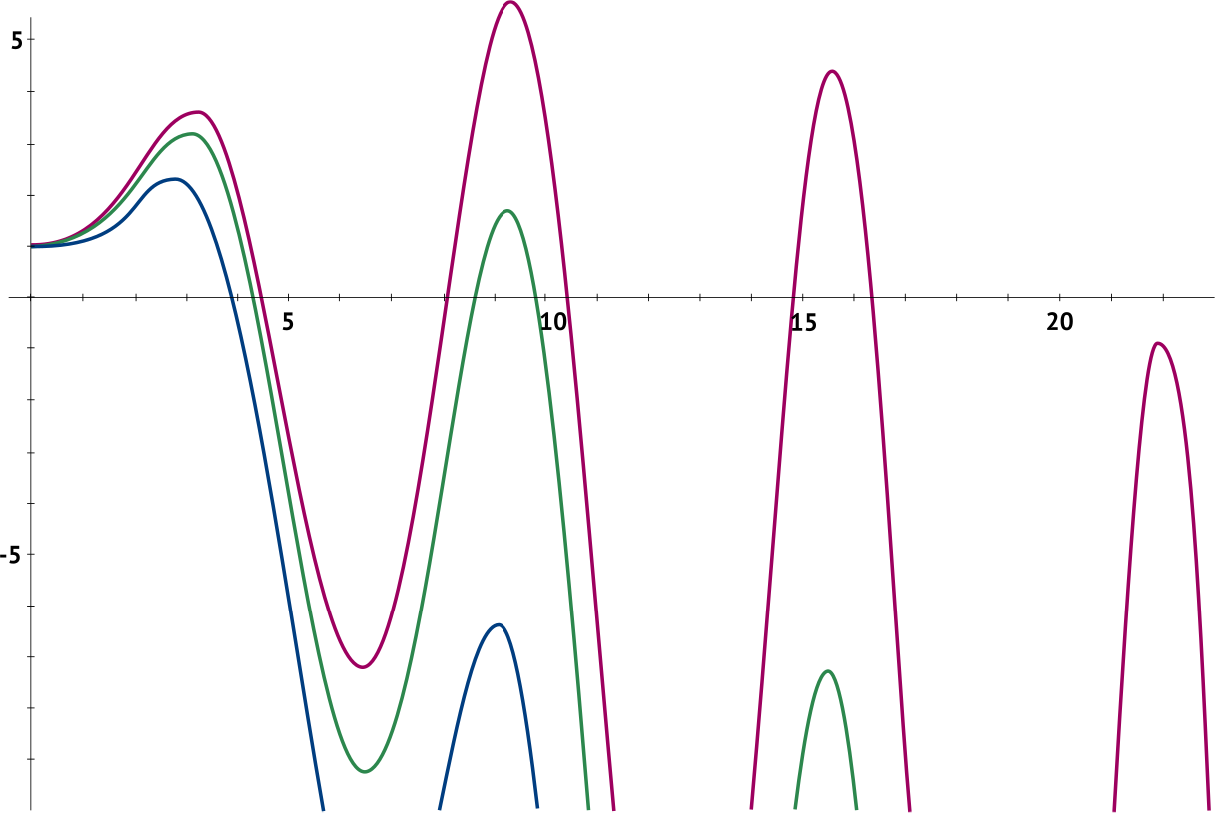


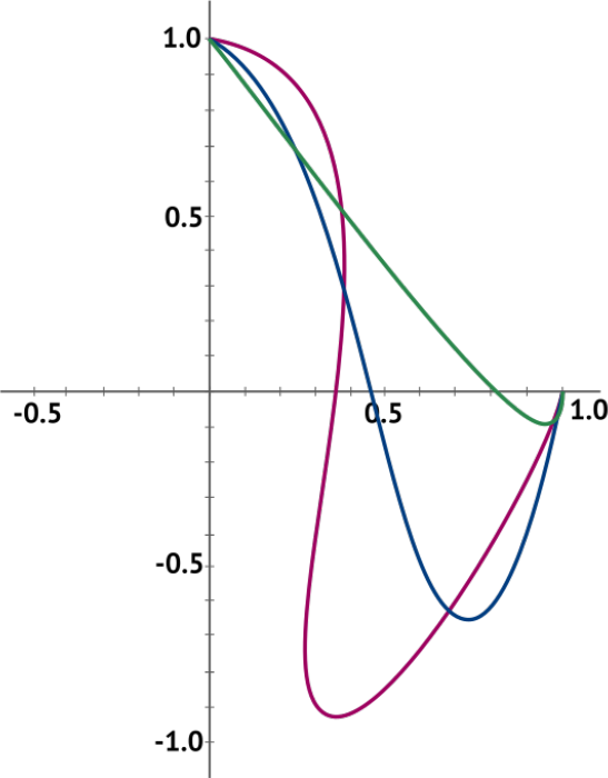


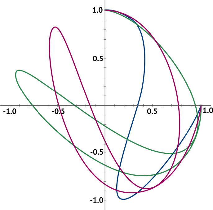


 Open access