

1. Introduction
Most Arctic and Antarctic coastal polynyas are latent-heat polynyas, which are formed by the combination of divergent sea-ice motion due to winds and/or oceanic currents and latent heat released into the water during ice formation (Reference Morales Maqueda, Willmott and BiggsMorales Maqueda and others, 2004). Under winter conditions, open water in coastal polynyas tends to freeze rapidly. Thus, most of the polynya area is covered with thin ice (i.e. frazil, grease, nilas, pancake ice, etc.) in winter, with a tentative open-water area along the coastline or landward edge of the polynya (Reference PeasePease, 1987). The region of newly formed thin ice may extend up to and in excess of 100 km from the coast in places (Reference Smith, Muench and PeaseSmith and others, 1990). During freeze-up, thin-ice areas may also exist in the marginal ice zone (MIZ). Coastal polynyas, leads and MIZ have large spatial and temporal variability. Moreover, in winter, heat loss is one to two orders of magnitude larger over thin-ice areas than over thicker ice regions (Reference MaykutMaykut, 1978). Most of the heat loss to the atmosphere is balanced by sea-ice production, so these thin-ice regions are important as sites of high sea-ice production (Gordon and Comiso, 1988). Therefore, gaining better information on the spatio-temporal distribution of thin sea ice and its variability is a key to more accurate modeling of ocean–atmosphere heat fluxes, rates of ice production and salt flux (Reference Cougnon and MeijersCougnon and others, 2013).
The most effective, and indeed only practical, means of observing thin sea-ice distribution on large scales is satellite remote sensing. Passive microwave (PMW) techniques in particular have the potential to estimate thin-ice thickness over the entire polar oceans on a daily to twice-daily basis regardless of darkness or cloud cover. Detection of thin-ice areas from satellite PMW data and the subsequent estimation of sea-ice production through the calculation of surface heat fluxes have been proven to be effective techniques (Reference Martin, Drucker, Kwok and HoltMartin and others, 2004; Reference Tamura, Ohshima and NihashiTamura and others, 2008, Reference Tamura and Ohshima2011; Reference Nihashi, Ohshima, Tamura, Fukamachi and SaitohNihashi and others, 2009; Reference Drucker, Martin and KwokDrucker and others, 2011).
With these factors in mind, an algorithm was developed to give large-scale information on thin-ice thickness using satellite PMW data from the Special Sensor Microwave/ Imager (SSM/I: 1992–present) and Advanced Microwave Scanning Radiometer–Earth Observing System (AMSR-E: 2002–11; Reference Tamura, Ohshima, Markus, Cavalieri, Nihashi and HirasawaTamura and others, 2007; Reference Nihashi, Ohshima, Tamura, Fukamachi and SaitohNihashi and others, 2009; Reference Tamura and OhshimaTamura and Ohshima, 2011; Iwamoto and others, 2013). This algorithm is based on the fact that although the microwave penetration depth of bare (thin) sea ice is in the order of 0.1 m at most (Ulaby and others, 1982), microwave brightness temperatures (TBs) at the frequencies of these sensors correlate with the surface salinity (brine volume fraction; Reference Vant, Ramseier and MakiosVant and others, 1978), which is sensitive to thin-ice thickness (Reference Cox and WeeksCox and Weeks, 1974; Reference KovacsKovacs, 1996; Reference Toyota, Takatsuji, Tateyama and NaokiToyota and others, 2007, Reference Hwang, Ehn and BarberHwang and others, 2008). From in situ observation, Reference Toyota, Takatsuji, Tateyama and NaokiToyota and others (2007) showed that the brine volume fraction at the surface correlates well with ice thickness (root-mean-square error of brine volume fraction: 1.39%), especially for thin ice with thickness <0.5 m.
From comparisons between TBs obtained from a PMW radiometer on board a ship and sea-ice data from in situ measurements, Reference Hwang, Ehn, Barber, Galley and GrenfellHwang and others (2007) showed a clear negative correlation between the polarization ratio (R) of 36 GHz vertically and horizontally polarized channel TBs (R36) and thin Arctic sea-ice thickness without a snow cover. According to these studies, PMW sensors cannot directly detect sea-ice thickness, but rather provide an indirect means of estimating ice thickness from observed ice surface conditions, by using the R and PR (other polarization ratio) value. The PR is transformed from R through the following equation: PR = (R-1)/(R+1) (Reference Martin, Drucker, Kwok and HoltMartin and others, 2004; Reference Nihashi, Ohshima, Tamura, Fukamachi and SaitohNihashi and others, 2009). Based upon this relationship, empirical thin-ice thickness algorithms have been developed for various sea-ice regions. In previous thin-ice algorithms, some amount of standard deviations (STDs) are shown in the scatter plots of ice thickness versus R and PR value (e.g. for the Chukchi Sea (Reference Martin, Drucker, Kwok and HoltMartin and others,2004, Reference Martin, Drucker and Kwok2005; Reference Iwamoto, Ohshima, Tamura and NihashiIwamoto and others, 2013), Arctic Ocean (Reference Tamura and OhshimaTamura and Ohshima, 2011; Iwamoto and others, 2014), Southern Ocean (Reference Tamura, Ohshima, Markus, Cavalieri, Nihashi and HirasawaTamura and others, 2007) and the Sea of Okhotsk (Reference Nihashi, Ohshima, Tamura, Fukamachi and SaitohNihashi and others, 2009)). Furthermore, all of the aforementioned thin-ice thickness algorithms use ice thickness derived from satellite thermal infrared (TIR) data alone for algorithm development and evaluation. All but one of these studies limited their comparisons and validations to satellite data. Only Reference Hwang, Ehn, Barber, Galley and GrenfellHwang and others (2007) used in situ shipborne observations to confirm the validity of empirical approaches for thin-ice thickness retrieval first developed by Reference Martin, Drucker, Kwok and HoltMartin and others (2004). The range of spatial scales of observational methods (small footprint of shipborne TB sensor compared to the 6.25-25 km footprint of satellite sensor) together with the variability of thin-ice types and surface properties provide the real challenge to studies such as that by Reference Hwang, Ehn, Barber, Galley and GrenfellHwang and others (2007).
In this study, we present data from two airborne sea-ice remote-sensing experiments to evaluate and improve the past satellite thin-ice thickness algorithms applied to satellite data, with the airborne data being at a grid resolution intermediate between the shipborne data (∼10m) and satellite data (∼10km). In February 2009, the Sea Ice Research Activities by patrol vessel (P/V) Soya (SIRAS-09) took place northeast of the Hokkaido Island coast in the Sea of Okhotsk. In September to November 2012, the Sea Ice Physics and Ecosystem eXperiment (SIPEX-2) was conducted by the Australian Antarctic Program off the Wilkes Land coast (63-66° S, 115-125° E), East Antarctica, on board RV Aurora Australis. In the Sea of Okhotsk and the Southern Ocean, we made helicopter-borne observations using a portable PMW radiometer operating at a frequency of 36 GHz, similar to one of the satellite AMSR-E and Advanced Microwave Scanning Radiometer-II (AMSR-II) sensor channels.
This study aims to contribute new knowledge leading to improvement of the thin-ice thickness algorithm via data comparison. The thin-ice regions that are the focus of this study include coastal polynyas and the MIZ. The Hokkaido Island coast in the Sea of Okhotsk is the comparison area for the MIZ. Because the MIZ is characterized by heterogeneous sea ice, we need to pay attention to the difference in footprint of high-resolution helicopter-borne versus low-resolution satellite results. The Dalton Polynya off the Wilkes Land coast in East Antarctica is the comparison area for a coastal polynya. The iceberg tongue in the vicinity of the polynya is also one of the targets for our analysis of microwave characteristics.
2. Data and Measurements
2.1. Sea of Okhotsk
The helicopter-borne portable PMW radiometer used here was manufactured by Mitsubishi Electric Tokki Systems Corporation, and is a similar sensor to the spaceborne sensors AMSR-E/AMSR-II. This radiometer recorded TBs at 36 GHz and both horizontal and vertical polarization (36GHz-H and -V TBs) every second, at a precision of 1 K. The dual-channel characteristic of the sensor allows for the calculation of PR36 (Eqn (1)), which is sensitive to thin-ice thickness. During the flight, sensor zenith angle was set to ∼55°, which is equivalent to the satellite sensors. The beamwidth of the portable microwave radiometer is ∼10°. The sensor’s scan area was free of contamination. The footprint size of the radiometer depends on the the aircraft altitude. For the Sea of Okhotsk experiment, aircraft altitude varied from ∼60m in the first half to ∼500m during the latter half of the flight, giving footprint diameters of ∼35 m and ∼300 m, respectively.
AMSR-E satellite microwave data were provided by the US National Snow and Ice Data Center (NSIDC). We used 36GHz-H and -V TBs from the level 1B gridded swath data. The grid resolution of the AMSR-E 36 GHz data is ∼12.5 km. The accuracy of the geolocation for AMSR-E data is ∼2-3 km. For surface temperature mapping, we used Aqua Moderate Resolution Imaging Spectroradiometer (MODIS) level 1B TIR (channel-31 and -32) data. The grid resolution of the MODIS data is ∼1 km. Ice surface temperature was calculated from MODIS TIR data by the method of Reference Key, Collins, Fowler and StoneKey and others (1997). Updated MODIS coefficients (https://stratus. ssec.wisc.edu/products/surftemp/surftemp.html) were used here. It should be noted that this is an empirical application and the MODIS coefficients are not tested. We assured by visual inspection of the MODIS data used that the areas considered in our analysis are free of clouds and ice fog. European Centre for Medium-Range Weather Forecasts (ECMWF) Re-Analysis (ERA-Interim) data (Reference DeeDee and others, 2011) were used to provide air temperatures at 2 m, dew-point temperatures at 2 m, wind speed and direction at 10 m, and surface mean sea-level pressures. The spatial and temporal resolutions of the ERA-Interim data are 1.5° x 1.5° and 6 hours, respectively. After spatially interpolating the ERA-Interim atmospheric data onto the MODIS grid, they were used together with MODIS information to estimate ice thickness using heat flux equations. The time difference between the ERA-Interim data and the MODIS data is ∼1 hour. We note that ERA-Interim data treat thin-ice areas as low sea-ice concentration area, and ERA-Interim air temperatures at 2 m might have a cold bias over thin-ice regions compared to the actual conditions when the thin-ice area is smaller than the ERA-Interim resolution.
The present study estimates sea-ice thickness from MODIS data (hereafter referred to as the MODIS ice thickness) based on the same method as that of Reference Iwamoto, Ohshima, Tamura and NihashiIwamoto and others (2013). A similar method, using the Advanced Very High Resolution Radiometer (AVHRR), was presented by Reference Yu and RothrockYu and Rothrock (1996), Reference Drucker, Martin and MoritzDrucker and others (2003), Reference TamuraTamura and others (2006) and Reference Nihashi, Ohshima, Tamura, Fukamachi and SaitohNihashi and others (2009). From the comparison with in situ observations of ice thickness, these studies suggested that the estimation is applicable to sea ice with thicknesses of <0.5 m. Reference Drucker, Martin and MoritzDrucker and others (2003) state that there is an uncertainty of 50% in the AVHRR-derived ice thickness. We chose only night-time scenes for estimation of MODIS ice thickness, to neglect the shortwave radiation balance component in the heat flux calculation.
A downward-looking video camera was installed on the ship’s railing to monitor ice turned onto its side by the ship, thereby enabling visual estimation of ice thickness (Reference Toyota, Ukita, Ohshima, Wakatsuchi and MuramotoToyota and others, 1999) with an estimated error of <10% (Reference Toyota, Kawamura, Ohshima, Shimoda and WakatsuchiToyota and others, 2004). The helicopter-borne observations in the Sea of Okhotsk were conducted along the planned cruise track, to enable their direct comparison with the shipborne video camera-derived thicknesses. The vessel traversed the helicopter track and passed within ∼5 hours after the helicopter operation. During the vessel’s passing of the helicopter track, the average wind speed and direction observed from the ship were 4.4 ms–1 and north-northwestward, respectively. Due to the lack of detailed ice-drift information, a potential displacement of the sea ice by 1-2 km during the experiment in the Sea of Okhotsk is not taken into account.
Figure 1 shows the MODIS TIR image and the spatial distribution of AMSR-E PR36 for 11 February 2009, including the helicopter flight track as a black line. Helicopter PMW radiometer measurements were acquired on the morning (local time) of 11 February 2009. The aircraft departed the vessel in the thin-ice region on a due westerly course toward a combined area of first-year and thin ice. The return leg followed the same track on a due easterly course but at higher altitude. The aircraft speed was kept nearly constant at 120-130 km h–1 during the flight, so the PMW radiometer recorded every ∼35 m on average.

Fig. 1. Comparison of the MODIS and AMSR-E imagery for the southern Sea of Okhotsk on 11 February 2009. Maps of (a) the MODIS TIR image and (b) the AMSR-E PR36. The black line shows the flight track. The black circle indicates the ship’s position.
2.2. Southern Ocean
We used the same helicopter-borne portable PMW radiometer in the Southern Ocean experiment. The altitude of the aircraft had a range of 250-400 m, so the footprint size varied between 150 and 240 m. We used the AMSR-II level 1B gridded swath data provided by the Japan Aerospace Exploration Agency (JAXA). The grid resolution of the AMSR-II 36 GHz data is ∼10km. For the estimation of ice surface temperature, we used Aqua MODIS level 1B TIR data obtained from NASA. However, MODIS ice thickness could not be estimated because no night-time and cloud-free MODIS scenes were available.
A vertical-downward-looking TIR pyrometer (Heitronics KT-19.85) was also installed in the aircraft to measure sea-ice surface temperature. The pyrometer’s footprint at the level of the sea ice varied between 10 and 16 m, as a function of aircraft altitude. These data were acquired every 2 s, at a precision of 0.5 K, and are used here for comparison with the helicopter-borne radiometer results.
Figure 2 shows the MODIS TIR image and the spatial distribution of AMSR-II PR36 on 23 October 2012, including the helicopter flight track as a black line. The thin-ice region west of the Dalton Iceberg Tongue (DIT) is the Dalton Polynya (Fig. 2a, dark area). The airborne survey was conducted in the afternoon (local time). The aircraft departed the vessel in a region of first-year sea ice, entered into a ‘mowing-the-lawn’ pattern over the polynya between the DIT (fast ice interspersed with grounded small icebergs; Reference FraserFraser and others, 2010, Fig. 6) and the first-year sea-ice region before turning northwest towards the vessel over the first-year ice region. The aircraft speed was kept nearly constant at 140-150 km h–1 during the flight, so the PMW radiometer recorded every ∼40 m, on average.

Fig. 2. Comparison of the MODIS and AMSR-II imagery for the Dalton Iceberg Tongue region, East Antarctica, on 23 October 2012. Maps of (a) the MODIS TIR image and (b) the AMSR-II PR36. The black line shows the flight track. The black circles indicate the ship’s position at the starting and ending points of the flight.
3. Comparison Between Satellite and Helicopter-Borne Results
3.1. Sea of Okhotsk
Near-coincident helicopter-borne 36GHz-H and -V TBs (within ±2 hours of the satellite overpass) are compared along the flight track for 11 February 2009 (Fig. 3). AMSR-E data are co-located with the helicopter-borne data as follows. For each helicopter-borne measurement the distance between the radiometer footprint center and the center of the AMSR-E gridcells nearby is computed. Radiometer measurements are co-located to the AMSR-E gridcell center with the minimum distance and averaged. Radiometer measurements for which this distance indicated that the radiometer footprint overlaps two adjacent AMSR-E gridcells were discarded. Between 100 and 400 radiometer measurements are averaged, depending on the orientation of the flight track within the AMSR-E gridcell and on the footprint size: 35 m and 300 m on the outbound and inbound leg, respectively. Points 1-17 at the abscissa (Fig. 3) correspond to the AMSR-E gridcell along the track. At the turning point of the helicopter survey (Fig. 3, point 10 and dashed line), the helicopter changed altitude from ∼60m to ∼500m. For the first part (points 1-9; Fig. 3) and the latter part (points 11-17) of the survey, the helicopter-borne sensor footprint was ∼35 m and ∼300m, respectively. At the turning point (point 10), data at both resolutions are included. In the low-TB region comprising combined open ocean and sea ice (as identified in the aerial photos), the AMSR-E results are consistent with the average values of the helicopter-borne radiometer data, despite showing a larger standard deviation (29.4 and 15.1 K for 36GHz-H and -V TBs) caused by the large difference of microwave TBs between open ocean and sea ice. In the high-TB region where first-year ice dominated, the AMSR-E results mostly correspond well to the average values of the helicopter-borne radiometer, with a smaller standard deviation (9.95 and 4.09 K for 36GHz-H and -V TBs). In the transition zone between the high- and low-TB areas, the helicopter- and spaceborne data are not consistent in some cases. It should be kept in mind that the helicopter observation does not entirely cover the AMSR-E footprint (covering as a single line whose width is the same size as the helicopter-borne sensor footprint), particularly during the outbound leg, resulting in differences between helicopter-borne and AMSR-E TBs under non-uniform sea-ice conditions.

Fig. 3. Comparison of 36GHz-H (a) and -V (b) TBs from AMSR-E (black circles and thick line) with those from the helicopter-borne sensor (open circles and thin line with error bars showing ±1 STD in each AMSR-E gridcell) along the flight track in the Sea of Okhotsk (see Fig. 1). The dotted line denotes the turning point of the helicopter flight.
Probability histograms of 36GHz-H and -V TBs derived from the helicopter-borne sensor for the 17 AMSR-E gridcells in Figure 3 have been derived (Tables 1 and 2). In the low-TB region comprising a mix of open ocean and sea ice (points 1–6, 15–17; Fig. 3), the AMSR-E TBs are closer to the mean than the mode values of the helicopter-borne TBs. In the high-TB region comprising combined first-year ice and thin ice (points 7–14), the scatter deviations of their histograms are relatively small compared to those in the low-TB region. In this region, the AMSR-E TBs are consistent with the mean values of the helicopter-borne TBs. On the other hand, in the transition zone between high and low TBs (points 7 and 13), the difference between AMSR-E and helicopter-borne TBs is quite large, although little scatter deviation is shown in their histograms. The STDs (error bars) are larger in the small-footprint region (points 1–9) than in the large-footprint region (points 11–17) (Fig. 3). This is consistent with the change in footprint size because STDs of larger footprint data usually have smaller values.
Table 1. Histograms in percentage of 36GHz-H TBs derived from the helicopter-borne sensor for 17 AMSR-E gridcells in Figure 3. Mean helicopter-borne TBs in each gridcell (TBM) and the AMSR-E TBs (TB∆) are also shown

Table 2. Same as Table 1 but for 36GHz-V TBs
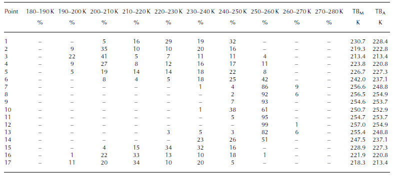
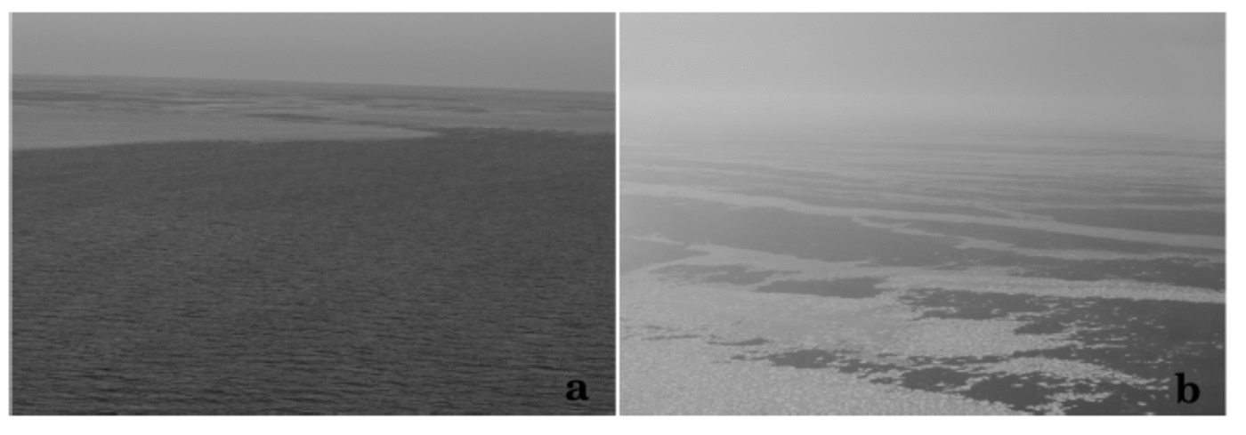
Figure 4 shows the comparison of helicopter-borne 36GHz-H TBs and PR36 with MODIS ice thickness and ice thickness information from a shipborne video camera, along the flight track in Figure 1. Because the MODIS ice thickness algorithm is applicable only to sea ice with thicknesses <0.5 m (Reference Yu and RothrockYu and Rothrock, 1996), MODIS-derived ice thicknesses above 0.5 m are not shown here. The helicopter data were acquired within ± 9 hours of the satellite MODIS overpass. The time lag between the shipborne observation and corresponding satellite MODIS data was ∼9-14 hours. Points 1-53 in Figure 4 correspond to the MODIS gridcells along the track. The helicopter data within each gridcell were averaged without any weighting. The number of helicopter data points in each of these MODIS gridcells varied from about 10 to 30. It is noted that the ship track is not exactly the same track of the helicopter. The helicopter-borne PR36 values have no correlation with MODIS ice thicknesses for the areas shown by the arrows in Figure 4. The aerial photos (Fig. 5) corresponding to the regions indicated by these arrows show the coincident ice conditions (a combination of thin ice and open water). These are MIZ regions where sea-ice drift speed is usually higher than in the close pack ice. A substantial change in sea-ice condition in a MODIS gridcell over the 9 hour interval could account for the observed discrepancies.

Fig. 4 Comparison of helicopter-borne 36GHz-H TBs (white circles) and PR36 (black circles with dashed line) with MODIS ice thickness (cross symbols) and ice thickness information from a shipborne video camera (white triangles), along the flight track in the Sea of Okhotsk (see Fig. 1). The dotted line denotes the turning point of the helicopter flight. The two arrows show the area where we took photos from the helicopter (see Fig. 5).
3.2. Southern Ocean
A comparison of 36GHz-H and -V TBs derived from satellite AMSR-II with those from the helicopter-borne radiometer along the flight track (shown in Fig. 2) is presented in Figure 6. To focus on the polynya and iceberg tongue, only data from the Dalton Polynya and its surrounding area (marked by the red circle in Fig. 2b) are shown. In this case, the helicopter data were acquired within ±1 hour of the satellite AMSR-II overpass. The helicopter data within each AMSR-II gridcell along the track were averaged and plotted in a similar way to the Sea of Okhotsk data (Fig. 6). Circles show averaged helicopter-borne radiometer data for each corresponding AMSR-II gridcell with 1 STD error bars. Around the DIT, the iceberg tongue and thin ice usually coexist in one AMSR-II gridcell. AMSR-II gridcells considered here (Fig. 6) include areas beyond the DIT itself. Due to the much coarser grid resolution of the AMSR-II compared to that of the helicopter-borne radiometer, the satellite sensor cannot adequately resolve this boundary. Thus, there is a large difference between AMSR-II and helicopter-borne TBs, with AMSR-II values sometimes being outside the standard deviation of helicopter-borne values. In the DIT region, the differences between AMSR-II and helicopter-borne radiometer TBs are +31 K and +12 K in 36GHz-H and -V, respectively. In the DIT region, AMSR II gridcells partly cover the DIT and also partly cover the open water adjacent to the DIT, so AMSR-II TBs could be influenced by the open water. On the other hand, in other areas outside the DIT regions, the differences between AMSR-II and helicopter-borne radiometer TBs are -0.21 K and +0.68 K in 36GHz-H and -V, respectively. This bias is considered to be good agreement because this is smaller than the precision of the helicopter-borne radiometer (1 K).

Fig. 6. Comparison of 36GHz-H (a) and -V (b) TBs from AMSR-II (black circles and line) with those from the helicopter-borne sensor (white circles with error bars showing ±1 SD in each AMSR-II gridcell) along the flight track around the DIT in the Southern Ocean (see Fig. 2). The results are shown only for the polynya and its surrounding area circled in red in Figure 2. Judging from visual inspection of the photos from the helicopter, the areas of first-year ice (FY), open water and thin ice (OW&TI), and iceberg tongue (DIT) are indicated at the bottom.
The comparison of helicopter-borne PR36 with helicopter-borne pyrometer- and MODIS-derived surface temperature data along the flight track is shown in Figure 7. The helicopter data were acquired within ± 1 hour of the satellite MODIS overpass. In Figure 7, the helicopter data within each MODIS gridcell were averaged in a similar way to the Sea of Okhotsk case. Average values of helicopter-borne radiometer and TIR data (thick line and circles, respectively) are shown for each corresponding MODIS gridcell, with STD error bars for the TIR data. Starting the mowing-the-lawn pattern in the northwest corner, the helicopter observed (in order): first-year ice, thin ice, open water, DIT, open water, thin ice, first-year ice, thin ice, open water, DIT, open water, thin ice and first-year ice. The mean values and their deviations from the helicopter-borne PR values and surface temperature values for these areas are consistent with those shown in past studies (e.g. Reference Scambos, Haran and MassomScambos and others, 2006; Reference Hwang, Ehn and BarberHwang and others, 2008). Conversely, the MODIS results differ from the helicopter-borne TIR results in the thin-ice and open-water areas. Judging from visual inspection of coincident airborne photography from the helicopter, the open-water area mainly comprised a mix of thin ice and open water close to the DIT. The helicopter-borne IR data show surface temperatures in open water that are a little higher than those in thin-ice regions; however, the difference is <0.5 K. MODIS TIR indicates an opposite pattern, with higher surface temperatures over thin ice compared to open water. The reason for this difference is not clear. It might be caused by atmospheric contamination (e.g. ice fogs in polynyas), but the helicopter-borne aerial imagery gave no indication of ice fog for the region concerned. The difference between pyrometer and MODIS in the open-water, thin sea-ice, first-year-ice and DIT regions is +0.14 K, –0.90 K, +0.12 K and +0.23K, respectively (see next paragraph for this categorization). Ultimately, this difference is within the variation of a past MODIS validation experiment (Reference Scambos, Haran and MassomScambos and others, 2006) in the thin-ice region.

Fig. 7. Comparison of the helicopter-borne PR36 (thick line) with the helicopter-borne thermal IR pyrometer (white circles with error bars showing ± 1 SD in each MODIS gridcell) and MODIS-derived surface temperature (thin line) along the same track as in Figure 6 around the DIT. The areas of first-year ice (FY), thin ice (TI), open water (OW) and iceberg tongue (DIT) are indicated at the bottom. The dashed line denotes the freezing point (271.29 K).
Based on coincident helicopter aerial photography, the flight data are categorized into four regions: open water, thin sea ice, first-year ice and DIT. Table 3 provides the mean values of helicopter-borne surface temperatures and PR36 with their standard deviations, for the three different regions. The surface temperature data in the open-water category are nearly equal to those in the thin-ice category (see Fig. 7). However, the difference between the respective PR36 values is large, suggesting that the above categorization by visual inspection is correct. Furthermore, these values agree with previous results from in situ observation and theoretical modeling studies (Reference Hwang, Ehn and BarberHwang and others, 2008). The PR36 value is considered to be ∼0.137 for the thin-ice region in this season. This value also agrees with the previous thin-ice-thickness algorithm using AMSR-E data in the Sea of Okhotsk (Reference Nihashi, Ohshima, Tamura, Fukamachi and SaitohNihashi and others, 2009), showing a PR36 value of 0.12-0.154 for 0.0-0.1 m thin ice.
Table 3. Mean values of surface temperature and PR36 with their standard deviations, for the helicopter-borne survey over the Dalton Polynya (see Fig. 7). Sample numbers of the surface temperature and PR36 (in parentheses) are also shown. Based on coincident helicopter-borne photography, the flight data are categorized into four regions: open water, thin sea ice, first-year ice and DIT

Figure 8a shows the scatter plot of helicopter-borne 36GHz-H and -V TBs. The signals for the sea-ice region and for the DIT form distinctive clusters, suggesting that it is possible to use 36 GHz data to detect regions of iceberg tongue. This is supported by data of the DIT region from the satellite AMSR-II sensor (red crosses in Fig. 8a). We only choose the case where AMSR-II data gridcells are completely inside the DIT. For the difference between the wide range of triangles and the narrow range of red crosses, we speculate that this could relate to location difference inside the DIT and footprint difference. Figure 8b shows the same scatter plot as Figure 8a, but for 36GHz-H TBs and PR36. The solid regression line is for open water, thin ice and first-year ice (black circles). These sea-ice data correlate well, while the DIT data (triangles) follow a different regression (not shown). Therefore, this characteristic can be used for the detection of iceberg tongue conditions. The 36 GHz TBs from AMSR-E and AMSR-II may support the detection of confluence regions of icebergs, so-called iceberg tongues, judging from the extent of the distance from the regression line of Figure 8b. Although additional analysis will be required, confirmation of the above characteristics could be a basis for improving satellite PMW algorithms.

Fig. 8. (a) Comparison of helicopter-borne 36GHz-H TBs and 36GHz-V TBs during Dalton Polynya survey. Black circles show data for the sea-ice region including open water, thin ice and first-year ice. Triangles show data of the DIT. Red crosses show data of the DIT from the satellite AMSR-II sensor. The two solid lines show PR36 values of 0.02 and 0.12. (b) Same comparison as (a) for 36GHz-H TBs and PR36. The solid line shows the regression line for black circles. The equation and correlation coefficient of the regression line are also shown.
4. Concluding Remarks
This study presents the results from two airborne surveys to aid evaluation of satellite PMW estimates of thin sea-ice distribution in coastal polynyas and the MIZ of both hemispheres. We used a helicopter-borne portable PMW radiometer operating at a frequency of 36 GHz (similar to one channel of the spaceborne AMSR-E and AMSR-II) in the sea-ice region (including thin-ice area) of the Sea of Okhotsk and the Southern Ocean. Our operation is the first helicopter-borne PMW observation in this region. The aim of these helicopter-borne observations is to connect large-scale satellite and highly detailed in situ observations (e.g. shipborne observation), whose footprints are significantly different. Except for the coastal zone where sea-ice conditions cannot be resolved by the satellite sensors (e.g. around the DIT), AMSR-E and AMSR-II TBs are close to the mean values of the helicopter-borne radiometer’s TBs. In the marginal ice zone and first-year sea-ice region of the Sea of Okhotsk with non-uniform ice thickness, the AMSR-E TBs are closer to the mean values of the helicopter-borne TBs, compared to the mode of the helicopter-borne TBs. In the Sea of Okhotsk experiment, the helicopter-borne PR36 values tend to increase as MODIS ice thickness decreases.
In the Southern Ocean experiment, airborne data were collected over first-year ice, thin ice, open water and iceberg tongue. The mean values and their deviations from the helicopter-borne PR36 and surface temperature values, subject to the sea-ice conditions, are consistent with those found in past studies. Based on visual inspection of helicopter aerial photography, the flight data were categorized into four regions: open water, thin sea-ice, first-year sea ice and DIT. The PR36 for thin ice of the Dalton Polynya with quite uniform surface temperature, and hence presumably ice thickness, is estimated to be 0.137 in October. This value agrees with previous in situ observations and theoretical modeling (Reference Hwang, Ehn and BarberHwang and others, 2008), and again agrees with the AMSR-E thin-ice thickness algorithm for the Sea of Okhotsk of Reference Nihashi, Ohshima, Tamura, Fukamachi and SaitohNihashi and others (2009). Over the DIT, the helicopter-borne 36 GHz TBs are substantially different from those of the other surface types encountered, suggesting that a combination of vertically and horizontally polarized 36 GHz TBs can be used to distinguish ice typical of an Antarctic iceberg tongue from other surface types.
Airborne measurements are well suited to bridging the gap between highly detailed but very localized in situ observations and large-scale satellite data. The results presented here make a useful contribution to validating thin sea-ice thickness algorithms applied to spaceborne data. For improvement of the measurement strategy with the helicopter, morning flight and the time-synchronized operation with satellite observation are both important. Further experiments are required to extend the airborne capability, possibly from fixed-wing aircraft.
Acknowledgements
We sincerely acknowledge K. Meiners, S. Whiteside, pilots and engineers of Helicopter Resources Pty Ltd, and the masters and crew of RV Aurora Australis and P/V Soya. We also acknowledge two anonymous reviewers, Scientific Editor S. Kern and Chief Editor P. Heil for instructive comments and useful information. The AMSR-E data were provided by NSIDC, University of Colorado, and the AMSR-II data by JAXA. The MODIS data were obtained from the NASA level 1 Atmosphere Archive and Distribution System (http://ladsweb.nascom.nasa.gov/). The ERA-Interim data were obtained from ECMWF (http://data.ecmwf.int/data/) . This work was supported by the Core Research for Evolutional Science and Technology, from the Grants-in-Aid for Scientific Research (20221001, 24810030, 2503748, 25241001 and 26740007), from the Center for the Promotion of Integrated Sciences of Sokendai, from the Canon Foundation and from JAXA’s Global Change Observation Mission 1st-Water (GCOM-W1). This study was supported partly by the Grant for Joint Research Program of the Institute of Low Temperature Science, Hokkaido University. Southern Ocean data were collected under Australian Antarctic Science Project 4073, supported by the Australian Government’s Cooperative Research Centers Program through the Antarctic Climate & Ecosystems Cooperative Research Center.
Author Contribution Statement
T.Ta. led this study. T.Ta. and K.I.O. conducted this project after planning the experiment with J.L.L., T.To., R.A.M. and S.U. T.Ta. led the analysis with J.L.L., T.To., D.N. and A.D.F., and the fieldwork with J.L.L., K.T., K.Na., P.W.J. and K.B.Ne. All authors discussed the results and commented on the manuscript.


