


Impact Statement
This work demonstrates how SerpentFlow, a generative AI-based domain alignment method, can perform statistical downscaling of wind variables from coarse-resolution climate simulations without paired observations. It produces spatially coherent, multivariate-consistent fine-scale wind fields while simultaneously correcting biases and improving the representation of extremes and intervariable dependencies. As a low-cost alternative to dynamical downscaling, SerpentFlow facilitates the generation of local-scale climate data, supporting wind-related climate impact studies.
1. Introduction
Anthropogenic climate change entails changes in atmospheric circulation and the statistical properties of climate variables, with important consequences for natural and socio-economic systems. General circulation models (GCMs) are the primary tools used to simulate these changes and produce climate projections under different emission scenarios. While GCMs provide a physically consistent representation of the climate system at the global scale, their coarse spatial resolution and systematic biases limit their direct use for regional and local impact studies (Maraun et al., Reference Maraun, Wetterhall, Ireson, Chandler, Kendon, Widmann, Brienen, Rust, Sauter, Themeßl, Venema, Chun, Goodess, Jones, Onof, Vrac and Thiele-Eich2010; Teutschbein and Seibert, Reference Teutschbein and Seibert2012).
Many climate impact applications require climate information that is spatially coherent, multivariate, and physically plausible at fine spatial scales. This is particularly important for wind-related applications, such as wind energy assessments, which depend on the joint behavior of wind speed, direction, variability, and extremes. GCM outputs are therefore commonly post-processed using downscaling and bias correction methods (Bartók et al., Reference Bartók, Tobin, Vautard, Vrac, Jin, Levavasseur, Denvil, Dubus, Parey, Michelangeli, Troccoli and Saint-Drenan2019).
Statistical downscaling and bias correction provide a computationally efficient alternative to dynamical downscaling by learning empirical relationships between climate simulations and observations. Classical approaches include distribution-based methods such as CDF-t (Michelangeli et al., Reference Michelangeli, Vrac and Loukos2009; Vrac and Friederichs, Reference Vrac and Friederichs2015) and multivariate frameworks such as MBCn (Cannon, Reference Cannon2018), DOTC (Robin et al., Reference Robin, Vrac, Naveau and Yiou2019), R2D2 (Vrac and Thao, Reference Vrac and Thao2020), and MRec (Zhang, Reference Zhang2021). While multivariate methods better preserve intervariable dependencies, challenges remain for high-dimensional, spatially structured fields, particularly in maintaining spatial coherence under nonstationary climate conditions (François et al., Reference François, Vrac, Cannon, Robin and Allard2020; Allard et al., Reference Allard, Vrac, François and García de Cortázar-Atauri2025).
Machine learning approaches, especially deep learning, have been increasingly explored for downscaling and bias correction. These models can capture complex nonlinear relationships and spatial structures, showing promising results across climate variables (Vandal et al., Reference Vandal, Kodra, Ganguly, Michaelis, Nemani and Ganguly2017; Soares et al., Reference Soares, Johannsen, Lima, Lemos, Bento and Bushenkova2024). Most approaches rely on supervised learning with paired low- and high-resolution datasets, which are rarely available in realistic climate projection settings, making explicit pairing ill-defined (Bartók et al., Reference Bartók, Tobin, Vautard, Vrac, Jin, Levavasseur, Denvil, Dubus, Parey, Michelangeli, Troccoli and Saint-Drenan2019). Consequently, many studies adopt perfect-model or synthetic training frameworks that do not fully reflect real-world applications.
These limitations have motivated interest in generative and probabilistic approaches that operate in unpaired or weakly supervised settings. Generative domain adaptation methods align climate model outputs and observations within a common distribution while preserving spatial structure and providing a measure of uncertainty. Recent studies explore adversarial learning (Groenke et al., Reference Groenke, Madaus and Monteleoni2020), diffusion bridge-based models (Bischoff and Deck, Reference Bischoff and Deck2024; Hess et al., Reference Hess, Aich, Pan and Boers2025), and hybrid approaches combining optimal transport and generative sampling (Wan et al., Reference Wan, Baptista, Chen, Anderson, Boral, Sha and Zepeda-Núñez2023). While promising, these methods rely on implicit alignment mechanisms—cycle-consistency losses, Gaussian latent spaces, or diffusion paths—to bridge the gap between domains, without explicitly defining what should be shared and what should differ. As we show in the results, and as also reported in Keisler et al. (Reference Keisler, Charantonis, Goude, Oueslati and Monteleoni2026), some of these approaches fail to preserve the large-scale dynamics of the driving GCM: the downscaled fields can drift away from the source signal even at scales that the GCM resolves well, making it difficult to trust their projections under future climate conditions. This lack of an interpretable, physically grounded separation of scales calls for methods that explicitly control which information is retained from the source and which is generated.
Frequency-based decompositions offer a natural framework for this purpose. Gaussian filtering and Fourier cutoffs have a long history in fluid dynamics, from subgrid-scale modeling in Large Eddy Simulations to more recent super-resolution and data reconstruction approaches for turbulent flows (Buzzicotti, Reference Buzzicotti2023; Suresh Babu et al., Reference Suresh Babu, Sadam and Lermusiaux2026). These methods explicitly separate resolved and unresolved scales, providing both physical interpretability and control over the scale-dependent behavior of the reconstruction.
In this work, we investigate SerpentFlow (Keisler et al., Reference Keisler, Charantonis, Goude, Oueslati and Monteleoni2026), an interpretable generative domain adaptation framework for multivariate downscaling and bias correction. SerpentFlow operates in an unpaired setting by constructing pseudo low−/high-resolution pairs through an explicit separation of spatial scales: large-scale patterns are aligned between climate model outputs and observations, while small-scale variability is learned conditionally via a flow-matching generative model. This enables generation of fine-scale wind variability while maintaining physically meaningful large-scale climate information.
We apply SerpentFlow to multiple near-surface wind variables, including wind speed, zonal and meridional components, and maximum wind speed, evaluating its performance in both historical and future climate conditions. Comparisons with established multivariate bias correction methods focus on spatial coherence, intervariable consistency, and robustness under climate change, highlighting the potential of interpretable generative domain adaptation for wind energy impact studies (The code is available here: https://github.com/JulieKeisler/serpentflow).
The main contributions of this work are:
-
• Application of an interpretable generative domain adaptation framework, SerpentFlow, for multivariate downscaling and bias correction of wind variables in an unpaired setting.
-
• Introduction of a Gaussian-blur-based decomposition to handle irregular observational domains, enabling flexible separation of large-scale and local features even when Fourier-based filtering is not applicable.
-
• Comprehensive evaluation against established downscaling and bias correction methods, assessing distributions, spatial structure, intervariable relationships, and robustness under future climate.
2. Method
Our work uses SerpentFlow (Keisler et al., Reference Keisler, Charantonis, Goude, Oueslati and Monteleoni2026), a generative domain adaptation framework designed for unpaired multivariate downscaling and bias correction. While we do not modify the original method, we provide a brief overview to clarify its main principles and how it applies to wind variables.
2.1. Core idea
SerpentFlow transfers samples from a source domain (coarse GCM outputs) to a target domain (observations or reanalyses) by representing each field in a latent space and separating it into a shared and domain-specific component. The shared component captures structures common to both domains, while the domain-specific component encodes elements unique to each domain. During training, pseudo-pairs are constructed by combining the shared component of a target sample with stochastic realizations of its domain-specific part. A generative model then learns to reconstruct the target field conditioned on the shared component. At inference, source samples are projected into the shared-domain space, combined with stochastic noise in the domain-specific component, and mapped to the target domain through the learned generative model.
2.2. Frequency-based latent space
In practice, SerpentFlow implements the shared-domain hypothesis in the Fourier domain for unsupervised super-resolution. Fields are decomposed into spatial frequencies, with low-frequency modes representing large-scale shared structures and high-frequency modes representing domain-specific variability. This decomposition is conceptually analogous to the Reynolds decomposition used in atmospheric science (Reynolds, Reference Reynolds1895), which separates a flow into its mean and fluctuating components—here, the cutoff frequency
$ {\omega}_{cut} $
 plays the role of the scale separator between resolved large-scale dynamics and unresolved fine-scale variability. As stated in Keisler et al. (Reference Keisler, Charantonis, Goude, Oueslati and Monteleoni2026), the cutoff can be determined automatically by a classifier trained to distinguish between domains, providing a convenient strategy for hyperparameter tuning. Alternatively, for climate downscaling, a more interpretable choice consists in setting
$ {\omega}_{cut} $
plays the role of the scale separator between resolved large-scale dynamics and unresolved fine-scale variability. As stated in Keisler et al. (Reference Keisler, Charantonis, Goude, Oueslati and Monteleoni2026), the cutoff can be determined automatically by a classifier trained to distinguish between domains, providing a convenient strategy for hyperparameter tuning. Alternatively, for climate downscaling, a more interpretable choice consists in setting
$ {\omega}_{cut} $
 to match the effective resolution of the driving GCM (Abdalla, Reference Abdalla2013), directly linking the scale separation to the physical resolution gap between models. As we confirm in the results, the cutoff identified by the classifier indeed corresponds to the effective resolution of the GCM, bridging both approaches. This frequency-based latent space provides an interpretable and physically meaningful separation of scales, naturally suited for super-resolution tasks such as wind downscaling.
2.3. Generative mapping
SerpentFlow is agnostic to the choice of the generative model
$ {f}_{\theta } $
 . In the original implementation, flow matching (Lipman et al., Reference Lipman, Chen, Ben-Hamu, Nickel and Le2023) is used to learn a continuous mapping from pseudo-inputs to target fields. This allows the model to generate physically plausible fine-scale details while respecting the shared large-scale patterns. In inference, coarse GCM wind fields are projected into the shared-frequency space, and the learned generator produces downscaled and bias-corrected wind variables consistent with the target distribution.
2.4. Practical workflow
Figure 1 illustrates the training and inference workflow. Pseudo-pairs generated from high-resolution observations/reanalyses are used to train
$ {f}_{\theta } $
 , and coarse GCM fields are subsequently downscaled through the same pipeline. The resulting outputs are physically coherent, statistically consistent, and preserve both large-scale climate dynamics and realistic small-scale variations.
Overview of the training and inference pipeline of SerpentFlow, a generative domain-adaptation method for statistical downscaling via shared-structure.
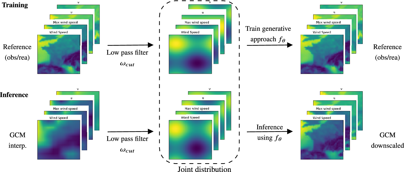
Figure 1. Long description
The flowchart is divided into two horizontal rows: Training at the top and Inference at the bottom.
In the Training row, the process begins on the left with Reference (obs/rea) data, shown as a stack of four heatmaps labeled Wind Speed, Max wind speed, u, and v. An arrow labeled Low pass filter omega sub cut points to a central dashed box. Inside this box, the heatmaps appear blurred, labeled as Joint distribution. An arrow labeled Train generative approach f sub theta points to the final output on the right, which restores the original high-resolution Reference (obs/rea) heatmaps.
In the Inference row, the process begins on the left with G C M interp. data, shown as a similar stack of four heatmaps. An arrow labeled Low pass filter omega sub cut points to the same central Joint distribution box. From this central box, an arrow labeled Inference using f sub theta points to the final output on the right, labeled G C M downscaled. This output shows high-resolution heatmaps reconstructed from the interpolated input data.
(1) Decompose target fields into low/high frequencies and generate pseudo-pairs, (2) train the generative model to reconstruct high-resolution fields conditioned on low-frequency structure, and (3) project source fields into the shared space and apply the trained generator to obtain downscaled and bias-corrected outputs.
For full technical details and theoretical background, we refer the reader to Keisler et al. (Reference Keisler, Charantonis, Goude, Oueslati and Monteleoni2026).
3. Experiments
3.1. Data and study domain
We evaluate SerpentFlow and baseline methods over the French territory using outputs from the ACCESS Earth System Model (Ziehn et al., Reference Ziehn, Chamberlain, Law, Lenton, Bodman, Dix, Stevens, Wang and Srbinovsky2020) (
$ {1.9}^{\circ}\times {1.2}^{\circ } $
 , 145 km
$ \times $
, 145 km
$ \times $
 130 km) under the SSP2-4.5 scenario. ACCESS is a participating model in the Coupled Model Intercomparison Project Phase 6 (O’Neill et al., Reference O’Neill, Tebaldi, van Vuuren, Eyring, Friedlingstein, Hurtt, Knutti, Kriegler, Lamarque, Lowe, Meehl, Moss, Riahi and Sanderson2016), an international framework designed to coordinate and standardize climate model experiments. Our analysis focuses on four near-surface wind variables: wind speed (sfcWind), maximum wind speed (sfcWindMax), and the zonal (uas) and meridional (vas) components. ERA5 (Hersbach et al., Reference Hersbach, Bell, Berrisford, Hirahara, Horányi, Muñoz-Sabater, Nicolas, Peubey, Radu, Schepers, Simmons, Soci, Abdalla, Abellan, Balsamo, Bechtold, Biavati, Bidlot, Bonavita, de Chiara, Dahlgren, Dee, Diamantakis, Dragani, Flemming, Forbes, Fuentes, Geer, Haimberger, Healy, Hogan, Hólm, Janisková, Keeley, Laloyaux, Lopez, Lupu, Radnoti, de Rosnay, Rozum, Vamborg, Villaume and Thépaut2020,
$ {0.25}^{\circ}\times {0.25}^{\circ } $
130 km) under the SSP2-4.5 scenario. ACCESS is a participating model in the Coupled Model Intercomparison Project Phase 6 (O’Neill et al., Reference O’Neill, Tebaldi, van Vuuren, Eyring, Friedlingstein, Hurtt, Knutti, Kriegler, Lamarque, Lowe, Meehl, Moss, Riahi and Sanderson2016), an international framework designed to coordinate and standardize climate model experiments. Our analysis focuses on four near-surface wind variables: wind speed (sfcWind), maximum wind speed (sfcWindMax), and the zonal (uas) and meridional (vas) components. ERA5 (Hersbach et al., Reference Hersbach, Bell, Berrisford, Hirahara, Horányi, Muñoz-Sabater, Nicolas, Peubey, Radu, Schepers, Simmons, Soci, Abdalla, Abellan, Balsamo, Bechtold, Biavati, Bidlot, Bonavita, de Chiara, Dahlgren, Dee, Diamantakis, Dragani, Flemming, Forbes, Fuentes, Geer, Haimberger, Healy, Hogan, Hólm, Janisková, Keeley, Laloyaux, Lopez, Lupu, Radnoti, de Rosnay, Rozum, Vamborg, Villaume and Thépaut2020,
$ {0.25}^{\circ}\times {0.25}^{\circ } $
 , 25 km) reanalyses, averaged at a daily temporal resolution, serve as the observational reference.
The dataset is split to maximize training data while keeping independent evaluation periods. All GCM fields are bilinearly interpolated to the ERA5 grid prior to computing metrics and producing plots.
-
• Training (1979–1999): used to learn the statistical mapping between GCM outputs and ERA5 observations.
-
• Evaluation against ERA5 (2000–2020): assesses historical bias correction and downscaling performance.
-
• Evaluation against GCM projections (2000–2100): assesses the consistency of downscaling methods under future climate conditions. This evaluation is necessary because some statistical downscaling methods can alter the large-scale dynamics of the driving GCM, introducing spurious trends or distorting the climate change signal. By comparing downscaled outputs against the raw GCM projections, we verify that the downscaling preserves the broad physical consistency of the climate system over the full projection period.
GCM outputs are regridded to the ERA5 resolution before downscaling: linear interpolation is used for baseline methods, while SerpentFlow employs a spectral interpolation as described by Keisler et al. (Reference Keisler, Charantonis, Goude, Oueslati and Monteleoni2026).
3.2. Baselines
We compare the following approaches:
-
• CDF-t (Michelangeli et al., Reference Michelangeli, Vrac and Loukos2009; Vrac and Friederichs, Reference Vrac and Friederichs2015): a univariate bias correction method that maps quantiles between distributions, implemented as in François et al. (Reference François, Vrac, Cannon, Robin and Allard2020). Unlike simpler quantile mapping approaches, CDF-t explicitly accounts for the evolution of the GCM distribution between the historical and future periods, allowing it to preserve the climate change signal during correction. Moreover, wind variables—unlike temperature—do not exhibit a strong systematic shift in their overall distribution under future climate scenarios, which further limits the risk of degraded performance over the projection period.
-
• R2D2 (Vrac and Thao, Reference Vrac and Thao2020): a multivariate stochastic bias correction method that preserves intervariable dependencies. Due to computational constraints, we process the domain using $ 5\times 5 $
 pixel patches.
 -
• Dual FM: a domain adaptation method implemented in Keisler et al. (Reference Keisler, Charantonis, Goude, Oueslati and Monteleoni2026), inspired by ClimAlign (Groenke et al., Reference Groenke, Madaus and Monteleoni2020), but replacing normalizing flows with flow matching.
-
• SerpentFlow (Keisler et al., Reference Keisler, Charantonis, Goude, Oueslati and Monteleoni2026): the full method, sharing the UNet generator architecture with Dual FM. SerpentFlow decomposes fields into three Fourier-based frequency bands (cutoff scales: 1200, 750, 300 km) to separate large-scale shared structures from finer domain-specific patterns, enabling control over scale-dependent downscaling performance. The primary cutoff frequency of 1200 km was identified by the classifier described in Keisler et al. (Reference Keisler, Charantonis, Goude, Oueslati and Monteleoni2026), and also corresponds to the effective resolution of the GCM (Abdalla, Reference Abdalla2013). To explore the sensitivity to this cutoff, we additionally tested two lower values (750 and 300 km), which allow more fine-scale information from the GCM to pass into the shared representation.

For deep learning-based methods (SerpentFlow and Dual FM), we generate 10 ensemble members per simulation. We report both the ensemble mean and the output of a single member (for SerpentFlow at 1200 km cutoff), the latter corresponding to the baseline in Keisler et al. (Reference Keisler, Charantonis, Goude, Oueslati and Monteleoni2026). While Dual FM has been described as a generative model, our analysis shows that its integration of an ODE makes the outputs effectively deterministic, so the ensemble mean and a single member are identical (discussed Supplementary Figure S26). Inputs are normalized using the spatial mean and standard deviation of the training period (GCM statistics for source fields, ERA5 statistics for target fields), and outputs are denormalized using ERA5 mean and standard deviation at each grid point.
3.3. Results
We evaluate the downscaling and bias correction methods from two complementary perspectives. First, we assess their ability to reproduce the statistical and spatial characteristics of the observational reference (ERA5), which is critical for impact and energy applications. Second, we examine whether the methods preserve the large-scale climate dynamics and temporal evolution of the original GCM projections, a key requirement for climate change studies. Regarding computational cost, training SerpentFlow for a given cutoff frequency
$ {\omega}_{cut} $
 requires approximately 4 hours on a single NVIDIA H100 GPU using 20 years of training data. Once trained, generating a single ensemble member over a 100-year projection takes roughly 10 minutes. Dual FM, which requires training two separate Flow Matching models (one per domain), approximately doubles both training and inference time. Importantly, the GCM only intervenes in the SerpentFlow training pipeline through the choice of
$ {\omega}_{cut} $
requires approximately 4 hours on a single NVIDIA H100 GPU using 20 years of training data. Once trained, generating a single ensemble member over a 100-year projection takes roughly 10 minutes. Dual FM, which requires training two separate Flow Matching models (one per domain), approximately doubles both training and inference time. Importantly, the GCM only intervenes in the SerpentFlow training pipeline through the choice of
$ {\omega}_{cut} $
 : the generator
$ {f}_{\theta } $
: the generator
$ {f}_{\theta } $
 is trained exclusively on the target domain. This means that a trained model can be directly applied to any GCM sharing the same effective resolution, without retraining—substantially reducing the computational burden when downscaling multi-model ensembles.
Evaluation metrics and protocols are provided in Supplementary Appendix A, while detailed spatial maps, distributional diagnostics, and time series are available in Supplementary Appendix C.
Overview
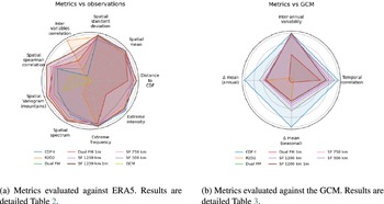
Figure 2 summarizes the performance of all methods using radar plots, where each axis represents a different metric and values closer to the outer edge indicate better performance. The left panel shows comparison against ERA5, highlighting the methods’ ability to reproduce observational statistics, whereas the right panel evaluates consistency with the raw GCM projections, emphasizing preservation of large-scale dynamics.
Radar plots summarizing the performance of all methods averaged over all climate variables (results on average wind speed only are given Supplementary Figure S7). Higher values (closer to the outer circle) indicate better agreement with the reference. SF stands for SerpentFlow in all the plots, and “mbr” indicates “one member” for a generative method, the average of the members being shown otherwise.
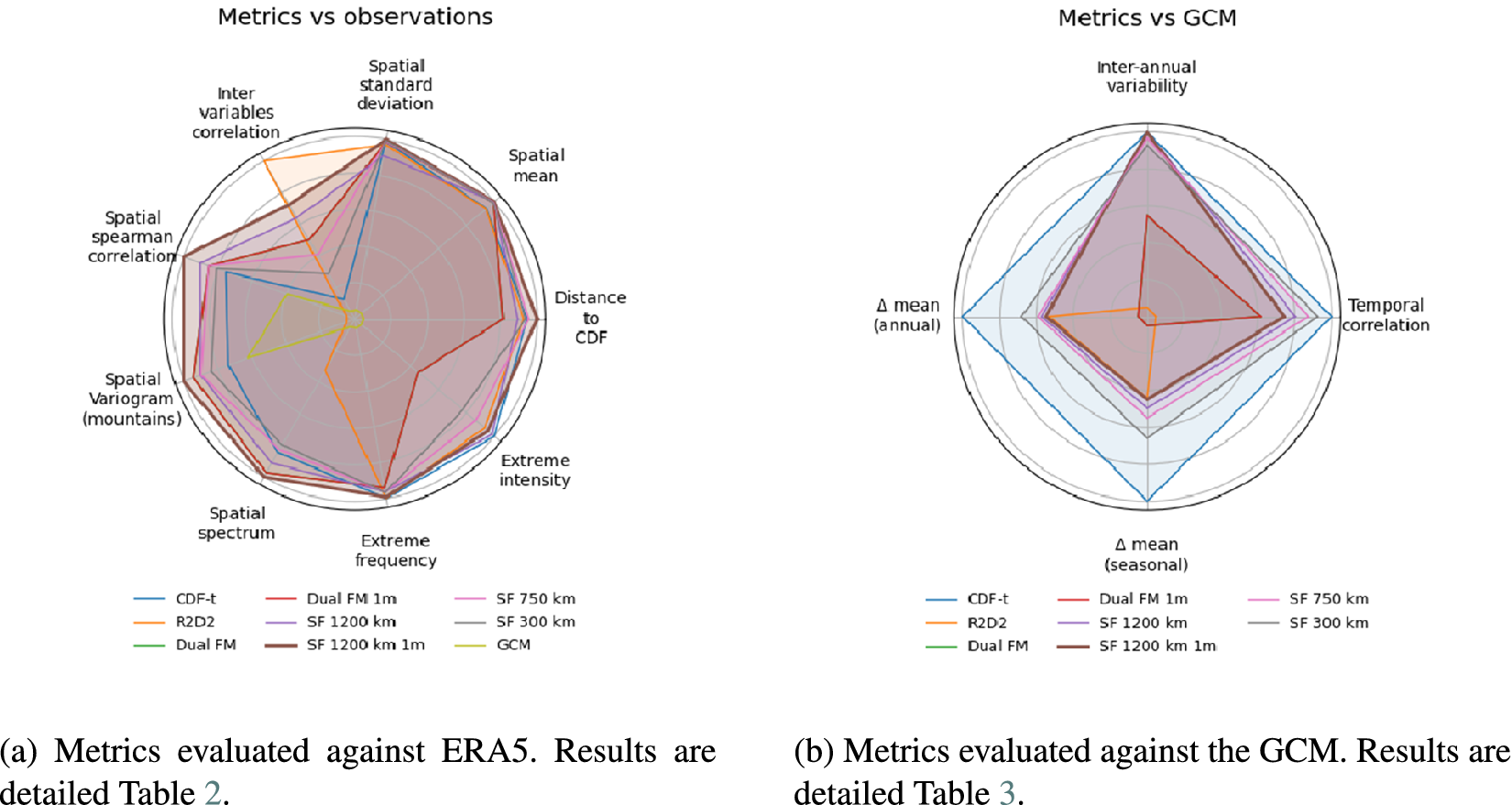
Figure 2. Long description
The figure consists of two panels, a and b.
Panel a, titled Metrics vs observations, features a radar chart with nine axes arranged clockwise: Spatial standard deviation, Spatial mean, Distance to C D F, Extreme intensity, Extreme frequency, Spatial spectrum, Spatial Variogram (mountains), Spatial spearman correlation, and Inter variables correlation. Most methods, including C D F-t, Dual F M, and various S F (SerpentFlow) configurations, show high performance, with their polygons extending near the outer perimeter across most metrics. The R 2 D 2 and G C M methods show significantly lower agreement, with their polygons collapsed toward the center, particularly in spatial correlations and variograms.
Panel b, titled Metrics vs G C M, features a radar chart with four axes: Inter-annual variability, Temporal correlation, Delta mean (seasonal), and Delta mean (annual). The C D F-t method (blue) shows the widest coverage, reaching the outer circle for temporal correlation and seasonal delta mean. The S F methods (shades of purple and brown) form a tight, consistent cluster reaching approximately 75 percent of the way to the perimeter. The R 2 D 2 method (orange) shows the lowest performance, remaining closest to the center across all four axes.
A shared legend at the bottom identifies the methods: C D F-t (blue), R 2 D 2 (orange), Dual F M (green), Dual F M 1 m (red), S F 1200 km (purple), S F 1200 km 1 m (brown), S F 750 km (pink), S F 300 km (gray), and G C M (yellow-green).
Evaluation against ERA5
The left panel of Figure 2a highlights clear differences between classical statistical methods and deep learning based approaches. CDF-t performs well for distributional similarity (Supplementary Figures S10–S12) and extreme-event metrics, but its performance is weaker for intervariable relationships (Supplementary Figures S13–S16) and spatial correlations (Supplementary Figures S17 and S19), especially in mountainous regions (Supplementary Figure S20), reflecting its univariate nature.
R2D2 improves intervariable dependencies compared to CDF-t, but remains limited in reproducing spatial coherence and extremes (Supplementary Figures S13–S16).
Deep learning methods consistently outperform the statistical baselines in reconstructing ERA5’s spatial dynamics (Supplementary Figure S17). While Dual FM improves the spatial spectrum (Supplementary Figure S19), it struggles to capture extreme-value distributions and is less effective than certain SerpentFlow configurations across most metrics. Thanks to its generative nature, SerpentFlow can represent a range of possible values at a given grid point and time (see Supplementary Figure S26), effectively capturing uncertainty in the reconstructed fields. A calibration study for SF 1200 km is given section B. The cutoff scale strongly influences performance: smaller cutoffs (e.g., 300 km) better preserve large-scale coherence but may reduce spatial consistency (Supplementary Figures S18 and S19), whereas larger cutoffs (e.g., 1200 km), especially the one-member version (SF 1200 kmmbr), achieves high values across all ERA5 metrics. Overall, SF 1200 kmmbr provides the best balance between distributional accuracy, spatial coherence, and intervariable consistency.
Consistency with GCM projections
The right panel of Figure 2b evaluates how well the downscaled outputs preserve the large-scale temporal dynamics of the GCM. As expected, CDF-t closely follows the GCM for mean changes and temporal correlations (Supplementary Figures S22–S25). R2D2 performs worse for temporal metrics, reflecting partial loss of large-scale climate signals, partly due to the
$ 5\times 5 $
 patching, which reduces spatial coherence (Supplementary Figure S22).
Dual FM struggles to follow the GCM signal and is consistently outperformed by SerpentFlow across all metrics, performing worst on the delta metrics (Supplementary Figures S23–S25). SerpentFlow, while slightly below CDF-t, better preserves interannual variability and temporal correlations than R2D2 and Dual FM. The performance trade-off is controlled by the cutoff frequency: higher cutoffs retain more GCM dynamics but reduce similarity to observations, whereas lower cutoffs improve agreement with observations at the cost of some large-scale consistency. This allows users to select an appropriate balance depending on the application.
Taken together, these results demonstrate that SerpentFlow provides a favorable trade-off, substantially improving agreement with observations while preserving the essential large-scale dynamics of the driving GCM.
3.4. Univariate application
To further illustrate SerpentFlow’s flexibility, we applied it to a univariate downscaling task for near-surface wind speed, using outputs from the CNRM-CM6-1 climate model (Voldoire et al., Reference Voldoire, Saint-Martin, Sénési, Decharme, Alias, Chevallier, Colin, Guérémy, Michou, Moine, Nabat, Roehrig, Salas y Mélia, Séférian, Valcke, Beau, Belamari, Berthet, Cassou, Cattiaux, Deshayes, Douville, Ethé, Franchistéguy, Geoffroy, Lévy, Madec, Meurdesoif, Msadek, Ribes, Sanchez-Gomez, Terray and Waldman2019) under the SSP3-7.0 scenario (
$ {1.4}^{\circ}\times {1.4}^{\circ } $
 ,130 km) and the high-resolution SAFRAN reanalysis (Vidal et al., Reference Vidal, Martin, Franchistéguy, Baillon and Soubeyroux2010, 8 km), at daily temporal resolution. This application serves several purposes. First, it demonstrates that SerpentFlow can operate without relying on a standard Fourier-based low-pass filter. Instead, we introduce a Gaussian-blur-based decomposition to separate a large-scale “shared-domain” component from a domain-specific residual. This approach enables the method to handle irregular domains, such as land-only observations from SAFRAN, where a Fourier decomposition would produce NaNs over the ocean. Second, it shows that SerpentFlow can work with higher-resolution observational data: whereas previous experiments used ERA5 (25 km), this setup leverages SAFRAN at 8 km, illustrating the method’s scalability and adaptability to finer spatial grids. Third, it generalizes the evaluation to a different GCM and scenario, confirming that SerpentFlow is not tied to a single climate model or pathway. Finally, for this particular setup with CNRM-CM6-1 and SAFRAN, we also have a dynamically downscaled reference provided by the CNRM-Aladin regional climate model (RCM; Colin et al., Reference Colin, Déqué, Radu and Somot2010) (12.5 km resolution) corrected using CDF-t. This allows us to compare statistical (SerpentFlow) and dynamical (RCM) downscaling approaches, highlighting their respective limitations and strengths, and illustrating how they could be used complementarily to improve local-scale climate projections. To prepare for the subsequent mathematical description, it is important to emphasize the goal of the Gaussian-blur-based decomposition: it provides a simple, flexible way to separate large-scale patterns from local-scale variability, while respecting irregular observational domains.
Gaussian-blur-based decomposition
Let
$ x $
 denote the input wind-speed field and
$ \sigma $
denote the input wind-speed field and
$ \sigma $
 denote the standard deviation of the Gaussian kernel controlling the blur. The Gaussian-blur-based decomposition separates
$ x $
denote the standard deviation of the Gaussian kernel controlling the blur. The Gaussian-blur-based decomposition separates
$ x $
 into a large-scale shared component
$ \mu =\mathrm{GaussianBlur}\left(x,\sigma \right) $
into a large-scale shared component
$ \mu =\mathrm{GaussianBlur}\left(x,\sigma \right) $
 , ignoring missing values, and a high-frequency residual
$ {\epsilon}_{\mathrm{HF}}=\epsilon -\mathrm{GaussianBlur}\left(\epsilon, \sigma \right) $
, ignoring missing values, and a high-frequency residual
$ {\epsilon}_{\mathrm{HF}}=\epsilon -\mathrm{GaussianBlur}\left(\epsilon, \sigma \right) $
 with stochastic noise
$ \epsilon \sim \mathcal{N}\left(0,\mathbf{I}\right) $
with stochastic noise
$ \epsilon \sim \mathcal{N}\left(0,\mathbf{I}\right) $
 . Pseudo-training pairs for the target domain are then constructed as
$ {\tilde{x}}_B={\mu}_B+{\unicode{x025B}}_{\mathrm{HF}} $
. Pseudo-training pairs for the target domain are then constructed as
$ {\tilde{x}}_B={\mu}_B+{\unicode{x025B}}_{\mathrm{HF}} $
 , where
$ {\mu}_B $
, where
$ {\mu}_B $
 denotes the shared component of the target field. The blur intensity
$ \sigma $
denotes the shared component of the target field. The blur intensity
$ \sigma $
 plays a role analogous to the cutoff frequency
$ {\omega}_{\mathrm{cut}} $
plays a role analogous to the cutoff frequency
$ {\omega}_{\mathrm{cut}} $
 in the Fourier decomposition: larger
$ \sigma $
in the Fourier decomposition: larger
$ \sigma $
 retains only very large-scale structures, while smaller
$ \sigma $
retains only very large-scale structures, while smaller
$ \sigma $
 preserves finer-scale details.
Implementation details
-
• Only wind speed (sfcWind) is considered, making this a univariate application.
-
• The same UNet generator architecture from the main SerpentFlow experiments is used.
-
• Pseudo-pairs are constructed using the Gaussian-blur decomposition, enabling training despite missing oceanic values.
-
• Baselines include SerpentFlow at different cutoffs (300, 500, 600, and 750 km, the latter identified by the classifier as the optimal separation scale and matches the GCM effective resolution), CDF-t as in the main experiments, and the RCM CNRM-Aladin (Colin et al., Reference Colin, Déqué, Radu and Somot2010) (12.5 km resolution), bias-corrected using CDF-t on SAFRAN.
-
• Data are split between the training data (1980–2000), evaluation against SAFRAN (2000–2020) and evaluation against GCM projections (2000–2100).
Results
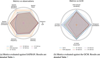
The results (plots in Supplementary Appendix D) are broadly consistent with the ERA5 experiment, confirming the robustness of the findings across datasets, resolutions, GCMs, and scenarios (Figure 3).
Radar plots summarizing the performance of all methods. Higher values (closer to the outer circle) indicate better agreement with the reference.
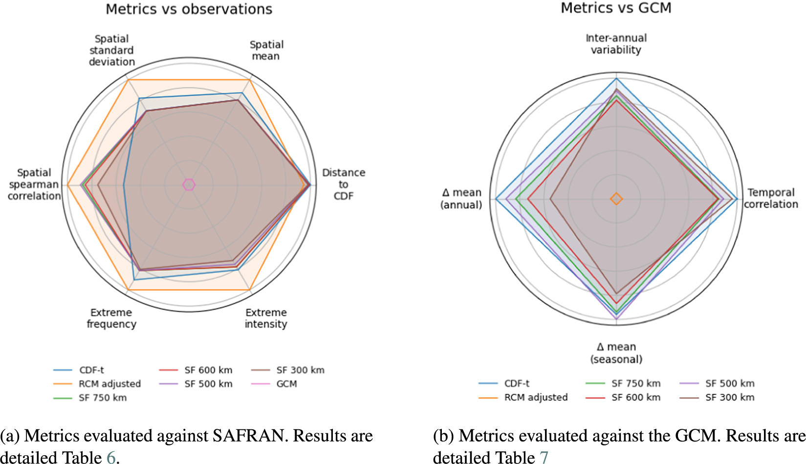
Figure 3. Long description
A two-panel figure showing radar charts for model performance evaluation.
Panel A, titled Metrics vs observations, features a hexagonal radar chart with six axes: Spatial standard deviation at the top, followed clockwise by Spatial mean, Distance to C D F, Extreme intensity, Extreme frequency, and Spatial spearman correlation. The data shows most methods clustered near the outer perimeter, indicating high agreement. The G C M method is the outlier, appearing as a tiny pink hexagon at the very center, indicating poor agreement. The R C M adjusted method, shown in orange, reaches the furthest outer edge on the Spatial standard deviation and Spatial spearman correlation axes.
Panel B, titled Metrics vs G C M, features a diamond-shaped radar chart with four axes: Inter-annual variability at the top, followed clockwise by Temporal correlation, Delta mean (seasonal), and Delta mean (annual). At the center, the R C M adjusted method is represented by a single orange diamond point. The other methods, including C D F-t and various S F scales (750 k m, 600 k m, 500 k m, 300 k m), form concentric diamond shapes. The C D F-t method in blue shows the widest reach on the Inter-annual variability and Delta mean (annual) axes, while the S F 300 k m method in brown is more constrained toward the center.
As expected, the RCM outperforms all statistical baselines on SAFRAN metrics, as it explicitly represents regional-scale processes and boundary conditions inaccessible to statistical methods like SerpentFlow. Its fine-scale dynamics related to topography and surface heterogeneity explain why it does not necessarily follow the temporal evolution of the driving GCM (see Supplementary Figure S34). However, Supplementary Figure S32 shows that SerpentFlow can better capture spatial interactions in some regions, reconstructing physically consistent structures directly from large-scale GCM information without additional dynamical assumptions. This suggests SerpentFlow could be used as a bias-correction method for RCM outputs, rather than relying on CDF-t.
More generally, SerpentFlow substantially outperforms CDF-t in reproducing SAFRAN spatial interactions, while achieving comparable or slightly lower performance on distributional metrics (Supplementary Figure S29), except for extreme local quantiles (Supplementary Figures S30 and S31). The cutoff scale provides control over reconstruction: lower cutoffs yield fields closer to SAFRAN, while higher cutoffs preserve more large-scale GCM characteristics, highlighting a trade-off between local realism and large-scale consistency.
Comparison with the RCM also highlights differences in projected climate change: Supplementary Figures S35 and S36 show that even large-scale future deltas are not preserved by the RCM compared to the driving GCM. Assessing which model provides a more realistic representation of future climate change remains challenging. Local phenomena are not resolved by GCMs, and several studies have shown that some processes and assumptions are not fully represented in RCMs for certain variables (Boé et al., Reference Boé, Somot, Corre and Nabat2020; Nabat et al., Reference Nabat, Somot, Boé, Corre, Katragkou, Li, Mallet, van Meijgaard, Pavlidis, Pietikäinen, Sørland and Solmon2025), including near-surface wind (Wohland, Reference Wohland2022).
Overall, these results emphasize the importance of maintaining diverse downscaling approaches. Dynamical (RCM) and statistical methods, such as SerpentFlow, are complementary and offer different perspectives on regional climate change. In this context, SerpentFlow provides a computationally efficient framework to explore uncertainties and to post-process both GCM and RCM outputs, correcting biases and enhancing spatial resolution.
4. Conclusion
Our evaluation shows that SerpentFlow reproduces ERA5 spatial, temporal, and multivariate characteristics over France while largely preserving large-scale GCM dynamics. Compared to classical statistical methods, it improves spatial coherence, intervariable consistency, and extreme-event representation, and its scale-aware decomposition allows control over the trade-off between local realism and large-scale consistency. Experiments with CNRM-CM6-1 and SAFRAN confirm that these results hold across resolutions, domains, and climate models, including irregular observational grids. Limitations include the short training period and focus on near-surface wind, leaving other variables and longer-term trends for future study. Overall, SerpentFlow demonstrates strong performance as a bias-correction and downscaling method under realistic climate scenarios.
Supplementary material
The supplementary material for this article can be found at http://doi.org/10.1017/eds.2026.10057.
Author contribution
Conceptualization: J.K., B.O., A.C., G.Y., C.M.; Data curation: J.K., B.O.; Data visualization: J.K.; Methodology: J.K., B.O., A.C., Y.G., C.M.; Writing original draft: J.K., B.O., A.C. All authors approved the final submitted draft.
Competing interests
The authors declare none.
Data availability statement
The code is available here: https://github.com/JulieKeisler/serpentflow.
Ethics statement
The research meets all ethical guidelines, including adherence to the legal requirements of the study country.
Funding statement
None.
Provenance statement
This article is part of the Climate Informatics 2026 proceedings and was accepted in Environmental Data Science on the basis of the Climate Informatics peer review process.


 Open access

