





1. Introduction
Chiral active fluids are characterised by a non-vanishing spin-angular momentum density that results in odd contributions to their transport coefficients (Jülicher et al. Reference Jülicher, Grill and Salbreux2018). One example that has attracted significant interest in recent years stems from antisymmetric contributions to the viscosity tensor, called odd viscosity (Avron Reference Avron1998; Banerjee et al. Reference Banerjee, Souslov, Abanov and Vitelli2017; Fruchart, Scheibner & Vitelli Reference Fruchart, Scheibner and Vitelli2023). The effects of odd viscosity on fluid flow have been well documented in recent theoretical work: analytically exact solutions have been obtained for the hydrodynamic flow profiles of two-dimensional rigid disks in compressible fluids with odd viscosity (Daddi-Moussa-Ider, Vilfan & Hosaka Reference Daddi-Moussa-Ider, Vilfan and Hosaka2025), of a spherical particle in a three-dimensional unbounded flow (Everts & Cichocki Reference Everts and Cichocki2024a , Reference Everts and Cichockib ; Hosaka et al. Reference Hosaka, Chatzittofi, Golestanian and Vilfan2024), and of bubbles (Khain et al. Reference Khain, Scheibner, Fruchart and Vitelli2022). In all cases, the odd viscosity leads to azimuthal components in the flow field, even at low (but non-vanishing) Reynolds numbers (Lier Reference Lier2024) or in compressible fluids (Lier et al. Reference Lier, Duclut, Bo, Armas, Jülicher and Surówka2023). These results have also been generalised to many particles suspended in fluids with small odd viscosity (Yuan & Olvera de la Cruz Reference Yuan and Olvera de la Cruz2023).
Despite the significant theoretical progress on odd hydrodynamics, the majority of experiments are restricted to two spatial dimensions, such as spinning colloids under the effect of a rotating magnetic field (Soni et al. Reference Soni, Bililign, Magkiriadou, Sacanna, Bartolo, Shelley and Irvine2019), and electrons in graphene subjected to a magnetic field (Berdyugin et al. Reference Berdyugin2019). In three dimensions, the experimental realisations of odd viscosity are sparse, with the best-known example being magnetised polyatomic gases (Beenakker & McCourt Reference Beenakker and McCourt1970). Here, the effects of odd viscosity are, however, much smaller than those caused by the shear viscosity. A promising candidate to observe significant three-dimensional odd viscosity is the recent work of Chen et al. (Reference Chen, Weady, Atis, Matsuzawa, Shelley and Irvine2025), where suspended cylindrical particles are magnetically rotated at intermediate Reynolds numbers. However, there is still a major challenge in obtaining fluid-like behaviour of such suspensions. Here, we expect charge stabilisation to be vital in enabling such experiments, to mitigate the effects of irreversible aggregation of the particles due to attractive van der Waals forces (Verwey & Overbeek Reference Verwey and Overbeek1955).
Anticipating the importance of charge stabilisation for such cases, we introduce the notion of a charged chiral active fluid. As a concrete example, a charge-stabilised ferrofluid (Oehlsen et al. Reference Oehlsen, Cervantes-Ramírez, Cervantes-Avilés and Medina-Velo2022) driven by a rotating magnetic field could serve as a potential experimental realisation. Further promising candidates are motor proteins, as they are rotating structures that are naturally charged because of their amino acid sequence (Ito et al. Reference Ito, Yamaguchi, Yanase, Ichikawa and Yamamoto2009). A key fundamental phenomenon in such charged systems is electrophoresis – the motion of suspended charged particles under the influence of an external electric field (Ohshima Reference Ohshima2006), which will be the focus in this work.
Here, our aim is to generalise certain classical results for electrophoresis in (isotropic) Newtonian fluids to odd fluids pertaining to the case of weak external electric fields, known as linear electrophoresis. For isotropic systems and thin electric double layers, the electrophoretic mobility no longer depends on the shape or size of the suspended particle, as shown by Smoluchowski (Reference Smoluchowski1903) (for an English translation, see Smoluchowski Reference Smoluchowski2017). The opposite limit of large screening lengths is called the Hückel limit, for which the first analytical solution was derived for a uniformly charged sphere (Hückel Reference Hückel1924). For intermediate Debye screening lengths and small zeta potentials, the electrophoresis of a sphere is governed by the Henry equation (Henry Reference Henry1931), which interpolates the Hückel and Smoluchowski limits. Odd viscosity introduces fluid anisotropy and antisymmetric contributions to the hydrodynamic drag, yet their influence on electrophoresis is not known, and this is an important outstanding problem.
In this paper, we characterise the linear electrophoresis of a charged colloidal particle in fluids with odd viscosity. We derive a general expression for the electrophoretic mobility for particles of any shape by applying the Lorentz reciprocal theorem for odd fluids (Hosaka, Golestanian & Vilfan Reference Hosaka, Golestanian and Vilfan2023). We apply this expression to analyse the electrophoretic mobility tensors in the presence of odd viscosity within the Henry approximation, and in the Hückel and Smoluchowski limits. Within this regime, we find an exact analytical result for the electrophoretic mobility of a charged spherical particle with uniform zeta potential for arbitrary Debye screening lengths, by using the known exact flow field of an uncharged sphere in an odd fluid (Meissner-Oszer, Cichocki & Everts Reference Meissner-Oszer, Cichocki and Everts2026).
Schematic of a charged spherical particle with radius $a$
, translating with velocity
$a$
, translating with velocity $\boldsymbol{U}$
, and rotating with angular velocity
$\boldsymbol{U}$
, and rotating with angular velocity $\boldsymbol{\varOmega }$
, in an electrolyte solution with shear viscosity
$\boldsymbol{\varOmega }$
, in an electrolyte solution with shear viscosity $\eta _{{s}}$
, odd viscosity
$\eta _{{s}}$
, odd viscosity $\eta _{{o}}$
, cation number density
$\eta _{{o}}$
, cation number density $n_+$
(orange) and anion number density
$n_+$
(orange) and anion number density $n_-$
(blue) under the influence of an external field
$n_-$
(blue) under the influence of an external field $\boldsymbol{E}_{\textit{ext}}$
. The volume of the particle is
$\boldsymbol{E}_{\textit{ext}}$
. The volume of the particle is $\mathcal{V}_{\!{p}}$
, and the volume of the fluid is
$\mathcal{V}_{\!{p}}$
, and the volume of the fluid is $\mathcal{V}_{\!{f}}$
. The top inset depicts self-spinning (active) particles with intrinsic angular momentum
$\mathcal{V}_{\!{f}}$
. The top inset depicts self-spinning (active) particles with intrinsic angular momentum $\hat {\boldsymbol{\ell }}$
(purple) that leads to the odd viscosity contribution. The bottom inset shows the electric double layer formed around a positively charged particle. For simplicity, a binary monovalent electrolyte has been depicted.
$\hat {\boldsymbol{\ell }}$
(purple) that leads to the odd viscosity contribution. The bottom inset shows the electric double layer formed around a positively charged particle. For simplicity, a binary monovalent electrolyte has been depicted.

Figure 1. Long description
A diagram of a charged spherical particle in an electrolyte solution. The particle has a radius a, translates with velocity U, and rotates with angular velocity Ω. The solution has a shear viscosity ηs, odd viscosity ηo, cation number density n+ (orange), and anion number density n- (blue) under the influence of an external field Ext. The volume of the particle is Vp, and the volume of the fluid is Vf. The top inset shows self-spinning particles with intrinsic angular momentum ℓ (purple) contributing to odd viscosity. The bottom inset depicts the electric double layer around a positively charged particle, with cations and anions distributed near the particle surface.
2. Odd Poisson–Nernst–Planck–Stokes equations
We consider an unbounded incompressible odd fluid, which is steady and quiescent. The fluid contains $N$
species of ions with number densities
$N$
species of ions with number densities $n_i(\boldsymbol{r})$
, for
$n_i(\boldsymbol{r})$
, for $i=1,\ldots ,N$
, and total charge density
$i=1,\ldots ,N$
, and total charge density $\rho (\boldsymbol{r})=\sum _{i=1}^Nz_i e\, n_i(\boldsymbol{r})$
. Here,
$\rho (\boldsymbol{r})=\sum _{i=1}^Nz_i e\, n_i(\boldsymbol{r})$
. Here, $z_i$
is the valency of ion species
$z_i$
is the valency of ion species $i$
, and
$i$
, and $e$
is the elementary charge unit. In this charged chiral active fluid with domain
$e$
is the elementary charge unit. In this charged chiral active fluid with domain $\mathcal{V}_{\!{f}}$
, we consider a rigid charged particle occupying a volume
$\mathcal{V}_{\!{f}}$
, we consider a rigid charged particle occupying a volume $\mathcal{V}_{\!{p}}$
, which is impenetrable to the free ions in the solution. Neglecting magnetic effects, the local electric field can be expressed as
$\mathcal{V}_{\!{p}}$
, which is impenetrable to the free ions in the solution. Neglecting magnetic effects, the local electric field can be expressed as $\boldsymbol{E}(\boldsymbol{r})=-\boldsymbol{\nabla }\psi (\boldsymbol{r})$
, and the electrostatic potential
$\boldsymbol{E}(\boldsymbol{r})=-\boldsymbol{\nabla }\psi (\boldsymbol{r})$
, and the electrostatic potential $\psi (\boldsymbol{r})$
satisfies
$\psi (\boldsymbol{r})$
satisfies
 \begin{equation} \varepsilon {\nabla} ^2\psi (\boldsymbol{r})=-\rho (\boldsymbol{r}), \quad \boldsymbol{r}\in \mathcal{V}_{\!{f}}, \quad {\nabla} ^2\psi (\boldsymbol{r})=0, \quad \boldsymbol{r}\in \mathcal{V}_{\!{p}}, \end{equation}
where $\varepsilon$
is the homogeneous dielectric constant of the solvent. In general, the dielectric properties of an odd fluid are described by the dielectric tensor
$\varepsilon$
is the homogeneous dielectric constant of the solvent. In general, the dielectric properties of an odd fluid are described by the dielectric tensor $\boldsymbol{\varepsilon }(\hat{\boldsymbol{\ell} })$
with tensorial structure
$\boldsymbol{\varepsilon }(\hat{\boldsymbol{\ell} })$
with tensorial structure $\boldsymbol{\varepsilon }(\hat{\boldsymbol{\ell} })=\varepsilon _\parallel \hat{\boldsymbol{\ell} }\hat{\boldsymbol{\ell} }+\varepsilon _\perp ({\unicode{x1D644}}-\hat{\boldsymbol{\ell} }\hat{\boldsymbol{\ell} })+\varepsilon _{{o}}(\boldsymbol{\epsilon }\boldsymbol{\cdot }\hat{\boldsymbol{\ell} })$
. Here, we assume that the self-spinning particles, yielding
$\boldsymbol{\varepsilon }(\hat{\boldsymbol{\ell} })=\varepsilon _\parallel \hat{\boldsymbol{\ell} }\hat{\boldsymbol{\ell} }+\varepsilon _\perp ({\unicode{x1D644}}-\hat{\boldsymbol{\ell} }\hat{\boldsymbol{\ell} })+\varepsilon _{{o}}(\boldsymbol{\epsilon }\boldsymbol{\cdot }\hat{\boldsymbol{\ell} })$
. Here, we assume that the self-spinning particles, yielding $\boldsymbol{\ell }\neq \boldsymbol{0}$
, are not polarisable, and their interaction with the solvent is isotropic, therefore to a good approximation,
$\boldsymbol{\ell }\neq \boldsymbol{0}$
, are not polarisable, and their interaction with the solvent is isotropic, therefore to a good approximation, $\varepsilon =\varepsilon _\parallel =\varepsilon _\perp$
and
$\varepsilon =\varepsilon _\parallel =\varepsilon _\perp$
and $\varepsilon _{{o}}=0$
.
$\varepsilon _{{o}}=0$
.
A schematic of the particle and the fluid is given in figure 1. The whole system is subjected to an external electric field $\boldsymbol{E}_{\textit{ext}}$
, which results in motion of the suspended particle. To compute this motion, we need to find the relation between
$\boldsymbol{E}_{\textit{ext}}$
, which results in motion of the suspended particle. To compute this motion, we need to find the relation between $\rho (\boldsymbol{r})$
and the fluid velocity field
$\rho (\boldsymbol{r})$
and the fluid velocity field $\boldsymbol{v}(\boldsymbol{r})$
. Therefore, we consider the total stress tensor
$\boldsymbol{v}(\boldsymbol{r})$
. Therefore, we consider the total stress tensor $\boldsymbol{\sigma }(\boldsymbol{r};\hat{\boldsymbol{\ell} })=\boldsymbol{\sigma }_{\!{H}}(\boldsymbol{r};\hat{\boldsymbol{\ell} })+\boldsymbol{\sigma }_{\!{E}}(\boldsymbol{r})$
, which consists of a hydrodynamic part
$\boldsymbol{\sigma }(\boldsymbol{r};\hat{\boldsymbol{\ell} })=\boldsymbol{\sigma }_{\!{H}}(\boldsymbol{r};\hat{\boldsymbol{\ell} })+\boldsymbol{\sigma }_{\!{E}}(\boldsymbol{r})$
, which consists of a hydrodynamic part
 \begin{gather} \boldsymbol{\sigma }_{\!{H}}(\boldsymbol{r};\hat{\boldsymbol{\ell} })=-p(\boldsymbol{r}){\unicode{x1D644}}+2\eta _{{s}}{\unicode{x1D65A}}(\boldsymbol{r})+2\eta _{{o}}[{\unicode{x1D65A}}(\boldsymbol{r})\boldsymbol{\cdot }\boldsymbol{\epsilon }\boldsymbol{\cdot }\boldsymbol{\hat {\ell }}+\boldsymbol{\hat {\ell }}\boldsymbol{\cdot }\boldsymbol{\epsilon }\boldsymbol{\cdot }{\unicode{x1D65A}}(\boldsymbol{r})], \quad \boldsymbol{r}\in \mathcal{V}_{\!{f}} , \end{gather}
and the electrostatic Maxwell stress tensor
 \begin{gather} \boldsymbol{\sigma }_{\!{E}}(\boldsymbol{r})=\varepsilon \left [\boldsymbol{E}(\boldsymbol{r})\,\boldsymbol{E}(\boldsymbol{r})-\frac {1}{2}{E}(\boldsymbol{r})^2\,{\unicode{x1D644}}\right ]\!, \quad \boldsymbol{r}\in \mathcal{V}_{\!{f}} . \end{gather}
Here, $p(\boldsymbol{r})$
is the absolute pressure, and
$p(\boldsymbol{r})$
is the absolute pressure, and $e_{\alpha \beta }(\boldsymbol{r})=[\partial _\alpha v_\beta (\boldsymbol{r})+\partial _\beta v_\alpha (\boldsymbol{r})]/2$
is the strain-rate tensor. The fluid is characterised by a dynamic shear viscosity
$e_{\alpha \beta }(\boldsymbol{r})=[\partial _\alpha v_\beta (\boldsymbol{r})+\partial _\beta v_\alpha (\boldsymbol{r})]/2$
is the strain-rate tensor. The fluid is characterised by a dynamic shear viscosity $\eta _{{s}}$
and an intrinsic spin angular momentum
$\eta _{{s}}$
and an intrinsic spin angular momentum $\boldsymbol{\ell }=4\eta _{{o}}\boldsymbol{\hat {\ell }}$
, which in a spatially uniform non-equilibrium steady state has a magnitude proportional to the odd-viscosity coefficient
$\boldsymbol{\ell }=4\eta _{{o}}\boldsymbol{\hat {\ell }}$
, which in a spatially uniform non-equilibrium steady state has a magnitude proportional to the odd-viscosity coefficient $\eta _{{o}}$
(Banerjee et al. Reference Banerjee, Souslov, Abanov and Vitelli2017; Markovich & Lubensky Reference Markovich and Lubensky2021). In the creeping-flow regime, the balance of linear momentum is given by
$\eta _{{o}}$
(Banerjee et al. Reference Banerjee, Souslov, Abanov and Vitelli2017; Markovich & Lubensky Reference Markovich and Lubensky2021). In the creeping-flow regime, the balance of linear momentum is given by $\partial _\beta \sigma _{\alpha \beta }(\boldsymbol{r};\hat{\boldsymbol{\ell} })=0$
, with Greek indices running over Cartesian coordinates
$\partial _\beta \sigma _{\alpha \beta }(\boldsymbol{r};\hat{\boldsymbol{\ell} })=0$
, with Greek indices running over Cartesian coordinates $\{x,y,z\}$
, and an implied summation when the indices are repeated. Together with the incompressibility condition and (2.1), we find for
$\{x,y,z\}$
, and an implied summation when the indices are repeated. Together with the incompressibility condition and (2.1), we find for $\boldsymbol{r}\in \mathcal{V}_{\!{f}}$
that
$\boldsymbol{r}\in \mathcal{V}_{\!{f}}$
that
 \begin{gather} \eta _{{s}}{\nabla} ^2\boldsymbol{v}(\boldsymbol{r})-\boldsymbol{\nabla }\!\tilde {p}(\boldsymbol{r})+\eta _{{o}}(\hat{\boldsymbol{\ell} }\boldsymbol{\cdot }\boldsymbol{\nabla })[\boldsymbol{\nabla }\times \boldsymbol{v}(\boldsymbol{r})]=-\rho (\boldsymbol{r})\boldsymbol{E}(\boldsymbol{r}), \quad \boldsymbol{\nabla }\boldsymbol{\cdot }\boldsymbol{v}(\boldsymbol{r})=0, \end{gather}
with effective pressure $\tilde {p}(\boldsymbol{r})=p(\boldsymbol{r})+2\eta _{{o}}\hat{\boldsymbol{\ell} }\boldsymbol{\cdot }[\boldsymbol{\nabla }\times \boldsymbol{v}(\boldsymbol{r})]$
. Next, the steady flux of free ions
$\tilde {p}(\boldsymbol{r})=p(\boldsymbol{r})+2\eta _{{o}}\hat{\boldsymbol{\ell} }\boldsymbol{\cdot }[\boldsymbol{\nabla }\times \boldsymbol{v}(\boldsymbol{r})]$
. Next, the steady flux of free ions $\boldsymbol{J}_{\!i}(\boldsymbol{r})$
is conserved, i.e.
$\boldsymbol{J}_{\!i}(\boldsymbol{r})$
is conserved, i.e. $\boldsymbol{\nabla }\boldsymbol{\cdot }\boldsymbol{J}_{\!i}(\boldsymbol{r})=0$
, where
$\boldsymbol{\nabla }\boldsymbol{\cdot }\boldsymbol{J}_{\!i}(\boldsymbol{r})=0$
, where
 \begin{gather} \boldsymbol{J}_{\!i}(\boldsymbol{r})=-{\unicode{x1D63F}}_i(\hat{\boldsymbol{\ell} })\boldsymbol{\cdot }\left [\boldsymbol{\nabla }n_i(\boldsymbol{r})+\frac {z_ie}{k_{{B}}T}\,n_i(\boldsymbol{r})\,\boldsymbol{\nabla }\psi (\boldsymbol{r})\right ]+n_i(\boldsymbol{r})\,\boldsymbol{v}(\boldsymbol{r}), \quad \boldsymbol{r}\in \mathcal{V}_{\!{f}}, \quad i=1,\ldots ,N, \end{gather}
with $T$
the temperature, and
$T$
the temperature, and $k_{{B}}$
the Boltzmann constant. The terms in (2.5) describe ionic diffusion, electromigration and advection, respectively. Furthermore,
$k_{{B}}$
the Boltzmann constant. The terms in (2.5) describe ionic diffusion, electromigration and advection, respectively. Furthermore, ${\unicode{x1D63F}}_i(\hat{\boldsymbol{\ell} })$
are the ionic diffusion tensors with a tensorial structure similar to the dielectric tensor. However, in this work, its precise form is irrelevant, as we will see later, in § 3. Equations (2.1), (2.4) and (2.5) constitute the simplest generalisation of the Poisson–Nernst–Planck–Stokes equations (Hunter Reference Hunter2001) to odd fluids. To the best of our knowledge, we are the first to introduce such a notion of odd electrokinetics.
${\unicode{x1D63F}}_i(\hat{\boldsymbol{\ell} })$
are the ionic diffusion tensors with a tensorial structure similar to the dielectric tensor. However, in this work, its precise form is irrelevant, as we will see later, in § 3. Equations (2.1), (2.4) and (2.5) constitute the simplest generalisation of the Poisson–Nernst–Planck–Stokes equations (Hunter Reference Hunter2001) to odd fluids. To the best of our knowledge, we are the first to introduce such a notion of odd electrokinetics.
Our goal is to analyse the steady motion of an ion-impenetrable particle with a no-slip surface $\mathcal{S}_{\!{p}}$
, described by
$\mathcal{S}_{\!{p}}$
, described by
 \begin{equation} \boldsymbol{v}(\boldsymbol{r})=\boldsymbol{U}+\boldsymbol{\varOmega }\times \boldsymbol{r}, \quad \boldsymbol{\hat n}(\boldsymbol{r})\boldsymbol{\cdot }\boldsymbol{J}_{\!i}(\boldsymbol{r})=0, \quad i=1,\ldots ,N, \quad \boldsymbol{r}\in \mathcal{S}_{\!{p}}, \end{equation}
where $\boldsymbol{U}$
is its translational velocity, and
$\boldsymbol{U}$
is its translational velocity, and $\boldsymbol{\varOmega }$
is its rotational velocity. Henceforth,
$\boldsymbol{\varOmega }$
is its rotational velocity. Henceforth, $\boldsymbol{\hat n}(\boldsymbol{r})$
is a normal vector pointing from fluid to particle, with a caret denoting normalised vectors. We note that assessing the location of the slip plane can be quite complex in a charged odd fluid due to the presence of solvent, ionic and spinner degrees of freedom. Here, we view the location and existence of the slip plane as a given (experimental) input. Electrostatic boundary conditions depend on the charge functionality of the particle (insulating, charge-regulating or conducting) and will be specified later. Far-field conditions are
$\boldsymbol{\hat n}(\boldsymbol{r})$
is a normal vector pointing from fluid to particle, with a caret denoting normalised vectors. We note that assessing the location of the slip plane can be quite complex in a charged odd fluid due to the presence of solvent, ionic and spinner degrees of freedom. Here, we view the location and existence of the slip plane as a given (experimental) input. Electrostatic boundary conditions depend on the charge functionality of the particle (insulating, charge-regulating or conducting) and will be specified later. Far-field conditions are
 \begin{align} \lim _{r\rightarrow \infty }\boldsymbol{v}(\boldsymbol{r})=\boldsymbol{0},\quad \lim _{r\rightarrow \infty }\psi (\boldsymbol{r})/r=-\boldsymbol{E}_{\textit{ext}}\boldsymbol{\cdot }\boldsymbol{\hat r}, \quad \lim _{r\rightarrow \infty }n_i(\boldsymbol{r})=n_i^\infty , \quad i=1,\ldots ,N, \end{align}
where the $n_i^\infty$
are constant bulk ion densities satisfying local charge neutrality
$n_i^\infty$
are constant bulk ion densities satisfying local charge neutrality $\sum _i z_in_i^\infty =0$
. The forces
$\sum _i z_in_i^\infty =0$
. The forces $\boldsymbol{F}_{{H,E}}$
and torques
$\boldsymbol{F}_{{H,E}}$
and torques $\boldsymbol{T}_{{H,E}}$
that the particle exerts on the charged chiral active fluid are
$\boldsymbol{T}_{{H,E}}$
that the particle exerts on the charged chiral active fluid are
 \begin{equation} \boldsymbol{F}_{\!j}=\int _{\mathcal{S}_{\!{p}}}\, \mathrm{d}S\, \boldsymbol{\sigma }_{\!j}(\boldsymbol{r})\boldsymbol{\cdot }\boldsymbol{\hat n}(\boldsymbol{r}), \quad \boldsymbol{T}_{\!j}=\int _{\mathcal{S}_{\!{p}}}\, \mathrm{d}S\, \boldsymbol{r}\times [\boldsymbol{\sigma }_{\!j}(\boldsymbol{r})\boldsymbol{\cdot }\boldsymbol{\hat n}(\boldsymbol{r})], \quad j={H,E}. \end{equation}
Since the particle is subjected to steady motion, we have $\boldsymbol{F}_{\!{H}}+\boldsymbol{F}_{\!{E}}=\boldsymbol{0}$
and
$\boldsymbol{F}_{\!{H}}+\boldsymbol{F}_{\!{E}}=\boldsymbol{0}$
and $\boldsymbol{T}_{\!{H}}+\boldsymbol{T}_{\!{E}}=\boldsymbol{0}$
. We are interested in finding the relation between the translational velocity
$\boldsymbol{T}_{\!{H}}+\boldsymbol{T}_{\!{E}}=\boldsymbol{0}$
. We are interested in finding the relation between the translational velocity $\boldsymbol{U}$
and rotational velocity
$\boldsymbol{U}$
and rotational velocity $\boldsymbol{\varOmega }$
with
$\boldsymbol{\varOmega }$
with $\boldsymbol{E}_{\textit{ext}}$
, given by
$\boldsymbol{E}_{\textit{ext}}$
, given by
 \begin{equation} \boldsymbol{U}=\boldsymbol{\mu }^{{tE}}(\hat{\boldsymbol{\ell} })\boldsymbol{\cdot }\boldsymbol{E}_{\textit{ext}}, \quad \boldsymbol{\varOmega }=\boldsymbol{\mu }^{{rE}}(\hat{\boldsymbol{\ell} })\boldsymbol{\cdot }\boldsymbol{E}_{\textit{ext}}. \end{equation}
These relations define the electrophoretic mobility tensor $\boldsymbol{\mu }^{{tE}}(\hat{\boldsymbol{\ell} })$
and the electrorotation tensor
$\boldsymbol{\mu }^{{tE}}(\hat{\boldsymbol{\ell} })$
and the electrorotation tensor $\boldsymbol{\mu }^{{rE}}(\hat{\boldsymbol{\ell} })$
, which typically depend on the direction of intrinsic spin-momentum of the fluid
$\boldsymbol{\mu }^{{rE}}(\hat{\boldsymbol{\ell} })$
, which typically depend on the direction of intrinsic spin-momentum of the fluid $\hat{\boldsymbol{\ell} }$
. Here, we want to compute these tensors for small external electric fields – known in the literature as linear electrophoresis – where both tensors do not depend on
$\hat{\boldsymbol{\ell} }$
. Here, we want to compute these tensors for small external electric fields – known in the literature as linear electrophoresis – where both tensors do not depend on $\boldsymbol{E}_{\textit{ext}}$
.
$\boldsymbol{E}_{\textit{ext}}$
.
3. General result for electrophoretic mobility
For small electric fields, the equations are effectively linear, and we can use the Lorentz reciprocal theorem to find expressions for $\boldsymbol{\mu }^{{tE}}(\hat{\boldsymbol{\ell} })$
and
$\boldsymbol{\mu }^{{tE}}(\hat{\boldsymbol{\ell} })$
and $\boldsymbol{\mu }^{{rE}}(\hat{\boldsymbol{\ell} })$
by generalising the considerations of Teubner (Reference Teubner1982) to the odd case. We consider an incompressible flow of interest
$\boldsymbol{\mu }^{{rE}}(\hat{\boldsymbol{\ell} })$
by generalising the considerations of Teubner (Reference Teubner1982) to the odd case. We consider an incompressible flow of interest $\boldsymbol{v}(\boldsymbol{r})$
, and an incompressible auxiliary flow
$\boldsymbol{v}(\boldsymbol{r})$
, and an incompressible auxiliary flow $\boldsymbol{v}^{(0)}(\boldsymbol{r})$
satisfying the same constitutive relation (2.2), but with different body forces
$\boldsymbol{v}^{(0)}(\boldsymbol{r})$
satisfying the same constitutive relation (2.2), but with different body forces $\boldsymbol{f}(\boldsymbol{r})$
and
$\boldsymbol{f}(\boldsymbol{r})$
and $\boldsymbol{f}^{(0)}(\boldsymbol{r})$
, respectively, acting on the fluid:
$\boldsymbol{f}^{(0)}(\boldsymbol{r})$
, respectively, acting on the fluid:
 \begin{equation} \partial _\beta \sigma _{{H},\alpha \beta }(\boldsymbol{r};\hat{\boldsymbol{\ell} })+f_\alpha (\boldsymbol{r})=0, \quad \partial _\beta \sigma _{{H},\alpha \beta }^{(0)}(\boldsymbol{r};\hat{\boldsymbol{\ell} })+f_\alpha ^{(0)}(\boldsymbol{r})=0. \end{equation}
Both flows do not necessarily satisfy the same boundary conditions and are related by the ‘odd’ Lorentz reciprocal theorem (Hosaka et al. Reference Hosaka, Golestanian and Vilfan2023), resulting from microscopic time reversibility, which leads to
 \begin{gather} \oint _{\mathcal{S}_{\!{p}}}\mathrm{d}S\, \boldsymbol{v}^{(0)}(\boldsymbol{r};-\hat{\boldsymbol{\ell} })\boldsymbol{\cdot }\boldsymbol{\sigma }_{\!{H}}(\boldsymbol{r};\hat{\boldsymbol{\ell} })\boldsymbol{\cdot }\boldsymbol{\hat n}(\boldsymbol{r})+\int _{\mathcal{V}_{\!{f}}}\mathrm{d}V\, \boldsymbol{v}^{(0)}(\boldsymbol{r};-\hat{\boldsymbol{\ell} })\boldsymbol{\cdot }\boldsymbol{f}(\boldsymbol{r})\nonumber \\ =\oint _{\mathcal{S}_{\!{p}}}\mathrm{d}S\, \boldsymbol{v}(\boldsymbol{r};\hat{\boldsymbol{\ell} })\boldsymbol{\cdot }\boldsymbol{\sigma }_{\!{H}}^{(0)}(\boldsymbol{r};-\hat{\boldsymbol{\ell} })\boldsymbol{\cdot }\boldsymbol{\hat n}(\boldsymbol{r})+\int _{\mathcal{V}_{\!{f}}}\mathrm{d}V\, \boldsymbol{v}(\boldsymbol{r};\hat{\boldsymbol{\ell} })\boldsymbol{\cdot }\boldsymbol{f}^{(0)}(\boldsymbol{r}). \end{gather}
Due to the nature of odd viscosity, the auxiliary flow is to be evaluated at the time-reversed spin-momentum density $-\hat{\boldsymbol{\ell} }$
, as indicated by the second argument in the relevant quantities. The flow of interest with
$-\hat{\boldsymbol{\ell} }$
, as indicated by the second argument in the relevant quantities. The flow of interest with $\boldsymbol{f}(\boldsymbol{r})=\rho (\boldsymbol{r})\,\boldsymbol{E}(\boldsymbol{r})$
satisfies boundary conditions (2.6) and (2.7). For the auxiliary flow, we consider an uncharged particle suspended in an odd fluid with no free ions in the solution,
$\boldsymbol{f}(\boldsymbol{r})=\rho (\boldsymbol{r})\,\boldsymbol{E}(\boldsymbol{r})$
satisfies boundary conditions (2.6) and (2.7). For the auxiliary flow, we consider an uncharged particle suspended in an odd fluid with no free ions in the solution, $n_i(\boldsymbol{r})=0$
for
$n_i(\boldsymbol{r})=0$
for $i=1,\ldots ,N$
, thus
$i=1,\ldots ,N$
, thus $\boldsymbol{f}^{(0)}(\boldsymbol{r})=\boldsymbol{0}$
. In the derivation of Teubner (Reference Teubner1982), the same stick boundary conditions for the auxiliary flow are taken on
$\boldsymbol{f}^{(0)}(\boldsymbol{r})=\boldsymbol{0}$
. In the derivation of Teubner (Reference Teubner1982), the same stick boundary conditions for the auxiliary flow are taken on $\mathcal{S}_{\!{p}}$
as the flow of interest. However, for an odd fluid it is essential to set
$\mathcal{S}_{\!{p}}$
as the flow of interest. However, for an odd fluid it is essential to set $\boldsymbol{v}^{(0)}(\boldsymbol{r})|_{\boldsymbol{r}\in \mathcal{S}_{\!{p}}}=\boldsymbol{U}^{(0)}+\boldsymbol{\varOmega }^{(0)}\times \boldsymbol{r}$
, with
$\boldsymbol{v}^{(0)}(\boldsymbol{r})|_{\boldsymbol{r}\in \mathcal{S}_{\!{p}}}=\boldsymbol{U}^{(0)}+\boldsymbol{\varOmega }^{(0)}\times \boldsymbol{r}$
, with $\boldsymbol{U}\neq \boldsymbol{U}^{(0)}$
and
$\boldsymbol{U}\neq \boldsymbol{U}^{(0)}$
and $\boldsymbol{\varOmega }\neq \boldsymbol{\varOmega }^{(0)}$
, because the friction and mobility tensors contain antisymmetric contributions. Thus (3.2) becomes
$\boldsymbol{\varOmega }\neq \boldsymbol{\varOmega }^{(0)}$
, because the friction and mobility tensors contain antisymmetric contributions. Thus (3.2) becomes
 \begin{align} \boldsymbol{U}^{(0)}\boldsymbol{\cdot }\boldsymbol{F}_{\!{H}}-\boldsymbol{U}\boldsymbol{\cdot }\boldsymbol{F}_{\!{H}}^{(0)}+\boldsymbol{\varOmega }^{(0)}\boldsymbol{\cdot }\boldsymbol{T}_{\!{H}}-\boldsymbol{\varOmega }\boldsymbol{\cdot }\boldsymbol{T}_{\!{H}}^{(0)}=-\int _{\mathcal{V}_{\!{f}}}\mathrm{d}V\, \rho (\boldsymbol{r})\,\boldsymbol{v}^{(0)}(\boldsymbol{r};-\hat{\boldsymbol{\ell} })\boldsymbol{\cdot }\boldsymbol{E}(\boldsymbol{r}). \end{align}
We add to this equation $\boldsymbol{U}^{(0)}\boldsymbol{\cdot }\boldsymbol{F}_{\!{E}}+\boldsymbol{\varOmega }^{(0)}\boldsymbol{\cdot }\boldsymbol{T}_{\!{E}}$
, and use that the fluid is force- and torque-free. Furthermore, by introducing the grand friction and mobility matrices
$\boldsymbol{U}^{(0)}\boldsymbol{\cdot }\boldsymbol{F}_{\!{E}}+\boldsymbol{\varOmega }^{(0)}\boldsymbol{\cdot }\boldsymbol{T}_{\!{E}}$
, and use that the fluid is force- and torque-free. Furthermore, by introducing the grand friction and mobility matrices
 \begin{equation} \begin{pmatrix} \boldsymbol{F}_{\!{H}}^{(0)}\\[5pt] \boldsymbol{T}_{\!{H}}^{(0)} \end{pmatrix}= \begin{pmatrix} \boldsymbol{\zeta }^{{tt}}(\hat{\boldsymbol{\ell} }) & \boldsymbol{\zeta }^{{tr}}(\hat{\boldsymbol{\ell} })\\[5pt] \boldsymbol{\zeta }^{{rt}}(\hat{\boldsymbol{\ell} }) & \boldsymbol{\zeta }^{{rr}}(\hat{\boldsymbol{\ell} }) \end{pmatrix} \begin{pmatrix} \boldsymbol{U}^{(0)} \\[5pt] \boldsymbol{\varOmega }^{(0)} \end{pmatrix}, \quad \begin{pmatrix} \boldsymbol{\mu }^{{tt}}(\hat{\boldsymbol{\ell} }) & \boldsymbol{\mu }^{{tr}}(\hat{\boldsymbol{\ell} })\\[5pt] \boldsymbol{\mu }^{{rt}}(\hat{\boldsymbol{\ell} }) & \boldsymbol{\mu }^{{rr}}(\hat{\boldsymbol{\ell} }) \end{pmatrix} =\begin{pmatrix} \boldsymbol{\zeta }^{{tt}}(\hat{\boldsymbol{\ell} }) & \boldsymbol{\zeta }^{{tr}}(\hat{\boldsymbol{\ell} })\\[5pt] \boldsymbol{\zeta }^{{rt}}(\hat{\boldsymbol{\ell} }) & \boldsymbol{\zeta }^{{rr}}(\hat{\boldsymbol{\ell} }) \end{pmatrix}^{-1} \! , \end{equation}
we find
 \begin{gather} \boldsymbol{\zeta }^{{tt}}(\hat{\boldsymbol{\ell} })\boldsymbol{\cdot }\boldsymbol{U}+\boldsymbol{\zeta }^{{tr}}(\hat{\boldsymbol{\ell} })\boldsymbol{\cdot }\boldsymbol{\varOmega }=\int _{\mathcal{V}_{\!{f}}}\mathrm{d}V\, \rho (\boldsymbol{r})\,\boldsymbol{E}(\boldsymbol{r})\boldsymbol{\cdot }[{\unicode{x1D651}}(\boldsymbol{r};-\hat{\boldsymbol{\ell} })-{\unicode{x1D644}}\kern1.5pt], \end{gather}
 \begin{gather} \boldsymbol{\zeta }^{{rt}}(\hat{\boldsymbol{\ell} })\boldsymbol{\cdot }\boldsymbol{U}+\boldsymbol{\zeta }^{{rr}}(\hat{\boldsymbol{\ell} })\boldsymbol{\cdot }\boldsymbol{\varOmega }=\int _{\mathcal{V}_{\!{f}}}\mathrm{d}V\, \rho (\boldsymbol{r})\,\boldsymbol{E}(\boldsymbol{r})\boldsymbol{\cdot }[{\unicode{x1D652}}(\boldsymbol{r};-\hat{\boldsymbol{\ell} })-\boldsymbol{r}\boldsymbol{\cdot }\boldsymbol{\epsilon }], \end{gather}
where we used the linearity of the equations describing the uncharged auxiliary fluid, following the convention of Happel & Brenner (Reference Happel and Brenner1983), to define
 \begin{equation} \boldsymbol{v}^{(0)}(\boldsymbol{r};\hat{\boldsymbol{\ell} })={\unicode{x1D651}}(\boldsymbol{r};\hat{\boldsymbol{\ell} })\boldsymbol{\cdot }\boldsymbol{U}^{(0)}+{\unicode{x1D652}}(\boldsymbol{r};\hat{\boldsymbol{\ell} })\boldsymbol{\cdot }\boldsymbol{\varOmega }^{(0)}. \end{equation}
Furthermore, we used the symmetry property $\zeta _{\alpha \beta }^{ab}(\hat{\boldsymbol{\ell} })=\zeta _{\beta \alpha }^{ba}(-\hat{\boldsymbol{\ell} })$
for
$\zeta _{\alpha \beta }^{ab}(\hat{\boldsymbol{\ell} })=\zeta _{\beta \alpha }^{ba}(-\hat{\boldsymbol{\ell} })$
for $a,b\in \{{t},{r}\}$
(Everts & Cichocki Reference Everts and Cichocki2024a
). Next, we expand the electrostatic potential
$a,b\in \{{t},{r}\}$
(Everts & Cichocki Reference Everts and Cichocki2024a
). Next, we expand the electrostatic potential $\psi (\boldsymbol{r})$
, to linear order in
$\psi (\boldsymbol{r})$
, to linear order in $\boldsymbol{E}_{\textit{ext}}$
, as
$\boldsymbol{E}_{\textit{ext}}$
, as
 \begin{equation} \psi (\boldsymbol{r})=\psi ^{{eq}}( \boldsymbol{r})+\boldsymbol{\varphi }\boldsymbol{\cdot }\boldsymbol{E}_{\textit{ext}}+\cdots , \end{equation}
where $\psi ^{{eq}}(\boldsymbol{r})$
is the equilibrium electrostatic potential (determined by
$\psi ^{{eq}}(\boldsymbol{r})$
is the equilibrium electrostatic potential (determined by $\boldsymbol{J}_{\!i}^{{eq}}(\boldsymbol{r})=\boldsymbol{0}$
,
$\boldsymbol{J}_{\!i}^{{eq}}(\boldsymbol{r})=\boldsymbol{0}$
, $\boldsymbol{v}^{{eq}}(\boldsymbol{r})=\boldsymbol{0}$
). For the equilibrium situation, we consider particles with fixed zeta potential – the electrostatic potential at the slipping plane – i.e.
$\boldsymbol{v}^{{eq}}(\boldsymbol{r})=\boldsymbol{0}$
). For the equilibrium situation, we consider particles with fixed zeta potential – the electrostatic potential at the slipping plane – i.e. $\psi ^{{eq}}(\boldsymbol{r})|_{\boldsymbol{r}\in \mathcal{S}_{\!{p}}}=\varPsi _0$
. Using (3.8), we find the following expansion for the electric body force:
$\psi ^{{eq}}(\boldsymbol{r})|_{\boldsymbol{r}\in \mathcal{S}_{\!{p}}}=\varPsi _0$
. Using (3.8), we find the following expansion for the electric body force:
 \begin{align} \rho (\boldsymbol{r})\,\boldsymbol{E}(\boldsymbol{r})=\varepsilon {\nabla} ^2\psi ^{{eq}}(\boldsymbol{r})\,\boldsymbol{\nabla }\psi ^{{eq}}(\boldsymbol{r})+\varepsilon [{\nabla} ^2\psi ^{{eq}}(\boldsymbol{r})\,\boldsymbol{\nabla }\boldsymbol{\varphi }(\boldsymbol{r})+\boldsymbol{\nabla }\psi ^{{eq}}(\boldsymbol{r})\,{\nabla} ^2\boldsymbol{\varphi }(\boldsymbol{r})]\boldsymbol{\cdot }\boldsymbol{E}_{\textit{ext}}+\cdots . \end{align}
When inserted into (3.5) and (3.6), the first term on the right-hand side vanishes. At low zeta potentials $|e\varPsi _0/(k_{{B}}T)|\ll 1$
(the Henry approximation) and/or thin electric double layers (Smoluchowski limit), the other terms can be simplified. In this case,
$|e\varPsi _0/(k_{{B}}T)|\ll 1$
(the Henry approximation) and/or thin electric double layers (Smoluchowski limit), the other terms can be simplified. In this case,
 \begin{equation} {\nabla} ^2\boldsymbol{\varphi }(\boldsymbol{r})=\boldsymbol{0}, \quad \boldsymbol{\hat n}(\boldsymbol{r})\boldsymbol{\cdot }\boldsymbol{\nabla }\boldsymbol{\varphi }(\boldsymbol{r})=\boldsymbol{0}, \quad \boldsymbol{\varphi }(\boldsymbol{r})\rightarrow -\boldsymbol{r}+O(1/r^2), \quad r\rightarrow \infty . \end{equation}
Equations (3.5) and (3.6) simplify to
 \begin{gather} \boldsymbol{\zeta }^{{tt}}(\hat{\boldsymbol{\ell} })\boldsymbol{\cdot }\boldsymbol{U}+\boldsymbol{\zeta }^{{tr}}(\hat{\boldsymbol{\ell} })\boldsymbol{\cdot }\boldsymbol{\varOmega }=\left \{\varepsilon \int _{\mathcal{V}_{\!{f}}}\mathrm{d}V\, {\nabla} ^2\psi ^{{eq}}(\boldsymbol{r})\, [{\unicode{x1D651}}^{\kern1pt \top} (\boldsymbol{r};-\hat{\boldsymbol{\ell} })-{\unicode{x1D644}} \kern1.5pt]\boldsymbol{\cdot }\boldsymbol{\nabla }\boldsymbol{\varphi }(\boldsymbol{r})\right \}\boldsymbol{\cdot }\boldsymbol{E}_{\textit{ext}}, \end{gather}
 \begin{gather} \boldsymbol{\zeta }^{{rt}}(\hat{\boldsymbol{\ell} })\boldsymbol{\cdot }\boldsymbol{U}+\boldsymbol{\zeta }^{{rr}}(\hat{\boldsymbol{\ell} })\boldsymbol{\cdot }\boldsymbol{\varOmega }=\left \{\varepsilon \int _{\mathcal{V}_{\!{f}}}\mathrm{d}V\, {\nabla} ^2\psi ^{{eq}}(\boldsymbol{r})\,[{\unicode{x1D652}}^{\kern1pt \top} (\boldsymbol{r};-\hat{\boldsymbol{\ell} })+\boldsymbol{r}\boldsymbol{\cdot }\boldsymbol{\epsilon }] \boldsymbol{\cdot }\boldsymbol{\nabla }\boldsymbol{\varphi }(\boldsymbol{r})\right \}\boldsymbol{\cdot }\boldsymbol{E}_{\textit{ext}}, \end{gather}
with ${\top}$
denoting the tensor transpose. Equation (3.11) can be inverted to obtain the electrophoretic mobility and electrorotation tensor as defined in (2.9). Furthermore, note that (3.11) does not depend on
${\top}$
denoting the tensor transpose. Equation (3.11) can be inverted to obtain the electrophoretic mobility and electrorotation tensor as defined in (2.9). Furthermore, note that (3.11) does not depend on ${\unicode{x1D63F}}_i(\hat{\boldsymbol{\ell} })$
.
${\unicode{x1D63F}}_i(\hat{\boldsymbol{\ell} })$
.
4. Electrophoretic mobility for a sphere with uniform zeta potential
An uncharged sphere of radius $a$
in an odd fluid described by (2.2) exhibits no translational–rotational coupling (Everts & Cichocki Reference Everts and Cichocki2024a
). In this case, combining (2.9) with (3.11) gives, for the electrophoretic mobilities,
$a$
in an odd fluid described by (2.2) exhibits no translational–rotational coupling (Everts & Cichocki Reference Everts and Cichocki2024a
). In this case, combining (2.9) with (3.11) gives, for the electrophoretic mobilities,
 \begin{gather} \boldsymbol{\mu }^{{tE}}(\hat{\boldsymbol{\ell} })=\boldsymbol{\mu }^{{tt}}(\hat{\boldsymbol{\ell} })\boldsymbol{\cdot }\left \{\varepsilon \int _{\mathcal{V}_{\!{f}}}\mathrm{d}V\, {\nabla} ^2\psi ^{{eq}}(\boldsymbol{r})\,[{\unicode{x1D651}}^{\kern1.5pt\top} (\boldsymbol{r};-\hat{\boldsymbol{\ell} })-{\unicode{x1D644}} \kern1.5pt]\boldsymbol{\cdot }\boldsymbol{\nabla }\boldsymbol{\varphi }(\boldsymbol{r})\right \}\!, \end{gather}
 \begin{gather} \boldsymbol{\mu }^{{rE}}(\hat{\boldsymbol{\ell} })=\boldsymbol{\mu }^{{rr}}(\hat{\boldsymbol{\ell} })\boldsymbol{\cdot }\left \{\varepsilon \int _{\mathcal{V}_{\!{f}}}\mathrm{d}V\, {\nabla} ^2\psi ^{{eq}}(\boldsymbol{r})\,[{\unicode{x1D652}}^{\kern1.5pt\top} (\boldsymbol{r};-\hat{\boldsymbol{\ell} })+\boldsymbol{r}\boldsymbol{\cdot }\boldsymbol{\epsilon }] \boldsymbol{\cdot }\boldsymbol{\nabla }\boldsymbol{\varphi }(\boldsymbol{r})\right \}\!. \end{gather}
Note that all quantities given in (4.1) and (4.2) are analytically known. The electrostatic quantities are
 \begin{equation} \psi ^{{eq}}(\boldsymbol{r})=\varPsi _0\frac {a}{r}\text{e}^{\kappa (a-r)}, \quad \boldsymbol{\varphi }(\boldsymbol{r})=-\! \left (1+\frac {a^3}{2r^3}\right )\boldsymbol{r}, \end{equation}
where $\kappa ^{-1}$
is the Debye screening length, with
$\kappa ^{-1}$
is the Debye screening length, with $\kappa ^2=e^2/(\varepsilon k_{{B}}T)\sum _{i=1}^N z_i^2 n_i^\infty$
. For electrorotation,
$\kappa ^2=e^2/(\varepsilon k_{{B}}T)\sum _{i=1}^N z_i^2 n_i^\infty$
. For electrorotation, ${\unicode{x1D652}}(\boldsymbol{r};\hat{\boldsymbol{\ell} })=(a^3/r^3)(\boldsymbol{r}\boldsymbol{\cdot }\boldsymbol{\epsilon })$
(Hosaka et al. Reference Hosaka, Chatzittofi, Golestanian and Vilfan2024), thus it follows that
${\unicode{x1D652}}(\boldsymbol{r};\hat{\boldsymbol{\ell} })=(a^3/r^3)(\boldsymbol{r}\boldsymbol{\cdot }\boldsymbol{\epsilon })$
(Hosaka et al. Reference Hosaka, Chatzittofi, Golestanian and Vilfan2024), thus it follows that ${\mu }^{{rE}}_{\alpha \beta }(\hat{\boldsymbol{\ell} })=0$
for all
${\mu }^{{rE}}_{\alpha \beta }(\hat{\boldsymbol{\ell} })=0$
for all $\alpha ,\beta \in \{x,y,z\}$
. For electrophoresis, the tensor
$\alpha ,\beta \in \{x,y,z\}$
. For electrophoresis, the tensor ${\unicode{x1D651}}(\boldsymbol{r};\hat{\boldsymbol{\ell} })$
is analytically known in closed form (Meissner-Oszer et al. Reference Meissner-Oszer, Cichocki and Everts2026), and can be expressed as
${\unicode{x1D651}}(\boldsymbol{r};\hat{\boldsymbol{\ell} })$
is analytically known in closed form (Meissner-Oszer et al. Reference Meissner-Oszer, Cichocki and Everts2026), and can be expressed as
 \begin{equation} {\unicode{x1D651}}(\boldsymbol{r};\hat{\boldsymbol{\ell} })=\mathcal{L}_0{\unicode{x1D642}}(\boldsymbol{r};\hat{\boldsymbol{\ell} })\boldsymbol{\cdot }\boldsymbol{\zeta }^{{tt}}(\hat{\boldsymbol{\ell} }), \quad \mathcal{L}_0 = \sum _{{k}=0}^\infty \frac {a^{2{k}}}{(2{k}+1)!}\big({\nabla} ^2\big)^{{k}}, \end{equation}
with ${\unicode{x1D642}}(\boldsymbol{r};\hat{\boldsymbol{\ell} })$
the odd Oseen tensor (Everts & Cichocki Reference Everts and Cichocki2024a
). Although it is known analytically, we do not need its explicit form. The only relevant property is that it can be expressed as
${\unicode{x1D642}}(\boldsymbol{r};\hat{\boldsymbol{\ell} })$
the odd Oseen tensor (Everts & Cichocki Reference Everts and Cichocki2024a
). Although it is known analytically, we do not need its explicit form. The only relevant property is that it can be expressed as ${\unicode{x1D642}}(\boldsymbol{r};\hat{\boldsymbol{\ell} })=(a/r)\,{\unicode{x1D65C}}(\boldsymbol{\hat r};\hat{\boldsymbol{\ell} })$
; see Appendix A. The final quantity that we need is
${\unicode{x1D642}}(\boldsymbol{r};\hat{\boldsymbol{\ell} })=(a/r)\,{\unicode{x1D65C}}(\boldsymbol{\hat r};\hat{\boldsymbol{\ell} })$
; see Appendix A. The final quantity that we need is
 \begin{equation} \boldsymbol{\mu }^{{tt}}(\hat{\boldsymbol{\ell} })= \frac {1}{6\pi \eta _{{s}}a} \left [m_\parallel (\gamma )\,\hat{\boldsymbol{\ell} }\hat{\boldsymbol{\ell} }+m_\perp (\gamma )\,({\unicode{x1D644}}-\hat{\boldsymbol{\ell} }\hat{\boldsymbol{\ell} })+m_{{o}}(\gamma )\,(\boldsymbol{\epsilon }\boldsymbol{\cdot }\hat{\boldsymbol{\ell} })\right ] \!. \end{equation}
The closed-form analytical expressions for $m_\parallel (\gamma )$
,
$m_\parallel (\gamma )$
, $m_\perp (\gamma )$
and
$m_\perp (\gamma )$
and $m_{{o}}(\gamma )$
as functions of arbitrary values of
$m_{{o}}(\gamma )$
as functions of arbitrary values of $\gamma =\eta _{{o}}/\eta _{{s}}$
can be found in Everts & Cichocki (Reference Everts and Cichocki2024a
). For
$\gamma =\eta _{{o}}/\eta _{{s}}$
can be found in Everts & Cichocki (Reference Everts and Cichocki2024a
). For $\gamma \rightarrow 0$
, we have
$\gamma \rightarrow 0$
, we have $m_\parallel (\gamma )\rightarrow 1$
,
$m_\parallel (\gamma )\rightarrow 1$
, $m_\perp (\gamma )\rightarrow 1$
and
$m_\perp (\gamma )\rightarrow 1$
and $m_{{o}}(\gamma )\rightarrow 0$
, retrieving the Newtonian fluid result for the translational mobility.
$m_{{o}}(\gamma )\rightarrow 0$
, retrieving the Newtonian fluid result for the translational mobility.
4.1. Hückel limit
First, we consider the limit $\kappa a\ll 1$
. This is the case of an infinite electric double layer, and has been first analysed for simple fluids by Hückel (Reference Hückel1924). We are considering stationary motion, so there is a force balance between the electric force and the hydrodynamic drag force,
$\kappa a\ll 1$
. This is the case of an infinite electric double layer, and has been first analysed for simple fluids by Hückel (Reference Hückel1924). We are considering stationary motion, so there is a force balance between the electric force and the hydrodynamic drag force, $\boldsymbol{\zeta }^{{tt}}(\hat {\boldsymbol{\ell }})\boldsymbol{\cdot }\boldsymbol{U}=\textit{Ze}\boldsymbol{E}_{\textit{ext}}$
, or
$\boldsymbol{\zeta }^{{tt}}(\hat {\boldsymbol{\ell }})\boldsymbol{\cdot }\boldsymbol{U}=\textit{Ze}\boldsymbol{E}_{\textit{ext}}$
, or $\boldsymbol{U}=\textit{Ze}\,\boldsymbol{\mu }^{{tt}}(\hat {\boldsymbol{\ell }})\boldsymbol{\cdot }\boldsymbol{E}_{\textit{ext}},$
with
$\boldsymbol{U}=\textit{Ze}\,\boldsymbol{\mu }^{{tt}}(\hat {\boldsymbol{\ell }})\boldsymbol{\cdot }\boldsymbol{E}_{\textit{ext}},$
with $\textit{Ze}$
the total charge of the particle. In equilibrium, with constant-potential boundary conditions on
$\textit{Ze}$
the total charge of the particle. In equilibrium, with constant-potential boundary conditions on $\mathcal{S}_{\!{p}}$
, we have
$\mathcal{S}_{\!{p}}$
, we have $\textit{Ze}=4\pi \varepsilon a\varPsi _0$
for
$\textit{Ze}=4\pi \varepsilon a\varPsi _0$
for $\kappa a\ll 1$
. We conclude that the electrophoretic mobility is
$\kappa a\ll 1$
. We conclude that the electrophoretic mobility is $\boldsymbol{\mu }^{{tE}}(\hat {\boldsymbol{\ell }})=4\pi \varepsilon a\varPsi _0\,\boldsymbol{\mu }^{{tt}}(\hat {\boldsymbol{\ell }})$
, with components
$\boldsymbol{\mu }^{{tE}}(\hat {\boldsymbol{\ell }})=4\pi \varepsilon a\varPsi _0\,\boldsymbol{\mu }^{{tt}}(\hat {\boldsymbol{\ell }})$
, with components
 \begin{align} \boldsymbol{\mu }^{{tE}}(\hat {\boldsymbol{\ell }})=\frac {2\varepsilon }{3\eta _{{s}}}\varPsi _0\left [m_\parallel (\gamma )\,\hat{\boldsymbol{\ell} }\hat{\boldsymbol{\ell} }+m_\perp (\gamma )\,({\unicode{x1D644}}-\hat{\boldsymbol{\ell} }\hat{\boldsymbol{\ell} })+m_{{o}}(\gamma )\,(\boldsymbol{\epsilon }\boldsymbol{\cdot }\hat{\boldsymbol{\ell} })\right ]\!, \quad \kappa a \ll 1. \end{align}
Equivalently, one can neglect ${\unicode{x1D651}}(\boldsymbol{r};\hat{\boldsymbol{\ell} })$
in (4.1) (Teubner Reference Teubner1982) and by global charge neutrality one would find the same result. Note that for
${\unicode{x1D651}}(\boldsymbol{r};\hat{\boldsymbol{\ell} })$
in (4.1) (Teubner Reference Teubner1982) and by global charge neutrality one would find the same result. Note that for $\gamma \rightarrow 0$
, we retrieve the Newtonian result for the Hückel limit. Moreover, the electrophoretic mobility tensor contains distinct contributions in the parallel, perpendicular and axial (i.e. odd) components, in contrast to the case of a homogeneously charged sphere suspended in a Newtonian fluid where
$\gamma \rightarrow 0$
, we retrieve the Newtonian result for the Hückel limit. Moreover, the electrophoretic mobility tensor contains distinct contributions in the parallel, perpendicular and axial (i.e. odd) components, in contrast to the case of a homogeneously charged sphere suspended in a Newtonian fluid where $\boldsymbol{\mu }^{{tE}}(\hat {\boldsymbol{\ell }})$
is isotropic.
$\boldsymbol{\mu }^{{tE}}(\hat {\boldsymbol{\ell }})$
is isotropic.
4.2. Smoluchowski limit
For thin electric double layers, $\kappa a \gg 1$
, first analysed for Newtonian fluids by Smoluchowski (Reference Smoluchowski1903), we transform (4.1) by two partial integrations and applying the boundary condition
$\kappa a \gg 1$
, first analysed for Newtonian fluids by Smoluchowski (Reference Smoluchowski1903), we transform (4.1) by two partial integrations and applying the boundary condition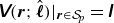 ${\unicode{x1D651}}(\boldsymbol{r};\hat{\boldsymbol{\ell} })|_{\boldsymbol{r}\in \mathcal{S}_{\!{p}}}={\unicode{x1D644}}$
. The volume term can be neglected in this large-screening limit, and we find
${\unicode{x1D651}}(\boldsymbol{r};\hat{\boldsymbol{\ell} })|_{\boldsymbol{r}\in \mathcal{S}_{\!{p}}}={\unicode{x1D644}}$
. The volume term can be neglected in this large-screening limit, and we find
 \begin{equation} \boldsymbol{\mu }^{{tE}}({\hat{\boldsymbol{\ell} }})=-\varepsilon \varPsi _0\int _{\mathcal{S}_{\!{p}}}{\rm d}S\, \boldsymbol{\mu }^{{tt}}(\hat {\boldsymbol{\ell }})\boldsymbol{\cdot }\left \{[\boldsymbol{\hat n}(\boldsymbol{r})\boldsymbol{\cdot }\boldsymbol{\nabla }]{\unicode{x1D651}}^{\kern1.5pt \top} (\boldsymbol{r};-{\hat{\boldsymbol{\ell} }})\right \}\boldsymbol{\cdot }\boldsymbol{\nabla }\boldsymbol{\varphi }(\boldsymbol{r}). \end{equation}
For a sphere $\boldsymbol{\hat n}=-\boldsymbol{\hat r}$
and after using (4.4), we find that (4.7) simplifies to
$\boldsymbol{\hat n}=-\boldsymbol{\hat r}$
and after using (4.4), we find that (4.7) simplifies to
 \begin{equation} \boldsymbol{\mu }^{{tE}}({\hat{\boldsymbol{\ell} }})=-6\pi \varepsilon a^2\varPsi _0\left [\frac {\partial }{\partial r}\overline {\mathcal{L}_0{\unicode{x1D642}}(\boldsymbol{r};\hat{\boldsymbol{\ell} })\boldsymbol{\cdot }({\unicode{x1D644}}-\boldsymbol{\hat r}\boldsymbol{\hat r})}\right ]_{r=a}. \end{equation}
Here, we denote a surface average over the unit sphere $S^2$
as
$S^2$
as $\overline {(\ldots )}=(4\pi )^{-1}\int _{S^2}{\rm d}^2\boldsymbol{\hat r}\, (\ldots )$
. Now, for fixed
$\overline {(\ldots )}=(4\pi )^{-1}\int _{S^2}{\rm d}^2\boldsymbol{\hat r}\, (\ldots )$
. Now, for fixed $\alpha$
, we may view
$\alpha$
, we may view $\mathcal{L}_0G_{\alpha \beta }(\boldsymbol{r};\hat{\boldsymbol{\ell} })$
as an incompressible vector field that is constant on
$\mathcal{L}_0G_{\alpha \beta }(\boldsymbol{r};\hat{\boldsymbol{\ell} })$
as an incompressible vector field that is constant on $\mathcal{S}_{\!{p}}$
. Therefore, its normal component has a vanishing gradient on
$\mathcal{S}_{\!{p}}$
. Therefore, its normal component has a vanishing gradient on $\mathcal{S}_{\!{p}}$
, which means that
$\mathcal{S}_{\!{p}}$
, which means that $({\partial }/{\partial r})\overline {\mathcal{L}_0{\unicode{x1D642}}(\boldsymbol{r};\hat{\boldsymbol{\ell} })\boldsymbol{\cdot }\boldsymbol{\hat r}\boldsymbol{\hat r}}$
vanishes on
$({\partial }/{\partial r})\overline {\mathcal{L}_0{\unicode{x1D642}}(\boldsymbol{r};\hat{\boldsymbol{\ell} })\boldsymbol{\cdot }\boldsymbol{\hat r}\boldsymbol{\hat r}}$
vanishes on $\mathcal{S}_{\!{p}}$
. The remaining part equals
$\mathcal{S}_{\!{p}}$
. The remaining part equals $-1/a$
upon using (A2); see Appendix A. We find
$-1/a$
upon using (A2); see Appendix A. We find $\boldsymbol{\mu }^{{tE}}({\hat{\boldsymbol{\ell} }})=6\pi \varepsilon a\varPsi _0\,\boldsymbol{\mu }^{{tt}}(\hat{\boldsymbol{\ell} })$
with components
$\boldsymbol{\mu }^{{tE}}({\hat{\boldsymbol{\ell} }})=6\pi \varepsilon a\varPsi _0\,\boldsymbol{\mu }^{{tt}}(\hat{\boldsymbol{\ell} })$
with components
 \begin{equation} \boldsymbol{\mu }^{{tE}}({\hat{\boldsymbol{\ell} }}) =\frac {\varepsilon }{\eta _{{s}}}\varPsi _0\left [m_\parallel (\gamma )\,\hat{\boldsymbol{\ell} }\hat{\boldsymbol{\ell} }+m_\perp (\gamma )\,({\unicode{x1D644}}-\hat{\boldsymbol{\ell} }\hat{\boldsymbol{\ell} })+m_{{o}}(\gamma )\,(\boldsymbol{\epsilon }\boldsymbol{\cdot }\hat{\boldsymbol{\ell} })\right ] \!, \quad \kappa a\gg 1. \end{equation}
Note that this result is not necessarily restricted to the case $|e\varPsi _0/(k_{{B}}T)|\ll 1$
, since it also applies to particles with a local radius of curvature much larger than
$|e\varPsi _0/(k_{{B}}T)|\ll 1$
, since it also applies to particles with a local radius of curvature much larger than $\kappa ^{-1}$
. Furthermore, we retrieve the Newtonian result for the Smoluchowski limit when
$\kappa ^{-1}$
. Furthermore, we retrieve the Newtonian result for the Smoluchowski limit when $\gamma \rightarrow 0$
. Interestingly, the fluid anisotropy still persists in
$\gamma \rightarrow 0$
. Interestingly, the fluid anisotropy still persists in $\boldsymbol{\mu }^{{tE}}({\hat{\boldsymbol{\ell} }})$
even for short Debye screening lengths. This is in sharp contrast to charged anisotropic particles in isotropic Newtonian fluids, where the electrophoretic mobility is isotropic and independent of particle shape under the same screening conditions.
$\boldsymbol{\mu }^{{tE}}({\hat{\boldsymbol{\ell} }})$
even for short Debye screening lengths. This is in sharp contrast to charged anisotropic particles in isotropic Newtonian fluids, where the electrophoretic mobility is isotropic and independent of particle shape under the same screening conditions.
4.3. Henry approximation
Next, we analyse electrophoresis for intermediate Debye screening length and small zeta potentials. Combining (4.1) and (4.4) gives
 \begin{equation} \boldsymbol{\mu }^{{tE}}(\hat {\boldsymbol{\ell }})=\varepsilon \int _{\mathcal{V}_{\!{f}}}\mathrm{d}V\, {\nabla} ^2\psi ^{{eq}}(r)\,[\mathcal{L}_0{\unicode{x1D642}}(\boldsymbol{r};\hat {\boldsymbol{\ell }})-\boldsymbol{\mu }^{{tt}}(\hat {\boldsymbol{\ell }})]\boldsymbol{\cdot }\boldsymbol{\nabla }\boldsymbol{\varphi }(\boldsymbol {r}). \end{equation}
We write $\int _{\mathcal{V}_{\!{f}}}\mathrm{d}V=\int _a^\infty \mathrm{d}r\, r^2\int _{S^2}{d}^2\boldsymbol{\hat r}$
, and we obtain
$\int _{\mathcal{V}_{\!{f}}}\mathrm{d}V=\int _a^\infty \mathrm{d}r\, r^2\int _{S^2}{d}^2\boldsymbol{\hat r}$
, and we obtain
 \begin{equation} \boldsymbol{\mu }^{{tE}}(\hat {\boldsymbol{\ell }})=4\pi \varepsilon \kappa ^2a\varPsi _0\int _a^\infty {\rm d}r\, r\text{e}^{\kappa (a-r)}\left \{\,\overline {[\mathcal{L}_0{\unicode{x1D642}}(\boldsymbol {r};\hat {\boldsymbol{\ell }})]\boldsymbol{\cdot }\boldsymbol{\nabla }\boldsymbol{\varphi }(\boldsymbol { r})}+\boldsymbol{\mu }^{{tt}}(\hat {\boldsymbol{\ell }})\right \}\!, \end{equation}
where we used that $\overline {\boldsymbol{\nabla }\boldsymbol{\varphi }(\boldsymbol{r})}=-{\unicode{x1D644}}$
. After applying the results from (A2) and (A10) (see Appendix A), we find
$\overline {\boldsymbol{\nabla }\boldsymbol{\varphi }(\boldsymbol{r})}=-{\unicode{x1D644}}$
. After applying the results from (A2) and (A10) (see Appendix A), we find
 \begin{equation} \overline {\mathcal{L}_0{\unicode{x1D642}}(\boldsymbol{r};\hat {\boldsymbol{\ell }})\boldsymbol{\cdot }\boldsymbol{\nabla }\boldsymbol{\varphi }(\boldsymbol { r})}=\left (-\frac {a}{r}+\frac {a^4}{4r^4}-\frac {a^6}{4r^6}\right )\boldsymbol{\mu }^{{tt}}(\hat {\boldsymbol{\ell }}). \end{equation}
We conclude that $\boldsymbol{\mu }^{{tE}}(\hat {\boldsymbol{\ell }})=6\pi \varepsilon a\varPsi _0f(\kappa a)\,\boldsymbol{\mu }^{{tt}}(\hat {\boldsymbol{\ell }})$
, with components
$\boldsymbol{\mu }^{{tE}}(\hat {\boldsymbol{\ell }})=6\pi \varepsilon a\varPsi _0f(\kappa a)\,\boldsymbol{\mu }^{{tt}}(\hat {\boldsymbol{\ell }})$
, with components
 \begin{gather} \boldsymbol{\mu }^{{tE}}(\hat {\boldsymbol{\ell }})=\frac {\varepsilon }{\eta _{{s}}}f(\kappa a)\,\varPsi _0\left [m_\parallel (\gamma )\,\hat{\boldsymbol{\ell} }\hat{\boldsymbol{\ell} }+m_\perp (\gamma )\,({\unicode{x1D644}}-\hat{\boldsymbol{\ell} }\hat{\boldsymbol{\ell} })+m_{{o}}(\gamma )\,(\boldsymbol{\epsilon }\boldsymbol{\cdot }\hat{\boldsymbol{\ell} })\right ] \!, \end{gather}
and the Henry function $f$
(Henry Reference Henry1931) defined by
$f$
(Henry Reference Henry1931) defined by
 \begin{equation} f(x)=\frac {2}{3}x^2\text{e}^x\int _1^\infty {\rm d}t\, t\text{e}^{-xt}\left (1-\frac {1}{t}+\frac {1}{4t^4}-\frac {1}{4t^6}\right )=1-\text{e}^x[5E_7(x)-2E_5(x)], \end{equation}
for $x\gt 0$
. Here,
$x\gt 0$
. Here, $E_{{k}}(x)=x^{{k}-1}\int _x^\infty {\rm d}t\, {\text{e}^{-t}}/{t^{{k}}}$
are exponential integrals. The function
$E_{{k}}(x)=x^{{k}-1}\int _x^\infty {\rm d}t\, {\text{e}^{-t}}/{t^{{k}}}$
are exponential integrals. The function $f$
has the properties
$f$
has the properties $\lim _{x\rightarrow 0}f(x)=2/3$
and
$\lim _{x\rightarrow 0}f(x)=2/3$
and $\lim _{x\rightarrow \infty }f(x)=1$
. Therefore, (4.13) reproduces both the Hückel limit (4.6), for
$\lim _{x\rightarrow \infty }f(x)=1$
. Therefore, (4.13) reproduces both the Hückel limit (4.6), for $\kappa a\ll 1$
, and the Smoluchowski limit (4.9), for
$\kappa a\ll 1$
, and the Smoluchowski limit (4.9), for $\kappa a\gg 1$
. The result for a Newtonian fluid is retrieved for
$\kappa a\gg 1$
. The result for a Newtonian fluid is retrieved for $\gamma \rightarrow 0$
as well. Again, the electrophoretic mobility tensor contains distinct parallel, perpendicular and axial components, while the modification by the Henry function is identical to that in isotropic Newtonian fluids. We note that for
$\gamma \rightarrow 0$
as well. Again, the electrophoretic mobility tensor contains distinct parallel, perpendicular and axial components, while the modification by the Henry function is identical to that in isotropic Newtonian fluids. We note that for $\gamma \ll 1$
,
$\gamma \ll 1$
, $m_{\perp ,\parallel }(\gamma )=O(\gamma ^2)$
, while
$m_{\perp ,\parallel }(\gamma )=O(\gamma ^2)$
, while $m_{{o}}(\gamma )=\gamma /2+O(\gamma ^3)$
(Everts & Cichocki Reference Everts and Cichocki2024a
). In this regime, the linear growth of the axial component of
$m_{{o}}(\gamma )=\gamma /2+O(\gamma ^3)$
(Everts & Cichocki Reference Everts and Cichocki2024a
). In this regime, the linear growth of the axial component of $\boldsymbol{\mu }^{{tE}}(\hat{\boldsymbol{\ell} })$
with
$\boldsymbol{\mu }^{{tE}}(\hat{\boldsymbol{\ell} })$
with $\gamma$
, which is proportional to the steady-state intrinsic rotation-rate vector of the fluid particles (Markovich & Lubensky Reference Markovich and Lubensky2021), is an important experimental signature of odd electrophoresis.
$\gamma$
, which is proportional to the steady-state intrinsic rotation-rate vector of the fluid particles (Markovich & Lubensky Reference Markovich and Lubensky2021), is an important experimental signature of odd electrophoresis.
We have also obtained (4.13) from a numerical computation using (4.1), (4.3) and (4.5), with the exact closed-form solution for ${\unicode{x1D651}}(\boldsymbol{r};\hat {\boldsymbol{\ell }})$
listed in Meissner-Oszer et al. (Reference Meissner-Oszer, Cichocki and Everts2026). Considering the complicated analytical form of this quantity shows the power of the singularity representation (4.4): it showcases how numerics can be completely circumvented due to the uncharged translating sphere having constant tractions on its surface. By the same properties, we find the remarkable result that
${\unicode{x1D651}}(\boldsymbol{r};\hat {\boldsymbol{\ell }})$
listed in Meissner-Oszer et al. (Reference Meissner-Oszer, Cichocki and Everts2026). Considering the complicated analytical form of this quantity shows the power of the singularity representation (4.4): it showcases how numerics can be completely circumvented due to the uncharged translating sphere having constant tractions on its surface. By the same properties, we find the remarkable result that $\boldsymbol{\mu }^{{tE}}(\hat{\boldsymbol{\ell} })$
is proportional to
$\boldsymbol{\mu }^{{tE}}(\hat{\boldsymbol{\ell} })$
is proportional to $\boldsymbol{\mu }^{{tt}}(\hat{\boldsymbol{\ell} })$
for a charged sphere within the Henry approximation and/or Smoluchowski limit.
$\boldsymbol{\mu }^{{tt}}(\hat{\boldsymbol{\ell} })$
for a charged sphere within the Henry approximation and/or Smoluchowski limit.
5. Conclusions and outlook
Our paper provides an exact analytical solution for the electrophoretic mobility of a charged spherical particle suspended in an electrolyte solution with odd viscosity. We have introduced, for the first time, the concept of a charged chiral active fluid, and generalised the expressions for the electrophoresis of arbitrarily shaped particles dissolved in an odd fluid. We explicitly calculated the electrophoretic mobility tensor for spherical particles dissolved in fluids with odd viscosity for low zeta potentials, small external electric fields, and general Debye screening length. Moreover, our results are valid for arbitrary values of the odd-viscosity coefficient. As in isotropic Newtonian fluids, we find no electrorotation for a homogeneously charged sphere, and find that the (translational) electrophoretic mobility of a sphere is proportional to the translational mobility of an uncharged sphere multiplied by the Henry function. Furthermore, we provide closed-form analytical expressions for both the Hückel and Smoluchowski limits. Our work demonstrates that odd viscosity leads to directional asymmetries in the electrophoretic mobility tensor, suggesting mechanisms for active control of charged colloidal motion in systems where odd viscosity is prevalent. Furthermore, these anisotropies are still present in the Smoluchowski limit. Thus our work bridges the gap between classical electrophoresis and odd fluids.
In our theoretical framework, we focused on the regime of linear electrophoresis, where we expanded around equilibrium for small external electric fields. Subsequently, we used a low zeta-potential approximation. Furthermore, we have assumed that the dielectric properties are isotropic. Relaxing these assumptions may lead to effects that are absent from the present analysis. For example, it is well known that a non-uniform equilibrium zeta potential can cause electrorotation of a charged particle in an isotropic Newtonian fluid – even within the Smoluchowski limit (Teubner Reference Teubner1982). It would be interesting to see whether this effect can also occur for a particle with uniform zeta potential in an anisotropic dielectric medium, where the anisotropy originates from a non-vanishing spin-momentum of the fluid. In general, dielectric anisotropy causes the surface charge to be inhomogeneous for a constant-potential particle, as one can deduce from equilibrium calculations of charged (colloidal) spheres in ion-doped nematic fluids (Everts et al. Reference Everts, Senyuk, Mundoor, Ravnik and Smalyukh2021). We expect that an odd (axial) dielectric contribution could generate analogous effects, leading to electrorotation through the coupling of induced surface-charge multipoles to an external electric field.
Alternatively, at high zeta potentials, $|e\varPsi _0/(k_{{B}}T)| \gg 1$
, we hypothesise that similar effects can occur through significant surface conduction and polarisation effects (Dukhin Reference Dukhin1993), which are not included in our present work. Other possible directions for future work include the extension of our analysis to multiple charged particles to assess the role of (odd) hydrodynamic interactions (Yuan & Olvera de la Cruz Reference Yuan and Olvera de la Cruz2023) on odd electrophoresis. It would be interesting to see how many-body effects will alter the results presented in this work, and how they differ from the isotropic Newtonian case (Chen & Keh Reference Chen and Keh1988).
$|e\varPsi _0/(k_{{B}}T)| \gg 1$
, we hypothesise that similar effects can occur through significant surface conduction and polarisation effects (Dukhin Reference Dukhin1993), which are not included in our present work. Other possible directions for future work include the extension of our analysis to multiple charged particles to assess the role of (odd) hydrodynamic interactions (Yuan & Olvera de la Cruz Reference Yuan and Olvera de la Cruz2023) on odd electrophoresis. It would be interesting to see how many-body effects will alter the results presented in this work, and how they differ from the isotropic Newtonian case (Chen & Keh Reference Chen and Keh1988).
Acknowledgements
We thank J. Gamdzyk for insightful discussions.
Funding
We acknowledge funding from the National Science Centre, Poland, within the OPUS LAP grant no. 2024/55/I/ST3/00998.
Declaration of interests
The authors report no conflict of interest.
Appendix A
In this appendix, we explicitly compute $\overline {\mathcal{L}_0{\unicode{x1D642}}(\boldsymbol{r};\hat{\boldsymbol{\ell} })}$
and
$\overline {\mathcal{L}_0{\unicode{x1D642}}(\boldsymbol{r};\hat{\boldsymbol{\ell} })}$
and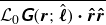 $\overline {\mathcal{L}_0{\unicode{x1D642}}(\boldsymbol{r};\hat{\boldsymbol{\ell} })\boldsymbol{\cdot }\boldsymbol{\hat r}\boldsymbol{\hat r}}$
, which were necessary to compute (4.8) and (4.12). Our starting point is that for stick boundary conditions, we have the single-layer integral representation theorem
$\overline {\mathcal{L}_0{\unicode{x1D642}}(\boldsymbol{r};\hat{\boldsymbol{\ell} })\boldsymbol{\cdot }\boldsymbol{\hat r}\boldsymbol{\hat r}}$
, which were necessary to compute (4.8) and (4.12). Our starting point is that for stick boundary conditions, we have the single-layer integral representation theorem
 \begin{equation} \boldsymbol{u}(\boldsymbol{r};\hat{\boldsymbol{\ell} })=\int _{\mathcal{S}_{\!{p}}}\mathrm{d}S\, {\unicode{x1D642}}(\boldsymbol{r}-\boldsymbol{r}';\hat{\boldsymbol{\ell} })\boldsymbol{\cdot }[\boldsymbol{\sigma }_{\!{H}}(\boldsymbol{r}')\boldsymbol{\cdot }\boldsymbol{\hat n}(\boldsymbol{r}')], \quad \boldsymbol{u}(\boldsymbol{r};\hat{\boldsymbol{\ell} })=\begin{cases} \boldsymbol{U}, & \boldsymbol{r}\in \mathcal{V}_{\!{p}},\\[3pt] \boldsymbol{v}(\boldsymbol{r};\hat{\boldsymbol{\ell} }),& \boldsymbol{r}\in \mathcal{V}_{\!{f}}, \end{cases} \end{equation}
where we only need the result for a translating sphere. In this case, the tractions $\boldsymbol{\sigma }_{\!{H}}(\boldsymbol{r}')\boldsymbol{\cdot }\boldsymbol{\hat n}(\boldsymbol{r}')$
are constant on
$\boldsymbol{\sigma }_{\!{H}}(\boldsymbol{r}')\boldsymbol{\cdot }\boldsymbol{\hat n}(\boldsymbol{r}')$
are constant on $\mathcal{S}_{\!{p}}$
and equal to
$\mathcal{S}_{\!{p}}$
and equal to $\boldsymbol{F}_{\!{H}}/(4\pi a^2)$
, as was proved by Everts & Cichocki (Reference Everts and Cichocki2024a
). Noting that the Green’s function can be written as
$\boldsymbol{F}_{\!{H}}/(4\pi a^2)$
, as was proved by Everts & Cichocki (Reference Everts and Cichocki2024a
). Noting that the Green’s function can be written as ${\unicode{x1D642}}(\boldsymbol{r};\hat{\boldsymbol{\ell} })=(a/r)\,{\unicode{x1D65C}}(\boldsymbol{\hat r};\hat{\boldsymbol{\ell} })$
(Everts & Cichocki Reference Everts and Cichocki2024a
), and evaluating (A1) for
${\unicode{x1D642}}(\boldsymbol{r};\hat{\boldsymbol{\ell} })=(a/r)\,{\unicode{x1D65C}}(\boldsymbol{\hat r};\hat{\boldsymbol{\ell} })$
(Everts & Cichocki Reference Everts and Cichocki2024a
), and evaluating (A1) for $\boldsymbol{r}=\boldsymbol{0}$
, we find that
$\boldsymbol{r}=\boldsymbol{0}$
, we find that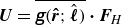 $\boldsymbol{U}=\overline {{\unicode{x1D65C}}(\boldsymbol{\hat r};\hat{\boldsymbol{\ell} })}\boldsymbol{\cdot }\boldsymbol{F}_{\!{H}}$
. We conclude that
$\boldsymbol{U}=\overline {{\unicode{x1D65C}}(\boldsymbol{\hat r};\hat{\boldsymbol{\ell} })}\boldsymbol{\cdot }\boldsymbol{F}_{\!{H}}$
. We conclude that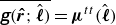 $\overline {{\unicode{x1D65C}}(\boldsymbol{\hat r};\hat{\boldsymbol{\ell} })}=\boldsymbol{\mu }^{{tt}}(\hat{\boldsymbol{\ell} })$
. Similar results are also noted by Khain et al. (Reference Khain, Fruchart, Scheibner, Witten and Vitelli2024). We now proceed to the computation of the relevant quantities.
$\overline {{\unicode{x1D65C}}(\boldsymbol{\hat r};\hat{\boldsymbol{\ell} })}=\boldsymbol{\mu }^{{tt}}(\hat{\boldsymbol{\ell} })$
. Similar results are also noted by Khain et al. (Reference Khain, Fruchart, Scheibner, Witten and Vitelli2024). We now proceed to the computation of the relevant quantities.
A.1. Computation of the surface average of $\mathcal{L}_0{\unicode{x1D642}}$
over
$S^2$
$\mathcal{L}_0{\unicode{x1D642}}$
over
$S^2$


First, we show that $\overline {({\nabla} ^2)^{{k}}{\unicode{x1D642}}(\boldsymbol{r};\hat{\boldsymbol{\ell} })}=0$
for
$\overline {({\nabla} ^2)^{{k}}{\unicode{x1D642}}(\boldsymbol{r};\hat{\boldsymbol{\ell} })}=0$
for ${{k}}\geq 1$
. We adopt spherical coordinates where
${{k}}\geq 1$
. We adopt spherical coordinates where $\hat{\boldsymbol{\ell} }$
is parallel to the
$\hat{\boldsymbol{\ell} }$
is parallel to the $z$
axis. In these coordinates, we decompose the Laplacian as
$z$
axis. In these coordinates, we decompose the Laplacian as ${\nabla} ^2={\nabla} _r^2+(1/r^2)\varDelta _{S^2}$
, where
${\nabla} ^2={\nabla} _r^2+(1/r^2)\varDelta _{S^2}$
, where ${\nabla} _r^2(\ldots )=(1/r^2)\,\partial _r^2[r^2(\ldots )]$
, and
${\nabla} _r^2(\ldots )=(1/r^2)\,\partial _r^2[r^2(\ldots )]$
, and $\varDelta _{S^2}$
is the Laplace–Beltrami operator on the unit sphere
$\varDelta _{S^2}$
is the Laplace–Beltrami operator on the unit sphere $S^2$
(Flanders Reference Flanders1963). It follows by direct computation that
$S^2$
(Flanders Reference Flanders1963). It follows by direct computation that ${\nabla} ^2{\unicode{x1D642}}(\boldsymbol{r};\hat{\boldsymbol{\ell} })=(a/r^3)\,\varDelta _{S^2}{\unicode{x1D65C}}(\boldsymbol{\hat r};\hat{\boldsymbol{\ell} })$
for
${\nabla} ^2{\unicode{x1D642}}(\boldsymbol{r};\hat{\boldsymbol{\ell} })=(a/r^3)\,\varDelta _{S^2}{\unicode{x1D65C}}(\boldsymbol{\hat r};\hat{\boldsymbol{\ell} })$
for $r\gt 0$
. The key step to proceed further is to observe that
$r\gt 0$
. The key step to proceed further is to observe that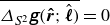 $\overline {\varDelta _{S^2}{\unicode{x1D65C}}(\boldsymbol{\hat r};\hat{\boldsymbol{\ell} })}=0$
, which can be shown by application of the divergence theorem on a curved manifold and noting that
$\overline {\varDelta _{S^2}{\unicode{x1D65C}}(\boldsymbol{\hat r};\hat{\boldsymbol{\ell} })}=0$
, which can be shown by application of the divergence theorem on a curved manifold and noting that $S^2$
is a compact manifold without boundary. We conclude that
$S^2$
is a compact manifold without boundary. We conclude that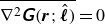 $\overline {{\nabla} ^2{\unicode{x1D642}}(\boldsymbol{r};\hat{\boldsymbol{\ell} })}=0$
for
$\overline {{\nabla} ^2{\unicode{x1D642}}(\boldsymbol{r};\hat{\boldsymbol{\ell} })}=0$
for $r\gt 0$
. Now suppose that the statement
$r\gt 0$
. Now suppose that the statement $\overline {({\nabla} ^2)^{{k}}{\unicode{x1D642}}(\boldsymbol{r};\hat{\boldsymbol{\ell} })}=0$
is true for
$\overline {({\nabla} ^2)^{{k}}{\unicode{x1D642}}(\boldsymbol{r};\hat{\boldsymbol{\ell} })}=0$
is true for ${{k}}={l}$
. Then
${{k}}={l}$
. Then $\overline {({\nabla} ^2)^{{l}+1}{\unicode{x1D642}}(\boldsymbol{r};\hat{\boldsymbol{\ell} })}={\nabla} _r^2[\overline {({\nabla} ^2)^{{l}}{\unicode{x1D642}}(\boldsymbol{r};\hat{\boldsymbol{\ell} })}]+(1/r^2)\,\overline {\varDelta _{S^2}[({\nabla} ^2)^{{l}}{\unicode{x1D642}}(\boldsymbol{r};\hat{\boldsymbol{\ell} })}]$
. The first term vanishes because of the induction hypothesis. The second term vanishes again by virtue of the divergence theorem on
$\overline {({\nabla} ^2)^{{l}+1}{\unicode{x1D642}}(\boldsymbol{r};\hat{\boldsymbol{\ell} })}={\nabla} _r^2[\overline {({\nabla} ^2)^{{l}}{\unicode{x1D642}}(\boldsymbol{r};\hat{\boldsymbol{\ell} })}]+(1/r^2)\,\overline {\varDelta _{S^2}[({\nabla} ^2)^{{l}}{\unicode{x1D642}}(\boldsymbol{r};\hat{\boldsymbol{\ell} })}]$
. The first term vanishes because of the induction hypothesis. The second term vanishes again by virtue of the divergence theorem on $S^2$
. This completes the proof of our initial statement. Now, using the linearity of the surface average, we obtain
$S^2$
. This completes the proof of our initial statement. Now, using the linearity of the surface average, we obtain
 \begin{equation} \overline {\mathcal{L}_0{\unicode{x1D642}}(\boldsymbol{r};\hat{\boldsymbol{\ell} })}=\overline {{\unicode{x1D642}}(\boldsymbol{r};\hat{\boldsymbol{\ell} })}=\frac {a}{r}\,\overline {{\unicode{x1D65C}}(\boldsymbol{\hat r};\hat{\boldsymbol{\ell} })}=\frac {a}{r}\,\boldsymbol{\mu }^{{tt}}(\hat{\boldsymbol{\ell} }) . \end{equation}
A.2. Computation of the surface average of
$\mathcal{L}_0{\unicode{x1D642}} \boldsymbol{\cdot }\boldsymbol{\hat r}\boldsymbol{\hat r}$
over
$S^2$


First, we show that $\overline {({\nabla} ^2)^k{\unicode{x1D642}}(\boldsymbol{r};\hat{\boldsymbol{\ell} })\boldsymbol{\cdot }\boldsymbol{\hat r}\boldsymbol{\hat r}}=0$
for
$\overline {({\nabla} ^2)^k{\unicode{x1D642}}(\boldsymbol{r};\hat{\boldsymbol{\ell} })\boldsymbol{\cdot }\boldsymbol{\hat r}\boldsymbol{\hat r}}=0$
for $k\geq 2$
. Because
$k\geq 2$
. Because $S^2$
is a compact manifold without boundary, we have the following Green’s identity for two tensors
$S^2$
is a compact manifold without boundary, we have the following Green’s identity for two tensors $\unicode{x1D63C}$
and
$\unicode{x1D63C}$
and $\unicode{x1D63D}$
defined on
$\unicode{x1D63D}$
defined on $S^2$
:
$S^2$
:
 \begin{equation} \overline {{\unicode{x1D63C}}(\boldsymbol{\hat r})\boldsymbol{\cdot }\varDelta _{S^2}{\unicode{x1D63D}}(\boldsymbol{\hat r})}=\overline {[\varDelta _{S^2}{\unicode{x1D63C}}(\boldsymbol{\hat r})]\boldsymbol{\cdot }{\unicode{x1D63D}}(\boldsymbol{\hat r})}. \end{equation}
Now take ${\unicode{x1D63C}}(\boldsymbol{\hat r})=\varDelta _{S^2}{\unicode{x1D65C}}(\boldsymbol{\hat r};\hat{\boldsymbol{\ell} })$
and
${\unicode{x1D63C}}(\boldsymbol{\hat r})=\varDelta _{S^2}{\unicode{x1D65C}}(\boldsymbol{\hat r};\hat{\boldsymbol{\ell} })$
and ${\unicode{x1D63D}}(\boldsymbol{\hat r})=\boldsymbol{\hat r}\boldsymbol{\hat r}$
. This results in
${\unicode{x1D63D}}(\boldsymbol{\hat r})=\boldsymbol{\hat r}\boldsymbol{\hat r}$
. This results in
 \begin{equation} \overline {[\varDelta _{S^2}\varDelta _{S^2}{\unicode{x1D65C}}(\boldsymbol{\hat r};\hat{\boldsymbol{\ell} })]\boldsymbol{\cdot }\boldsymbol{\hat r}\boldsymbol{\hat r}}=-6\overline {[\varDelta _{S^2}{\unicode{x1D65C}}(\boldsymbol{\hat r};\hat{\boldsymbol{\ell} })]\boldsymbol{\cdot }\boldsymbol{\hat r}\boldsymbol{\hat r}}, \end{equation}
where we used the divergence theorem on $S^2$
, and
$S^2$
, and $\varDelta _{S^2}\boldsymbol{\hat r}\boldsymbol{\hat r}=2({\unicode{x1D644}}-3\boldsymbol{\hat r}\boldsymbol{\hat r})$
. Furthermore, by direct computation, we find
$\varDelta _{S^2}\boldsymbol{\hat r}\boldsymbol{\hat r}=2({\unicode{x1D644}}-3\boldsymbol{\hat r}\boldsymbol{\hat r})$
. Furthermore, by direct computation, we find
 \begin{equation} [{\nabla} ^2{\nabla} ^2{\unicode{x1D642}}(\boldsymbol{r};\hat{\boldsymbol{\ell} })]\boldsymbol{\cdot }\boldsymbol{\hat r}\boldsymbol{\hat r}=\frac {6a}{r^5}[\varDelta _{S^2}{\unicode{x1D65C}}(\boldsymbol{\hat r};\hat{\boldsymbol{\ell} })]\boldsymbol{\cdot }\boldsymbol{\hat r}\boldsymbol{\hat r}+\frac {a}{r^5}[\varDelta _{S^2}\varDelta _{S^2}{\unicode{x1D65C}}(\boldsymbol{\hat r};\hat{\boldsymbol{\ell} })]\boldsymbol{\cdot }\boldsymbol{\hat r}\boldsymbol{\hat r}. \end{equation}
By taking the average over $S^2$
of this equation and using (A4), we find
$S^2$
of this equation and using (A4), we find $\overline {[{\nabla} ^2{\nabla} ^2{\unicode{x1D642}}(\boldsymbol{r};\hat{\boldsymbol{\ell} })]\boldsymbol{\cdot }\boldsymbol{\hat r}\boldsymbol{\hat r}}=0$
. The statement then follows by induction using steps similar to those in § A.1.
$\overline {[{\nabla} ^2{\nabla} ^2{\unicode{x1D642}}(\boldsymbol{r};\hat{\boldsymbol{\ell} })]\boldsymbol{\cdot }\boldsymbol{\hat r}\boldsymbol{\hat r}}=0$
. The statement then follows by induction using steps similar to those in § A.1.
Now we proceed with the computation of the remaining terms. It follows from the above that
 \begin{equation} \overline {[\mathcal{L}_0{\unicode{x1D642}}(\boldsymbol{r};\hat{\boldsymbol{\ell} })]\boldsymbol{\cdot }\boldsymbol{\hat r}\boldsymbol{\hat r}}=\overline {\left [\left (1+\frac {a^2}{6}{\nabla} ^2\right ){\unicode{x1D642}}(\boldsymbol{r};\hat{\boldsymbol{\ell} })\right ]\boldsymbol{\cdot }\boldsymbol{\hat r}\boldsymbol{\hat r}}. \end{equation}
To obtain the first term in (A6), we find by explicit calculation in spherical coordinates and partial integration that
 \begin{equation} \overline {[\boldsymbol{\nabla }\boldsymbol{\cdot }{\unicode{x1D642}}^{\top} (\boldsymbol{r};\hat{\boldsymbol{\ell} })]\boldsymbol{\hat r}}=-\frac {a}{r^2}\,\overline {{\unicode{x1D65C}}(\boldsymbol{\hat r};\hat{\boldsymbol{\ell} })\boldsymbol{\cdot }({\unicode{x1D644}}-2\boldsymbol{\hat r}\boldsymbol{\hat r})}, \quad r\gt 0. \end{equation}
Using the incompressibility condition, it then follows that $\overline {{\unicode{x1D65C}}(\boldsymbol{\hat r};\hat{\boldsymbol{\ell} })\boldsymbol{\cdot }({\unicode{x1D644}}-2\boldsymbol{\hat r}\boldsymbol{\hat r})}=0$
. Application of this result gives
$\overline {{\unicode{x1D65C}}(\boldsymbol{\hat r};\hat{\boldsymbol{\ell} })\boldsymbol{\cdot }({\unicode{x1D644}}-2\boldsymbol{\hat r}\boldsymbol{\hat r})}=0$
. Application of this result gives
 \begin{equation} \overline {{\unicode{x1D642}}(\boldsymbol{r};\hat{\boldsymbol{\ell} })\boldsymbol{\cdot }\boldsymbol{\hat r}\boldsymbol{\hat r}}=\frac {a}{r}\,\overline {{\unicode{x1D65C}}(\boldsymbol{\hat r};\hat{\boldsymbol{\ell} })\boldsymbol{\cdot }\boldsymbol{\hat r}\boldsymbol{\hat r}}=\frac {a}{2r}\,\overline {{\unicode{x1D65C}}(\boldsymbol{\hat r};\hat{\boldsymbol{\ell} })}=\frac {a}{2r}\,\boldsymbol{\mu }^{{tt}}(\hat{\boldsymbol{\ell} }). \end{equation}
For the second term in (A6), we need to find $\overline {[{\nabla} ^2{\unicode{x1D642}}(\boldsymbol{r};\hat{\boldsymbol{\ell} })]\boldsymbol{\cdot }\boldsymbol{\hat r}\boldsymbol{\hat r}}=(a/r^3)\overline {[\varDelta _{S^2}{\unicode{x1D65C}}(\boldsymbol{\hat r};\hat{\boldsymbol{\ell} })]\boldsymbol{\cdot }\boldsymbol{\hat r}\boldsymbol{\hat r}}$
. This contribution is calculated by first evaluating (A6) for
$\overline {[{\nabla} ^2{\unicode{x1D642}}(\boldsymbol{r};\hat{\boldsymbol{\ell} })]\boldsymbol{\cdot }\boldsymbol{\hat r}\boldsymbol{\hat r}}=(a/r^3)\overline {[\varDelta _{S^2}{\unicode{x1D65C}}(\boldsymbol{\hat r};\hat{\boldsymbol{\ell} })]\boldsymbol{\cdot }\boldsymbol{\hat r}\boldsymbol{\hat r}}$
. This contribution is calculated by first evaluating (A6) for $r=a$
:
$r=a$
:
 \begin{equation} \overline {[\mathcal{L}_0{\unicode{x1D642}}(a\boldsymbol{\hat r};\hat{\boldsymbol{\ell} })]\boldsymbol{\cdot }\boldsymbol{\hat r}\boldsymbol{\hat r}}=\overline {{\unicode{x1D65C}}(\boldsymbol{\hat r};\hat{\boldsymbol{\ell} })\boldsymbol{\cdot }\boldsymbol{\hat r}\boldsymbol{\hat r}}+\frac {1}{6}\overline {[\varDelta _{S^2}{\unicode{x1D65C}}(\boldsymbol{\hat r};\hat{\boldsymbol{\ell} })]\boldsymbol{\cdot }\boldsymbol{\hat r}\boldsymbol{\hat r}}. \end{equation}
However, $\mathcal{L}_0{\unicode{x1D642}}(a\boldsymbol{\hat r};\hat{\boldsymbol{\ell} })=\boldsymbol{\mu }^{{tt}}(\hat{\boldsymbol{\ell} })$
and
$\mathcal{L}_0{\unicode{x1D642}}(a\boldsymbol{\hat r};\hat{\boldsymbol{\ell} })=\boldsymbol{\mu }^{{tt}}(\hat{\boldsymbol{\ell} })$
and $\overline {\boldsymbol{\hat r}\boldsymbol{\hat r}}=1/3$
. We conclude that
$\overline {\boldsymbol{\hat r}\boldsymbol{\hat r}}=1/3$
. We conclude that $\overline {[\varDelta _{S^2}{\unicode{x1D65C}}(\boldsymbol{\hat r};\hat{\boldsymbol{\ell} })]\boldsymbol{\cdot }\boldsymbol{\hat r}\boldsymbol{\hat r}}=-\boldsymbol{\mu }^{{tt}}(\hat{\boldsymbol{\ell} })$
, therefore
$\overline {[\varDelta _{S^2}{\unicode{x1D65C}}(\boldsymbol{\hat r};\hat{\boldsymbol{\ell} })]\boldsymbol{\cdot }\boldsymbol{\hat r}\boldsymbol{\hat r}}=-\boldsymbol{\mu }^{{tt}}(\hat{\boldsymbol{\ell} })$
, therefore $\overline {[{\nabla} ^2{\unicode{x1D642}}(\boldsymbol{r};\hat{\boldsymbol{\ell} })]\boldsymbol{\cdot }\boldsymbol{\hat r}\boldsymbol{\hat r}}=-(a/r^3)\,\boldsymbol{\mu }^{{tt}}(\hat{\boldsymbol{\ell} })$
. Combining with (A8) and insertion in (A6) gives
$\overline {[{\nabla} ^2{\unicode{x1D642}}(\boldsymbol{r};\hat{\boldsymbol{\ell} })]\boldsymbol{\cdot }\boldsymbol{\hat r}\boldsymbol{\hat r}}=-(a/r^3)\,\boldsymbol{\mu }^{{tt}}(\hat{\boldsymbol{\ell} })$
. Combining with (A8) and insertion in (A6) gives
 \begin{equation} \overline {\mathcal{L}_0{\unicode{x1D642}}(\boldsymbol{r};\hat{\boldsymbol{\ell} })\boldsymbol{\cdot }\boldsymbol{\hat r}\boldsymbol{\hat r}}=\left (\frac {a}{2r}-\frac {a^3}{6r^3}\right )\boldsymbol{\mu }^{{tt}}(\hat{\boldsymbol{\ell} }). \end{equation}
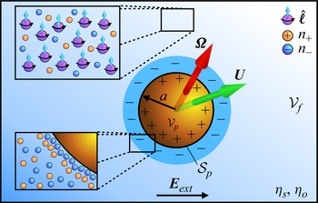
 a
a U
U Ω
Ω ηs
ηs ηo
ηo n+
n+ n−
n− Eext
Eext Vp
Vp Vf
Vf ℓ^
ℓ^
 Open access

