2.1. From DNS to independent diffuselets

In order to characterize the mixing properties of a flow, it is convenient to introduce a blob of scalar and to follow its advection, diffusion and mixing, a procedure easily carried out experimentally leading to global measures such as scalar variance, p.d.f.s of scalar, spectra, correlation functions and so on, and also to quantify the transient evolution of these quantities as a function of the flow structure, or location of deposition of the blob in heterogeneous flows. Numerically, this procedure is also possible by solving the diffusion–advection equation

(2.1)\begin{equation} \frac{\partial c}{\partial t} + \boldsymbol{u} \boldsymbol\ {\cdot}\ \boldsymbol{\nabla} c = D \boldsymbol{\nabla}^{2} c \end{equation}

using DNS. An example is given in figure 1(a,b) where a strip of scalar is advected in a sine flow with random phases for a very small diffusivity $D=10^{-6}$ (see Appendix A for further information on the numerical scheme). In some places, the strip is highly stretched such that its thickness decreases until it reaches the Batchelor scale $\sqrt {D/\gamma }$ at which diffusion starts to operate ($\gamma$ being the stretching rate). For small diffusivities, the thicknesses are extremely small and require a very fine mesh. In this example, 8192 Fourier modes have been used in each direction, which requires a memory of 500 Mo. The CFD condition then imposes that the time step must also be very small. Such 2-D DNS are extremely expensive in terms of CPU time for small diffusivities. In three dimensions this method is extremely demanding even for moderate diffusivities and nearly impossible for small diffusivities.

Figure 1. Different numerical methods used to quantify the mixing properties of a 2-D sine flow of period 1 with $U=0.3$ and $D=10^{-6}$ from $t=0$ (a,c,e) to $t=15$ (b,d, f). (a,b) Direct numerical simulation with $8192$ Fourier modes in each direction. In (c,d) the initial concentration field is modelled as a strip defined by 1000 tracers advected using the DSM (Meunier & Villermaux Reference Meunier and Villermaux2010). In (e, f) nine independent diffuselets with initial orientation $\theta _i$ are advected as described in § 2.2.

In order to treat numerically the case of small diffusivities, the DSM has been proposed by Meunier & Villermaux (Reference Meunier and Villermaux2010). The blob of scalar is modelled as a strip containing Lagrangian tracers which are advected by the flow

(2.2)\begin{equation} \frac{\mathrm{d}\kern0.06em \boldsymbol{x}_i}{\mathrm{d} t} = \boldsymbol{u}(\boldsymbol{x}_i). \end{equation}

Each element of the strip $[\boldsymbol {x}_i \ \boldsymbol {x}_{i+1}]$ has a length $\delta \ell _i=|\boldsymbol {x}_{i+1}-\boldsymbol {x}_i|$ and a striation thickness $s_i$ given by the incompressibility

(2.3)\begin{equation} s_i=\frac{s_0 \ \delta \ell_0}{\delta \ell_i}, \end{equation}

where $s_0$ and $\delta \ell _0$ are the initial thickness and length of each strip element. In this paper we will assume that the strip has initially a Gaussian profile (for simplicity) with a maximal concentration equal to 1 (from dimensionalisation). The characteristics of the strip can then be calculated easily using the Ranz transform (Ranz Reference Ranz1979) for each tracer. Indeed, defining a dimensionless time $\tau _i(t)$ given by

(2.4)\begin{equation} \frac{\mathrm{d} \tau_i}{\mathrm{d} t} = \frac{4D}{s_i^{2}}, \quad \mathrm{with}\ \tau_i(t=0)=1, \end{equation}

the maximal concentration at $\boldsymbol {x}_i$ is equal to $C_i=\tau _i^{-1/2}$ and the diffusive thickness (i.e. the Batchelor length) is equal to $s_i\sqrt {\tau _i}$. Indeed, the transverse profile of scalar is governed by a simple diffusion equation

(2.5)\begin{equation} \frac{\partial c_i}{\partial \tau_i}=\frac{1}{4} \frac{\partial^{2} c_i}{\partial \xi_i^{2}} \end{equation}

for the new variables $(\xi _i=n_i/s_i,\tau _i)$, where $n_i$ is the coordinate normal to the strip element $[\boldsymbol {x}_i \boldsymbol {x}_{i+1}]$. The transverse profile is thus given by

(2.6)\begin{equation} c_i(n_i)= \frac{1}{\sqrt{\tau_i}} \exp({-n_i^{2}/(s_i^{2}\tau_i)}). \end{equation}

An example is plotted in figure 1(d) after 15 periods of the sine flow. The maximal concentration and the thickness of the strip indeed corresponds to those found numerically by DNS. The computation is done with only 1000 tracers such that the computation time is only three minutes whereas it lasts a few hours for the DNS on the same computer. In this figure the strip has been plotted as a simple line with a modulated thickness and colour. It is possible to reconstruct the total scalar field on a mesh, as done in Meunier & Villermaux (Reference Meunier and Villermaux2010). However, as mentioned earlier, the required mesh may become extremely fine when the diffusivity becomes small. Alternative methods have thus been developed in order to get the statistics (p.d.f., variance) and the spectra of the scalar field (see Meunier & Villermaux Reference Meunier and Villermaux2010).

Martínez-Ruiz et al. (Reference Martínez-Ruiz, Meunier, Favier, Duchemin and Villermaux2018) have generalized this 2-D method to three dimensions by considering diffusive surface elements rather than diffusive strip elements. The striation thickness is simply given by the incompressibility as

(2.7)\begin{equation} s_i=s_0\frac{\delta A_0}{\delta A_i} , \end{equation}

where $\delta A_i$ is the area of the surface element (being initially equal to $\delta A_0$). Defining the dimensionalised time $\tau _i(t)$ in the same way using (2.4) leads to the maximal concentration $C_i=\tau _i^{-1/2}$ and the diffusive thickness $s_i \sqrt {\tau _i}$.

However, dealing numerically with a sheet is much more complex than dealing with a strip since each surface element is connected to its neighbours in physical space, although this connection is not trivial in the structure of the numerical variables. Furthermore, refining the surface by adding surface elements, e.g. when the element's size or curvature is too large, adds another complexity. These complex techniques are necessary to reconstruct the shape of the sheet. Fortunately, they are not necessary to obtain the p.d.f. and the variance of scalar in the diluted limit, i.e. when there is no self-aggregation of the folded strip or sheet. Indeed, each element can be solved independently since the diffusion (2.1) is linear for the concentration. The variance and the p.d.f. are then found as an ensemble average over all elements. Each element is the response to an initial insertion of scalar with a given striation thickness and an infinitely small area. This surface element may be called the diffuselet. It corresponds to the Green function of a surface rather than a point.

For independent diffuselets, the main problem is to calculate the striation thickness of each element without knowing the position of the neighbours. Indeed, the stretching between neighbouring points was used previously to calculate the length (in two dimensions) or the area (in three dimensions) of the diffuselet. This is what we propose in the next section.

2.2. General equations for a diffuselet

We first illustrate the concepts and the kinematic construction of the relevant quantities involved in the general discussion in two dimensions. We then extend this construction to the 3-D case. We finally apply the Ranz transform to incorporate diffusion with kinematics.

2.2.1. Concepts and kinematic construction in two dimensions

Let $\delta \boldsymbol {\ell }=(\delta \ell _x,\delta \ell _y)$ be a vector of the plane $\{x,y\}$ between two material particles $\boldsymbol {x}_i$ and $\boldsymbol {x}_{i}+\delta \boldsymbol {\ell }$ advected by a velocity field $\boldsymbol u(\boldsymbol x,t)=(u,v)$, as sketched in figure 2. The kinematic transport of $\delta \boldsymbol {\ell }$ in (2.2) is such that $\dot {\delta \boldsymbol {\ell }}=\boldsymbol u(\boldsymbol x+\delta \boldsymbol \ell )-\boldsymbol u(\boldsymbol x)$ so that

(2.8)$$\begin{gather} \dot{\delta \ell}_x=\delta \ell_x\partial_xu+\delta \ell_y\partial_yu, \end{gather}$$

(2.9)$$\begin{gather}\dot{\delta \ell}_y=\delta \ell_x\partial_xv+\delta \ell_y\partial_yv \end{gather}$$

or, in compact form (Batchelor Reference Batchelor1952; Cocke Reference Cocke1969), $\dot {\boldsymbol {\ell }}=(\boldsymbol {\ell }\ {\cdot}\ \boldsymbol {\nabla })\boldsymbol u$, also equivalently written in terms of the velocity gradient tensor $\dot {\delta \boldsymbol {\ell }}=({\overline {\overline {{\boldsymbol\nabla} \boldsymbol{\mathsf{u}}}}})\, \delta \boldsymbol \ell$, where

(2.10)\begin{equation} {\overline{\overline{{\boldsymbol\nabla} \boldsymbol{\mathsf{u}}}}}= \begin{bmatrix} \partial_x u & \partial_y u \\ \partial_x v & \partial_y v \end{bmatrix},\text{ with transpose }{\overline{\overline{{\boldsymbol\nabla} \boldsymbol{\mathsf{u}}}}}^{{\star}}= \begin{bmatrix} \partial_x u & \partial_x v \\ \partial_y u & \partial_y v \end{bmatrix}. \end{equation}

The stretching factor of the segment $\delta \boldsymbol \ell$ or the pair dispersion rate of its extremities measured by $\delta \ell ^{2}=\delta \ell _x^{2}+\delta \ell _y^{2}=\delta \boldsymbol \ell ^{\star }\delta \boldsymbol \ell$ involves the operator ${\overline {\overline {{\boldsymbol\nabla} \boldsymbol{\mathsf{u}}}}}$.

Figure 2. Schematic of the evolution of a segment (a) and a surface (b) elongated by a flow $\boldsymbol u(\boldsymbol x)$. In two dimensions a blob with area $s_0 \delta \ell _0$ is elongated into a stripe of length $\delta \ell$ and transverse size $s$ so that $s \delta \ell \sim s_0 \delta \ell _0$. The iso-values of scalar denoted as blue lines are compressed. The concentration gradient across the stripe increases proportionally to $1/s$, i.e. to $\delta \ell$. the concentration gradient vector is thus proportional to $\delta \boldsymbol \ell ^{\perp }$. In three dimensions the same construction is valid for a blob of volume $s_0 \delta A_0$ such that the concentration gradient is proportional to $\delta \! \boldsymbol {A}^{\perp }$.

We now define a vector $\delta \boldsymbol \ell ^{\perp }$ normal to $\delta \boldsymbol {\ell }$ with the same norm. This vector is simply $\delta \boldsymbol \ell ^{\perp }=(\delta \ell _y,- \delta \ell _x)$ and its dynamics obeys

(2.11)\begin{equation} \frac{\mathrm{d} \delta \boldsymbol \ell^{{\perp}}}{ \mathrm{d} t}={-}({\overline{\overline{{\boldsymbol\nabla} \boldsymbol{\mathsf{u}}}}}^{{\star}})\delta \boldsymbol \ell^{{\perp}}+(\boldsymbol{\nabla} \boldsymbol\ {\cdot}\ \boldsymbol{u})\delta \boldsymbol \ell^{{\perp}}, \end{equation}

where $\boldsymbol {\nabla } \ {\cdot}\ \boldsymbol {u}=(\partial _x u,\partial _yv)$ is the flow divergence. For incompressible motions with $\boldsymbol {\nabla } \ {\cdot}\ \boldsymbol {u}=0$, we simply have $\dot {\delta \boldsymbol \ell ^{\perp }}=-({\overline {\overline {{\boldsymbol\nabla} \boldsymbol{\mathsf{u}}}}}^{\star })\delta \boldsymbol \ell ^{\perp }$.

The norm of $\delta \boldsymbol \ell ^{\perp }$ intensifies when the length $\delta \ell$ of the segment increases. In an incompressible flow this stretching of $\delta \ell$ implies that the lines parallel to the stripe get closer (as depicted by blue lines in figure 2). It leads to an intensification of the gradient of a passive substance in the direction normal to it, that is, in the direction of $\delta \boldsymbol \ell ^{\perp }$. For instance, if a blob with area $\delta \ell _0 s_0$ and concentration $c$ elongates into a stripe of length $\delta \ell$ and transverse size $s$ so that $\delta \ell \sim \delta \ell _0 \ s_0/s$, as in figure 2, the concentration gradient across the stripe $c/s$ first increases proportionally to the norm $\delta \ell$ of the vector $\delta \boldsymbol \ell ^{\perp }$, before being smeared out by diffusion. It is therefore natural, as first underlined by Corrsin (Reference Corrsin1953) and later Brethouwer, Hunt & Nieuwstadt (Reference Brethouwer, Hunt and Nieuwstadt2003), to find the operator $- {\overline {\overline {{\boldsymbol\nabla} \boldsymbol{\mathsf{u}}}}}^{\star }$ instead of ${\overline {\overline {{\boldsymbol\nabla} \boldsymbol{\mathsf{u}}}}}$ in the evolution equation of scalar gradients (see also Batchelor & Townsend (Reference Batchelor and Townsend1956) and Ertel (Reference Ertel1942) in related contexts),

(2.12)\begin{equation} \frac{\mathrm{d} \,\boldsymbol{\nabla} c}{\mathrm{d} t} ={-} {\overline{\overline{{\boldsymbol\nabla} \boldsymbol{\mathsf{u}}}}}^{{\star}} (\boldsymbol{\nabla} c) + D\boldsymbol{\nabla}^{2} (\boldsymbol{\nabla} c). \end{equation}

As also noted by Corrsin (Reference Corrsin1953), this equation differs from the vorticity equation since the scalar gradient is a lamellar vector (i.e. $\boldsymbol {\nabla } \times (\boldsymbol {\nabla } c) = 0$) whereas the vorticity is solenoidal (i.e. $\boldsymbol {\nabla } \ {\cdot}\ \omega =0$). In a Fourier decomposition of the scalar concentration field this operator also governs the wavevectors norm (see equation (2.5) in Kraichnan Reference Kraichnan1974).

2.2.2. Extension to three dimensions

Let us consider a surface element of area $\delta \! A_i$ normal to the unit vector ${\boldsymbol n_i}$ at a position $\boldsymbol {x}_i$ and at time $t$ (see figure 2). We define, as above, the surface vector $\delta \! \boldsymbol {A}_i = \delta \! A_i {\boldsymbol n}_i$, initially equal to $\delta \! \boldsymbol {A}_0$. The norm of $\delta \! \boldsymbol {A}_i$ is proportional to the surface area $\delta \! A_i$. Since $\delta \! \boldsymbol {A}_i$ is normal to the surface, it follows the same evolution as $\delta \boldsymbol \ell$ in two dimensions that was governed by (2.11). Indeed, it can be shown by assuming that $\delta \! \boldsymbol {A}_i$ is the cross-product of two tangential vectors ${\boldsymbol t}_1 \times {\boldsymbol t}_2$ that

(2.13)\begin{align} \frac{\mathrm{d} \, \delta \! \boldsymbol{A}_i}{\mathrm{d} t} &= \frac{\mathrm{d}{\boldsymbol t}_1}{\mathrm{d} t} \times {\boldsymbol t}_2 + {\boldsymbol t}_1 \times \frac{\mathrm{d}{\boldsymbol t}_2}{\mathrm{d} t} \end{align}

(2.14)\begin{align} &= ({\overline{\overline{{\boldsymbol\nabla} \boldsymbol{\mathsf{u}}}}}\,{\boldsymbol t}_1) \times {\boldsymbol t}_2+{\boldsymbol t}_1 \times ({\overline{\overline{{\boldsymbol\nabla} \boldsymbol{\mathsf{u}}}}}\,{\boldsymbol t}_2) \end{align}

(2.15)\begin{align} &={-} {\overline{\overline{{\boldsymbol\nabla} \boldsymbol{\mathsf{u}}}}}^{{\star}} ({\boldsymbol t}_1 \times {\boldsymbol t}_2)+(\boldsymbol{\nabla} \boldsymbol\ {\cdot}\ \boldsymbol{u}) ({\boldsymbol t}_1 \times {\boldsymbol t}_2) \end{align}

(2.16)\begin{align} &={-} {\overline{\overline{{\boldsymbol\nabla} \boldsymbol{\mathsf{u}}}}}^{{\star}} \delta \! \boldsymbol{A}_i +(\boldsymbol{\nabla} \boldsymbol\ {\cdot}\ \boldsymbol{u}) \, \delta \! \boldsymbol{A}_i, \end{align}

where ${\overline {\overline {{\boldsymbol\nabla} \boldsymbol{\mathsf{u}}}}}^{\star }(\boldsymbol {x}_i,t)$ is the transpose of the velocity gradient tensor ${\overline {\overline {{\boldsymbol\nabla} \boldsymbol{\mathsf{u}}}}}(\boldsymbol {x}_i,t)$ such that

(2.17)\begin{equation} {\overline{\overline{{\boldsymbol\nabla} \boldsymbol{\mathsf{u}}}}}= \begin{bmatrix} \partial_x u & \partial_y u & \partial_z u\\ \partial_x v & \partial_y v & \partial_z v\\ \partial_x w & \partial_y w & \partial_z w \end{bmatrix},\text{ giving }{\overline{\overline{{\boldsymbol\nabla} \boldsymbol{\mathsf{u}}}}}^{{\star}}= \begin{bmatrix} \partial_x u & \partial_x v & \partial_x w\\ \partial_y u & \partial_y v & \partial_y w\\ \partial_z u & \partial_z v & \partial_z w \end{bmatrix}. \end{equation}

For an incompressible flow with $\boldsymbol {\nabla } \ {\cdot}\ \boldsymbol {u}=0$, the surface vector evolves according to the linear equation

(2.18)\begin{equation} \frac{\mathrm{d} \, \delta \! \boldsymbol{A}_i}{\mathrm{d} t}={-} {\overline{\overline{{\boldsymbol\nabla} \boldsymbol{\mathsf{u}}}}}^{{\star}} \, \delta \! \boldsymbol{A}_i. \end{equation}

As classically done for the study of pair dispersion, it is convenient to define the tensor $\boldsymbol{\mathsf{L}}_i(t)$ by

(2.19)\begin{equation} \frac{\mathrm{d} \boldsymbol{\mathsf{L}}_i}{\mathrm{d} t} ={-} {\overline{\overline{{\boldsymbol\nabla} \boldsymbol{\mathsf{u}}}}}^{{\star}} \boldsymbol{\mathsf{L}}_i,\quad \text{with} \ \boldsymbol{\mathsf{L}}_i(t=0)=\boldsymbol{\mathsf{I}}, \end{equation}

where ${\overline {\overline {{\boldsymbol\nabla} \boldsymbol{\mathsf{u}}}}}^{\star }$ is calculated at position $\boldsymbol {x}_i(t)$ and with $\boldsymbol{\mathsf{I}}$ the diagonal unit matrix. At time $t$, the surface vector is then equal to

(2.20)\begin{equation} \delta \! \boldsymbol{A}_i(t)= \boldsymbol{\mathsf{L}}_i(t) \delta \! \boldsymbol{A}_0. \end{equation}

The same solution holds in two dimensions for $\delta \boldsymbol \ell ^{\perp }(t)$.

2.2.3. Ranz transform

The striation thickness $s_i$ is explicit from (2.7) by replacing $\delta \!A_i^{2}=\delta \! \boldsymbol {A}_i^{\star }\delta \! \boldsymbol {A}_i$ with its solution (2.20),

(2.21)\begin{equation} s_i=s_0({\boldsymbol n^{{\star}}_0} \boldsymbol{\mathsf{L}}^{{\star}}\boldsymbol{\mathsf{L}} {\boldsymbol n_0})^{-{1}/{2}}, \end{equation}

whereas the time $\tau _i$ is given explicitly by introducing this formula into (2.4),

(2.22)\begin{equation} \tau_i={\boldsymbol n^{{\star}}_0} \boldsymbol{\mathsf{T}}_i {\boldsymbol n_0}, \end{equation}

where we have defined the operator

(2.23)\begin{equation} \boldsymbol{\mathsf{T}}_i=\boldsymbol{\mathsf{I}}+\frac{4D}{s_0^{2}} \int_0^{t} \boldsymbol{\mathsf{L}}_i^{{\star}} \boldsymbol{\mathsf{L}}_i \,{\rm d}t. \end{equation}

As before, the concentration profile across a diffuselet initially perpendicular to ${\boldsymbol n_0}$ is a Gaussian profile given by (2.6) with $s_i$ and $\tau _i$ given above. These formulae are obviously also valid in two dimensions with ${\boldsymbol n}_0$ being the unit vector perpendicular to the filamentary strip element.

Consider the 2-D sine flow as an example. The result is exactly similar to the one plotted in figure 1(d) when taking initially the diffuselets along the filament of figure 1(c). However, this method also works for independent diffuselets with arbitrary orientations $\theta _i$, as shown in figure 1(e). Defining the normal vector 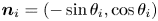${\boldsymbol n}_i=(-\sin \theta _i,\cos \theta _i)$ leads to the position, orientation, diffusive thickness and maximal concentration of the diffuselet after 15 iterations, as plotted in figure 1(e).

The final result so obtained is exactly the same as that given by Balkovsky & Fouxon (Reference Balkovsky and Fouxon1999) using the second momentum of scalar for an ellipsoidal blob with axes of initial length $2e^{\rho _{01}}$, $2e^{\rho _{02}}$ and $2e^{\rho _{03}}$. Assuming that the axis $e^{\rho _{3}}$ is much smaller than the two other axes, i.e. that the blob is a surface element, they find that the diffusive length is equal to $2e^{\rho _3}$ with $\rho _3$ given in their formula (2.5), where $\tilde {\sigma }_{33}$ is the compression rate along the smallest axis $\rho _3$. Although very different at first glance, their formula can be simplified into our formula by noting that $2e^{\rho _{03}}=s_0$ and that $\int \tilde {\sigma }_{33} \,\mathrm {d} t = \log (s_i/s_0)$. From their result, the diffusive thickness is equal to

(2.24)\begin{equation} 2 e^{\rho_3} = s_i \sqrt{1+\int_0^{t} \frac{4 D}{s_i^{2}}}, \end{equation}

which is identical to our result $s_i\sqrt {\tau _i}$ (see also de Rivas & Villermaux Reference de Rivas and Villermaux2016). The main problem in their derivation is that the compression rate $\tilde {\sigma }_{33}$ must be calculated in the local frame of reference aligned with the ellipsoid. Although theoretically possible, this rotation of the basis is difficult to do numerically. This is why our technique is simpler since the orientation of the surface is not required at each time.

It should be noted that the use of the tensors $\boldsymbol{\mathsf{L}}_i$ and $\boldsymbol{\mathsf{T}}_i$ is not required if each diffuselet is chosen with a unique initial orientation. Indeed, it would be possible to integrate (2.18) in time to get the surface vector $\delta \! \boldsymbol {A}_i$ from which $s_i$ and $\tau _i$ can be obtained. This would require the storage of seven variables (for $\boldsymbol {x}_i$, $\delta \! \boldsymbol {A}_i$ and $\tau _i$) instead of 18 (for $\boldsymbol {x}_i$, $\boldsymbol{\mathsf{L}}_i$ and the symmetric tensor $\tau _i$). However, using the tensors $\boldsymbol{\mathsf{L}}_i$ and $\boldsymbol{\mathsf{T}}_i$ permits us to vary a posteriori the orientation of the diffuselet. This helps to converge the statistics when calculating the p.d.f. of the scalar, as will be shown in the next section.

2.3. Statistics over the initial orientation of the diffuselet

Several quantities have been extensively studied in the context of mixing. In the absence of diffusion (i.e. for $D=0$), the stretching factor or the Lyapunov exponent are known to characaterize the properties of the flow. Generally, it is the stretching factor between two points which is calculated from the eigenvalues of the tensor $\boldsymbol{\mathsf{L}}_p^{\star} \boldsymbol{\mathsf{L}}_p$, where $\boldsymbol{\mathsf{L}}_p$ is the pair dispersion tensor solution of $\mathrm {d} \boldsymbol{\mathsf{L}}_p/\mathrm {d} t={\overline {\overline {{\boldsymbol\nabla} \boldsymbol{\mathsf{u}}}}}\,\boldsymbol{\mathsf{L}}_p$. In our case we are more interested by the stretching factor of the surfaces since it corresponds to the compression factor of the striation thickness, which governs the diffusion problem. As shown above, the stretching factor $\rho =\delta A_i/\delta A_0$ of a diffuselet is simply given by

(2.25)\begin{equation} \rho = ({\boldsymbol n^{{\star}}_0} \boldsymbol{\mathsf{L}}_i^{{\star}}\boldsymbol{\mathsf{L}}_i{\boldsymbol n_0})^{{1}/{2}}, \end{equation}

where ${\boldsymbol n}_0$ is the unit vector normal to the initial diffuselet. We now describe the 2-D and 3-D cases sequentially, in order to obtain concrete analytical formulae in each case.

2.3.1. Two-dimensional case

In two dimensions and for a given diffuselet $i$ at time $t$, the tensor $\boldsymbol{\mathsf{L}}_i^{\star } \boldsymbol{\mathsf{L}}_i$ is symmetric and its two eigenvalues are inverse because of the incompressibility. They are called $\mu _i$ and $\mu _i^{-1}$ with $\mu _i>1$. On the basis of the tensor $\boldsymbol{\mathsf{L}}_i^{\star } \boldsymbol{\mathsf{L}}_i$ the unit vector is taken as $\boldsymbol n_0=(\cos \theta,\sin \theta )$, with $\theta$ varying from 0 to ${\rm \pi} /2$. The stretching factor $\rho _i=\delta \ell _i/\delta \ell _0$ of the diffuselet is given by

(2.26)\begin{equation} \rho_i^{2} = \mu_i \cos^{2}\theta + \mu_i^{{-}1} \sin^{2} \theta. \end{equation}

The mean Lyapunov exponent $\bar {\lambda }_i = \langle \log \rho _i \rangle /t$ over all initial orientations can be calculated by averaging over $\theta$,

(2.27)\begin{equation} \bar{\lambda} = \frac{1}{t} \frac{1}{{\rm \pi}/2} \int_{\theta=0}^{{\rm \pi}/2} \frac{1}{2} \log (\mu_i \cos^{2}\theta + \mu_i^{{-}1} \sin^{2} \theta )\,\mathrm{d} \theta. \end{equation}

The integral can be calculated analytically, which leads to a simple expression for the mean Lyapunov exponent of all diffuselets

(2.28)\begin{equation} \bar{\lambda} = \frac{\langle \log \rho \rangle}{t} = \frac{1}{N t} \sum_{i=1}^{N} \log \left( \frac{1+\mu_i}{2 \sqrt{\mu_i}}\right). \end{equation}

Nevertheless, it is possible to get more information from the eigenvalues of the tensor $\boldsymbol{\mathsf{L}}_i$. Indeed, the p.d.f. of the stretching factor for this diffuselet satisfies

(2.29)\begin{equation} P_i(\rho) \,\mathrm{d} \rho = \frac{\mathrm{d} \theta}{{\rm \pi}/2}, \end{equation}

which can be written as $P_i(\rho )=2/({\rm \pi} \, \mathrm {d}\rho /\mathrm {d} \theta )$. Calculating $\mathrm {d} \rho /\mathrm {d} \theta$ and using the fact that $\cos ^{2}\theta =(\rho ^{2}-\mu _i^{-1})/(\mu _i-\mu _i^{-1})$ and $\sin ^{2}\theta =(\mu _i-\rho ^{2})/(\mu _i-\mu _i^{-1})$ leads to

(2.30)\begin{equation} P_i(\rho)=\frac{2 \rho}{{\rm \pi} \sqrt{\mu_i-\rho^{2}}\sqrt{\rho^{2}-\mu_i^{{-}1}}}, \end{equation}

with $\rho$ varying between $\mu _i^{-1}$ and $\mu _i$. Because the stretching factors often increase exponentially in time, it is more convenient to calculate the p.d.f. of $\log \rho$ using the fact that $P_i(\log \rho )=\rho P_i(\rho )$. This formula can then be averaged over the $N$ diffuselets to get the statistics of the stretching factor,

(2.31)\begin{equation} P(\log \rho)= \frac{1}{N} \sum_{i=1}^{N} \frac{2 \rho^{2}}{{\rm \pi} \sqrt{\mu_i-\rho^{2}}\sqrt{\rho^{2}-\mu_i^{{-}1}}}. \end{equation}

This p.d.f. of $\log \rho$ is plotted in figure 3(a) as red symbols for a 2-D sine flow. It is already well converged for only $N=1000$ diffuselets homogeneously distributed for $x$ and $y$ in $[0;1]$. This comes from the fact that each diffuselet incorporates all the orientations ${\boldsymbol n}_0$ at the same time thanks to the tensor $\boldsymbol{\mathsf{L}}_i$. If the calculation was done for a single orientation (i.e. by solving an equation for $\delta \! \boldsymbol {A}_i$ rather than for $\boldsymbol{\mathsf{L}}_i$), the p.d.f. would be obtained as the histogram of stretching factors $\rho _i$. This is what is plotted in figure 3(a) as blue symbols. It is clear that the number of diffuselets is not sufficient for the convergence of the p.d.f. It indicates that the use of the tensor $\boldsymbol{\mathsf{L}}_i$ is extremely efficient despite a slightly larger memory usage. The parabolic shape of the p.d.f. will be studied in detail in § 3 and compared with theoretical predictions.

Figure 3. Probability distribution function of the stretching rate (a) and scalar concentration (b) obtained for 1000 diffuselets in a 2-D sine flow after 50 iterations. The blue symbols correspond to a single initial orientation ${\boldsymbol n_0}$ along the $y$ axis whereas red symbols correspond to an ensemble average with ${\boldsymbol n_0}$ taking all orientations, as given by (2.31) and (2.38).

The strength of the diffuselet method is that the scalar field around each tracer is known quantitatively. The variance of concentration can be calculated analytically for each diffuselet and then averaged when the initial orientation is varied. As a first step, it is interesting to model the Gaussian transverse profile by a top-hat profile with maximal concentration $C_i=1/\sqrt {\tau _i}$, diffusive thickness $s_i \sqrt {\tau _i}$ and length $\delta \ell _0 s_0 / s_i$. Thus, this rectangular diffuselet has an area $\delta \ell _0 s_0 \sqrt {\tau _i}$ that is equal to $\delta \ell _0 s_0/C_i$. We can check here that the total quantity of scalar ($C_i$ $\times$ initial area) is conserved with time. Each diffuselet has a variance $\int c^{2}(x,y) \,{{\rm d}\kern0.06em x} \,{{\rm d} y}$ equal to $C_i^{2}$ multiplied by its area. This variance is thus simply equal to $C_i \delta \ell _0 s_0$. The maximal concentration $C_i=1/\sqrt {\tau _i}$ can be written using (2.22),

(2.32)\begin{equation} C_i=(\eta_i \cos^{2} \theta + \eta'_i \sin^{2}\theta)^{{-}1/2}, \end{equation}

where $\eta _i>\eta '_i$ are the two positive eigenvalues of the symmetric tensor $\boldsymbol{\mathsf{T}}_i$ (by writing ${\boldsymbol n}_0=(\cos \theta,\sin \theta )$ on the basis of the eigenvectors). The mean variance is thus equal to

(2.33)\begin{equation} \langle c^{2} \rangle_{{top\text{-}hat}} = \frac{\delta\ell_0 s_0}{{\rm \pi}/2} \int_{\theta=0}^{{\rm \pi}/2} \frac{\mathrm{d} \theta}{[\eta_i \cos^{2}(\theta) + \eta'_i \sin^{2}(\theta)]^{1/2}}. \end{equation}

The integral can be computed analytically leading to a simple formula for the variance,

(2.34)\begin{equation} \langle c^{2} \rangle_{{top\text{-}hat}} = \frac{2 \delta\ell_0 s_0 K(1-\eta_i/\eta_i')}{{\rm \pi} \sqrt{\eta_i'}}, \end{equation}

with $K$ the complete elliptic integral of the first kind.

The variance $\int c^{2}(x,y) \,{{\rm d}\kern0.06em x} \,{{\rm d} y}$ for a Gaussian profile as in (2.6) can then be calculated easily since for each $\theta$ it is equal to the variance of the top-hat profile multiplied by $\sqrt {{\rm \pi} /2}$. Summing over all diffuselets, the total variance reads

(2.35)\begin{equation} \langle c^{2}\rangle=\frac{\sqrt{2}\delta\ell_0 s_0}{\sqrt{\rm \pi}} \sum_{i=1}^{N} \frac{K(1-\eta_i/\eta_i')}{\sqrt{\eta_i'}}. \end{equation}

For each diffuselet, the p.d.f. of concentration can also be calculated when varying the initial orientation of the diffuselet. As a first step, the top-hat profile is considered such that the contribution of each diffuselet to the p.d.f. at $C=C_i$ is proportional to its area $\delta \ell _0 s_0 / C_i$. The p.d.f. of maximal concentration thus contains two peaks at $C=0$ and $C=C_i$ for a single diffuselet with a single initial orientation. However, $C_i$ depends on the initial orientation according to (2.32). For each diffuselet, the p.d.f. of maximal concentration is given by

(2.36)\begin{equation} Q_i(C) \,\mathrm{d} C= \frac{s_0 \delta\ell_0}{C} \frac{\mathrm{d} \theta}{{\rm \pi}/2}, \end{equation}

with $\theta$ varying uniformly from $0$ to ${\rm \pi} /2$. Indeed, the initial orientation of the diffuselets is a priori random, with no privileged direction. This does not mean that the diffuselts will not align in the flow, they will in, for instance, the presence of a sustained, persistent shear in the flow, or can remain randomly oriented if the flow is itself random.

Using the fact that $\cos ^{2}\theta =(C^{-2}-\eta '_i)/(\eta _i-\eta '_i)$ and $\sin ^{2}\theta =(\eta _i-C^{-2})/(\eta _i-\eta '_i)$, we can calculate $\mathrm {d} C/\mathrm {d} \theta =C^{3}\sqrt {C^{-2}-\eta '_i}\sqrt {\eta _i-C^{-2}}$. The p.d.f. of maximal concentration reads

(2.37)\begin{equation} Q_i(C)=\frac{2 \delta\ell_0 s_0}{{\rm \pi} C^{4} \sqrt{C^{{-}2}-\eta'_i} \sqrt{\eta_i-C^{{-}2}} }, \end{equation}

with $C$ varying from $1/\sqrt {\eta _i}$ to $1/\sqrt {\eta '_i}$.

Replacing the top-hat profile by a Gaussian profile is easily done by convolution with the p.d.f. of a Gaussian profile with maximal concentration $C$ (see, e.g. Villermaux Reference Villermaux2019), $1/(c\sqrt {\log (C/c)})$. The p.d.f. of concentration is thus equal to

(2.38)\begin{equation} P_i(c)=\frac{2 \delta\ell_0 s_0}{{\rm \pi} c} \int_{C=1/\sqrt{\eta_i}}^{C=1/\sqrt{\eta'_i}} \frac{ dC}{C^{4} \sqrt{C^{{-}2}-\eta_i'} \sqrt{\eta_i-C^{{-}2}} \sqrt{\log(C/c)}}. \end{equation}

This formula can then be averaged over all diffuselets to get the total p.d.f. of concentration $P(c)=\sum P_i(c)$. It is plotted in figure 3(b) as red symbols. It is converged over eight decades although only 1000 diffuselets are used. As before, this convergence is not possible without the use of the tensor $\boldsymbol{\mathsf{T}}_i$. Indeed, when fixing the initial orientation of the diffuselet along the $x$ axis, the p.d.f. (plotted as blue symbols) in figure 3(b) is only converged over three decades from $10^{-2}$ to 10. This clearly highlights the efficiency of the tensor calculation.

It should be noted that this p.d.f. is normalised such that its first moment $\int c P_i(c) \,{\rm d}c$ is equal to the total quantity of scalar of the $i$th diffuselet $\delta \ell _0 s_0 /\sqrt {{\rm \pi} }$. The first moment of the maximum concentration $\int Q_i(C) dC$ is also equal to the total quantity of scalar $\delta \ell _0 s_0$ for a top-hat profile. This choice of normalisation is not classical but it prevents the well-known technically annoying, although physically harmless, ambiguity caused by the divergence of $P_i(c)$ in unbounded domains (Villermaux Reference Villermaux2019). Indeed, the Gaussian profile of concentration induces a singularity as $1/c$ for vanishing $c$ that prevents a normalisation satisfying $\int P_i(c) \,\mathrm {d} c=1$. This choice also allows us to recover the variance of concentration $\langle c^{2} \rangle$ found in (2.35) as the second moment of the p.d.f. of concentration $\int c^{2} P(c) \,\mathrm {d} c$.

2.3.2. Three-dimensional case

The same formulae are provided in three dimensions, although they are slightly more complex. The p.d.f. of surface stretching is still governed by the eigenvalues of the symmetric tensor $\boldsymbol{\mathsf{L}}_i^{\star } \boldsymbol{\mathsf{L}}_i$. They are positive and can be ordered as $\mu _i>\mu '_i>\mu ''_i$. We can choose a basis aligned with the eigenvectors, such that the tensor $\boldsymbol{\mathsf{L}}_i^{\star } \boldsymbol{\mathsf{L}}_i$ is diagonal with its diagonal being $(\mu _i'',\mu _i',\mu _i)$. We choose the initial normal vector of the diffuselet to be

(2.39)\begin{equation} {\boldsymbol n}_0 = (\sin \theta \cos \phi,\sin \theta \sin \phi, \cos \theta). \end{equation}

Using (2.25), the surface stretching $\rho _i=\delta A_i/\delta A_0$ is thus equal to

(2.40)\begin{equation} \rho_i = [\sin^{2} \theta (\mu_i''\cos^{2}\phi+\mu_i'\sin^{2} \phi) + \mu_i \cos^{2} \theta]^{1/2}. \end{equation}

The mean Lyapunov exponent $\langle \log \rho \rangle / t$ can thus be obtained easily by averaging over $\theta$ and $\phi$ and over all (initially randomly oriented) diffuselets,

(2.41)\begin{equation} \bar{\lambda} = \frac{1}{N} \sum_{i=1}^{N} \int_{\phi=0}^{{\rm \pi}/2} \int_{\theta=0}^{{\rm \pi}/2} \frac{\log(\rho_i)}{t} \frac{\sin \theta \,\mathrm{d} \theta \,\mathrm{d} \phi}{{\rm \pi}/2}, \end{equation}

where $\rho _i$ is given by (2.40). This simple formula gives the mean Lyapunov exponent of small surface elements with a random initial position and orientation.

As in two dimensions, it is possible to get more information from the eigenvalues of the tensor $\boldsymbol{\mathsf{L}}_i$. Indeed, the p.d.f. of stretching factor $\rho$ is given by

(2.42)\begin{equation} P_i(\rho) \,\mathrm{d} \rho = \frac{\sin \theta \,\mathrm{d} \theta \,\mathrm{d} \phi}{{\rm \pi}/2}, \end{equation}

with $\phi$ varying from 0 to ${\rm \pi} /2$ and $\theta$ varying from 0 to ${\rm \pi} /2$ due to the symmetry of $\rho$ across the equatorial plane and the symmetry of $\rho$ when $\phi$ is changed in $-\phi$ or in $\phi +{\rm \pi}$. In these conditions, the p.d.f. of $\rho$ is simply

(2.43)\begin{equation} P_i(\rho)=\int_{\theta=0}^{{\rm \pi}/2} \frac{2 \sin \theta \,\mathrm{d} \theta}{{\rm \pi} \dfrac{\partial \rho}{\partial \phi}}, \end{equation}

with the denominator computed as

(2.44)\begin{equation} \frac{\partial \rho}{\partial \phi} = \frac{1}{\rho} [\sin^{2}\theta(\mu_i-\mu_i'')-(\mu_i-\rho^{2})]^{1/2} [(\mu_i-\rho^{2})-\sin^{2}\theta(\mu_i-\mu_i')]^{1/2}, \end{equation}

which leads, with the change of variable $x=\sin ^{2}\theta$, to

(2.45)\begin{equation} P_i(\rho)= \frac{\rho}{{\rm \pi} \sqrt{\mu_i-\mu_i''}\sqrt{\mu_i-\mu_i'}} \int_{x=x_1}^{{min}(1,x_2)} \frac{\mathrm{d}\kern0.06em x}{\sqrt{1-x}\sqrt{x-x_1}\sqrt{x_2-x}}, \end{equation}

with $x_1=(\mu _i-\rho ^{2})/(\mu _i-\mu _i'')$ and $x_2=(\mu _i-\rho ^{2})/(\mu _i-\mu _i')$. The numerical integration becomes difficult when $\rho ^{2}$ is close to $\mu _i'$ because of a logarithmic divergence. It may be removed by doing the change of variable $x=(x_1+x_2)/2+x'(x_2-x_1)/2$ if $\rho ^{2}>\mu _i'$ and the change of variable $x=(x_1+1)/2+x'(1-x_1)/2$ if $\rho ^{2}<\mu _i'$. This leads to the general formulae

(2.46)\begin{equation} P_i(\rho)= \frac{\rho}{{\rm \pi} \sqrt{\mu_i-\rho^{2}}\sqrt{\mu_i'-\mu_i''}} F\left[ \frac{2(\rho^{2}-\mu_i')(\mu_i-\mu_i'')} {(\mu_i-\rho^{2})(\mu_i'-\mu_i'')}\right] \quad \mathrm{for}\ \mu_i'<\rho^{2}<\mu_i \end{equation}

and

(2.47)\begin{equation} P_i(\rho)= \frac{\rho}{{\rm \pi} \sqrt{\mu_i-\mu_i'}\sqrt{\rho^{2}-\mu_i''}} F\left[ \frac{2(\mu_i'-\rho^{2})(\mu_i-\mu_i'')} {(\rho^{2}-\mu_i'')(\mu_i-\mu_i')}\right] \quad \mathrm{for}\ \mu_i''<\rho^{2}<\mu_i', \end{equation}

where the function $F$ is defined as

(2.48)\begin{align} F(a) =\int_{{-}1}^{1}\frac{\sqrt{2}\, \mathrm{d}\kern0.06em x}{\sqrt{1-x^{2}}\sqrt{1+a-x}} = \sqrt{\frac{8}{a}} \ K\left( -\frac{2}{a} \right) + \log \left( \frac{4+a+\sqrt{16+8a}}{(\sqrt{2}+ \sqrt{2+a})^{2}} \right), \end{align}

with $K$ the complete elliptic integral of the first kind. This function diverges as $-\log a$ when $a$ tends to 0 and is thus hardly computed using this formula. It can be replaced by adding and removing $\sqrt {1+x}$ to the numerator, leading to an approximate (within 1 %) formula

(2.49)\begin{equation} F(a) \approx \log\left|\left(\frac{4}{a}+1\right)+\sqrt{\left(\frac{4}{a}+1\right)^{2}-1}\right| - \frac{1.60}{\sqrt{a+1.40}} \end{equation}

that is computed 10 000 times faster than with the exact formula. This approximation has been used in the paper. These formulae can then be averaged to get the total p.d.f. $P(\rho )=\sum P_i(\rho )/N$ and the total p.d.f. $P(\log \rho )=\sum \rho P_i(\rho )/N$.

As in two dimensions, the concentration variance can be calculated analytically. As a first step, the Gaussian transverse profile is modelled by a top-hat profile with maximal concentration $C_i=1/\sqrt {\tau _i}$, diffusive thickness $s_i \sqrt {\tau _i}$ and surface $\delta A_0 s_0 / s_i$. This diffuselet is rectangular parallelepiped with volume $\delta \! A_0 s_0 \sqrt {\tau _i}=\delta \! A_0 s_0/C_i$. Once again, the total quantity of scalar is conserved. The variance $\int c^{2}(x,y,z) \,{{\rm d}\kern0.06em x}\, {{\rm d} y}\, {\rm d}z$ is equal to $C_i^{2}$ times its volume with $C_i=1/\sqrt {\tau _i}$ given by (2.22),

(2.50)\begin{equation} C_i=[\sin^{2} \theta (\eta_i''\cos^{2}\phi+\eta_i'\sin^{2} \phi) + \eta_i \cos^{2} \theta]^{{-}1/2}, \end{equation}

where $\eta _i>\eta '_i>\eta ''_i$ are the three positive eigenvalues of the symmetric tensor $\boldsymbol{\mathsf{T}}_i$ and where the initial orientation is taken equal to

(2.51)\begin{equation} {\boldsymbol n}_0 = (\sin \theta \cos \phi,\sin \theta \sin \phi, \cos \theta) \end{equation}

on the basis of the eigenvectors. Averaging over all uniformly distributed initial orientations, we find that

(2.52)\begin{align} \langle c^{2} \rangle_{{top\text{-}hat}} = \int_{\phi=0}^{{\rm \pi}/2} \int_{\theta=0}^{{\rm \pi}/2} \frac{\delta \! A_0 \ s_0 }{[\sin^{2} \theta (\eta_i''\cos^{2}\phi+\eta_i'\sin^{2} \phi) + \eta_i \cos^{2} \theta ]^{{-}1/2}} \frac{\sin \theta\, \mathrm{d} \theta \,\mathrm{d} \phi}{{\rm \pi}/2}. \end{align}

The integral over $\theta$ can be calculated analytically. The total variance for a Gaussian profile is then obtained by multiplying by $\sqrt {{\rm \pi} /2}$ and by summing over $i$,

(2.53)\begin{equation} \langle c^{2} \rangle = \frac{\sqrt{2} \ \delta \! A_0 s_0}{\sqrt{\rm \pi}} \sum_{i=1}^{N} \int_0^{{\rm \pi}/2} \frac{\mathrm{asinh}\left(\sqrt{\eta_i/G_i(\phi)-1}\right) \,\mathrm{d} \phi}{\sqrt{\eta_i-G_i(\phi)}}, \end{equation}

with $G_i(\phi )=\eta _i'' \cos ^{2}(\phi )+\eta _i' \sin ^{2}(\phi )$. This formula is extremely useful to get a quick characterization of the mixing rate of the flow. Indeed, it is easily computed numerically by advecting tracers in the flow and calculating the tensors $\boldsymbol{\mathsf{L}}_i$ from (2.19) and $\boldsymbol{\mathsf{T}}_i$ from (2.23), leading immediately to the eigenvalues $\eta _i$, $\eta _i'$ and $\eta _i''$.

As in two dimensions, the final step consists in calculating the p.d.f. of concentration analytically. For a top-hat profile, each diffuselet of volume $\delta A_0 s_0/C_i$ contributes to the p.d.f. at $C=C_i$ with a weight $\delta \! A_0 s_0 / C_i$. When varying the initial orientation of the diffuselet, the p.d.f. of maximal concentration is given by

(2.54)\begin{equation} Q_i(C) \,\mathrm{d} C= \frac{\delta \! A_0 s_0}{C} \frac{\sin \theta \,\mathrm{d} \theta \,\mathrm{d} \phi}{{\rm \pi}/2}, \end{equation}

with $\phi$ varying from 0 to ${\rm \pi} /2$ and $\theta$ varying from 0 to ${\rm \pi} /2$. It can be written as

(2.55)\begin{equation} Q_i(C)=\frac{\delta \! A_0 s_0}{{\rm \pi} C} \int_{\theta=0}^{{\rm \pi}/2} \frac{2 \sin \theta \,\mathrm{d} \theta}{\dfrac{\partial C}{\partial \phi}}. \end{equation}

Inside the integral, the denominator can be calculated as

(2.56) \begin{equation} \frac{\partial C}{\partial \phi} = C^{3} [\sin^{2}\theta(\eta_i-\eta_i'')-(\eta_i-C^{{-}2})]^{1/2} [(\eta_i-C^{{-}2})-\sin^{2}\theta(\eta_i-\eta_i')]^{1/2}. \end{equation}

Doing the change of variable $x=\sin ^{2}\theta$ leads to the formula

(2.57)\begin{equation} Q_i(C)= \frac{2 \delta \! A_0 \ s_0}{{\rm \pi} C^{4} \sqrt{\eta_i-\eta_i''}\sqrt{\eta_i-\eta_i'}} \int_{x=x_1}^{{min}(1,x_2)} \frac{\mathrm{d}\kern0.06em x}{\sqrt{1-x}\sqrt{x-x_1}\sqrt{x_2-x}}, \end{equation}

with $x_1=(\eta _i-C^{-2})/(\eta _i-\eta _i'')$ and $x_2=(\eta _i-C^{-2})/(\eta _i-\eta _i')$. Doing the final change of variable $x=(x_1+x_2)/2+x'(x_2-x_1)/2$ if $C^{-2}>\mu _i'$ and the change of variable $x=(x_1+1)/2+x'(1-x_1)/2$ if $C^{-2}<\mu _i'$. This leads to the general formulae

(2.58)\begin{equation} Q_i(C)= \frac{\delta \! A_0 \ s_0}{{\rm \pi} C^{4} \sqrt{\eta_i-\eta_i'}\sqrt{C^{{-}2}- \eta_i''}} F\left[ \frac{2(\eta_i'-C^{{-}2})(\eta_i-\eta_i'')} {(C^{{-}2}-\eta_i'')(\eta_i-\eta_i')}\right] \quad \mathrm{for}\ \eta_i''< C^{{-}2}<\eta_i' \end{equation}

and

(2.59)\begin{equation} Q_i(C)= \frac{\delta \! A_0 \ s_0}{{\rm \pi} C^{4} \sqrt{\eta_i-C^{{-}2}} \sqrt{\eta_i'-\eta_i''}} F\left[ \frac{2(C^{{-}2}-\eta_i')(\eta_i-\eta_i'')} {(\eta_i-C^{{-}2})(\eta_i'-\eta_i'')}\right] \quad \mathrm{for}\ \eta_i'< C^{{-}2}<\eta_i, \end{equation}

where the function $F$ is defined by (2.48).

Replacing the top-hat profile by a Gaussian profile is easily done by convolution with the p.d.f. of a Gaussian profile $1/(c\sqrt {\log (C/c)})$. This formula can then be summed over all diffuselets to get the total p.d.f. of concentration,

(2.60)\begin{equation} P(c)= \int_{C=c}^{C=1} \frac{\sum_{i=1}^{N} Q_i(C)}{c\sqrt{\log(C/c)}} \,\mathrm{d} C. \end{equation}

As in two dimensions, this p.d.f. is normalized such that its first moment $\int c P(c)\, \mathrm {d} c$ is equal to the total quantity of scalar of all diffuselets $\sum \delta \! A_0 s_0 /\sqrt {{\rm \pi} }$. We also recover the fact that the variance of concentration $\langle c^{2} \rangle$, previously calculated in (2.53), is equal to $\int c^{2} P(c)\,\mathrm {d} c$ but also to $\sqrt {{\rm \pi} /2} \int C^{2} Q(C)\,\mathrm {d} C$.

3.1. Analytical formulae for the trajectories and the tensors of the diffuselets

We apply the technique developed above to the case of a two-dimensional random sine flow with a wavelength equal to 1. It is defined for the $n$th time interval by

(3.1)\begin{align} \text{Step 1:} \ \boldsymbol{u} &= U\begin{bmatrix} 0 \\ \sin[2 {\rm \pi}x + \chi_1(n)] \end{bmatrix}\quad \text{if }t \in \left[n;n+\frac{1}{2}\right], \end{align}

(3.2)\begin{align} \text{Step 2:} \ \boldsymbol{u} &= U\begin{bmatrix} \sin[2 {\rm \pi}y + \chi_2(n)] \\ 0 \end{bmatrix}\quad \text{if }t \in \left[n+\frac{1}{2};n+1\right]. \end{align}

Here, $U$ corresponds to the amplitude of the flow, $\chi _1$ and $\chi _2$ are random phases between 0 and $2 {\rm \pi}$ (see table 1 for the first ten values) and $n$ is an integer. The trajectory $\boldsymbol {x}_i$ of a tracer initially at $(x_0,y_0)$ can be integrated analytically during each time interval. For example, for the $n$th time interval, $x_i$ is constant during step 1 (i.e. for $t \in [n;n+{1}/{2}]$) because the $x$ velocity vanishes; $x_i(t)$ is thus equal to $x_i(n)$ such that the $y$ velocity is constant. The $y$ position is thus linear in time $y_i(t)=y_i(n) + U (t-n) \sin [2 {\rm \pi}x_i(n) + \chi _1(n)]$. Similarly, $y_i$ is constant during step 2 such that its $x$ velocity is constant and $x_i(t)=x_i(n) + U (t-n-{1}/{2}) \sin [2 {\rm \pi}y_i(n+{1}/{2}) + \chi _2(n)]$, where we have used the fact that $x_i(n+1/2)=x_i(n)$. It should be noted that $y_i$ is constant during step 2 such that $y_i(n+1/2)=y_i(n+1)$. To conclude, the positions at time $t=n$ are simply obtained by applying

(3.3)$$\begin{gather} y_i(n+1) = y_i(n) + \frac{U}{2} \sin[2 {\rm \pi}x_i(n) + \chi_1(n)], \end{gather}$$

(3.4)$$\begin{gather}x_i(n+1) = x_i(n) + \frac{U}{2} \sin[2 {\rm \pi}y_i(n+1)+ \chi_2(n)] , \end{gather}$$

for $n=0, 1, 2,\ldots, T_{{max}}$.

Table 1. Phases for the 2-D and 3-D sine flow.

We now calculate the tensors $\boldsymbol{\mathsf{L}}_i$ and $\boldsymbol{\mathsf{T}}_i$ analytically. We first focus on the first step. During step 1, $x_i$ is constant such that the velocity gradient is constant and equal to

(3.5)\begin{equation} {\overline{\overline{{\boldsymbol\nabla} \boldsymbol{\mathsf{u}}}}}= \begin{bmatrix} 0 & 0 \\ \gamma & 0 \end{bmatrix},\quad \text{with }\gamma= 2 {\rm \pi}U \cos[2 {\rm \pi}x_i(n) + \chi_1(n)]. \end{equation}

The tensor $\boldsymbol{\mathsf{L}}_i(t)$ is given by an exponential matrix $\exp [-\int {\overline {\overline {{\boldsymbol\nabla} \boldsymbol{\mathsf{u}}}}}^{\star } \,{\rm d}t] \boldsymbol{\mathsf{L}}_i(n)$ that is simply equal to $[\boldsymbol{\mathsf{I}}-(t-n){\overline {\overline {{\boldsymbol\nabla} \boldsymbol{\mathsf{u}}}}}^{\star }]\boldsymbol{\mathsf{L}}_i(n)$ since ${\overline {\overline {{\boldsymbol\nabla} \boldsymbol{\mathsf{u}}}}}^{*2}$ vanishes (using the Taylor expansion of the exponential). During step 1, the tensor reads

(3.6)\begin{equation} \boldsymbol{\mathsf{L}}_i(t)= \begin{bmatrix} 1 & - \gamma(t-n) \\ 0 & 1 \end{bmatrix}\boldsymbol{\mathsf{L}}_i(n),\quad \text{with }\gamma= 2 {\rm \pi}U \cos[2 {\rm \pi}x_i(n) + \chi_1(n)]. \end{equation}

It is then easy to compute the tensor $\boldsymbol{\mathsf{T}}_i$ from (2.23). At time $t=n+1/2$ it reads

(3.7)\begin{equation} \boldsymbol{\mathsf{T}}_i\left(n+\dfrac{1}{2}\right)= \boldsymbol{\mathsf{T}}_i(n) + \dfrac{4D}{s_0^{2}}\boldsymbol{\mathsf{L}}_i^{{\star}}(n) \begin{bmatrix} \dfrac{1}{2} & - \dfrac{\gamma}{8} \\ -\dfrac{\gamma}{8} & \dfrac{1}{2}+ \dfrac{\gamma^{2}}{24} \end{bmatrix} \boldsymbol{\mathsf{L}}_i(n). \end{equation}

For the second step, the technique is similar although the formulae are slightly different. We find that

(3.8)\begin{equation} \boldsymbol{\mathsf{L}}_i(t)=\begin{bmatrix}1 & 0 \\ - \gamma\left(t-n-\dfrac{1}{2}\right) & 1 \end{bmatrix}\boldsymbol{\mathsf{L}}_i\left(n+\dfrac{1}{2}\right), \end{equation}

with $\gamma = 2 {\rm \pi}U \cos [2 {\rm \pi}y_i(n+1) + \chi _2(n)]$ and

(3.9)\begin{equation} \boldsymbol{\mathsf{T}}_i(n+1) = \boldsymbol{\mathsf{T}}_i\left(n+\dfrac{1}{2}\right) + \dfrac{4D}{s_0^{2}} \boldsymbol{\mathsf{L}}_i^{{\star}}\left(n+\dfrac{1}{2}\right) \begin{bmatrix} \dfrac{1}{2}+ \dfrac{\gamma^{2}}{24} & \dfrac{- \gamma}{8} \\ \dfrac{-\gamma}{8} & \dfrac{1}{2} \end{bmatrix} \boldsymbol{\mathsf{L}}_i \left(n+\dfrac{1}{2}\right). \end{equation}

To conclude, the tensors can be calculated from time $n$ to time $n+1$ by applying successively (3.6) at time $t=n+1/2$, (3.7), (3.8) at time $t=n+1$ and (3.9). The initial values are simply $\boldsymbol{\mathsf{L}}(0)=\boldsymbol{\mathsf{T}}(0)=\boldsymbol{\mathsf{I}}$. This procedure is extremely fast because there is no temporal integration of the Lagrangian trajectories in each time interval as used previously by Meunier & Villermaux (Reference Meunier and Villermaux2010). It is thus possible to obtain the trajectories of 1000 diffuselet over 15 periods in only 0.8 s whereas it takes 192 s using a temporal integration in each time interval. This central processing unit (CPU) time is four orders of magnitude faster than that for a DNS. It took a few hours to get a DNS with $8192^{2}$ Fourier modes despite its acceleration due to the property of the sine flow (see Appendix A). This theoretical implementation will be used in the following with a number of diffusers fixed to $N=10^{4}$ for a good convergence (although convergence is correct for $N=10^{3}$, as shown in figure 3).

3.2. Probability distribution function of stretching

As shown previously, the stretching factor $\rho =\delta \ell _i/\delta \ell _0$ for each diffuselet is simply given by the square root of ${\boldsymbol n}_0^{\star } \boldsymbol{\mathsf{L}}_i^{\star } \boldsymbol{\mathsf{L}}_i {\boldsymbol n}_0$. When averaging over all initial orientations ${\boldsymbol n}_0$ and all diffuselets, the p.d.f. of stretching factors is given in two dimensions by (2.31), where $\mu _i$ is the maximal eigenvalue of $\boldsymbol{\mathsf{L}}_i^{\star } \boldsymbol{\mathsf{L}}_i$. This p.d.f. is plotted as dotted symbols in figure 4 at different times for a small velocity $U=0.3$. After half a period, the p.d.f. has a cusp around 0. This singularity is due to the diffuselets that have not been stretched (whatever their initial orientation) since they are at a position where the shear $\gamma =\partial v/\partial x$ vanishes. After one period, the probability that a diffuselet has experienced no shear at the first and at the second half-period is small such that this singularity has disappeared (green symbols). As time evolves, the p.d.f. becomes more rounded. At late times the p.d.f.s are parabolic with a maximum located at a position increasing linearly in time. It indicates that the mean Lyapunov exponent

(3.10)\begin{equation} \bar{\lambda}=\langle \log \rho /t \rangle \end{equation}

is constant in time as classically obtained for chaotic flows. The variance of these distributions

(3.11)\begin{equation} V=\langle (\log \rho -\bar{\lambda}t)^{2} \rangle \end{equation}

also increases linearly in time. This can be understood by decomposing the $n$ periods into $2n$ independent stretching processes with the same mean stretching factor and the same variance. Here $\log \rho$ is obtained as the sum of $2n$ random processes, such that its average and its variance increase linearly in time due to the central limit theorem.

Figure 4. Probability distribution function of the stretching rate for $U=0.3$. In (a) times are equal to $t=0.5$ (red), $t=1$ (green) and $t=2$ (blue). In (b) times are equal to $t=5$ (red), $t=10$ (green), $t=20$ (blue) and $t=50$ (black). Symbols correspond to the diffuselet method given by (2.31). The solid lines correspond to the exact calculation (3.16) at $t=0.5$ and to the normal law (3.19) at late times with the mean Lyapunov exponent and the variance given analytically by (3.17) and (3.18).

Interestingly, the average and the variance can be calculated analytically at $t=1/2$ by doing an ensemble average over all diffuselets. Indeed, the tensor

(3.12)\begin{equation} \boldsymbol{\mathsf{L}}^{{\star}} \boldsymbol{\mathsf{L}} = \begin{bmatrix} 1 & -\dfrac{\gamma}{2} \\ -\dfrac{\gamma}{2} & 1 + \dfrac{\gamma^{2}}{4} \end{bmatrix} \end{equation}

has a maximal eigenvalue

(3.13)\begin{equation} \mu_i=1+\frac{\gamma^{2}}{8} \left( 1+ \sqrt{1+16\gamma^{{-}2}} \right), \quad \mathrm{with} \ \gamma=2 {\rm \pi}U \cos[2 {\rm \pi}x_i(0) + \chi_1(0)]. \end{equation}

By varying the position of the diffuselet $x_i(0)$ from $-\chi _1(0)/(2{\rm \pi} )$ to $1/2-\chi _1(0)/(2{\rm \pi} )$, we find that

(3.14)\begin{equation} P(\mu_i)=\frac{|\mathrm{d}\kern0.06em x_i/\mathrm{d} \mu_i|}{1/2}. \end{equation}

Using the fact that $x_i=\mathrm {acos}[(\mu _i-1)/({\rm \pi} \sqrt {\mu _i})]/(2{\rm \pi} )$, the p.d.f. reads

(3.15)\begin{equation} P(\mu_i)=\frac{1+\mu_i^{{-}1}}{{\rm \pi}\sqrt{{\rm \pi}^{2} U^{2} \mu_i - (\mu_i-1)^{2}}}. \end{equation}

Replacing in (2.31) the discrete sum over the $N$ diffusers by $\int P(\mu _i)\, {\rm d}\mu _i$, we find the p.d.f. of the stretching factor

(3.16)\begin{equation} P_{1/2}(\log \rho)= \int_{\mu_i=\rho^{2}}^{\mu_i=\mu_M} \frac{2(1+\mu_i^{{-}1})\rho^{2} \ \mathrm{d} \mu_i} {{\rm \pi}^{2}\sqrt{{\rm \pi}^{2} U^{2} \mu_i - (\mu_i-1)^{2}}\sqrt{\mu_i-\rho^{2}} \sqrt{\rho^{2}-\mu_i^{{-}1}}}, \end{equation}

with $\mu _M=1+{{\rm \pi} ^{2}U^{2}}/{2}+\sqrt {{{\rm \pi} ^{4} U^{4}}/{4} + {\rm \pi}^{2}U^{2}}$. This analytical prediction at time $t=1/2$ is plotted in figure 4(a) as a red line for $U=0.3$. There is an excellent agreement with the numerical p.d.f.s plotted as red dots. From this analytical p.d.f. it is possible to calculate numerically the mean Lyapunov exponent from the first moment of $P_{1/2}(\log \rho )$. However, it is easier to use the general formula (2.28) for the Lyapunov exponent and to replace the discrete sum by $\int P(\mu _i) \,{\rm d}\mu _i$. It leads to a simple integral for the mean Lyapunov exponent,

(3.17)\begin{equation} \bar{\lambda}_{{th}}=\int_1^{\mu_M} \log \left( \frac{1+\mu_i}{2\sqrt{\mu_i}}\right) \frac{2(1+\mu_i^{{-}1})}{{\rm \pi}\sqrt{{\rm \pi}^{2} U^{2} \mu_i - (\mu_i-1)^{2}}} \, \mathrm{d} \mu_i. \end{equation}

Similarly, the variance of the distribution can be calculated as

(3.18) \begin{equation} V_{1/2}= \int_{\theta=0}^{{\rm \pi}/2} \int_{\mu_i=1}^{\mu_M} \frac{\log^{2} (\mu_i \cos^{2} \theta+\mu_i^{{-}1} \sin^{2} \theta)(1+\mu_i^{{-}1})}{4{\rm \pi}\sqrt{{\rm \pi}^{2} U^{2} \mu_i - (\mu_i-1)^{2}}} \, \mathrm{d} \mu_i - \frac{\bar{\lambda}_{{th}}^{2}}{4} \end{equation}

at time $t=1/2$. These theoretical results can then be used to infer the p.d.f. of stretching rates at late times. After $n$ periods, if the $2n$ stretching steps are independent random processes, the p.d.f. of $\log \rho$ must be, according to the central limit theorem, a normal law (see, e.g. equation (2.7) of Balkovsky & Fouxon Reference Balkovsky and Fouxon1999),

(3.19)\begin{equation} P_{{th}}(\log \rho) = \frac{1}{\sqrt{2 {\rm \pi}V_{{th}}(t)}} \exp \left[-\frac{(\log \rho - \bar{\lambda}_{{th}} t)^{2}}{2 V_{{th}}(t)}\right],\quad \mathrm{with} \ V_{{th}}(t)=\frac{t}{1/2} V_{1/2}. \end{equation}

This prediction is plotted as solid lines in figure 4 at late times. There is an excellent agreement with the numerical results for this small velocity amplitude $U=0.3$. The position and width of the parabola are exactly similar between the numerics and the theory. However, when the amplitude of the velocity is increased to $U=3$, figure 5 shows that there is a clear discrepancy by approximately 30 % on the position of the parabola at late times although the prediction is correct for $t=1/2$. It indicates that the Lyapunov exponent obtained at $t=1/2$ is smaller than that obtained at late times. This can be explained by the fact that the stretching steps are not independent random processes for this large velocity amplitude.

Figure 5. Probability distribution function of the stretching rate for $U=3$. In (a) times are equal to $t=0.5$ (red), $t=1$ (green) and $t=2$ (blue). In (b) times are equal to $t=5$ (red), $t=10$ (green), $t=20$ (blue) and $t=50$ (black). Symbols correspond to the diffuselet method given by (2.31). The solid lines correspond to the exact calculation (3.16) at $t=0.5$ and to the normal law (3.19) at late times with the mean Lyapunov exponent and the variance given analytically by (3.17) and (3.18).

In order to analyse this discrepancy, the mean Lyapunov exponent is plotted in blue as a function of $U$ in figure 6. The Lyapunov exponent increases quadratically for small velocity $U$ and tends to saturate for a large velocity amplitude. For a small velocity amplitude $U$, there is an excellent agreement between the numerical values (plotted as blue symbols) and the theoretical values (plotted as a blue line). It means that the assumption of random independent stretching steps is correct. For a velocity amplitude of order 1, the Lyapunov exponent is larger by approximately 30 % in the numerics than in the theory, as noticed in the previous figure for $U=3$. This is possibly due to the fact that at $t=1/2$ the diffuselets are oriented along the $y$ axis (whatever their initial orientation), which is optimal for the next step. They are more stretched by the shear in the second step than if they had a random orientation at $t=1/2$ (as assumed in the theory). However, this effect seems to be rather limited: at a large velocity amplitude, the agreement between the numerics and the theory is again very good. This is because the stretching of the diffuselet at late times is independent of its initial orientation since it will be aligned with the direction of the shear.

Figure 6. Mean Lyapunov exponent $\bar {\lambda }=\langle \log \rho \rangle /t$ (blue) and variance $V=\langle (\log \rho -\bar {\lambda }t)^{2} \rangle$ (red) as a function of the velocity of the sine flow $U$. Solid lines correspond to the theoretical predictions calculated at $t=0.5$ using (3.17) and (3.18). Numerical results averaged between $t=20$ and $t=50$ are plotted as symbols. Kraichnan's theoretical prediction (3.22) for a flow decorrelated in time is plotted as a black solid line. The Lyapunov exponent for large velocity amplitude (3.20) is plotted as a black dashed line.

It is commonly assumed that the diffuselets are aligned with the direction of maximum stretching rate at late times. Under this alignment assumption, the mean Lyapunov exponent $\bar {\lambda }$ must be equal to the spatial average of the positive stretching rate (Monin & Yaglom Reference Monin and Yaglom1975). This would mean that $\bar {\lambda }$ is proportional to the amplitude $U$ of the flow for large $U$, which is clearly not the case here. In fact, Girimaji & Pope (Reference Girimaji and Pope1990) showed that, for a turbulent flow, the mean Lyapunov exponent is three times smaller than the mean positive stretching rate because of two effects. The first effect is due to the presence of the vorticity, which tends to rotate the diffuselet away from the direction of maximum stretching, as already apparent from the analysis in Corrsin & Karweit (Reference Corrsin and Karweit1969). In our case, the vorticity is equal to the stretching rate since it is a pure shear. The stretching factor $\rho$ can be calculated at late times (or at large $U$ for a given time step $\Delta t=1/2$) as $\sqrt {1+\gamma ^{2} \Delta t^{2}}\approx |\gamma | \Delta t$. Averaging over a quarter of a wavelength gives $\langle \rho \rangle = 2 U \Delta t$ from which the mean Lyapunov exponent can be deduced,

(3.20)\begin{equation} \bar{\lambda} = \frac{\log(2 U \Delta t)}{\Delta t}. \end{equation}

This asymptotic prediction for a large velocity amplitude is plotted in figure 6 as a dashed line for $\Delta t = 1/2$. It is very close to the numerical and theoretical results despite the absence of averaging over the initial orientation. It proves that the logarithmic (rather than linear) dependence of the Lyapunov exponent with $U$ at large velocity amplitudes clearly comes from the presence of the vorticity.

Girimaji & Pope (Reference Girimaji and Pope1990) found that there is a second effect contributing to the decreases of the Lyapunov exponent in turbulent flows: the finiteness of the persistent time. As a basic example, Duplat & Villermaux (Reference Duplat and Villermaux2000) analysed the case of a stagnation point flow with amplitude $\gamma$. After a finite persistent time $\Delta t$ the Lyapunov exponent averaged over all initial orientations is given by $\bar {\lambda }/\gamma =\ln (\cosh (\gamma \Delta t))/\gamma \Delta t$. For a large time step $\Delta t$, the Lyapunov exponent is exactly equal to the stretching rate $\gamma$. However, for a small time step, the ratio $\bar {\lambda }$ is proportional to $(\gamma \Delta t) \gamma \sim \gamma ^{2}$. It indicates that at first order in $\gamma \Delta t$ a stagnation point flow does not stretch material lines in the mean because there are as many lines that are stretched than are compressed. After a finite time, the lines tend to align with the stretching direction such that there is more stretching than compression. In our case, we recover exactly the same scaling law $(U \Delta t) U$ for small amplitudes since $\bar {\lambda }$ scales as $U^{2}$. In fact, this limit of small $U \Delta t$ corresponds to a flow delta correlated in time, also known as the Kraichnan flow. Kraichnan (Reference Kraichnan1974) showed that the asymptotic value of the Lyapounov exponent is then

(3.21)\begin{equation} \lambda(t) = \frac{1}{d+2} \int_{-\infty}^{t} \langle {\overline{\overline{{\boldsymbol\nabla} \boldsymbol{\mathsf{u}}}}}_{ij}(t) {\overline{\overline{{\boldsymbol\nabla} \boldsymbol{\mathsf{u}}}}}_{ij}(t') \rangle\, {\rm d}t', \end{equation}

where $d$ is the dimension of space. For the sine flow, the velocity tensor is given by (3.5) for $t$ between 0 and 1/2 and $t'$ varying between 0 and $t$. Averaging over the position $x_i$, the Lyapunov exponent is thus equal to ${\rm \pi} ^{2} U^{2} t/2$. The linear increase with time means that the flow must be applied during a finite time in order for the stretching to be efficient. Averaging for $0< t<1/2$ leads to a mean Lyapunov exponent

(3.22)\begin{equation} \bar{\lambda}_{{K}}= \frac{{\rm \pi}^{2} U^{2}}{8}. \end{equation}

This prediction is plotted as a black solid line in figure 6 and is in excellent agreement for small velocity amplitudes.

The variance is also plotted in figure 6 in red as a function of $U$. There is a very good agreement between the theory and the numerics at small velocity. At large $U$, the variance is slightly smaller than in the theory. It is striking to see that there is an exact relation between the Lyapunov exponent and the variance at small $U$,

(3.23)\begin{equation} V(t) = \bar{\lambda} t. \end{equation}

This result is classical for the stretching factor of line elements in a Kraichnan flow. Indeed, Kraichnan (Reference Kraichnan1974) states in his equation (2.33) that the ratio of the mean stretching factor $\bar {\lambda } t$ divided by half the variance $V/2$ is equal to the dimension of space (see also Balkovsky & Fouxon Reference Balkovsky and Fouxon1999; Meunier & Villermaux Reference Meunier and Villermaux2010). This property can be shown for a single diffuselet which experiences a small stretching (i.e. with $\mu _i$ close to 1). By noting that (2.31) can be rewritten as $P(\log \rho ) = \exp (\log \rho ) f(\log \rho )$ with $f$ an even function, it can be shown that

(3.24)\begin{equation} \int_{-\log(\mu_i)/2}^{\log(\mu_i)/2} u \mathrm{e}^{u} f(u)\,{\rm d}u= \int_{-\log(\mu_i)/2}^{\log(\mu_i)/2} u^{2} \mathrm{e}^{u} f(u)\,{\rm d}u \end{equation}

in the limit of small $\log \mu _i$ (replacing $\mathrm {e}^{u}$ by its Taylor expansion $1+u$). As a consequence, the average and variance of $\log \rho$ are equal for small stretching rates. However, it is clear that this relation does not hold when $U$ is larger than one. It corresponds to the case when the stretching is persistent on a longer time than the characteristic shear time $1/\gamma$, i.e. that the flow is no more delta correlated in time. In this regime, the variance saturates at a value close to 2 whereas the Lyapunov exponent increases logarithmically. The p.d.f. of stretching rates become thinner as $U$ increases because all diffuselets are aligned with the shear (and, thus, within each other) at the end of each step.

3.3. Probability distribution function of concentration

The main advantage of the diffuselet technique is that it gives the concentration field in the presence of diffusion. We first focus on the p.d.f. of concentration that can be calculated without the reconstruction of the overall concentration field as long as the strip does not overlap with itself; this holds in the diluted limit, when aggregation phenomena can be neglected (see, e.g. § 6 in Meunier & Villermaux (Reference Meunier and Villermaux2010) and Villermaux (Reference Villermaux2019)).

As mentioned at the end of § 3.1, the tensor $\boldsymbol{\mathsf{T}}_i$ can be obtained numerically using recurrence relations. Let $\eta _i>\eta _i'$ be its eigenvalues. The p.d.f. of concentration is given by (2.38) for each diffuselet and then averaged over all diffuselets. The resulting p.d.f. is plotted in figure 7 for different diffusivities for small velocity $U=0.3$. The general features of the p.d.f. are classical. They are initially U-shaped corresponding to the Gaussian profile of the diffuselets. At later times, they become a decreasing function of the concentration in a time laps that depends on the diffusivity and on the stretching rate (i.e. the amplitude $U$). As time evolves, the p.d.f. becomes narrower since the maximal concentrations of the diffuselets decrease toward 0.

Figure 7. Probability distribution function of the scalar concentration for $U=0.3$. The diffusivity is equal to $D=10^{-6}$ for (a) and $D=10^{-10}$ for (b). Times are equal to $t=0.5$ (red), $t=5$ (green) and $t=50$ (blue). Solid lines correspond to the analytical formula (3.26) based on the log normal law (3.19) with the mean Lyapunov exponent and the variance given analytically by (3.17) and (3.18). Circles correspond to the numerical result using the diffuselet method given by (2.38). In (a) dots correspond to the numerical result averaged over five DNS simulations where the initial $y$ position of the filament is varied between ${\rm \pi} -0.4$ and ${\rm \pi} +0.4$. The power law $1/c^{3}$ is plotted as a blue dashed line in the inset.

For the moderate diffusivity $D=10^{-6}$ (see figure 7a), the numerical p.d.f. using diffuselets (plotted as open symbols) is compared with the result of the DNS (plotted as dots). For the comparison to be meaningful, we have chosen in the DNS a filament of thickness $s_0=0.01$ between $x=0$ and $x=1$ and in the diffuselet method $10^{4}$ diffuselets of thickness $s_0=0.01$ and of length $\delta \ell _0=10^{-4}$ (for the total length of all diffuselets to be equal to 1). There is an excellent agreement for the smallest velocity $U=0.3$ except at late times for the largest concentrations. It should be noted that in the DNS, the final p.d.f. slightly fluctuates when the initial position of the filament is varied. This is why it is not clear that the DNS gives a universal result unless an ensemble average is done over all initial positions of the filament. Overall, the agreement between the two methods is very good over three decades.

As in Meunier & Villermaux (Reference Meunier and Villermaux2010), it is possible to predict the concentration p.d.f. from the normal law of stretching factors (3.19). Indeed, if a diffuselet experiences a constant stretching rate, its striation thickness decreases exponentially in time such that its dimensionalised time $\tau _i$ only depends on the final stretching factor $\rho$,

(3.25)\begin{equation} \tau_{th}(\rho) = 1+ \frac{2Dt}{s_0^{2}} \frac{\rho^{2}-1}{\log \rho}. \end{equation}

By doing so, we assume that the history of stretching (there are many ways to build a given $\rho$ within a time $t$) has no effect. For a given stretching factor $\rho$, the diffuselet has thus a p.d.f. of concentration corresponding to the already used Gaussian profile $1/(c\sqrt {-\log (c\sqrt {\tau }}))$ weighted by a factor $s_0 \delta \ell _0 \sqrt {\tau }$ corresponding to the surface of the diffuselet. The total p.d.f. of concentration is then obtained by convolution with the p.d.f. of stretching factors (3.19). It leads to a theoretical prediction of the p.d.f.,

(3.26)\begin{equation} P_{{th}}(c)=\frac{s_0 N \delta\ell_0}{c\sqrt{2 {\rm \pi}V_{th}(t)}} \int_{\tau_{th}(\rho)< c^{{-}2}} \exp \left[\frac{-(\log \rho- \bar{\lambda} t)^{2}}{2V_{th}(t)}\right] \frac{\sqrt{\tau_{th}(\rho)} \, \mathrm{d} \log \rho}{\sqrt{-\log(c\sqrt{\tau_{th}(\rho)})}}. \end{equation}

The factor $N$ comes from the sum over the $N$ diffuselets; it ensures that $\int c P_{{th}}(c) \,\mathrm {d} c$ is equal to the total quantity of the scalar. In Meunier & Villermaux (Reference Meunier and Villermaux2010) the Lyapunov exponent $\bar {\lambda }$ was measured numerically from the stretching rate of the filament. Here, it is known theoretically from (3.17) and the variance is equal to $V_{th}(t)=2tV_{1/2}$, with $V_{1/2}$ given by (3.18). This prediction is plotted in figure 7 as solid lines. It is in good agreement with the numerical results for $U=0.3$ especially at early times where the difference between the diffuselet method and the theory is hardly visible. At late times, the maximum concentration $C=\tau _{th}(\rho )^{-1/2}$ scales as $1/\rho$ such that the p.d.f. of maximum concentration is equal to $Q(C) = P_{{th}}(\log \rho )/C^{2}$, with $\log \rho = - \log C$. Using the log normal form of the p.d.f. of stretching factor (3.19) leads to a power law for the p.d.f. of maximal concentration,

(3.27)\begin{equation} Q(c) \sim c^{{-}2-\bar{\lambda} t/(2V)}. \end{equation}

In two dimensions the ratio $\bar {\lambda } t/(2V)$ is close to 1 such that the p.d.f. of concentration scales as $c^{-3}$. This is very well confirmed in the inset of figure 7.

Figure 8 shows the p.d.f. of concentation for a larger velocity $U=3$. It is clear that the analytical model does not work at all. This is due to the discrepancy between the theoretical and numerical Lyapunov exponent, which has been explained in the previous subsection. However, the agreement between the DNS and diffuselet method is correct over two decades. At late times, the p.d.f. is again very close to the power law $c^{-3}$.

Figure 8. Probability distribution function of the scalar concentration for $U=3$. The diffusivity is equal to $D=10^{-6}$ for (a) and $D=10^{-10}$ for (b). Times are equal to $t=0.5$ (red), $t=1$ (green) and $t=4$ (blue). Solid lines correspond to the analytical formula (3.26) based on the log normal law (3.19) with the mean Lyapunov exponent and the variance given analytically by (3.17) and (3.18). Circles correspond to the numerical result using the diffuselet method given by (2.38). In (a) dots correspond to the numerical result averaged over four DNS where the initial filament is oriented at $0^{\circ }$, $45^{\circ }$, $90^{\circ }$ and $135^{\circ }$ with respect to the $x$ axis. The power law $1/c^{3}$ is plotted as a blue dashed line in the inset.

Finally, it is possible to get theoretically the variance of concentration by integrating $\int c^{2} P_{th}(c) \,\mathrm {d} c$. It can be written as a simple integral

(3.28)\begin{equation} \langle c^{2} \rangle = \frac{s_0 N \delta\ell_0}{2\sqrt{V_{th}(t)}} \int_{-\infty}^{\infty} \exp \left[\frac{-(\log \rho- \bar{\lambda} t)^{2}}{2V_{th}(t)}\right] \frac{\mathrm{d} \log \rho}{\sqrt{\tau_{th}(\rho)}}. \end{equation}

This prediction is plotted in figure 9 and compared with the numerical results. The overall features of the curves are classical. The variance of concentration remains constant until the mixing time that scales as $\log (U s_0/D)$. It then decreases exponentially with a decay rate equal to $-(\bar {\lambda }-V/(2t))$. Indeed, it can be shown (by splitting the integral at $\rho =(\bar {\lambda } t)^{1/5}$) that the theoretical variance is asymptotically equal to

(3.29)\begin{equation} \langle c^{2} \rangle \sim I \, \frac{s_0^{2} N \delta\ell_0 V^{1/4}}{2^{3/4}\sqrt{Dt}} \exp\left({-\left(\bar{\lambda} t-\frac{V}{2}\right)}\right) \end{equation}

at late times. The integral $I$ is equal to $\int _0^{\infty } \sqrt {x} \mathrm {e}^{-x^{2}}\,{{\rm d}\kern0.06em x}=0.6127$ if $V=\bar {\lambda } t$ and equal to $\sqrt {{\rm \pi} (\bar {\lambda } t-V)}(2V)^{-1/4}$ if $V<\bar {\lambda } t$.

Figure 9. Variance of scalar concentration as a function of time for $U=0.3$ (a) and $U=3$ (b) and for $D=10^{-6}$ (red) and $D=10^{-10}$ (blue). Circles correspond to the numerical result using the diffuselet method whereas dots correspond to DNS simulations. Solid lines correspond to the analytical prediction (3.28) with $\bar {\lambda }$ given by (3.17) and $V_{th}(t)=2tV_{1/2}$ given by (3.18).

For $U=0.3$, there is a good agreement between the numerics and the theory despite a small overestimation of the theory. At large velocity $U=3$, the theoretical prediction is very far from the numerics due to the wrong value of the Lyapunov exponent $\bar {\lambda }_{{th}}$. It should be noted that the variance calculated by the DNS at $D=10^{-6}$ is in good agreement with the diffuselet method at early times. At late times, it is either larger (for $U=0.3$) or smaller (for $U=3$) than the diffuselet method. It indicates that the DNS result is sensitive to the initial position of the filament such that an ensemble average over all positions would be necessary to get the ‘universal’ evolution of the variance for this sine flow.

This new numerical method gives the exact p.d.f. of Lyapunov exponents and of concentration in only a few seconds on a standard computer for any diffusivity. It has been compared with a new analytical prediction which works only for small velocity amplitudes – corresponding to a Kraichnan flow, i.e. delta correlated in time – and for large velocity amplitudes – corresponding to a long persistent time.

4.1. Analytical formulae for the trajectories and the tensors of the diffuselets

In this section we apply the same technique developed above to the case of a 3-D random sine flow with a wavelength equal to 1. It is defined for the $n$th time interval by

(4.1)\begin{align} \text{Step 1:}\ \boldsymbol{u} & = U\begin{bmatrix}0 \\ \sin[2 {\rm \pi}x + \chi_1(n)] \\ 0 \end{bmatrix}\quad \mathrm{if} \ t \in \left[n;n+\frac{1}{3}\right], \end{align}

(4.2)\begin{align} \text{Step 2:} \ \boldsymbol{u} & = U\begin{bmatrix} 0 \\ 0 \\ \sin[2 {\rm \pi}y + \chi_2(n)] \end{bmatrix}\quad \mathrm{if} \ t \in \left[n+\frac{1}{3};n+\frac{2}{3}\right], \end{align}

(4.3)\begin{align} \text{Step 3:} \ \boldsymbol{u} & = U\begin{bmatrix} \sin[2 {\rm \pi}z + \chi_3(n)] \\ 0 \\0 \end{bmatrix} \quad \ \mathrm{if} \ t \in \left[n+\frac{2}{3};n+1\right]. \end{align}

The random phases $\chi _1$, $\chi _2$ and $\chi _3$ are fixed for all numerical simulations (see table 1 for the first ten values). The trajectory $\boldsymbol {x}_i$ of a tracer initially at $(x_0,y_0,z_0)$ can be easily integrated. Indeed, $x_i$ is constant during step 1 (equal to $x_i(n)$) such that the $y$ velocity is constant and $y_i(t)=y_i(n) + U (t-n) \sin [2 {\rm \pi}x_i(n) + \chi _1(n)]$. Similarly, $y_i$ is constant during step 2 such that the $z$ velocity is constant and $z_i(t)=z_i(n) + U (t-n-{1}/{3}) \sin [2 {\rm \pi}y_i(n+{1}/{3}) + \chi _2(n)]$, where we have used the fact that $x_i(n+1/3)=x_i(n)$. It should be noted that $y_i$ is constant during steps 2 and 3 such that $y_i(n+1/3)=y_i(n+1)$. Finally, $z_i$ is constant during step 3 such that its $x$ velocity is constant and $x_i(t)=x_i(n) + U (t-n-{2}/{3}) \sin [2 {\rm \pi}z_i(n+2/3) + \chi _3(n)]$, where we have used the fact that $x_i(n+2/3)=x_i(n)$. To conclude, the positions at time $t=n$ are simply obtained numerically by applying the formulae

(4.4)$$\begin{gather} y_i(n+1) = y_i(n) + \frac{U}{3} \sin[2 {\rm \pi}x_i(n) + \chi_1(n)], \end{gather}$$

(4.5)$$\begin{gather}z_i(n+1) = z_i(n) + \frac{U}{3} \sin[2 {\rm \pi}y_i(n+1) + \chi_2(n)], \end{gather}$$

(4.6)$$\begin{gather}x_i(n+1) = x_i(n) + \frac{U}{3} \sin[2 {\rm \pi}z_i(n+1)+ \chi_3(n)], \end{gather}$$

for $n=0, 1, 2, \ldots, T_{{max}}$.

We now calculate the tensors $\boldsymbol{\mathsf{L}}_i$ and $\boldsymbol{\mathsf{T}}_i$ analytically. We first focus on the first step. During step 1, $x_i$ is constant such that the velocity gradient is constant and equal to

(4.7)\begin{equation} {\overline{\overline{{\boldsymbol\nabla} \boldsymbol{\mathsf{u}}}}} = \begin{bmatrix} 0 & 0 & 0 \\ \gamma & 0 & 0 \\ 0 & 0 & 0 \end{bmatrix},\quad \mathrm{with}\ \gamma= 2 {\rm \pi}U \cos[2 {\rm \pi}x_i(n) + \chi_1(n)]. \end{equation}

The tensor $\boldsymbol{\mathsf{L}}_i(t)$ is given by an exponential matrix $\exp [-\int {\overline {\overline {{\boldsymbol\nabla} \boldsymbol{\mathsf{u}}}}}^{\star } \,{\rm d}t] \boldsymbol{\mathsf{L}}_i(n)$ that is simply equal to $[\boldsymbol{\mathsf{I}}-(t-n){\overline {\overline {{\boldsymbol\nabla} \boldsymbol{\mathsf{u}}}}}^{\star }]\boldsymbol{\mathsf{L}}_i(n)$ since ${\overline {\overline {{\boldsymbol\nabla} \boldsymbol{\mathsf{u}}}}}^{*2}$ vanishes. During step 1, the tensor reads

(4.8)\begin{equation} \boldsymbol{\mathsf{L}}_i(t)=\begin{bmatrix} 1 & - \gamma(t-n) & 0 \\ 0 & 1 & 0 \\ 0 & 0 & 1 \end{bmatrix} \boldsymbol{\mathsf{L}}_i(n),\quad \mathrm{with} \ \gamma= 2 {\rm \pi}U \cos[2 {\rm \pi}x_i(n) + \chi_1(n)]. \end{equation}

It is then easy to compute the tensor $\boldsymbol{\mathsf{T}}_i$ from (2.23). At time $t=n+1/3$ it reads

(4.9)\begin{equation} \boldsymbol{\mathsf{T}}_i\left(n+\dfrac{1}{3}\right)= \boldsymbol{\mathsf{T}}_i(n) + \dfrac{4D}{s_0^{2}}\boldsymbol{\mathsf{L}}_i^{{\star}}(n) \begin{bmatrix} \dfrac{1}{3} & -\dfrac{\gamma}{18} & 0 \\ -\dfrac{\gamma}{18} & \dfrac{1}{3}+ \dfrac{\gamma^{2}}{81} & 0 \\ 0 & 0 & \dfrac{1}{3} \end{bmatrix} \boldsymbol{\mathsf{L}}_i(n). \end{equation}

For the second step, the technique is similar although the formulae are slightly different. We find that

(4.10)\begin{equation} \boldsymbol{\mathsf{L}}_i(t)= \begin{bmatrix} 1 & 0 & 0 \\ 0 & 1 & - \gamma\left(t-n-\dfrac{1}{3}\right) \\ 0 & 0 & 1 \end{bmatrix} \boldsymbol{\mathsf{L}}_i\left(n+\dfrac{1}{3}\right), \end{equation}

with $\gamma = 2 {\rm \pi}U \cos [2 {\rm \pi}y_i(n+1) + \chi _2(n)]$ and

(4.11)\begin{equation} \boldsymbol{\mathsf{T}}_i\left(n+\dfrac{2}{3}\right) = \boldsymbol{\mathsf{T}}_i\left(n+\dfrac{1}{3}\right) + \dfrac{4D}{s_0^{2}} \boldsymbol{\mathsf{L}}_i^{{\star}} \left(n+\dfrac{1}{3}\right) \begin{bmatrix}\dfrac{1}{3} & 0 & 0 \\ 0 & \dfrac{1}{3} & -\dfrac{\gamma}{18} \\ 0 & -\dfrac{\gamma}{18} & \dfrac{1}{3}+ \dfrac{\gamma^{2}}{81} \end{bmatrix} \boldsymbol{\mathsf{L}}_i \left(n+\dfrac{1}{3}\right). \end{equation}

For the third step, we find that

(4.12)\begin{equation} \boldsymbol{\mathsf{L}}_i(t)= \begin{bmatrix} 1 & 0 & 0 \\ 0 & 1 & 0 \\ - \gamma\left(t-n-\dfrac{2}{3}\right) & 0 & 1 \end{bmatrix}\boldsymbol{\mathsf{L}}_i\left(n+\dfrac{2}{3}\right), \end{equation}

with $\gamma = 2 {\rm \pi}U \cos [2 {\rm \pi}y_i(n+1) + \chi _2(n)]$ and

(4.13)\begin{align} \boldsymbol{\mathsf{T}}_i(n+1) = \boldsymbol{\mathsf{T}}_i\left(n+\dfrac{2}{3}\right) + \dfrac{4D}{s_0^{2}} \boldsymbol{\mathsf{L}}_i^{{\star}} \left(n+\dfrac{2}{3}\right) \begin{bmatrix} \dfrac{1}{3}+ \dfrac{\gamma^{2}}{81} & 0 & -\dfrac{\gamma}{18} \\ 0 & \dfrac{1}{3} & 0 \\ -\dfrac{\gamma}{18} & 0 & \dfrac{1}{3} \end{bmatrix} \boldsymbol{\mathsf{L}}_i \left(n+\dfrac{2}{3}\right). \end{align}

To conclude, the tensors can be calculated from time $n$ to time $n+1$ by applying successively (4.8) at time $t=n+1/3$, (4.9), (4.10) at time $t=n+2/3$, (4.11), (4.12) at time $t=n+1$ and (4.13). The initial values are simply $\boldsymbol{\mathsf{L}}(0)=\boldsymbol{\mathsf{T}}(0)=\boldsymbol{\mathsf{I}}$. This procedure is extremely fast because there is no temporal integration in each time interval. It is thus possible to obtain the trajectories of 8000 diffuselets over 15 periods in only 5 s. If the diffuselets are initially located in an $(x,z)$ plane, it permits us to reconstruct the evolution of a diffusive sheet. An example is plotted in figure 10 for a moderate diffusivity $D=10^{-6}$. The sheet is folded and stretched, enhancing its diffusion. The concentration along the sheet has decreased by a factor two after only 15 periods.

Figure 10. Three-dimensional plot of a scalar sheet initially located along the $(x,z)$ plane (a) and advected until $t=15$ (b) by a 3-D sine flow with $U=0.3$ and $D=10^{-6}$. The initial thickness of the sheet is $s_0=0.01$.

The concentration field is compared with the result of DNS computed for a $1024^{3}$ mesh and with a time interval of $1/30$th of a period. The CPU time for this simulation is equal to approximately 70 h that is 50 000 times slower than the diffuselet method. The comparison between the two methods is plotted in figure 11. The position of the sheet is well captured by the diffuselet method. However, the concentration seems to be slightly smaller in the DNS than in the diffuselet method. It probably comes from numerical diffusion in the DNS due to the under-resolved mesh. Indeed, applying the convergence criterion obtained in two dimensions (see figure 18a), the error for this DNS can be assumed to be of the order 50 % despite the large memory used (equal to 16GB for $N=1024$).

Figure 11. Two-dimensional concentration field in the $(x,y)$ plane at $z={\rm \pi}$ obtained (a) by the diffuselet method and (b) by DNS. The scalar initially at $y={\rm \pi}$ with $(x,z)\in [{\rm \pi} -0.5 \ {\rm \pi}+0.5]^{2}$ is advected until $t=15$ by the 3-D sine flow with $U=0.3$, $D=10^{-6}$ and $s_0=0.01$ as in figure 10.

4.2. Probability distribution function of stretching

As shown previously, the stretching factor $\rho =\delta A_i/\delta A_0$ for each diffuselet is simply given by the square root of ${\boldsymbol n}_0^{\star } \boldsymbol{\mathsf{L}}_i^{\star } \boldsymbol{\mathsf{L}}_i {\boldsymbol n}_0$. When averaging over all initial orientations ${\boldsymbol n}_0$ and all diffuselets, the p.d.f. of stretching factors is given in three dimensions by ((2.46) and (2.47)), where $\mu _i>\mu '_i>\mu ''_i$ are the three eigenvalues of $\boldsymbol{\mathsf{L}}_i^{\star } \boldsymbol{\mathsf{L}}_i$. This p.d.f. is plotted as dotted symbols in figure 12 at different times for a small velocity $U=0.3$ (top plots) and a large velocity $U=3$ (bottom plots). After a third of a period, the p.d.f. has a cusp around 0. This singularity is due to the diffuselets which have not been stretched (whatever their initial orientation) since they are at a position where the shear $\gamma =\partial v/\partial x$ vanishes. After one period, the probability that a diffuselet has experienced no shear is small such that this singularity has disappeared (green symbols). As time evolves the p.d.f.s become more and more round. At late times the p.d.f.s are parabolic with a maximum located at a position increasing linearly in time. This is exactly similar to the 2-D case with a mean Lyapunov exponent $\bar {\lambda }=\langle \log \rho \rangle /t$ constant in time as classically obtained for chaotic flows. The variance of these distributions $V=\langle (\log \rho -\bar {\lambda }t)^{2} \rangle$ also increases linearly in time as obtained by $3n$ independent stretching processes.

Figure 12. Probability distribution function of the stretching rate for $U=0.3$ at times $t=0.5$ (red), $t=1$ (green) and $t=2$ (blue) in (a); and at times $t=5$ (red), $t=10$ (green), $t=20$ (blue) and $t=50$ (black) in (b). Solid lines correspond to the exact calculation ((4.17) and (4.18)) at $t=1/3$ and to the normal law (4.21) at late times with the mean Lyapunov exponent and the variance given analytically by (4.19) and (4.20).

It is possible to calculate analytically the p.d.f. of stretching factors at the end of the first step. Indeed, (4.8) gives at time $t=1/3$,

(4.14)\begin{equation} \boldsymbol{\mathsf{L}}_i^{*} \boldsymbol{\mathsf{L}}_i = \begin{bmatrix}1 & -\dfrac{\gamma}{3} & 0 \\ -\dfrac{\gamma}{3} & 1+\dfrac{\gamma^{2}}{9} & 0 \\ 0 & 0 & 1 \end{bmatrix}, \ \ \mathrm{with} \ \gamma= 2 {\rm \pi}U \cos[2 {\rm \pi}x_0 + \chi_1(1)], \end{equation}

which has eigenvalues equal to $\mu =1+\gamma ^{2} (1+\sqrt {1+36/\gamma ^{2}})/18$ larger than 1, $\mu '=1$ and $\mu ''=1/\mu$. This expression can be inverted to find the initial position $x_0$ corresponding to an eigenvalue $\mu$,

(4.15)\begin{equation} x_0 = \dfrac{1}{2 {\rm \pi}} \mathrm{acos}\left( \dfrac{3(\mu-1)}{2{\rm \pi} U \sqrt{\mu}} \right) -\dfrac{\chi_1(1)}{2 {\rm \pi}}. \end{equation}

The probability to have an eigenvalue $\mu$ is given by $P(\mu ) \,\mathrm {d} \mu = \mathrm {d}\kern0.06em x_0 / (1/4)$ with $x_0$ uniformly distributed over a fourth of a wavelength (between $-({\chi _1(1)}/{2 {\rm \pi}})$ and $-({\chi _1(1)}/{2 {\rm \pi}})+1/4$). Differentiating (4.15) with respect to $\mu$ leads to the p.d.f. of eigenvalue

(4.16)\begin{equation} P(\mu)=\frac{\mu+1}{{\rm \pi} \mu \sqrt{4 {\rm \pi}^{2}U^{2} \mu/9 - (\mu-1)^{2}}}. \end{equation}

Convolving this formula with the probability to have a stretching factor ((2.46) and (2.47)) and multiplying by $\rho$ (to get the p.d.f. of $\log \rho$) leads to an analytic formula at $t=1/3$,

(4.17)\begin{gather} P_{1/3}(\log \rho)=\int_{\mu=\rho^{2}}^{\mu_M} \frac{(\mu+1)\rho^{2} \, F\left[ 2(\rho^{2}-1)(\mu+1)/(\mu-\rho^{2})\right] }{{\rm \pi}^{2} \mu \sqrt{4 {\rm \pi}^{2}U^{2} \mu/9 - (\mu-1)^{2}}\sqrt{\mu-\rho^{2}}\sqrt{1-\mu^{{-}1}}} \quad \mathrm{for}\ \rho>1, \end{gather}

(4.18)\begin{gather} P_{1/3}(\log \rho)=\int_{\mu=\rho^{{-}2}}^{\mu_M} \frac{(\mu+1)\rho^{2} \, F\left[ 2(1-\rho^{2})(\mu+1)/(\rho^{2} \mu-1)\right] }{{\rm \pi}^{2} \mu \sqrt{4 {\rm \pi}^{2}U^{2} \mu/9 - (\mu-1)^{2}} \sqrt{\mu-1}\sqrt{\rho^{2}-\mu^{{-}1}}} \quad \mathrm{for} \ \rho<1, \end{gather}

with $\mu _M=1+4 {\rm \pi}^{2} U^{2}(1+\sqrt {1+36/(4{\rm \pi} ^{2}U^{2})})/18$. This analytical prediction at time $t=1/3$ is plotted in figure 12(a) as a red line for $U=0.3$. There is an excellent agreement with the numerical p.d.f. plotted as red dots.

From this analytical p.d.f. it is possible to calculate the mean Lyapunov exponent as the first moment of the p.d.f. However, it is easier to use (2.41) and to replace the discrete sum over the diffuselets by an integral $\int P(\mu ) \,\mathrm {d} \mu$. Since the eigenvalues at $t=1/3$ are equal to $\mu$, 1 and $1/\mu$, it takes the simple form

(4.19)\begin{equation} \bar{\lambda}_{{th}} = \int_{\mu=1}^{\mu_M} \int_{\phi=0}^{{\rm \pi}/2} \int_{\theta=0}^{{\rm \pi}/2} P(\mu) \frac{\log\left[\mu+ (1- \mu) (\mu+\sin^{2} \phi) \sin^{2} \theta / \mu \right]}{2/3} \frac{\sin \theta \,\mathrm{d} \theta \,\mathrm{d} \phi \,\mathrm{d} \mu}{{\rm \pi}/2}. \end{equation}

The variance of the distribution can also be calculated numerically as

(4.20)\begin{align} V_{1/3} = \int_{\mu=1}^{\mu_M} \int_{\phi=0}^{{\rm \pi}/2} \int_{\theta=0}^{{\rm \pi}/2} P(\mu) \frac{\log\left[\mu+ (1- \mu) (\mu+\sin^{2} \phi) \sin^{2} \theta / \mu \right]^{2}}{4} \frac{\sin \theta \,\mathrm{d} \theta \,\mathrm{d} \phi \,\mathrm{d} \mu}{{\rm \pi}/2} - \frac{\bar{\lambda}_{{th}}^{2}}{9} \end{align}

at time $t=1/3$. These theoretical results can then be used to infer the p.d.f. of stretching rates at late times. After $n$ periods, if the $3n$ stretching steps are independent random processes, the p.d.f. of $\log \rho$ must be a normal law,

(4.21)\begin{equation} P_{{th}}(\log \rho) = \frac{1}{\sqrt{2 {\rm \pi}V_{{th}}(t)}} \exp \left[ -\frac{(\log \rho - \bar{\lambda}_{{th}} t)^{2}}{2 V_{{th}}(t)}\right], \quad \mathrm{with} \ V_{{th}}(t)=3tV_{1/3}, \end{equation}

which is the same formula as in two dimensions. This prediction is plotted as a solid line in figure 12(b). There is an excellent agreement with the numerical results for $U=0.3$. The position and width of the parabola are similar between the numerics and theory. However, when the amplitude of the velocity is increased to $U=3$, figure 13 shows that there is a clear discrepancy by a factor two at late times although the prediction is correct for $t=1/3$. It indicates that the stretching steps are not independent random processes.

Figure 13. Probability distribution function of the stretching rate for $U=3$ at times $t=0.5$ (red), $t=1$ (green) and $t=2$ (blue) in (a); and at times $t=5$ (red), $t=10$ (green), $t=20$ (blue) and $t=50$ (black) in (b). Solid lines correspond to the exact calculation ((4.17) and (4.18)) at $t=1/3$ and to the normal law (4.21) at late times with the mean Lyapunov exponent and the variance given analytically by (4.19) and (4.20).

In order to analyse this discrepancy, the mean Lyapunov exponent is plotted in blue as a function of $U$ in figure 14. The numerical values (plotted as symbols) are in good agreement with the theory (plotted as a black line) despite the saturation found for $U$ larger than 1.

Figure 14. Mean Lyapunov exponent $\bar {\lambda }=\langle \log \rho \rangle /t$ (blue) and variance $V=\langle (\log \rho -\bar {\lambda }t)^{2} \rangle$ (red) as a function of the velocity of the sine flow $U$. Solid lines correspond to the theoretical predictions calculated at $t=0.5$ using (4.19) and (4.20). Numerical results averaged between $t=20$ and $t=50$ are plotted as symbols. The black line corresponds to Kraichnan's prediction (4.22).

Kraichnan's prediction (3.21) for small velocity $U$ can be applied for $t$ between 0 and 1/3 and $t'$ varying between 0 and $t$. Averaging over the position $x_i$, the Lyapunov exponent is thus equal to $2 {\rm \pi}^{2} U^{2} t/5$. Averaging for $0< t<1/3$ leads to a mean Lyapunov exponent

(4.22)\begin{equation} \bar{\lambda}_{{K}}= \frac{{\rm \pi}^{2} U^{2}}{15}, \end{equation}

which is plotted as a black solid line in figure 6. There is an excellent agreement for small velocity amplitudes.

For a large velocity amplitude, the stretching rate decays at the end of each step due to the alignment of the diffuselets with the shear. The mean Lyapunov exponent increases logarithmically with $U$ as in two dimensions. The prediction (3.20) is plotted in figure 14 for $\Delta t=1/3$. There is a fair agreement, proving the logarithmic dependence on $U$.

The variance is also plotted in figure 14 in red as a function of $U$. There is a very good agreement between the theory and numerics at small velocity. At large $U$, the variance is smaller than in the theory. As in two dimensions, there is an exact relation between the Lyapunov exponent and the variance at small $U$,

(4.23)\begin{equation} \bar{\lambda} t = \frac{3}{2} V(t). \end{equation}

This result is similar to the result by Kraichnan (Reference Kraichnan1974) stating in his equation (2.33) that the ratio $\bar {\lambda } t$ divided by half the variance $V/2$ is equal to the dimension of space (see also Balkovsky & Fouxon Reference Balkovsky and Fouxon1999; Meunier & Villermaux Reference Meunier and Villermaux2010). However, this relation is obtained here for the stretching factor of surface elements rather than the stretching factor of line elements as in Kraichnan (Reference Kraichnan1974).

Figure 14 indicates that this relation does not hold when $U$ is larger than one: the numerical variance tends to saturate at a value close to 1 while the theoretical variance calculated at $t=1/3$ increases logarithmically. It corresponds to the case when the stretching is persistent on a longer time than the characteristic stretching time, i.e. that the flow is no more delta correlated in time. In this regime all the diffuselets are aligned with each other at the end of each step such that the variance of the p.d.f. strongly decreases. This effect is probably cumulative which could explain the difference between the theory and numerics.

This result is in fact very similar to the 2-D case. For small $U$, the Lyapunov exponent $\bar {\lambda }$ and the variance divided by $t$ both increase quadratically with $U$, and their ratio equals $d/2$ (where $d$ is the dimension of space). For large $U$, the Lyapunov exponent increases logarithmically whereas the variance divided by $t$ seems to saturate at a value close to unity. The only difference is that the theory works fairly in two dimensions (within 50 %) but strongly fails in three dimensions.

4.3. Probability distribution function of concentration

As in two dimensions, the p.d.f. of concentration can be calculated from the eigenvalues $\eta _i>\eta _i'>\eta _i''$ of the tensor $\boldsymbol{\mathsf{T}}_i$, which is obtained from the recurrence relations of subsection 4.1. The p.d.f. of concentration is given by (2.60) for each diffuselet and then averaged over all diffuselets. The resulting p.d.f. is plotted in figure 15 for different diffusivities for small velocity $U=0.3$ as symbols. At early times, the p.d.f.s are U-shaped corresponding to the Gaussian profile of the diffuselets. At later times they become a decreasing function of the concentration in a time laps that depends on the diffusivity. As time evolves, the p.d.f. becomes narrower since the maximal concentrations of the diffuselets decrease toward 0.

Figure 15. Probability distribution function of the scalar concentration for $U=0.3$. The diffusivity is equal to (a) $D=10^{-5}$ and (b) $D=10^{-10}$. Times are equal to $t=1/3$ (red), $t=5$ (green), $t=50$ (blue) and $t=100$ (back). Solid lines correspond to the analytical formula (3.26) based on the log normal law (3.19) with the mean Lyapunov exponent and the variance given analytically by (4.19) and (4.20). Circles correspond to the numerical result using the diffuselet method given by (2.60). In (a) dots correspond to the numerical result obtained by DNS and the power law $1/c^{3.5}$ is plotted as a blue dashed line in the inset.

For the moderate diffusivity $D=10^{-6}$ (see figure 15a), the numerical p.d.f. using diffuselets (plotted as open symbols) is compared with the result of the DNS (plotted as dots). For the comparison to be meaningful, we have chosen in the DNS an initial Gaussian sheet of thickness $s_0=0.01$ located at $y={\rm \pi}$ for $x$ and $z$ varying between ${\rm \pi} -0.5$ and ${\rm \pi} +0.5$, and in the diffuselet method $10^{4}$ diffuselets of thickness $s_0=0.01$ and of area $\delta A_0=10^{-4}$ are taken (for the total area of all diffuselets to be equal to 1 as in the DNS). There is a fair agreement despite fluctuations of the DNS values around the diffuselet values. This could be due to the particular case considered in the DNS by contrast to the ensemble-averaged (over initial injection) case considered in the diffuselet method. The case of a larger velocity $U=3$ is plotted in figure 16 for two different diffusivities. The same trend is observed although they are obtained much faster than for $U=0.3$.

Figure 16. Probability distribution function of the scalar concentration for $U=3$. The diffusivity is equal to $D=10^{-6}$ (a) and $D=10^{-10}$ (b). Times are equal to $t=1/3$ (red), $t=2$ (green) and $t=5$ (blue). Solid lines correspond to the analytical formula (3.26) based on the log normal law (3.19) with the mean Lyapunov exponent and the variance given analytically by (3.17) and (3.18). Circles correspond to the numerical result using the diffuselet method given by (2.60). In (a) the power law $1/c^{3.5}$ is plotted as a blue dashed line in the inset.

As in two dimensions, it is possible to give an analytic prediction of the p.d.f. of concentration since the p.d.f. of stretching factors is log normal. The same formula (3.26) is thus valid in three dimensions with $\delta \ell _0$ replaced by $\delta A_0$. Here, the Lyapunov exponent $\bar {\lambda }$ is known theoretically from (4.19) and the variance is equal to $V_{th}(t)=3tV_{1/3}$ with $V_{1/3}$ given by (4.20). This prediction is plotted in figures 15 and 16 as solid lines. It is in excellent agreement with the diffuselet method for $U=0.3$ at early times. However, the agreement is only qualitative at late times. The p.d.f. is algebraic at late times with an exponent $-2-\bar {\lambda } t/(2V)$ that is equal to $-2-3/2 = -3.5$ in three dimensions, whereas it was equal to $-3$ in two dimensions. As shown in the inset, this prediction is in excellent agreement with the results of the diffuselet method.

Finally, the variance of concentration is plotted in figure 17. It is given by (3.28) theoretically and compared with the diffuselet results. As in two dimensions, the variance remains constant until it reaches the mixing time which scales as $\log (U s_0/D)$. It then decreases exponentially with a decay rate equal to $\bar {\lambda }-V/(2t)$. For small velocity $U=0.3$, the Lyapunov exponent and the variance are well predicted by Kraichnan through (4.22) and (4.23), which leads to a very simple expression for the decay rate $2 {\rm \pi}^{2} U^{2} / 45$. This prediction, plotted as a dashed line, is very close to our theoretical prediction, plotted as a dash-dotted line for $U=0.3$. However, the two predictions are very different for a larger velocity $U=3$. Kraichnan's prediction indeed failed because the Lyapunov exponent saturates at large $U$, as explained in the previous subsection. However, the theoretical prediction (dash-dotted line) also fails since it underestimates the decay rate. This can be explained since the variance obtained numerically by the diffuselet method is much smaller than predicted theoretically at $t=1/3$. It thus seems that the correct decay rate should be equal to $\bar {\lambda }$ at large $U$ (since $V/t$ is negligible). This final prediction is plotted as a dotted line in figure 17. It should be noted that the variance calculated by the DNS at $D=10^{-6}$ is in good agreement with the diffuselet method at early times.

Figure 17. Variance of the scalar concentration as a function of time for $U=0.3$ (a) and $U=3$ (b) and for $D=10^{-6}$ (red) and $D=10^{-10}$ (blue). Circles correspond to the numerical result using diffuselet whereas dots correspond to DNS simulations. Solid lines correspond to the analytical prediction (3.28) with $\bar {\lambda }$ given by (4.19) and $V_{th}(t)=3tV_{1/3}$ given by (4.20). The dash-dotted line corresponds to a decay rate $\bar {\lambda }_{{th}} - V_{{th}}/t$ and the dotted line to a decay rate $\bar {\lambda }_{{th}}$. The dashed line corresponds to a decay rate $2 \bar {\lambda }_{{K}}/3$ with $\bar {\lambda }_{{K}}$ given by (4.22) valid for a Kraichnan flow.