





1. Introduction
The fluctuation–dissipation theorems (FDTs) were given their firm basis by the work of Callen & Welton (Reference Callen and Welton1951), Green (Reference Green1954) and Kubo (Reference Kubo1966) in the 1950s and 1960s. They are well known from their frequent use in homogeneous systems to find diffusion coefficients (Liu, Vlugt & Bardow Reference Liu, Vlugt and Bardow2011) or thermal conductivities (Bresme & Armstrong Reference Bresme and Armstrong2014). Porous media form an exception in this context. A theoretical analysis of fluctuations in porous media was given by Bedeaux & Kjelstrup (Reference Bedeaux and Kjelstrup2021) followed by an experimental study by Alfazazi et al. (Reference Alfazazi, Bedeaux, Kjelstrup, Moura, Ebadi, Mostaghimi, McClure and Armstrong2024).
The FDT was originally formulated for systems in equilibrium (Callen & Welton Reference Callen and Welton1951; Reference GreenGreen 1954; Kubo Reference Kubo1966) and is therefore most commonly used in such systems. The fluctuations leading to the Einstein relation can be taken as a central example for the determination of diffusion coefficients (zero frequency time correlations). The FDT can also be formulated for fluctuations of dissipative fluxes in driven systems. This was discussed in detail in the book by de Zarate & Sengers (Reference de Zarate and Sengers2006). The FDT remains valid for these fluxes, but long-range hydrodynamic fluctuations of, for instance, the fluid density appear when a temperature gradient is applied (static space correlations). Experimental evidence was presented by de Zarate & Sengers (Reference de Zarate and Sengers2006). Recent work by Pelargonio & Zaccone (Reference Pelargonio and Zaccone2023) has shown that under shear flow, the fluctuations exhibit strong non-Markovian behaviour, an indication of memory effects, particularly at higher shear rates, leading to non-trivial modifications of the FDT.
In their work, Bedeaux & Kjelstrup (Reference Bedeaux and Kjelstrup2021) gave theoretical expressions for the time and space correlations of the volume fluxes of fluids in a porous medium. Winkler et al. (Reference Winkler, Gjennestad, Bedeaux, Kjelstrup, Cabriolu and Hansen2020) made a first network simulation to determine these correlations. A symmetry in the correlations was established, but a link was not made to either Onsager coefficients or experimental work. The first such link for zero frequency time correlation functions was made by Alfazazi et al. (Reference Alfazazi, Bedeaux, Kjelstrup, Moura, Ebadi, Mostaghimi, McClure and Armstrong2024). The present work aims to develop another experimental procedure for the study of flux fluctuations for two-phase flow in a Hele-Shaw cell. We shall derive expressions and report experiments on zero frequency time correlations in the system and relate the correlations to the Onsager coefficients.
The Onsager coefficients are uniquely connected to the entropy production of a flow system. Therefore, they can be used to describe the energy dissipated by the flow. Their quantitative measure in homogeneous systems is essential for understanding the flow mechanism and a basis for flow optimisation (see, for instance, Kjelstrup et al. Reference Kjelstrup, Bedeaux, Johannessen, Gross and Wilhelmsen2024). For homogeneous systems, the formulae have proven useful for the determination of transport coefficients (Kubo Reference Kubo1966; Carbogno, Ramprasad & Scheffler Reference Carbogno, Ramprasad and Scheffler2017). For heterogeneous flow systems, they have hardly been explored, but we anticipate that the usefulness is equally large. Recent research has explored the connection between Onsager coefficients and the measurement of relative permeability coefficients that govern flow at the Darcy scale. For instance, in their recent work, Alfazazi et al. (Reference Alfazazi, Bedeaux, Kjelstrup, Moura, Ebadi, Mostaghimi, McClure and Armstrong2024) showed how the Green–Kubo formulation of the fluctuation–dissipation theorem can be applied to multiphase flow in porous media. Their results demonstrate that transport coefficients derived from flow fluctuations can closely align with effective phase mobilities obtained from Darcy’s law, reinforcing the idea that microscale fluctuations can inform us about macroscopic transport properties. This work contributes to a growing body of literature aiming to bridge the gap between microscopic thermodynamic principles and macroscopic flow properties in porous materials.
The assumption of local equilibrium in the representative elementary volume (REV) of a porous medium plays a central role in the development of a continuum theory for the related transport phenomena (Kjelstrup et al. Reference Kjelstrup, Bedeaux, Hansen, Hafskjold and Galteland2018, Reference Kjelstrup, Bedeaux, Hansen, Hafskjold and Galteland2019). The FDT is here formulated in terms of the fluctuating fluxes (Bedeaux & Kjelstrup Reference Bedeaux and Kjelstrup2021; Bedeaux, Kjelstrup & Schnell Reference Bedeaux, Kjelstrup and Schnell2024) that apply to an REV in local equilibrium. Velocity fluctuations in multiphase flows in porous media can encode information about the medium’s hydraulic permeability. Porous media permeabilities are extensively used for description of flows on the continuum level and are traditionally found from a plot of the steady-state volumetric flow rate versus an effective pressure gradient (Bear Reference Bear1972). Alternative methods are of interest.
Flow in porous media typically involves a series of general phenomena giving rise to fluctuations, such as ganglion dynamics (Avraam & Payatakes Reference Avraam and Payatakes1995; Tallakstad et al. Reference Tallakstad, Knudsen, Ramstad, Løvoll, Måløy, Toussaint and Flekkøy2009; Rücker et al. Reference Rücker2015; Sinha et al. Reference Sinha, Bender, Danczyk, Keepseagle, Prather, Bray, Thrane, Seymour, Codd and Hansen2017; Eriksen et al. Reference Eriksen, Moura, Jankov, Turquet and Måløy2022), Haines jumps (Haines Reference Haines1930; Måløy et al. Reference Måløy, Furuberg, Feder and Jøssang1992; Furuberg, Måløy & Feder Reference Furuberg, Måløy and Feder1996; Moura et al. Reference Moura, Måløy, Flekkøy and Toussaint2017a ,Reference Moura, Måløy and Toussaint b , Spurin et al. Reference Spurin, Rücker, Moura, Bultreys, Garfi, Berg, Blunt and Krevor2022) and intermittent avalanche-like behaviour (Moura et al. Reference Moura, Måløy, Flekkøy and Toussaint2020; Måløy et al. Reference Måløy, Moura, Hansen, Flekkøy and Toussaint2021; Spurin et al. Reference Spurin, Bultreys, Rücker, Garfi, Schlepütz, Novak, Berg, Blunt and Krevor2021; Armstrong et al. Reference Armstrong, Ott, Georgiadis, Rücker, Schwing and Berg2014; Heijkoop et al. Reference Heijkoop, Rieder, Moura, Rücker and Spurin2024). These fluctuations can either be in the pressure signal, phase velocities or pore configurations and lead to the characteristic flow front developments observed (Rothman Reference Rothman1990; Løvoll et al. Reference Løvoll, Méheust, Toussaint, Schmittbuhl and Måløy2004; Zhao, MacMinn & Juanes Reference Zhao, MacMinn and Juanes2016; Primkulov et al. Reference Primkulov, Talman, Khaleghi, Rangriz Shokri, Chalaturnyk, Zhao, MacMinn and Juanes2018; Moura et al. Reference Moura, Måløy, Flekkøy and Toussaint2020; Brodin et al. Reference Brodin, Rikvold, Moura, Toussaint and Måløy2022, Reference Brodin, Pierce, Reis, Rikvold, Moura, Jankov and Måløy2025). It has also been shown that two-phase flows reach a history-independent steady-state (Erpelding et al. Reference Erpelding, Sinha, Tallakstad, Hansen, Flekkøy and Måløy2013) in the sense that macroscopic properties such as the pressure difference across the model and the saturation reach a stationary state, oscillating around well defined mean values. There is also growing evidence that the noise in system variables (i.e. in the pressure) is characteristic for the type of flow, see Alfazazi et al. (Reference Alfazazi, Bedeaux, Kjelstrup, Moura, Ebadi, Mostaghimi, McClure and Armstrong2024) for an overview. We expect the time scales of the correlations to be important, also for fluctuations in extensive variables as those studied here.
In this paper, we outline an experimental technique to measure the Onsager coefficients for two-phase porous media flows via optical measurements of fluctuations in phase saturation. Unlike the method used by Alfazazi et al. (Reference Alfazazi, Bedeaux, Kjelstrup, Moura, Ebadi, Mostaghimi, McClure and Armstrong2024), volumetric fluxes are not measured. We study instead the statistics of the time derivative of the phase saturation and show that under steady-state conditions, this quantity fluctuates around zero (as expected) and follows a Gaussian distribution (at least for small fluctuations). We compute the autocorrelation function of the fluctuations and its integral, which then gives access to the Onsager coefficients for the case of two incompressible fluid phases. We demonstrate two alternative methods of arriving at this quantity, one considering a time average of the whole experimental signal, and another in which we produce a pseudo-ensemble of subexperiments by clipping the time-signal and averaging the results computed for each subexperiment. The results of both techniques should be identical, but offer different perspectives to the problem: while the full time-averaging method is more straightforward and easier to compute, the pseudo-ensemble averaging procedure gives a better understanding of the statistical convergence of the measures and the characteristics of the underlying phenomena.
The paper is divided as follows. In § 2, we present the experimental set-up employed and boundary conditions driving the flows. Section 3 is dedicated to the theoretical framework with the application of the fluctuation–dissipation theorem for porous medium flows. In particular, we show how correlations in saturation can be used to extract the Onsager coefficients. Section 4 shows our experimental results and describes the different approaches to the measurements. Finally, in § 5, we present the conclusions and discuss possible extensions of the work.
2. Description of the experimental set-up
(a) Experimental set-up consisting of a modified Hele-Shaw cell with a 3-D printed porous network. The flow direction is from left to right and the tubes on the left side of the model are connected to two syringe pumps. (b) A snapshot of the process. The red square denotes the approximate field of view of the machine vision camera used for the imaging at higher frame rate.

We have employed a custom-built synthetic transparent network to study the dynamics of steady-state experiments in porous media, see figure 1. A description of a similar set-up can also be found from Måløy et al. (Reference Måløy, Moura, Hansen, Flekkøy and Toussaint2021) and Vincent-Dospital et al. (Reference Vincent-Dospital, Moura, Toussaint and Måløy2022). The set-up consists of a modified Hele-Shaw cell (Hele-Shaw Reference Hele-Shaw1898), formed by a porous structure placed between two plexiglass plates. The plates are clamped around the perimeter using screws to give robustness to the set-up and ensure the quasi-two-dimensional (quasi-2-D) geometry. The porous medium is produced via a stereolithographic three-dimensional (3-D) printing technique (Formlabs Form 3 printer) using a transparent printing material (Clear Resin FLGPCL04). This technique allows us to control the geometry of the porous medium and to visualise the fluid dynamics via regular optical imaging. The porous model consists of a monolayer of cylinders with diameter $a=2$
mm and height
$a=2$
mm and height $h=0.5$
mm that are distributed according to a Random Sequential Adsorption (RSA) algorithm (Hinrichsen, Feder & Jøssang Reference Hinrichsen, Feder and Jøssang1986). The minimal distance between the cylinders is chosen to be
$h=0.5$
mm that are distributed according to a Random Sequential Adsorption (RSA) algorithm (Hinrichsen, Feder & Jøssang Reference Hinrichsen, Feder and Jøssang1986). The minimal distance between the cylinders is chosen to be $0.3$
mm. The porous structure has porosity
$0.3$
mm. The porous structure has porosity $\phi = 0.57$
and dimensions 12 cm × 7 cm, where the first number denotes the length of the network (measured in the inlet–outlet direction) and the second is the width (measured in the perpendicular direction). The absolute permeability of the model was measured to be
$\phi = 0.57$
and dimensions 12 cm × 7 cm, where the first number denotes the length of the network (measured in the inlet–outlet direction) and the second is the width (measured in the perpendicular direction). The absolute permeability of the model was measured to be $K = 970$
Darcy in a single-phase flow experiment with water. Nine inlet ports are placed along one side of the model and eight outlet ports are placed on the other side. The nine inlet ports feed the fluids into the system. Dyed water (dynamic viscosity
$K = 970$
Darcy in a single-phase flow experiment with water. Nine inlet ports are placed along one side of the model and eight outlet ports are placed on the other side. The nine inlet ports feed the fluids into the system. Dyed water (dynamic viscosity $\eta _w = 8.9 \times 10^{-4} \, \text{Pa} \boldsymbol{\, }\text{s}$
, density
$\eta _w = 8.9 \times 10^{-4} \, \text{Pa} \boldsymbol{\, }\text{s}$
, density $\rho _w = 997 \, \text{kg} \boldsymbol{\, }\text{m}^{-3}$
) and light mineral oil (dynamic viscosity
$\rho _w = 997 \, \text{kg} \boldsymbol{\, }\text{m}^{-3}$
) and light mineral oil (dynamic viscosity $\eta _o = 2.3 \times 10^{-2} \, \text{Pa} \boldsymbol{\, }\text{s}$
, density
$\eta _o = 2.3 \times 10^{-2} \, \text{Pa} \boldsymbol{\, }\text{s}$
, density $\rho _o = 833 \, \text{kg} \boldsymbol{\, }\text{m}^{-3}$
) were used as the fluid phases introduced in an alternating pattern through the inlets, with five inlets for water and four for oil. The water phase is dyed dark blue by adding a pigment to it (Nigrosin). The odd number of inlet ports ensures a top–bottom symmetry of the boundary condition of the system, although this is not a strict requirement for the experiment. Each inlet is connected to a syringe with the respective fluid. The five water syringes and four oil syringes are then controlled by two separate pumps (Harvard Apparatus PhD Ultra), so that the total flow rate of each fluid phase can be set independently.
$\rho _o = 833 \, \text{kg} \boldsymbol{\, }\text{m}^{-3}$
) were used as the fluid phases introduced in an alternating pattern through the inlets, with five inlets for water and four for oil. The water phase is dyed dark blue by adding a pigment to it (Nigrosin). The odd number of inlet ports ensures a top–bottom symmetry of the boundary condition of the system, although this is not a strict requirement for the experiment. Each inlet is connected to a syringe with the respective fluid. The five water syringes and four oil syringes are then controlled by two separate pumps (Harvard Apparatus PhD Ultra), so that the total flow rate of each fluid phase can be set independently.
A high-resolution camera (Nikon D7100) records the experiment with pictures every 30 s. Preliminary experiments showed that the typical decorrelation time for the dynamics was too fast to be captured with this frame rate, so we opted to employ a secondary machine vision camera (Allied Vision Alvium 1800 U-158c) for filming a smaller segment of the model at a higher frame rate (10 frames per second). The approximate field of view of this second camera is shown in figure 1(b), and figure 1(a) shows an image of the whole experiment taken by the first camera. The core of the analysis in this paper is focused on the data from the machine vision camera, but having access to the high-resolution images of the whole model was also important. It allowed us for instance to guarantee that boundary effects from inlet (channelling due to point injection of the fluids) would dissipate before reaching the field of view of the machine vision camera (Erpelding et al. Reference Erpelding, Sinha, Tallakstad, Hansen, Flekkøy and Måløy2013, Aursjø et al. Reference Aursjø, Erpelding, Tallakstad, Flekkøy, Hansen and Måløy2014). The boundary effects are rate- and fluid-dependent, and we noticed that a higher injection rate results in the inlet channelling effects penetrating deeper into the model, thus rendering a smaller segment of the model under a steady-state condition.
3. Theoretical framework
3.1. Saturations in a Hele-Shaw cell
In this work, we have treated the Hele-Shaw cell as purely two-dimensional. In reality, it has in fact a finite thickness in the $z$
-direction which can also lead to interesting effects not treated explicitly here such as the formation of capillary bridges and other three-dimensional film flow effects (Moura et al. Reference Moura, Flekkøy, Måløy, Schäfer and Toussaint2019, Reis et al. Reference Reis, Moura, Linga, Rikvold, Toussaint, Flekkøy and Måløy2023, Reference Reis, Linga, Moura, Rikvold, Toussaint, Flekkøy and Måløy2025). In the following discussion, when we use a quantity as a function of
$z$
-direction which can also lead to interesting effects not treated explicitly here such as the formation of capillary bridges and other three-dimensional film flow effects (Moura et al. Reference Moura, Flekkøy, Måløy, Schäfer and Toussaint2019, Reis et al. Reference Reis, Moura, Linga, Rikvold, Toussaint, Flekkøy and Måløy2023, Reference Reis, Linga, Moura, Rikvold, Toussaint, Flekkøy and Måløy2025). In the following discussion, when we use a quantity as a function of $x, y$
and not of
$x, y$
and not of $z$
, this implies that we use the average of this quantity over the thickness of the cell.
$z$
, this implies that we use the average of this quantity over the thickness of the cell.
For each $A=l_{x} \times l_{y}$
surface element, one can at each moment in time measure the areas covered by the more wetting,
$A=l_{x} \times l_{y}$
surface element, one can at each moment in time measure the areas covered by the more wetting, $A_{w}$
, and the less wetting,
$A_{w}$
, and the less wetting, $A_{n}$
, fluid phases, identified by the subscripts
$A_{n}$
, fluid phases, identified by the subscripts $w$
and
$w$
and $n$
, respectively, as well as of the solid (‘rock’) phase,
$n$
, respectively, as well as of the solid (‘rock’) phase, $A_{r}$
. The surface area of the pores is
$A_{r}$
. The surface area of the pores is $A_{p}=A_{w}+A_{n}$
. The porosity is defined by
$A_{p}=A_{w}+A_{n}$
. The porosity is defined by $\phi \equiv A_{p} / A=A_{p} / (A_{p}+A_{r} )$
. We assume that
$\phi \equiv A_{p} / A=A_{p} / (A_{p}+A_{r} )$
. We assume that $A_{p}$
and
$A_{p}$
and $A_{r}$
and, therefore,
$A_{r}$
and, therefore, $\phi$
are time independent. The saturations of the more and the less wetting fluid phases are defined by
$\phi$
are time independent. The saturations of the more and the less wetting fluid phases are defined by $S_{w} \equiv A_{w} / A_{p}$
and
$S_{w} \equiv A_{w} / A_{p}$
and $S_{n} \equiv A_{n} / A_{p}$
. From these definitions, it follows that
$S_{n} \equiv A_{n} / A_{p}$
. From these definitions, it follows that $S_{w}+S_{n}=1$
, where it is important to note that this is also the case if one or two of the fluid phases are compressible.
$S_{w}+S_{n}=1$
, where it is important to note that this is also the case if one or two of the fluid phases are compressible.
In the formulation of the non-equilibrium thermodynamics of porous media, the so-called representative elementary volume (REV) is employed (Kjelstrup et al. Reference Kjelstrup, Bedeaux, Hansen, Hafskjold and Galteland2018, Reference Kjelstrup, Bedeaux, Hansen, Hafskjold and Galteland2019). For the Hele-Shaw cell, it would be more appropriate to call it the representative elementary surface area. This implies that we use a surface area $A^{\textit{REV}}=l_{x}^{\textit{REV}} \times l_{y}^{\textit{REV}}$
that is large enough to cover a representative selection of pores, but not larger than that. For each point
$A^{\textit{REV}}=l_{x}^{\textit{REV}} \times l_{y}^{\textit{REV}}$
that is large enough to cover a representative selection of pores, but not larger than that. For each point $x, y$
in the cell, the representative elementary surface area is defined as the surface area for which
$x, y$
in the cell, the representative elementary surface area is defined as the surface area for which $x\lt x^{\prime }\lt x+l_{x}^{\textit{REV}}$
and
$x\lt x^{\prime }\lt x+l_{x}^{\textit{REV}}$
and $y\lt y^{\prime }\lt y+l_{y}^{\textit{REV}}$
. The introduction of the REV makes it possible to give a continuous coarse-grained description of the porous medium in terms of averages over the REV (Kjelstrup et al. Reference Kjelstrup, Bedeaux, Hansen, Hafskjold and Galteland2018, Reference Kjelstrup, Bedeaux, Hansen, Hafskjold and Galteland2019). The fluctuation–dissipation theorems could then be derived (Bedeaux & Kjelstrup Reference Bedeaux and Kjelstrup2021) in terms of such a coarse-grained description.
$y\lt y^{\prime }\lt y+l_{y}^{\textit{REV}}$
. The introduction of the REV makes it possible to give a continuous coarse-grained description of the porous medium in terms of averages over the REV (Kjelstrup et al. Reference Kjelstrup, Bedeaux, Hansen, Hafskjold and Galteland2018, Reference Kjelstrup, Bedeaux, Hansen, Hafskjold and Galteland2019). The fluctuation–dissipation theorems could then be derived (Bedeaux & Kjelstrup Reference Bedeaux and Kjelstrup2021) in terms of such a coarse-grained description.
On the pore level, we introduce the characteristic functions $s_{w}(x, y, t), s_{n}(x, y, t)$
and
$s_{w}(x, y, t), s_{n}(x, y, t)$
and $s_{r}(x, y, t)$
. They are equal to 1 in the corresponding phase and 0 in the other phases. Their sum is, by definition, 1 everywhere. The surface areas of the three phases in the REV are given in terms of the characteristic functions by
$s_{r}(x, y, t)$
. They are equal to 1 in the corresponding phase and 0 in the other phases. Their sum is, by definition, 1 everywhere. The surface areas of the three phases in the REV are given in terms of the characteristic functions by
 \begin{equation} A_{j}^{\textit{REV}}(x, y, t)=\int _{x}^{x+l_{x}} {\rm d} x^{\prime } \int _{y}^{y+l_{y}} {\rm d} y^{\prime } s_{j}\big (x^{\prime }, y^{\prime }, t\big ) \!. \end{equation}
We have $\phi ^{\textit{REV}} \equiv A_{p}^{\textit{REV}} / A^{\textit{REV}}=A_{p}^{\textit{REV}} / (A_{p}^{\textit{REV}}+A_{r}^{\textit{REV}} )$
. We will assume that
$\phi ^{\textit{REV}} \equiv A_{p}^{\textit{REV}} / A^{\textit{REV}}=A_{p}^{\textit{REV}} / (A_{p}^{\textit{REV}}+A_{r}^{\textit{REV}} )$
. We will assume that $A_{p}^{\textit{REV}}$
and
$A_{p}^{\textit{REV}}$
and $A_{r}^{\textit{REV}}$
and, therefore,
$A_{r}^{\textit{REV}}$
and, therefore, $\phi ^{\textit{REV}}$
are time independent. The saturations of the more and the less wetting fluid phases are defined by
$\phi ^{\textit{REV}}$
are time independent. The saturations of the more and the less wetting fluid phases are defined by $S_{w}^{\textit{REV}} \equiv A_{w}^{\textit{REV}} / A_{p}^{\textit{REV}}$
and
$S_{w}^{\textit{REV}} \equiv A_{w}^{\textit{REV}} / A_{p}^{\textit{REV}}$
and $S_{n}^{\textit{REV}} \equiv A_{n}^{\textit{REV}} / A_{p}^{\textit{REV}}$
. From these definitions, it follows that
$S_{n}^{\textit{REV}} \equiv A_{n}^{\textit{REV}} / A_{p}^{\textit{REV}}$
. From these definitions, it follows that $S_{w}^{\textit{REV}}+S_{n}^{\textit{REV}}=1$
. Both
$S_{w}^{\textit{REV}}+S_{n}^{\textit{REV}}=1$
. Both $S_{w}^{\textit{REV}}$
and
$S_{w}^{\textit{REV}}$
and $S_{n}^{\textit{REV}}$
can depend on
$S_{n}^{\textit{REV}}$
can depend on $(x{,}y{,} t)$
.
$(x{,}y{,} t)$
.
At each point $x, y$
along the cell, the representative elementary surface area defines the value of the various quantities as averages over the REV. When one measures saturations, one usually considers larger surface areas. For a surface area
$x, y$
along the cell, the representative elementary surface area defines the value of the various quantities as averages over the REV. When one measures saturations, one usually considers larger surface areas. For a surface area $A_{\textit{xy}}=l_{x} \times l_{y}$
, where
$A_{\textit{xy}}=l_{x} \times l_{y}$
, where $l_{x}\gt l_{x}^{\textit{REV}}$
and
$l_{x}\gt l_{x}^{\textit{REV}}$
and $l_{y}\gt l_{y}^{\textit{REV}}$
, one has
$l_{y}\gt l_{y}^{\textit{REV}}$
, one has
 \begin{equation} S_{\kern-1.5pt j}(x, y, t)=\frac {1}{A_{\textit{xy}}} \int _{x}^{x+l_{x}} {\rm d} x^{\prime } \int _{y}^{y+l_{y}} {\rm d} y^{\prime } S_{\kern-1.5pt j}^{\textit{REV}}\big (x^{\prime }, y^{\prime }, t\big ) \end{equation}
for $j=w, n$
. Similar equalities are valid for all the thermodynamic properties of the larger surface areas.
$j=w, n$
. Similar equalities are valid for all the thermodynamic properties of the larger surface areas.
After a steady-state situation is achieved, the saturations will fluctuate around their average value. These averages can be found using
 \begin{equation} \left \langle S_{\kern-1.5pt j}(x, y)\right \rangle =\frac {1}{\tau } \int _{t}^{t+\tau } {\rm d} t^{\prime } S_{\kern-1.5pt j}\big (x, y, t^{\prime }\big ) , \end{equation}
where $\tau$
is sufficiently large. The averages of the REV variables are defined in the same way.
$\tau$
is sufficiently large. The averages of the REV variables are defined in the same way.
The quantity in which we are interested is the correlation function of the time derivative of the saturations:
 \begin{equation} \begin{aligned} C_{ij}(\Delta x, \Delta y, \Delta t) &\equiv \left \langle \frac {\partial S_{i}(x, y, t)}{\partial t} \frac {\partial S_{\kern-1.5pt j}(x+\Delta x, y+\Delta y, t+\Delta t)}{\partial t} \right \rangle \\ &= \frac {1}{\tau } \int _{t}^{t+\tau } {\rm d}t' \frac {\partial S_{i}\big(x, y, t' \big)}{\partial t'} \frac {\partial S_{\kern-1.5pt j}\big(x+\Delta x, y+\Delta y, t'+\Delta t \big)}{\partial t'} \:. \end{aligned} \end{equation}
We focus now on the part of the Hele-Shaw cell that is homogeneous so that this time average only depends on $\Delta x, \Delta y, \Delta t$
. This is away from the inlet along the centre of the cell. The spatial range of the correlations is small compared with the size of the REV. Let us then consider the quantity
$\Delta x, \Delta y, \Delta t$
. This is away from the inlet along the centre of the cell. The spatial range of the correlations is small compared with the size of the REV. Let us then consider the quantity $C_{\textit{ij}}(\Delta t)$
as the spatial integral of the correlation function, i.e.
$C_{\textit{ij}}(\Delta t)$
as the spatial integral of the correlation function, i.e.
 \begin{equation} C_{\textit{ij}}(\Delta t) \equiv \int _{0}^{\infty }\, \mathrm{d} \Delta x \int _{0}^{\infty } \,\mathrm{d} \Delta y C_{\textit{ij}}(\Delta x, \Delta y, \Delta t) . \end{equation}
In the non-homogeneous part of the Hele-Shaw cell (for instance, close to the inlets), $C_{\textit{ij}}$
would also depend on
$C_{\textit{ij}}$
would also depend on $x, y$
. In the case of systems without memory, the temporal range of the correlations is also small, and it is then appropriate to also integrate over
$x, y$
. In the case of systems without memory, the temporal range of the correlations is also small, and it is then appropriate to also integrate over $\Delta t$
:
$\Delta t$
:
 \begin{equation} \varLambda _{\textit{ij}}^\infty \equiv \int _{0}^{\infty }\, \mathrm{d} \Delta t C_{\textit{ij}}(\Delta t) . \end{equation}
Since the sum of saturations adds to one, there is only one independent saturation. It then follows that
 \begin{equation} \sum _{i} C_{\textit{ij}}(\Delta x, \Delta y, \Delta t)=\sum _{j} C_{\textit{ij}}(\Delta x, \Delta y, \Delta t)=0 \end{equation}
and for the spatially integrated form,
 \begin{equation} \sum _{i} C_{\textit{ij}}(\Delta t)=\sum _{j} C_{\textit{ij}}(\Delta t)=0 . \end{equation}
For two fluids, this gives
 \begin{align} C_{w w}(\Delta x, \Delta y, \Delta t) & = -C_{w n}(\Delta x, \Delta y, \Delta t) \nonumber\\ &= -C_{n w}(\Delta x, \Delta y, \Delta t) = C_{\textit{nn}}(\Delta x, \Delta y, \Delta t) \end{align}
and
 \begin{equation} C_{w w}(\Delta t)=-C_{w n}(\Delta t)=-C_{n w}(\Delta t)=C_{\textit{nn}}(\Delta t) \:. \end{equation}
These properties are true whether the fluids are compressible or not. The relations are compatible with a property of dependent variables; the determinant of their coefficient matrix is zero.
3.2. Incompressible fluids
The mass densities for incompressible fluids in the REV are related to the saturations by
 \begin{equation} \rho _{i}^{\textit{REV}}(x, y, t)=\rho _{i} \phi S_{i}^{\textit{REV}}(x, y, t) \quad \text{ for } j=w, n ,\end{equation}
where $\rho _{i}$
are the constant mass densities of the pure fluid phases. Furthermore, we assume that the porosity
$\rho _{i}$
are the constant mass densities of the pure fluid phases. Furthermore, we assume that the porosity $\phi$
does not depend on
$\phi$
does not depend on $x, y$
.
$x, y$
.
The mass balance is
 \begin{equation} \frac {\partial \rho _{i}^{\textit{REV}}(x, y, t)}{\partial t}=-\operatorname {div} \boldsymbol{J}_{i}^{\textit{REV}}(x, y, t). \end{equation}
For the saturations of incompressible fluid phases, this implies
 \begin{equation} \frac {\partial S_{i}^{\textit{REV}}(x, y, t)}{\partial t}=-\frac {1}{\rho _{i} \phi } \operatorname {div} \boldsymbol{J}_{i}^{\textit{REV}}(x, y, t). \end{equation}
For a surface area $A_{x y}=l_{x} \times l_{y}$
, where
$A_{x y}=l_{x} \times l_{y}$
, where $l_{x}\gt l_{x}^{\textit{REV}}$
and
$l_{x}\gt l_{x}^{\textit{REV}}$
and $l_{y}\gt l_{y}^{\textit{REV}}$
, (3.2) together with (3.13) gives for incompressible fluid phases,
$l_{y}\gt l_{y}^{\textit{REV}}$
, (3.2) together with (3.13) gives for incompressible fluid phases,
 \begin{equation} \begin{aligned} A_{x y}\frac {\partial S_{i}(x, y, t)}{\partial t} & = \int _{x}^{x+l_{x}} {\rm d} x^{\prime } \int _{y}^{y+l_{y}} {\rm d} y^{\prime } \frac {\partial S_{i}^{\textit{REV}}\left (x^{\prime }, y^{\prime }, t\right )}{\partial t} \\ & =-\frac {1}{\rho _{i} \phi } \int _{x}^{x+l_{x}} {\rm d} x^{\prime } \int _{y}^{y+l_{y}} {\rm d} y^{\prime } \operatorname {div} \boldsymbol{J}_{i}^{\textit{REV}}\left (x^{\prime }, y^{\prime }, t\right ) \\ & =\frac {1}{\rho _{i} \phi } \left \{\int _{y}^{y+l_{y}} {\rm d} y^{\prime }\left [J_{i, x}^{\textit{REV}}\left (x, y^{\prime }, t\right )-J_{i, x}^{\textit{REV}}\left (x+l_{x}, y^{\prime }, t\right )\right ]\right . \\ & +\left .\int _{x}^{x+l_{x}} {\rm d} x^{\prime }\left [J_{i, y}^{\textit{REV}}\left (x^{\prime }, y, t\right )-J_{i, y}^{\textit{REV}}\left (x^{\prime }, y+l_{y}, t\right )\right ]\right \} \! . \end{aligned} \end{equation}
The subscripts indicate the $x$
or
$x$
or $y$
component of the fluxes. The aim is to substitute (3.14) into (3.4) and to use the fluctuation–dissipation theorems for the mass fluxes, to obtain similar theorems for the fluctuation of the time derivative of the saturations. In the next section, we discuss the relevant equations for the mass fluxes.
$y$
component of the fluxes. The aim is to substitute (3.14) into (3.4) and to use the fluctuation–dissipation theorems for the mass fluxes, to obtain similar theorems for the fluctuation of the time derivative of the saturations. In the next section, we discuss the relevant equations for the mass fluxes.
3.3. Fluctuation–dissipation theorems for the mass fluxes
We restrict ourselves to the case where the temperature $T$
in the Hele-Shaw cell is everywhere constant. For this case, the linear flux–force relations for independent mass fluxes with memory (De Groot & Mazur Reference De Groot and Mazur2003; Bedeaux et al. Reference Bedeaux, Kjelstrup, Berg, Alfazazi and Armstrong2025) are given by
$T$
in the Hele-Shaw cell is everywhere constant. For this case, the linear flux–force relations for independent mass fluxes with memory (De Groot & Mazur Reference De Groot and Mazur2003; Bedeaux et al. Reference Bedeaux, Kjelstrup, Berg, Alfazazi and Armstrong2025) are given by
 \begin{equation} \boldsymbol{J}_{i}^{\textit{REV}}(x, y, t)=\int _{-\infty }^{\infty } \sum _{j=1}^{n} L_{ij}\big (t-t^{\prime }\big ) \boldsymbol{X}_{j}^{q}\big (x, y, t^{\prime }\big ) {\rm d} t^{\prime } . \end{equation}
In this expression, $\boldsymbol{J}_{i}^{\textit{REV}}$
are the mass fluxes,
$\boldsymbol{J}_{i}^{\textit{REV}}$
are the mass fluxes, $L_{ij}$
are the generalised Onsager coefficients (memory kernel) and
$L_{ij}$
are the generalised Onsager coefficients (memory kernel) and $\boldsymbol{X}_{j}^{q} (x, y, t^{\prime } ) \equiv -({1}/{T}) \operatorname {grad} \mu _{j, T} (x, y, t^{\prime } )$
are the conjugate thermodynamic forces. The gradient of the chemical potentials is taken, keeping the temperature constant. This is indicated by the subscript
$\boldsymbol{X}_{j}^{q} (x, y, t^{\prime } ) \equiv -({1}/{T}) \operatorname {grad} \mu _{j, T} (x, y, t^{\prime } )$
are the conjugate thermodynamic forces. The gradient of the chemical potentials is taken, keeping the temperature constant. This is indicated by the subscript $T$
on the chemical potential. Equation (3.15) gives the fluxes on the coarse-grained level. To describe fluctuations, we need to add a random contribution (Bedeaux & Kjelstrup Reference Bedeaux and Kjelstrup2021; Bedeaux et al. Reference Bedeaux, Kjelstrup and Schnell2024, Reference Bedeaux, Kjelstrup, Berg, Alfazazi and Armstrong2025)
$T$
on the chemical potential. Equation (3.15) gives the fluxes on the coarse-grained level. To describe fluctuations, we need to add a random contribution (Bedeaux & Kjelstrup Reference Bedeaux and Kjelstrup2021; Bedeaux et al. Reference Bedeaux, Kjelstrup and Schnell2024, Reference Bedeaux, Kjelstrup, Berg, Alfazazi and Armstrong2025)
 \begin{equation} \boldsymbol{J}_{i, \textit{tot}}^{\textit{REV}}(x, y, t)=\boldsymbol{J}_{i}^{\textit{REV}}(x, y, t)+\boldsymbol{J}_{i, R}^{\textit{REV}}(x, y, t) , \end{equation}
where the average of the random contribution in the last term is zero. The correlation functions are according to the fluctuation–dissipation theorems given by
 \begin{equation} \begin{aligned} \left \langle \boldsymbol{J}_{i, R}^{\textit{REV}}(x, y, t) \boldsymbol{J}_{j, R}^{\textit{REV}}\left (x^{\prime }, y^{\prime }, t^{\prime }\right )\right \rangle = 2 \kappa _B L_{\textit{ij}}\left (t^{\prime }-t\right ) \boldsymbol{1} \delta \big (x^{\prime }-x\big ) \delta \big (y^{\prime }-y\big ), \end{aligned} \end{equation}
where $\boldsymbol{1}$
is a unit tensor and
$\boldsymbol{1}$
is a unit tensor and $\kappa _B$
is a proportionality factor defined via (3.17) (
$\kappa _B$
is a proportionality factor defined via (3.17) ( $\kappa _B$
is further discussed in § 4.5). We assume the spatial correlations to be short-range compared with the macroscale phenomena which gives the
$\kappa _B$
is further discussed in § 4.5). We assume the spatial correlations to be short-range compared with the macroscale phenomena which gives the $\delta (x^{\prime }-x ) \delta (y^{\prime }-y )$
term. When the Hele-Shaw cell is homogeneous, the matrix
$\delta (x^{\prime }-x ) \delta (y^{\prime }-y )$
term. When the Hele-Shaw cell is homogeneous, the matrix $L_{\textit{ij}}$
is independent of
$L_{\textit{ij}}$
is independent of $x, y$
. In the actual experimental cell, this is only the case away from the inlet along the central part of the model. For a stationary system,
$x, y$
. In the actual experimental cell, this is only the case away from the inlet along the central part of the model. For a stationary system, $L_{\textit{ij}}$
only depends on
$L_{\textit{ij}}$
only depends on $ (t^{\prime }-t )$
, and not on both
$ (t^{\prime }-t )$
, and not on both $t$
and
$t$
and $ (t^{\prime }-t )$
. The matrix of Onsager coefficients is symmetric giving rise to the factor 2 in (3.17). This symmetry was observed in network simulations (Winkler et al. Reference Winkler, Gjennestad, Bedeaux, Kjelstrup, Cabriolu and Hansen2020). For dependent fluxes, the determinant of the coefficient matrix is equal to zero, see (3.10). Onsager proved the symmetry of the coefficient matrix using independent fluxes. Coefficient symmetry can be maintained by construction (De Groot & Mazur Reference De Groot and Mazur2003) for dependent fluxes like here.
$ (t^{\prime }-t )$
. The matrix of Onsager coefficients is symmetric giving rise to the factor 2 in (3.17). This symmetry was observed in network simulations (Winkler et al. Reference Winkler, Gjennestad, Bedeaux, Kjelstrup, Cabriolu and Hansen2020). For dependent fluxes, the determinant of the coefficient matrix is equal to zero, see (3.10). Onsager proved the symmetry of the coefficient matrix using independent fluxes. Coefficient symmetry can be maintained by construction (De Groot & Mazur Reference De Groot and Mazur2003) for dependent fluxes like here.
3.4. Correlations for the saturation derivatives
Substitution of (3.14) into (3.4) and use of (3.17) for incompressible fluid phases gives, after some algebra,
 \begin{equation} \begin{aligned} C_{\textit{ij}}(\Delta x, \Delta y, \Delta t) &\equiv \left \langle \frac {\partial S_{i}(x, y, t)}{\partial t} \frac {\partial S_{\kern-1.5pt j}(x+\Delta x, y+\Delta y, t+\Delta t)}{\partial t}\right \rangle \\ &= \frac {8 \kappa _B L_{\textit{ij}}(\Delta t)}{\rho _{i} \rho _{j} \phi ^{2} A_{\textit{xy}}} \delta (\Delta x) \delta (\Delta y). \end{aligned} \end{equation}
Equation (3.5) subsequently gives
 \begin{align} C_{\textit{ij}}(\Delta t)= \int _{0}^{\infty } \,\mathrm{d} \Delta x \int _{0}^{\infty }\,\mathrm{d} \Delta y C_{\textit{ij}}(\Delta x, \Delta y, \Delta t) = \frac {8 \kappa _B L_{\textit{ij}}(\Delta t)}{\rho _{i} \rho _{j} \phi ^{2} A_{\textit{xy}}}. \end{align}
We shall use this to obtain the conductivity matrix $L_{\textit{ij}}$
from the fluctuations of the time derivative of the saturation. With (3.10), it follows that
$L_{\textit{ij}}$
from the fluctuations of the time derivative of the saturation. With (3.10), it follows that
 \begin{equation} \frac {L_{w w}}{\rho _{w}^{2}}=-\frac {L_{w n}}{\rho _{w} \rho _{n}}=-\frac {L_{n w}}{\rho _{n} \rho _{w}}=\frac {L_{\textit{nn}}}{\rho _{n}^{2}}. \end{equation}
This equation means that if we measure one coefficient, we know all of them. This property of the Onsager matrix follows from the relationship imposed upon the fluxes. There is only one flux–force product contributing to the entropy production (energy dissipation), because there is only one driving force. Any extended expression in terms of two fluxes (still only one driving force) leads to the inter-dependency of coefficients. A gradient in saturation gives a second driving force. Without this, an expansion of the flux description to describe two-component flow will give an undetermined set of coefficients. As a consequence, the matrix of the $L_{\textit{ij}}$
-coefficients cannot be inverted, as the determinant of the coefficient matrix is zero. Nevertheless, the various coefficients are included here because they can be used to make a link to the common relative permeability model, an idea we further explore in the next section.
$L_{\textit{ij}}$
-coefficients cannot be inverted, as the determinant of the coefficient matrix is zero. Nevertheless, the various coefficients are included here because they can be used to make a link to the common relative permeability model, an idea we further explore in the next section.
If the temporal range of correlations is small, it is convenient to integrate over $\Delta t$
. From (3.19) and (3.6), we have
$\Delta t$
. From (3.19) and (3.6), we have
 \begin{equation} \varLambda _{\textit{ij}}^\infty = \int _0^\infty \,\mathrm{d}\Delta t C_{\textit{ij}} (\Delta t) = \frac {8 \kappa _B}{\rho _{i} \rho _{j} \phi ^{2} A_{\textit{xy}}} \int _0^\infty \,\mathrm{d}\Delta t L_{\textit{ij}}(\Delta t) . \end{equation}
In this limit of fast decaying temporal correlations, we can make the assumption $L_{\textit{ij}}(\Delta t) = L_{\textit{ij}}\delta (\Delta t)$
. We then have
$L_{\textit{ij}}(\Delta t) = L_{\textit{ij}}\delta (\Delta t)$
. We then have
 \begin{equation} \varLambda _{\textit{ij}}^\infty = \frac {8 \kappa _B L_{\textit{ij}}}{\rho _{i} \rho _{j} \phi ^{2} A_{\textit{xy}}} \:. \end{equation}
Using this equation, the product $\kappa _B L_{\textit{ij}}$
can be obtained from the measurement of
$\kappa _B L_{\textit{ij}}$
can be obtained from the measurement of $\varLambda _{\textit{ij}}^\infty$
, i.e. the time integral of the correlation function of saturation derivatives. We will later see that the measurement of
$\varLambda _{\textit{ij}}^\infty$
, i.e. the time integral of the correlation function of saturation derivatives. We will later see that the measurement of $\varLambda _{\textit{ij}}^\infty$
itself presents some challenges and we will show how a related quantity
$\varLambda _{\textit{ij}}^\infty$
itself presents some challenges and we will show how a related quantity $\varLambda _{\textit{ij}}^*$
can be used instead. We have focused on the wetting phase saturation
$\varLambda _{\textit{ij}}^*$
can be used instead. We have focused on the wetting phase saturation $S_w$
, from which we aim to access
$S_w$
, from which we aim to access $L_{ww}$
as discussed. The other coefficients can be obtained in the case of incompressible fluids via (3.20). A different approach was taken recently by Alfazazi et al. (Reference Alfazazi, Bedeaux, Kjelstrup, Moura, Ebadi, Mostaghimi, McClure and Armstrong2024), where the authors considered the full volume flux composed of both fluid phases instead, as a pathway to recover the Onsager coefficient.
$L_{ww}$
as discussed. The other coefficients can be obtained in the case of incompressible fluids via (3.20). A different approach was taken recently by Alfazazi et al. (Reference Alfazazi, Bedeaux, Kjelstrup, Moura, Ebadi, Mostaghimi, McClure and Armstrong2024), where the authors considered the full volume flux composed of both fluid phases instead, as a pathway to recover the Onsager coefficient.
3.5. Flux–force relations and a link with the relative permeability model
We present here some key concepts necessary to establish a link between the classical relative permeability theory of two-phase porous media flows (Bear Reference Bear1972) and a description using non-equilibrium thermodynamics (NET). More details can be found from Kjelstrup et al. (Reference Kjelstrup, Bedeaux, Hansen, Hafskjold and Galteland2019) and Bedeaux et al. (Reference Bedeaux, Kjelstrup and Schnell2024).
It is common to express the Darcy velocity of the separate fluid phases by
 \begin{align} u_w & = V_wJ_w = -\frac {k_{rw}K}{\eta _w} \boldsymbol{\nabla} \kern-1pt p_w , \\[-9pt] \nonumber \end{align}
 \begin{align} u_n & = V_nJ_n = -\frac {k_{rn}K}{\eta _n} \boldsymbol{\nabla} \kern-1pt p_n , \\[9pt] \nonumber \end{align}
where, as usual, $u_i$
is the Darcy velocity,
$u_i$
is the Darcy velocity, $V_i$
is the partial molar volume in the REV (see definition later in (3.29)),
$V_i$
is the partial molar volume in the REV (see definition later in (3.29)), $k_{ri}$
denotes the relative permeability,
$k_{ri}$
denotes the relative permeability, $K$
is the absolute permeability of the porous medium,
$K$
is the absolute permeability of the porous medium, $\eta _i$
is the dynamic viscosity and
$\eta _i$
is the dynamic viscosity and $p_i$
is the pressure of the single bulk phase. In all quantities, the subindex
$p_i$
is the pressure of the single bulk phase. In all quantities, the subindex $i$
denotes the specific phase (wetting or non-wetting). The pressure gradients of the separate phases have been used.
$i$
denotes the specific phase (wetting or non-wetting). The pressure gradients of the separate phases have been used.
The entropy production is composed of two flux–force products
 \begin{equation} \sigma _s= - \frac {1}{T}\big (J_w \boldsymbol{\nabla }\mu _w + J_n \boldsymbol{\nabla }\mu _n \big ). \end{equation}
Its value is invariant to change of variables. Here, $J_w$
and
$J_w$
and $J_n$
are the fluxes of wetting and non-wetting components, respectively, in mol (m
$J_n$
are the fluxes of wetting and non-wetting components, respectively, in mol (m $^2$
s)−1,
$^2$
s)−1, $T$
is the temperature and
$T$
is the temperature and $\mu _w, \mu _n$
in a thermodynamic description are the component chemical potentials. (The notation for the chemical potential should not be confused with the dynamic viscosity which is typically associated with the letter
$\mu _w, \mu _n$
in a thermodynamic description are the component chemical potentials. (The notation for the chemical potential should not be confused with the dynamic viscosity which is typically associated with the letter $\mu$
. Here, we use the symbol
$\mu$
. Here, we use the symbol $\eta$
for viscosity.) The gradients in these give the driving forces. For all practical purposes, we are working with isothermal systems. The REV is a small thermodynamic system with the temperature controlled by the environment and we can measure its value in a normal way (Bedeaux et al. Reference Bedeaux, Kjelstrup and Schnell2024). It follows that the linear flux–force relations can be written as
$\eta$
for viscosity.) The gradients in these give the driving forces. For all practical purposes, we are working with isothermal systems. The REV is a small thermodynamic system with the temperature controlled by the environment and we can measure its value in a normal way (Bedeaux et al. Reference Bedeaux, Kjelstrup and Schnell2024). It follows that the linear flux–force relations can be written as
 \begin{align} J_w = -\frac {L_{ww}}{T}\boldsymbol{\nabla }{\mu _w} -\frac {L_{wn}}{T} \boldsymbol{\nabla }{\mu _n} , \\[-9pt] \nonumber\end{align}
 \begin{align} J_n = -\frac {L_{nw}}{T}\boldsymbol{\nabla }{\mu _w} -\frac {L_{\textit{nn}}}{T} \boldsymbol{\nabla }{\mu _n} . \\[9pt] \nonumber\end{align}
To connect the two descriptions, we shall use as definition of the pressure gradient of a single phase $i=w,n$
,
$i=w,n$
,
 \begin{equation} \boldsymbol{\nabla} \kern-1pt p_i \equiv \frac {1}{V_i} \boldsymbol{\nabla }{\mu _i}, \end{equation}
where $\mu _i$
contains the effect of possible saturation variations as well as capillary pressures. The value of
$\mu _i$
contains the effect of possible saturation variations as well as capillary pressures. The value of $\mu _i$
can be accessed by equilibrium conditions for the chemical potential at the REV boundary. The
$\mu _i$
can be accessed by equilibrium conditions for the chemical potential at the REV boundary. The $V_i$
is the partial molar volume of
$V_i$
is the partial molar volume of $i$
or partial specific volume in the REV. It is defined for the REV by
$i$
or partial specific volume in the REV. It is defined for the REV by
 \begin{equation} V_i \equiv \left ( \frac {{\rm d}V^{\textit{REV}}}{{\rm d}N_i^{\textit{REV}}} \right )_{T, N_j^{\textit{REV}}} . \end{equation}
The value of $V_i$
can be computed when the REV composition is varied,
$V_i$
can be computed when the REV composition is varied, $V^{\textit{REV}}$
being the volume (here, an area since we work in 2-D) of the REV and
$V^{\textit{REV}}$
being the volume (here, an area since we work in 2-D) of the REV and $N_i$
being the number of moles of phase
$N_i$
being the number of moles of phase $i$
in the REV. For definitions of other thermodynamic variables of the REV, we refer to Bedeaux & Kjelstrup (Reference Bedeaux and Kjelstrup2021) and Bedeaux et al. (Reference Bedeaux, Kjelstrup and Schnell2024).
$i$
in the REV. For definitions of other thermodynamic variables of the REV, we refer to Bedeaux & Kjelstrup (Reference Bedeaux and Kjelstrup2021) and Bedeaux et al. (Reference Bedeaux, Kjelstrup and Schnell2024).
The resulting fluxes in (3.26) and (3.27) can then be written as
 \begin{align} J_w & = -\frac {L_{ww}}{T}V_w\boldsymbol{\nabla }{p_w} -\frac {L_{wn}}{T} V_n\boldsymbol{\nabla }{p_n} , \\[-9pt] \nonumber\end{align}
 \begin{align} J_n & = -\frac {L_{nw}}{T}V_w\boldsymbol{\nabla }{p_w} -\frac {L_{\textit{nn}}}{T} V_n \boldsymbol{\nabla }{p_n} . \\[9pt] \nonumber\end{align}
Only independent, extensive variables can be used. An isothermal system of two components has the entropy production $\sigma _s$
. The entropy production is invariant, i.e. it does not depend on the choice of variable set. When the assumptions
$\sigma _s$
. The entropy production is invariant, i.e. it does not depend on the choice of variable set. When the assumptions $\boldsymbol{\nabla} \kern-1pt p_w = \boldsymbol{\nabla} \kern-1pt p_n = \boldsymbol{\nabla} \kern-1pt p$
hold, we obtain
$\boldsymbol{\nabla} \kern-1pt p_w = \boldsymbol{\nabla} \kern-1pt p_n = \boldsymbol{\nabla} \kern-1pt p$
hold, we obtain
 \begin{equation} \sigma _s = J_V \left ( - \frac {1}{T} \boldsymbol{\nabla} \kern-1pt p \right )\! , \end{equation}
where the volume flux is given by
 \begin{equation} J_V = J_wV_w + J_nV_n . \end{equation}
The single flux–force relation becomes
 \begin{equation} J_V = -\frac {L_{\textit{VV}}}{T} \boldsymbol{\nabla} \kern-1pt p \end{equation}
and the coefficient $L_{\textit{VV}}$
is given by
$L_{\textit{VV}}$
is given by
 \begin{equation} L_{\textit{VV}} = V_wL_{ww}V_w+V_wL_{wn}V_n + V_nL_{nw}V_w+V_nL_{\textit{nn}}V_n. \end{equation}
The expression for the coefficient $L_{\textit{VV}}$
includes contributions from the four coefficients
$L_{\textit{VV}}$
includes contributions from the four coefficients $L_{ij}$
and corresponding partial molar volumes
$L_{ij}$
and corresponding partial molar volumes $V_i$
. Following Alfazazi et al. (Reference Alfazazi, Bedeaux, Kjelstrup, Moura, Ebadi, Mostaghimi, McClure and Armstrong2024), we have that using (3.23), (3.33) and (3.34), a link between the total mobility and the coefficient
$V_i$
. Following Alfazazi et al. (Reference Alfazazi, Bedeaux, Kjelstrup, Moura, Ebadi, Mostaghimi, McClure and Armstrong2024), we have that using (3.23), (3.33) and (3.34), a link between the total mobility and the coefficient $L_{\textit{VV}}$
is found, i.e.
$L_{\textit{VV}}$
is found, i.e.
 \begin{equation} \frac {L_{\textit{VV}}}{T} = \left (\frac {k_{rw}}{\eta _w} + \frac {k_{rn}}{\eta _n}\right )K . \end{equation}
Alfazazi et al. (Reference Alfazazi, Bedeaux, Kjelstrup, Moura, Ebadi, Mostaghimi, McClure and Armstrong2024) employed this expression to test the predictability potential of the fluctuation–dissipation approach to estimate the total mobility in a series of experiments in which the pressure drop across the sample was systematically varied.
In the steady-state experiments considered here, the saturation is expected to be homogeneous across the sample (apart from regions close to the inlet and outlet boundaries where capillary end effects might occur). The capillary pressure $p_c = p_n - p_w$
is also expected to be spatially constant, which means that the assumption
$p_c = p_n - p_w$
is also expected to be spatially constant, which means that the assumption $\boldsymbol{\nabla} \kern-1pt p_w = \boldsymbol{\nabla} \kern-1pt p_n = \boldsymbol{\nabla} \kern-1pt p$
should hold. If we consider however a situation in which the pressure gradients are not necessarily the same, i.e.
$\boldsymbol{\nabla} \kern-1pt p_w = \boldsymbol{\nabla} \kern-1pt p_n = \boldsymbol{\nabla} \kern-1pt p$
should hold. If we consider however a situation in which the pressure gradients are not necessarily the same, i.e. $\boldsymbol{\nabla} \kern-1pt p_w \neq \boldsymbol{\nabla} \kern-1pt p_n$
, then by using (3.30) and (3.31) for
$\boldsymbol{\nabla} \kern-1pt p_w \neq \boldsymbol{\nabla} \kern-1pt p_n$
, then by using (3.30) and (3.31) for $J_w$
and
$J_w$
and $J_n$
in (3.23) and (3.24), we have
$J_n$
in (3.23) and (3.24), we have
 \begin{align} \left (\frac {k_{rw}K}{\mu _w}-\frac {V_wL_{ww}V_w}{T}\right )\boldsymbol{\nabla} \kern-1pt p_w -\frac {V_wL_{wn}V_n}{T}\boldsymbol{\nabla} \kern-1pt p_n & = 0 , \\[-9pt] \nonumber\end{align}
 \begin{align} -\frac {V_nL_{nw}V_w}{T}\boldsymbol{\nabla} \kern-1pt p_w +\left (\frac {k_{rn}K}{\mu _n}-\frac {V_nL_{\textit{nn}}V_n}{T}\right )\boldsymbol{\nabla} \kern-1pt p_n & = 0 . \\[9pt] \nonumber\end{align}
This is a homogeneous system of equations for the pair $(\boldsymbol{\nabla} \kern-1pt p_w,\boldsymbol{\nabla} \kern-1pt p_n)$
. For a non-trivial solution to exist, we need the determinant of the matrix of coefficients to be zero. In this simple 2 × 2 system, this can also be seen by isolating
$(\boldsymbol{\nabla} \kern-1pt p_w,\boldsymbol{\nabla} \kern-1pt p_n)$
. For a non-trivial solution to exist, we need the determinant of the matrix of coefficients to be zero. In this simple 2 × 2 system, this can also be seen by isolating $\boldsymbol{\nabla} \kern-1pt p_n$
from the second equation and substituting in the first one. This leads us to the following link between the two relative permeabilities and the Onsager coefficients:
$\boldsymbol{\nabla} \kern-1pt p_n$
from the second equation and substituting in the first one. This leads us to the following link between the two relative permeabilities and the Onsager coefficients:
 \begin{equation} \begin{aligned} \left (\frac {k_{rw}K}{\mu _w} - \frac {V_wL_{ww}V_w}{T}\right ) \left (\frac {k_{rn}K}{\mu _n} - \frac {V_nL_{\textit{nn}}V_n}{T}\right ) \\ = \left ( \frac {V_wL_{wn}V_n}{T} \right ) \left ( \frac {V_wL_{nw}V_n}{T} \right ) . \end{aligned} \end{equation}
Equation (3.39) provides an interesting connection between the multiphase Darcy approach and the approach we have outline here based on non-equilibrium thermodynamics. If one of the relative permeabilities is known and the Onsager matrix is measured, the other relative permeability can be obtained via this equation. Interestingly, this equation seems to predict the correct qualitative dependence between the separate relative permeabilities: if $k_{rn}$
increases,
$k_{rn}$
increases, $k_{rw}$
decreases and vice versa. However, the assumption that
$k_{rw}$
decreases and vice versa. However, the assumption that $\boldsymbol{\nabla} \kern-1pt p_w \neq \boldsymbol{\nabla} \kern-1pt p_n$
naturally leads to a gradient in capillary pressure
$\boldsymbol{\nabla} \kern-1pt p_w \neq \boldsymbol{\nabla} \kern-1pt p_n$
naturally leads to a gradient in capillary pressure $\boldsymbol{\nabla} \kern-1pt p_c = \boldsymbol{\nabla} \kern-1pt p_n - \boldsymbol{\nabla} \kern-1pt p_w \neq 0$
, a situation that is typically not observed in a steady-state scenario with an homogeneous system in the absence of gravitational effects. This could be the case though in a transient flow regime or in a regime where the porous medium presents a gradient in pore structure or wettability, something which naturally leads to a gradient in saturation and capillary pressure. Gradients in capillary pressure are also expected when other body forces are in place, for instance, gravitational forces (Birovljev et al. Reference Birovljev, Furuberg, Feder, Jøssang, Måløy and Aharony1991; Méheust et al. Reference Méheust, Løvoll, Måløy and Schmittbuhl2002; Løvoll et al. Reference Løvoll, Méheust, Måløy, Aker and Schmittbuhl2005). In the framework described by Bedeaux et al. (Reference Bedeaux, Kjelstrup and Schnell2024), the effective pressure of an REV or representative elementary area (REA) accounts for gradients in saturation and the resulting capillary pressure variations. This effective pressure plays a crucial role in the driving force of transport at the continuum scale, integrating saturation gradients into the macroscopic description of flow.
$\boldsymbol{\nabla} \kern-1pt p_c = \boldsymbol{\nabla} \kern-1pt p_n - \boldsymbol{\nabla} \kern-1pt p_w \neq 0$
, a situation that is typically not observed in a steady-state scenario with an homogeneous system in the absence of gravitational effects. This could be the case though in a transient flow regime or in a regime where the porous medium presents a gradient in pore structure or wettability, something which naturally leads to a gradient in saturation and capillary pressure. Gradients in capillary pressure are also expected when other body forces are in place, for instance, gravitational forces (Birovljev et al. Reference Birovljev, Furuberg, Feder, Jøssang, Måløy and Aharony1991; Méheust et al. Reference Méheust, Løvoll, Måløy and Schmittbuhl2002; Løvoll et al. Reference Løvoll, Méheust, Måløy, Aker and Schmittbuhl2005). In the framework described by Bedeaux et al. (Reference Bedeaux, Kjelstrup and Schnell2024), the effective pressure of an REV or representative elementary area (REA) accounts for gradients in saturation and the resulting capillary pressure variations. This effective pressure plays a crucial role in the driving force of transport at the continuum scale, integrating saturation gradients into the macroscopic description of flow.
The formulation presented here provides a framework for linking non-equilibrium thermodynamics to the multiphase Darcy model. Although some aspects are still not fully understood in the relationship between thermodynamic properties at the REV scale and macroscopic permeability, we believe that this approach offers a promising avenue for bridging these concepts. The interpretation of quantities, such as the chemical potential and its various contributions contained in (3.28), and their role in macroscopic flow models remains an active area of investigation, both in terms of theoretical development and experimental validation.
4. Results and discussions
4.1. Experimental dynamics, phase redistribution and fluctuations in saturation
Using the set-up shown in figure 1, we performed a series of experiments in which both water and mineral oil phases were co-injected at the respective injection rates $q_w$
and
$q_w$
and $q_o$
. If the injection rate was too low, the experiment would take a very long time to reach a steady-state situation and the fluid transport would be dominated either by connected pathways linking the inlet to outlet or by flow through thin films covering the surface of the grains (Aursjø et al. Reference Aursjø, Erpelding, Tallakstad, Flekkøy, Hansen and Måløy2014). These dynamic states would look frozen to the camera, i.e. we would not see a clear dynamics of moving clusters and there would be no observable temporal fluctuations of saturation, something needed for the computation proposed in (3.18). However, if the injection rate were set to a very high value, we would require a very high acquisition rate from the cameras to capture the temporal dynamics at a rate fast enough to perform the saturation analysis (see, for instance, Avraam & Payatakes Reference Avraam and Payatakes1995; Armstrong et al. Reference Armstrong, McClure, Berrill, Rücker, Schlüter and Berg2016 for considerations on different flow regimes). To accommodate for these constraints, we have focused on experiments for which the total flow rate
$q_o$
. If the injection rate was too low, the experiment would take a very long time to reach a steady-state situation and the fluid transport would be dominated either by connected pathways linking the inlet to outlet or by flow through thin films covering the surface of the grains (Aursjø et al. Reference Aursjø, Erpelding, Tallakstad, Flekkøy, Hansen and Måløy2014). These dynamic states would look frozen to the camera, i.e. we would not see a clear dynamics of moving clusters and there would be no observable temporal fluctuations of saturation, something needed for the computation proposed in (3.18). However, if the injection rate were set to a very high value, we would require a very high acquisition rate from the cameras to capture the temporal dynamics at a rate fast enough to perform the saturation analysis (see, for instance, Avraam & Payatakes Reference Avraam and Payatakes1995; Armstrong et al. Reference Armstrong, McClure, Berrill, Rücker, Schlüter and Berg2016 for considerations on different flow regimes). To accommodate for these constraints, we have focused on experiments for which the total flow rate $q_{\textit{tot}} = q_w + q_o$
varied between
$q_{\textit{tot}} = q_w + q_o$
varied between $6\, {\rm mL\,h^{- 1}}$
and
$6\, {\rm mL\,h^{- 1}}$
and $60\, {\rm mL\,h^{- 1}}$
. We will focus initially on a single experiment for which
$60\, {\rm mL\,h^{- 1}}$
. We will focus initially on a single experiment for which $q_w = q_o = 16\, {\rm mL\,h^{- 1}}$
and postpone the analysis of multiple experiments to § 4.6. The capillary number can be estimated as
$q_w = q_o = 16\, {\rm mL\,h^{- 1}}$
and postpone the analysis of multiple experiments to § 4.6. The capillary number can be estimated as $Ca = \eta _o q_o/(A^x\gamma )$
, where
$Ca = \eta _o q_o/(A^x\gamma )$
, where $\gamma$
is the oil–water interfacial tension and
$\gamma$
is the oil–water interfacial tension and $A^x = 35\, \text{mm}^2$
is the cross-sectional area of the model. We have not measured
$A^x = 35\, \text{mm}^2$
is the cross-sectional area of the model. We have not measured $\gamma$
for the particular fluid pair in the system, but using a typical value of
$\gamma$
for the particular fluid pair in the system, but using a typical value of $\gamma \, \approx 20\, {\rm mN\,m^{- 1}}$
would give
$\gamma \, \approx 20\, {\rm mN\,m^{- 1}}$
would give $Ca \approx 1.5\times 10^{-4}$
. The flow is thus in a domain where viscous forces are expected to be rather significant. The typical advective time can be computed as
$Ca \approx 1.5\times 10^{-4}$
. The flow is thus in a domain where viscous forces are expected to be rather significant. The typical advective time can be computed as $t_{\textit{ad}v} = a A^x/q_{\textit{tot}} = 7.9\, \text{s}$
. We consider the cylinder diameter
$t_{\textit{ad}v} = a A^x/q_{\textit{tot}} = 7.9\, \text{s}$
. We consider the cylinder diameter $a = 2\, \text{mm}$
as the typical length scale for the problem, being also an approximate value for the typical pore size.
$a = 2\, \text{mm}$
as the typical length scale for the problem, being also an approximate value for the typical pore size.
Fluctuation in phase saturation in the porous medium. The diameter of the cylinders is $2$
mm. (a) Two snapshots of the experiment separated by
$2$
mm. (a) Two snapshots of the experiment separated by $10$
s. On average, the flow is from left to right. (b) Composition of the two snapshots highlighting the regions where fluid reconfiguration has occurred. In green, we see points that were oil-filled and became water-filled and in magenta points that were water-filled that became oil-filled.
$10$
s. On average, the flow is from left to right. (b) Composition of the two snapshots highlighting the regions where fluid reconfiguration has occurred. In green, we see points that were oil-filled and became water-filled and in magenta points that were water-filled that became oil-filled.

The experiment is initiated with the model completely saturated by the water phase. The two water and oil pumps are then simultaneously turned on and the dynamics begins. During the experiment, an intense succession of events occur, with fluid clusters getting trapped and mobilised, merging and breaking apart. This dynamics causes the local saturation in any portion of the medium to fluctuate in time, and this fluctuation is the basic quantity we measure. In figure 2, we see the typical fluid reconfigurations that lead to fluctuations in saturation (images from the machine vision camera focused on the red square part seen in figure 1
b). Figure 2(a) shows two snapshots of the experiment separated by $10$
s (100 frames). The average flow direction is from left to right. Figure 2(b) shows a composition of the two snapshots where we highlight the portions where fluid reconfiguration has occurred. In green, we see points that were oil-filled and became water-filled, and in magenta, points that were water-filled that became oil-filled. Notice that since the boundaries of the image are all open to the flow, nothing prevents us from having more green or more magenta in the composition image, i.e. the total saturation of each fluid phase can vary. If the saturation of phase
$10$
s (100 frames). The average flow direction is from left to right. Figure 2(b) shows a composition of the two snapshots where we highlight the portions where fluid reconfiguration has occurred. In green, we see points that were oil-filled and became water-filled, and in magenta, points that were water-filled that became oil-filled. Notice that since the boundaries of the image are all open to the flow, nothing prevents us from having more green or more magenta in the composition image, i.e. the total saturation of each fluid phase can vary. If the saturation of phase $i$
in the region we consider increases by a given amount
$i$
in the region we consider increases by a given amount $\delta S_i$
, the saturation of the other phase must decrease by the same amount (as
$\delta S_i$
, the saturation of the other phase must decrease by the same amount (as $S_{w}^{\textit{REV}}+S_{n}^{\textit{REV}}=1$
); however, it is important to remember that the individual values of
$S_{w}^{\textit{REV}}+S_{n}^{\textit{REV}}=1$
); however, it is important to remember that the individual values of $\delta S_i$
do not need to be zero. In a steady-state situation, we expect the time average of the fluctuations in phase saturation to vanish, i.e.
$\delta S_i$
do not need to be zero. In a steady-state situation, we expect the time average of the fluctuations in phase saturation to vanish, i.e. $\langle \delta S_i\rangle = 0$
, and the saturation fluctuates around a well defined mean value
$\langle \delta S_i\rangle = 0$
, and the saturation fluctuates around a well defined mean value $\left \langle {S_i}\right \rangle$
; however, the specific value of
$\left \langle {S_i}\right \rangle$
; however, the specific value of $\delta S_i$
at a given time does not need to vanish.
$\delta S_i$
at a given time does not need to vanish.
Water phase saturation over time. The main plot shows the full time series of water phase saturation in the analysed region, fluctuating around a mean of $\langle {S_w}\rangle = 0.48$
. At the 500 s scale, fluctuations appear uncorrelated. The top-left inset (light red) zooms in on fluctuations at the 100 s scale, which also seem uncorrelated. The top-right inset (light green) further magnifies to 10 s, where fluctuations are expected to be highly correlated.
$\langle {S_w}\rangle = 0.48$
. At the 500 s scale, fluctuations appear uncorrelated. The top-left inset (light red) zooms in on fluctuations at the 100 s scale, which also seem uncorrelated. The top-right inset (light green) further magnifies to 10 s, where fluctuations are expected to be highly correlated.

Figure 3 shows a plot of the water saturation in the REV as a function of time for an interval of 3000 s (50 min). In the very beginning of the experiment (not seen in the plot), the model was fully saturated with water (thus having water saturation equal to 1). In the analysis shown here, we waited for a period of approximately 24 min since the beginning, for the saturation to decrease to the steady-state value we see in the plot, in which it fluctuates around the mean value $\left \langle {S_w}\right \rangle = 0.48$
. We start counting the time at this point, when the system is already in a steady state. In addition to the main plot (with a scale bar showing 500 s), we show two insets. On the top left (light red), we show the typical fluctuations at a scale of 100 s and on the top right (light green), we show the fluctuations at a scale of 10 s. Just from the visual inspection of the plot, we can expect the fluctuations to be uncorrelated on time scales larger than 100 s, but within the 10 s time scale, the fluctuations seem to be strongly correlated. What we mean by that is that if we know that at a given instant the saturation is, say, increasing, we can say that there is a high likelihood that it will also be increasing within the next few seconds, but we cannot say anything about it 100 s into the future.
$\left \langle {S_w}\right \rangle = 0.48$
. We start counting the time at this point, when the system is already in a steady state. In addition to the main plot (with a scale bar showing 500 s), we show two insets. On the top left (light red), we show the typical fluctuations at a scale of 100 s and on the top right (light green), we show the fluctuations at a scale of 10 s. Just from the visual inspection of the plot, we can expect the fluctuations to be uncorrelated on time scales larger than 100 s, but within the 10 s time scale, the fluctuations seem to be strongly correlated. What we mean by that is that if we know that at a given instant the saturation is, say, increasing, we can say that there is a high likelihood that it will also be increasing within the next few seconds, but we cannot say anything about it 100 s into the future.
Our next step in the study of the fluctuation correlations is to consider the derivative of the saturation. Taking a numerical derivative of a strongly fluctuating experimental quantity (as seen in figure 3) can be challenging, particularly for very short time scales in which high-frequency fluctuations (possibly coming from other sources, like fluctuations in illumination or electronic noise) can lead to overestimating the result. To account for that, we have considered a time difference $\delta t$
for the finite difference used to compute the derivative that is in between the minimum time scale we can resolve of
$\delta t$
for the finite difference used to compute the derivative that is in between the minimum time scale we can resolve of $0.1$
s (corresponding to the time difference between two frames in the images) and the typical time scale we expect the data to start presenting decorrelation in the signal (which we conservatively estimate as
$0.1$
s (corresponding to the time difference between two frames in the images) and the typical time scale we expect the data to start presenting decorrelation in the signal (which we conservatively estimate as $10\, \text{s}$
from figure 3). Attending to the condition
$10\, \text{s}$
from figure 3). Attending to the condition $0.1\, \text{s} \ll \delta t \ll 10\, \text{s}$
, we chose
$0.1\, \text{s} \ll \delta t \ll 10\, \text{s}$
, we chose $\delta t = 1\, \text{s}$
. Figure 4 shows the resulting plot of the derivative of the water saturation. As expected, this quantity fluctuates around zero, a necessary condition for the application of (3.17). The fluctuations around zero for the saturation derivative are expected from the fact that the experiment is in a statistical steady-state as previously explained. On the inset (light yellow), we see a zoomed-in section indicating the expected fluctuations in the derivative of saturation for a typical time scale of 10 s. We see now more clearly that indeed the decorrelation time seems to be smaller than 10 s. Under these conditions, the system is in a state which can be characterised by microscopic reversibility, a requirement for the use of non-equilibrium thermodynamics.
$\delta t = 1\, \text{s}$
. Figure 4 shows the resulting plot of the derivative of the water saturation. As expected, this quantity fluctuates around zero, a necessary condition for the application of (3.17). The fluctuations around zero for the saturation derivative are expected from the fact that the experiment is in a statistical steady-state as previously explained. On the inset (light yellow), we see a zoomed-in section indicating the expected fluctuations in the derivative of saturation for a typical time scale of 10 s. We see now more clearly that indeed the decorrelation time seems to be smaller than 10 s. Under these conditions, the system is in a state which can be characterised by microscopic reversibility, a requirement for the use of non-equilibrium thermodynamics.
Derivative of water saturation over time. As expected, saturation fluctuations average to zero, a necessary condition for steady state. The inset (light yellow) magnifies a 50 s segment, showing that the signal appears uncorrelated for times longer than 10 s. The vertical band in the main plot marks a sliding window of $\Delta t^{\textit{sub}} = 100\,\text{s}$
, relevant for the analysis in § 4.4.
$\Delta t^{\textit{sub}} = 100\,\text{s}$
, relevant for the analysis in § 4.4.

We further quantify the fluctuations by looking at their statistics. In figure 5, we show the probability density function (p.d.f.) of the fluctuations $P(x={\rm d}S/{\rm d}t)$
obtained by computing a histogram of the data in figure 4. The solid line shows a Gaussian fit. The grey shades denote
$P(x={\rm d}S/{\rm d}t)$
obtained by computing a histogram of the data in figure 4. The solid line shows a Gaussian fit. The grey shades denote $\pm 2 \sigma$
(darker) and
$\pm 2 \sigma$
(darker) and $\pm 3 \sigma$
(lighter) windows, where
$\pm 3 \sigma$
(lighter) windows, where $\sigma$
is the standard deviation of the original data. Notice that the curve is essentially centred at
$\sigma$
is the standard deviation of the original data. Notice that the curve is essentially centred at ${\rm d}S/{\rm d}t = 0$
, another indication that the system is in a steady state and the fluctuations have zero temporal average (we did not subtract the mean value of the fluctuations prior to producing the histogram in figure 5, the zero mean is a natural consequence of the steady-state dynamics). In figure 5(a), we show the data on a linear scale and the Gaussian fit seems to describe the data reasonably well. However, when plotting the probability as a function of the reduced variable sign
${\rm d}S/{\rm d}t = 0$
, another indication that the system is in a steady state and the fluctuations have zero temporal average (we did not subtract the mean value of the fluctuations prior to producing the histogram in figure 5, the zero mean is a natural consequence of the steady-state dynamics). In figure 5(a), we show the data on a linear scale and the Gaussian fit seems to describe the data reasonably well. However, when plotting the probability as a function of the reduced variable sign $({\rm d}S/{\rm d}t)\boldsymbol{\cdot }({\rm d}S/{\rm d}T)^2$
, see figure 5(b), we notice that the rare events of large saturation changes (with
$({\rm d}S/{\rm d}t)\boldsymbol{\cdot }({\rm d}S/{\rm d}T)^2$
, see figure 5(b), we notice that the rare events of large saturation changes (with $|{\rm d}S/{\rm d}t|\gt 0.01$
) do not seem to obey the Gaussian statistics (non-Gaussian statistics was also observed by Alfazazi et al. Reference Alfazazi, Bedeaux, Kjelstrup, Moura, Ebadi, Mostaghimi, McClure and Armstrong2024). Although these events are relatively unfrequent (they are approximately 2 standard deviations away from the mean, therefore accounting for less than
$|{\rm d}S/{\rm d}t|\gt 0.01$
) do not seem to obey the Gaussian statistics (non-Gaussian statistics was also observed by Alfazazi et al. Reference Alfazazi, Bedeaux, Kjelstrup, Moura, Ebadi, Mostaghimi, McClure and Armstrong2024). Although these events are relatively unfrequent (they are approximately 2 standard deviations away from the mean, therefore accounting for less than $5\,\%$
of the total count of events), we believe they could be very significant for the process as those should correspond to the large cluster rearrangements leading to fast changes in saturation. We found however that this result (the apparent deviation from Gaussian statistics) could be sensitive to the interval
$5\,\%$
of the total count of events), we believe they could be very significant for the process as those should correspond to the large cluster rearrangements leading to fast changes in saturation. We found however that this result (the apparent deviation from Gaussian statistics) could be sensitive to the interval $\delta t$
used in the computation of the derivatives. If
$\delta t$
used in the computation of the derivatives. If $\delta t$
is choosen too large, the large derivatives are not accurately measured, which removes the tails of the distribution. However, if
$\delta t$
is choosen too large, the large derivatives are not accurately measured, which removes the tails of the distribution. However, if $\delta t$
is too small, one may inadvertently introduce artefacts from high-frequency fluctuations that may be unrelated to the process in study (for instance, errors coming from fluctuations in light intensity). In the supplementary material available at https://doi.org/10.1017/jfm.2025.10987, we show a sensitivity analysis of our results with regard to the binning procedure (number of bins for the histogram) and the time derivative lag
$\delta t$
is too small, one may inadvertently introduce artefacts from high-frequency fluctuations that may be unrelated to the process in study (for instance, errors coming from fluctuations in light intensity). In the supplementary material available at https://doi.org/10.1017/jfm.2025.10987, we show a sensitivity analysis of our results with regard to the binning procedure (number of bins for the histogram) and the time derivative lag $\delta t$
. We return to the topic of fluctuation statistics in § 4.6, where we perform the analysis of a series of experiments.
$\delta t$
. We return to the topic of fluctuation statistics in § 4.6, where we perform the analysis of a series of experiments.
Statistics of fluctuations in the water saturation derivative (data from figure 4). The dots represent the probability density function from a histogram, while the solid line is a Gaussian fit. The grey shades denote $\pm 2 \sigma$
(darker) and
$\pm 2 \sigma$
(darker) and $\pm 3 \sigma$
(lighter) windows. In panel (a), the data are shown on a linear scale and in panel (b), the probability is plotted on a semilog scale as a function of the reduced variable
$\pm 3 \sigma$
(lighter) windows. In panel (a), the data are shown on a linear scale and in panel (b), the probability is plotted on a semilog scale as a function of the reduced variable $ \text{sign}({\rm d}S/{\rm d}t) \boldsymbol{\cdot }({\rm d}S/{\rm d}t)^2$
. While the Gaussian fit appears accurate in panel (a), panel (b) reveals deviations in the rare events at the distribution tails.
$ \text{sign}({\rm d}S/{\rm d}t) \boldsymbol{\cdot }({\rm d}S/{\rm d}t)^2$
. While the Gaussian fit appears accurate in panel (a), panel (b) reveals deviations in the rare events at the distribution tails.

4.2. Autocorrelation of the saturation derivative
Having analysed the statistics of the fluctuations of the derivative of the saturation, we move now to the analysis of the autocorrelation $C_{ww}$
of the signal. The autocorrelation function is given by
$C_{ww}$
of the signal. The autocorrelation function is given by
 \begin{equation} \begin{aligned} C_{ww}(\Delta t) \equiv \left \langle \frac {\partial S_{w}(t)}{\partial t} \frac {\partial S_{w}(t+\Delta t)}{\partial t}\right \rangle & = \frac {1}{\tau } \int _{t}^{t+\tau } \,{\rm d} t^{\prime } \frac {\partial S_{w}\big ( t^{\prime }\big )}{\partial t^{\prime }} \frac {\partial S_{w}\big (t^{\prime }+\Delta t\big )}{\partial t^{\prime }} \\ & =\frac {1}{\tau } \int _{0}^{\tau } \,{\rm d} t^{\prime } \frac {\partial S_{w}\big (t^{\prime }\big )}{\partial t^{\prime }} \frac {\partial S_{w}\big (t^{\prime }+\Delta t\big )}{\partial t^{\prime }} . \end{aligned} \end{equation}
Notice that in the last line of (4.1), we made the assumption that the autocorrelation function will depend only on the time lag $\Delta t$
and not on the time
$\Delta t$
and not on the time $t$
itself. This assumption is reasonable here as we have shown that the experiment is on a statistical steady-state and any given time
$t$
itself. This assumption is reasonable here as we have shown that the experiment is on a statistical steady-state and any given time $t$
is statistically similar to any other. The steady-state assumption and this idea that, in a statistical sense, any time is just as good a starting point as any other will prove useful later in § 4.4.
$t$
is statistically similar to any other. The steady-state assumption and this idea that, in a statistical sense, any time is just as good a starting point as any other will prove useful later in § 4.4.
In the theory section, we have considered spatial and temporal correlations, i.e. $C_{ww}(\Delta x, \Delta y, \Delta t)$
, but in the experiments, we will focus only on the temporal correlations. Our function
$C_{ww}(\Delta x, \Delta y, \Delta t)$
, but in the experiments, we will focus only on the temporal correlations. Our function $C_{ww}(\Delta t)$
can then be understood as the spatially integrated correlation form (3.5). We believe this assumption to be reasonable given that we are restricting our attention to the region of the experiment in a statistical steady-state where the flows are spatially homogeneous on a scale larger than the REV size. It has been shown that close to the inlets of the system, the flows are not spatially homogeneous and strong channelisation can occur (Aursjø et al. Reference Aursjø, Erpelding, Tallakstad, Flekkøy, Hansen and Måløy2014). The study of spatial correlations in such systems is important as it can give information about how far from the boundaries the steady state is achieved, but this topic falls outside the scope of the present work.
$C_{ww}(\Delta t)$
can then be understood as the spatially integrated correlation form (3.5). We believe this assumption to be reasonable given that we are restricting our attention to the region of the experiment in a statistical steady-state where the flows are spatially homogeneous on a scale larger than the REV size. It has been shown that close to the inlets of the system, the flows are not spatially homogeneous and strong channelisation can occur (Aursjø et al. Reference Aursjø, Erpelding, Tallakstad, Flekkøy, Hansen and Måløy2014). The study of spatial correlations in such systems is important as it can give information about how far from the boundaries the steady state is achieved, but this topic falls outside the scope of the present work.
Autocorrelation analysis of the water saturation derivative. (a) Autocorrelation function $C_{ww}(\Delta t)$
(data from figure 4). Since correlation is lost within 10 s,
$C_{ww}(\Delta t)$
(data from figure 4). Since correlation is lost within 10 s, $C_{ww}(\Delta t)$
fluctuates around zero for large
$C_{ww}(\Delta t)$
fluctuates around zero for large $\Delta t$
. (b) Integral of
$\Delta t$
. (b) Integral of $C_{ww}(\Delta t)$
. If
$C_{ww}(\Delta t)$
. If $C_{ww}(\Delta t)$
decayed exponentially, the integral would reach an asymptotic value. The first peak at
$C_{ww}(\Delta t)$
decayed exponentially, the integral would reach an asymptotic value. The first peak at $(\tau ^* = 6.2 \text{ s}, \varLambda ^* = 2.6938 \times 10^{-5} \text{ s}^{-1})$
provides a good approximation of this behaviour, minimising artefacts from oscillations at large
$(\tau ^* = 6.2 \text{ s}, \varLambda ^* = 2.6938 \times 10^{-5} \text{ s}^{-1})$
provides a good approximation of this behaviour, minimising artefacts from oscillations at large $\Delta t$
. (c) A zoomed-in view of the green-highlighted region in panel (b), showing times close to
$\Delta t$
. (c) A zoomed-in view of the green-highlighted region in panel (b), showing times close to $\tau ^*$
. The dashed line represents the expected plateau asymptotic level, assuming no influence from oscillations at large
$\tau ^*$
. The dashed line represents the expected plateau asymptotic level, assuming no influence from oscillations at large $\Delta t$
.
$\Delta t$
.

The autocorrelation function is shown in figure 6(a). Here, we see that indeed, as expected, for large values of the time lag $\Delta t$
, the signal gets completely uncorrelated. Experimentally, however, we do not measure a clear exponential decay, but observe a somewhat oscillating signal around the zero level for large values of
$\Delta t$
, the signal gets completely uncorrelated. Experimentally, however, we do not measure a clear exponential decay, but observe a somewhat oscillating signal around the zero level for large values of $\Delta t$
. We believe these oscillations can be reduced if the data are acquired for longer, thus leading to better statistics and a clearer decay of the autocorrelation function. This point is analysed in the supplementary material. Additionally, the oscillations could also be related to other relevant time scales from the dynamics, as the typical time it takes for an average cluster to transverse the observation window. These points are currently under investigation. Similar observations were also previously reported by Alfazazi et al. (Reference Alfazazi, Bedeaux, Kjelstrup, Moura, Ebadi, Mostaghimi, McClure and Armstrong2024).
$\Delta t$
. We believe these oscillations can be reduced if the data are acquired for longer, thus leading to better statistics and a clearer decay of the autocorrelation function. This point is analysed in the supplementary material. Additionally, the oscillations could also be related to other relevant time scales from the dynamics, as the typical time it takes for an average cluster to transverse the observation window. These points are currently under investigation. Similar observations were also previously reported by Alfazazi et al. (Reference Alfazazi, Bedeaux, Kjelstrup, Moura, Ebadi, Mostaghimi, McClure and Armstrong2024).
Exponential fit to the autocorrelation function. (a) Exponential model (blue) fitted to the experimental autocorrelation data (red) on a semilog scale, using data for $\Delta t \lt \tau ^*$
. (b) Integral of the measured autocorrelation function (blue) and the fitted model (green). The plateau value from the fit,
$\Delta t \lt \tau ^*$
. (b) Integral of the measured autocorrelation function (blue) and the fitted model (green). The plateau value from the fit, $\varLambda ^*_{fit} = 2.799 \times 10^{-5} \text{ s}^{-1}$
, is only
$\varLambda ^*_{fit} = 2.799 \times 10^{-5} \text{ s}^{-1}$
, is only $4\,\%$
higher than the previously measured
$4\,\%$
higher than the previously measured $\varLambda ^* = 2.6938 \times 10^{-5} \text{ s}^{-1}$
from the first peak in the integral.
$\varLambda ^* = 2.6938 \times 10^{-5} \text{ s}^{-1}$
from the first peak in the integral.

Consider now the integral of the autocorrelation function
 \begin{equation} \varLambda (\Delta t) = \int _{0}^{\Delta t} C_{ww}(\Delta t ^\prime )\,\mathrm{d}\Delta t ^\prime . \end{equation}
If the autocorrelation function decayed exponentially to zero, we would expect its integral to grow towards an asymptotic plateau $\varLambda ^{\infty } = \varLambda (\Delta t = \infty )$
, see (3.22). However, in the case experimentally measured here, due to our limited statistics, the integral does not seem to approach a plateau for large values of
$\varLambda ^{\infty } = \varLambda (\Delta t = \infty )$
, see (3.22). However, in the case experimentally measured here, due to our limited statistics, the integral does not seem to approach a plateau for large values of $\Delta t$
as can be seen in figure 6(b). We notice however that this integral presents a well defined first peak, marked by the black arrow in figure 6(b). The position of this peak here has coordinates
$\Delta t$
as can be seen in figure 6(b). We notice however that this integral presents a well defined first peak, marked by the black arrow in figure 6(b). The position of this peak here has coordinates $(\tau ^* = 6.2\, \text{s}, \varLambda ^* = 2.6938 \times 10^{-5}\text{s}^{-1} )$
. In panel (c), we show a zoom-in on the area highlighted in green in panel (b), i.e. for very short time lags in the region where the signal has not yet completely decorrelated. If we focus our attention on this area of the signal, we can indeed see an indication of the expected plateau level
$(\tau ^* = 6.2\, \text{s}, \varLambda ^* = 2.6938 \times 10^{-5}\text{s}^{-1} )$
. In panel (c), we show a zoom-in on the area highlighted in green in panel (b), i.e. for very short time lags in the region where the signal has not yet completely decorrelated. If we focus our attention on this area of the signal, we can indeed see an indication of the expected plateau level $\varLambda ^{\infty }$
shown schematically by the dashed line in the figure. Another potential way of performing the measurement would be to first fit an exponentially decaying curve of the form
$\varLambda ^{\infty }$
shown schematically by the dashed line in the figure. Another potential way of performing the measurement would be to first fit an exponentially decaying curve of the form $C_{ww}=a e^{-b\Delta t}$
to the autocorrelation function and then integrate from the fit. The result is shown in figure 7, where we show in panel (a) the fitting in a semilog plot and in panel (b) its integral. The plateau value obtained from the fitted curve is
$C_{ww}=a e^{-b\Delta t}$
to the autocorrelation function and then integrate from the fit. The result is shown in figure 7, where we show in panel (a) the fitting in a semilog plot and in panel (b) its integral. The plateau value obtained from the fitted curve is $\varLambda ^*_{fit} = -a/b = 2.799 \times 10^{-5} \, \text{s}^{-1}$
, which is only
$\varLambda ^*_{fit} = -a/b = 2.799 \times 10^{-5} \, \text{s}^{-1}$
, which is only $4\,\%$
larger than our previous estimate for
$4\,\%$
larger than our previous estimate for $\varLambda ^* = 2.6938 \times 10^{-5} \, \text{s}^{-1}$
from the first peak position. Although this procedure seems more intuitive, as the simple exponential is a reasonable choice for the fit given that we are interested only in the zero frequency contribution to the autocorrelation for systems without memory, we found this method to be too sensitive to the domain of the data used for the fitting. In the data shown in figure 7, we used the time up to the estimated correlation time
$\varLambda ^* = 2.6938 \times 10^{-5} \, \text{s}^{-1}$
from the first peak position. Although this procedure seems more intuitive, as the simple exponential is a reasonable choice for the fit given that we are interested only in the zero frequency contribution to the autocorrelation for systems without memory, we found this method to be too sensitive to the domain of the data used for the fitting. In the data shown in figure 7, we used the time up to the estimated correlation time $\tau ^* = 6.2\, \text{s}$
for the fitting. However, if we had used a larger time, for instance, up to
$\tau ^* = 6.2\, \text{s}$
for the fitting. However, if we had used a larger time, for instance, up to $10\tau ^* = 62\, \text{s}$
, the fit would be considerably worse and the estimated plateau value would be
$10\tau ^* = 62\, \text{s}$
, the fit would be considerably worse and the estimated plateau value would be $\varLambda ^*_{fit} = -a/b = 3.012 \times 10^{-5} \, \text{s}^{-1}$
, which is now
$\varLambda ^*_{fit} = -a/b = 3.012 \times 10^{-5} \, \text{s}^{-1}$
, which is now $12\,\%$
larger than our previous estimate for
$12\,\%$
larger than our previous estimate for $\varLambda ^*$
. Taking that into account, we decided to avoid any type of curve fitting to the data here and focus instead on using the value of the first peak of the raw signal
$\varLambda ^*$
. Taking that into account, we decided to avoid any type of curve fitting to the data here and focus instead on using the value of the first peak of the raw signal $\varLambda ^*$
as a proxy for the plateau level. In § 4.4, we will show further evidence of how
$\varLambda ^*$
as a proxy for the plateau level. In § 4.4, we will show further evidence of how $\varLambda ^*$
can be used as a reasonable estimate for the plateau value
$\varLambda ^*$
can be used as a reasonable estimate for the plateau value $\varLambda ^\infty$
while still avoiding the need for fitting the data. However, if the exponential decay of the autocorrelation function is well defined and the exponential fitting is not overly sensitive to the fitting procedure, there is no compelling reason to favour the first peak position
$\varLambda ^\infty$
while still avoiding the need for fitting the data. However, if the exponential decay of the autocorrelation function is well defined and the exponential fitting is not overly sensitive to the fitting procedure, there is no compelling reason to favour the first peak position $\varLambda ^*$
over the asymptotic value of the integral of the autocorrelation function
$\varLambda ^*$
over the asymptotic value of the integral of the autocorrelation function $\varLambda ^{\infty }$
. The analysis and results outlined here should work equally well for
$\varLambda ^{\infty }$
. The analysis and results outlined here should work equally well for $\varLambda ^{\infty }$
.
$\varLambda ^{\infty }$
.
4.3. Limited statistics and measurement stability
Dependence of $\varLambda ^*$
on the duration of the experiment
$\varLambda ^*$
on the duration of the experiment $t_{\textit{max}}$
. If the dataset is not long enough, the value of
$t_{\textit{max}}$
. If the dataset is not long enough, the value of $\varLambda ^*$
is not stable. Only for datasets longer than at least 100 times the decorrelation time
$\varLambda ^*$
is not stable. Only for datasets longer than at least 100 times the decorrelation time $\tau ^*$
, we could obtain a stable measurement for
$\tau ^*$
, we could obtain a stable measurement for $\varLambda ^*$
. The yellow window shows the interval of stability.
$\varLambda ^*$
. The yellow window shows the interval of stability.

Another key point that needs to be considered is the total duration of an experiment necessary to yield a statistically relevant measure for $\varLambda ^*$
. One can always produce the integral of the autocorrelation function and obtain a value for
$\varLambda ^*$
. One can always produce the integral of the autocorrelation function and obtain a value for $\varLambda ^*$
, but if the experiment does not last long enough, this value is not statistically significant and a different result can be obtained by simply making the experiment last longer. To test that, we considered again the original dataset shown in figure 4 and chopped it into smaller intervals of length
$\varLambda ^*$
, but if the experiment does not last long enough, this value is not statistically significant and a different result can be obtained by simply making the experiment last longer. To test that, we considered again the original dataset shown in figure 4 and chopped it into smaller intervals of length $t_{\textit{max}}$
ranging from
$t_{\textit{max}}$
ranging from $t_{\textit{max}}=10\, \text{s}$
to the duration of the full dataset with
$t_{\textit{max}}=10\, \text{s}$
to the duration of the full dataset with $t_{\textit{max}}=3000\, \text{s}$
. For each such subinterval, we repeated the procedure of computing
$t_{\textit{max}}=3000\, \text{s}$
. For each such subinterval, we repeated the procedure of computing $\varLambda ^*$
by computing the first peak in the integral of the autocorrelation function as done in figure 6. The result is shown in figure 8. We see that if the experiment does not last longer than a minimum threshold (here, estimated to be of the order of 100 times the decorrelation time
$\varLambda ^*$
by computing the first peak in the integral of the autocorrelation function as done in figure 6. The result is shown in figure 8. We see that if the experiment does not last longer than a minimum threshold (here, estimated to be of the order of 100 times the decorrelation time $\tau ^*=6.2\, \text{s}$
), the measurement of
$\tau ^*=6.2\, \text{s}$
), the measurement of $\varLambda ^*$
is not stable. The window marked in yellow shows the zone of stability where
$\varLambda ^*$
is not stable. The window marked in yellow shows the zone of stability where $\varLambda ^*$
does not vary much by increasing the duration of the experiment. Notice that the factor of
$\varLambda ^*$
does not vary much by increasing the duration of the experiment. Notice that the factor of $100$
observed here to ensure measurement stability is to be seen merely as a rule of thumb and might differ for other flow regimes. The effect of limited duration of an experiment (limited dataset) is further explored in the supplementary material.
$100$
observed here to ensure measurement stability is to be seen merely as a rule of thumb and might differ for other flow regimes. The effect of limited duration of an experiment (limited dataset) is further explored in the supplementary material.
In the next section, we will investigate the matter of the limited statistics in our signal in more detail. We will show that $\varLambda ^*$
gives indeed a reasonable proxy for the measurement of the expected plateau level
$\varLambda ^*$
gives indeed a reasonable proxy for the measurement of the expected plateau level $\varLambda ^{\infty }$
by following a procedure inspired in a somewhat similar measurement performed numerically by Winkler et al. (Reference Winkler, Gjennestad, Bedeaux, Kjelstrup, Cabriolu and Hansen2020). In that work, the authors overcame the issue of the poor statistics in the computation of the integral of the autocorrelation function by repeating the measurement for an ensemble of numerical experiments and averaging over the results. Since, experimentally, we do not have the capacity to repeat the experiment a very large number of times, we will rely on a different approach to study how the measurements are affected by the limited statistics and show how the plateau in the integral of the autocorrelation function is revealed as the quality of the statistics improves.
$\varLambda ^{\infty }$
by following a procedure inspired in a somewhat similar measurement performed numerically by Winkler et al. (Reference Winkler, Gjennestad, Bedeaux, Kjelstrup, Cabriolu and Hansen2020). In that work, the authors overcame the issue of the poor statistics in the computation of the integral of the autocorrelation function by repeating the measurement for an ensemble of numerical experiments and averaging over the results. Since, experimentally, we do not have the capacity to repeat the experiment a very large number of times, we will rely on a different approach to study how the measurements are affected by the limited statistics and show how the plateau in the integral of the autocorrelation function is revealed as the quality of the statistics improves.
4.4. Alternative procedure: averaging over subexperiments
From the measurement in figure 6, we saw that the system studied seemed to lose its correlation for a time much shorter than the duration of the analysis. Indeed, if we take the time scale $\tau ^* = 6.2\, \text{s}$
of the first peak in the integral of the autocorrelation function (see figure 6
b) as an estimate of the typical decorrelation time, we see that this time is much shorter than the total duration
$\tau ^* = 6.2\, \text{s}$
of the first peak in the integral of the autocorrelation function (see figure 6
b) as an estimate of the typical decorrelation time, we see that this time is much shorter than the total duration $\Delta t^{tot}$
of the analysis (in the present case,
$\Delta t^{tot}$
of the analysis (in the present case, $\Delta t^{tot} = 3000\, \text{s}$
). Taking this fact into consideration, we propose to subdivide the original experimental signal shown in figure 4 into a large set of shorter subexperiments, each having a fixed duration
$\Delta t^{tot} = 3000\, \text{s}$
). Taking this fact into consideration, we propose to subdivide the original experimental signal shown in figure 4 into a large set of shorter subexperiments, each having a fixed duration $\Delta t^{\textit{sub}}$
following the conditions
$\Delta t^{\textit{sub}}$
following the conditions $\Delta t^{\textit{sub}} \ll \Delta t^{tot}$
and
$\Delta t^{\textit{sub}} \ll \Delta t^{tot}$
and $\Delta t^{\textit{sub}} \gg \tau ^*$
. Here, we have chosen
$\Delta t^{\textit{sub}} \gg \tau ^*$
. Here, we have chosen $\Delta t^{\textit{sub}} = 100\, \text{s}$
as a compromise between the two time scales. We can then choose any point in the original time signal from figure 4 and take that time step as a starting point for a new subexperiment with duration
$\Delta t^{\textit{sub}} = 100\, \text{s}$
as a compromise between the two time scales. We can then choose any point in the original time signal from figure 4 and take that time step as a starting point for a new subexperiment with duration $\Delta t^{\textit{sub}}$
. We then perform the same analysis as before in this subexperiment and compute the autocorrelation function of the signal and its integral. Finally, we repeat this procedure for a large number of such subexperiments and average the results. This effectively results to artificially creating a pseudo-ensemble of subexperiments, over which we will average the results similarly to what was done numerically by Winkler et al. (Reference Winkler, Gjennestad, Bedeaux, Kjelstrup, Cabriolu and Hansen2020). This averaging procedure creates a spatial REV with properties suitable for the present analysis and conforms with the idea of local thermodynamic equilibrium, which is essential to NET. We have selected 100 equally spaced time steps in the original data set and performed the analysis on each of them, thus yielding 100 subexperiments each having duration
$\Delta t^{\textit{sub}}$
. We then perform the same analysis as before in this subexperiment and compute the autocorrelation function of the signal and its integral. Finally, we repeat this procedure for a large number of such subexperiments and average the results. This effectively results to artificially creating a pseudo-ensemble of subexperiments, over which we will average the results similarly to what was done numerically by Winkler et al. (Reference Winkler, Gjennestad, Bedeaux, Kjelstrup, Cabriolu and Hansen2020). This averaging procedure creates a spatial REV with properties suitable for the present analysis and conforms with the idea of local thermodynamic equilibrium, which is essential to NET. We have selected 100 equally spaced time steps in the original data set and performed the analysis on each of them, thus yielding 100 subexperiments each having duration $\Delta t^{\textit{sub}} = 100\, \text{s}$
(see the vertical sliding window in figure 4 exemplifying the possible positioning of one of those subexperiments in the full dataset). Notice that since the total length of the original dataset is
$\Delta t^{\textit{sub}} = 100\, \text{s}$
(see the vertical sliding window in figure 4 exemplifying the possible positioning of one of those subexperiments in the full dataset). Notice that since the total length of the original dataset is $\Delta t^{tot} = 3000\, \text{s}$
, there is an overlap between the time spans of the 100 subexperiments.
$\Delta t^{tot} = 3000\, \text{s}$
, there is an overlap between the time spans of the 100 subexperiments.
In figure 9, we see the results of such measurements. The individual coloured curves in the background show the measurements performed for each subexperiment and the thick black line corresponds to the pseudo-ensemble average. In the individual subexperiments, we see vastly oscillating curves that, taken individually, do not seem to present any clear trend. However, when taking the average of the data, we see the decaying of the autocorrelation function in panel (a) and the development of the expected plateau in the integral shown in panel (b), a result very similar to that obtained previously in the analysis of the autocorrelation of the full data set in figure 9. The position of the peak of the average curve in figure 9(b) gives the estimate for the decay time $\tau ^*$
and plateau level
$\tau ^*$
and plateau level $\varLambda ^*$
as
$\varLambda ^*$
as $\tau ^* = 6.5\, \text{s}$
and
$\tau ^* = 6.5\, \text{s}$
and $\varLambda ^* = 2.6965 \times 10^{-5} \, \text{s}^{-1}$
, again very similar to the previous values of
$\varLambda ^* = 2.6965 \times 10^{-5} \, \text{s}^{-1}$
, again very similar to the previous values of $\tau ^* = 6.2\, \text{s}$
and
$\tau ^* = 6.2\, \text{s}$
and $\varLambda ^* = 2.6938 \times 10^{-5} \, \text{s}^{-1}$
. The fact that we obtained the same result by the two separate procedures (either considering the average of several subexperiments or by a single much longer full experiment) is interesting, but not entirely surprising: the autocorrelation for each subexperiment involves an average of time lags inside the time-frame of that subexperiment, but when considering the averaging over different subexperiments, we retrieve the same information as that encoded in (4.1) when time averaging involves the full data set.
$\varLambda ^* = 2.6938 \times 10^{-5} \, \text{s}^{-1}$
. The fact that we obtained the same result by the two separate procedures (either considering the average of several subexperiments or by a single much longer full experiment) is interesting, but not entirely surprising: the autocorrelation for each subexperiment involves an average of time lags inside the time-frame of that subexperiment, but when considering the averaging over different subexperiments, we retrieve the same information as that encoded in (4.1) when time averaging involves the full data set.
Autocorrelation analysis across subexperiments. (a) Autocorrelation function $ C_{ww}(\Delta t)$
computed for 100 subexperiments (
$ C_{ww}(\Delta t)$
computed for 100 subexperiments ( $\Delta t^{\textit{sub}} = 100$
s). Coloured curves represent individual subexperiments, while the thick black line is their average. The decay trend is only visible after averaging. (b) Integral of
$\Delta t^{\textit{sub}} = 100$
s). Coloured curves represent individual subexperiments, while the thick black line is their average. The decay trend is only visible after averaging. (b) Integral of $ C_{ww}(\Delta t)$
. Individual subexperiments fluctuate significantly, but their average reveals a plateau at short times. (c) Zoomed-in view (blue box in panel b), highlighting the plateau formation. The peak at
$ C_{ww}(\Delta t)$
. Individual subexperiments fluctuate significantly, but their average reveals a plateau at short times. (c) Zoomed-in view (blue box in panel b), highlighting the plateau formation. The peak at $ (\tau ^* = 6.5 \text{ s}, \varLambda ^* = 2.6965 \times 10^{-5} \text{ s}^{-1})$
closely matches the full dataset measurement (
$ (\tau ^* = 6.5 \text{ s}, \varLambda ^* = 2.6965 \times 10^{-5} \text{ s}^{-1})$
closely matches the full dataset measurement ( $\tau ^* = 6.2 \text{ s}, \varLambda ^* = 2.6938 \times 10^{-5} \text{ s}^{-1}$
), confirming consistency. The dashed line represents the expected plateau level
$\tau ^* = 6.2 \text{ s}, \varLambda ^* = 2.6938 \times 10^{-5} \text{ s}^{-1}$
), confirming consistency. The dashed line represents the expected plateau level $\varLambda ^\infty$
.
$\varLambda ^\infty$
.

Although the alternative analysis method presented here (averaging over subexperiments) does not inherently improve measurement accuracy, as the black curves in figure 9 closely resemble those in figure 6, it provides valuable insight into the importance of using long datasets to obtain statistically meaningful results. This, in turn, helps define the conditions for a usable REV. If data collection had been limited to a shorter interval, such as the $\Delta t^{\textit{sub}} = 100\, \text{s}$
acquisition corresponding to a single subexperiment in figure 9, the measured curve could have varied significantly (reaching a factor of 10). This error becomes even more pronounced as the total acquisition time decreases. Notably, the duration of each subexperiment in figure 9 is already more than an order of magnitude greater than the estimated decorrelation time
$\Delta t^{\textit{sub}} = 100\, \text{s}$
acquisition corresponding to a single subexperiment in figure 9, the measured curve could have varied significantly (reaching a factor of 10). This error becomes even more pronounced as the total acquisition time decreases. Notably, the duration of each subexperiment in figure 9 is already more than an order of magnitude greater than the estimated decorrelation time $\tau ^* = 6.2\, \text{s}$
, yet it remains insufficient to ensure reliable results. In practice, a minimum duration of approximately 100 times the decorrelation time
$\tau ^* = 6.2\, \text{s}$
, yet it remains insufficient to ensure reliable results. In practice, a minimum duration of approximately 100 times the decorrelation time $\tau ^*$
is necessary, as demonstrated in figure 8.
$\tau ^*$
is necessary, as demonstrated in figure 8.
The idea of studying the individual subexperiments separately and considering their subsequent average resonates with the idea that the (ergodic) system is in a statistical steady-state and that (again, in a statistical sense) each time step is just as good as any other as a starting point for the analysis. Had the system been in a transient state (for instance, for the discarded time frames right at the beginning of the experiment, when the system is flushed with water and the co-injection of both phases starts), this idea would not be applicable.
4.5. Changing the area of the observation window
In the previous sections, we have seen two equivalent methods of computing the plateau level of the integral of the autocorrelation function, (4.2). One of the methods could be interpreted as a temporal average of a long experiment and the other as a pseudo-ensemble average of several shorter subexperiments (each of them involving also a temporal averaging for the computation of each coloured curve seen in the background of figure 9). The two methods yielded the same value for the estimated $\varLambda ^*$
of the asymptotic value of the integral. In particular, although the averaging was different, the area of the observation window in the
$\varLambda ^*$
of the asymptotic value of the integral. In particular, although the averaging was different, the area of the observation window in the $xy$
plane of the experiment,
$xy$
plane of the experiment, $A_{\textit{xy}}$
, was the same for both, i.e. we used the full frame of view of the camera to collect the images (see figure 2). From the theoretical analysis presented in § 3.4, we see that the value of
$A_{\textit{xy}}$
, was the same for both, i.e. we used the full frame of view of the camera to collect the images (see figure 2). From the theoretical analysis presented in § 3.4, we see that the value of $\varLambda ^*$
is given by (3.22), i.e.
$\varLambda ^*$
is given by (3.22), i.e. $\varLambda ^*=8 \kappa _B L_{w w}/ (\rho _{w}^{2} \phi ^{2} A_{\textit{xy}} )$
. Notice in particular that this equation predicts that if the parameter
$\varLambda ^*=8 \kappa _B L_{w w}/ (\rho _{w}^{2} \phi ^{2} A_{\textit{xy}} )$
. Notice in particular that this equation predicts that if the parameter $\kappa _B$
(theorised to be a yet unspecified numerical constant) is indeed invariant over the experiments, there is an inverse proportion between the value of
$\kappa _B$
(theorised to be a yet unspecified numerical constant) is indeed invariant over the experiments, there is an inverse proportion between the value of $\varLambda ^*$
and the area
$\varLambda ^*$
and the area $A_{\textit{xy}}$
. We propose now to apply a similar idea of producing subexperiments from the data to test this prediction, but instead of taking the full spatial information (full camera frame of view) and dividing the temporal data into subexperiments (as done in figure 9), here, we do the opposite; we consider the full temporal information, but split the spatial data into smaller regions
$A_{\textit{xy}}$
. We propose now to apply a similar idea of producing subexperiments from the data to test this prediction, but instead of taking the full spatial information (full camera frame of view) and dividing the temporal data into subexperiments (as done in figure 9), here, we do the opposite; we consider the full temporal information, but split the spatial data into smaller regions $A_{\textit{xy}}^{\textit{sub}}$
. The area of the full frame image seen in figure 2 was
$A_{\textit{xy}}^{\textit{sub}}$
. The area of the full frame image seen in figure 2 was $840$
×
$840$
× $840$
pixels and we have approximately
$840$
pixels and we have approximately $25$
pixels per millimetre which means that each pixel corresponds to a linear extent of
$25$
pixels per millimetre which means that each pixel corresponds to a linear extent of $40$
µm and an area of
$40$
µm and an area of $1.6 \times 10^{-3}\,$
mm
$1.6 \times 10^{-3}\,$
mm $^2$
. The total area of the
$^2$
. The total area of the $840$
×
$840$
× $840$
pixels window used in the analysis up to this point is then
$840$
pixels window used in the analysis up to this point is then $A_{\textit{xy}}^{tot} = 1129 \,$
mm
$A_{\textit{xy}}^{tot} = 1129 \,$
mm $^2$
.
$^2$
.
For simplicity, we will split the initial area into square boxes of lateral extent in pixels $(800, 700, \ldots ,300, 200)$
. For each of those seven different sizes, we will consider nine boxes in a
$(800, 700, \ldots ,300, 200)$
. For each of those seven different sizes, we will consider nine boxes in a $3$
×
$3$
× $3$
grid filling the whole initial
$3$
grid filling the whole initial $840$
×
$840$
× $840$
frame of view, see figure 10(a). Notice that this means that for all except the smallest
$840$
frame of view, see figure 10(a). Notice that this means that for all except the smallest $200$
×
$200$
× $200$
case (shown as red boxes in figure 10
a), there is some degree of overlap between neighbouring observation windows. We then perform the full analysis for each of the 63 subexperiments (seven different sizes, nine subexperiments per size) to compute the asymptotic value
$200$
case (shown as red boxes in figure 10
a), there is some degree of overlap between neighbouring observation windows. We then perform the full analysis for each of the 63 subexperiments (seven different sizes, nine subexperiments per size) to compute the asymptotic value $\varLambda ^*$
of the integral of the autocorrelation function (as done previously for the whole image in figure 6). If the relationship in (3.22) is correct, then we expect the reduced variable
$\varLambda ^*$
of the integral of the autocorrelation function (as done previously for the whole image in figure 6). If the relationship in (3.22) is correct, then we expect the reduced variable $\varLambda ^* A_{\textit{xy}}^{\textit{sub}} \rho _w^2 \phi ^2/8$
to be a constant equal to
$\varLambda ^* A_{\textit{xy}}^{\textit{sub}} \rho _w^2 \phi ^2/8$
to be a constant equal to $\kappa _B L_{w w}$
and, therefore, independent of the area
$\kappa _B L_{w w}$
and, therefore, independent of the area $A_{\textit{xy}}^{\textit{sub}}$
. This prediction is indeed verified as can be seen in the plot in figure 10(b). The red dots in this figure correspond to the 63 subexperiments analysed and the larger blue squares are the averages of each group of nine subexperiments with the same area
$A_{\textit{xy}}^{\textit{sub}}$
. This prediction is indeed verified as can be seen in the plot in figure 10(b). The red dots in this figure correspond to the 63 subexperiments analysed and the larger blue squares are the averages of each group of nine subexperiments with the same area $A_{\textit{xy}}^{\textit{sub}}$
. Notice that, although some statistical fluctuation is present, when considering the averages, we see that indeed the plotted quantity is constant, from which, using (3.22), we reach the result
$A_{\textit{xy}}^{\textit{sub}}$
. Notice that, although some statistical fluctuation is present, when considering the averages, we see that indeed the plotted quantity is constant, from which, using (3.22), we reach the result
 \begin{equation} \kappa _B L_{w w} = 1.262 \times 10^{-3}\, \text{kg}^2\,\text{m}^{-4}\,\text{s}^{-1} \:. \end{equation}
(a) Splitting of the observation window into a set of $3$
×
$3$
× $3$
subwindows. Each subwindow of area
$3$
subwindows. Each subwindow of area $A_{\textit{xy}}^{\textit{sub}}$
defines a new subexperiment for which we compute
$A_{\textit{xy}}^{\textit{sub}}$
defines a new subexperiment for which we compute $\varLambda ^*$
. (b) Plot of the reduced variable
$\varLambda ^*$
. (b) Plot of the reduced variable $\varLambda ^* A_{\textit{xy}}^{\textit{sub}} \rho _w^2 \phi ^2/8$
as a function of the subwindow area
$\varLambda ^* A_{\textit{xy}}^{\textit{sub}} \rho _w^2 \phi ^2/8$
as a function of the subwindow area $A_{\textit{xy}}^{\textit{sub}}$
. Each of the red dots correspond to the result of one subexperiment (i.e. the analysis performed using the whole time series observing the dynamics in a subwindow
$A_{\textit{xy}}^{\textit{sub}}$
. Each of the red dots correspond to the result of one subexperiment (i.e. the analysis performed using the whole time series observing the dynamics in a subwindow $A_{\textit{xy}}^{\textit{sub}}$
). The blue squares show the average for each subwindow size. As expected from (3.22), this quantity is indeed a constant, approaching the value marked by the dashed line which gives the measurement
$A_{\textit{xy}}^{\textit{sub}}$
). The blue squares show the average for each subwindow size. As expected from (3.22), this quantity is indeed a constant, approaching the value marked by the dashed line which gives the measurement $\kappa _B L_{w w} = 1.262 \times 10^{-3}\,$
kg
$\kappa _B L_{w w} = 1.262 \times 10^{-3}\,$
kg $^2$
m
$^2$
m $^{-4}$
s
$^{-4}$
s $^{-1}$
.
$^{-1}$
.

This result provides us with the product of the wanted coefficient $L_{ww}$
and a constant which plays the role of Boltzmann’s constant
$L_{ww}$
and a constant which plays the role of Boltzmann’s constant $k_B$
, but is most probably not numerically equal to this constant. As of yet, we do not know if such a constant applies to FDT of porous media. It was discussed by Alfazazi et al. (Reference Alfazazi, Bedeaux, Kjelstrup, Moura, Ebadi, Mostaghimi, McClure and Armstrong2024) that the use of a time scale for sampling which is different from the molecular scale, may lead to deviations from
$k_B$
, but is most probably not numerically equal to this constant. As of yet, we do not know if such a constant applies to FDT of porous media. It was discussed by Alfazazi et al. (Reference Alfazazi, Bedeaux, Kjelstrup, Moura, Ebadi, Mostaghimi, McClure and Armstrong2024) that the use of a time scale for sampling which is different from the molecular scale, may lead to deviations from $k_B$
, like what is known for granular materials (Edwards & Oakeshott Reference Edwards and Oakeshott1989). The observation that the fluctuations in good approximation are Gaussian in this context is interesting. We will return to this point in § 4.6, where we extend the analysis to different flow conditions. Alfazazi et al. did not find single Gaussian distributions however, so this may not affect the validity of the FDT.
$k_B$
, like what is known for granular materials (Edwards & Oakeshott Reference Edwards and Oakeshott1989). The observation that the fluctuations in good approximation are Gaussian in this context is interesting. We will return to this point in § 4.6, where we extend the analysis to different flow conditions. Alfazazi et al. did not find single Gaussian distributions however, so this may not affect the validity of the FDT.
4.6. Extension of the analysis to other flow regimes
In this section, we will analyse a series of additional experiments to explore the application of the techniques developed to other flow regimes. Table 1 shows a detailed description of the parameters for the different experiments. Experiments A, B, C and D are initialised as before with the system completely filled with water. Experiment E is initialised with a completely oil-filled system. Experiment B is subdivided into six subexperiments each with different flow rates, but instead of completely saturating the model with water prior to each subexperiment, we simply change the flow rate in the pumps and wait a time long enough for a steady-state condition with the new flow rate to be established prior to starting the analysis. Experiment C is the one analysed in all previous sections of the paper. Some of the experiments had $q_w = q_o$
and some had
$q_w = q_o$
and some had $q_w = 2q_0$
, as seen in the table. Figure 11 shows snapshots of two experiments, the slowest and fastest ones, to give an idea of the type of dynamics observed. The left and central images are separated by 10 s and the superposition images on the right show what changed between the snapshots. As done in figure 2, areas in green represent regions that were initially oil-filled and later became water-filled, and areas in magenta show regions that were water-filled and subsequently became oil-filled. The slowest experiments show a regime where the flow is dominated by the motion of large clusters with merging and breakup events (ganglion dynamics), while in the faster experiments, we start to see a transition to a domain with many droplets smaller than the pore size (drop-traffic flow) (Avraam & Payatakes Reference Avraam and Payatakes1995). The goal here is not to construct a comprehensive phase diagram of flow regimes, but rather to demonstrate how key results, such as the statistics of fluctuations in the water saturation derivative, the autocorrelation of the saturation derivative and its integral are influenced by varying flow rate conditions. In particular, we want to test the feasibility of measuring
$q_w = 2q_0$
, as seen in the table. Figure 11 shows snapshots of two experiments, the slowest and fastest ones, to give an idea of the type of dynamics observed. The left and central images are separated by 10 s and the superposition images on the right show what changed between the snapshots. As done in figure 2, areas in green represent regions that were initially oil-filled and later became water-filled, and areas in magenta show regions that were water-filled and subsequently became oil-filled. The slowest experiments show a regime where the flow is dominated by the motion of large clusters with merging and breakup events (ganglion dynamics), while in the faster experiments, we start to see a transition to a domain with many droplets smaller than the pore size (drop-traffic flow) (Avraam & Payatakes Reference Avraam and Payatakes1995). The goal here is not to construct a comprehensive phase diagram of flow regimes, but rather to demonstrate how key results, such as the statistics of fluctuations in the water saturation derivative, the autocorrelation of the saturation derivative and its integral are influenced by varying flow rate conditions. In particular, we want to test the feasibility of measuring $\varLambda ^*$
from the first peak in the integral of the autocorrelation data for the different flow conditions.
$\varLambda ^*$
from the first peak in the integral of the autocorrelation data for the different flow conditions.
Experimental data summary. The advective time and capillary number are calculated as $t_{\textit{ad}v} = a A^x/q_{\textit{tot}}$
and
$t_{\textit{ad}v} = a A^x/q_{\textit{tot}}$
and $Ca = \eta _o q_o/(A^x\gamma )$
.
$Ca = \eta _o q_o/(A^x\gamma )$
.

Typical experimental flow regimes explored, from the slowest (Exp A) to the fastest (Exp E). In the slowest case, the dynamics is dominated by the motion of big clusters that merge and break up (ganglion dynamics), while in the fastest case, we see many small clusters comparable or smaller than the typical pore size (drop-traffic flow). The different steady-state flow regimes were studied by Avraam & Payatakes (Reference Avraam and Payatakes1995).

When comparing different experiments, it is useful to perform the analysis in dimensionless form. For the characteristic time scale, we used the advective time $t_{{adv}}$
, previously defined as the typical time needed for the flow to go through a pore length (taken as equal to the cylinder diameter 2 mm). The dimensionless time interval is then
$t_{{adv}}$
, previously defined as the typical time needed for the flow to go through a pore length (taken as equal to the cylinder diameter 2 mm). The dimensionless time interval is then
 \begin{equation} \widetilde {\Delta t} = \Delta t/t_{{adv}} . \end{equation}
Additionally, the fluctuations in saturation and its derivative can vary substantially as the flow rate varies. It is therefore useful to normalise the saturation derivative by its standard deviation $\sigma _{\partial s/\partial t}$
, thus giving the dimensionless saturation derivative
$\sigma _{\partial s/\partial t}$
, thus giving the dimensionless saturation derivative
 \begin{equation} \widetilde {\frac {\partial S_{w}(t)}{\partial t}} = \frac {\frac {\partial S_{w}(t)}{\partial t} - \mu _{\partial s/\partial t}}{\sigma _{\partial s/\partial t}} \:, \end{equation}
from which the dimensionless autocorrelation function $\widetilde {C}_{ww}(\widetilde {\Delta t})$
is computed. The values of the mean
$\widetilde {C}_{ww}(\widetilde {\Delta t})$
is computed. The values of the mean $\mu _{\partial s/\partial t}$
were typically very small, of the order
$\mu _{\partial s/\partial t}$
were typically very small, of the order $10^{-5}\,\text{s}^{-1}$
, thus 2 orders of magnitude smaller than the typical values of
$10^{-5}\,\text{s}^{-1}$
, thus 2 orders of magnitude smaller than the typical values of $\sigma _{\partial s/\partial t}$
. The values of
$\sigma _{\partial s/\partial t}$
. The values of $t_{{adv}}$
and
$t_{{adv}}$
and $\sigma _{\partial s/\partial t}$
for all experiments are given in table 1. Notice that the distribution of the dimensionless saturation derivative in (4.5) has unit standard deviation by construction. Figure 12 shows the dimensionless autocorrelation function and its integral for all experiments performed. The plots are ordered according to the total flow rate
$\sigma _{\partial s/\partial t}$
for all experiments are given in table 1. Notice that the distribution of the dimensionless saturation derivative in (4.5) has unit standard deviation by construction. Figure 12 shows the dimensionless autocorrelation function and its integral for all experiments performed. The plots are ordered according to the total flow rate $q_{\textit{tot}}$
, with blue denoting the smallest
$q_{\textit{tot}}$
, with blue denoting the smallest $q_{\textit{tot}}$
and orange/red the largest. We see that in all flow rates tested, the integral presented a well-defined peak from which the dimensionless correlation time
$q_{\textit{tot}}$
and orange/red the largest. We see that in all flow rates tested, the integral presented a well-defined peak from which the dimensionless correlation time $\widetilde {\tau }^*$
and the integral value at the peak
$\widetilde {\tau }^*$
and the integral value at the peak $\widetilde {\varLambda }^*$
can be obtained. The values of
$\widetilde {\varLambda }^*$
can be obtained. The values of $\widetilde {\tau }^*$
and
$\widetilde {\tau }^*$
and $\widetilde {\varLambda }^*$
are shown in the legend. The dimensional forms can be recovered as
$\widetilde {\varLambda }^*$
are shown in the legend. The dimensional forms can be recovered as $\tau ^* =\widetilde {\tau }^* t_{\textit{ad}v}$
and
$\tau ^* =\widetilde {\tau }^* t_{\textit{ad}v}$
and $\varLambda ^* = \widetilde {\varLambda }^* \sigma _{\partial s/\partial t}^2 t_{\textit{ad}v}$
. The curves in the plots in figure 12 are shifted vertically by arbitrary amounts to aid visualisation. A dimensional form of this figure is shown in the supplementary material together with an analysis of the impact of the experiment duration on the autocorrelation curves.
$\varLambda ^* = \widetilde {\varLambda }^* \sigma _{\partial s/\partial t}^2 t_{\textit{ad}v}$
. The curves in the plots in figure 12 are shifted vertically by arbitrary amounts to aid visualisation. A dimensional form of this figure is shown in the supplementary material together with an analysis of the impact of the experiment duration on the autocorrelation curves.
(a) Dimensionless representation of the autocorrelation function of the saturation derivative for different experiments, ordered by total flow rate $q_{\textit{tot}}$
from the slowest (blue) to the fastest (orange). (b) Integral of the dimensionless autocorrelation function with the first peak indicated. Data in both plots are shifted vertically for clarity.
$q_{\textit{tot}}$
from the slowest (blue) to the fastest (orange). (b) Integral of the dimensionless autocorrelation function with the first peak indicated. Data in both plots are shifted vertically for clarity.

Next, we perform the analysis of the statistics of fluctuations in the saturation derivative signal, to extend the analysis from figure 5 to the different experiments. The result is shown in figure 13. In panel (a), we see the probability density functions of the dimensionless fluctuations in saturation derivative and in panel (b), the same data in a semilog scale as function of the reduced variable, $\mathrm{sign}(\widetilde {{\rm d}S/{\rm d}t}) \boldsymbol{\cdot }(\widetilde {{\rm d}S/{\rm d}t})^2$
. The grey shades denote
$\mathrm{sign}(\widetilde {{\rm d}S/{\rm d}t}) \boldsymbol{\cdot }(\widetilde {{\rm d}S/{\rm d}t})^2$
. The grey shades denote $\pm 2 \sigma$
(darker) and
$\pm 2 \sigma$
(darker) and $\pm 3 \sigma$
(lighter) windows. As observed previously in figure 5, the fluctuations largely follow a Gaussian distribution; however, extreme fluctuations deviate from this trend. While these deviations are difficult to discern in the linear plot on the left, they become evident in the transformed variable representation on the right, also seen in figure 13. Notably, departures from Gaussian behaviour begin between
$\pm 3 \sigma$
(lighter) windows. As observed previously in figure 5, the fluctuations largely follow a Gaussian distribution; however, extreme fluctuations deviate from this trend. While these deviations are difficult to discern in the linear plot on the left, they become evident in the transformed variable representation on the right, also seen in figure 13. Notably, departures from Gaussian behaviour begin between $\pm 2 \sigma$
and
$\pm 2 \sigma$
and $\pm 3 \sigma$
, with the effect apparently being more pronounced in the slowest experiments. Such heavy-tailed distributions indicate the presence of rare but significant fluctuations that deviate from Gaussian statistics, potentially signalling long-term correlations and memory effects in the system. In porous media, heterogeneous pore structures and long-range connectivity lead to persistent saturation fluctuations where the system may retain memory of past fluctuations rather than relaxing instantaneously. Additionally, heavy tails suggest collective effects, where fluctuations are not independent, but arise from cooperative dynamics leading to large phase redistribution. This is particularly relevant in two-phase flow, where ganglia formation, film flow and cooperative displacement events can create correlated fluctuations spanning multiple pores (Cieplak & Robbins Reference Cieplak and Robbins1988; Måløy et al. Reference Måløy, Furuberg, Feder and Jøssang1992; Primkulov et al. Reference Primkulov, Talman, Khaleghi, Rangriz Shokri, Chalaturnyk, Zhao, MacMinn and Juanes2018).
$\pm 3 \sigma$
, with the effect apparently being more pronounced in the slowest experiments. Such heavy-tailed distributions indicate the presence of rare but significant fluctuations that deviate from Gaussian statistics, potentially signalling long-term correlations and memory effects in the system. In porous media, heterogeneous pore structures and long-range connectivity lead to persistent saturation fluctuations where the system may retain memory of past fluctuations rather than relaxing instantaneously. Additionally, heavy tails suggest collective effects, where fluctuations are not independent, but arise from cooperative dynamics leading to large phase redistribution. This is particularly relevant in two-phase flow, where ganglia formation, film flow and cooperative displacement events can create correlated fluctuations spanning multiple pores (Cieplak & Robbins Reference Cieplak and Robbins1988; Måløy et al. Reference Måløy, Furuberg, Feder and Jøssang1992; Primkulov et al. Reference Primkulov, Talman, Khaleghi, Rangriz Shokri, Chalaturnyk, Zhao, MacMinn and Juanes2018).
(a) Probability density function (p.d.f.) of the dimensionless saturation derivative, $\widetilde {{\rm d}S/{\rm d}t}$
. The markers represent the computed p.d.f. from experimental data, while the solid lines correspond to Gaussian fits. Curves are shifted vertically for clarity and ordered from bottom to top as increasing total flow rate
$\widetilde {{\rm d}S/{\rm d}t}$
. The markers represent the computed p.d.f. from experimental data, while the solid lines correspond to Gaussian fits. Curves are shifted vertically for clarity and ordered from bottom to top as increasing total flow rate $q_{\textit{tot}}$
. The shaded regions denote
$q_{\textit{tot}}$
. The shaded regions denote $\pm 2 \sigma$
and
$\pm 2 \sigma$
and $\pm 3 \sigma$
intervals. (b) Semilog plot using the reduced variable transformation,
$\pm 3 \sigma$
intervals. (b) Semilog plot using the reduced variable transformation, $\mathrm{sign}(\widetilde {{\rm d}S/{\rm d}t}) \boldsymbol{\cdot }(\widetilde {{\rm d}S/{\rm d}t})^2$
. The transformation emphasises deviations from Gaussian behaviour in the tails, typically starting between
$\mathrm{sign}(\widetilde {{\rm d}S/{\rm d}t}) \boldsymbol{\cdot }(\widetilde {{\rm d}S/{\rm d}t})^2$
. The transformation emphasises deviations from Gaussian behaviour in the tails, typically starting between $\pm 2 \sigma$
and
$\pm 2 \sigma$
and $\pm 3 \sigma$
.
$\pm 3 \sigma$
.

5. Conclusions
In this work, we have shown how the correlations in the fluid phase saturations can be used to extract information about the Onsager coefficients of porous media two-phase flows. We have measured the autocorrelation function $C_{ww}(\Delta t)$
of the time derivative of the wetting phase saturation and its integral
$C_{ww}(\Delta t)$
of the time derivative of the wetting phase saturation and its integral $\varLambda (\Delta t)$
, and showed how the asymptotic value
$\varLambda (\Delta t)$
, and showed how the asymptotic value $\varLambda ^{\infty }$
of this integral could be estimated (in spite of the experimental noise) by computing the value
$\varLambda ^{\infty }$
of this integral could be estimated (in spite of the experimental noise) by computing the value $\varLambda ^{*}$
of the first peak in
$\varLambda ^{*}$
of the first peak in $\varLambda (\Delta t)$
. This value is linked to the Onsager coefficients via (3.22). In particular, this equation predicts an inverse relationship between the value of
$\varLambda (\Delta t)$
. This value is linked to the Onsager coefficients via (3.22). In particular, this equation predicts an inverse relationship between the value of $\varLambda ^{*}$
and the area
$\varLambda ^{*}$
and the area $A_{\textit{xy}}$
of the observation window used in the analysis. This result is verified experimentally in figure 10, where the analysis was performed using subwindows of the whole frame of view with varying area
$A_{\textit{xy}}$
of the observation window used in the analysis. This result is verified experimentally in figure 10, where the analysis was performed using subwindows of the whole frame of view with varying area $A_{\textit{xy}}^{\textit{sub}}$
.
$A_{\textit{xy}}^{\textit{sub}}$
.
Two separate ways of computing $\varLambda ^{*}$
were explored, one by considering a temporal average of the full experimental time series and another by producing a pseudo-ensemble of shorter subexperiments, performing the analysis for each of those subexperiments and then taking a pseudo-ensemble average. Both methods produced nearly indistinguishable results, an interesting finding although not entirely surprising as the subexperiments are ultimately derived from the same data set. Although the first technique (time averageing the whole data signal) is relatively easier to implement, the pseudo-averaging technique was more instructive in the sense that it allowed us to see how the plateau level in
$\varLambda ^{*}$
were explored, one by considering a temporal average of the full experimental time series and another by producing a pseudo-ensemble of shorter subexperiments, performing the analysis for each of those subexperiments and then taking a pseudo-ensemble average. Both methods produced nearly indistinguishable results, an interesting finding although not entirely surprising as the subexperiments are ultimately derived from the same data set. Although the first technique (time averageing the whole data signal) is relatively easier to implement, the pseudo-averaging technique was more instructive in the sense that it allowed us to see how the plateau level in $\varLambda (\Delta t)$
is formed when averaging many subexperiments and how the level of this plateau
$\varLambda (\Delta t)$
is formed when averaging many subexperiments and how the level of this plateau $\varLambda ^{\infty }$
is well estimated by the position of the first peak
$\varLambda ^{\infty }$
is well estimated by the position of the first peak $\varLambda ^{*}$
in the signal. By using our first technique, we have further investigated how the total time span of the dataset
$\varLambda ^{*}$
in the signal. By using our first technique, we have further investigated how the total time span of the dataset $t_{\textit{max}}$
affects the stability of the measurement. As a rule of thumb, we found that an experiment needs to last at least 100 times the decorrelation time
$t_{\textit{max}}$
affects the stability of the measurement. As a rule of thumb, we found that an experiment needs to last at least 100 times the decorrelation time $\tau ^*$
for the signal to produce a statistically significant (stable) measurement of the plateau level
$\tau ^*$
for the signal to produce a statistically significant (stable) measurement of the plateau level $\varLambda ^*$
, necessary in the calculation of the Onsager coefficient
$\varLambda ^*$
, necessary in the calculation of the Onsager coefficient $L_{ww}$
.
$L_{ww}$
.
We have further extended our results to different flow conditions and showed that the procedure of measuring $\varLambda ^{*}$
from the first peak in the integral of the autocorrelation function of the saturation derivative is robust. Our experiments spanned from a ganglion dynamics dominated regime to a regime dominated by drop-traffic flow and in all scenarios, a clear peak was observed in the integral signal, from which
$\varLambda ^{*}$
from the first peak in the integral of the autocorrelation function of the saturation derivative is robust. Our experiments spanned from a ganglion dynamics dominated regime to a regime dominated by drop-traffic flow and in all scenarios, a clear peak was observed in the integral signal, from which $\varLambda ^{*}$
could be obtained. We have also shown that the fluctuations in the saturation signal present a Gaussian statistics, but large fluctuations (deviating between
$\varLambda ^{*}$
could be obtained. We have also shown that the fluctuations in the saturation signal present a Gaussian statistics, but large fluctuations (deviating between $\pm 2 \sigma$
to
$\pm 2 \sigma$
to $\pm 3 \sigma$
from the mean) deviate from the Gaussian behaviour. The distribution seems to show heavy tails on both ends, an effect that seems more pronounced for slower experiments in the ganglion dynamics regime.
$\pm 3 \sigma$
from the mean) deviate from the Gaussian behaviour. The distribution seems to show heavy tails on both ends, an effect that seems more pronounced for slower experiments in the ganglion dynamics regime.
This work supports a procedure for selecting an REV in porous media (Kjelstrup et al. Reference Kjelstrup, Bedeaux, Hansen, Hafskjold and Galteland2018, Reference Kjelstrup, Bedeaux, Hansen, Hafskjold and Galteland2019; Bedeaux & Kjelstrup Reference Bedeaux and Kjelstrup2021; Bedeaux et al. Reference Bedeaux, Kjelstrup and Schnell2024) aimed at establishing a continuum description of multiphase flow. The experimental results regarding the REV’s size and fluctuations align with the theoretical concepts proposed in these studies. In particular, figures 9 and 10 demonstrate how an inadequately chosen REV can lead to significant deviations in measured quantities, emphasising the importance of proper scale selection in coarse-grained descriptions of incompressible multiphase flow. When dealing with quantities that depend on both space and time, such as the temporal autocorrelation function of the saturation derivative (and derived properties such as $\varLambda ^*$
), both the duration of the dataset (similar to a temporal REV) and its spatial extent are crucial. The spread of curves for subexperiments in figure 9 illustrates the effect of an insufficiently long dataset, while the scatter of data points in small spatial subwindows in figure 10 highlights the consequences of an inadequate spatial choice for the REV. In both cases, averaging over multiple realisations ensures convergence to the expected mean values.
$\varLambda ^*$
), both the duration of the dataset (similar to a temporal REV) and its spatial extent are crucial. The spread of curves for subexperiments in figure 9 illustrates the effect of an insufficiently long dataset, while the scatter of data points in small spatial subwindows in figure 10 highlights the consequences of an inadequate spatial choice for the REV. In both cases, averaging over multiple realisations ensures convergence to the expected mean values.
The analysis employed can, in principle, be translated to 3-D datasets obtained, for example, via CT-imaging of real porous samples, although a number of technical challenges may arise. Most particularly, we have noticed that to get data of enough quality to produce the autocorrelation function and its integral (as seen in figures 6 and 9), the imaging system (here, a machine vision camera) needs to acquire data that is both fast enough to allow for the computation of derivatives and for a long enough interval to yield meaningful statistics. In many experimental scenarios, one may be forced to choose either one or the other extreme due to possible constraints related to memory and/or other experimental limitations.
This work opens new research directions by exploring the informational content of phase saturation fluctuations in porous media flows. We present this framework as a promising step towards connecting non-equilibrium thermodynamics with the multiphase Darcy model, while acknowledging that further studies are required to fully define its scope and applicability. In particular, a more detailed analysis of the sensitivity of the techniques developed to different parameters, such as boundary effects, imaging artefacts and flow heterogeneity, is still lacking. Additional research is also needed to determine absolute permeability and relative permeabilities directly from flow fluctuations and to benchmark these against standard techniques, an area of ongoing investigation (see Alfazazi et al. Reference Alfazazi, Bedeaux, Kjelstrup, Moura, Ebadi, Mostaghimi, McClure and Armstrong2024 and references therein).
Supplementary material
Supplementary material is available at https://doi.org/10.1017/jfm.2025.10987.
Acknowledgements
The development of this work benefited from fruitful discussions with Knut Jørgen Måløy, Eirik Grude Flekkøy and Kevin Pierce.
Funding
M.M., D.B. and S.K. are grateful to the Research Council of Norway through its Center of Excellence funding scheme, project number 262644. M.M. additionally acknowledges the Research Council of Norway through its Researcher Project for Young Talent, project number 324555. R.T.A. acknowledges his Australian Research Council Future Fellowship FT210100165.
Declaration of interests
The authors report no conflict of interest.


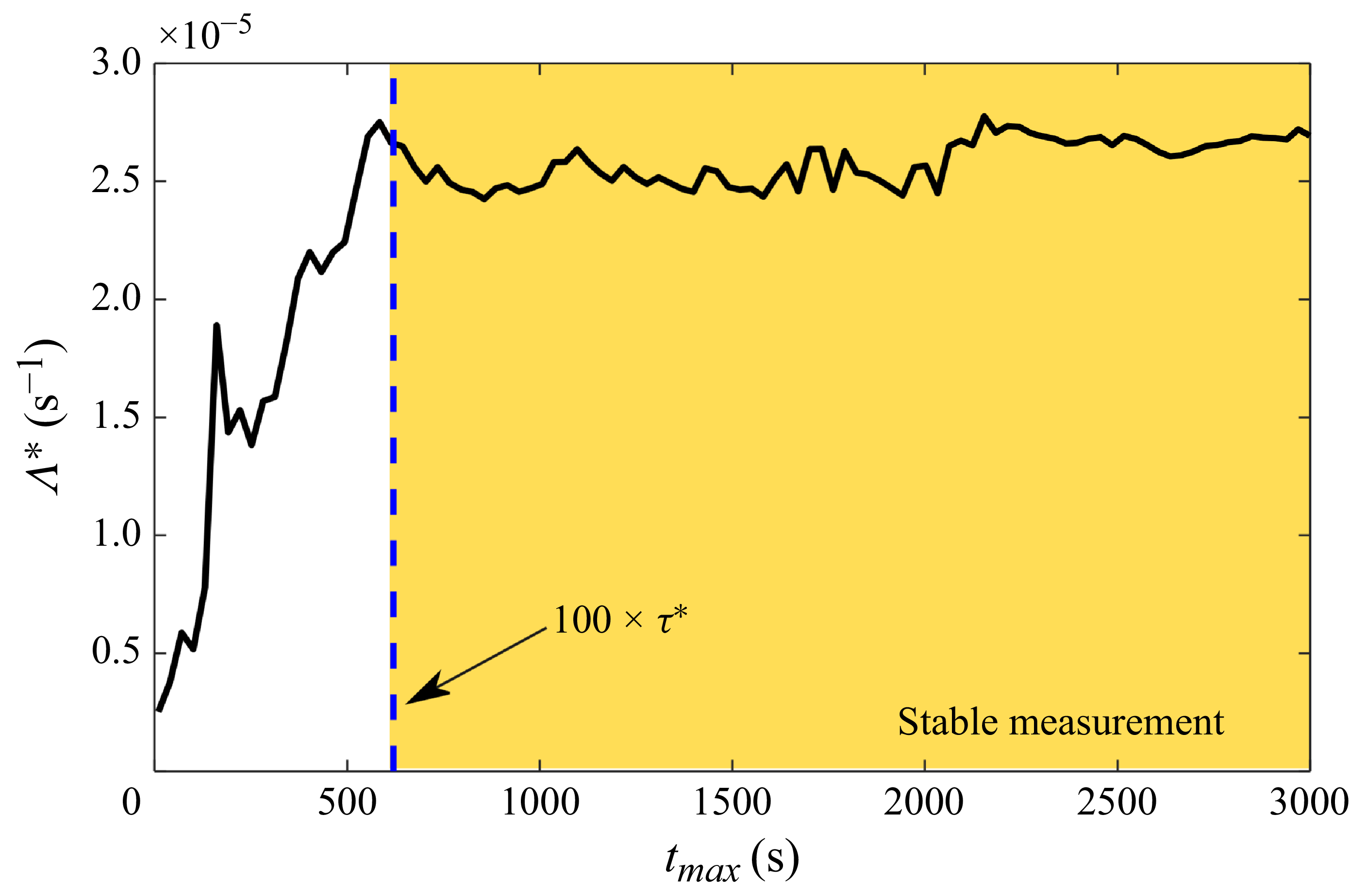


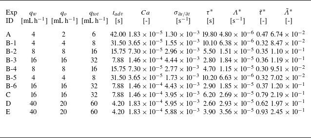


 Open access

