


1. Introduction
Minimising drag in low-Reynolds-number flows by shape selection is a canonical problem in fluid mechanics. Indeed, shape optimisation occurs widely in both natural and industrial applications including swimming, ballistics, biofilm formation, barrier design and drug delivery (Champion, Katare & Mitragotri Reference Champion, Katare and Mitragotri2007; Roper et al. Reference Roper, Pepper, Brenner and Pringle2008; Hinton, Hewitt & Hogg Reference Hinton, Hewitt and Hogg2023; Nijjer et al. Reference Nijjer, Li, Kothari, Henzel, Zhang, Tai, Zhou, Cohen, Zhang and Yan2023; Liu et al. Reference Liu, Zhu, Guo, Bonnet and Veerapaneni2025). In many of these contexts, the ambient fluid can have complicated rheology including shear-thinning or shear-thickening behaviour as well as a yield stress (Hewitt Reference Hewitt2024; Xia et al. Reference Xia, Yu, Lin and Ishikawa2025).
Schematics of a two-dimensional and a three-dimensional optimal body translating at velocity $\mathcal{U}$
. The exterior and interior half-tip angles are denoted by
$\mathcal{U}$
. The exterior and interior half-tip angles are denoted by $\alpha$
and
$\alpha$
and $\beta$
, respectively.
$\beta$
, respectively.

In the context of Stokes flows, Pironneau (Reference Pironneau1973) presented two key results concerning the lowest-drag shape of fixed volume that translates at constant speed: (i) the vorticity is constant over the surface of the body and (ii) the shape at the tips can then be shown to be conical with internal half-angle of $\beta =60^\circ$
. These ideas were used to compute the optimal shape numerically (Bourot Reference Bourot1974); its shape is similar to that of a rugby ball with sharp tips at either end (e.g. Figure 1). The constraint of fixed surface area (rather than fixed volume) was investigated by Montenegro-Johnson & Lauga (Reference Montenegro-Johnson and Lauga2015) who related the surface vorticity to the mean curvature and showed that this optimal body is more slender and has tip half-angle of
$\beta =60^\circ$
. These ideas were used to compute the optimal shape numerically (Bourot Reference Bourot1974); its shape is similar to that of a rugby ball with sharp tips at either end (e.g. Figure 1). The constraint of fixed surface area (rather than fixed volume) was investigated by Montenegro-Johnson & Lauga (Reference Montenegro-Johnson and Lauga2015) who related the surface vorticity to the mean curvature and showed that this optimal body is more slender and has tip half-angle of $\beta \approx 30.8^\circ$
.
$\beta \approx 30.8^\circ$
.
The two-dimensional analogue was studied by Richardson (Reference Richardson1995) who found that the magnitude of the vorticity is also constant on the surface of the body but with a sign change across the axis of symmetry. Despite the Stokes paradox in two-dimensional flow and the associated challenge of mathematically matching the interior viscous flow with an outer region that incorporates inertia, Richardson (Reference Richardson1995) was able to analytically calculate the optimal shape, which has exterior half-angle at the tips, $\alpha \approx 128.7^\circ$
(see figure 1; it is the solution to
$\alpha \approx 128.7^\circ$
(see figure 1; it is the solution to $2 \alpha =\tan 2 \alpha$
). Hinton & Dalwadi (Reference Hinton and Dalwadi2026) showed how the results translate to Stokes flows confined within a channel; in this configuration, the optimal shape does not have exactly constant surface vorticity but the tip angles are identical to those in unbounded flow. Some related shape optimisation problems have been studied in linear elasticity (Zabarankin Reference Zabarankin2013).
$2 \alpha =\tan 2 \alpha$
). Hinton & Dalwadi (Reference Hinton and Dalwadi2026) showed how the results translate to Stokes flows confined within a channel; in this configuration, the optimal shape does not have exactly constant surface vorticity but the tip angles are identical to those in unbounded flow. Some related shape optimisation problems have been studied in linear elasticity (Zabarankin Reference Zabarankin2013).
The purpose of the present paper is to explore the generalisation of these ideas to viscoplastic and power-law fluids. A major challenge here is the nonlinearity introduced by the constitutive law and the presence of regions where the material is rigid. After introducing the mathematical formulation in § 2, we show in § 3 that the optimal body in a Herschel–Bulkley fluid has surface vorticity that is nowhere singular or vanishing. In § 4, the change in the drag on a general body following a small change in shape is calculated for power-law fluids and viscoplastic fluids with relatively large yield stress. The change in the drag is related to the surface vorticity with slightly different forms depending on the rheology of the fluid. It is then straightforward to show that the lowest-drag body of fixed volume (or area if in two dimensions) has constant surface vorticity in any power-law fluid and any viscoplastic fluid at relatively high values of the yield stress.
In § 5, the non-vanishing, non-singular surface vorticity result is used as the basis for a local analysis of the flow at the two sharp tips (see figure 1). This determines the tip angles and their dependency on the rheological parameters. Finally, in § 6, the work is summarised, future directions are suggested and we discuss two additional uses of the variational results from § 4: (i) an alternative method to calculate the drag on a cylinder at high Bingham numbers and (ii) to relate the drag on the optimal body to the value of the constant surface vorticity.
Some ancillary details are included in the four appendices. The altered constraint of fixed surface area is discussed in Appendix A whilst the altered objective of minimising the dissipation potential is analysed in Appendix B, where it is shown that in this case the optimal body has constant surface vorticity for any Herschel–Bulkley fluid. Appendices C and D present the asymptotic structure of the local flow at the tips of the optimal two-dimensional body in the regimes of strong shear-thickening and of high yield stress, respectively.
2. Mathematical formulation
We consider a body with length scale $\mathcal{R}$
that translates at constant velocity
$\mathcal{R}$
that translates at constant velocity $\mathcal{U}$
within an unbounded domain of incompressible Herschel–Bulkley fluid (figure 1). The body may be two- or three-dimensional and the length scale
$\mathcal{U}$
within an unbounded domain of incompressible Herschel–Bulkley fluid (figure 1). The body may be two- or three-dimensional and the length scale $\mathcal{R}$
can be defined based upon the constraint (e.g. fixed volume).
$\mathcal{R}$
can be defined based upon the constraint (e.g. fixed volume).
To make the problem dimensionless, we scale all lengths with $\mathcal{R}$
, velocities with
$\mathcal{R}$
, velocities with $\mathcal{U}$
and pressures and stresses with
$\mathcal{U}$
and pressures and stresses with $K \mathcal{U}^N/\mathcal{R}^N$
, where
$K \mathcal{U}^N/\mathcal{R}^N$
, where $K$
is the consistency of the fluid and
$K$
is the consistency of the fluid and $N\gt 0$
the power-law index. This introduces the Bingham number, which is the ratio of the yield strength of the fluid
$N\gt 0$
the power-law index. This introduces the Bingham number, which is the ratio of the yield strength of the fluid $\tau _Y$
to the characteristic viscous stress in the flow:
$\tau _Y$
to the characteristic viscous stress in the flow:
 \begin{equation} B = \frac {\tau _Y \mathcal{R}^N}{K \mathcal{U}^N}. \end{equation}
In this dimensionless framework, the components of Cauchy’s stress tensor are given by
 \begin{equation} \sigma _{\textit{ij}} = - p \delta _{\textit{ij}} + \tau _{\textit{ij}}, \end{equation}
where $p$
is the pressure and
$p$
is the pressure and $\tau _{\textit{ij}}$
are the components of the deviatoric stress tensor, which are related to the velocity gradients via the Herschel–Bulkley constitutive law:
$\tau _{\textit{ij}}$
are the components of the deviatoric stress tensor, which are related to the velocity gradients via the Herschel–Bulkley constitutive law:
 \begin{equation} \dot {\gamma }_{\textit{ij}}=0 \quad \text{if} \quad \tau \leq B, \end{equation}
or
 \begin{equation} \tau _{\textit{ij}}=\left (\dot {\gamma }^{N-1} +\frac {B}{\dot {\gamma }} \right ) \dot {\gamma }_{\textit{ij}} \quad \text{if} \quad \tau \gt B, \end{equation}
where
 \begin{equation} \dot {\gamma }_{\textit{ij}} = \frac {\partial u_i}{\partial x_{\!j}} + \frac {\partial u_{\!j}}{\partial x_i}, \quad \dot {\gamma } = \sqrt {\frac {1}{2} \sum _{i,j} \dot {\gamma }_{\textit{ij}}\dot {\gamma }_{\textit{ij}}}, \quad \tau = \sqrt {\frac {1}{2} \sum _{i,j} \tau _{\textit{ij}}\tau _{\textit{ij}}}. \end{equation}
The governing equations consist of Cauchy’s momentum equation and mass conservation:
 \begin{equation} \frac {\partial \sigma _{\textit{ij}}}{\partial x_{\!j}} =0 \quad \text{and} \quad \frac {\partial u_{\!j}}{\partial x_{\!j}} =0. \end{equation}
The boundary conditions are unit velocity in the $x_1$
direction,
$x_1$
direction, $u_i = \delta _{1i}$
, on the body boundary,
$u_i = \delta _{1i}$
, on the body boundary, $\partial S$
, and
$\partial S$
, and $u_i \to 0$
in the far field. On the surface of the body, the magnitude of the vorticity is denoted by
$u_i \to 0$
in the far field. On the surface of the body, the magnitude of the vorticity is denoted by $\omega$
, which satisfies
$\omega$
, which satisfies
 \begin{equation} \omega ^2 = \dot {\gamma }^2= \frac {\partial u_i}{\partial n}\frac {\partial u_i}{\partial n}. \end{equation}
In other words, the magnitude of the vorticity on the surface of the body, $\omega$
, is equal to the strain rate there,
$\omega$
, is equal to the strain rate there, $\dot {\gamma }$
. Hence all results concerning the surface vorticity also apply to the surface strain rate (and vice versa). The dimensionless force on the body is given by
$\dot {\gamma }$
. Hence all results concerning the surface vorticity also apply to the surface strain rate (and vice versa). The dimensionless force on the body is given by
 \begin{equation} F_i= \int _{\partial S} \sigma _{\textit{ij}} n_{\!j} \, \mathrm{d} S, \end{equation}
where the normal vector points out of the body into the fluid and has components $n_{\!j}$
. The force in the
$n_{\!j}$
. The force in the $x$
direction,
$x$
direction, $F_1$
, is negative and so the drag is
$F_1$
, is negative and so the drag is $-F_1$
. We are interested in the properties of the lowest-drag body (e.g. the tip angle or the surface vorticity) and how those properties depend on the fluid rheology and the constraint. In the main text of this paper, results are focused on the three-dimensional drag-minimising body with fixed volume and the two-dimensional analogue with fixed area. The constraint of a fixed surface area for a three-dimensional body is discussed in Appendix A.
$-F_1$
. We are interested in the properties of the lowest-drag body (e.g. the tip angle or the surface vorticity) and how those properties depend on the fluid rheology and the constraint. In the main text of this paper, results are focused on the three-dimensional drag-minimising body with fixed volume and the two-dimensional analogue with fixed area. The constraint of a fixed surface area for a three-dimensional body is discussed in Appendix A.
Since the body translates with unit velocity in the $x_1$
direction, the drag may be written as
$x_1$
direction, the drag may be written as
 \begin{equation} -F_1=-\int _{\partial S} u_i\sigma _{\textit{ij}} n_{\!j} \, \mathrm{d}S. \end{equation}
It is also sometimes convenient to rewrite this in terms of the dissipation by applying the divergence theorem:
 \begin{equation} -F_1=\int _V \frac {1}{2}\dot {\gamma }_{\textit{ij}} \tau _{\textit{ij}} \, \mathrm{d}V= \int _V B\dot {\gamma }+\dot {\gamma }^{N+1} \,\mathrm{d}V, \end{equation}
where $V$
is the fluid domain outside the body, which may be two- or three-dimensional.
$V$
is the fluid domain outside the body, which may be two- or three-dimensional.
3. Surface vorticity on the drag-minimising body in a Herschel–Bulkley fluid
In this section, we show that on the surface of the drag-minimising body translating in a Herschel–Bulkley fluid, the vorticity (and the strain rate) cannot vanish or become singular, even at a point where the body surface is not smooth. The expression for the drag (2.10) is used to construct the following cost function:
 \begin{equation} {J =\int _V B\dot {\gamma }+\dot {\gamma }^{N+1} \,\mathrm{d}V +\lambda \left (V_0-\int _{\textit{body}}\,\mathrm{d}V\right )\!,} \end{equation}
where $\lambda$
is a Lagrange multiplier imposing fixed volume (or area if in a planar geometry). The optimal body is an extremum of
$\lambda$
is a Lagrange multiplier imposing fixed volume (or area if in a planar geometry). The optimal body is an extremum of $J$
and so following any small change in shape, the variation in
$J$
and so following any small change in shape, the variation in $J$
must vanish.
$J$
must vanish.
Consider a point on the surface of the optimal body, $\boldsymbol{x}$
, and denote the radial distance from this point by
$\boldsymbol{x}$
, and denote the radial distance from this point by $r$
. Then as
$r$
. Then as $r\to 0$
, the strain rate behaves as
$r\to 0$
, the strain rate behaves as $\dot {\gamma }\sim r^{c}$
for some
$\dot {\gamma }\sim r^{c}$
for some $c$
, which is to be determined. The optimal body is perturbed by extending it in a neighbourhood of the point
$c$
, which is to be determined. The optimal body is perturbed by extending it in a neighbourhood of the point $\boldsymbol{x}$
by a radial distance
$\boldsymbol{x}$
by a radial distance $\varepsilon \ll 1$
(e.g. see figure 2
a). In a three-dimensional geometry, the corresponding change in the drag (2.10) is proportional to
$\varepsilon \ll 1$
(e.g. see figure 2
a). In a three-dimensional geometry, the corresponding change in the drag (2.10) is proportional to $\varepsilon ^{3+c}$
for
$\varepsilon ^{3+c}$
for $c\geq 0$
and to
$c\geq 0$
and to $\varepsilon ^{3+(1+N)c}$
for
$\varepsilon ^{3+(1+N)c}$
for $c\lt 0$
. The change in the volume term in (3.1) is proportional to
$c\lt 0$
. The change in the volume term in (3.1) is proportional to $\varepsilon ^3$
, noting that the Lagrange multiplier,
$\varepsilon ^3$
, noting that the Lagrange multiplier, $\lambda$
, must be independent of the size of the small extension,
$\lambda$
, must be independent of the size of the small extension, $\varepsilon$
. Since the change in
$\varepsilon$
. Since the change in $J$
must vanish, the contribution from the change in the drag term and the volume term must balance, which imposes
$J$
must vanish, the contribution from the change in the drag term and the volume term must balance, which imposes $c=0$
and so, on the optimal body, the strain rate and the vorticity cannot vanish or be singular. The same arguments and conclusion apply to the drag-minimising two-dimensional body of fixed area.
$c=0$
and so, on the optimal body, the strain rate and the vorticity cannot vanish or be singular. The same arguments and conclusion apply to the drag-minimising two-dimensional body of fixed area.


A corollary of this result is that rigid regions (where the strain rate vanishes) are never attached to the drag-minimising body and so fluid is yielded along the entire boundary. Another implication is that at the upstream and downstream points of the optimal body, there must be a sharp tip because a smooth tip would be a stagnation point with vanishing strain rate. In § 5, the tip angles are calculated for different values of the rheological parameters, $N$
and
$N$
and $B$
, by exploiting the fact that the strain rate is non-singular and non-vanishing as the apex is approached.
$B$
, by exploiting the fact that the strain rate is non-singular and non-vanishing as the apex is approached.
4. Perturbation analysis
In this section, a perturbative approach is deployed to show that the vorticity (and strain rate) is constant on the surface of drag-minimising bodies moving in a power-law fluid, or in a Bingham fluid with relatively large yield stress. We first determine the change in the drag on a general body within a power-law fluid following a small variation in the shape (§ 4.1). That result is then used to determine properties of the surface vorticity on the lowest-drag body translating in a power-law fluid (§ 4.2). The arguments are adapted to a Bingham fluid with relatively large yield stress (§§ 4.3 and 4.4).
4.1. Change in body shape within a power-law fluid
For a general (two- or three-dimensional) body moving in a power-law fluid ( $B=0$
), we perturb the body boundary
$B=0$
), we perturb the body boundary $\partial S$
to
$\partial S$
to $\partial \tilde {S}$
via
$\partial \tilde {S}$
via $\boldsymbol{x} \to \boldsymbol{x}+ h^{(\varepsilon )}(\boldsymbol{s}) \boldsymbol{n}$
for some small variation
$\boldsymbol{x} \to \boldsymbol{x}+ h^{(\varepsilon )}(\boldsymbol{s}) \boldsymbol{n}$
for some small variation $h^{(\varepsilon )}(\boldsymbol{s})$
, where
$h^{(\varepsilon )}(\boldsymbol{s})$
, where $\boldsymbol{s}$
parametrises the position on the surface. The velocity field associated with the flow around this perturbed shape is denoted by
$\boldsymbol{s}$
parametrises the position on the surface. The velocity field associated with the flow around this perturbed shape is denoted by $\tilde {\boldsymbol{u}}$
with similar expressions for the pressure, stress and strain rate. The variation in these quantities is denoted by a superscript ‘
$\tilde {\boldsymbol{u}}$
with similar expressions for the pressure, stress and strain rate. The variation in these quantities is denoted by a superscript ‘ ${(\varepsilon )}$
’ e.g.
${(\varepsilon )}$
’ e.g. $\tilde {\boldsymbol{u}}-\boldsymbol{u}=\boldsymbol{u}^{(\varepsilon )}$
.
$\tilde {\boldsymbol{u}}-\boldsymbol{u}=\boldsymbol{u}^{(\varepsilon )}$
.
For a three-dimensional configuration, both velocity fields and the variations of all quantities vanish in the far field. In the two-dimensional case, the boundary conditions are essentially identical but their derivation is a little more subtle owing to the Stokes paradox (for $N\geq 1$
); see Tanner (Reference Tanner1993) and Richardson (Reference Richardson1995).
$N\geq 1$
); see Tanner (Reference Tanner1993) and Richardson (Reference Richardson1995).
The variation to the second tensor invariant of the strain rate (2.5 b) is
 \begin{equation} \dot {\gamma }^{(\varepsilon )}= \frac {1 }{2\dot {\gamma }}\sum _{i,j}\dot {\gamma }_{\textit{ij}} \dot {\gamma }^{(\varepsilon )}_{\textit{ij}}+ o(h^{(\varepsilon )}). \end{equation}
An identical result applies to the second tensor invariant of the stress, $\tau ^{(\varepsilon )}$
. The constitutive law for
$\tau ^{(\varepsilon )}$
. The constitutive law for $B=0$
(2.4) may then be used to obtain the relation
$B=0$
(2.4) may then be used to obtain the relation
 \begin{equation} \sum _{i,j} \dot {\gamma }_{\textit{ij}} \tau ^{(\varepsilon )}_{\textit{ij}} = N \dot {\gamma }^{N-1}\sum _{i,j} \dot {\gamma }_{\textit{ij}}\dot {\gamma }^{(\varepsilon )}_{\textit{ij}}+ o(h^{(\varepsilon )}). \end{equation}
A Taylor expansion of the boundary condition on the perturbed body, $(\boldsymbol{u}+\boldsymbol{u}^{(\varepsilon )})(\boldsymbol{x}+h^{(\varepsilon )}(\boldsymbol{s}) \boldsymbol{n})=\boldsymbol{e}_x$
, gives (Montenegro-Johnson & Lauga Reference Montenegro-Johnson and Lauga2015)
$(\boldsymbol{u}+\boldsymbol{u}^{(\varepsilon )})(\boldsymbol{x}+h^{(\varepsilon )}(\boldsymbol{s}) \boldsymbol{n})=\boldsymbol{e}_x$
, gives (Montenegro-Johnson & Lauga Reference Montenegro-Johnson and Lauga2015)
 \begin{equation} \boldsymbol{u}^{(\varepsilon )}(\boldsymbol{x}) = - h^{(\varepsilon )} \frac {\partial \boldsymbol{u}}{\partial n}. \end{equation}
The drag on the perturbed body may be written as
 \begin{equation} -\tilde {F}_1=-\delta _{i1}\int _{\partial \tilde {S}} \tilde {\sigma }_{\textit{ij}} n_{\!j} \, \mathrm{d}S. \end{equation}
The change in the drag is therefore
 \begin{equation} -F^{(\varepsilon )}_1 = -\delta _{i1} \int _{\partial S} \sigma ^{(\varepsilon )}_{\textit{ij}} n_{\!j} \, \mathrm{d}S- \delta _{i1} \int _{\partial \tilde {S}-\partial S} \sigma _{\textit{ij}} n_{\!j} \, \mathrm{d}S + o(h^{(\varepsilon )}). \end{equation}
Henceforth, we drop the lower-case $o$
notation and include only the leading-order contribution to the drag variation. The second integral in (4.5) vanishes upon applying the divergence theorem (cf. Richardson Reference Richardson1995; Zabarankin Reference Zabarankin2013) and the first may be rewritten as
$o$
notation and include only the leading-order contribution to the drag variation. The second integral in (4.5) vanishes upon applying the divergence theorem (cf. Richardson Reference Richardson1995; Zabarankin Reference Zabarankin2013) and the first may be rewritten as
 \begin{equation} - F^{(\varepsilon )}_1 = -\int _{\partial S} u_i\sigma ^{(\varepsilon )}_{\textit{ij}} n_{\!j} \, \mathrm{d}S = \int _V \frac {\partial }{\partial x_{\!j}} \big (u_i\sigma ^{(\varepsilon )}_{\textit{ij}}\big ) \, \mathrm{d}V. \end{equation}
Using mass continuity and the momentum equation, this becomes
 \begin{equation} -F^{(\varepsilon )}_1 =\frac {1}{2}\int _V \dot {\gamma }_{\textit{ij}} \tau ^{(\varepsilon )}_{\textit{ij}} \, \mathrm{d}V. \end{equation}
We substitute (4.2) for the stress perturbation to obtain
 \begin{equation} -F^{(\varepsilon )}_1 =\frac {1}{2}\int _{V} N \dot {\gamma }^{N-1}\dot {\gamma }_{\textit{ij}}\dot {\gamma }^{(\varepsilon )}_{\textit{ij}} \, \mathrm{d}V. \end{equation}
Integrating by parts gives
 \begin{equation} -F^{(\varepsilon )}_1 =\int _V \frac {\partial }{\partial x_{\!j}}\big ( u^{(\varepsilon )}_i N \dot {\gamma }^{N-1} \dot {\gamma }_{\textit{ij}} \big )- u^{(\varepsilon )}_i\frac {\partial }{\partial x_{\!j}}\big ( N \dot {\gamma }^{N-1} \dot {\gamma }_{\textit{ij}} \big ) \, \mathrm{d}V. \end{equation}
For the second term we use the constitutive law (2.4) and relate the stress to the pressure via momentum conservation, to obtain
 \begin{equation} \int _{V} u^{(\varepsilon )}_i\frac {\partial }{\partial x_{\!j}}\big ( N \dot {\gamma }^{N-1} \dot {\gamma }_{\textit{ij}} \big) \, \mathrm{d}V=\int _{V} \textit{Nu}^{(\varepsilon )}_i \frac {\partial \tau _{\textit{ij}}}{\partial x_{\!j}} \, \mathrm{d}V=\int _{V} \textit{Nu}^{(\varepsilon )}_i \frac {\partial p}{\partial x_i} \, \mathrm{d}V. \end{equation}
Again using mass continuity and the divergence theorem, this can be shown to vanish by applying (4.3):
 \begin{equation} \int _V \textit{Nu}^{(\varepsilon )}_i \frac {\partial p}{\partial x_i} \, \mathrm{d}V = -\int _{\partial S} \textit{Nu}^{(\varepsilon )}_i p n_i\,\mathrm{d}S = \int _{\partial S} \textit{Nh}^{(\varepsilon )} \frac {\partial u_i}{\partial n} p n_i\,\mathrm{d}S =0. \end{equation}
The drag perturbation (4.9) can be written as
 \begin{equation} -F^{(\varepsilon )}_1 =-\int _{\partial S} u^{(\varepsilon )}_i N \dot {\gamma }^{N-1} \dot {\gamma }_{\textit{ij}} n_{\!j}\,\mathrm{d}S=\int _{\partial S} h^{(\varepsilon )} \frac {\partial u_i}{\partial n} N \dot {\gamma }^{N-1} \dot {\gamma }_{\textit{ij}} n_{\!j}\,\mathrm{d}S. \end{equation}
Finally, since $\dot {\gamma }_{\textit{ij}} n_{\!j}= {\partial u_i}/{\partial n}$
on the surface, we obtain
$\dot {\gamma }_{\textit{ij}} n_{\!j}= {\partial u_i}/{\partial n}$
on the surface, we obtain
 \begin{equation} -F^{(\varepsilon )}_1 =N\int _{\partial S} h^{(\varepsilon )} \dot {\gamma }^{N+1} \,\mathrm{d}S, \end{equation}
which holds for any power-law fluid in both two-dimensional and three-dimensional geometries. The result (4.13) relates the change in drag following a small change in shape (for any body) to the magnitude of the vorticity (i.e. the strain rate) on the surface. It reduces to the Newtonian result of Pironneau (Reference Pironneau1973) and Richardson (Reference Richardson1995) when $N=1$
. In § 4.2, (4.13) is used to determine the surface vorticity on drag-minimising bodies but it also has additional uses, as discussed in § 6.
$N=1$
. In § 4.2, (4.13) is used to determine the surface vorticity on drag-minimising bodies but it also has additional uses, as discussed in § 6.
4.2. Surface vorticity on the optimal body in power-law fluids
We now consider the implications of (4.13) for the lowest-drag body under the constraints of fixed volume (three-dimensional) and fixed area (two-dimensional). The case of fixed surface area (three-dimensional) is discussed in Appendix A.
For a three-dimensional body of fixed volume, $V_0$
, we consider the cost function,
$V_0$
, we consider the cost function, $J$
, from (3.1). Leading-order variations in this cost function are given by
$J$
, from (3.1). Leading-order variations in this cost function are given by
 \begin{equation} J^{(\varepsilon )} =\int _{\partial S} h^{(\varepsilon )}\big ( N \dot {\gamma }^{N+1}-\lambda \big ) \,\mathrm{d}S. \end{equation}
The lowest-drag body satisfies $J^{(\varepsilon )} =0$
and since
$J^{(\varepsilon )} =0$
and since $\dot {\gamma }$
is positive and
$\dot {\gamma }$
is positive and $\lambda$
is a constant, we find that on the surface of this body, the strain rate (and hence the vorticity) is constant. The stress is also constant. The same result applies to the optimal two-dimensional body of fixed area.
$\lambda$
is a constant, we find that on the surface of this body, the strain rate (and hence the vorticity) is constant. The stress is also constant. The same result applies to the optimal two-dimensional body of fixed area.
4.3. Change in body shape within a high-Bingham-number fluid
In this subsection, we determine the change in the drag on a general body within a high-Bingham-number fluid ( $B\gg 1$
) following a small change in shape
$B\gg 1$
) following a small change in shape $h^{(\varepsilon )}(\boldsymbol{s})$
(for clarity of the analysis, we restrict attention to a Bingham fluid,
$h^{(\varepsilon )}(\boldsymbol{s})$
(for clarity of the analysis, we restrict attention to a Bingham fluid, $N=1$
). The result can then be used to show that the surface vorticity on the lowest-drag body in a high-Bingham-number fluid is constant (§ 4.4).
$N=1$
). The result can then be used to show that the surface vorticity on the lowest-drag body in a high-Bingham-number fluid is constant (§ 4.4).
In the high- $B$
regime, the flow domain mostly consists of regions that are unyielded or weakly yielded (approximately perfect plastic flow) with the remaining material forming thin ‘viscoplastic boundary layers’, where the shear rate is much larger (Piau Reference Piau2002; Balmforth et al. Reference Balmforth, Craster, Hewitt, Hormozi and Maleki2017; Taylor-West Reference Taylor-West2023). These boundary layers fall into two types: those that separate the body boundary from the bulk flow and those that separate two regions of unyielded (or perfectly plastic) material.
$B$
regime, the flow domain mostly consists of regions that are unyielded or weakly yielded (approximately perfect plastic flow) with the remaining material forming thin ‘viscoplastic boundary layers’, where the shear rate is much larger (Piau Reference Piau2002; Balmforth et al. Reference Balmforth, Craster, Hewitt, Hormozi and Maleki2017; Taylor-West Reference Taylor-West2023). These boundary layers fall into two types: those that separate the body boundary from the bulk flow and those that separate two regions of unyielded (or perfectly plastic) material.
In § 4.1, (4.7) was derived for the drag variation following a shape change without reference to the constitutive law and so it applies to a Bingham fluid at high $B$
. Any region of plastic flow can be approximated by power-law fluid with
$B$
. Any region of plastic flow can be approximated by power-law fluid with $N \to 0$
and so the contribution to the drag perturbation from these regions vanishes; see (4.8). The contribution to the drag perturbation from any rigid region also vanishes and so, for high Bingham numbers, the only remaining (non-negligible) contributions to the drag perturbation come from the two types of viscoplastic boundary layers.
$N \to 0$
and so the contribution to the drag perturbation from these regions vanishes; see (4.8). The contribution to the drag perturbation from any rigid region also vanishes and so, for high Bingham numbers, the only remaining (non-negligible) contributions to the drag perturbation come from the two types of viscoplastic boundary layers.
Within the boundary layers, we move to a coordinate system $(s,n)$
, which is defined along and perpendicular to the boundary layer, respectively (both for a two-dimensional geometry and a three-dimensional axisymmetric geometry), and the corresponding velocity components are denoted by
$(s,n)$
, which is defined along and perpendicular to the boundary layer, respectively (both for a two-dimensional geometry and a three-dimensional axisymmetric geometry), and the corresponding velocity components are denoted by $(u,v)$
. The flow in the boundary layers is approximately unidirectional in the
$(u,v)$
. The flow in the boundary layers is approximately unidirectional in the $s$
direction and the dominant contributions to the strain rate and the stress at high
$s$
direction and the dominant contributions to the strain rate and the stress at high $B$
are given by (Balmforth et al. Reference Balmforth, Craster, Hewitt, Hormozi and Maleki2017; Taylor-West Reference Taylor-West2023)
$B$
are given by (Balmforth et al. Reference Balmforth, Craster, Hewitt, Hormozi and Maleki2017; Taylor-West Reference Taylor-West2023)
 \begin{equation} \dot {\gamma } = |\dot {\gamma }_{\textit{sn}}|=\left \lvert \frac {\partial u}{\partial n} \right \rvert , \quad \tau = |\tau _{\textit{sn}}|, \quad \tau _{\textit{sn}} =\dot {\gamma }_{\textit{sn}}\pm B, \end{equation}
where the sign depends on the direction of the shear. Following a small change in shape, the dominant perturbed quantities satisfy
 \begin{equation} \tau _{\textit{sn}}^{(\varepsilon )} = \dot {\gamma }_{\textit{sn}}^{(\varepsilon )}=\frac {\partial u^{(\varepsilon )}}{\partial n}. \end{equation}
The leading-order contributions to the drag perturbation (4.7) at high $B$
can then be written as
$B$
can then be written as
 \begin{equation} {-F^{(\varepsilon )}_1 =\frac {1}{2}\int _{V_{\textit{BL}}} \frac {\partial u}{\partial n}\frac {\partial u^{(\varepsilon )}}{\partial n} \, \mathrm{d}V,} \end{equation}
where $V_{\textit{BL}}$
denotes the viscoplastic boundary-layer regions. Boundary layers that are adjacent to the body have thicknesses of order
$V_{\textit{BL}}$
denotes the viscoplastic boundary-layer regions. Boundary layers that are adjacent to the body have thicknesses of order $B^{-1/2}$
and also the strain rate there is of order
$B^{-1/2}$
and also the strain rate there is of order $B^{1/2}$
(Balmforth et al. Reference Balmforth, Craster, Hewitt, Hormozi and Maleki2017; Supekar, Hewitt & Balmforth Reference Supekar, Hewitt and Balmforth2020; Taylor-West Reference Taylor-West2023). In addition,
$B^{1/2}$
(Balmforth et al. Reference Balmforth, Craster, Hewitt, Hormozi and Maleki2017; Supekar, Hewitt & Balmforth Reference Supekar, Hewitt and Balmforth2020; Taylor-West Reference Taylor-West2023). In addition, $\partial u^{(\varepsilon )}/\partial n$
is of order
$\partial u^{(\varepsilon )}/\partial n$
is of order $h^{(\varepsilon )} B$
owing to the boundary condition on the body, (4.3). In contrast, the boundary layers that do not contact the body have thickness of order
$h^{(\varepsilon )} B$
owing to the boundary condition on the body, (4.3). In contrast, the boundary layers that do not contact the body have thickness of order $B^{-1/3}$
, the strain rate there is of order
$B^{-1/3}$
, the strain rate there is of order $B^{1/3}$
and
$B^{1/3}$
and $\partial u^{(\varepsilon )}/\partial n$
is of order
$\partial u^{(\varepsilon )}/\partial n$
is of order $h^{(\varepsilon )} B^{1/3}$
. Thus body-adjacent boundary layers give a contribution of order
$h^{(\varepsilon )} B^{1/3}$
. Thus body-adjacent boundary layers give a contribution of order $B h^{(\varepsilon )}$
to the drag perturbation (4.17), whilst the other boundary layers give a contribution of order
$B h^{(\varepsilon )}$
to the drag perturbation (4.17), whilst the other boundary layers give a contribution of order $h^{(\varepsilon )} B^{1/3}$
.
$h^{(\varepsilon )} B^{1/3}$
.
In the high-Bingham-number regime, the drag on a general body is proportional to $B$
(Chaparian & Frigaard Reference Chaparian and Frigaard2017b
; Supekar et al. Reference Supekar, Hewitt and Balmforth2020) and so the variation in the drag following a change in shape of size
$B$
(Chaparian & Frigaard Reference Chaparian and Frigaard2017b
; Supekar et al. Reference Supekar, Hewitt and Balmforth2020) and so the variation in the drag following a change in shape of size $h^{(\varepsilon )}$
is proportional to
$h^{(\varepsilon )}$
is proportional to $\textit{Bh}^{(\varepsilon )}$
. Hence, there must be a viscoplastic boundary layer adjacent to some part of the body boundary and this dominates (4.17). Within this boundary layer, the leading-order governing equations reduce to
$\textit{Bh}^{(\varepsilon )}$
. Hence, there must be a viscoplastic boundary layer adjacent to some part of the body boundary and this dominates (4.17). Within this boundary layer, the leading-order governing equations reduce to
 \begin{equation} \frac {\partial P}{\partial s}= \frac {\partial ^2 u}{\partial n^2}, \quad \frac {\partial P}{\partial n}=0, \end{equation}
where $P$
is a modified pressure that includes geometrical terms of order
$P$
is a modified pressure that includes geometrical terms of order $B$
arising from the momentum balance in curvilinear coordinates following the boundary layer (Hewitt & Balmforth Reference Hewitt and Balmforth2018). The drag perturbation (4.17) is rewritten as
$B$
arising from the momentum balance in curvilinear coordinates following the boundary layer (Hewitt & Balmforth Reference Hewitt and Balmforth2018). The drag perturbation (4.17) is rewritten as
 \begin{equation} -F^{(\varepsilon )}_1 =\frac {1}{2}\int _{V_{\textit{BL}}} \frac {\partial }{\partial n}\left (u^{(\varepsilon )}\frac {\partial u}{\partial n} \right ) - u^{(\varepsilon )}\frac {\partial P}{\partial s}- v^{(\varepsilon )}\frac {\partial P}{\partial n}\, \mathrm{d}V, \end{equation}
where the last term is negligible but has been added for convenience. Using the divergence theorem, the second and third terms become an integral of $P\boldsymbol{u}^{(\varepsilon )}\boldsymbol{\cdot }\boldsymbol{n}$
around the edges of the viscoplastic boundary layer. On the body surface, this term vanishes (see (4.11)) whilst on the other edges of the boundary layer it is
$P\boldsymbol{u}^{(\varepsilon )}\boldsymbol{\cdot }\boldsymbol{n}$
around the edges of the viscoplastic boundary layer. On the body surface, this term vanishes (see (4.11)) whilst on the other edges of the boundary layer it is $o(B)$
and can be neglected. The dominant contribution in (4.19) is then
$o(B)$
and can be neglected. The dominant contribution in (4.19) is then
 \begin{equation} -F^{(\varepsilon )}_1 =-\frac {1}{2}\int _{\partial S_{\textit{BL}}} u^{(\varepsilon )}\frac {\partial u}{\partial n} \, \mathrm{d}S=\frac {1}{2}\int _{\partial S_{\textit{BL}}} h^{(\varepsilon )}\frac {\partial u}{\partial n}\frac {\partial u}{\partial n} \, \mathrm{d}S, \end{equation}
where $\partial S_{\textit{BL}}$
denotes the part of the body boundary adjacent to a viscoplastic boundary layer. The expression (4.20) represents the change in drag on a general body (no assumptions about the optimality of the body have been made to obtain (4.20)). Indeed, in § 6, (4.20) is deployed to provide an alternative method for calculating the drag on a cylinder in the high-Bingham-number limit. The result agrees with the literature, which provides a useful check on the validity of (4.20).
$\partial S_{\textit{BL}}$
denotes the part of the body boundary adjacent to a viscoplastic boundary layer. The expression (4.20) represents the change in drag on a general body (no assumptions about the optimality of the body have been made to obtain (4.20)). Indeed, in § 6, (4.20) is deployed to provide an alternative method for calculating the drag on a cylinder in the high-Bingham-number limit. The result agrees with the literature, which provides a useful check on the validity of (4.20).
4.4. Surface vorticity on the optimal body in high-Bingham-number fluids
Equation (4.20) indicates that in any part of the body boundary where the material is rigid (or perfectly plastic), the shape can be increased in size along the normal direction without increasing the drag. This body is not optimal. Hence there cannot be any part of the boundary of the optimal body that is not in contact with a viscoplastic boundary layer, i.e. $\partial S_{\textit{BL}}= \partial S$
. The change in drag on the optimal body is then given by
$\partial S_{\textit{BL}}= \partial S$
. The change in drag on the optimal body is then given by
 \begin{equation} -F^{(\varepsilon )}_1 =\frac {1}{2}\int _{\partial S} h^{(\varepsilon )}\frac {\partial u}{\partial n}\frac {\partial u}{\partial n} \, \mathrm{d}S, \end{equation}
which is identical to the result for a Newtonian fluid (4.13), except for the factor of $1/2$
. Setting the variation in the cost function
$1/2$
. Setting the variation in the cost function $J$
(3.1) to zero furnishes the result that the lowest-drag body of fixed area or volume in a Bingham fluid with
$J$
(3.1) to zero furnishes the result that the lowest-drag body of fixed area or volume in a Bingham fluid with $B\gg 1$
has constant surface vorticity (and surface strain rate).
$B\gg 1$
has constant surface vorticity (and surface strain rate).
For a Herschel–Bulkley fluid more generally, the surface vorticity on the drag-minimising body is not necessarily constant (although it cannot vanish or be singular; see § 3). However, if we instead consider bodies that minimise a slightly different functional – the dissipation potential – then the constant-surface-vorticity result applies to any Herschel–Bulkley fluid (see Appendix B).
5. Local analysis at the ends of the optimal body
In this section, the condition of constant surface vorticity as the optimal body’s tip is approached (§ 3) is used to perform a local analysis of the flow at the two ends of the body. As well as providing insight to the flow physics in these regions, the analysis also furnishes the tip angle of the optimal body over a wide range of $B$
and
$B$
and $N$
. The optimal body is symmetric about both axes and we denote the interior half-tip angle by
$N$
. The optimal body is symmetric about both axes and we denote the interior half-tip angle by $\beta$
and the exterior half-tip angle by
$\beta$
and the exterior half-tip angle by $\alpha =\pi -\beta$
(see figure 1). Two-dimensional optimal bodies are analysed in § 5.1 and the three-dimensional analogue is analysed in § 5.2. In all cases, the local region under investigation is taken to be smaller than any important flow regions about the body and in particular, for high Bingham numbers, the local region is entirely contained within the viscoplastic boundary layer (see figure 2
b).
$\alpha =\pi -\beta$
(see figure 1). Two-dimensional optimal bodies are analysed in § 5.1 and the three-dimensional analogue is analysed in § 5.2. In all cases, the local region under investigation is taken to be smaller than any important flow regions about the body and in particular, for high Bingham numbers, the local region is entirely contained within the viscoplastic boundary layer (see figure 2
b).
5.1. Two-dimensional optimal body of fixed area
To investigate the flow in the vicinity of the tips, we use polar coordinates centred at the apex, $(a,0)$
:
$(a,0)$
:
 \begin{equation} (x,y) = (a,0) + r (\cos \theta , \sin \theta ). \end{equation}
The behaviour at the other apex is then obtained via symmetry. The radial velocity is denoted by $u$
and the azimuthal velocity by
$u$
and the azimuthal velocity by $v$
. The governing equations are
$v$
. The governing equations are
 \begin{align} \frac {1}{r}&\frac {\partial }{\partial r}(\textit{ru}) + \frac {1}{r}\frac {\partial v}{\partial \theta } = 0, \\[-12pt]\nonumber \end{align}
 \begin{align} \frac {\partial p}{\partial r} &= \frac {\partial \tau _{rr}}{\partial r} + \frac {1}{r}\frac {\partial \tau _{r\theta }}{\partial \theta } + \frac {2}{r}\tau _{rr}, \\[-12pt]\nonumber \end{align}
 \begin{align} \frac {1}{r}\frac {\partial p}{\partial \theta } &= \frac {\partial \tau _{r\theta }}{\partial r} - \frac {1}{r}\frac {\partial \tau _{rr}}{\partial \theta } + \frac {2}{r}\tau _{r\theta }. \end{align}
Near the apex, the flow is yielded and so the constitutive law takes the form
 \begin{equation} (\tau _{rr},\tau _{r\theta }) = \left (\dot {\gamma }^{N-1}+\frac {B}{\dot {\gamma }} \right ) (\dot {\gamma }_{rr},\dot {\gamma }_{r\theta }), \end{equation}
with
 \begin{equation} \dot {\gamma }_{rr} = 2 \frac {\partial u}{\partial r}, \quad \dot {\gamma }_{r\theta }=\frac {1}{r} \frac {\partial u}{\partial \theta } + \frac {\partial v}{\partial r} - \frac {v}{r} \end{equation}
and
 \begin{equation} \dot {\gamma } = \sqrt { \left (\frac {1}{r} \frac {\partial u}{\partial \theta } + \frac {\partial v}{\partial r} - \frac {v}{r}\right )^2+4 \left (\frac {\partial u}{\partial r} \right )^2}. \end{equation}
The optimality condition from § 3 imposes non-singular and non-vanishing vorticity as the apex is approached ( $r \to 0$
), which imposes the following form for the velocities:
$r \to 0$
), which imposes the following form for the velocities:
 \begin{equation} (u,v) =(\cos \theta ,-\sin \theta )+ r \left (f'(\theta ),-2f(\theta ) \right )\!, \end{equation}
for some function $f(\theta )$
, where we have also used mass continuity, and the first term in (5.8) accounts for the translation of the body. The strain rates then take the forms
$f(\theta )$
, where we have also used mass continuity, and the first term in (5.8) accounts for the translation of the body. The strain rates then take the forms
 \begin{equation} \dot {\gamma }_{rr} = 2 f'(\theta ), \quad \dot {\gamma }_{r\theta }=f''(\theta ), \quad \dot {\gamma } = \sqrt {f''(\theta )^2+4f'(\theta )^2}. \end{equation}
Since the components of the stress tensor are independent of the radial coordinate, its second tensor invariant may be written as
 \begin{equation} \tau = \big (f''(\theta )^2 +4f'(\theta )^2 \big )^{N/2} +B. \end{equation}
Using (5.4), the pressure may be written as (Alexandrov & Jeng Reference Alexandrov and Jeng2009; Taylor-West & Hogg Reference Taylor-West and Hogg2023)
 \begin{equation} p = 2 \chi B \log r + m(\theta ), \end{equation}
for some constant $\chi$
and a function of integration
$\chi$
and a function of integration $m(\theta )$
. The radial momentum equation (5.3) becomes an ordinary differential equation for
$m(\theta )$
. The radial momentum equation (5.3) becomes an ordinary differential equation for $f(\theta )$
:
$f(\theta )$
:
 \begin{align} \begin{split} 2 \chi B =& \frac {\mathrm{d}}{\mathrm{d} \theta } \left [ \left (\big(f^{\prime \prime 2} +4f^{\prime 2} \big)^{(N-1)/2}f''+\frac {B}{\left (f^{\prime \prime 2} +4f^{\prime 2} \right )^{1/2}}\right )\right ]\\ &+4 \left (\big (f^{\prime \prime 2} +4f^{\prime 2} \big )^{(N-1)/2} +\frac {B}{\left (f^{\prime \prime 2} +4f^{\prime 2} \right )^{1/2}}\right )f'. \end{split} \end{align}
For $N=1$
, this can be reduced to equation (A1) of Taylor-West & Hogg (Reference Taylor-West and Hogg2023).
$N=1$
, this can be reduced to equation (A1) of Taylor-West & Hogg (Reference Taylor-West and Hogg2023).
It was shown in § 3 that in any Herschel–Bulkley fluid $\dot {\gamma }\sim r^0$
as
$\dot {\gamma }\sim r^0$
as $r\to 0$
and so in the region local to the tip, the surface strain rate (and surface vorticity) are constant. The boundary conditions on the wall of the body, at
$r\to 0$
and so in the region local to the tip, the surface strain rate (and surface vorticity) are constant. The boundary conditions on the wall of the body, at $\theta =\alpha$
, are then given by no-slip and no-flux as well as constant magnitude of the surface vorticity denoted by
$\theta =\alpha$
, are then given by no-slip and no-flux as well as constant magnitude of the surface vorticity denoted by $\omega$
. Two additional boundary conditions are given by symmetry at
$\omega$
. Two additional boundary conditions are given by symmetry at $\theta =0$
, furnishing
$\theta =0$
, furnishing
 \begin{equation} f(\alpha )=f'(\alpha )=0, \quad f''(\alpha )^2=\omega ^2, \quad f(0)=f''(0)=0. \end{equation}
The magnitude of the surface vorticity (i.e. the surface strain rate) $\omega$
in this local region is in general an unknown constant that depends on the rheological parameters
$\omega$
in this local region is in general an unknown constant that depends on the rheological parameters $B$
and
$B$
and $N$
. To determine
$N$
. To determine $\omega$
would require full numerical simulations that incorporate the outer flow (although some analytical progress is possible in special cases such as high
$\omega$
would require full numerical simulations that incorporate the outer flow (although some analytical progress is possible in special cases such as high $B$
; see § 6).
$B$
; see § 6).
The governing equation (5.12) is a third-order ordinary differential equation for $f(\theta )$
with five boundary conditions and three unknowns:
$f(\theta )$
with five boundary conditions and three unknowns: $\alpha$
,
$\alpha$
, $\omega$
,
$\omega$
, $\chi$
. In general, the system cannot be solved without knowing the surface vorticity,
$\chi$
. In general, the system cannot be solved without knowing the surface vorticity, $\omega$
, in advance. However, progress can be made either in cases where
$\omega$
, in advance. However, progress can be made either in cases where $\omega$
can be scaled out of the problem (e.g. for power-law fluids; § 5.1.1) or by absorbing the surface vorticity into the Bingham number to find solutions that depend on a modified Bingham number (§ 5.1.2).
$\omega$
can be scaled out of the problem (e.g. for power-law fluids; § 5.1.1) or by absorbing the surface vorticity into the Bingham number to find solutions that depend on a modified Bingham number (§ 5.1.2).
5.1.1. Power-law fluid ( $B=0$
)
$B=0$
)

For a power-law fluid with $N\gt 0$
, we rescale the independent coordinate with
$N\gt 0$
, we rescale the independent coordinate with $\alpha$
, defining
$\alpha$
, defining $\theta =\alpha t$
. The eigenvalue
$\theta =\alpha t$
. The eigenvalue $\chi$
is rewritten as
$\chi$
is rewritten as $\chi =A B^{-1}$
and the dependent variable as
$\chi =A B^{-1}$
and the dependent variable as
 \begin{equation} g(t) = (2A)^{-1/N} \alpha ^{-2-\frac {1}{N}} \frac {\mathrm{d} f}{\mathrm{d} t}, \end{equation}
to recast the governing equation (5.12) as
 \begin{equation} 1= \big (g_{tt}+4 \alpha ^2 g\big )\big (g_t^2+4 \alpha ^2 g^2 \big )^{\frac {N-1}{2}} \left ( 1+ \frac {(N-1)g_t^2}{g_t^2 + 4 \alpha ^2 g^2} \right )\!. \end{equation}
The following three boundary conditions:
 \begin{equation} g_t(0)=0, \quad g(1)=0, \quad \int _0^1 g\, \mathrm{d}t=0, \end{equation}
are sufficient to solve the second-order ordinary differential equation (5.15) for $g(t)$
and to obtain the unknown angle
$g(t)$
and to obtain the unknown angle $\alpha$
. The solution,
$\alpha$
. The solution, $g(t)$
, is obtained only up to a multiplicative constant (which is associated with the unknown surface vorticity). The strain rate and the stress are also defined up to a multiplicative constant and given by
$g(t)$
, is obtained only up to a multiplicative constant (which is associated with the unknown surface vorticity). The strain rate and the stress are also defined up to a multiplicative constant and given by
 \begin{equation} \dot {\gamma }\propto \sqrt {g_t g_t+4 \alpha ^2 g^2}, \quad \tau \propto \big (g_t g_t+4 \alpha ^2 g^2\big )^{\tfrac{N}{2}}. \end{equation}
For a Newtonian fluid, the solution is
 \begin{equation} g(t)= \frac {1}{4 \alpha _0^2} \left (1 - \frac {\cos 2 \alpha _0 t}{\cos 2 \alpha _0} \right )\!, \end{equation}
and the integral condition on $g$
furnishes the angle at the tip (Richardson Reference Richardson1995):
$g$
furnishes the angle at the tip (Richardson Reference Richardson1995):
 \begin{equation} 2 \alpha _0 = \tan 2 \alpha _0, \quad \text{so} \quad \alpha _0=128.7^\circ , \quad \beta _0 = 51.3^\circ . \end{equation}
The strain rate (and the stress) for this case are proportional to
 \begin{equation} \dot {\gamma },\tau \propto \sqrt {1+\left (\cos 2\alpha -2\cos 2 \alpha t\right ) \cos 2 \alpha }. \end{equation}
For general $N$
, (5.15) must be solved via numerical integration. We shoot from
$N$
, (5.15) must be solved via numerical integration. We shoot from $t=0$
using the boundary condition
$t=0$
using the boundary condition $g_t(0)=0$
and iterating over different choices of
$g_t(0)=0$
and iterating over different choices of $g(0)$
and
$g(0)$
and $\alpha$
until both remaining conditions in (5.16) are satisfied. The tip angle for different values of
$\alpha$
until both remaining conditions in (5.16) are satisfied. The tip angle for different values of $N$
is shown in figure 3(a).
$N$
is shown in figure 3(a).
(a) Tip angle of the lowest-drag two-dimensional body of fixed area in a power-law fluid of index $N$
. The interior half-angle,
$N$
. The interior half-angle, $\beta$
(
$\beta$
( $=\pi -\alpha$
) is shown in degrees (see also figure 1). The red plus indicates the Newtonian result and the red dashed line is the plastic limit (
$=\pi -\alpha$
) is shown in degrees (see also figure 1). The red plus indicates the Newtonian result and the red dashed line is the plastic limit ( $\beta \to 45^\circ$
as
$\beta \to 45^\circ$
as $N\to 0$
), which is analysed in § 5.1.2, whilst the magenta dotted line is the strongly shear-thickening limit (
$N\to 0$
), which is analysed in § 5.1.2, whilst the magenta dotted line is the strongly shear-thickening limit ( $\beta \to 75^\circ$
as
$\beta \to 75^\circ$
as $N\to \infty$
) (see Appendix C). (b) The strain rate (relative to the surface vorticity)
$N\to \infty$
) (see Appendix C). (b) The strain rate (relative to the surface vorticity) $\dot {\gamma }/\omega$
around the tip. Curves are shown for eight values of the power-law index:
$\dot {\gamma }/\omega$
around the tip. Curves are shown for eight values of the power-law index: $N=2^{\{-2,-1,0,1,2,3,4,5\}}$
. The black line shows the Newtonian case.
$N=2^{\{-2,-1,0,1,2,3,4,5\}}$
. The black line shows the Newtonian case.

The strain rate (relative to the surface vorticity) $\dot {\gamma }/\omega$
around the tip of the lowest-drag two-dimensional body with fixed area in a power-law fluid. Power-law index: (a)
$\dot {\gamma }/\omega$
around the tip of the lowest-drag two-dimensional body with fixed area in a power-law fluid. Power-law index: (a) $N=0.25$
, (b)
$N=0.25$
, (b) $N=1$
, (c)
$N=1$
, (c) $N=32$
. The thick black line indicates the body boundary and yellow lines indicate the streamlines (in the frame moving with the body).
$N=32$
. The thick black line indicates the body boundary and yellow lines indicate the streamlines (in the frame moving with the body).

Further insight can be obtained from figures 3(b) and 4, which show the strain rates (relative to the surface vorticity) in the vicinity of the apex for a range of values of $N$
as well as some of the streamlines in the frame of the moving body. Within a shear-thinning fluid (
$N$
as well as some of the streamlines in the frame of the moving body. Within a shear-thinning fluid ( $N\lt 1$
), the optimal body has sharper tips with the interior half-angle converging to
$N\lt 1$
), the optimal body has sharper tips with the interior half-angle converging to $45^\circ$
in the plastic limit (
$45^\circ$
in the plastic limit ( $N\to 0$
), which is discussed in more detail in § 5.1.2.
$N\to 0$
), which is discussed in more detail in § 5.1.2.
In a shear-thickening fluid, the body has a blunter tip and the interior half-angle converges to $75^\circ$
in the limit
$75^\circ$
in the limit $N\to \infty$
(see Appendix C). The expression for the drag (2.10) indicates that at higher values of
$N\to \infty$
(see Appendix C). The expression for the drag (2.10) indicates that at higher values of $N$
(more shear-thickening), the optimal body must be shaped to minimise regions of high shear more than at lower values of
$N$
(more shear-thickening), the optimal body must be shaped to minimise regions of high shear more than at lower values of $N$
, which leads to a more uniform strain rate. Indeed, for
$N$
, which leads to a more uniform strain rate. Indeed, for $N\gg 1$
, the shape optimisation becomes a minimax problem where the maximum strain rate must be minimised over the fluid domain and so the strain rate is mostly uniform aside from thin bands of low viscosity. One example of these bands can be seen in the
$N\gg 1$
, the shape optimisation becomes a minimax problem where the maximum strain rate must be minimised over the fluid domain and so the strain rate is mostly uniform aside from thin bands of low viscosity. One example of these bands can be seen in the $N=32$
case in figures 3(b) and 4(c). In this case, although the strain rate is only about 10 % lower in the band than the bulk strain rate, the viscosity is about 97 % lower than in the bulk regions owing to the strong shear-thickening nature of the fluid. In the limit as
$N=32$
case in figures 3(b) and 4(c). In this case, although the strain rate is only about 10 % lower in the band than the bulk strain rate, the viscosity is about 97 % lower than in the bulk regions owing to the strong shear-thickening nature of the fluid. In the limit as $N\to \infty$
, the band occurs at
$N\to \infty$
, the band occurs at $\theta =5\pi /12$
(see Appendix C).
$\theta =5\pi /12$
(see Appendix C).
5.1.2. Bingham fluid
For a Bingham fluid ( $N=1$
), (5.12) cannot be solved for general
$N=1$
), (5.12) cannot be solved for general $B\gt 0$
without knowing the surface vorticity,
$B\gt 0$
without knowing the surface vorticity, $\omega$
, in advance. However, the system can be re-framed in terms of a modified Bingham number by writing
$\omega$
, in advance. However, the system can be re-framed in terms of a modified Bingham number by writing
 \begin{equation} f= \omega \hat {f},\quad B=\omega \hat {B}, \quad \theta = \alpha t. \end{equation}
The governing equation (5.12) becomes
 \begin{equation} 2 \chi \hat {B} \alpha ^3= \big (\hat {f}_{ttt}+4 \alpha ^2\hat {f}_t\big) \left (1+\frac {4 \alpha ^4\hat {B}\hat {f}_t^2}{\left (\hat {f}_{tt}^2 +4\alpha ^2\hat {f}_t^2 \right )^{3/2}}\right )\!. \end{equation}
The boundary conditions (5.13) become
 \begin{equation} \hat {f}(1)=\hat {f}_t(1)=0, \quad \hat {f}_{tt}(1)^2=1, \quad \hat {f}(0)=\hat {f}_{tt}(0)=0. \end{equation}
The third-order differential equation (5.22) has five boundary conditions with two unknown constants ( $\alpha$
and
$\alpha$
and $\chi$
), which enables complete solution. The main drawback is that the single parameter
$\chi$
), which enables complete solution. The main drawback is that the single parameter $\hat {B}=B/\omega$
that appears in the governing equation depends on both
$\hat {B}=B/\omega$
that appears in the governing equation depends on both $B$
and
$B$
and $\omega$
, which is itself a function of
$\omega$
, which is itself a function of $B$
. Nonetheless, it is still informative to determine the angle
$B$
. Nonetheless, it is still informative to determine the angle $\alpha$
as well as the solution structure in terms of
$\alpha$
as well as the solution structure in terms of $\hat {B}$
. In addition, a particular regime of interest,
$\hat {B}$
. In addition, a particular regime of interest, $\hat {B}\gg 1$
, corresponds to
$\hat {B}\gg 1$
, corresponds to $B \gg 1$
since
$B \gg 1$
since $\omega \sim B^{1/2}$
in this limit (Balmforth et al. Reference Balmforth, Craster, Hewitt, Hormozi and Maleki2017). The system (5.22) with boundary conditions (5.23) is solved via shooting numerically to obtain
$\omega \sim B^{1/2}$
in this limit (Balmforth et al. Reference Balmforth, Craster, Hewitt, Hormozi and Maleki2017). The system (5.22) with boundary conditions (5.23) is solved via shooting numerically to obtain $\hat {f}(t)$
,
$\hat {f}(t)$
, $\chi$
and
$\chi$
and $\alpha$
for a wide range of
$\alpha$
for a wide range of $\hat {B}$
.
$\hat {B}$
.
Figure 5 shows the interior half-angle $\beta$
in degrees as a function of
$\beta$
in degrees as a function of $\hat {B}$
. As for a shear-thinning fluid, larger yield stress is associated with a sharper tip. A sharper body gives rise to higher local strain rates but in the context of a high yield stress (or shear-thinning rheology), these are associated with relatively lower viscosity and so the body effectively lubricates the local flow allowing a narrower optimal shape.
$\hat {B}$
. As for a shear-thinning fluid, larger yield stress is associated with a sharper tip. A sharper body gives rise to higher local strain rates but in the context of a high yield stress (or shear-thinning rheology), these are associated with relatively lower viscosity and so the body effectively lubricates the local flow allowing a narrower optimal shape.
Interior half-angle $\beta$
of the lowest-drag two-dimensional body within a Bingham fluid as a function of the modified Bingham number
$\beta$
of the lowest-drag two-dimensional body within a Bingham fluid as a function of the modified Bingham number $\hat {B}$
(see (5.21)). The red dotted line shows the Newtonian result (
$\hat {B}$
(see (5.21)). The red dotted line shows the Newtonian result ( $\beta \to 51.3^\circ$
) and the blue dashed line the plastic result (
$\beta \to 51.3^\circ$
) and the blue dashed line the plastic result ( $\beta \to 45^\circ$
).
$\beta \to 45^\circ$
).

In the limit $\hat {B} \to 0$
, the Newtonian result is recovered, whilst in the plastic limit,
$\hat {B} \to 0$
, the Newtonian result is recovered, whilst in the plastic limit, $\hat {B} \to \infty$
, the numerical results suggest that
$\hat {B} \to \infty$
, the numerical results suggest that $\beta \to 45^\circ$
(see also § 5.1.1 for the case of a power-law fluid with
$\beta \to 45^\circ$
(see also § 5.1.1 for the case of a power-law fluid with $N\to 0$
). This result is analysed in more detail in Appendix D. The dependence of the velocity function
$N\to 0$
). This result is analysed in more detail in Appendix D. The dependence of the velocity function $\hat {f}$
on polar angle is shown in figure 6(a) for a range of values of
$\hat {f}$
on polar angle is shown in figure 6(a) for a range of values of $\hat {B}$
. Figure 6(b–d) shows the corresponding dependence of the derivatives of
$\hat {B}$
. Figure 6(b–d) shows the corresponding dependence of the derivatives of $\hat {f}$
and the strain rate. The structure of the strain rate is also shown in figure 7 for
$\hat {f}$
and the strain rate. The structure of the strain rate is also shown in figure 7 for $\hat {B}=10^5$
.
$\hat {B}=10^5$
.
Figure 6 indicates the presence of thin boundary layers at $\theta =\pi /4$
and
$\theta =\pi /4$
and $\theta =3\pi /4$
for
$\theta =3\pi /4$
for $\hat {B} \gg 1$
. These are not ‘viscoplastic boundary layers’ in the sense that they do not separate unyielded or perfectly plastic regions but there is a large change in the strain rate across these two thin regions (specifically, it is the component
$\hat {B} \gg 1$
. These are not ‘viscoplastic boundary layers’ in the sense that they do not separate unyielded or perfectly plastic regions but there is a large change in the strain rate across these two thin regions (specifically, it is the component $\dot {\gamma }_{r \theta }$
that varies significantly). Within both boundary layers, the first derivative of
$\dot {\gamma }_{r \theta }$
that varies significantly). Within both boundary layers, the first derivative of $\hat {f}$
becomes negligible, which corresponds to the radial velocity and
$\hat {f}$
becomes negligible, which corresponds to the radial velocity and $\dot {\gamma }_{rr}$
vanishing; cf. the streamlines in figure 7. The solution in
$\dot {\gamma }_{rr}$
vanishing; cf. the streamlines in figure 7. The solution in $0\lt \theta \lt \pi /4$
is analogous to the constant-strain-rate solution that has been observed for flow within hinged plates at
$0\lt \theta \lt \pi /4$
is analogous to the constant-strain-rate solution that has been observed for flow within hinged plates at $\theta =\pm \pi /4$
that open outwards (the radial velocity vanishes at
$\theta =\pm \pi /4$
that open outwards (the radial velocity vanishes at $\theta =\pi /4$
); see Wilson (Reference Wilson1993), Alexandrov & Jeng (Reference Alexandrov and Jeng2009) and Taylor-West & Hogg (Reference Taylor-West and Hogg2023). The flow then transitions into a second constant-strain-rate region in
$\theta =\pi /4$
); see Wilson (Reference Wilson1993), Alexandrov & Jeng (Reference Alexandrov and Jeng2009) and Taylor-West & Hogg (Reference Taylor-West and Hogg2023). The flow then transitions into a second constant-strain-rate region in $\pi /4\lt \theta \lt 3 \pi /4$
. A sketch of the asymptotic structure of the solution associated with this behaviour is given in Appendix D.
$\pi /4\lt \theta \lt 3 \pi /4$
. A sketch of the asymptotic structure of the solution associated with this behaviour is given in Appendix D.
The interior half-angle of the tip in the plastic limit ( $\beta \to 45^\circ$
) can be related to the structure of viscoplastic flow around a general non-optimal body with finite curvature at its ends (e.g. a circle or an ellipse). A rigid region will be attached to the ends of such a body. The flow ‘cloaks’ the smooth body ends with an attached unyielded cap to minimise the drag. The shape of the optimal body at its tips appears to be analogous to the shape of these unyielded caps at their tips. Using the theory of sliplines, it can be shown that the caps must have half-angle of
$\beta \to 45^\circ$
) can be related to the structure of viscoplastic flow around a general non-optimal body with finite curvature at its ends (e.g. a circle or an ellipse). A rigid region will be attached to the ends of such a body. The flow ‘cloaks’ the smooth body ends with an attached unyielded cap to minimise the drag. The shape of the optimal body at its tips appears to be analogous to the shape of these unyielded caps at their tips. Using the theory of sliplines, it can be shown that the caps must have half-angle of $45^\circ$
at their apex. For further discussion of the cloaking effect, see Chaparian & Frigaard (Reference Chaparian and Frigaard2017a
) and for an in-depth analysis of the plug at a stagnation point, see Taylor-West & Hogg (Reference Taylor-West and Hogg2025b
).
$45^\circ$
at their apex. For further discussion of the cloaking effect, see Chaparian & Frigaard (Reference Chaparian and Frigaard2017a
) and for an in-depth analysis of the plug at a stagnation point, see Taylor-West & Hogg (Reference Taylor-West and Hogg2025b
).
(a) The velocity function $\hat {f}$
shown in terms of angle
$\hat {f}$
shown in terms of angle $\theta$
at the tip of the optimal two-dimensional body within a Bingham fluid for five different values of the modified Bingham number
$\theta$
at the tip of the optimal two-dimensional body within a Bingham fluid for five different values of the modified Bingham number $\hat {B}$
(see (5.21)). The (b) first and (c) second derivatives of
$\hat {B}$
(see (5.21)). The (b) first and (c) second derivatives of $\hat {f}$
. (d) The strain rate relative to the surface vorticity,
$\hat {f}$
. (d) The strain rate relative to the surface vorticity, $\omega$
.
$\omega$
.

The strain rate relative to the surface vorticity, $\dot {\gamma }/\omega$
, in the tip region of the optimal two-dimensional body in a Bingham fluid at relatively high modified Bingham number (
$\dot {\gamma }/\omega$
, in the tip region of the optimal two-dimensional body in a Bingham fluid at relatively high modified Bingham number ( $\hat {B}=10^5$
). The internal half-angle is approximately
$\hat {B}=10^5$
). The internal half-angle is approximately $\pi /4$
. Yellow lines indicate the streamlines (in the frame moving with the body). The solution forms two regions of approximately constant strain rate: in
$\pi /4$
. Yellow lines indicate the streamlines (in the frame moving with the body). The solution forms two regions of approximately constant strain rate: in $\theta \lt \pi /4$
, the strain rate is twice that in
$\theta \lt \pi /4$
, the strain rate is twice that in $\pi /4\lt \theta \lt 3\pi /4$
(see Appendix D). There are boundary layers at
$\pi /4\lt \theta \lt 3\pi /4$
(see Appendix D). There are boundary layers at $\theta =\pi /4$
and
$\theta =\pi /4$
and $\theta =3\pi /4$
(see figure 6).
$\theta =3\pi /4$
(see figure 6).

5.2. Three-dimensional optimal body of fixed volume
To analyse the flow local to the two ends of the lowest-drag three-dimensional body of fixed volume, we use spherical polar coordinates centred at one apex, where $r$
is the distance from the apex,
$r$
is the distance from the apex, $\theta \in [0,\alpha ]$
is the polar angle measured from the symmetry axis pointing out of the body and
$\theta \in [0,\alpha ]$
is the polar angle measured from the symmetry axis pointing out of the body and $\phi \in [0,2\pi )$
is the azimuthal angle (noting that we assume that the flow is axisymmetric). The velocity components in the
$\phi \in [0,2\pi )$
is the azimuthal angle (noting that we assume that the flow is axisymmetric). The velocity components in the $(r,\theta )$
coordinates are denoted by
$(r,\theta )$
coordinates are denoted by $(u,v)$
. The governing equations are given by
$(u,v)$
. The governing equations are given by
 \begin{align} 0&=\frac {1}{r^{2}}\frac {\partial }{\partial r}\big (r^{2}u\big) + \frac {1}{r\sin \theta }\frac {\partial }{\partial \theta }\left (v\sin \theta \right )\!, \\[-12pt]\nonumber \end{align}
 \begin{align} \frac {\partial p}{\partial r} &= \frac {\partial \tau _{rr}}{\partial r} + \frac {1}{r}\frac {\partial \tau _{r\theta }}{\partial \theta } + \frac {3}{r}\tau _{rr} + \frac {\cot \theta }{r}\,\tau _{r\theta }, \\[-12pt]\nonumber \end{align}
 \begin{align} \frac {1}{r}\frac {\partial p}{\partial \theta } &= \frac {\partial \tau _{r\theta }}{\partial r} + \frac {1}{r}\frac {\partial \tau _{\theta \theta }}{\partial \theta } + \frac {3}{r}\tau _{r\theta } + \frac {\cot \theta }{r}\left (\tau _{\theta \theta }-\tau _{\phi \phi }\right )\!, \end{align}
combined with the Herschel–Bulkley constitutive law (2.4). The non-zero components of the strain-rate tensor are
 \begin{align} \dot {\gamma }_{rr} &= 2\frac {\partial u}{\partial r}, & \dot {\gamma }_{r\theta } &= \frac {1}{r}\frac {\partial u}{\partial \theta } + \frac {\partial v}{\partial r} - \frac {v}{r}, \\[-12pt]\nonumber \end{align}
 \begin{align} \dot {\gamma }_{\theta \theta } &= \frac {2}{r}\frac {\partial v}{\partial \theta } + \frac {2u}{r}, & \dot {\gamma }_{\phi \phi } &= \frac {2v\cot \theta }{r} + \frac {2u}{r}, \end{align}
with the second invariant taking the form
 \begin{equation} \dot {\gamma } = \sqrt {\frac {1}{2}\left ( \dot {\gamma }_{rr}^{2} + \dot {\gamma }_{\theta \theta }^{2} + \dot {\gamma }_{\phi \phi }^{2} + 2\dot {\gamma }_{r\theta }^{2} \right )}. \end{equation}
For non-singular and non-vanishing vorticity on the body boundary (see § 3), the velocity field must take the form
 \begin{equation} (u,v) =(\cos \theta ,-\sin \theta )+ \left (\! -\frac {r f'(\theta )}{\sin \theta }, \, \frac {3 r f(\theta )}{\sin \theta } \right )\!. \end{equation}
As in the planar two-dimensional geometry, $\dot {\gamma }\sim r^0$
as
$\dot {\gamma }\sim r^0$
as $r\to 0$
and so in the region local to the tip, the surface vorticity is constant (for any Herschel–Bulkley fluid). Therefore, the boundary conditions on
$r\to 0$
and so in the region local to the tip, the surface vorticity is constant (for any Herschel–Bulkley fluid). Therefore, the boundary conditions on $f$
at the body wall,
$f$
at the body wall, $\theta =\alpha$
, are
$\theta =\alpha$
, are
 \begin{equation} f(\alpha )=f'(\alpha )=0, \quad |f''(\alpha )| = \omega \sin \alpha , \end{equation}
where $\omega$
is a non-zero constant that denotes the local magnitude of the surface vorticity (i.e. the surface strain rate). Symmetry conditions at
$\omega$
is a non-zero constant that denotes the local magnitude of the surface vorticity (i.e. the surface strain rate). Symmetry conditions at $\theta =0$
impose
$\theta =0$
impose
 \begin{equation} f(0)=f'(0)=0. \end{equation}
The strain rates are independent of $r$
and so the pressure can be written as
$r$
and so the pressure can be written as
 \begin{equation} p = \chi \log r +c(\theta ), \end{equation}
for a constant $\chi$
. The radial momentum equation becomes
$\chi$
. The radial momentum equation becomes
 \begin{equation} \chi = \frac {\partial \tau _{r\theta }}{\partial \theta } + 3\tau _{rr} + \cot \theta \,\tau _{r\theta }. \end{equation}
For the Newtonian case, we recover
 \begin{equation} \chi \cos \theta +A = f''(\theta ) -f'(\theta ) \cot \theta + 6 f(\theta ), \end{equation}
for some constant $A$
, and the Newtonian solution, normalised by the surface vorticity, is
$A$
, and the Newtonian solution, normalised by the surface vorticity, is
 \begin{equation} \frac {f(\theta )}{\omega } = -\frac {\sqrt {3}}{18} \left (1- \cos 3 \theta \right ), \quad \alpha =2\pi /3. \end{equation}
In general, the governing equation (5.34) is
 \begin{equation} -\chi =\left [\left (\dot {\gamma }^{N-1}+\frac {B}{\dot {\gamma }}\right ) \left (\frac {f'(\theta )}{\sin \theta }\right )' \right ]'+6 \left (\dot {\gamma }^{N-1}+\frac {B}{\dot {\gamma }}\right )\frac {f'(\theta )}{\sin \theta } + \left (\dot {\gamma }^{N-1}+\frac {B}{\dot {\gamma }}\right ) \left (\frac {f'(\theta )}{\sin \theta }\right )'\cot \theta , \end{equation}
where the strain rate is
 \begin{equation} \dot {\gamma }= \sqrt {12 \left (\frac {f'(\theta )}{\sin \theta }\right )^2-36 \frac {f(\theta )\cos \theta }{\sin ^2 \theta }\left (\frac {f(\theta )}{\sin \theta }\right )'+\left (\left (\frac {f'(\theta )}{\sin \theta }\right )'\right )^2}. \end{equation}
The governing system consists of a third-order ordinary differential equation (5.37) with five boundary conditions and three unknowns ( $\alpha$
,
$\alpha$
, $\omega$
,
$\omega$
, $\chi$
) and so (as in the two-dimensional geometry) progress is only possible for a power-law fluid (
$\chi$
) and so (as in the two-dimensional geometry) progress is only possible for a power-law fluid ( $B=0$
) or if we redefine
$B=0$
) or if we redefine $B$
relative to the vorticity (see (5.21)).
$B$
relative to the vorticity (see (5.21)).
For a power-law fluid, $\chi$
can be eliminated by rescaling
$\chi$
can be eliminated by rescaling $f$
and we then only consider the following four boundary conditions:
$f$
and we then only consider the following four boundary conditions:
 \begin{equation} f(\alpha )=f'(\alpha )=0, \quad f(0)=f'(0)=0, \end{equation}
so that there is a single unknown constant $\alpha$
and the third-order differential equation is solved via shooting numerically. The interior half-angle of the three-dimensional lowest-drag body,
$\alpha$
and the third-order differential equation is solved via shooting numerically. The interior half-angle of the three-dimensional lowest-drag body, $\beta =\pi -\alpha$
, is shown in figure 8 as a function of the power-law index,
$\beta =\pi -\alpha$
, is shown in figure 8 as a function of the power-law index, $N$
.
$N$
.
Internal half-angle, $\beta$
, at the tips of the lowest-drag three-dimensional body of fixed volume moving in a power-law fluid with index
$\beta$
, at the tips of the lowest-drag three-dimensional body of fixed volume moving in a power-law fluid with index $N$
. The red plus shows the Newtonian result (
$N$
. The red plus shows the Newtonian result ( $\beta =60^\circ$
for
$\beta =60^\circ$
for $N=1$
) and the red dashed line shows the plastic limit from the high-Bingham-number results (
$N=1$
) and the red dashed line shows the plastic limit from the high-Bingham-number results ( $\beta \to 57.72^\circ$
); see figure 9(a).
$\beta \to 57.72^\circ$
); see figure 9(a).

(a) Internal half-angle, $\beta$
, of the tips of the optimal three-dimensional body in a Bingham fluid, plotted as a function of the modified Bingham number
$\beta$
, of the tips of the optimal three-dimensional body in a Bingham fluid, plotted as a function of the modified Bingham number $\hat {B}$
; see (5.21). As
$\hat {B}$
; see (5.21). As $\hat {B} \to 0$
, the Newtonian result,
$\hat {B} \to 0$
, the Newtonian result, $\beta \to 60^\circ$
, is recovered (blue dashed line) and in the high-Bingham-number limit, the angle converges to
$\beta \to 60^\circ$
, is recovered (blue dashed line) and in the high-Bingham-number limit, the angle converges to $57.74^\circ$
(red dashed line). (b) Shape of the unyielded cap (red line) at the front of a sphere (black line) translating in a Bingham fluid with
$57.74^\circ$
(red dashed line). (b) Shape of the unyielded cap (red line) at the front of a sphere (black line) translating in a Bingham fluid with $B=50$
(from Iglesias et al. Reference Iglesias, Mercier, Chaparian and Frigaard2020). The blue dashed line shows the angle
$B=50$
(from Iglesias et al. Reference Iglesias, Mercier, Chaparian and Frigaard2020). The blue dashed line shows the angle $57.74^\circ$
, which appears to match the angle of this unyielded cap at its apex; see text for discussion.
$57.74^\circ$
, which appears to match the angle of this unyielded cap at its apex; see text for discussion.

(a) Relative strain rate in the vicinity of the tip of the lowest-drag three-dimensional body in a Bingham fluid with $\hat {B}=10^2$
. The black line indicates the body boundary. Streamlines in the frame moving with the body are shown by orange lines. (b) The relative strain rate at three values of
$\hat {B}=10^2$
. The black line indicates the body boundary. Streamlines in the frame moving with the body are shown by orange lines. (b) The relative strain rate at three values of $\hat {B}$
showing the boundary layer adjacent to the body where the strain rate is much larger than in the bulk for
$\hat {B}$
showing the boundary layer adjacent to the body where the strain rate is much larger than in the bulk for $\hat {B}\gg 1$
.
$\hat {B}\gg 1$
.

For a Bingham fluid ( $N=1$
,
$N=1$
, $B\gt 0$
), we use the same rescaling (5.21) as in the two-dimensional analysis to remove
$B\gt 0$
), we use the same rescaling (5.21) as in the two-dimensional analysis to remove $\omega$
from the governing system so that it can be solved numerically. The results are then found in terms of the modified Bingham number
$\omega$
from the governing system so that it can be solved numerically. The results are then found in terms of the modified Bingham number $\hat {B}=B/\omega$
; the internal half-angle is shown in figure 9(a) and in the high-Bingham-number limit, the angle converges to
$\hat {B}=B/\omega$
; the internal half-angle is shown in figure 9(a) and in the high-Bingham-number limit, the angle converges to $57.74^\circ$
.
$57.74^\circ$
.
As in a two-dimensional geometry, the tip angle of the optimal three-dimensional body at high $B$
agrees with the apex angle of the unyielded caps attached to the front and back of smooth-ended bodies such as spheres and ellipsoids. Figure 9(b) shows a comparison of the limiting tip half-angle of
$B$
agrees with the apex angle of the unyielded caps attached to the front and back of smooth-ended bodies such as spheres and ellipsoids. Figure 9(b) shows a comparison of the limiting tip half-angle of $57.74^\circ$
for
$57.74^\circ$
for $\hat {B}\to \infty$
with the shape of the unyielded cap at the front of a translating sphere (which was calculated by Iglesias et al. (Reference Iglesias, Mercier, Chaparian and Frigaard2020)).
$\hat {B}\to \infty$
with the shape of the unyielded cap at the front of a translating sphere (which was calculated by Iglesias et al. (Reference Iglesias, Mercier, Chaparian and Frigaard2020)).
Figure 10 shows that at high Bingham numbers, the strain rate becomes relatively small over most of the flow around the tip but the flow is still yielded. The numerical results suggest that in the bulk region, $\dot {\gamma }/\omega \sim \hat {B}^{-1/2}$
for
$\dot {\gamma }/\omega \sim \hat {B}^{-1/2}$
for $\hat {B}\gg 1$
. There is a thin boundary layer next to the body where the strain rate is much larger; this region has angular extent
$\hat {B}\gg 1$
. There is a thin boundary layer next to the body where the strain rate is much larger; this region has angular extent $\alpha -\theta \sim \hat {B}^{-1/2}$
.
$\alpha -\theta \sim \hat {B}^{-1/2}$
.
6. Discussion
The key results in this paper are as follows:
-
(i) The surface vorticity (i.e. the surface strain rate) is non-vanishing and non-singular on the drag-minimising body of fixed volume in any Herschel–Bulkley fluid. The same result applies to the two-dimensional drag-minimising body of fixed area.
-
(ii) For the special cases of a power-law fluid or a high-yield-stress fluid, the change in drag on a general body following a small shape change can be related to the surface vorticity (see (4.13) and (4.20)).
-
(iii) In these two types of fluid, the drag-minimising body must have constant surface vorticity.
-
(iv) The flow at the sharp tips of either end of the drag-minimising body has been analysed. In fluids where the viscosity is a decreasing function of the strain rate (i.e. yield stress or shear-thinning fluids), high-shear regions are penalised less and so the optimal body is generally thinner with more acute tip angles. In a shear-thickening fluid, the strain rate obeys a minimax optimisation problem and is uniform almost everywhere, which is associated with a blunter body.
-
(v) In the planar geometry, the interior half-angle at the tip converges to
$45^\circ$
in the high-yield-stress limit and to
$75^\circ$
in the perfect shear-thickening limit.


The shape change relation from (ii) for high Bingham numbers (i.e. (4.20)) has multiple uses beyond its implications for the lowest-drag body. It can be used to calculate the drag coefficient of other shapes solely from knowledge of the viscoplastic boundary layers adjacent to the body. For example, for a circle translating in a Bingham fluid, the dimensional drag at high Bingham numbers is written as $\mathcal{D}=2 \tau _Y \mathcal{R} C_d$
, where
$\mathcal{D}=2 \tau _Y \mathcal{R} C_d$
, where $C_d$
is the dimensionless drag coefficient and
$C_d$
is the dimensionless drag coefficient and $\mathcal{R}$
is the radius. The perturbation result (4.20) can then be related to this expression by identifying the shape change distance
$\mathcal{R}$
is the radius. The perturbation result (4.20) can then be related to this expression by identifying the shape change distance $h^{(\varepsilon )}$
with a small change in the radius
$h^{(\varepsilon )}$
with a small change in the radius $\mathcal{R}$
. Equation (4.20) furnishes the following expression for the dimensional drag:
$\mathcal{R}$
. Equation (4.20) furnishes the following expression for the dimensional drag:
 \begin{equation} \mathcal{D} = \tau _Y \mathcal{R} \left (\frac {1}{2} \int _{\partial {S_{\textit{BL}}}} \frac {\dot {\gamma }^2}{B} \, \mathrm{d}S\right )\!, \end{equation}
where all the terms in parentheses are dimensionless. The drag coefficient is thus given by the (dimensionless) integral of the square of the surface vorticity:
 \begin{equation} C_d= \frac {1}{4} \int _{\partial {S_{\textit{BL}}}} \frac {\dot {\gamma }^2}{B} \, \mathrm{d}S. \end{equation}
To calculate this integral, we use the viscoplastic boundary-layer analysis from Appendix A of Supekar et al. (Reference Supekar, Hewitt and Balmforth2020) noting that there are two regions: the viscoplastic boundary layers beyond the rotating plug where $\dot {\gamma } \sim B^{1/2}$
, and the regions beneath the rotating plugs with narrow angular scale,
$\dot {\gamma } \sim B^{1/2}$
, and the regions beneath the rotating plugs with narrow angular scale, $(\pi /2-\theta )= B^{-1/7}\varTheta$
, and slightly larger vorticity,
$(\pi /2-\theta )= B^{-1/7}\varTheta$
, and slightly larger vorticity, $\dot {\gamma } \sim B^{4/7}$
, so that both regions give an order-one contribution to the drag coefficient. In the former region,
$\dot {\gamma } \sim B^{4/7}$
, so that both regions give an order-one contribution to the drag coefficient. In the former region, $\dot {\gamma }^2=8 B|\sin \theta |$
with
$\dot {\gamma }^2=8 B|\sin \theta |$
with $\theta \in [\pi /4,3\pi /4]$
(as well as the reflection in the horizontal axis) to give a total contribution to the integral in (6.2) of
$\theta \in [\pi /4,3\pi /4]$
(as well as the reflection in the horizontal axis) to give a total contribution to the integral in (6.2) of $16\sqrt {2}$
. In the narrower regions under the rotating plug, the vorticity is
$16\sqrt {2}$
. In the narrower regions under the rotating plug, the vorticity is
 \begin{equation} \dot {\gamma }= \frac {2B^{4/7}}{\varXi }, \quad \varXi (\varTheta ) = \varXi (0) + \frac {3}{2}\,\varOmega \,\varTheta ^{2}, \end{equation}
where $\varOmega$
is a constant (see Supekar et al. Reference Supekar, Hewitt and Balmforth2020). The required integral of the vorticity squared over the two regions under the plugs is obtained from equation (A13) of Supekar et al. (Reference Supekar, Hewitt and Balmforth2020) to furnish a contribution to the integral in (6.2) of
$\varOmega$
is a constant (see Supekar et al. Reference Supekar, Hewitt and Balmforth2020). The required integral of the vorticity squared over the two regions under the plugs is obtained from equation (A13) of Supekar et al. (Reference Supekar, Hewitt and Balmforth2020) to furnish a contribution to the integral in (6.2) of $8\pi$
. Combining these gives
$8\pi$
. Combining these gives
 \begin{equation} C_d= 2\pi + 4\sqrt {2}, \end{equation}
which recovers the result of Randolph & Houlsby (Reference Randolph and Houlsby1984) that they obtained using sliplines.
The same approach can be deployed for other shapes, noting that some more care is required because $h^{(\varepsilon )}(s)$
cannot generally be taken to be independent of
$h^{(\varepsilon )}(s)$
cannot generally be taken to be independent of $s$
when the shape is not circular.
$s$
when the shape is not circular.
Furthermore, (4.20) can be used in a similar fashion to relate the drag coefficient for the optimal two-dimensional body to its constant surface vorticity, $\omega$
, at high Bingham numbers. If the area of the body is constrained to be
$\omega$
, at high Bingham numbers. If the area of the body is constrained to be $\pi \mathcal{R}^2$
, then (4.20) can be used to write the dimensional drag at high Bingham numbers as
$\pi \mathcal{R}^2$
, then (4.20) can be used to write the dimensional drag at high Bingham numbers as
 \begin{equation} \mathcal{D}=\tau _Y \mathcal{R} \left (\pi \frac {\omega ^2}{B}\right )\!, \end{equation}
which furnishes the relation
 \begin{equation} \omega = B^{1/2} \sqrt {\frac {2 C_d}{\pi }} \end{equation}
for the optimal body.
Equations (4.13) and (4.20) also show that the drag efficiency of non-optimal bodies can be improved by shrinking the body in the normal direction where the surface vorticity is relatively high, and growing the body in the normal direction where the surface vorticity is relatively low. Interestingly, the sensitivity of the drag to small changes in the body shape increases with power-law index $N$
.
$N$
.
Future work could use the present results to calculate the optimal shape for different values of the power-law index $N$
and also at low and high Bingham numbers. Asymptotic progress may be possible at low Bingham numbers in obtaining the two-dimensional optimal body shape using the exact Newtonian solution of Richardson (Reference Richardson1995) and the perturbation approaches of Hewitt & Balmforth (Reference Hewitt and Balmforth2018) and Taylor-West & Hogg (Reference Taylor-West and Hogg2025a
). Numerical computations at high Bingham numbers are challenging and obtaining the optimal shape would be a significant undertaking because many simulations are required to get the correct profile (Roquet & Saramito Reference Roquet and Saramito2003; Mitsoulis Reference Mitsoulis2004; Dean, Glowinski & Guidoboni Reference Dean, Glowinski and Guidoboni2007). Finally, armed with the apex angle and the uniform surface vorticity, it may be possible to determine the optimal shape at high Bingham numbers through analysis of the viscoplastic boundary layers or even a slipline approach akin to that of Chaparian & Frigaard (Reference Chaparian and Frigaard2017b
).
$N$
and also at low and high Bingham numbers. Asymptotic progress may be possible at low Bingham numbers in obtaining the two-dimensional optimal body shape using the exact Newtonian solution of Richardson (Reference Richardson1995) and the perturbation approaches of Hewitt & Balmforth (Reference Hewitt and Balmforth2018) and Taylor-West & Hogg (Reference Taylor-West and Hogg2025a
). Numerical computations at high Bingham numbers are challenging and obtaining the optimal shape would be a significant undertaking because many simulations are required to get the correct profile (Roquet & Saramito Reference Roquet and Saramito2003; Mitsoulis Reference Mitsoulis2004; Dean, Glowinski & Guidoboni Reference Dean, Glowinski and Guidoboni2007). Finally, armed with the apex angle and the uniform surface vorticity, it may be possible to determine the optimal shape at high Bingham numbers through analysis of the viscoplastic boundary layers or even a slipline approach akin to that of Chaparian & Frigaard (Reference Chaparian and Frigaard2017b
).
Acknowledgements
The author gratefully acknowledges D.R. Hewitt for valuable discussions and thanks the anonymous reviewers for their insightful suggestions, which significantly improved the manuscript.
Funding
This work was supported by the Australian Research Council through a Discovery Early Career Researcher Award (DECRA: DE240100755).
Declaration of interests
The author reports no conflict of interest.
Appendix A. Drag-minimising body of fixed surface area
For the case in which the surface area of the body is held fixed as some constant $S_0$
, we consider a cost function of the form
$S_0$
, we consider a cost function of the form
 \begin{equation} I=-F_1+\lambda \left (S_0-\int _{\partial S}\,\mathrm{d}S\right )\!. \end{equation}
For a power-law fluid, variations in this cost function are given by (see § 4.1)
 \begin{equation} I^{(\varepsilon )} =\int _{\partial S} h^{(\varepsilon )}\big ( N \dot {\gamma }^{N+1} -2\lambda \kappa \big )\, \mathrm{d}S, \end{equation}
where $\kappa$
is the mean curvature. Setting
$\kappa$
is the mean curvature. Setting $I^{(\varepsilon )} =0$
, we find that on the drag-minimising body of fixed surface area,
$I^{(\varepsilon )} =0$
, we find that on the drag-minimising body of fixed surface area,
 \begin{equation} \dot {\gamma } \propto \kappa ^{\tfrac{1}{(1+N)}}, \end{equation}
which relates the surface vorticity to the mean curvature. For a Newtonian fluid, this optimality condition reduces to the result found by Montenegro-Johnson & Lauga (Reference Montenegro-Johnson and Lauga2015). The analysis in § 4.3 can be used to show that $\dot {\gamma } \propto \kappa ^{1/2}$
on the surface of the optimal body in a Bingham fluid at high values of
$\dot {\gamma } \propto \kappa ^{1/2}$
on the surface of the optimal body in a Bingham fluid at high values of $B$
.
$B$
.
Appendix B. Bodies that minimise the total dissipation potential
Throughout this paper the functional that is minimised is the drag, (2.10). If the objective is changed to minimising the (slightly different) functional
 \begin{equation} {\varPhi =\int _V B \dot {\gamma } +\frac {\dot {\gamma }^{N+1}}{N+1} \,\mathrm{d}V,} \end{equation}
then the optimal shape will have exactly constant surface vorticity for any Herschel–Bulkley fluid, which is shown below. The functional $\varPhi$
, sometimes referred to as the total dissipation potential, arises frequently in viscoplastic flows. Of all the divergence-free velocity fields that satisfy the boundary conditions, the correct solution is the one that minimises
$\varPhi$
, sometimes referred to as the total dissipation potential, arises frequently in viscoplastic flows. Of all the divergence-free velocity fields that satisfy the boundary conditions, the correct solution is the one that minimises $\varPhi$
(Prager Reference Prager1954). The functional
$\varPhi$
(Prager Reference Prager1954). The functional $\varPhi$
also forms the basis of the augmented-Lagrangian algorithm.
$\varPhi$
also forms the basis of the augmented-Lagrangian algorithm.
Consider the following Lagrangian:
 \begin{equation} {\mathcal{L} =\int _V \textit{BD}+\frac {D^{N+1}}{N+1} - p \boldsymbol{\nabla }\boldsymbol{\cdot }\boldsymbol{u} +\frac {1}{2} \lambda _{\textit{ij}}\left ({\dot {\gamma }}_{\textit{ij}} -D_{\textit{ij}} \right )\, \mathrm{d} V +\eta \left (V_0-\int _{\textit{body}}\,\mathrm{d}V\right )\!,} \end{equation}
where we have introduced a new tensor field $\boldsymbol{D}$
with norm
$\boldsymbol{D}$
with norm
 \begin{equation} {D = \sqrt {\frac {1}{2} D_{\textit{ij}}D_{\textit{ij}}}.} \end{equation}
The Lagrangian consists of the functional $\varPhi$
and three constraints imposed via Lagrange multipliers:
$\varPhi$
and three constraints imposed via Lagrange multipliers: $p$
imposing continuity, the (symmetric) tensor
$p$
imposing continuity, the (symmetric) tensor $\boldsymbol{\lambda }$
imposing
$\boldsymbol{\lambda }$
imposing $D_{\textit{ij}}=\dot {\gamma }_{\textit{ij}}$
and
$D_{\textit{ij}}=\dot {\gamma }_{\textit{ij}}$
and $\eta$
imposing fixed body volume.
$\eta$
imposing fixed body volume.
For the optimal body, the Lagrangian $\mathcal{L}$
is minimised. First, we consider variations in
$\mathcal{L}$
is minimised. First, we consider variations in $\boldsymbol{u}$
,
$\boldsymbol{u}$
, $\boldsymbol{D}$
,
$\boldsymbol{D}$
, $p$
and
$p$
and $\lambda$
but with the shape fixed. The key point is that none of these variations interact with the shape term in the Lagrangian. Carrying out the variations furnishes (see e.g. Taylor-West Reference Taylor-West2023)
$\lambda$
but with the shape fixed. The key point is that none of these variations interact with the shape term in the Lagrangian. Carrying out the variations furnishes (see e.g. Taylor-West Reference Taylor-West2023)
 \begin{equation} {\lambda _{\textit{ij}} = \left (\dot {\gamma }^{N+1} +\frac {B}{\dot {\gamma }} \right ) \dot {\gamma }_{\textit{ij}}, \quad \frac {\partial p}{\partial x_i}=\frac {\partial \lambda _{\textit{ij}}}{\partial x_{\!j}}.} \end{equation}
We next consider a small shape change $\boldsymbol{x} \to \boldsymbol{x} +h^{(\varepsilon )}(\boldsymbol{s} ) \boldsymbol{n}$
. Using the approach of § 4.1 we find that the variation in the Lagrangian is
$\boldsymbol{x} \to \boldsymbol{x} +h^{(\varepsilon )}(\boldsymbol{s} ) \boldsymbol{n}$
. Using the approach of § 4.1 we find that the variation in the Lagrangian is
 \begin{equation} {\mathcal{L}^{(\varepsilon )} = \int _{\partial S} h^{(\varepsilon )}\left ( \frac {N}{N+1} \dot {\gamma }^{N+1}-\eta \right )\, \mathrm{d}S,} \end{equation}
noting that the variation associated with the first term, $\textit{BD}$
, in
$\textit{BD}$
, in $\mathcal{L}$
vanishes. Setting
$\mathcal{L}$
vanishes. Setting $\mathcal{L}^{(\varepsilon )}=0$
furnishes the result that the shape that minimises
$\mathcal{L}^{(\varepsilon )}=0$
furnishes the result that the shape that minimises $\varPhi$
will have constant surface vorticity, for any Herschel–Bulkley fluid. For a power-law fluid, a Newtonian fluid or at high values of
$\varPhi$
will have constant surface vorticity, for any Herschel–Bulkley fluid. For a power-law fluid, a Newtonian fluid or at high values of $B$
, then
$B$
, then $\varPhi$
is proportional to the drag
$\varPhi$
is proportional to the drag $-F_1$
and so the drag-minimising body also has constant surface vorticity in these special cases.
$-F_1$
and so the drag-minimising body also has constant surface vorticity in these special cases.
Appendix C. Asymptotic structure of the flow at the tips of the optimal two-dimensional body at high power-law index
$N$

In this appendix, an outline of the asymptotic approximation for $N \gg 1$
to the solution to (5.15) with boundary conditions (5.16) is presented. The numerical results shown in figure 3(b) help in framing the analysis.
$N \gg 1$
to the solution to (5.15) with boundary conditions (5.16) is presented. The numerical results shown in figure 3(b) help in framing the analysis.
At large values of $N$
(with
$N$
(with $B=0$
), the expression for the drag (2.10) strongly penalises any regions of the flow where the strain rate is large. In fact, as
$B=0$
), the expression for the drag (2.10) strongly penalises any regions of the flow where the strain rate is large. In fact, as $N\to \infty$
it imposes a minimax constraint on
$N\to \infty$
it imposes a minimax constraint on $\dot {\gamma }$
such that
$\dot {\gamma }$
such that $\dot {\gamma }\leq \omega$
everywhere and
$\dot {\gamma }\leq \omega$
everywhere and $\dot {\gamma }$
is approximately constant over almost all of the fluid domain. In the tip region, this imposes
$\dot {\gamma }$
is approximately constant over almost all of the fluid domain. In the tip region, this imposes
 \begin{equation} {g_t^2+4\alpha ^2 g^2 = 1,} \end{equation}
where the constant on the right-hand side has been set to unity for convenience (recall that $g$
is only defined up to a multiplicative constant). For a non-trivial solution to (C1) that satisfies all three conditions (5.16), there must be an internal boundary layer around some point
$g$
is only defined up to a multiplicative constant). For a non-trivial solution to (C1) that satisfies all three conditions (5.16), there must be an internal boundary layer around some point $t=t_c \in (0,1)$
. In
$t=t_c \in (0,1)$
. In $0\leq t\lt t_c$
, the solution, which satisfies
$0\leq t\lt t_c$
, the solution, which satisfies $g_t(0)=0$
and (C1), is
$g_t(0)=0$
and (C1), is
 \begin{equation} {g=\frac {1}{2\alpha } \cos 2 \alpha t.} \end{equation}
In $t_c\lt t\leq 1$
, the solution, which satisfies
$t_c\lt t\leq 1$
, the solution, which satisfies $g(1)=0$
and (C1), is
$g(1)=0$
and (C1), is
 \begin{equation} {g=\frac {1}{2\alpha } \left (\cos 2 \alpha t \sin 2\alpha t-\sin 2\alpha \cos \alpha t \right )\!.} \end{equation}
The sign of this solution is chosen so that it can match the solution in $0\leq t\lt t_c$
. There remain two unknowns,
$0\leq t\lt t_c$
. There remain two unknowns, $t_c$
and
$t_c$
and $\alpha$
, and there are two conditions: continuity of
$\alpha$
, and there are two conditions: continuity of $g$
at
$g$
at $t_c$
and
$t_c$
and $\int _0^1g\,\mathrm{d}t=0$
, which become
$\int _0^1g\,\mathrm{d}t=0$
, which become
 \begin{align} {(1+\sin 2\alpha )\!\sin 2\alpha t_c + \cos 2\alpha \cos 2\alpha t_c=1,\quad \!\cos 2\alpha \sin 2\alpha t_c - (1+\sin 2\alpha ) \!\cos 2\alpha t_c=0.} \end{align}
The physically admissible solution is $\alpha =7\pi /12$
and
$\alpha =7\pi /12$
and $t_c=5/7$
so that the boundary layer is at
$t_c=5/7$
so that the boundary layer is at $\theta =\alpha t_c=5\pi /12$
. The interior half-angle at the tip is
$\theta =\alpha t_c=5\pi /12$
. The interior half-angle at the tip is $\beta =75^\circ$
.
$\beta =75^\circ$
.
Appendix D. Asymptotic structure of the flow at the tips of the optimal two-dimensional body at high Bingham numbers
In this appendix, an outline of the asymptotic approximation for $\hat {B}\gg 1$
to the solution to (5.22) with boundary conditions (5.23) is presented. The numerical results shown in figure 6 are instructive.
$\hat {B}\gg 1$
to the solution to (5.22) with boundary conditions (5.23) is presented. The numerical results shown in figure 6 are instructive.
For high $\hat {B}$
, the computations indicate that
$\hat {B}$
, the computations indicate that $\chi \sim \hat {B}^{-1/2}$
. Hence, the leading-order form of the governing equation (5.22) at high
$\chi \sim \hat {B}^{-1/2}$
. Hence, the leading-order form of the governing equation (5.22) at high $\hat {B}$
is
$\hat {B}$
is
 \begin{equation} \hat {f}_{ttt}+4 \alpha ^2\hat {f}_t=0. \end{equation}
There is an internal boundary layer at some location $t=t_b$
, that is to be determined. The solution in
$t=t_b$
, that is to be determined. The solution in $0\leq t\leq t_b$
is denoted by
$0\leq t\leq t_b$
is denoted by $\hat {f}_L(t)$
and in
$\hat {f}_L(t)$
and in $t_b\leq t\leq 1$
by
$t_b\leq t\leq 1$
by $\hat {f}_R(t)$
. Continuity of
$\hat {f}_R(t)$
. Continuity of $\hat {f}$
across the boundary layer, as well as the condition that the radial velocity vanishes there, furnishes
$\hat {f}$
across the boundary layer, as well as the condition that the radial velocity vanishes there, furnishes
 \begin{equation} \hat {f}_L(t_b)=\hat {f}_R(t_b), \quad \hat {f}_L'(t_b)=\hat {f}_R'(t_b)=0. \end{equation}
In addition, $\hat {f}_L(0)=\hat {f}_L''(0)=0$
and
$\hat {f}_L(0)=\hat {f}_L''(0)=0$
and $\hat {f}_R(1)=\hat {f}_R'(1)=0$
. The only non-trivial solution to (D1) that satisfies these conditions is
$\hat {f}_R(1)=\hat {f}_R'(1)=0$
. The only non-trivial solution to (D1) that satisfies these conditions is
 \begin{equation} \hat {f}_L(t)=2Q \sin 2 \alpha t, \quad \hat {f}_R=Q(1+\sin 2 \alpha t), \end{equation}
with
 \begin{equation} \alpha = \frac {3 \pi }{4},\quad t_b=\frac {1}{3}, \end{equation}
which is in accord with the numerical results and gives the internal half-angle at the tip as $\beta =45^\circ$
. The strain rate is constant in each region with
$\beta =45^\circ$
. The strain rate is constant in each region with
 \begin{equation} \left (\frac {\dot {\gamma }}{\omega }\right )_L=8 Q \alpha ^2, \quad \left (\frac {\dot {\gamma }}{\omega }\right )_R=4 Q \alpha ^2, \end{equation}
and so the strain rate is twice as large in $0\lt \theta \lt \pi /4$
; see also figure 6(d).
$0\lt \theta \lt \pi /4$
; see also figure 6(d).
To determine the unknown constant $Q$
requires applying the boundary condition on the vorticity at
$Q$
requires applying the boundary condition on the vorticity at $\theta =3\pi /4$
, which involves analysing the boundary layer there and matching to the outer solution
$\theta =3\pi /4$
, which involves analysing the boundary layer there and matching to the outer solution $\hat {f}_R$
. An investigation of the boundary layer at
$\hat {f}_R$
. An investigation of the boundary layer at $\theta =\pi /4$
would also be required to make the outline solution given here rigorous (see figure 6
c). The structure of these boundary layers is complicated but they are very similar to those in the hinged-plate problem and the interested reader is referred to § 4.2 of Taylor-West & Hogg (Reference Taylor-West and Hogg2023).
$\theta =\pi /4$
would also be required to make the outline solution given here rigorous (see figure 6
c). The structure of these boundary layers is complicated but they are very similar to those in the hinged-plate problem and the interested reader is referred to § 4.2 of Taylor-West & Hogg (Reference Taylor-West and Hogg2023).
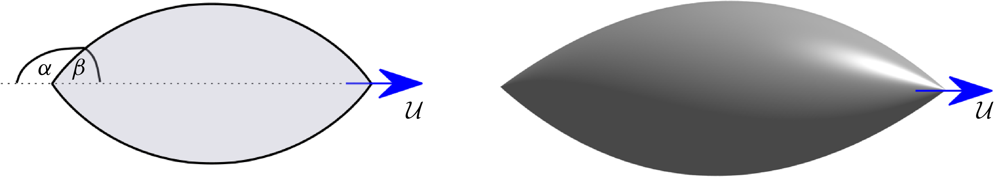


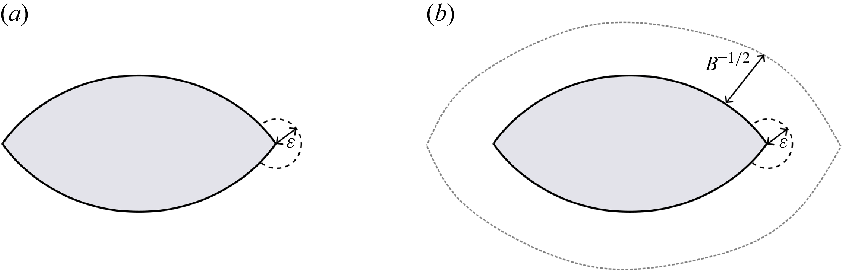


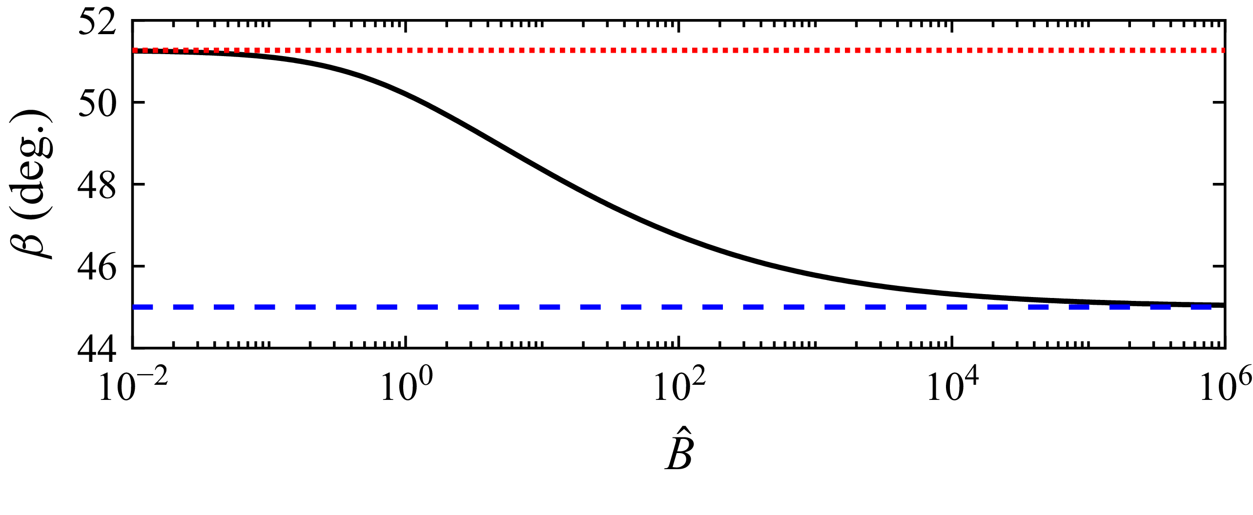


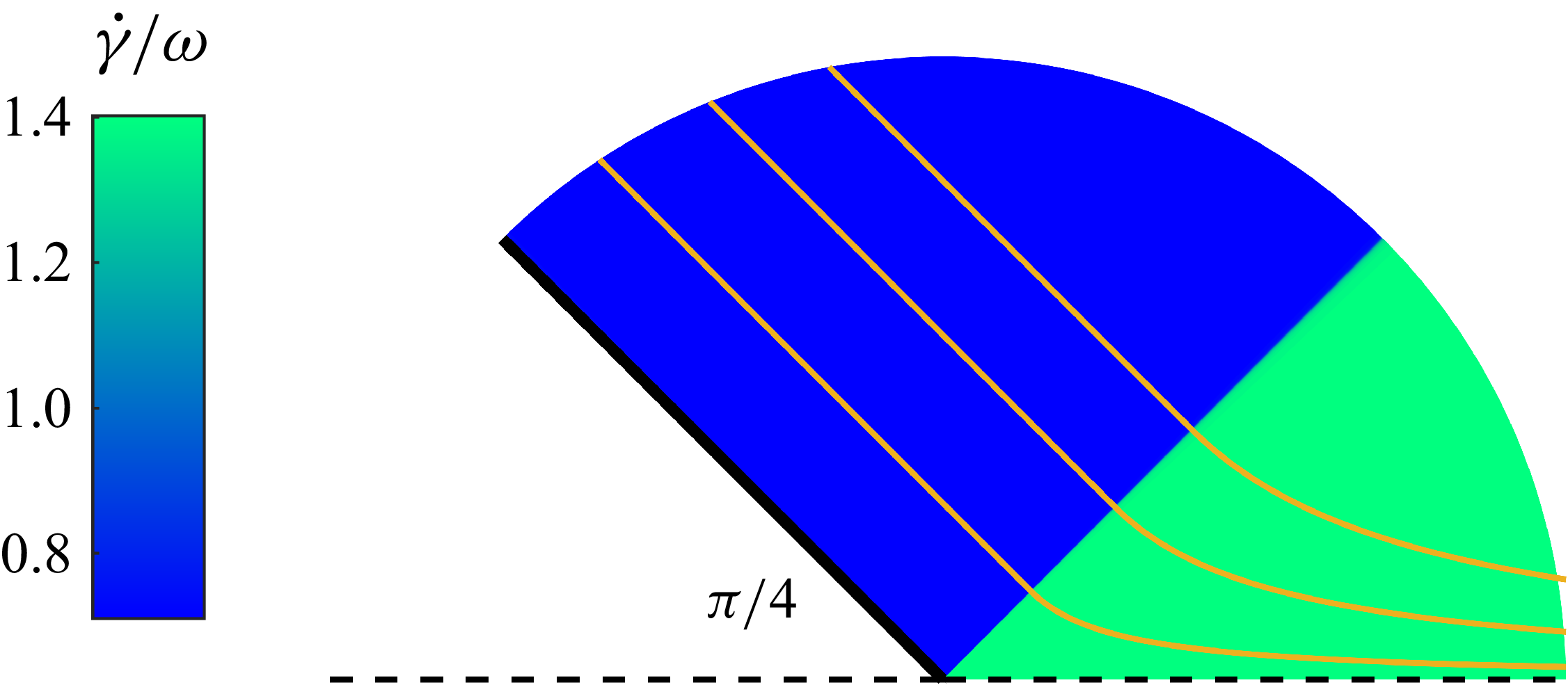


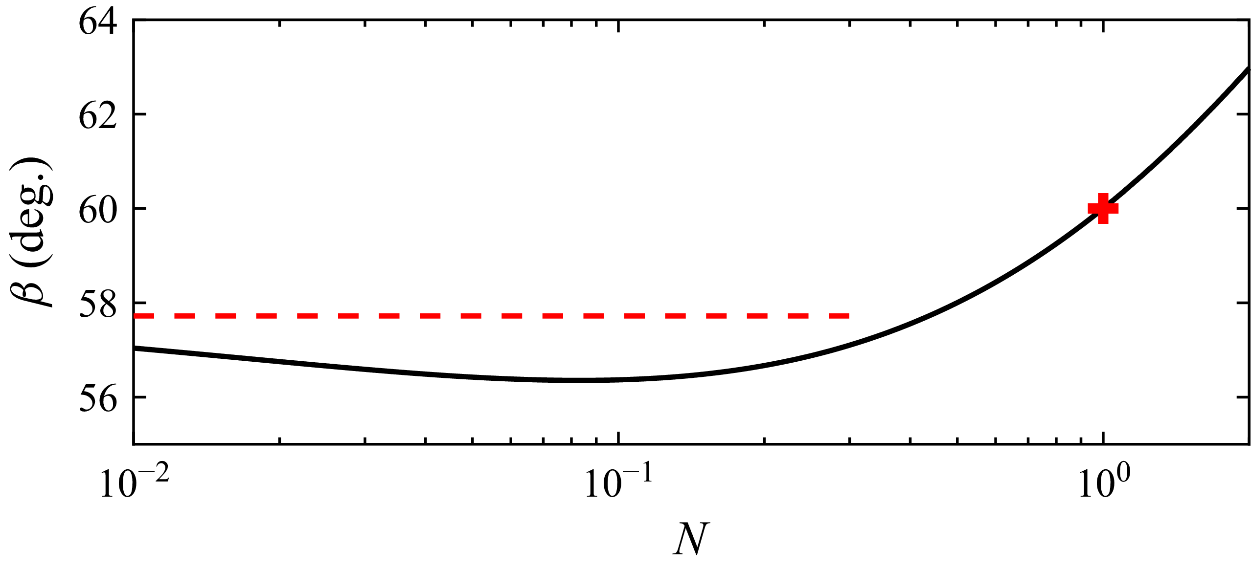


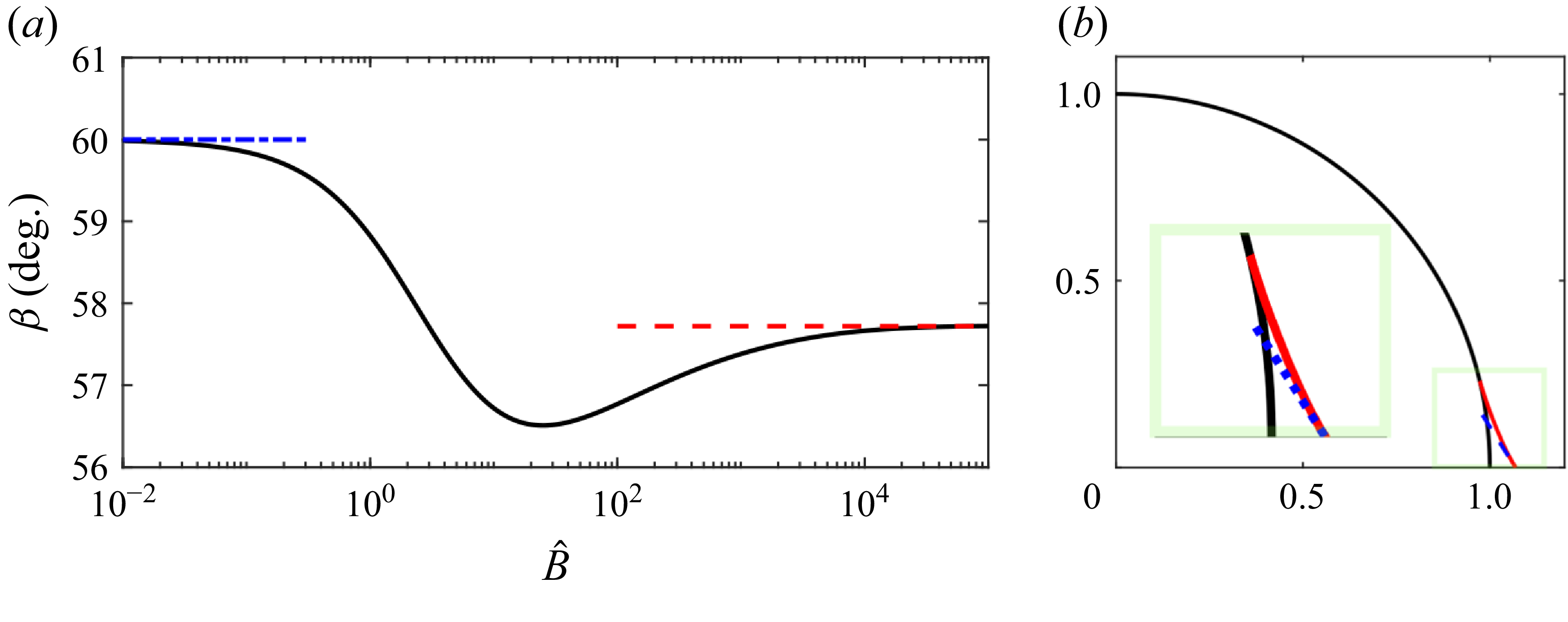


 Open access