


1. Introduction
Magnetic mirrors, or adiabatic traps, present a compelling avenue for plasma confinement through the deflection of particles away from high-field regions. In recent years, the resurgence of interest in mirrors as a fusion concept has been led by groundbreaking experiments at the collisional Gas Dynamic Trap Experiment (GDT) at the Budker Institute in Novosibirsk, Russia, which achieved unprecedented transient electron temperatures of 900 eV, demonstrating the viability of mirrors in fusion endeavours (Bagryansky et al. Reference Bagryansky, Shalashov, Gospodchikov, Lizunov, Maximov, Prikhodko, Soldatkina, Solomakhin and Yakovlev2015).
One of the most remarkable results from the GDT experiment is the stabilisation of axisymmetric mirrors against the well-understood interchange instability (Post & Rosenbluth Reference Post and Rosenbluth1966). Vortex confinement, for instance, has been shown to stabilise the $m=1$
flute interchange mode, and finite Larmor radius effects can stabilise
$m=1$
flute interchange mode, and finite Larmor radius effects can stabilise $m\geqslant 2$
(Beklemishev et al. Reference Beklemishev, Bagryansky, Chaschin and Soldatkina2010; Bagryansky et al. Reference Bagryansky2011; Beklemishev Reference Beklemishev2017; Ryutov et al. Reference Ryutov, Berk, Cohen, Molvik and Simonen2011; White, Hassam & Brizard Reference White, Hassam and Brizard2018). Moreover, recent advancements in superconducting magnet technology and electron cyclotron heating (ECH) have motivated new experiments to extend the results of GDT (Fowler, Moir & Simonen Reference Fowler, Moir and Simonen2017). One such experiment is the Wisconsin high-field axisymmetric mirror experiment (WHAM) in Madison, Wisconsin (Egedal et al. Reference Egedal, Endrizzi, Forest and Fowler2022; Endrizzi et al. Reference Endrizzi2023). Their new endeavour, using high-temperature superconducting (HTS) REBCO tapes and neutral beam injection (NBI), will investigate the magnetohydrodynamic (MHD) and kinetic stability of the axisymmetric mirror, extended into the collisionless regime. With these new experimental techniques and MHD stability in sight, questions arise related to particle and energy confinement in these new stable axisymmetric mirror configurations.
$m\geqslant 2$
(Beklemishev et al. Reference Beklemishev, Bagryansky, Chaschin and Soldatkina2010; Bagryansky et al. Reference Bagryansky2011; Beklemishev Reference Beklemishev2017; Ryutov et al. Reference Ryutov, Berk, Cohen, Molvik and Simonen2011; White, Hassam & Brizard Reference White, Hassam and Brizard2018). Moreover, recent advancements in superconducting magnet technology and electron cyclotron heating (ECH) have motivated new experiments to extend the results of GDT (Fowler, Moir & Simonen Reference Fowler, Moir and Simonen2017). One such experiment is the Wisconsin high-field axisymmetric mirror experiment (WHAM) in Madison, Wisconsin (Egedal et al. Reference Egedal, Endrizzi, Forest and Fowler2022; Endrizzi et al. Reference Endrizzi2023). Their new endeavour, using high-temperature superconducting (HTS) REBCO tapes and neutral beam injection (NBI), will investigate the magnetohydrodynamic (MHD) and kinetic stability of the axisymmetric mirror, extended into the collisionless regime. With these new experimental techniques and MHD stability in sight, questions arise related to particle and energy confinement in these new stable axisymmetric mirror configurations.
Parallel losses play a critical role in the confinement of particles and energy, which occur when particles scatter due to collisions across the loss cone (Berk & Chen Reference Berk and Chen1988). Pastukhov (Reference Pastukhov1974) laid the foundation for calculating parallel losses in a magnetic mirror with the method of images approach that this study uses. Pastukhov’s insight showed that the steady-state balance among a low-energy source, Fokker–Planck collision operator and high-energy image sinks could be simplified by transforming the problem into an analogous Poisson equation, then solved using standard techniques from electromagnetism (Jackson Reference Jackson1999). Building on Pastukhov’s insight, Najmabadi, Conn & Cohen (Reference Najmabadi, Conn and Cohen1984) extended the analysis by simplifying Pastukhov’s variable transformations, reducing the number of approximations made, and including a higher-order correction, yielding a more refined solution. Recent advancements have been made by Ochs, Munirov & Fisch (Reference Ochs, Munirov and Fisch2023), who included relativistic effects to Najmabadi’s approach.
Although parallel dynamics is often the fastest time scale phenomenon in magnetised plasmas, many researchers are interested in studying the next-order perpendicular transport due to micro-stability and turbulence, which find their best answers in computer simulations that include collisions. With the recent investigations using the Gkeyll code to study high-field magnetic mirrors using the Dougherty collision operator (Francisquez et al. Reference Francisquez, Rosen, Mandell, Hakim, Forest and Hammett2023), it is essential to understand the effect of this approximate collision operator on parallel collisional losses before it is extended to study perpendicular transport.
To understand the key details and trade-offs between different collision operators, we must first study a few important approximations in this context. A comprehensive description of two-particle collisions within the framework of a Fokker–Planck operator involves the so-called ‘Rosenbluth potentials’ (Rosenbluth et al. Reference Rosenbluth, MacDonald and Judd1957). This fully fledged operator, while widely studied and implemented, poses computational and analytical challenges (Taitano et al. Reference Taitano, Chacón, Simakov and Molvig2015). In some cases, approximations become a pragmatic necessity to render the problem computationally tractable. In this context, one widely used approximate collision operator is the Lenard–Bernstein (LBO) / Dougherty operator: a simple operator that captures the advection and diffusion responses from small-angle two-body collisions (Lenard & Bernstein Reference Lenard and Bernstein1958; Dougherty Reference Dougherty1964). The difference between the LBO and Dougherty collision operators is that the LBO has zero parallel streaming fluid flow velocity, while the Dougherty operator includes the parallel fluid flow velocity in calculating the drag, useful for cases where momentum conservation is important.
Novel work was performed using the Gkeyll code in projecting the Dougherty operator onto a discontinuous Galerkin framework with enhanced multi-species collisions for gyrokinetic and Vlasov–Maxwell simulations (Hakim et al. Reference Hakim, Francisquez, Juno and Hammett2020; Francisquez et al. Reference Francisquez, Bernard, Mandell, Hammett and Hakim2020, Reference Francisquez, Juno, Hakim, Hammett and Ernst2022). Owing to the Dougherty operator having eigenfunctions of Hermite polynomials, the GX code uses this simple collision operator (Mandell et al. Reference Mandell, Dorland, Abel, Gaur, Kim, Martin and Qian2022). The GENE-X code can simulate x-point geometry tokamak configurations, with their most rigorous collision operator being Dougherty (Ulbl et al. Reference Ulbl, Michels and Jenko2022, Reference Ulbl, Body, Zholobenko, Stegmeir, Pfennig and Jenko2023). Other examples of plasma kinetic / gyrokinetic codes that have implemented such collision operators (at least as an option) include Ye et al. (Reference Ye, Hu, Shu and Zhong2024), Celebre, Servidio & Valentini (Reference Celebre, Servidio and Valentini2023), Hoffmann, Frei & Ricci (Reference Hoffmann, Frei and Ricci2023), Frei, Hoffmann & Ricci (Reference Frei, Hoffmann and Ricci2022), Perrone, Jorge & Ricci (Reference Perrone, Jorge and Ricci2020), Loureiro et al. (Reference Loureiro, Dorland, Fazendeiro, Kanekar, Mallet, Vilelas and Zocco2016), Grandgirard et al. (Reference Grandgirard2016), Pezzi, Camporeale & Valentini (Reference Pezzi, Camporeale and Valentini2016), Parker & Dellar (Reference Parker and Dellar2015) and Hatch et al. (Reference Hatch, Jenko, Bañón Navarro and Bratanov2013). An LBO / Dougherty collision operator with the appropriate definitions satisfies many properties of a good collision operator, such as conservation of density, momentum and energy (Francisquez et al. Reference Francisquez, Bernard, Mandell, Hammett and Hakim2020). The most significant defect in this model is that the collision frequency is independent of velocity, leading to inaccurate results in the tail of the distribution function. Furthermore, the operator’s isotropic diffusion coefficient makes no distinction between pitch-angle scattering and energy diffusion (Hirshman & Sigmar Reference Hirshman and Sigmar1976). Some of the shortcomings of the Lenard–Bernstein / Dougherty operator are described by Knyazev, Dorf & Krasheninnikov (Reference Knyazev, Dorf and Krasheninnikov2023).
In this study, we build upon the method of images approach developed by Najmabadi et al. (Reference Najmabadi, Conn and Cohen1984), but with a focus on the LBO, since we consider a system with zero parallel fluid flow. Since the ambipolar potential of magnetic mirrors shifts the loss cone towards higher-energy particles, we must investigate the validity of the LBO’s collisionality approximation at high energies. Following the method of images approach from Najmabadi et al. (Reference Najmabadi, Conn and Cohen1984), results show that the particle confinement time scales as $a \exp (a^2)$
using the LBO, in contrast to the scaling
$a \exp (a^2)$
using the LBO, in contrast to the scaling $a^2 \exp (a^2)$
that more accurate Coulomb collision operator yields, where
$a^2 \exp (a^2)$
that more accurate Coulomb collision operator yields, where $a^2$
is proportional to the ambipolar potential. In addition, the average energy of lost particles is also modified. The error between the average energy of lost particles and our numerical solver is comparable to that in the study of Najmabadi et al. (Reference Najmabadi, Conn and Cohen1984). It is critical that a code using the LBO or Dougherty collision operator matches particle loss rates compared with an experiment to predict the correct ambipolar potential. Suggestions are made to reduce the collision frequency to match particle loss rates compared with the results of Najmabadi et al. (Reference Najmabadi, Conn and Cohen1984).
$a^2$
is proportional to the ambipolar potential. In addition, the average energy of lost particles is also modified. The error between the average energy of lost particles and our numerical solver is comparable to that in the study of Najmabadi et al. (Reference Najmabadi, Conn and Cohen1984). It is critical that a code using the LBO or Dougherty collision operator matches particle loss rates compared with an experiment to predict the correct ambipolar potential. Suggestions are made to reduce the collision frequency to match particle loss rates compared with the results of Najmabadi et al. (Reference Najmabadi, Conn and Cohen1984).
It is of interest to mention and discuss an alternative to the method of images approach, as the historical journey towards accurate ambipolar estimates encompasses diverse approaches. Chernin & Rosenbluth (Reference Chernin and Rosenbluth1978) introduced an alternative derivation that approximates the loss cone as a square in velocity space, yielding insights using a linearised Fokker–Planck equation and the associated variational principle. Cohen et al. (Reference Cohen, Rensink, Cutler and Mirin1978) showed that the techniques of Chernin & Rosenbluth (Reference Chernin and Rosenbluth1978) lacked robustness compared with Pastukhov’s technique, and higher-order approximations were needed. Subsequent work by Catto & Bernstein (Reference Catto and Bernstein1981), followed by Catto & Li (Reference Catto and Li1985) and Fyfe et al. (Reference Fyfe, Weiser, Bernstein, Eisenstat and Schultz1981), refined this approach by eliminating the square loss cone approximation and extending the approach to higher order. Catto’s studies circumvent the need for an accurate solution for the distribution function by transforming the problem into parallel and perpendicular coordinates to the loss cone and then employing variational techniques to yield improved confinement times. Khudik (Reference Khudik1997) demonstrated the comparable accuracy of fourth-order extensions of Catto’s methods to Najmabadi’s approach. Furthermore, these variational methods generalise to arbitrary mirror ratios and, therefore, would be more suitable for application to toroidal confinement devices, which have order unity mirror ratios. Extending these models to the LBO would not be trivial because these methods are finely tuned to the Coulomb operator. Although these methods have many good properties, we are ultimately interested in large mirror ratios, and the flexibility of variational techniques is unnecessary.
Subsequent sections will use the method of images approach to explore how the LBO collision operator changes the parallel losses of a magnetic mirror. In § 2, the problem is presented and solved systematically for the confinement time and energy loss rate. A correction factor is evaluated numerically in § 3. Results are compared with the numerical code presented in § 3. This approach’s validity and applicability to mirror simulation codes are discussed in § 4. Suggestions are made for modifying the collision frequency to obtain the appropriate ambipolar potential. Finally, we conclude in § 5.
2. Method of images solution
Our solution follows closely with the methods of Najmabadi et al. (Reference Najmabadi, Conn and Cohen1984) with some key differences. In a single-particle picture of a magnetic mirror, the parallel dynamics of particle losses depend on whether they possess sufficient energy to overcome the confining forces. These forces arise from gradients in the magnetic field magnitude $(\vec \nabla B)$
and an electrostatic ambipolar potential (
$(\vec \nabla B)$
and an electrostatic ambipolar potential ( $z_s e\phi$
), where
$z_s e\phi$
), where $e$
is the elementary charge and
$e$
is the elementary charge and $z_s$
is the charge number of species
$z_s$
is the charge number of species $s$
. When particles have enough energy to overcome the
$s$
. When particles have enough energy to overcome the $\vec \nabla B$
forces in the absence of an ambipolar potential, they reside within a specific region in phase space known as the ‘loss cone’. The introduction of an ambipolar potential alters the minimum energy required for escape, thereby transforming the loss cone into a ‘loss hyperboloid’. The loss hyperboloid can be expressed as
$\vec \nabla B$
forces in the absence of an ambipolar potential, they reside within a specific region in phase space known as the ‘loss cone’. The introduction of an ambipolar potential alters the minimum energy required for escape, thereby transforming the loss cone into a ‘loss hyperboloid’. The loss hyperboloid can be expressed as
 \begin{align} 1-\mu ^2 = \frac {1}{R} \left ( 1 - \frac {v_0^2}{v^2} \right). \end{align}
Loss boundary in velocity space for electrostatically confined particles in a magnetic mirror field. Imposed on the figure is a model depiction of the low energy source. The dotted green line represents the sinks used to solve for the distribution function. The blue line is the loss hyperboloid described in (2.1), and the red dashed line is the loss cone without an ambipolar potential.

Here, $\mu = \cos \theta = v_{||} / v$
is the cosine of the pitch angle,
$\mu = \cos \theta = v_{||} / v$
is the cosine of the pitch angle, $v$
is the total velocity
$v$
is the total velocity $|\vec {v}|$
,
$|\vec {v}|$
, $v_{||} = \left (\vec {v} \cdot \vec {B} \right) / B$
is the component of the velocity parallel to the magnetic field,
$v_{||} = \left (\vec {v} \cdot \vec {B} \right) / B$
is the component of the velocity parallel to the magnetic field, $R$
is the ratio of the maximum magnetic field to the minimum magnetic field
$R$
is the ratio of the maximum magnetic field to the minimum magnetic field $B_{{max}}/B_{{min}}$
and
$B_{{max}}/B_{{min}}$
and $v_0$
is the loss velocity corresponding to the ambipolar potential (
$v_0$
is the loss velocity corresponding to the ambipolar potential ( $m_s v_0^2 /2 = z_s e \phi$
), where
$m_s v_0^2 /2 = z_s e \phi$
), where $m_s$
is mass. The goal is to recreate this boundary, where the distribution function is null, with image sources and sinks. A model of the loss hyperboloid, source and image sinks in the problem is shown in figure 1. A source is placed at a low velocity, in a steady-state balance with the collision operator, while sinks are placed in the loss region and
$m_s$
is mass. The goal is to recreate this boundary, where the distribution function is null, with image sources and sinks. A model of the loss hyperboloid, source and image sinks in the problem is shown in figure 1. A source is placed at a low velocity, in a steady-state balance with the collision operator, while sinks are placed in the loss region and $f_s$
is extended. With these sinks, the equation for
$f_s$
is extended. With these sinks, the equation for $f_s$
near the loss hyperboloid is
$f_s$
near the loss hyperboloid is
 \begin{equation} \mathcal{L}(f_s) + Q(v,\mu) = 0. \end{equation}
Here, $\mathcal{L}(f_s)$
is a collision operator, which acts on the distribution function
$\mathcal{L}(f_s)$
is a collision operator, which acts on the distribution function $f_s$
of species
$f_s$
of species $s$
, and
$s$
, and $Q(v,\mu)$
is an image sink of particles placed inside the loss region, where
$Q(v,\mu)$
is an image sink of particles placed inside the loss region, where $f_s$
is extended. The sink
$f_s$
is extended. The sink $Q$
will be chosen to make
$Q$
will be chosen to make $f_s = 0$
at the loss hyperboloid’s vertex defined by (2.1) as well as have the contour of
$f_s = 0$
at the loss hyperboloid’s vertex defined by (2.1) as well as have the contour of $f_s = 0$
match the radii of curvature of the loss hyperboloid at the vertex. Thus, the boundary conditions on
$f_s = 0$
match the radii of curvature of the loss hyperboloid at the vertex. Thus, the boundary conditions on $f_s$
are defined as
$f_s$
are defined as
 \begin{align} &f_s({v},\mu)|_{v={v}_0,\mu =\pm 1} = 0, &\frac {\partial _{{v}} f_s}{\partial _\mu f_s}\bigg \rvert _{{v}=v_0,\mu =\pm 1} = \frac {1}{R {v}_0}. \ \end{align}
For small $v$
, we assume that
$v$
, we assume that $f_s$
is a Maxwellian,
$f_s$
is a Maxwellian,
 \begin{align} f_s(v,\mu) |_{v \rightarrow 0} \rightarrow \frac {n_s}{\pi ^{3/2} v_{th,s}^2} \exp\! (\!-\frac {v^2}{v_{th,s}^2}), \end{align}
where $n_s$
is number density,
$n_s$
is number density, $v_{th,s} = \sqrt {2T_s / m_s}$
,
$v_{th,s} = \sqrt {2T_s / m_s}$
, $T_s$
is temperature in units of energy and
$T_s$
is temperature in units of energy and $v$
is the total magnitude of the velocity
$v$
is the total magnitude of the velocity $|\vec {v}|$
. Assuming a square-well approximation for the magnetic field and considering that the maximum magnetic field occurs at the mirror throat, the LBO has the form (Lenard & Bernstein Reference Lenard and Bernstein1958)
$|\vec {v}|$
. Assuming a square-well approximation for the magnetic field and considering that the maximum magnetic field occurs at the mirror throat, the LBO has the form (Lenard & Bernstein Reference Lenard and Bernstein1958)
 \begin{equation} \mathcal{L}(f_s) = \nu _{sLBO}\frac {\partial }{\partial \vec {v}} \cdot \left ( \vec {v} f_s + \frac {v_{th,s}^2}{2} \frac {\partial f_s}{\partial \vec {v}} \right), \end{equation}
where $\nu _{sLBO}$
is the collision frequency used in the LBO,
$\nu _{sLBO}$
is the collision frequency used in the LBO, $\vec {v}$
is a velocity vector and
$\vec {v}$
is a velocity vector and $v_{th,s}$
is the thermal velocity. Generality is left in defining the collision frequency
$v_{th,s}$
is the thermal velocity. Generality is left in defining the collision frequency $\nu _{sLBO}$
because it may be chosen to match certain important physical quantities and rates in its specific implementation (Francisquez et al. Reference Francisquez, Juno, Hakim, Hammett and Ernst2022). For instance, one may choose the collision frequency for the LBO to match thermal equilibration rates, Braginskii heat fluxes or the Spitzer resistivity. Later in this work, we will investigate choosing the LBO’s collision frequency to match ambipolar collisional losses from a magnetic mirror field. To simplify the analysis, we adopt the following normalisations and definitions:
$\nu _{sLBO}$
because it may be chosen to match certain important physical quantities and rates in its specific implementation (Francisquez et al. Reference Francisquez, Juno, Hakim, Hammett and Ernst2022). For instance, one may choose the collision frequency for the LBO to match thermal equilibration rates, Braginskii heat fluxes or the Spitzer resistivity. Later in this work, we will investigate choosing the LBO’s collision frequency to match ambipolar collisional losses from a magnetic mirror field. To simplify the analysis, we adopt the following normalisations and definitions:
 \begin{align} \bar {v} &= \frac {v}{v_{th,s}}; & F_s &= \frac {v_{th,s}^3 f_s}{n_s}. \end{align}
Our normalisation $\bar {v}$
is what Pastukhov (Reference Pastukhov1974) and others refer to as
$\bar {v}$
is what Pastukhov (Reference Pastukhov1974) and others refer to as $x$
. We restate the LBO in normalised spherical coordinates to improve clarity,
$x$
. We restate the LBO in normalised spherical coordinates to improve clarity,
 \begin{equation} \mathcal{L}(F_s) = \frac {1}{\bar {v}^2} \frac {\partial }{\partial \bar {v}} \bar {v}^3 \left ( F_s + \frac {1}{2\bar {v}} \frac {\partial F_s}{\partial \bar {v}}\right) + \frac {Z_s}{2 \bar {v}^2} \frac {\partial }{\partial \mu } \left ( 1 - \mu ^2 \right) \frac {\partial F_s}{\partial \mu }. \end{equation}
We introduce a factor $Z_s$
into the diffusion term to correct for the LBO’s approximation of treating the pitch-angle scattering and energy diffusion terms equally. Although for the LBO
$Z_s$
into the diffusion term to correct for the LBO’s approximation of treating the pitch-angle scattering and energy diffusion terms equally. Although for the LBO $Z_s=1$
, an opportunity is left for future work to correct this defect by modifying the coefficient
$Z_s=1$
, an opportunity is left for future work to correct this defect by modifying the coefficient $Z_s$
. The factor of 2 in the pitch-angle scattering in (2.7) comes from the
$Z_s$
. The factor of 2 in the pitch-angle scattering in (2.7) comes from the $1/2$
in the
$1/2$
in the $v_{th,s}^2$
term in (2.5). An essential distinction between (2.7) and the collision operators proposed by Pastukhov (Reference Pastukhov1974) and Najmabadi et al. (Reference Najmabadi, Conn and Cohen1984) lies in the factors of
$v_{th,s}^2$
term in (2.5). An essential distinction between (2.7) and the collision operators proposed by Pastukhov (Reference Pastukhov1974) and Najmabadi et al. (Reference Najmabadi, Conn and Cohen1984) lies in the factors of $\bar {v}$
. The collision operators in their work retain the velocity dependence within the Rosenbluth potentials. Below are the collision operators from Pastukhov (Reference Pastukhov1974) and Najmabadi et al. (Reference Najmabadi, Conn and Cohen1984),
$\bar {v}$
. The collision operators in their work retain the velocity dependence within the Rosenbluth potentials. Below are the collision operators from Pastukhov (Reference Pastukhov1974) and Najmabadi et al. (Reference Najmabadi, Conn and Cohen1984),
 \begin{align} \mathcal{L}_{{Najmabadi}}(F_s) &= \frac {1}{\bar {v}^2} \frac {\partial }{\partial \bar {v}} \left ( F_s + \frac {1}{2 \bar {v}} \frac {\partial F_s}{\partial \bar {v}}\right) + \frac {1}{\bar {v}^3} \left ( Z_{s,N} - \frac {1}{4 \bar {v}^2}\right)\frac {\partial }{\partial \mu } \left ( 1 - \mu ^2 \right) \frac {\partial F_s}{\partial \mu }, \end{align}
 \begin{align} \mathcal{L}_{{Pastukhov}}(F_s) &= \frac {1}{\bar {v}^2} \frac {\partial }{\partial \bar {v}} \left ( F_s + \frac {1}{2 \bar {v}} \frac {\partial F_s}{\partial \bar {v}}\right) + \frac {1}{\bar {v}^3} \frac {\partial }{\partial \mu } \left ( 1 - \mu ^2 \right) \frac {\partial F_s}{\partial \mu },\\[8pt]\nonumber \end{align}
where $Z_{s,N}$
is the
$Z_{s,N}$
is the $Z$
that is used by Najmabadi et al. (Reference Najmabadi, Conn and Cohen1984) and
$Z$
that is used by Najmabadi et al. (Reference Najmabadi, Conn and Cohen1984) and $N$
stands for Najmabadi et al. (Reference Najmabadi, Conn and Cohen1984), detailed in Appendix B. To compare, the collision operator used by Pastukhov (Reference Pastukhov1974) treats the factor in (2.8)
$N$
stands for Najmabadi et al. (Reference Najmabadi, Conn and Cohen1984), detailed in Appendix B. To compare, the collision operator used by Pastukhov (Reference Pastukhov1974) treats the factor in (2.8) $\left (Z_{s,N} - 1/(4 \bar {v}^2)\right)$
as one, although Cohen et al. (Reference Cohen, Freis and Newcomb1986) addresses this limitation in treating the multi-species collisions. Comparing (2.8) and (2.7), we see that the drag and parallel diffusion are missing the
$\left (Z_{s,N} - 1/(4 \bar {v}^2)\right)$
as one, although Cohen et al. (Reference Cohen, Freis and Newcomb1986) addresses this limitation in treating the multi-species collisions. Comparing (2.8) and (2.7), we see that the drag and parallel diffusion are missing the $1/\bar {v}^3$
scaling of the more accurate collision operators. However, the pitch angle scattering term is not as bad, scaling as
$1/\bar {v}^3$
scaling of the more accurate collision operators. However, the pitch angle scattering term is not as bad, scaling as $1/\bar {v}^2$
for the LBO and as
$1/\bar {v}^2$
for the LBO and as $1/\bar {v}^3$
for the more accurate operators.
$1/\bar {v}^3$
for the more accurate operators.
To simplify the solution, we define a general form for the image problem. We impose that the image sinks start at velocity $a$
, are placed solely outside the loss hyperboloid (
$a$
, are placed solely outside the loss hyperboloid ( $a \gt \bar {v}_0$
where
$a \gt \bar {v}_0$
where $\bar {v}_0^2 = z_s e \phi / T_s$
) and are isolated to lie along
$\bar {v}_0^2 = z_s e \phi / T_s$
) and are isolated to lie along $\mu = \pm 1$
to preserve the symmetry of the problem. As described in figure 1,
$\mu = \pm 1$
to preserve the symmetry of the problem. As described in figure 1,
 \begin{equation} Q(\bar {v},\mu) = -\frac {\delta (1-\mu ^2)}{4\pi } H(\bar {v}-a) q(\bar {v}), \end{equation}
where $H()$
is the Heaviside step function and
$H()$
is the Heaviside step function and $\delta ()$
is the Dirac delta function.
$\delta ()$
is the Dirac delta function.
Pastukhov (Reference Pastukhov1974) assume a form for the sinks $q(\bar {v}) = q_0 \exp (-\bar {v}^2)$
, but the later work by Najmabadi et al. (Reference Najmabadi, Conn and Cohen1984) shows that defining
$q(\bar {v}) = q_0 \exp (-\bar {v}^2)$
, but the later work by Najmabadi et al. (Reference Najmabadi, Conn and Cohen1984) shows that defining $q(\bar {v}) = q_0 \exp (-\bar {v}^2) (Z_a - 1/4 \bar {v}^2)/ \bar {v}^3$
makes the resultant equations simpler to solve with fewer approximations. Najmabadi et al. (Reference Najmabadi, Conn and Cohen1984) finds the form of
$q(\bar {v}) = q_0 \exp (-\bar {v}^2) (Z_a - 1/4 \bar {v}^2)/ \bar {v}^3$
makes the resultant equations simpler to solve with fewer approximations. Najmabadi et al. (Reference Najmabadi, Conn and Cohen1984) finds the form of $q(\bar {v})$
by leaving its functional form free during the problem set-up, then choosing a specific form at a later stage to facilitate a solution. Thus, we choose to leave the form of
$q(\bar {v})$
by leaving its functional form free during the problem set-up, then choosing a specific form at a later stage to facilitate a solution. Thus, we choose to leave the form of $q(\bar {v})$
arbitrary in (2.10) and will define its form at a later stage.
$q(\bar {v})$
arbitrary in (2.10) and will define its form at a later stage.
Without approximation, we can use (2.7) to rewrite (2.2) in the following way:
 \begin{equation} \frac {2 e^{\bar {v}^2}}{\bar {v}} \frac {\partial }{\partial e^{\bar {v}^2}} \bar {v}^3 \frac {\partial }{\partial e^{\bar {v}^2}} \left ( e^{\bar {v}^2} F_s \right) + \frac {Z_s}{2 \bar {v}^2} \frac {\partial }{\partial \mu } \left ( 1 - \mu ^2 \right) \frac {\partial F_s}{\partial \mu } + Q(\bar {v},\mu) = 0. \end{equation}
The inverse chain rule is used to absorb factors of $\bar {v}$
into the derivatives and we also employ the identity
$\bar {v}$
into the derivatives and we also employ the identity $ F_s + (1/ 2 \bar {v}) \partial _{\bar {v}} F_s = (1/ 2 \bar {v}) \exp {(\!-\bar {v}^2)}\partial _{\bar {v}} (\exp {(\bar {v}^2)} F_s)$
. Let us define here the variable transformation
$ F_s + (1/ 2 \bar {v}) \partial _{\bar {v}} F_s = (1/ 2 \bar {v}) \exp {(\!-\bar {v}^2)}\partial _{\bar {v}} (\exp {(\bar {v}^2)} F_s)$
. Let us define here the variable transformation $z(\bar {v})=\exp {(\bar {v}^2)}$
. We now make a critical approximation: large changes in
$z(\bar {v})=\exp {(\bar {v}^2)}$
. We now make a critical approximation: large changes in $z$
cause only small changes in
$z$
cause only small changes in $\bar {v}^2 = \ln (z)$
, making the derivatives of powers of
$\bar {v}^2 = \ln (z)$
, making the derivatives of powers of $\bar {v}$
small. This justifies moving the
$\bar {v}$
small. This justifies moving the $\bar {v}^3$
outside the derivative. In more detail, the approximation we make says
$\bar {v}^3$
outside the derivative. In more detail, the approximation we make says
 \begin{equation} 3 \bar {v}^2 F_s, \bar {v} \frac {\partial F_s}{\partial \bar {v}} \ll \bar {v}^3 \frac {\partial F_s}{\partial \bar {v}}, \bar {v}^3 \frac {\partial }{\partial \bar {v}} \left ( \frac {1}{2 \bar {v}} \frac {\partial F_s}{\partial \bar {v}} \right). \end{equation}
This is valid since we are only interested in $F_s$
near the loss cone at large velocities, where
$F_s$
near the loss cone at large velocities, where $\partial F_s / \partial \bar {v}$
is large and
$\partial F_s / \partial \bar {v}$
is large and $\bar {v} \ll \bar {v}^3$
. To simplify further, we define
$\bar {v} \ll \bar {v}^3$
. To simplify further, we define $g(\bar {v},\mu) = \pi ^{3/2} \exp (\bar {v}^2) F_s(\bar {v},\mu)$
to factor out the Maxwellian component of the solution. This leads to the new form
$g(\bar {v},\mu) = \pi ^{3/2} \exp (\bar {v}^2) F_s(\bar {v},\mu)$
to factor out the Maxwellian component of the solution. This leads to the new form
 \begin{align} \left ( \frac {\partial ^2}{\partial z^2} + \frac {Z_s}{4 z^2 \ln (z)^2} \frac {\partial }{\partial \mu } \left ( 1 - \mu ^2 \right) \frac {\partial }{\partial \mu } \right) g_s(\bar {v},\mu) + \frac {\pi ^{3/2}}{2 z \ln (z)} Q(\bar {v},\mu) = 0. \end{align}
We aim to make the operator on $g(\bar {v},\mu)$
resemble a cylindrical Laplacian to map this problem to a Poisson problem. For this reason, we must also perform a transformation on the pitch angle scattering component. Consider a general variable transform of the form
$g(\bar {v},\mu)$
resemble a cylindrical Laplacian to map this problem to a Poisson problem. For this reason, we must also perform a transformation on the pitch angle scattering component. Consider a general variable transform of the form $\rho (\bar {v},\mu) = h(\bar {v},\mu) \sqrt {1-\mu ^2}$
. Assuming a large mirror ratio
$\rho (\bar {v},\mu) = h(\bar {v},\mu) \sqrt {1-\mu ^2}$
. Assuming a large mirror ratio $R \gg 1$
, we may approximate that near the loss cone
$R \gg 1$
, we may approximate that near the loss cone $\mu \approx \pm 1$
. Thus, computing
$\mu \approx \pm 1$
. Thus, computing $\partial \rho / \partial \mu$
, we neglect
$\partial \rho / \partial \mu$
, we neglect $\partial h / \partial \mu$
, which would be multiplied by a term
$\partial h / \partial \mu$
, which would be multiplied by a term $(1-\mu ^2)$
, which is small. From this, we find
$(1-\mu ^2)$
, which is small. From this, we find $\partial _\mu \approx -(\mu h^2/\rho)\partial _\rho$
and
$\partial _\mu \approx -(\mu h^2/\rho)\partial _\rho$
and $(1-\mu ^2) = \rho ^2/h^2$
. Under this transformation,
$(1-\mu ^2) = \rho ^2/h^2$
. Under this transformation, $(1-\mu ^2)\partial _\mu$
becomes
$(1-\mu ^2)\partial _\mu$
becomes $- \mu \rho \partial _\rho$
without any factors of
$- \mu \rho \partial _\rho$
without any factors of $h(\bar {v}, \mu)$
.
$h(\bar {v}, \mu)$
.
Part of the elegance of this method is that we are not limited by the form of $h(\bar {v},\mu)$
, as long as
$h(\bar {v},\mu)$
, as long as $z$
is only a function of
$z$
is only a function of $\bar {v}$
. For the purpose of an argument, consider an arbitrary transformation
$\bar {v}$
. For the purpose of an argument, consider an arbitrary transformation $z(\bar {v}, \mu)$
. If
$z(\bar {v}, \mu)$
. If $\partial _\mu z$
were non-zero, we would have to use the chain rule and compute
$\partial _\mu z$
were non-zero, we would have to use the chain rule and compute $\partial _\mu \rho (z,\mu) = \partial _z \rho \, \partial _\mu z+ \partial _\mu \rho$
, thus complicating the procedure. From Najmabadi et al. (Reference Najmabadi, Conn and Cohen1984) and here, our variable transformation
$\partial _\mu \rho (z,\mu) = \partial _z \rho \, \partial _\mu z+ \partial _\mu \rho$
, thus complicating the procedure. From Najmabadi et al. (Reference Najmabadi, Conn and Cohen1984) and here, our variable transformation $z = \exp (\bar {v}^2)$
means that
$z = \exp (\bar {v}^2)$
means that $ \partial _z \rho \, \partial _\mu z = 0$
, making this variable transformation simpler. This insight is perhaps the most pivotal innovation of Najmabadi et al. (Reference Najmabadi, Conn and Cohen1984) compared with the variable transformations presented by Pastukhov (Reference Pastukhov1974). Pastukhov (Reference Pastukhov1974) uses a variable transformation
$ \partial _z \rho \, \partial _\mu z = 0$
, making this variable transformation simpler. This insight is perhaps the most pivotal innovation of Najmabadi et al. (Reference Najmabadi, Conn and Cohen1984) compared with the variable transformations presented by Pastukhov (Reference Pastukhov1974). Pastukhov (Reference Pastukhov1974) uses a variable transformation $z = \exp (\bar {v}^2) \mu / \sqrt {2 \bar {v}^2}$
and
$z = \exp (\bar {v}^2) \mu / \sqrt {2 \bar {v}^2}$
and $\rho = \exp (\bar {v}^2) \sqrt {1 - \mu ^2}$
, where both variable transformations are functions of
$\rho = \exp (\bar {v}^2) \sqrt {1 - \mu ^2}$
, where both variable transformations are functions of $\bar {v}$
and
$\bar {v}$
and $\mu$
. When ultimately satisfying boundary conditions, this leads Pastukhov (Reference Pastukhov1974) to do ‘a number of straightforward but rather cumbersome algebraic transformations’. The complications arise due to the prefactors in front of the logarithm in their (17) having a factor of
$\mu$
. When ultimately satisfying boundary conditions, this leads Pastukhov (Reference Pastukhov1974) to do ‘a number of straightforward but rather cumbersome algebraic transformations’. The complications arise due to the prefactors in front of the logarithm in their (17) having a factor of $\bar {v}/ \mu$
, which comes from the
$\bar {v}/ \mu$
, which comes from the $\mu / \bar {v}$
in their variable transformation for
$\mu / \bar {v}$
in their variable transformation for $z$
. In contrast, Najmabadi et al. (Reference Najmabadi, Conn and Cohen1984) use the variable transformations
$z$
. In contrast, Najmabadi et al. (Reference Najmabadi, Conn and Cohen1984) use the variable transformations $z = \exp (\bar {v}^2)$
and
$z = \exp (\bar {v}^2)$
and $\rho = \sqrt { 2 \bar {v}^2 / (Z_a - 1/4 \bar {v}^2)} \exp (\bar {v}^2) \tan \theta$
. Notice that, as we have pointed out above, the variable transformation in
$\rho = \sqrt { 2 \bar {v}^2 / (Z_a - 1/4 \bar {v}^2)} \exp (\bar {v}^2) \tan \theta$
. Notice that, as we have pointed out above, the variable transformation in $z$
does not depend on
$z$
does not depend on $\mu$
. The equivalent solution is (23) of Najmabadi et al. (Reference Najmabadi, Conn and Cohen1984), which is divided by a Maxwellian compared with (17) of Pastukhov (Reference Pastukhov1974). Equation (23) of Najmabadi et al. (Reference Najmabadi, Conn and Cohen1984) has a mere constant before the logarithm, making satisfying boundary conditions much simpler.
$\mu$
. The equivalent solution is (23) of Najmabadi et al. (Reference Najmabadi, Conn and Cohen1984), which is divided by a Maxwellian compared with (17) of Pastukhov (Reference Pastukhov1974). Equation (23) of Najmabadi et al. (Reference Najmabadi, Conn and Cohen1984) has a mere constant before the logarithm, making satisfying boundary conditions much simpler.
By setting $h(\bar {v},\mu)$
to cancel any factor in front of the pitch-angle scattering derivatives, it can be shown that the appropriate variable transformation is
$h(\bar {v},\mu)$
to cancel any factor in front of the pitch-angle scattering derivatives, it can be shown that the appropriate variable transformation is
 \begin{align} \rho (\bar {v},\mu) &= \frac {2 z \ln (z)}{\sqrt {Z_s}} \frac {\sqrt {1 - \mu ^2}}{\mu } = \frac {2 z \ln (z)}{\sqrt {Z_s}} \tan \theta. \end{align}
As a result, the problem is in the form of a cylindrical Poisson equation,
 \begin{align} \frac {1}{\rho } \frac {\partial }{\partial \rho } \left (\rho \frac {\partial }{\partial \rho } g_s \right) + \frac {\partial ^2 g_s}{\partial ^2 z} = \frac {\pi ^{3/2}}{2 z \ln (z)} \frac {\delta (1-\mu ^2)}{4\pi } q (\bar {v}) H(\bar {v}-a). \end{align}
We can now set the free function $q(\bar {v})$
such that the equation takes an ad hoc, easy-to-solve form,
$q(\bar {v})$
such that the equation takes an ad hoc, easy-to-solve form,
 \begin{align} \frac {1}{\rho } \frac {\partial }{\partial \rho } \left (\rho \frac {\partial }{\partial \rho } g_s \right) + \frac {\partial ^2 g_s}{\partial ^2 z}= \frac {\delta (\rho)}{2 \pi \rho } 4 \pi q_0 H(z - z_a). \end{align}
On the right-hand side of (2.16), $q_0$
is equivalent to a constant linear charge density and
$q_0$
is equivalent to a constant linear charge density and $z_a = \exp (a^2)$
. Although we choose
$z_a = \exp (a^2)$
. Although we choose $q_0$
to be a constant for the sake of having an easy-to-solve problem, it does mean we are sacrificing some detail in the ability to match (2.1) perfectly; however, exact matching is not necessary because the distribution function, as well as losses, decay at higher energies and the majority of particles are lost near the tip of the loss hyperboloid, so that is the region we are most interested in matching. By matching (2.15) and (2.16), we show in Appendix A that the appropriate connection between
$q_0$
to be a constant for the sake of having an easy-to-solve problem, it does mean we are sacrificing some detail in the ability to match (2.1) perfectly; however, exact matching is not necessary because the distribution function, as well as losses, decay at higher energies and the majority of particles are lost near the tip of the loss hyperboloid, so that is the region we are most interested in matching. By matching (2.15) and (2.16), we show in Appendix A that the appropriate connection between $q(\bar {v})$
and
$q(\bar {v})$
and $q_0$
is
$q_0$
is
 \begin{align} q(\bar {v}) = q_0 \cdot \frac {8}{\sqrt {\pi }} \frac {\mu ^2 Z_s}{z \ln (z)}. \end{align}
With the new coordinates $\rho$
and
$\rho$
and $z$
, we transform boundary condition (2.4). In addition, the lower limit of
$z$
, we transform boundary condition (2.4). In addition, the lower limit of $z=1$
for
$z=1$
for $\bar {v}=0$
is extended to
$\bar {v}=0$
is extended to $z=0$
since
$z=0$
since $z \equiv \exp (\bar {v}^2) \gg 1$
or set
$z \equiv \exp (\bar {v}^2) \gg 1$
or set $z^\prime = \exp (\bar {v}^2) - 1 = z(1 + O(\exp (-\bar {v}^2)))$
.
$z^\prime = \exp (\bar {v}^2) - 1 = z(1 + O(\exp (-\bar {v}^2)))$
.
 \begin{align} g_s(\rho,z) |_{z=0} = 1. \end{align}
Equation (2.16) with boundary condition (2.18) is solved by Jackson (Reference Jackson1999). The equivalent problem in electricity and magnetism terms is having a conducting boundary condition on the $z=0$
plane held at potential
$z=0$
plane held at potential $g_s=1$
and placing a wire of constant linear charge density
$g_s=1$
and placing a wire of constant linear charge density $q_0$
on the
$q_0$
on the $z$
-axis, suspended above the
$z$
-axis, suspended above the $z=0$
plane at height
$z=0$
plane at height $z=z_a$
. The standard method of solving this problem is to use the method of images to match the conducting boundary condition. To outline this approach, we use the method of images for the equivalent Poisson problem after previously using the method of images approach to place image sources and sinks in figure 1. This layering of the method of images is why this approach is referred to as the method of images solution for determining loss rates from a magnetic mirror. Only requiring unmapping the equation through stated variable transformations, we find the appropriate distribution function for a magnetic mirror as
$z=z_a$
. The standard method of solving this problem is to use the method of images to match the conducting boundary condition. To outline this approach, we use the method of images for the equivalent Poisson problem after previously using the method of images approach to place image sources and sinks in figure 1. This layering of the method of images is why this approach is referred to as the method of images solution for determining loss rates from a magnetic mirror. Only requiring unmapping the equation through stated variable transformations, we find the appropriate distribution function for a magnetic mirror as
 \begin{align} g_s(\rho,z) = 1 - q_0 \ln \left (\frac {z_a + z + \sqrt {\rho ^2 + \left (z_a + z\right)^2}}{z_a - z + \sqrt {\rho ^2 + \left (z_a - z\right)^2}}\right). \end{align}
Mapping this problem back to the magnetic mirror and using that $z \gg 1$
near the loss hyperboloid, we can apply the boundary conditions assigned to this problem in (2.3). Interestingly, this is the only part of the calculation in which information about the magnetic field is used in the solution. We show in Appendix C that for a general variable transformation
$z \gg 1$
near the loss hyperboloid, we can apply the boundary conditions assigned to this problem in (2.3). Interestingly, this is the only part of the calculation in which information about the magnetic field is used in the solution. We show in Appendix C that for a general variable transformation $z = \exp (\bar {v}^2)$
,
$z = \exp (\bar {v}^2)$
, $\rho = \bar \rho (\bar {v}) z \tan \theta$
, where
$\rho = \bar \rho (\bar {v}) z \tan \theta$
, where $h(\bar {v}, \mu) = \bar \rho (\bar {v}) z / \mu$
mentioned earlier, we get
$h(\bar {v}, \mu) = \bar \rho (\bar {v}) z / \mu$
mentioned earlier, we get
 \begin{align} q_0 &= \left ( \ln \left ( \frac {w+1}{w-1}\right)\right)^{-1}, \end{align}
 \begin{align} w^2 &= 1 + \frac {\bar \rho (\bar {v}_0)^2}{2 R \bar {v}_0^2} = 1 + \frac {2 \bar {v}_0^2}{ Z_s R},\\[8pt]\nonumber \end{align}
where $w = \exp (a^2 - \bar {v}_0^2)$
. This can be inverted to give
$w = \exp (a^2 - \bar {v}_0^2)$
. This can be inverted to give $a^2 = \bar {v}^2_0 + \ln (w)$
, which determines the edge of the sink region,
$a^2 = \bar {v}^2_0 + \ln (w)$
, which determines the edge of the sink region, $a$
, in terms of the tip of the loss region
$a$
, in terms of the tip of the loss region $v_0$
.
$v_0$
.
Najmabadi et al. (Reference Najmabadi, Conn and Cohen1984) adjust the strength of the sinks by examining the difference between the flux of the true loss cone, (2.1), and the approximate loss cone, where (2.19) equals zero. They account for this in their (41a) and (41b). Their instructions are to evaluate (2.19) along the loss cone one $z_se \phi / T_s$
above the tip of the loss cone in the limit where
$z_se \phi / T_s$
above the tip of the loss cone in the limit where $R \gg 1$
. This means
$R \gg 1$
. This means $\bar {v}^2 = v_0^2+1$
,
$\bar {v}^2 = v_0^2+1$
, $\mu = 1$
and
$\mu = 1$
and $a \approx v_0$
, which leads to
$a \approx v_0$
, which leads to $z = \exp (v_0^2 + 1)$
and
$z = \exp (v_0^2 + 1)$
and $\rho = 0$
, meaning
$\rho = 0$
, meaning $g(0,v_0^2+1) \approx 1 - q_0 \ln ((e+1)/(e-1)) = 1 - 0.77 q_0$
. Thus, we modify
$g(0,v_0^2+1) \approx 1 - q_0 \ln ((e+1)/(e-1)) = 1 - 0.77 q_0$
. Thus, we modify $q_0$
by subtracting
$q_0$
by subtracting $0.77$
, leading to a corrected definition of
$0.77$
, leading to a corrected definition of $q_0$
. Najmabadi et al. (Reference Najmabadi, Conn and Cohen1984) determine this to be
$q_0$
. Najmabadi et al. (Reference Najmabadi, Conn and Cohen1984) determine this to be $0.84 q_0$
, but we have not replicated the calculation used to determine their (41b),
$0.84 q_0$
, but we have not replicated the calculation used to determine their (41b),
 \begin{align} q_0 &= \left ( \ln \left ( \frac {w+1}{w-1}\right)- 0.77\right)^{-1}. \end{align}
To calculate this system’s confinement time and energy loss rate, we integrate the image sinks over all velocity space, considering the symmetry in gyro- and pitch-angle,
 \begin{align} \frac {1}{n_s \nu _{sLBO}} \frac {{\rm d}n_s}{{\rm d}t} &= 2 \pi \int _0^\infty \bar {v}^2 {\rm d}\bar {v} \int _{-1}^1 {\rm d}\mu Q(\bar {v},\mu), \end{align}
 \begin{align} \frac {3}{2}\frac {1}{\nu _{sLBO}}\frac {1}{n_s T_s} \frac {{\rm d} n_s T_s}{{\rm d}t} &= 2 \pi \int _0^\infty \bar {v}^4 {\rm d}\bar {v} \int _{-1}^1 {\rm d}\mu Q(\bar {v},\mu).\\[8pt]\nonumber\end{align}
Although this appears to be a straightforward integral, there is a subtlety to handling it worth mentioning. Equation (2.23) appears as if it is integrating over half of each delta function on both sides, but it is, in fact, integrating two whole peaks of the delta function across all of velocity space, so $\int _{-1}^1 \delta (1-\mu ^2) {\rm d}\mu = 1$
. Once we account for this intricacy, we arrive at the following forms for confinement time and energy loss rate:
$\int _{-1}^1 \delta (1-\mu ^2) {\rm d}\mu = 1$
. Once we account for this intricacy, we arrive at the following forms for confinement time and energy loss rate:
 \begin{align} \frac {1}{\tau _{c}} = \frac {1}{n_s} \frac {{\rm d}n_s}{{\rm d}t} &= -\nu _{sLBO} 2 Z_s \frac {\mathrm{Erfc}(a)}{\ln \left ( \frac {w+1}{w-1}\right)-0.77}, \end{align}
 \begin{align} \frac {1}{E_s}\frac {{\rm d}E_s}{{\rm d}t}= \frac {1}{n_s T_s} \frac {{\rm d} (n_s T_s)}{{\rm d}t} &= -\nu _{sLBO} \frac {4}{3 \sqrt {\pi }} Z_s \frac { e^{-a^2}a + \frac {\sqrt {\pi }}{2} \mathrm{Erfc}(a)}{\ln \left ( \frac {w+1}{w-1}\right)-0.77}. \\[8pt]\nonumber\end{align}
Here, $\tau _c$
is the confinement time,
$\tau _c$
is the confinement time, $E_s = 3/2 \; n_sT_s$
is total energy of the system,
$E_s = 3/2 \; n_sT_s$
is total energy of the system, $\mathrm{Erfc}()$
is the complementary error function,
$\mathrm{Erfc}()$
is the complementary error function, $w = \sqrt {1 + 2 z_s e \phi / \left ( T_s Z_s R \right)}$
and
$w = \sqrt {1 + 2 z_s e \phi / \left ( T_s Z_s R \right)}$
and $a = \sqrt { z_s e\phi / T_s + \ln {(w)}}$
.
$a = \sqrt { z_s e\phi / T_s + \ln {(w)}}$
.
We proceed to calculate the energy of the particle, but due to collisions, $z_s e \phi / T_s \sim (1/2) \ln (m_i / m_e) \gg 1$
. Furthermore, for
$z_s e \phi / T_s \sim (1/2) \ln (m_i / m_e) \gg 1$
. Furthermore, for $R \gg z_s e \phi / T_s Z_s$
,
$R \gg z_s e \phi / T_s Z_s$
, $\ln (w)$
is small, giving
$\ln (w)$
is small, giving $a \simeq \sqrt {z_s e \phi / T_s} \gg 1$
. The asymptotic expansion for a large argument of the complementary error function is
$a \simeq \sqrt {z_s e \phi / T_s} \gg 1$
. The asymptotic expansion for a large argument of the complementary error function is $\mathrm{Erfc}(x) \approx \exp (-x^2) / (\sqrt {\pi } x) \times (1 - 1/2x^2 + 3/4x^4 + \mathcal{O}(1/x^6))$
, so
$\mathrm{Erfc}(x) \approx \exp (-x^2) / (\sqrt {\pi } x) \times (1 - 1/2x^2 + 3/4x^4 + \mathcal{O}(1/x^6))$
, so $\tau _c$
scales as
$\tau _c$
scales as $a \exp (a^2)$
. The average energy of lost particles is found by evaluating
$a \exp (a^2)$
. The average energy of lost particles is found by evaluating $E_{s,{loss}} = ({\rm d}E_s/{\rm d}t)/({\rm d}n_s/{\rm d}t)$
,
$E_{s,{loss}} = ({\rm d}E_s/{\rm d}t)/({\rm d}n_s/{\rm d}t)$
,
 \begin{align} \frac {E_{s,{loss}}}{T_s} &= \frac {1}{2} \left ( 1 + \frac {2 a e^{-a^2}}{\sqrt {\pi }\mathrm{Erfc}(a)}\right) \end{align}
 \begin{align} &\approx a^2 + 1 - \frac {1}{2 a^2} + \mathcal{O}(1/a^4). \\[8pt]\nonumber\end{align}
It is important to note that (2.25) and subsequent definitions are presented in their un-normalised form. During the un-normalisation process, all quantities are stated in terms of the temperature $T_s$
of the species. This avoids confusion when using a different normalisation procedure for the thermal velocity.
$T_s$
of the species. This avoids confusion when using a different normalisation procedure for the thermal velocity.
3. Numerical simulations and corrections to (2.20)
We compare our approximate expressions for the loss rates in magnetic mirrors to results obtained using a code based on the work of Ochs et al. (Reference Ochs, Munirov and Fisch2023). The code uses the FEniCS DolfinX Python package to employ the finite element method (FEM) with third-order continuous Galerkin discretisation to solve a general Fokker–Planck model collision operator. The FEM code is meshed over the upper right quadrant of $\bar {v},\theta$
space and has a low-energy source of the form
$\bar {v},\theta$
space and has a low-energy source of the form $\bar {v}^2 \exp (\!-\bar {v}^2 / \bar {v}^2_{s0}) \theta ^2 (\pi / 2 - \theta)^2$
.Footnote
1
Here,
$\bar {v}^2 \exp (\!-\bar {v}^2 / \bar {v}^2_{s0}) \theta ^2 (\pi / 2 - \theta)^2$
.Footnote
1
Here, $\bar {v}$
is normalised velocity and
$\bar {v}$
is normalised velocity and $\theta$
is pitch angle. The normalised thermal velocity for the source is evaluated at
$\theta$
is pitch angle. The normalised thermal velocity for the source is evaluated at $\bar {v}_{s0} = 0.2$
to concentrate it at low energy. This source form is chosen to go to zero on the boundaries smoothly (the precise form of the source term has little effect on the results in the asymptotic limit
$\bar {v}_{s0} = 0.2$
to concentrate it at low energy. This source form is chosen to go to zero on the boundaries smoothly (the precise form of the source term has little effect on the results in the asymptotic limit $z_s e \phi / T_e \gg 1$
). Zero-flux boundary conditions are used at
$z_s e \phi / T_e \gg 1$
). Zero-flux boundary conditions are used at $\theta =0$
,
$\theta =0$
, $\theta =\pi /2$
,
$\theta =\pi /2$
, $v=0$
and
$v=0$
and $v=v_{max}$
, the maximal velocity extent in the problem. A resolution of
$v=v_{max}$
, the maximal velocity extent in the problem. A resolution of $\Delta \theta = \Delta \bar {v} = 0.1$
is chosen, with double resolution near the source and along the loss boundary. The boundary condition on the loss hyperboloid is Dirichlet (
$\Delta \theta = \Delta \bar {v} = 0.1$
is chosen, with double resolution near the source and along the loss boundary. The boundary condition on the loss hyperboloid is Dirichlet ( $f_s = 0$
). The domain is extended
$f_s = 0$
). The domain is extended $\sqrt {7 + z_s e \phi / T_s}$
past the loss hyperboloid vertex. An example mesh is shown in figure 2 for demonstration. An astute reader will notice that the slope of the loss hyperboloid boundary is not vertical at
$\sqrt {7 + z_s e \phi / T_s}$
past the loss hyperboloid vertex. An example mesh is shown in figure 2 for demonstration. An astute reader will notice that the slope of the loss hyperboloid boundary is not vertical at $\bar {v} = 1$
. At the tip of the loss hyperboloid, the code struggles to mesh the boundary because it is purely vertical. A finite step in
$\bar {v} = 1$
. At the tip of the loss hyperboloid, the code struggles to mesh the boundary because it is purely vertical. A finite step in $\bar {v}$
is taken and the loss boundary is linearly interpolated from the tip of the loss hyperboloid to the first point. This plot was done with a coarser resolution to see the grid. The final results were done at higher resolution confirmed to be adequate with convergence studies. The problem is solved directly using PETSc’s linear algebra solvers to find an LU decomposition.
$\bar {v}$
is taken and the loss boundary is linearly interpolated from the tip of the loss hyperboloid to the first point. This plot was done with a coarser resolution to see the grid. The final results were done at higher resolution confirmed to be adequate with convergence studies. The problem is solved directly using PETSc’s linear algebra solvers to find an LU decomposition.
An example mesh from the finite element model. Here, $z_s e \phi / T_s = 1$
and
$z_s e \phi / T_s = 1$
and $R = 2$
to exaggerate the loss cone.
$R = 2$
to exaggerate the loss cone.

To compare our numerical results to prior computational work, we need to make a key distinction between the collision operator used by our code in reproducing the results from Najmabadi et al. (Reference Najmabadi, Conn and Cohen1984) and the operators used in previous work. The results labelled ‘FEM Rosenbluth’ use a slightly modified version of the collision operator in (2.8), whereas the code used by Cohen et al. (Reference Cohen, Rensink, Cutler and Mirin1978) and later used by Najmabadi et al. (Reference Najmabadi, Conn and Cohen1984) and Fyfe et al. (Reference Fyfe, Weiser, Bernstein, Eisenstat and Schultz1981) considers a multi-species Fokker–Planck equation derived from nonlinear isotropic Rosenbluth potentials. Naive implementation of (2.8) would violate the assumption that $\bar {v} \gg 1$
because our domain also includes low velocities. The work by Cohen et al. (Reference Cohen, Rensink, Cutler and Mirin1978) avoided this issue by implementing the full nonlinear Rosenbluth potentials. To address this limitation, we approximate the parallel drag-diffusion frequency in (2.8) by using a Padé approximation of the form
$\bar {v} \gg 1$
because our domain also includes low velocities. The work by Cohen et al. (Reference Cohen, Rensink, Cutler and Mirin1978) avoided this issue by implementing the full nonlinear Rosenbluth potentials. To address this limitation, we approximate the parallel drag-diffusion frequency in (2.8) by using a Padé approximation of the form $1/\bar {v}^3 \rightarrow 1 /(1 + \bar {v}^3)$
, which asymptotically matches the high- and low-velocity Rosenbluth limits. For the pitch angle scattering component, we have a full calculation of the pitch angle scattering rate while considering collisions on a Maxwellian background to keep the problem linear. We consider two cases: a plasma with hydrogen ions and electrons, where either the ions or electrons are electrostatically confined. In both cases, the thermal velocity of electrons is much higher than the thermal velocity of the hydrogen. This results in the following collision operator:
$1/\bar {v}^3 \rightarrow 1 /(1 + \bar {v}^3)$
, which asymptotically matches the high- and low-velocity Rosenbluth limits. For the pitch angle scattering component, we have a full calculation of the pitch angle scattering rate while considering collisions on a Maxwellian background to keep the problem linear. We consider two cases: a plasma with hydrogen ions and electrons, where either the ions or electrons are electrostatically confined. In both cases, the thermal velocity of electrons is much higher than the thermal velocity of the hydrogen. This results in the following collision operator:
 \begin{equation} \mathcal{L}_{{Code}}(F_s) = \frac {1}{\bar {v}^2} \frac {\partial }{\partial \bar {v}} \frac {\bar {v}^2}{1 + \bar {v}^3} \left ( \bar {v} F_s + \frac {1}{2} \frac {\partial F_s}{\partial \bar {v}}\right) + \frac 1{\bar {v}^3} P(v) \frac {\partial }{\partial \mu } \left ( 1 - \mu ^2 \right) \frac {\partial F_s}{\partial \mu }. \end{equation}
For electrostatically confined electrons, $P(v) = (1 + \mathcal{R}(v))/2$
(
$P(v) = (1 + \mathcal{R}(v))/2$
( $Z_{s,n} = 1$
). For electrostatically confined hydrogen ions,
$Z_{s,n} = 1$
). For electrostatically confined hydrogen ions, $P(v) = \mathcal{R}(v)/2$
(
$P(v) = \mathcal{R}(v)/2$
( $Z_{s,n}=1/2$
). In these expressions,
$Z_{s,n}=1/2$
). In these expressions, $\mathcal{R}(v) = 1/(\sqrt {\pi }v) \exp (-v^2) + (1 - 1/2v^2)\rm {Erf}(v)$
and
$\mathcal{R}(v) = 1/(\sqrt {\pi }v) \exp (-v^2) + (1 - 1/2v^2)\rm {Erf}(v)$
and $\rm {Erf}$
is the error function. In contrast, the LBO model is implemented in the code without approximations as (2.7).
$\rm {Erf}$
is the error function. In contrast, the LBO model is implemented in the code without approximations as (2.7).
To demonstrate convergence, we examine increasing the resolution and the amount of the problem meshed beyond the tip of the loss hyperboloid for $z_s e \phi / T_s = 8$
and
$z_s e \phi / T_s = 8$
and $R = 10$
. When doubling all resolutions, the resultant loss rate changes by
$R = 10$
. When doubling all resolutions, the resultant loss rate changes by $-0.492\,\%$
for the Dougherty operator and
$-0.492\,\%$
for the Dougherty operator and $-1.099\,\%$
for the operator in (3.1). When not changing
$-1.099\,\%$
for the operator in (3.1). When not changing $\Delta \theta = \Delta \bar {v}$
but quadrupling the resolution near the source and along the loss hyperboloid, the loss rate changes by
$\Delta \theta = \Delta \bar {v}$
but quadrupling the resolution near the source and along the loss hyperboloid, the loss rate changes by $-0.493\,\%$
for the Dougherty operator and
$-0.493\,\%$
for the Dougherty operator and $-1.001\,\%$
for the operator in (3.1). When increasing the extents of the problem from
$-1.001\,\%$
for the operator in (3.1). When increasing the extents of the problem from $\sqrt {7 + z_s e \phi / T_s}$
to
$\sqrt {7 + z_s e \phi / T_s}$
to $\sqrt {15 + z_s e \phi / T_s}$
, the loss rate changes by
$\sqrt {15 + z_s e \phi / T_s}$
, the loss rate changes by $-0.06906\,\%$
for the Dougherty operator and
$-0.06906\,\%$
for the Dougherty operator and $-0.06732\,\%$
for the operator in (3.1). Thus, the code converges within
$-0.06732\,\%$
for the operator in (3.1). Thus, the code converges within $1\,\%$
variation for all collision operators, and this resolution is suitable for this study.
$1\,\%$
variation for all collision operators, and this resolution is suitable for this study.
In figure 3, the numerical code is validated by comparing the analytic results presented by Pastukhov (Reference Pastukhov1974) and Najmabadi et al. (Reference Najmabadi, Conn and Cohen1984) with corrections noticed by Cohen et al. (Reference Cohen, Rensink, Cutler and Mirin1978), Najmabadi et al. (Reference Najmabadi, Conn and Cohen1984), (2.25) and (2.27), which in turn were validated using other numerical methods. Results in figure 3 agree well with those in many prior works (Najmabadi et al. Reference Najmabadi, Conn and Cohen1984; Cohen et al. Reference Cohen, Rensink, Cutler and Mirin1978; Fyfe et al. Reference Fyfe, Weiser, Bernstein, Eisenstat and Schultz1981). The confinement time $\tau _c$
is normalised to collision frequency for generality. The diamonds are the finite element method numerical results and the dashed lines are the analytic approximations. Although figure 3 shows great agreement with prior work, it has a fair agreement with (2.25). To improve agreement between the code and (2.25), rather than calculating the flux correction coefficient by hand to be
$\tau _c$
is normalised to collision frequency for generality. The diamonds are the finite element method numerical results and the dashed lines are the analytic approximations. Although figure 3 shows great agreement with prior work, it has a fair agreement with (2.25). To improve agreement between the code and (2.25), rather than calculating the flux correction coefficient by hand to be $0.77$
in (2.22), we can calculate this number numerically. First, let us call this correction coefficient
$0.77$
in (2.22), we can calculate this number numerically. First, let us call this correction coefficient $c_0$
. It can be chosen to minimise error with the finite element code. Equations (2.20), (2.25) and (2.26) are modified to be the following:
$c_0$
. It can be chosen to minimise error with the finite element code. Equations (2.20), (2.25) and (2.26) are modified to be the following:
 \begin{align} \frac {1}{\tau _{c}} = \frac {1}{n_s} \frac {{\rm d}n_s}{{\rm d}t} &= -\nu _{sLBO} 2 Z_s \frac { \mathrm{Erfc}(a)}{\ln \left ( \frac {w+1}{w-1}\right) - c_0}, \end{align}
 \begin{align} \frac {1}{E_s}\frac {{\rm d}E_s}{{\rm d}t}= \frac {1}{n_s T_s} \frac {{\rm d} (n_s T_s)}{{\rm d}t} &= -\nu _{sLBO} \frac {4}{3 \sqrt {\pi }} Z_s \frac { e^{-a^2}a + \frac {\sqrt {\pi }}{2} \mathrm{Erfc}(a) }{\ln \left ( \frac {w+1}{w-1}\right) - c_0}. \\[8pt]\nonumber\end{align}
In figure 4, we show various curves that describe the error between (3.2) and the finite element code for various values of $c_0$
. This figure shows us that the value of
$c_0$
. This figure shows us that the value of $c_0$
that minimises error with the finite element code depends on the ambipolar potential and mirror ratio under investigation, although it seems to asymptote to a single value for a sufficiently large mirror ratio and ambipolar potential. In table 1, we list the appropriate correction factor to use for various values of ambipolar potential and mirror ratio that minimise error with the loss rate from the finite element code.
$c_0$
that minimises error with the finite element code depends on the ambipolar potential and mirror ratio under investigation, although it seems to asymptote to a single value for a sufficiently large mirror ratio and ambipolar potential. In table 1, we list the appropriate correction factor to use for various values of ambipolar potential and mirror ratio that minimise error with the loss rate from the finite element code.
Normalised particle confinement time $\tau _c \nu _{sLBO}$
from (2.25) and its dependence on ambipolar potential and mirror ratio of the LBO versus Pastukhov (Reference Pastukhov1974), with the correction noticed by Cohen et al. (Reference Cohen, Rensink, Cutler and Mirin1978) and Najmabadi et al. (Reference Najmabadi, Conn and Cohen1984). The y-axis is confinement time, normalised to the collision frequency with
$\tau _c \nu _{sLBO}$
from (2.25) and its dependence on ambipolar potential and mirror ratio of the LBO versus Pastukhov (Reference Pastukhov1974), with the correction noticed by Cohen et al. (Reference Cohen, Rensink, Cutler and Mirin1978) and Najmabadi et al. (Reference Najmabadi, Conn and Cohen1984). The y-axis is confinement time, normalised to the collision frequency with $Z_s = 1$
for electrostatically confined electrons.
$Z_s = 1$
for electrostatically confined electrons.

Figure 3 is reconstructed in figure 5 using the correction coefficient $c_0$
in (3.2) and (3.3). In figure 5(c), a choice to not plot the results from Pastukhov (Reference Pastukhov1974) is made due to their close agreements with the results from Najmabadi et al. (Reference Najmabadi, Conn and Cohen1984).
$c_0$
in (3.2) and (3.3). In figure 5(c), a choice to not plot the results from Pastukhov (Reference Pastukhov1974) is made due to their close agreements with the results from Najmabadi et al. (Reference Najmabadi, Conn and Cohen1984).
In comparing the dependence of the loss rate with ambipolar potential, figure 5(a) shows a key difference between the Fokker–Planck form Coulomb operator and the LBO. Using a constant mirror ratio of $R=10$
, the LBO alters the confinement time compared with the Fokker–Planck collision operator used in other studies (Khudik Reference Khudik1997; Najmabadi et al. Reference Najmabadi, Conn and Cohen1984; Pastukhov Reference Pastukhov1974; Catto & Bernstein Reference Catto and Bernstein1981; Catto & Li Reference Catto and Li1985). Particularly, the confinement time of Najmabadi et al. (Reference Najmabadi, Conn and Cohen1984) scales as
$R=10$
, the LBO alters the confinement time compared with the Fokker–Planck collision operator used in other studies (Khudik Reference Khudik1997; Najmabadi et al. Reference Najmabadi, Conn and Cohen1984; Pastukhov Reference Pastukhov1974; Catto & Bernstein Reference Catto and Bernstein1981; Catto & Li Reference Catto and Li1985). Particularly, the confinement time of Najmabadi et al. (Reference Najmabadi, Conn and Cohen1984) scales as $a^2 e^{a^2}$
, but (3.2) scales as
$a^2 e^{a^2}$
, but (3.2) scales as $a e^{a^2}$
. This scaling difference makes sense because the LBO overestimates the collision frequency and ignores the collisionality drop-off with velocity.
$a e^{a^2}$
. This scaling difference makes sense because the LBO overestimates the collision frequency and ignores the collisionality drop-off with velocity.
Figures 5(a) and 5(b) compare the variation with potential and mirror ratio of the loss ratios calculated using different collision operators. We see that the LBO model underestimates the confinement time at all potentials and mirror ratios. Even so, the percentage variation of loss rate upon modification of the mirror ratio has similar trends in the finite element code when comparing the LBO model with (3.1). Furthermore, validating the code, each numerical line matches their respective analytic curves well. Figure 5(b) leads us to conclude that there is no significant difference in the dependence of loss rate on mirror ratio when considering LBO collisions.
A table of optimal correction factors $c_0$
for various values of
$c_0$
for various values of $z_s e\phi /T_s$
and
$z_s e\phi /T_s$
and $R$
to minimise error with the finite element code with
$R$
to minimise error with the finite element code with $Z_s = 1$
.
$Z_s = 1$
.

Fractional error in the confinement estimates between the numeric code and analytic approximation for electrostatically confined electrons. The legend goes from the top curve to the bottom curve in even steps in the value of $c_0$
.
$c_0$
.

Comparison particle confinement time and average loss energy, and its dependence on ambipolar potential and mirror ratio of the LBO versus Pastukhov (Reference Pastukhov1974) and Najmabadi et al. (Reference Najmabadi, Conn and Cohen1984). The y-axis is confinement time or average loss energy subtracted by $z_s e\phi / T_s$
, normalised to the collision frequency with
$z_s e\phi / T_s$
, normalised to the collision frequency with $Z_s = 1$
for electrostatically confined electrons.
$Z_s = 1$
for electrostatically confined electrons.

Figure 5(c) shows that our (2.27) and the numerical approach exhibit similar trends, but are very different in magnitude. It is important to note that figure 5(c) subtracts the linear component $z_s e \phi / T_s$
to highlight the differences between the different results. Comparing results to prior work, our numerical method produces roughly a 20 % difference with respect to the analytic results from Najmabadi et al. (Reference Najmabadi, Conn and Cohen1984), investigated in Appendix B. Although errors of 20 % are large, Najmabadi et al. (Reference Najmabadi, Conn and Cohen1984) noticed similar errors, so these results are comparable to prior work. Interestingly, while the analytic results of Najmabadi et al. (Reference Najmabadi, Conn and Cohen1984) seem to have a constant 20 % error, the discrepancy between (2.27) and the numerical results grows with
$z_s e \phi / T_s$
to highlight the differences between the different results. Comparing results to prior work, our numerical method produces roughly a 20 % difference with respect to the analytic results from Najmabadi et al. (Reference Najmabadi, Conn and Cohen1984), investigated in Appendix B. Although errors of 20 % are large, Najmabadi et al. (Reference Najmabadi, Conn and Cohen1984) noticed similar errors, so these results are comparable to prior work. Interestingly, while the analytic results of Najmabadi et al. (Reference Najmabadi, Conn and Cohen1984) seem to have a constant 20 % error, the discrepancy between (2.27) and the numerical results grows with $z_s e \phi / T_s$
. With the LBO at
$z_s e \phi / T_s$
. With the LBO at $c_0 = 0.77$
, similar errors of 20 % are observed at low values of
$c_0 = 0.77$
, similar errors of 20 % are observed at low values of $z_s e \phi / T_s$
; at large values, the error grows to nearly 50 % at
$z_s e \phi / T_s$
; at large values, the error grows to nearly 50 % at $z_s e \phi / T_s = 8$
. The LBO model has an overall higher average loss energy than the model used by Najmabadi et al. (Reference Najmabadi, Conn and Cohen1984). This means the losses from LBO collisions are more spread around the loss hyperboloid. In contrast, a more accurate collision operator would have losses more concentrated around the tip of the loss hyperboloid. It is worth noting that the correction factor
$z_s e \phi / T_s = 8$
. The LBO model has an overall higher average loss energy than the model used by Najmabadi et al. (Reference Najmabadi, Conn and Cohen1984). This means the losses from LBO collisions are more spread around the loss hyperboloid. In contrast, a more accurate collision operator would have losses more concentrated around the tip of the loss hyperboloid. It is worth noting that the correction factor $c_0$
does not modify (2.27).
$c_0$
does not modify (2.27).
4. Discussion
We suggest that codes using an LBO / Dougherty collision operator improve their results by scaling the collision frequency used to obtain the correct mirror confinement time and ambipolar potential. First, one must obtain an accurate estimate of the ambipolar potential of the system. The ambipolar potential may be determined using the analytic results presented by Najmabadi et al. (Reference Najmabadi, Conn and Cohen1984) or in a code such as our finite element solver or the one presented by Egedal et al. (Reference Egedal, Endrizzi, Forest and Fowler2022). Using this accurate estimate of ambipolar potential, one can calculate the estimated confinement time using the results from Najmabadi et al. (Reference Najmabadi, Conn and Cohen1984), presented in Appendix B. Call this confinement time $\tau _N$
. Now that we have calculated the ambipolar potential and confinement time, we may invert (3.2) to determine
$\tau _N$
. Now that we have calculated the ambipolar potential and confinement time, we may invert (3.2) to determine $\nu _{sLBO} Z_s$
, with the appropriate correction coefficient using table 1,
$\nu _{sLBO} Z_s$
, with the appropriate correction coefficient using table 1,
 \begin{equation} \frac {1}{\nu _{sLBO}Z_s} = 2 \tau _{c,N} \left ( \ln \left ( \frac {w+1}{w-1}\right) - c_0\right)^{-1} \mathrm{Erfc}(a). \end{equation}
Here, recall that $w = \sqrt {1 + 2 z_s e \phi / \left ( T_s Z_s R \right)}$
and
$w = \sqrt {1 + 2 z_s e \phi / \left ( T_s Z_s R \right)}$
and $a = \sqrt { z_s e\phi / T_s + \ln {(w)}}$
. The simplest approach to achieving the correct results is to scale the collision frequency, setting
$a = \sqrt { z_s e\phi / T_s + \ln {(w)}}$
. The simplest approach to achieving the correct results is to scale the collision frequency, setting $Z_s = 1$
, which will also have undesirable effects such as modifying multi-species thermal equilibration times (Francisquez et al. Reference Francisquez, Juno, Hakim, Hammett and Ernst2022). Let us define a collision frequency gain constant
$Z_s = 1$
, which will also have undesirable effects such as modifying multi-species thermal equilibration times (Francisquez et al. Reference Francisquez, Juno, Hakim, Hammett and Ernst2022). Let us define a collision frequency gain constant $\gamma = \nu _{sLBO} / \nu _{N}$
, where
$\gamma = \nu _{sLBO} / \nu _{N}$
, where $\nu _N$
is the collision frequency used in the results of Najmabadi et al. (Reference Najmabadi, Conn and Cohen1984). One must scale the collision frequency
$\nu _N$
is the collision frequency used in the results of Najmabadi et al. (Reference Najmabadi, Conn and Cohen1984). One must scale the collision frequency $\nu _{N}$
by a factor of
$\nu _{N}$
by a factor of $\gamma$
for the loss rate of the system using the LBO to be equal to the system using the operator from Najmabadi et al. (Reference Najmabadi, Conn and Cohen1984). Alternatively, one could implement an LBO with a modified diffusion coefficient, including
$\gamma$
for the loss rate of the system using the LBO to be equal to the system using the operator from Najmabadi et al. (Reference Najmabadi, Conn and Cohen1984). Alternatively, one could implement an LBO with a modified diffusion coefficient, including $Z_s$
. Then, one may scale
$Z_s$
. Then, one may scale $Z_s$
by a factor of
$Z_s$
by a factor of $\gamma$
instead of collision frequency, which may be preferable depending on the situation. Here,
$\gamma$
instead of collision frequency, which may be preferable depending on the situation. Here, $Z_s \ne 1$
corresponds to an anisotropic collision operator, which can be more accurate but, in some cases, can be numerically more challenging (Sharma & Hammett Reference Sharma and Hammett2011).
$Z_s \ne 1$
corresponds to an anisotropic collision operator, which can be more accurate but, in some cases, can be numerically more challenging (Sharma & Hammett Reference Sharma and Hammett2011).
Putting this into practice, we make suggestions of the appropriate scaling factor $\gamma$
for WHAM and WHAM++. Egedal et al. (Reference Egedal, Endrizzi, Forest and Fowler2022) predicts an ambipolar potential of
$\gamma$
for WHAM and WHAM++. Egedal et al. (Reference Egedal, Endrizzi, Forest and Fowler2022) predicts an ambipolar potential of $z_s e\phi /T_e \simeq 5$
for WHAM and WHAM++. For WHAM,
$z_s e\phi /T_e \simeq 5$
for WHAM and WHAM++. For WHAM, $R = 13.3$
and
$R = 13.3$
and $\gamma = 0.3030$
, and for WHAM++,
$\gamma = 0.3030$
, and for WHAM++, $R=10$
and
$R=10$
and $\gamma = 0.2721$
with
$\gamma = 0.2721$
with $c_0=1.05$
and
$c_0=1.05$
and $Z_s=1$
for both machines. It makes sense that the LBO would need a diminished frequency to match Najmabadi’s loss rate because of the
$Z_s=1$
for both machines. It makes sense that the LBO would need a diminished frequency to match Najmabadi’s loss rate because of the $1/v^3$
drop-off in collision frequency at large velocity.
$1/v^3$
drop-off in collision frequency at large velocity.
The scrape-off layer of toroidal confinement devices, like tokamaks and stellarators, can exhibit a Pastukhov potential due to the difference in magnetic field strength between the inboard and outboard sides (Majeski et al. Reference Majeski2017). The magnetic field magnitude ( $|B|$
) varies inversely with the distance (
$|B|$
) varies inversely with the distance ( $R$
) from the central axis, determining the mirror ratio (
$R$
) from the central axis, determining the mirror ratio ( $R_{{out}}/R_{{in}}$
) of these devices, typically around 2. Additionally, observed potentials are approximately
$R_{{out}}/R_{{in}}$
) of these devices, typically around 2. Additionally, observed potentials are approximately $z_s e \phi / T \sim 2$
. This implies these devices have low mirror ratios and a limited potential. In this scenario, figure 5(a) aligns reasonably with previous findings by Najmabadi et al. (Reference Najmabadi, Conn and Cohen1984). However, Pastukhov (Reference Pastukhov1974) and Najmabadi et al. (Reference Najmabadi, Conn and Cohen1984) consider a high mirror ratio and potential limit, making their results inappropriate for toroidal confinement devices. Caution is necessary when applying these equations in regimes approaching the bounds of these limits. The variational method for studying collisional losses not considered here offers an approach suitable for arbitrary mirror ratios and ambipolar potential, making results from Catto & Li (Reference Catto and Li1985) and Khudik (Reference Khudik1997) more appropriate.
$z_s e \phi / T \sim 2$
. This implies these devices have low mirror ratios and a limited potential. In this scenario, figure 5(a) aligns reasonably with previous findings by Najmabadi et al. (Reference Najmabadi, Conn and Cohen1984). However, Pastukhov (Reference Pastukhov1974) and Najmabadi et al. (Reference Najmabadi, Conn and Cohen1984) consider a high mirror ratio and potential limit, making their results inappropriate for toroidal confinement devices. Caution is necessary when applying these equations in regimes approaching the bounds of these limits. The variational method for studying collisional losses not considered here offers an approach suitable for arbitrary mirror ratios and ambipolar potential, making results from Catto & Li (Reference Catto and Li1985) and Khudik (Reference Khudik1997) more appropriate.
We note a subtlety in the problem set-up as defined by Pastukhov, Najmabadi and others. It is usually stated that there is a low-energy source of particles to balance the sink at high energy. Standard electron–electron collision operators are energy conserving and the electron–ion collision operator has been approximated by pitch angle scattering, which also conserves energy, so one may wonder where the energy injection comes from. It should be noted that it is not sufficient to add a source to the kinetic equation of the form $S(v) = S_0 \delta (v-v_I) / (4 \pi v^2)$
(where
$S(v) = S_0 \delta (v-v_I) / (4 \pi v^2)$
(where $S_0$
is the source rate in units of particles per second per unit volume), because no choice of the injection velocity
$S_0$
is the source rate in units of particles per second per unit volume), because no choice of the injection velocity $v_I$
can provide enough power for steady state unless
$v_I$
can provide enough power for steady state unless $v _I$
is quite large, violating the assumption that the source is at low energy. This is because the source energy per injected particle,
$v _I$
is quite large, violating the assumption that the source is at low energy. This is because the source energy per injected particle, $(1/2) m v_I^2$
, must be the same in steady state as the average energy per particle lost, which from (2.28) is
$(1/2) m v_I^2$
, must be the same in steady state as the average energy per particle lost, which from (2.28) is $E_{{loss}} \sim z_s e \phi \gg T_e$
.
$E_{{loss}} \sim z_s e \phi \gg T_e$
.
The resolution to this issue is as follows. In a real mirror machine, the heating of electrons comes from collisions with beam and bulk ions (typically much hotter than the electrons) or RF heating. Collisions and quasilinear RF heating can be roughly modelled here by slightly increasing the velocity diffusion coefficient in the collision operator, i.e. slightly increasing the factor of $v_{{th},s}^2$
that appears in the Dougherty–Lenard–Bernstein collision operator (2.5) above the actual thermal velocity squared
$v_{{th},s}^2$
that appears in the Dougherty–Lenard–Bernstein collision operator (2.5) above the actual thermal velocity squared $\langle v^2 \rangle / 3$
one would find from the distribution function. Because the mirror confinement time
$\langle v^2 \rangle / 3$
one would find from the distribution function. Because the mirror confinement time $\tau _c$
is much longer than the collision time in the asymptotic regime we are studying, roughly by a factor of
$\tau _c$
is much longer than the collision time in the asymptotic regime we are studying, roughly by a factor of $ \exp (a^2) \sim \exp (z_s e \phi / T_e) \gg 1$
(neglecting factors of
$ \exp (a^2) \sim \exp (z_s e \phi / T_e) \gg 1$
(neglecting factors of $a$
or
$a$
or $a^2$
depending on the choice of collision operator), the velocity diffusion coefficient only needs to be increased slightly (the relative change scales as
$a^2$
depending on the choice of collision operator), the velocity diffusion coefficient only needs to be increased slightly (the relative change scales as $\exp (\!- z_s e \phi / T_e) \ll 1$
). In numerical codes, this is sometimes implemented via a hidden assumption by not literally using an energy-conserving electron–electron collision operator and instead fixing the value of
$\exp (\!- z_s e \phi / T_e) \ll 1$
). In numerical codes, this is sometimes implemented via a hidden assumption by not literally using an energy-conserving electron–electron collision operator and instead fixing the value of $v_{{th},s}^2$
in the diffusion coefficient as an input parameter. One would find that the actual
$v_{{th},s}^2$
in the diffusion coefficient as an input parameter. One would find that the actual $\langle v^2 \rangle / 3$
from the distribution function is slightly less than the input parameter. Some calculations do the same thing by normalising the velocity variable to a fixed parameter, which will turn out to be slightly higher than the actual thermal velocity. Nevertheless again, this is a tiny correction in the asymptotic limit.
$\langle v^2 \rangle / 3$
from the distribution function is slightly less than the input parameter. Some calculations do the same thing by normalising the velocity variable to a fixed parameter, which will turn out to be slightly higher than the actual thermal velocity. Nevertheless again, this is a tiny correction in the asymptotic limit.
5. Conclusion
In summary, this study delves into the critical role that collisions play in governing particle and energy transport within magnetic mirror confinement systems. We use an LBO model to proceed through the method of images calculation to investigate particle and energy confinement. Notably, we address the challenges posed when using a different collision operator compared with prior work.
A pivotal observation emerges when examining the dependence of confinement time on the ambipolar potential, as depicted in figure 5(a). The LBO alters the particle confinement time compared with more accurate collision operators used in earlier research (Khudik Reference Khudik1997; Najmabadi et al. Reference Najmabadi, Conn and Cohen1984; Pastukhov Reference Pastukhov1974; Catto & Bernstein Reference Catto and Bernstein1981; Catto & Li Reference Catto and Li1985). Notably, our findings demonstrate that the particle confinement time scales as $a \exp (a^2)$
using the LBO, whereas a more accurate collision operator would yield
$a \exp (a^2)$
using the LBO, whereas a more accurate collision operator would yield $a^2 \exp (a^2)$
, where
$a^2 \exp (a^2)$
, where $a^2$
is approximately the normalised ambipolar potential,
$a^2$
is approximately the normalised ambipolar potential, $z_s e \phi / T_e$
(see the inline equations after (2.26)). This scaling discrepancy is attributed to the LBO’s disregard for the drop-off in collisionality with velocity. Figure 5(b) highlights that despite significantly different loss rates at the same potential, the scaling behaviour with the mirror ratio remains comparable with prior models. Finally, figure 5(c) showcases that (3.3) reproduces comparable errors compared with prior work.
$z_s e \phi / T_e$
(see the inline equations after (2.26)). This scaling discrepancy is attributed to the LBO’s disregard for the drop-off in collisionality with velocity. Figure 5(b) highlights that despite significantly different loss rates at the same potential, the scaling behaviour with the mirror ratio remains comparable with prior models. Finally, figure 5(c) showcases that (3.3) reproduces comparable errors compared with prior work.
To address these findings, we propose a practical modification for codes using an LBO or Dougherty operator to achieve the correct ambipolar potential. This involves estimating the particle loss rate, then calculating the ambipolar potential from a code or predictions from Najmabadi et al. (Reference Najmabadi, Conn and Cohen1984). Equation (3.2) can then be employed to determine the appropriate scaling factor for the collision frequency or pitch angle scattering enhancement, ensuring congruence with the electron confinement time. This scaling factor, denoted as $\gamma$
, depends on various parameters, including the correction factor
$\gamma$
, depends on various parameters, including the correction factor $c_0$
, which can be interpolated from table 1.
$c_0$
, which can be interpolated from table 1.
Numerous avenues for extending this research exist. First, the incorporation of anisotropic diffusion coefficients has the potential to alleviate the approximations inherent in the LBO operator. This is facilitated by the presence of $Z_s$
in (3.2) and (3.3). Additionally, we have expanded the method of images approach to accommodate alternative forms of the Fokker–Planck coefficients used in the collision operator. Future investigations could explore alternative approximate collision operators using this generalised approach or even take the approximations from Najmabadi et al. (Reference Najmabadi, Conn and Cohen1984) to higher order. In addition, the code could be improved by including an improved approximation to the energy diffusion term in (3.1) using the Rosenbluth potentials. Furthermore, future research endeavours might delve into variational techniques, as demonstrated by Catto & Bernstein (Reference Catto and Bernstein1981), Catto & Li (Reference Catto and Li1985) and Khudik (Reference Khudik1997), to relax the constraints imposed by large mirror ratios within the method of images. On the computational side, it would be interesting to see how much the results of Francisquez et al. (Francisquez et al., Reference Francisquez, Rosen, Mandell, Hakim, Forest and Hammett2023) change with rescaling the collision frequency suggested here. Extending the lessons learned here beyond magnetic mirrors, it is worth considering tokamak and stellarator confinement systems. As discussed, toroidal confinement systems exist in the space of low mirror ratios and low potentials, which we studied to be a regime where the loss rate due to LBO collisions has a reasonable agreement with more comprehensive collision operators, and little modification needs to be made. However, this analysis assumed large mirror ratios and large potentials, so more careful analysis must be done using variational techniques for a complete answer.
$Z_s$
in (3.2) and (3.3). Additionally, we have expanded the method of images approach to accommodate alternative forms of the Fokker–Planck coefficients used in the collision operator. Future investigations could explore alternative approximate collision operators using this generalised approach or even take the approximations from Najmabadi et al. (Reference Najmabadi, Conn and Cohen1984) to higher order. In addition, the code could be improved by including an improved approximation to the energy diffusion term in (3.1) using the Rosenbluth potentials. Furthermore, future research endeavours might delve into variational techniques, as demonstrated by Catto & Bernstein (Reference Catto and Bernstein1981), Catto & Li (Reference Catto and Li1985) and Khudik (Reference Khudik1997), to relax the constraints imposed by large mirror ratios within the method of images. On the computational side, it would be interesting to see how much the results of Francisquez et al. (Francisquez et al., Reference Francisquez, Rosen, Mandell, Hakim, Forest and Hammett2023) change with rescaling the collision frequency suggested here. Extending the lessons learned here beyond magnetic mirrors, it is worth considering tokamak and stellarator confinement systems. As discussed, toroidal confinement systems exist in the space of low mirror ratios and low potentials, which we studied to be a regime where the loss rate due to LBO collisions has a reasonable agreement with more comprehensive collision operators, and little modification needs to be made. However, this analysis assumed large mirror ratios and large potentials, so more careful analysis must be done using variational techniques for a complete answer.
Acknowledgements
The authors thank Ammar Hakim, Manaure Francisquez and Igor Kaganovich for their helpful discussions culminating in the ideas presented here.
Editor Cary Forest thanks the referees for their advice in evaluating this article.
Funding
This work was supported by Princeton University and the U.S. Department of Energy under contract number DE-AC02-09CH11466. The United States Government retains a non-exclusive, paid-up, irrevocable, world-wide licence to publish or reproduce the published form of this manuscript, or allow others to do so, for United States Government purposes. W.S. was supported by a grant from the Simons Foundation/SFARI (560651, AB) and DoE Grant No. DE-AC02-09CH11466.
Declaration of interests
The authors report no conflict of interest.
Data availability statement
The code and data used to generate the figures in this publication are stored on a private GitHub repository. The source code is available upon request and consultation with the authors.
Appendix A. Convenient choice for the free function $q(\bar {v})$

We will prove (2.17) by first examining the delta function $\delta (1-\mu ^2)$
to transform it in terms of
$\delta (1-\mu ^2)$
to transform it in terms of $\rho$
. Recalling (2.14), we reorganise this definition to have equality
$\rho$
. Recalling (2.14), we reorganise this definition to have equality
 \begin{equation} \frac {Z_s \mu ^2 \rho ^2}{4 \bar {v}^4} e^{-2 \bar {v}^2} = 1 - \mu ^2. \end{equation}
Using the delta function to assert that $\mu =\pm 1$
, we can show that the delta function transforms to
$\mu =\pm 1$
, we can show that the delta function transforms to
 \begin{align} \delta \left (1-\mu ^2\right) = \delta \left (\frac {Z_s \rho ^2}{4 \bar {v}^4} e^{-2 \bar {v}^2}\right) = \delta \left (\rho \right) \frac {2 \bar {v}^4}{Z_s \rho } e^{2 \bar {v}^2}, \end{align}
where we have used $\delta (g(x)) = \delta (x-x_0)/|g'(x_0)|$
with
$\delta (g(x)) = \delta (x-x_0)/|g'(x_0)|$
with $x_0$
satisfying
$x_0$
satisfying $g(x_0) = 0$
. Transforming
$g(x_0) = 0$
. Transforming $Q(\bar {v},\mu)$
, we then get
$Q(\bar {v},\mu)$
, we then get
 \begin{align} \frac {\pi ^{3/2}}{2 z \ln (z)} \frac {\delta (1-\mu ^2)}{4\pi } H(\bar {v}-a) q(\bar {v}) = \frac {\delta \left (\rho \right)}{2 \pi \rho } H(z - z_a) 4 \pi \left ( \frac { z \ln (z) \sqrt {\pi }}{8 Z_s } q(\bar {v}) \right), \end{align}
where we have grouped terms to get it in the form of (2.16). We find (2.17) by setting $q(\bar {v})$
to cancel out this functional dependence and leave within it some arbitrary functionality
$q(\bar {v})$
to cancel out this functional dependence and leave within it some arbitrary functionality $\bar {q}$
. This follows the approach set forth by Najmabadi et al. (Reference Najmabadi, Conn and Cohen1984), where they set this to a constant for simplicity.
$\bar {q}$
. This follows the approach set forth by Najmabadi et al. (Reference Najmabadi, Conn and Cohen1984), where they set this to a constant for simplicity.
Appendix B. Investigation into the correction factor of Najmabadi et al. (Reference Najmabadi, Conn and Cohen1984)
The notation used in this paper is very similar to the notation used by Najmabadi et al. (Reference Najmabadi, Conn and Cohen1984). For clarity, let us define some of the key differences in notation, which will be used exclusively in this appendix section. For the collision operator used by Najmabadi et al. (Reference Najmabadi, Conn and Cohen1984), they define the appropriate collision frequency and anisotropic diffusion coefficients considering multispecies collisions:
 \begin{align} \nu _e &\equiv \frac {4 \pi }{m_e^2 v_{th,e}^3} \left (\frac {e^2}{4 \pi \epsilon _0}\right)^2 n_e \lambda _{ee}, && Z_{e,N} \equiv \frac {1}{2} \left (1+ \frac {\sum _j n_j z_j^2 \lambda _{ej}}{n_e \lambda _{ee}} \right), \end{align}
 \begin{align} \nu _i &\equiv 4 \pi \left ( \frac {e^2}{4 \pi \epsilon _0} \right)^2\sum _j \frac {n_j z_i^2 z_j^2 \lambda _{ij}}{m_i m_j v_{th,i}^2} \frac {T_j}{T_i},&& Z_{i,N} \equiv \frac {1}{2} \frac {\sum _j n_j z_j^2 \lambda _{ij}}{\sum _j n_j z_j^2 \lambda _{ij} (T_j / T_i) (m_i / m_j)}.\\[8pt]\nonumber \end{align}
where $\sum _j$
is a summation over ions only,
$\sum _j$
is a summation over ions only, $v_{th,s} = \sqrt {2 T_s/m_s}$ $e$
is the electronic charge,
$e$
is the electronic charge, $z_s$
is the atomic number of species
$z_s$
is the atomic number of species $s$
,
$s$
, $\lambda _{ab}$
is the Coulomb logarithm and
$\lambda _{ab}$
is the Coulomb logarithm and $\epsilon _0$
is the dielectric constant.
$\epsilon _0$
is the dielectric constant.
We restate the main finding from Najmabadi et al. (Reference Najmabadi, Conn and Cohen1984). They found that the confinement time scales as
 \begin{equation} \frac {1}{\tau _{c, N}} = \nu _s \frac {4}{\sqrt {\pi }} \frac {\exp (\!-a^2)}{a^2} \frac { \left ( Z_{s,N} + 1/4 \right) a^2 \exp (a^2) E_1(a^2) - 1/4 }{\ln \left ( \frac {w + 1}{w - 1}\right) - c_N}. \end{equation}
Here, $ w = \sqrt {1 + 2 / \left ( R (Z_s-T_s/4 z_s e\phi)\right)}$
and
$ w = \sqrt {1 + 2 / \left ( R (Z_s-T_s/4 z_s e\phi)\right)}$
and $a^2 = z_s e \phi / T_s + \ln (w)$
,
$a^2 = z_s e \phi / T_s + \ln (w)$
, $E_1(x) = \int _x^\infty {\rm d}t\exp (\!-t)/t$
is the exponential integral,
$E_1(x) = \int _x^\infty {\rm d}t\exp (\!-t)/t$
is the exponential integral, $c_N$
is a correction coefficient, and the subscript
$c_N$
is a correction coefficient, and the subscript $N$
stands for Najmabadi et al. (Reference Najmabadi, Conn and Cohen1984).Footnote
2
$N$
stands for Najmabadi et al. (Reference Najmabadi, Conn and Cohen1984).Footnote
2
Najmabadi et al. (Reference Najmabadi, Conn and Cohen1984) determine $c_N = 0.84$
, although we have not replicated the calculation used to determine this. In (B.3), it is essential to notice that the correction coefficient does change the asymptotic convergence of the problem. The authors claim that this convergence is enhanced from
$c_N = 0.84$
, although we have not replicated the calculation used to determine this. In (B.3), it is essential to notice that the correction coefficient does change the asymptotic convergence of the problem. The authors claim that this convergence is enhanced from $\mathcal{O}(1/x_a^2)$
to
$\mathcal{O}(1/x_a^2)$
to $\mathcal{O}(\exp (\!-x_z^2))$
, but adding this 0.84 changes to where
$\mathcal{O}(\exp (\!-x_z^2))$
, but adding this 0.84 changes to where $q_0$
asymptotes, so it does more than yield faster convergence; it changes the convergence entirely. This is showcased in figure 6, where it is clear that the error asymptotes to a constant level, which depends strongly on
$q_0$
asymptotes, so it does more than yield faster convergence; it changes the convergence entirely. This is showcased in figure 6, where it is clear that the error asymptotes to a constant level, which depends strongly on $c_N$
. Without using this correction factor, the error saturates to approximately
$c_N$
. Without using this correction factor, the error saturates to approximately $40\,\%$
compared with the numerical code, which is quite large and not converging. With
$40\,\%$
compared with the numerical code, which is quite large and not converging. With $c_N = 0.84$
, (B.3) has a roughly 10 % error with the finite element code, whereas Najmabadi et al. (Reference Najmabadi, Conn and Cohen1984) report errors of
$c_N = 0.84$
, (B.3) has a roughly 10 % error with the finite element code, whereas Najmabadi et al. (Reference Najmabadi, Conn and Cohen1984) report errors of $\pm 7\,\%$
. Their expression for
$\pm 7\,\%$
. Their expression for $q_0$
is the same as with the LBO,
$q_0$
is the same as with the LBO, $\ln (w+1/w-1)$
, but their
$\ln (w+1/w-1)$
, but their $w$
takes the form for large
$w$
takes the form for large $z_s e \phi / T_s$
of
$z_s e \phi / T_s$
of $w = \sqrt {1 + 1/R Z_s}$
. Therefore,
$w = \sqrt {1 + 1/R Z_s}$
. Therefore, $q_0$
asymptotes at large R to
$q_0$
asymptotes at large R to $\ln (1 + 4 R Z_s)$
. This number is not large and is comparable to the coefficient of
$\ln (1 + 4 R Z_s)$
. This number is not large and is comparable to the coefficient of $0.84$
they find.
$0.84$
they find.
We do not expect the same coefficient that Najmabadi et al. (Reference Najmabadi, Conn and Cohen1984) find because our approximate distribution function takes a different form, using different powers of velocity. It is worth noting that $w$
asymptotes very differently with the LBO than with the Coulomb operator, which leads to these differences. Since
$w$
asymptotes very differently with the LBO than with the Coulomb operator, which leads to these differences. Since $w = \sqrt {1 + 2 z_s e \phi / (T_s Z_s R)}$
, we order
$w = \sqrt {1 + 2 z_s e \phi / (T_s Z_s R)}$
, we order $z_s e \phi / T_s \lt Z_s R$
. Then, we get
$z_s e \phi / T_s \lt Z_s R$
. Then, we get $q_0 = \ln (1 + 2 Z_s R T_s/(z_s e \phi)$
, which is also not large and is affected by the convergence factor. The dependence of this
$q_0 = \ln (1 + 2 Z_s R T_s/(z_s e \phi)$
, which is also not large and is affected by the convergence factor. The dependence of this $q_0$
on
$q_0$
on $z_s e \phi / T_s$
affects the convergence, making it more complex to determine the appropriate asymptotic behaviour.
$z_s e \phi / T_s$
affects the convergence, making it more complex to determine the appropriate asymptotic behaviour.
Fractional error in the confinement estimates between (B.3) and the finite element code for electrostatically confined electrons. The legend goes from the top curve to the bottom curve in even steps in the value of $c_0$
.
$c_0$
.

Instead, we opt to apply the same numerical technique employed in § 3. By calculating the value of $c_N$
that minimises the error between our finite element code, we determine the appropriate value of
$c_N$
that minimises the error between our finite element code, we determine the appropriate value of $c_N$
. Table 2 has the appropriate correction coefficients for a pure hydrogen plasma
$c_N$
. Table 2 has the appropriate correction coefficients for a pure hydrogen plasma $(Z_s=1/2)$
and table 3 has the correction coefficients for electrons with a hydrogen background
$(Z_s=1/2)$
and table 3 has the correction coefficients for electrons with a hydrogen background $(Z_s=1)$
. Intriguingly, this coefficient depends on the pitch angle scattering rate
$(Z_s=1)$
. Intriguingly, this coefficient depends on the pitch angle scattering rate $Z_s$
. It is clear from these tables that Najmabadi et al. (Reference Najmabadi, Conn and Cohen1984) calculated this as a constant, but it has a much more complicated dependency in matching the finite element code. It is essential to mention that the collision operator used by the finite element code is approximate, especially at low velocities, which impacts the results at low values of
$Z_s$
. It is clear from these tables that Najmabadi et al. (Reference Najmabadi, Conn and Cohen1984) calculated this as a constant, but it has a much more complicated dependency in matching the finite element code. It is essential to mention that the collision operator used by the finite element code is approximate, especially at low velocities, which impacts the results at low values of $z_s e \phi / T_s$
. However, it is intriguing that this coefficient does not asymptote to a constant at large values of
$z_s e \phi / T_s$
. However, it is intriguing that this coefficient does not asymptote to a constant at large values of $R$
or
$R$
or $z_s e \phi / T_s$
, which they suggest should occur. Furthermore, using this coefficient table effectively provides a much better estimation of the results from the finite element code than the original work. Nonetheless, all figures in the rest of the paper are produced with
$z_s e \phi / T_s$
, which they suggest should occur. Furthermore, using this coefficient table effectively provides a much better estimation of the results from the finite element code than the original work. Nonetheless, all figures in the rest of the paper are produced with $c_N=0.84$
as it still is a reasonable estimate.
$c_N=0.84$
as it still is a reasonable estimate.
A table of optimal correction factors $c_N$
for various values of
$c_N$
for various values of $z_s e\phi /T_s$
and
$z_s e\phi /T_s$
and $R$
to minimise error with the finite element code for hydrogen
$R$
to minimise error with the finite element code for hydrogen $Z_s = 1/2$
.
$Z_s = 1/2$
.

A table of optimal correction factors $c_N$
for various values of
$c_N$
for various values of $z_s e\phi /T_s$
and
$z_s e\phi /T_s$
and $R$
to minimise error with the finite element code for electrons
$R$
to minimise error with the finite element code for electrons $Z_s = 1$
.
$Z_s = 1$
.

Appendix C. Loss cone boundary conditions
From (2.3), we have two boundary conditions to fix $q_0$
and
$q_0$
and $a$
. Recall
$a$
. Recall $g(\bar {v},\mu) = \pi ^{3/2} \exp (\bar {v}^2) F_s(\bar {v},\mu)$
and hence,
$g(\bar {v},\mu) = \pi ^{3/2} \exp (\bar {v}^2) F_s(\bar {v},\mu)$
and hence,
 \begin{equation} g(\rho,z)|_{z=z_0,\rho =0} = 0. \end{equation}
This is straightforward to apply from (2.19),
 \begin{equation} q_0 = \left ( \ln \left ( \frac {w+1}{w-1}\right) \right)^{-1}, \end{equation}
where $w = \exp (a^2 - \bar {v}_0^2)$
. Equation (C.2) can be rewritten as
$w = \exp (a^2 - \bar {v}_0^2)$
. Equation (C.2) can be rewritten as $w = \mathrm{coth}(1/2 q_0)$
.
$w = \mathrm{coth}(1/2 q_0)$
.
Now, we will expand the second condition in (2.3), that the curvature of the contour where our fitted distribution function is zero near the loss cone matches the curvature of the true loss cone. For the sake of generality, we will refer to a variable transformation where the velocity transformation is the same, $z = \exp (\bar {v}^2)$
, but the pitch angle transformation is in the general form of
$z = \exp (\bar {v}^2)$
, but the pitch angle transformation is in the general form of $\rho = \bar \rho (\bar {v}) z \sqrt {1-\mu ^2}/\mu = \bar \rho (\bar {v}) z \tan \theta \approx \bar \rho (\bar {v}) z \theta$
, where we have isolated the separate pitch angle and velocity dependence. With this form,
$\rho = \bar \rho (\bar {v}) z \sqrt {1-\mu ^2}/\mu = \bar \rho (\bar {v}) z \tan \theta \approx \bar \rho (\bar {v}) z \theta$
, where we have isolated the separate pitch angle and velocity dependence. With this form,
 \begin{align} \partial _{\bar {v}} F(\bar {v},\mu) = \partial _{\bar {v}} \left (\frac {g(\rho,z)}{\pi ^{3/2} z}\right) =\frac {1}{\pi ^{3/2} z} \partial _{\bar {v}} g(\rho,z) \end{align}
and
 \begin{align} \partial _\mu F(\bar {v},\mu) = \partial _\mu \left (\frac {g(\rho,z)}{\pi ^{3/2} z} \right) = \frac {1}{\pi ^{3/2} z} \partial _\mu g(\rho,z). \end{align}
So from changing distribution function from $F_s(\bar {v},\mu)$
to
$F_s(\bar {v},\mu)$
to $g(\rho,z)$
,
$g(\rho,z)$
,
 \begin{equation} \frac {\partial _{\bar {v}} g}{\partial _\mu g}\bigg \rvert _{z=z_0,\rho =0} = \frac {1}{R \bar {v}_0}, \end{equation}
where we have used $g(0,z_0) = 0$
. Continuing, we must expand the partial derivatives in
$g(0,z_0) = 0$
. Continuing, we must expand the partial derivatives in $\bar {v}$
and
$\bar {v}$
and $\mu$
into their respective derivatives in terms of
$\mu$
into their respective derivatives in terms of $\rho$
and
$\rho$
and $z$
using the chain rule,
$z$
using the chain rule,
 \begin{align} \partial _{\bar {v}} g(\rho,z) = \frac {\partial g}{\partial \rho } \frac {\partial \rho }{\partial \bar {v}} + \frac {\partial g}{\partial z} \frac {\partial z}{\partial \bar {v}} = \frac {\partial g}{\partial \rho } \rho \left (2 \bar {v} + \frac {\bar \rho '}{\bar \rho } \right) + \frac {\partial g}{\partial z} 2 \bar {v} z, \end{align}
 \begin{align} \partial _\mu g = \frac {\partial g}{\partial \rho } \frac {\partial \rho }{\partial \mu } = \frac {\partial g}{\partial \rho } \frac {\partial \rho }{\partial (\cos \theta)} \approx \frac {\partial g}{\partial \rho } \frac {\partial \rho }{-\theta \partial \theta } = \frac {\partial g}{\partial \rho } \frac {\bar \rho (\bar {v}) z }{-\theta } = -\frac {\partial g}{\partial \rho } \frac {\rho }{\theta ^2}.\\[8pt]\nonumber \end{align}
One of the beautiful aspects of this derivation is that this specific choice of variables results in a simple form of the derivative in $\mu$
. Furthermore, it can be shown that the derivatives of (2.19) are
$\mu$
. Furthermore, it can be shown that the derivatives of (2.19) are
 \begin{align} \frac {\partial g}{\partial z} \bigg \rvert _{z = z_0, \rho = 0} =& -\frac {2 q_0 w }{z_0 (w^2-1)}, \end{align}
 \begin{align} \frac {\partial g}{\partial \rho } \bigg \rvert _{z = z_0, \rho \ll 1} =& -\frac {q_0 \rho }{2 z_0^2}\left [ \frac {1}{(w+1)^2} -\frac {1}{(w-1)^2}\right]. \\[8pt]\nonumber\end{align}
Now, we can plug it all back in together,
 \begin{align} \frac {1}{R \bar {v}_0} = \frac {\frac {\partial g}{\partial \rho } \rho \left (2 \bar {v} + \frac {\bar \rho '}{\bar \rho } \right) + \frac {\partial g}{\partial z} 2 \bar {v} z }{ \frac {q_0 }{2 z_0^2}\left [ \frac {1}{(w+1)^2} -\frac {1}{(w-1)^2}\right] \frac {\rho ^2}{\theta ^2} } \bigg \rvert _{z = z_0, \rho \rightarrow 0}. \end{align}
Next, we notice that $\rho \rightarrow 0$
and
$\rho \rightarrow 0$
and $\partial _\rho g \propto \rho$
, so the
$\partial _\rho g \propto \rho$
, so the $\partial _\rho g$
term in the numerator is negligible. We also see that
$\partial _\rho g$
term in the numerator is negligible. We also see that $\rho ^2/\theta ^2 = \bar \rho ^2 z_0^2$
for
$\rho ^2/\theta ^2 = \bar \rho ^2 z_0^2$
for $z = z_0$
and
$z = z_0$
and $\theta \ll 1$
, giving
$\theta \ll 1$
, giving
 \begin{align} \frac {1}{R \bar {v}_0} = \frac {2 \bar {v}_0 }{ \bar \rho (\bar {v}_0)^2}\left ( w^2 - 1 \right). \end{align}
Solving for $w$
we find (2.21). For the collision operator of Najmabadi et al. (Reference Najmabadi, Conn and Cohen1984),
$w$
we find (2.21). For the collision operator of Najmabadi et al. (Reference Najmabadi, Conn and Cohen1984), $\bar \rho (\bar {v})^2 = 2 \bar {v}^2 / (Z_s - 1/4\bar {v}^2)$
, so their equivalent expression would be
$\bar \rho (\bar {v})^2 = 2 \bar {v}^2 / (Z_s - 1/4\bar {v}^2)$
, so their equivalent expression would be
 \begin{equation} w^2 = 1 + \frac {1}{R (Z_s - 1/4\bar {v}_0^2)}, \end{equation}
which agrees with the results of Najmabadi et al. (Reference Najmabadi, Conn and Cohen1984). For Dougherty, we use $\bar \rho (\bar {v})^2 = 4 \bar {v}^4 / Z_s$
, so the matching condition becomes the second equality in (2.21).
$\bar \rho (\bar {v})^2 = 4 \bar {v}^4 / Z_s$
, so the matching condition becomes the second equality in (2.21).


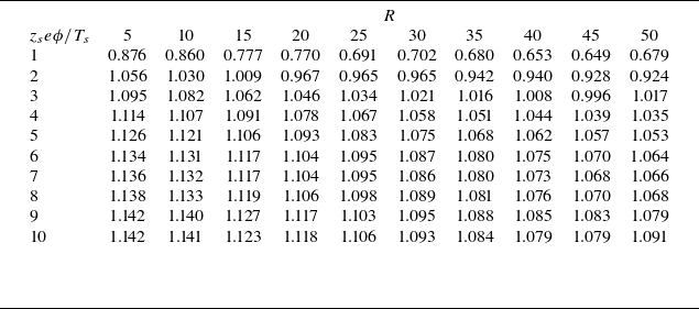


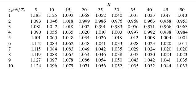


 Open access