


Impact Statement
Tree-ring chronologies encode essential information on how climate dynamics of the past have affected vegetation dynamics. Our proposed upscaling approach based on machine learning algorithms for regression can use sparse networks of tree-rings to reconstruct spatial patterns of climate-induced vegetation anomalies. We provide the first gridded data products of annual tree-ring indices across Europe that represent spatially resolved patterns of radial tree growth variability over more than 100 years. This data can be used for analyzing trends and extremes in vegetation growth, or linked to other data sources which might improve the understanding of atmosphere-biosphere interactions in the last century. Furthermore, our upscaling approach is very generic and can be applied to further regions, tree genera, and periods in time.
1. Introduction
Tree-ring data have been instrumental in the reconstruction of decadal to millennial climate history (Fritts, Reference Fritts1976; Jones et al., Reference Jones, Briffa, Osborn, Lough, van Ommen, Vinther and Xoplaki2009; St. George, Reference St. George2014; Esper et al., Reference Esper, Krusic, Ljungqvist, Luterbacher, Carrer, Cook and Büntgen2016; Wilson et al., Reference Wilson, Anchukaitis, Briffa, Büntgen, Cook, D’Arrigo and Zorita2016; Hartl-Meier et al., Reference Hartl-Meier, Büntgen, Smerdon, Zorita, Krusic, Ljungqvist and Esper2017a; Ljungqvist et al., Reference Ljungqvist, Piermattei, Seim, Krusic, Büntgen, He and Esper2020). However, considering the broad spatiotemporal dynamics they represent, we argue that tree-ring data are an underexploited resource in Earth system science. One reason is that tree-ring data often have no sufficient overlap with modern Earth observations, and another issue is that chronologies cannot be trivially updated (Babst et al., Reference Babst, Poulter, Bodesheim, Mahecha and Frank2017). Closing this gap of representation is of broad research interest because tree-rings can provide annually resolved information on forest growth variability over decades to millennia (Li et al., Reference Li, Nychka and Ammann2010; Babst et al., Reference Babst, Poulter, Bodesheim, Mahecha and Frank2017, Reference Babst, Bodesheim, Charney, Friend, Girardin, Klesse and Evans2018), a temporal domain unmatched by most other global observational resources of ecological dynamics and thereby of high relevance for, for example, evaluating terrestrial biosphere model dynamics (Rammig et al., Reference Rammig, Wiedermann, Donges, Babst, Von Bloh, Frank and Mahecha2015; Reference Barichivich, Peylin, Launois, Daux, Risi, Jeong and LuyssaertBarichivich et al., 2021; Reference Jeong, Barichivich, Peylin, Haverd, McGrath, Vuichard and LuyssaertJeong et al., 2021).
As systematic and repeated tree-ring sampling is impractical in many regions, we need to seek ways of estimating tree-ring growth where measurements are lacking. Progress has been made to simulate interannual tree-ring variability at the site level using different process-based modeling approaches or phenomenological models (Misson, Reference Misson2004; Breitenmoser et al., Reference Breitenmoser, Brönnimann and Frank2014; Li et al., Reference Li, Harrison, Prentice and Falster2014; Mina et al., Reference Mina, Martin-Benito, Bugmann and Cailleret2016). Yet, the current generation of mechanistic models suffers key structural deficits that often result in a poor representation of internal carbon storage dynamics and resource investment in woody biomass formation, such as radial tree growth (Fatichi et al., Reference Fatichi, Leuzinger and Körner2014, Reference Fatichi, Pappas, Zscheischler and Leuzinger2019; Zhang et al., Reference Zhang, Babst and Bellassen2018). In view of these limitations, an alternative to mechanistic modeling is the statistical upscaling of existing measurements based on observed relationships with key environmental variables (Babst et al., Reference Babst, Bodesheim, Charney, Friend, Girardin, Klesse and Evans2018). Machine learning techniques have been successfully applied for solving such problems (Jung et al., Reference Jung, Reichstein, Schwalm, Huntingford, Sitch, Ahlström and Zeng2017, Reference Jung, Koirala, Weber, Ichii, Gans, Camps-Valls and Reichstein2019, Reference Jung, Schwalm, Migliavacca, Walther, Camps-Valls, Koirala and Reichstein2020; Bodesheim et al., Reference Bodesheim, Jung, Gans, Mahecha and Reichstein2018) and here we are exploring their capacity to upscale tree-ring data across Europe.
Our approach is essentially the opposite of using tree-ring data to reconstruct the climate of the past: we use meteorological measurements as explanatory variables for reconstructing tree-ring growth variability at ungauged sites. When we talk about tree-ring growth variability, we essentially mean tree-ring indices in the way they are usually computed from site-level measurements of radial tree-ring widths, which is explained in detail in Section 2.1. By exploiting the power of data-driven nonlinear regression approaches as they are common now for machine learning, we are able to estimate tree-ring indices based on the inferred relationships to the climatic conditions obtained from site-level chronologies. A summary of our approach is shown in Figure 1. As a result, we provide gridded products of annual tree-ring variability that can easily be compared to remotely sensed Earth observations and mechanistic model estimates of forest dynamics. We explore different prediction strategies by varying the amount of climate information that is covered by the driver variables and compare the results of corresponding cross-validation experiments.
The outline of our approach for estimating tree-ring indices in order to produce gridded tree-ring data by exploiting machine learning methods for regression, in particular the Gaussian process (GP) framework and the random decision forest (RDF) approach.

Throughout our study, we aim at predicting at the genus level, since trees from different genera are expected to respond very differently to climate conditions. Due to the limited tree-ring data availability in our study region, we focus on the six most prominent genera in Europe: Abies (AB), Fagus (FA), Larix (LA), Picea (PC), Pinus (PI), and Quercus (QU). The datasets we are using in this study are described in the following section.
2. Data
Three different types of datasets are used in our study. Our target data is a compilation of available tree-ring data at site-level that give us very local information about relative growth rates of trees from different species. Note that tree-ring data is often not representative for the whole forest as people have often sampled the largest and oldest trees of a site (Nehrbass-Ahles et al., Reference Nehrbass-Ahles, Babst, Klesse, Nötzli, Bouriaud, Neukom and Frank2014; Babst et al., Reference Babst, Bodesheim, Charney, Friend, Girardin, Klesse and Evans2018). However, even if the tree-ring chronologies do not represent the whole forest, they are still the best estimates of tree-growth variability we can get so far with the available data and we therefore use them for our upscaling approach. One should nonetheless keep in mind that long-term growth trends are especially affected and sample biases can also influence the high-frequency signals in the tree-ring data.
As predictors we use climate data for explaining the variability in tree-ring growth with respect to both the spatial and the temporal domain. Hence, the climate data should be at a reasonable spatial scale as well as with a large temporal extent to maximize the overlap with available tree-ring data. We make use of two different climate datasets in order to cover both aspects. We describe both datasets in detail after introducing the tree-ring data in the following section.
2.1. Tree-ring data
For automatically learning the relationships between climate conditions and tree-ring growth, we use publicly available tree-ring index data from the International Tree-Ring Data Bank (ITRDB).Footnote 1 During preprocessing, the raw ring width data have been standardized using a cubic smoothing spline detrending with a 50% frequency cutoff response at 30 years. To achieve this, a spline was fit through the raw time series obtained from each individual sample at a given site. Growth variability was then calculated by dividing the measured ring width for a given year by the corresponding value from the smoothing spline. This resulted in a dimensionless index that retains interannual to multidecadal variability in tree growth, but removes longer-term trends. All detrended series from a given site were averaged into a site-level chronology using Tukey’s biweight robust mean. From a numerical point of view, each chronology is a time series at annual scale with values roughly between 0 and 3 and a mean value of 1 (see Figure 2a).
Overview of the tree-ring data used within this article. Samples of tree-ring chronologies are shown in (a) and the distribution of available time series among the different genera is depicted in (b). The spatial distribution of sites is plotted in (c–h).

For our study, we additionally use tree-ring data provided by Claudia Hartl and Christian Zang consisting of 245 chronologies (Abies: 72, Fagus: 52, Larix: 7, Picea: 87, Pinus: 8, Quercus: 19) from 143 sites in Central Europe (Hartl-Meier et al., Reference Hartl-Meier, Dittmar, Zang and Rothe2014a,Reference Hartl-Meier, Zang, Büntgen, Esper, Rothe, Göttlein and Treydteb,Reference Hartl-Meier, Zang, Dittmar, Esper, Göttlein and Rothec, Reference Hartl-Meier, Esper, Liebhold, Konter, Rothe and Büntgen2017b; Zang et al., Reference Zang, Hartl-Meier, Dittmar, Rothe and Menzel2014). The raw data underwent the same preprocessing as the ITRDB data, hence we were able to simply merge both datasets in order to get a broader view on tree-ring growth in Europe. The number of available time series for each genus in our dataset is shown in Figure 2b. Furthermore, Figure 2c–h shows the spatial distribution of the sites that yielded the chronologies of each genus.
2.2. Monthly climate data
As predictor variables, we use monthly statistics of climate observations (variable names are given in Table 1) from the Climate Research Unit Time Series (CRU TS) dataset (version 3.22) provided by Harris et al. (Reference Harris, Jones, Osborn and Lister2014). All predictor variables are available for the years 1901–2013 covering a large fraction of the tree-ring measurements that can be used to learn a machine learning model for estimating tree-ring indices from climate variables. Note that the data quality may be lower in the earliest portion of the CRU TS dataset, because the density of met stations grows thinner back in time. However, we do not expect major quality losses, because in Europe this problem is much less acute than in other regions of the world.
Variables of the CRU TS dataset (version 3.22) that have been used as predictor variables for estimating tree-ring indices.

To obtain the predictor variables for the individual sites where we have in situ measurements of tree-rings, the corresponding values have been extracted from the gridded products and the corresponding grid cells of each site. Because it is known that tree-ring growth for a single year does not only depend on the climate of this specific year but also of the previous year, we considered for each annual tree-ring measurement the monthly predictor values of the corresponding as well as its preceding year.
2.3. Static climate data
CRU TS data encode the temporal climate anomalies but information is only available at a rather coarse spatial resolution (half-degree). In order to understand whether the prediction of tree-ring indices benefits from a more detailed description of the individual site conditions, we additionally use monthly mean seasonal cycles of both climate data and bioclimatic variables at a spatial resolution of 1 km to incorporate general growth conditions at each site. These mean seasonal cycles are taken from the WorldClim dataset (version 2) provided by Fick and Hijmans (Reference Fick and Hijmans2017), where the monthly average values have been computed from the years 1970–2000. We use all seven climate variables listed in Table 2 and all 19 bioclimatic variables listed in Table 3.
Climate variables of the WorldClim dataset (version 2) that have been used as predictor variables for estimating tree-ring indices.
Bioclimatic variables of the WorldClim dataset (version 2) that have been used as predictor variables for estimating tree-ring indices.
3. Machine Learning Approaches for Regression
We tested two different and well-established machine learning approaches for regression. On the one hand, we selected the random decision forest (RDF) framework (Breiman, Reference Breiman2001), because this technique has been proven to be useful in other upscaling tasks such as the upscaling of land-atmosphere fluxes (Tramontana et al., Reference Tramontana, Jung, Schwalm, Ichii, Camps-Valls, Raduly and Papale2016; Bodesheim et al., Reference Bodesheim, Jung, Gans, Mahecha and Reichstein2018). On the other hand, we performed experiments with the Gaussian process (GP) framework (Rasmussen and Williams, Reference Rasmussen and Williams2006), because it is an elegant mathematical concept and offers more flexibility in learning the relationships between climate and tree growth while the computational costs do not reach the limits of current hardware in terms of memory and reasonable computation time due to the moderate size of the tree-ring dataset that we are using. In the following two subsections, we describe the basic ideas as well as the important properties of the two approaches.
For both of them, we assume a given training set $ \mathcal{X}\hskip3.00pt =\hskip3.00pt \{{\overrightarrow{x}}^{(i)}\hskip1.5pt \in \hskip1.5pt \mathrm{I}{\mathrm{R}}^D:i\hskip1.5pt =\hskip1.5pt 1,2,\dots, N\} $
of
$ \mathcal{X}\hskip3.00pt =\hskip3.00pt \{{\overrightarrow{x}}^{(i)}\hskip1.5pt \in \hskip1.5pt \mathrm{I}{\mathrm{R}}^D:i\hskip1.5pt =\hskip1.5pt 1,2,\dots, N\} $
of $ N $
samples with each sample
$ N $
samples with each sample $ \overrightarrow{x} $
being a vector consisting of
$ \overrightarrow{x} $
being a vector consisting of $ D $
predictor variables
$ D $
predictor variables $ {x}_1,{x}_2,\dots, {x}_D $
(e.g., climate variables) and a corresponding real-valued target variable
$ {x}_1,{x}_2,\dots, {x}_D $
(e.g., climate variables) and a corresponding real-valued target variable $ y\hskip1.5pt \in \hskip1.5pt \mathrm{IR} $
with observations
$ y\hskip1.5pt \in \hskip1.5pt \mathrm{IR} $
with observations $ {y}_1,{y}_2,\dots, {y}_N\hskip1.5pt \in \hskip1.5pt \mathrm{IR} $
, in our case the standardized tree-ring indices. The goal of training a machine learning model is to establish a relationship between
$ {y}_1,{y}_2,\dots, {y}_N\hskip1.5pt \in \hskip1.5pt \mathrm{IR} $
, in our case the standardized tree-ring indices. The goal of training a machine learning model is to establish a relationship between $ \overrightarrow{x} $
and
$ \overrightarrow{x} $
and $ y $
such that we are able to estimate an output (tree-ring index)
$ y $
such that we are able to estimate an output (tree-ring index) $ {y}^{\ast } $
for an unseen composition of predictor variables
$ {y}^{\ast } $
for an unseen composition of predictor variables $ {\overrightarrow{x}}^{\ast } $
.
$ {\overrightarrow{x}}^{\ast } $
.
It is important to note that both approaches are able to model the interactions of predictor variables implicitly without explicit specifications. This might especially be crucial for the interactions of temperature and precipitation to cope with the influence of droughts on tree growth.
3.1. Random decision forest
Random forest, also called RDF, is an ensemble method described by Breiman (Reference Breiman2001) that can be used for regression tasks. It consists of several individual regression models called random decision trees and each decision tree provides an estimate for the output. The number of decision trees is a parameter that needs to be specified prior to the learning step and the outputs of all the decision trees are averaged to obtain the predicted value for a test sample.
Learning a decision tree model consists of recursively splitting the training dataset into two subsets by a simple threshold function applied to a single predictor variable in $ \overrightarrow{x} $
. The threshold
$ \overrightarrow{x} $
. The threshold $ {t}_i $
and the selected predictor variable
$ {t}_i $
and the selected predictor variable $ {x}_{d_i} $
are optimized in each step
$ {x}_{d_i} $
are optimized in each step $ i $
, for example, by minimizing the root-mean-square error (RMSE) with respect to the current estimate that is given by the average observation
$ i $
, for example, by minimizing the root-mean-square error (RMSE) with respect to the current estimate that is given by the average observation $ \overline{y} $
of samples in the corresponding subset. Recursively splitting the training dataset in smaller subsets leads to a special graph structure in computer science: a binary tree. An example is shown in Figure 3. Since the subsets of data become smaller when the binary tree grows larger, the mean value of the observations becomes a better estimate. In order to avoid overfitting, splitting is not done until only one sample is left in each subset but until some stopping criterion is met, for example, minimum number of samples in a subset is reached or variance of observations within a subset is smaller than a predefined threshold.
$ \overline{y} $
of samples in the corresponding subset. Recursively splitting the training dataset in smaller subsets leads to a special graph structure in computer science: a binary tree. An example is shown in Figure 3. Since the subsets of data become smaller when the binary tree grows larger, the mean value of the observations becomes a better estimate. In order to avoid overfitting, splitting is not done until only one sample is left in each subset but until some stopping criterion is met, for example, minimum number of samples in a subset is reached or variance of observations within a subset is smaller than a predefined threshold.
A binary decision tree visualizing the concept used within RDFs for regression. Estimates for the target variable $ y $
are stored in the leaf nodes and the prediction for sample
$ y $
are stored in the leaf nodes and the prediction for sample $ \overrightarrow{x} $
is obtained from the leaf node that is reached by evaluating threshold functions applied to individual predictor variables. Similar to Bodesheim et al. (Reference Bodesheim, Jung, Gans, Mahecha and Reichstein2018), Figure 1.
$ \overrightarrow{x} $
is obtained from the leaf node that is reached by evaluating threshold functions applied to individual predictor variables. Similar to Bodesheim et al. (Reference Bodesheim, Jung, Gans, Mahecha and Reichstein2018), Figure 1.

The final binary tree structure then contains two types of nodes: (a) inner nodes that define a split by storing the index $ {d}_i $
of one of the
$ {d}_i $
of one of the $ D $
predictor variables and a corresponding threshold
$ D $
predictor variables and a corresponding threshold $ {t}_i $
and (b) leaf nodes that are not split up further but which provide an regression estimate
$ {t}_i $
and (b) leaf nodes that are not split up further but which provide an regression estimate $ {\overline{y}}_j $
via the average observation of the samples that belong to the subset of training data reaching this leaf node (Figure 3). When learning multiple decision tree models in an ensemble, it is important to incorporate different kinds of randomization such that different trees can learn different relationships between predictor variables and observations and to avoid overfitting. The first randomization takes place before learning the tree structures. For each tree to be learned, a random subset of the training data is sampled with replacement to obtain different portions of the training data for every tree. Together with the fusion scheme (averaging) of the outputs of all binary trees in the end, this is called bagging (Breiman, Reference Breiman2001). Furthermore, for a split node not all
$ {\overline{y}}_j $
via the average observation of the samples that belong to the subset of training data reaching this leaf node (Figure 3). When learning multiple decision tree models in an ensemble, it is important to incorporate different kinds of randomization such that different trees can learn different relationships between predictor variables and observations and to avoid overfitting. The first randomization takes place before learning the tree structures. For each tree to be learned, a random subset of the training data is sampled with replacement to obtain different portions of the training data for every tree. Together with the fusion scheme (averaging) of the outputs of all binary trees in the end, this is called bagging (Breiman, Reference Breiman2001). Furthermore, for a split node not all $ D $
predictor variables and all plausible thresholds are tested to find an optimal split. Instead, a random subset of the variables is analyzed together with randomly selected thresholds in the corresponding range of the variable. The influence of randomization in the ensemble of decision trees is very important to obtain reasonable estimation performance of the random forest regression model.
$ D $
predictor variables and all plausible thresholds are tested to find an optimal split. Instead, a random subset of the variables is analyzed together with randomly selected thresholds in the corresponding range of the variable. The influence of randomization in the ensemble of decision trees is very important to obtain reasonable estimation performance of the random forest regression model.
3.2. The GP framework
GP regression denotes a flexible nonparametric framework that is based on probability theory. The textbook of Rasmussen and Williams (Reference Rasmussen and Williams2006) provides a comprehensive introduction and we only describe the main aspects of the regression method briefly in the following. Note that GP regression is often also referred to as kriging, however, mostly in conjunction with two- or three-dimensional input spaces (Rasmussen and Williams, Reference Rasmussen and Williams2006). A GP is a stochastic process, that is, a distribution over latent functions $ f $
, that can be specified by a prior mean function
$ f $
, that can be specified by a prior mean function $ \mu \left(\cdot \right) $
and a covariance function
$ \mu \left(\cdot \right) $
and a covariance function $ \kappa \left(\cdot, \cdot \right) $
. Assuming that
$ \kappa \left(\cdot, \cdot \right) $
. Assuming that $ y $
depends on
$ y $
depends on $ \overrightarrow{x} $
and an unknown function
$ \overrightarrow{x} $
and an unknown function $ f $
as well as an additive noise
$ f $
as well as an additive noise $ \varepsilon $
:
$ \varepsilon $
:
 $$ y\hskip1.5pt =\hskip1.5pt f\left(\overrightarrow{x}\right)+\varepsilon, $$
the idea is to average over all possible functions $ f $
that are able to describe the relationship of predictor variables
$ f $
that are able to describe the relationship of predictor variables $ \overrightarrow{x} $
and targets
$ \overrightarrow{x} $
and targets $ y $
in a full Bayesian manner and to use the average function value called posterior mean for a specific
$ y $
in a full Bayesian manner and to use the average function value called posterior mean for a specific $ {\overrightarrow{x}}^{\ast } $
to obtain the regression value
$ {\overrightarrow{x}}^{\ast } $
to obtain the regression value $ {y}^{\ast } $
. Hence, it is sufficient to specify
$ {y}^{\ast } $
. Hence, it is sufficient to specify $ \mu \left(\cdot \right) $
and
$ \mu \left(\cdot \right) $
and $ \kappa \left(\cdot, \cdot \right) $
of the GP prior as well as the noise process
$ \kappa \left(\cdot, \cdot \right) $
of the GP prior as well as the noise process $ \varepsilon $
in order to use the GP regression framework.
$ \varepsilon $
in order to use the GP regression framework.
Without any prior knowledge about the data, it is common to use the zero-mean assumption, that is, $ \mu (\overrightarrow{x})\hskip1.5pt =\hskip1.5pt 0\hskip1.5pt \forall \hskip1.5pt \overrightarrow{x} $
. Since the tree-ring chronologies have a mean value of 1 due to preprocessing and their characteristic of being a relative tree growth measure (cf. Section 2.1), a prior mean
$ \mu (\overrightarrow{x})\hskip1.5pt =\hskip1.5pt 0\hskip1.5pt \forall \hskip1.5pt \overrightarrow{x} $
. Since the tree-ring chronologies have a mean value of 1 due to preprocessing and their characteristic of being a relative tree growth measure (cf. Section 2.1), a prior mean $ \mu (\overrightarrow{x})\hskip1.5pt =\hskip1.5pt 1\hskip1.5pt \forall \hskip1.5pt \overrightarrow{x} $
incorporates this additional knowledge about the data. From a technical point of view, using
$ \mu (\overrightarrow{x})\hskip1.5pt =\hskip1.5pt 1\hskip1.5pt \forall \hskip1.5pt \overrightarrow{x} $
incorporates this additional knowledge about the data. From a technical point of view, using $ \mu (\overrightarrow{x})\hskip1.5pt =\hskip1.5pt 1\hskip1.5pt \forall \hskip1.5pt \overrightarrow{x} $
is equivalent to a transformation of all target values
$ \mu (\overrightarrow{x})\hskip1.5pt =\hskip1.5pt 1\hskip1.5pt \forall \hskip1.5pt \overrightarrow{x} $
is equivalent to a transformation of all target values $ y $
by subtracting 1, then predicting the transformed value with a GP regression model, and finally adding 1 to the prediction again to obtain the regression estimate for the tree-ring index.
$ y $
by subtracting 1, then predicting the transformed value with a GP regression model, and finally adding 1 to the prediction again to obtain the regression estimate for the tree-ring index.
The covariance function $ \kappa \left(\cdot, \cdot \right) $
measures the similarity of two input vectors
$ \kappa \left(\cdot, \cdot \right) $
measures the similarity of two input vectors $ \overrightarrow{x} $
and
$ \overrightarrow{x} $
and $ \overrightarrow{x}^{\prime } $
. In machine learning,
$ \overrightarrow{x}^{\prime } $
. In machine learning, $ \kappa $
is often called a kernel function. There exists a large amount of different kernel functions for different applications depending on the properties of the input data
$ \kappa $
is often called a kernel function. There exists a large amount of different kernel functions for different applications depending on the properties of the input data $ \overrightarrow{x} $
. The most common kernel function is the Gaussian radial basis function kernel (Gaussian RBF kernel) also called squared exponential kernel (SE kernel) by Rasmussen and Williams (Reference Rasmussen and Williams2006):
$ \overrightarrow{x} $
. The most common kernel function is the Gaussian radial basis function kernel (Gaussian RBF kernel) also called squared exponential kernel (SE kernel) by Rasmussen and Williams (Reference Rasmussen and Williams2006):
 $$ {\kappa}_{\mathrm{SE}}\left(\overrightarrow{x},\overrightarrow{x}^{\prime}\right)\hskip1.5pt =\hskip1.5pt {\sigma}_f^2\exp \left(\frac{-{\left|\overrightarrow{x}-\overrightarrow{x}\prime \right|}_2^2}{2{\mathrm{\ell}}^2}\right)\hskip1em . $$
It depends on the squared Euclidean distance between $ \overrightarrow{x} $
and
$ \overrightarrow{x} $
and $ \overrightarrow{x}^{\prime } $
as well as on the hyperparameters
$ \overrightarrow{x}^{\prime } $
as well as on the hyperparameters $ {\sigma}_f^2 $
and
$ {\sigma}_f^2 $
and $ {\mathrm{\ell}}^2 $
. While the process variance
$ {\mathrm{\ell}}^2 $
. While the process variance $ {\sigma}_f^2 $
affects the scaling of function values, the length-scale parameter
$ {\sigma}_f^2 $
affects the scaling of function values, the length-scale parameter $ {\mathrm{\ell}}^2 $
determines the relevant scale of the input vectors
$ {\mathrm{\ell}}^2 $
determines the relevant scale of the input vectors $ \overrightarrow{x} $
and
$ \overrightarrow{x} $
and $ \overrightarrow{x}^{\prime } $
. Both parameters can either be fixed manually or optimized within the probabilistic framework by maximizing the likelihood of the training data.
$ \overrightarrow{x}^{\prime } $
. Both parameters can either be fixed manually or optimized within the probabilistic framework by maximizing the likelihood of the training data.
The noise term $ \varepsilon $
in equation (1) is usually modeled as white Gaussian noise
$ \varepsilon $
in equation (1) is usually modeled as white Gaussian noise $ \varepsilon \sim \mathcal{N}\left(0,{\sigma}_{\varepsilon}^2\right) $
with
$ \varepsilon \sim \mathcal{N}\left(0,{\sigma}_{\varepsilon}^2\right) $
with $ {\sigma}_{\varepsilon}^2 $
being a hyperparameter that is either fixed (e.g.,
$ {\sigma}_{\varepsilon}^2 $
being a hyperparameter that is either fixed (e.g., $ {\sigma}_{\varepsilon}^2\hskip1.5pt =\hskip1.5pt 0.01 $
) or also optimized via likelihood maximization. The advantage of the Gaussian noise assumption is that the estimated output value
$ {\sigma}_{\varepsilon}^2\hskip1.5pt =\hskip1.5pt 0.01 $
) or also optimized via likelihood maximization. The advantage of the Gaussian noise assumption is that the estimated output value $ {y}^{\ast } $
of an input vector
$ {y}^{\ast } $
of an input vector $ {\overrightarrow{x}}^{\ast } $
then also follows a Gaussian distribution:
$ {\overrightarrow{x}}^{\ast } $
then also follows a Gaussian distribution: $ {y}^{\ast}\sim \mathcal{N}\left({\mu}_{\ast },{\sigma}_{\ast}^2\right) $
and inference within the probabilistic GP regression framework is analytically tractable. In fact, there exist closed-form solutions for the moments
$ {y}^{\ast}\sim \mathcal{N}\left({\mu}_{\ast },{\sigma}_{\ast}^2\right) $
and inference within the probabilistic GP regression framework is analytically tractable. In fact, there exist closed-form solutions for the moments $ {\mu}_{\ast } $
and
$ {\mu}_{\ast } $
and $ {\sigma}_{\ast}^2 $
:
$ {\sigma}_{\ast}^2 $
:
 $$ {\mu}_{\ast}\hskip1.5pt =\hskip1.5pt {\overrightarrow{k}}_{\ast}^{\mathrm{T}}\boldsymbol{K}\overrightarrow{y}, $$
 $$ {\sigma}_{\ast}^2\hskip1.5pt =\hskip1.5pt {k}_{\ast \ast }+{\sigma}_{\varepsilon}^2-{\overrightarrow{k}}_{\ast}^{\mathrm{T}}\boldsymbol{K}{\overrightarrow{k}}_{\ast}\hskip1em . $$
The $ N\times N $
kernel matrix
$ N\times N $
kernel matrix $ \boldsymbol{K} $
contains the pairwise similarities of the
$ \boldsymbol{K} $
contains the pairwise similarities of the $ N $
training samples, the vector
$ N $
training samples, the vector $ {\overrightarrow{k}}_{\ast } $
consists of similarities between the test sample
$ {\overrightarrow{k}}_{\ast } $
consists of similarities between the test sample $ {\overrightarrow{x}}^{\ast } $
and the
$ {\overrightarrow{x}}^{\ast } $
and the $ N $
training samples, and
$ N $
training samples, and $ {k}_{\ast \ast}\hskip1.5pt =\hskip1.5pt \kappa ({\overrightarrow{x}}^{\ast },{\overrightarrow{x}}^{\ast }) $
is the so-called self-similarity of
$ {k}_{\ast \ast}\hskip1.5pt =\hskip1.5pt \kappa ({\overrightarrow{x}}^{\ast },{\overrightarrow{x}}^{\ast }) $
is the so-called self-similarity of $ {\overrightarrow{x}}^{\ast } $
. Furthermore, the vector
$ {\overrightarrow{x}}^{\ast } $
. Furthermore, the vector $ \overrightarrow{y} $
is a collection of the output values
$ \overrightarrow{y} $
is a collection of the output values $ y $
from the
$ y $
from the $ N $
training samples. While the predictive mean
$ N $
training samples. While the predictive mean $ {\mu}_{\ast } $
in equation (3) is the estimated regression output for a test sample
$ {\mu}_{\ast } $
in equation (3) is the estimated regression output for a test sample $ {\overrightarrow{x}}^{\ast } $
, the GP framework allows for quantifying the uncertainty of this estimate via the predictive variance
$ {\overrightarrow{x}}^{\ast } $
, the GP framework allows for quantifying the uncertainty of this estimate via the predictive variance $ {\sigma}_{\ast}^2 $
(equation (4)). A visualization of both predictive mean and predictive variance is given in Figure 4.
$ {\sigma}_{\ast}^2 $
(equation (4)). A visualization of both predictive mean and predictive variance is given in Figure 4.
Example of GP regression for one-dimensional inputs (single predictor variable). Blue crosses indicate training data, the red curve is the estimated posterior mean function that defines the output values $ {\mu}_{\ast } $
for the targets
$ {\mu}_{\ast } $
for the targets $ {y}^{\ast } $
, and the shaded regions in orange visualize the uncertainties of the predictions by plotting the standard deviation derived from the posterior variance
$ {y}^{\ast } $
, and the shaded regions in orange visualize the uncertainties of the predictions by plotting the standard deviation derived from the posterior variance $ {\sigma}_{\ast}^2 $
at each position
$ {\sigma}_{\ast}^2 $
at each position $ {x}^{\ast } $
in the predictor space.
$ {x}^{\ast } $
in the predictor space.

4. Experimental Setup and Results
In this section, we present the results we have obtained from our experiments. First, we motivate our strategy of explicitly distinguishing different genera of trees in Section 4.1. We then describe the basic setup of our experiments for assessing the prediction performances of the two analyzed machine learning methods for estimating tree-ring indices (Section 4.2). Afterwards in Sections 4.3–4.6, we discuss the individual findings and present the corresponding results. Further results are summarized in Appendix A.
4.1. Distinguishing different tree genera
We already mentioned in the introduction that we estimate tree-ring growth rates for different genera, because each genus responds differently to the same climate conditions. This can already be inferred from the tree-ring chronologies in the dataset that we are using. In particular, we identified 57 locations in our dataset where we have a tree-ring chronology for both beech trees (Fagus) and oak trees (Quercus). At each of these locations, the beech trees and the oak trees have encountered the same environmental conditions that are represented by the different climate variables. For each pair of chronologies, we computed the correlation coefficient taking only the years of the common time period into account. The distribution of the resulting correlation coefficients is shown as a histogram in Figure 5. Out of the 57 pairs of chronologies, 45 pairs obtain a value smaller than 0.45, which indicates no clear correlation and at most a rather weak connection. Hence, this small analysis supports our strategy of training regression models individually for each genus.
Distribution of correlation coefficients computed from pairs of chronologies consisting of one chronology for beech trees (Fagus) and one chronology for oak trees (Quercus) both sampled at the same site. This highlights the fact that trees from different genera respond different to the same climatic conditions.

4.2. Basic setup
We have learned individual regression models for each of the six most prominent genera in Europe, namely Abies (fir), Fagus (beech), Larix (larch), Picea (spruce), Pinus (pine), and Quercus (oak), with the distribution of chronologies among the genera depicted in Figure 2. For matching the tree-ring data with corresponding predictor variables that describe the environmental conditions, we only used the tree-ring indices corresponding to a year between 1901 and 2013 from each tree-ring chronology. Qualitative results are obtained using the predictions of a cross-validation scheme, more precisely a modified leave-one-site-out cross-validation for each genus. Leave-one-site-out means that for estimating the tree-ring growth rates at one site, regression models are learned using data from all the remaining sites that provide tree-ring data for the same genus. We have slightly modified this scheme by also excluding those sites from a training set, whose spatial coordinates fall into the same grid cell at half-degree resolution. This is due to the fact that our climate variables from the CRU TS dataset (Section 2.2) are at half-degree spatial resolution and we want to avoid different sites with probably different tree-ring chronologies having the exact same values for the predictor variables, which would lead to biased results. The modified leave-one-site-out is repeated such that data from each site is used in the test set once.
A quality criterion can be computed for each genus by comparing corresponding observations with predictions. In addition, an overall accuracy is provided by comparing observations and predictions across all genera. The quality measures that we have used to determine the performance of the different prediction approaches are the Nash–Sutcliffe model efficiency (Nash and Sutcliffe, Reference Nash and Sutcliffe1970), the RMSE, and Pearson correlation coefficient. In addition, we have computed the decompositions of the mean-square error (MSEs) following Gupta et al. (Reference Gupta, Kling, Yilmaz and Martinez2009) to obtain bias errors, variance errors, and phase errors. While bias errors denote an offset of individual predictions on average and variance errors indicate a different range of values for the predictions, phase errors for tree-ring chronologies at annual scale correspond to mismatches of the predicted interannual variability. Thus, phase errors indicate that peaks in the chronologies of observed and predicted values are not aligned or changes from reduced to increased tree-ring growth (change in tree-ring index from less than 1 to greater than 1) or vice versa happen in different years when comparing observations with predictions. For more details on these metrics in general, we refer to the original work (Gupta et al., Reference Gupta, Kling, Yilmaz and Martinez2009). When evaluating our different prediction approaches, we mainly focus on the model efficiency, which is similar to the coefficient of determination ( $ {R}^2 $
) and roughly summarizes the fraction of variance in the observations that can be explained by the predictions. The complete list of results regarding all six evaluation measures can be found in Appendix B.
$ {R}^2 $
) and roughly summarizes the fraction of variance in the observations that can be explained by the predictions. The complete list of results regarding all six evaluation measures can be found in Appendix B.
Our experiments are done in Matlab (version 2016b) using the TreeBagger function for RDF regression with its default parameter settings and specifying $ 100 $
decision trees in the ensemble. This means that the minimum node size, that is, the minimum number of samples in a leaf node, is set to five and for each split at an inner node, one third of all predictor variables are considered to find the best threshold. For GP regression, we have used the toolbox provided by Rasmussen and Nickisch (Reference Rasmussen and Nickisch2015). We have optimized the hyperparameters of the GP model (parameters of the kernel function as well as the noise variance) via likelihood maximization. It is important to note that a normalization of the predictor variables is required for the GP model in order to avoid numerical problems or instabilities (mainly when evaluating the kernel function and performing algebraic operations) and to allow for both robust learning and faster hyperparameter optimization. In all our experiments, we tried both: (a) normalization of predictor values to the interval
$ 100 $
decision trees in the ensemble. This means that the minimum node size, that is, the minimum number of samples in a leaf node, is set to five and for each split at an inner node, one third of all predictor variables are considered to find the best threshold. For GP regression, we have used the toolbox provided by Rasmussen and Nickisch (Reference Rasmussen and Nickisch2015). We have optimized the hyperparameters of the GP model (parameters of the kernel function as well as the noise variance) via likelihood maximization. It is important to note that a normalization of the predictor variables is required for the GP model in order to avoid numerical problems or instabilities (mainly when evaluating the kernel function and performing algebraic operations) and to allow for both robust learning and faster hyperparameter optimization. In all our experiments, we tried both: (a) normalization of predictor values to the interval $ \left[0,1\right] $
and (b) applying z-transformations such that the values of the individual predictor variables have zero mean and unit variance (following a standard normal distribution). Interestingly, there are hardly any differences in the prediction performance of the GP model with respect to the chosen normalization strategy. Throughout this article, we report results from our experiments when using the
$ \left[0,1\right] $
and (b) applying z-transformations such that the values of the individual predictor variables have zero mean and unit variance (following a standard normal distribution). Interestingly, there are hardly any differences in the prediction performance of the GP model with respect to the chosen normalization strategy. Throughout this article, we report results from our experiments when using the $ z $
-transformation
$ z $
-transformation $ \left(z,\hskip1.5pt ,=,\hskip1.5pt ,\frac{x-\mu }{\sigma}\right) $
for each individual predictor variable
$ \left(z,\hskip1.5pt ,=,\hskip1.5pt ,\frac{x-\mu }{\sigma}\right) $
for each individual predictor variable $ x $
with
$ x $
with $ \mu $
and
$ \mu $
and $ \sigma $
being the corresponding mean and standard deviation, respectively. Note that the performance of the RDF models are not affected by the normalization strategies, because the order of the values is preserved after the transformations and the RDF uses thresholds for splitting the data into subsets without any arithmetic calculations. Hence, normalization only changes the ranges for the randomized threshold selections during learning of the decision trees but there are no numerical issues that need to be considered.
$ \sigma $
being the corresponding mean and standard deviation, respectively. Note that the performance of the RDF models are not affected by the normalization strategies, because the order of the values is preserved after the transformations and the RDF uses thresholds for splitting the data into subsets without any arithmetic calculations. Hence, normalization only changes the ranges for the randomized threshold selections during learning of the decision trees but there are no numerical issues that need to be considered.
4.3. The impact of climate in the previous year
It is well-known in the field of dendrochronology that the width of tree-rings does not only depend on the environmental conditions during the corresponding year, but that growth is partially also responding to the climate conditions the tree had to cope with in the previous year (Fritts, Reference Fritts1976). Hence, our first hypothesis states that we gain additional information for the prediction of tree-ring indices by machine learning methods when we directly incorporate climate predictors from the year before each tree-ring was formed. This should then lead to improved prediction performance compared to regression models that only take the climate of the same year corresponding to the tree-ring into account.
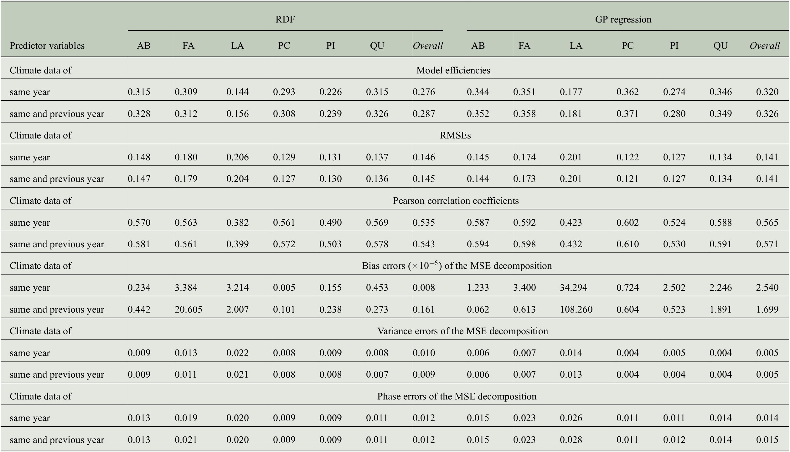
The results of our experiments are shown in Figure 6. It can be observed that for both regression models, RDF and GP, the modeling efficiencies in general slightly increase when taking the monthly climate predictors of the previous year into account. This holds for the overall results as well as for the predictions of individual genera and supports our initial hypothesis. Except for the RDF predictions of tree-ring indices for Fagus (model efficiency: 0.31) as well as GP predictions for Larix (model efficiency: 0.18) and Quercus (model efficiency: 0.35), a small improvement is visible. Although one might be tempted to say that these small improvements are not meaningful, it is important to mention again that the reported model efficiencies are computed from a set of leave-one-site-out experiments within each genus, hence for a large number of sites corresponding to each genus. The improvements are therefore achieved by models who have not seen the sites they predict and averaged over a whole genus.
Comparing the performance of RDF and GP models for predicting annual tree-ring indices for either considering only the monthly climate conditions of the same year (that corresponds to the tree-ring measurement) or for also taking the monthly climate of the previous year into account.

Furthermore, we observe that applying GP regression yields larger model efficiencies than the RDF models across all genera. In total, the best results are achieved by the GP regression approach with an overall model efficiency of 0.33 as well as the largest model efficiency for a single genus (0.37 for Picea). When considering the properties of model efficiency (optimal value is $ 1 $
and a value of 0 can already be obtained by simply predicting the overall mean value of the time series in each year), values between 0.3 and 0.4 seem to be quite low in general, since this corresponds to only 30–40% of explained variance. However, taking into account that methods for reconstructing climate in the past from tree-ring chronologies are often able to explain less than 50% of the signal variance at a single site (Esper et al., Reference Esper, Krusic, Ljungqvist, Luterbacher, Carrer, Cook and Büntgen2016) and our estimations of tree-ring indices from climate data (the other way around) tackle a much harder task by generalizing from a subset of sites to a different location (leave-one-site-out cross-validation), these initial results are quite promising. Note that the FLUXCOM studies (Jung et al., Reference Jung, Koirala, Weber, Ichii, Gans, Camps-Valls and Reichstein2019, Reference Jung, Schwalm, Migliavacca, Walther, Camps-Valls, Koirala and Reichstein2020) also report similar quality levels for their upscaling when considering annual integrals of the estimated carbon and energy fluxes because predicting interannual variability is a hard task in general. These studies consider two carbon fluxes, namely gross primary production (GPP) and net ecosystem exchange (NEE), and three energy fluxes (net radiation, sensible heat, and latent heat flux), while we report results for upscaling tree-ring indices.
$ 1 $
and a value of 0 can already be obtained by simply predicting the overall mean value of the time series in each year), values between 0.3 and 0.4 seem to be quite low in general, since this corresponds to only 30–40% of explained variance. However, taking into account that methods for reconstructing climate in the past from tree-ring chronologies are often able to explain less than 50% of the signal variance at a single site (Esper et al., Reference Esper, Krusic, Ljungqvist, Luterbacher, Carrer, Cook and Büntgen2016) and our estimations of tree-ring indices from climate data (the other way around) tackle a much harder task by generalizing from a subset of sites to a different location (leave-one-site-out cross-validation), these initial results are quite promising. Note that the FLUXCOM studies (Jung et al., Reference Jung, Koirala, Weber, Ichii, Gans, Camps-Valls and Reichstein2019, Reference Jung, Schwalm, Migliavacca, Walther, Camps-Valls, Koirala and Reichstein2020) also report similar quality levels for their upscaling when considering annual integrals of the estimated carbon and energy fluxes because predicting interannual variability is a hard task in general. These studies consider two carbon fluxes, namely gross primary production (GPP) and net ecosystem exchange (NEE), and three energy fluxes (net radiation, sensible heat, and latent heat flux), while we report results for upscaling tree-ring indices.
In our experiments, it is also interesting to observe that when comparing the results of the different tree genera, model efficiencies for Larix are notably smaller. On the one hand, the tree-ring dataset provides the smallest number of samples for Larix (see Figure 2) such that it is more difficult for a machine learning model to identify the relationship between predictor variables (climate) and the target variable (tree-ring index) due to the limited amount of example data. On the other hand, there is evidence that Larix in Europe is more sensitive to biological impacts. For instance, the larch budmoth is a widespread defoliator that feeds off fresh larch needles and periodically reaches outbreak levels (Esper et al., Reference Esper, Büntgen, Frank, Nievergelt and Liebhold2007; Hartl-Meier et al., Reference Hartl-Meier, Esper, Liebhold, Konter, Rothe and Büntgen2017b). These events are demarcated in the wood and partly obscure the obtained relationships between radial tree growth and climate. Since the influence of the larch budmoth complex population dynamics is not encoded in the predictor variables, important information is missing in the prediction models. The lower model efficiencies for larch trees can be observed in all our other experimental results that follow in the next sections but we will not repeat the previous explanations there.
Besides the model efficiencies, we also look at further evaluation measures mentioned in the previous section and the results are summarized in Table 4. The RMSE is largest for Larix with about 0.20 followed by Fagus with 0.17 to 0.18. The smallest RMSE is obtained for Picea with less than 0.13 and overall, the RMSE across all genera is between 0.14 and 0.15. While the RMSE for Fagus deviates more from the errors for other genera as well as from the overall values, the Pearson correlation for Fagus is similar to the overall correlation and to the one obtained for Abies, Picea, and Quercus. This is especially interesting when comparing the results for Fagus and Picea: Pearson correlation is almost the same whereas RMSE is clearly different. Hence, it is important to look at different evaluation measures.
Comparing the performance of RDF and GP models for predicting annual tree-ring indices with respect to six evaluation measures when taking monthly climate data from 1 or 2 years into account.
Abbreviations: GP, Gaussian process; MSE, mean-square error; RDF, random decision forest; RMSE, root-mean-square error.
We also computed error terms obtained from the decomposition of the MSEs (Gupta et al., Reference Gupta, Kling, Yilmaz and Martinez2009) and results are also summarized in Table 4. Note that for the bias errors, we report values that need to be scaled by a factor of $ {10}^{-6} $
. Therefore, we observe that all bias errors are smaller than
$ {10}^{-6} $
. Therefore, we observe that all bias errors are smaller than $ {10}^{-3} $
, which shows that there is no bias in any of the predictions, and the errors are distributed among the variance errors and the phase errors. For the predictions of the RDF models, we see that variance errors and phase errors are almost the same for three of the six genera (Larix, Picea, Pinus) and overall, both errors are roughly 0.01. Hence, for RDF models, the MSE is distributed rather equally among variance error and phase error. This is in contrast to the predictions of the GP models, where the phase error is two to three times larger than the variance error for each individual genus. Since variance errors for the GP models are lower than for the RDF models, we conclude that the GP models capture the variability in the tree-rings slightly better and have more problems in getting the phase, here the interannual variability, correctly.
$ {10}^{-3} $
, which shows that there is no bias in any of the predictions, and the errors are distributed among the variance errors and the phase errors. For the predictions of the RDF models, we see that variance errors and phase errors are almost the same for three of the six genera (Larix, Picea, Pinus) and overall, both errors are roughly 0.01. Hence, for RDF models, the MSE is distributed rather equally among variance error and phase error. This is in contrast to the predictions of the GP models, where the phase error is two to three times larger than the variance error for each individual genus. Since variance errors for the GP models are lower than for the RDF models, we conclude that the GP models capture the variability in the tree-rings slightly better and have more problems in getting the phase, here the interannual variability, correctly.
4.4. Climate predictors: Monthly versus seasonal scale
Given the fact that we use quite a large number of predictor variables due to the monthly time scale for the same and the previous year (2 years times 12 months times 10 climate variables = 240 predictor variables), we want to find out how prediction performance for tree-rings changes when we move from a monthly to a seasonal time scale for the predictor variables. Hence, we averaged the monthly values within seven seasons of the 2 years (MAM, JJA, SON, DJF, MAM, JJA, SON) to obtain 70 predictor variables (7 seasons times 10 climate variables) and performed the experiments with the aggregated data.
As it can be observed from Figure 7, the prediction performances in terms of model efficiency drop clearly for each genus. Comparing the two regression approaches, the reduction is larger for RDF regression (overall: from 0.29 to 0.22) compared to GP regression (overall: from 0.33 to 0.29). Thus, some important information for the prediction is lost when first computing seasonal means instead of using the monthly values directly. We conclude that in order to achieve better prediction performance, monthly climate data should be used rather than seasonal climate aggregations for estimating tree-ring indices.
Comparing the performance of RDF and GP models for predicting annual tree-ring indices regarding a monthly and a seasonal time scale of the predictor variables.

4.5. Taking monthly climate anomalies into account
Since tree-ring indices are relative growth values due to their dependency on an estimated trend that takes aging effects into consideration (see Section 2.1), they mainly represent deviations from an expected growing process and hence encode anomalies. This observation has brought us to another hypothesis that the climate conditions do not have a direct influence on the tree-ring growth rates but rather the climate anomalies, that is, the deviations from the average climate conditions at each site. We therefore performed experiments with anomalies of the climate predictors by subtracting the mean seasonal cycles that has been obtained by averaging over the years 1901–2000. The comparison of results from both settings, using anomalies or using the plain values, is shown in Figure 8.
Comparing the performance of RDF and GP models for predicting annual tree-ring indices by using either plain values of the climate variables or climate anomalies.

It can be clearly observed that our approach for predicting tree-ring growth rates benefits from the information that is encoded in the climate anomalies. Especially for RDF regression, substantial improvements can be observed. In this case, the overall performance increases from a model efficiency of 0.29 to a value of 0.34. While the GP regression models benefit less from the climate anomalies (but slight improvements are still visible), the largest increases in model efficiency occur for larch trees (Larix), the most difficult genus due to the small amount of available samples and the problems described in Section 4.3.
It is interesting to see that when using climate anomalies as predictors, the RDF regression approach is able to close the gap in performance that has been observed in the previous experiments, where GP regression achieved superior model efficiencies. By using the climate anomalies, both regression approaches are able to achieve an overall model efficiency of 0.34 for predicting tree-ring indices. At the genus level, both RDF and GP regression achieve a model efficiencies of 0.37 for Abies and Fagus as well as a model efficiency of 0.35 for Quercus. The model efficiencies for Picea are on the same level but slightly vary between both methods (RDF: 0.36, GP: 0.37), whereas the performance is worse for the remaining to genera (Larix and Pinus) considered in our studies.
In addition, we tested whether additional information is contained in the climate anomalies compared to the plain values of the climate variables. We therefore performed experiments with a set of predictor variables containing both the plain values and the anomalies of the climate variables and compared the results to the best ones achieved so far, that is, only using the climate anomalies. The corresponding model efficiencies are reported in Figure 9 and there are hardly any differences between the performance measurements, neither overall (model efficiency of 0.34 for both sets of predictor variables and both regression approaches) nor at a genus level (same values for Abies and Quercus, minor variations for the remaining four genera). Hence, we can conclude that all important information for predicting tree-ring indices from climate conditions is contained in the climate anomalies.
Comparison of the performances obtained with RDF and GP models for predicting annual tree-ring indices concerning the amount of information within the plain values and the anomalies of the climate predictor variables.

4.6. Incorporating static WorldClim data
So far, we have included climate conditions at a coarse spatial scale as predictor variables in our regression approaches. However, tree growth also depends on site-specific topographic characteristics that change much faster for different locations on much smaller spatial scales. To address this issue, we further use mean seasonal cycles of high-resolution climatic and bioclimatic variables from the WorldClim dataset as mentioned in Section 2.3. Note that these predictor variables are static and do not change over time. Hence, they cannot be used alone for estimating tree-ring growth rates in different years without any other predictors. However, they offer a way to incorporate site-specific topographic characteristics at high spatial resolution because they represent average conditions at each location and can thus be used in addition to time-varying climate predictor variables obtained from data products at coarser spatial scales.
From an ecological perspective, it is important to consider both types of variables together (high-resolution static climate data and low-resolution time-varying climate predictors), because a given climate anomaly, for example, a temperature increase of two degrees, has a different impact at different sites depending on the specific environmental conditions. On the one hand, if the baseline temperature is low and the growing season short, a two degree temperature increase will have a big impact on the tree growth rate. On the other hand, if the baseline temperature is high and the growing season long, the same climate anomaly will not have the same positive impact because the trees are already closer to a temperature optimum. It can even have a negative impact because water demand rises. By adding the static WorldClim data, we incorporate the baseline climate information such that the same climate anomalies can have a different impact on the tree growth rates.
Furthermore, local adaptations of trees might influence responses to climate anomalies as well, depending on what the trees are used to. However, we are missing corresponding data containing more detailed site-specific information, for example, for rooting depth, soil characteristics, as well as for properties of the stand, like density, age structure, and composition. Although this kind of data would be important to analyze forest adaptation and stand dynamics even better, it is not possible to incorporate factors like this for the predictions of the tree-ring indices given the available data. Another idea for modeling local adaptations would be to take the distance of a site to the edge of the species distribution range into account, but this is not straightforward and therefore left for future work. In this article, we only consider the static WorldClim data.
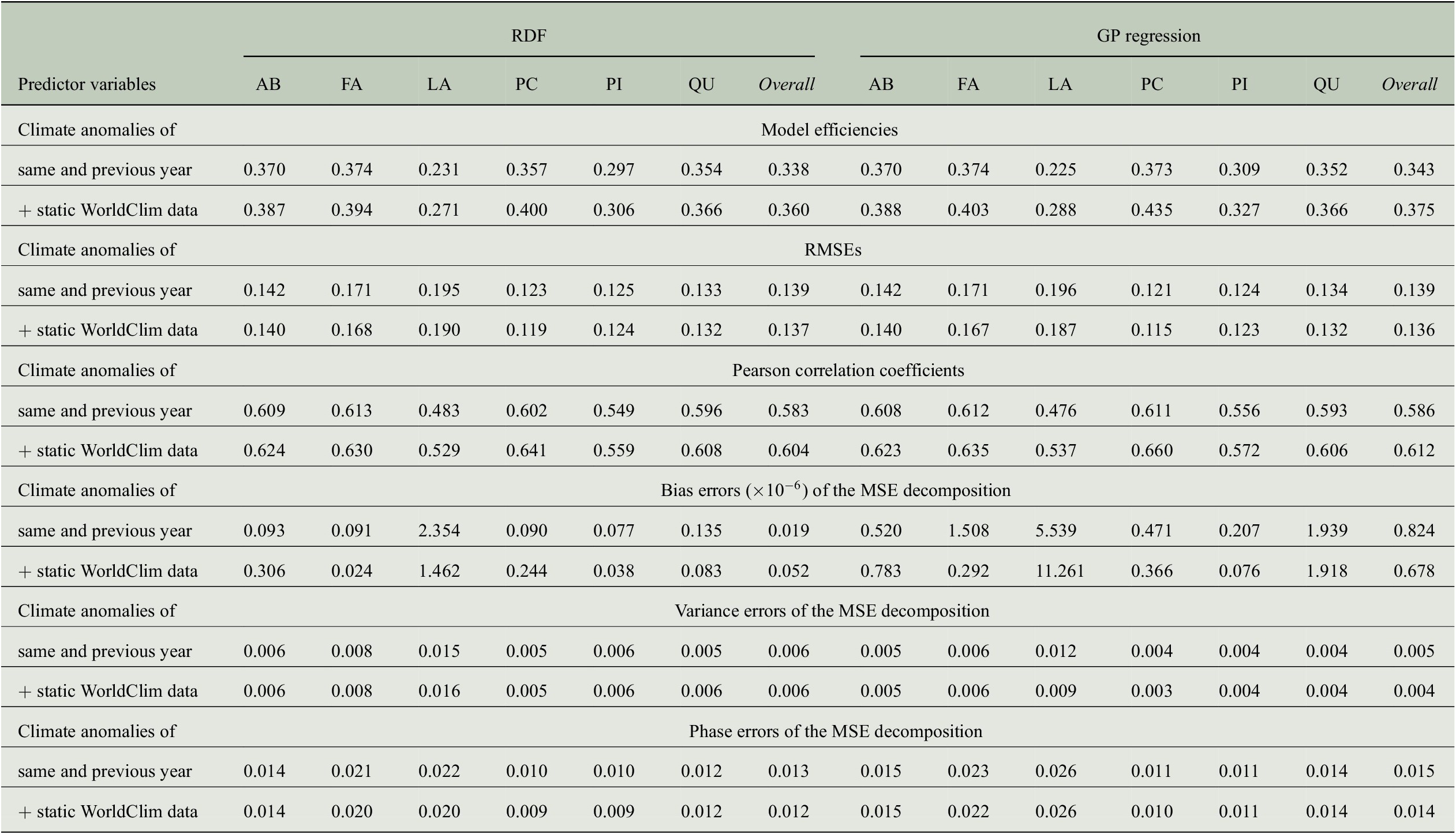
In Figure 10, we compare the previous best results using climate anomalies of the previous and same year as predictor variables with the setup in which we additionally use the static predictor variables from the WorldClim dataset, that is, the mean seasonal cycles of all variables from this dataset. The results clearly reveal the impact and the importance of high-resolution and site-specific topographic properties, because obtained modeling efficiencies are improved for each genus as well as overall by quite some margin when incorporating the WorldClim data. For the GP regression approach, the overall prediction performance in terms of modeling efficiency increases from 0.34 to 0.38 and for the RDF regression approach, an improvement from 0.34 to 0.36 can be observed. Looking at individual genera, largest improvements have been made for Larix (from 0.23 to 0.29) and Picea (from 0.37 to 0.44), which is very likely due to the fact that these are the genera with the strongest elevation gradient in the dataset.
Comparison of the performances obtained with RDF and GP models for predicting annual tree-ring indices with respect to the impact of high-resolution static data from the WorldClim dataset.

For more detailed investigations, we also show scatter plots of the predictions from the different regression models in Figure 11. It can be observed that the variance in the predictions of the GP models is slightly larger than in the predictions of the RDF models. This holds for all genera and is also reflected by the corresponding small differences in the modeling efficiencies. The variance in the observations is clearly larger for all genera compared to the variances in the predictions. Note that the scatter plots for the predictions from the previous experiments using other sets of predictor variables look quite similar and we therefore only include these plots here for giving more insights in the results with the best predictions.
Scatter plots for the predictions obtained with RDF models (a–f) and GP models (g–l) when using high-resolution static data from the WorldClim dataset in addition to the monthly climate anomalies of the CRU TS dataset.

The positive impact of the high-resolution static predictor variables can also be observed when looking at further evaluation measures summarized in Table 5. While the RMSE is only slightly reduced for all genera, Pearson correlation increases clearly. For the overall predictions of both regression approaches, the correlation coefficients exceed a value of 0.6 when using static WorldClim data as additional predictors. The bias errors of the MSE decompositions are all smaller than $ {10}^{-3} $
, that is, there is no bias in the predictions. Note that this is the case for the results of all our experiments, as shown in Table B4. In contrast to the results from Section 4.3, where the ratio of variance errors and phase errors was different for RDF predictions and GP predictions, we now see for both regression approaches that the largest amount of the MSE comes from the phase error, whereas the variance errors are clearly smaller. Concerning the overall predictions, the variance errors are between 0.004 and 0.006, while the phase errors are between 0.012 and 0.015. Although both errors hardly vary between the different sets of predictor variables (because also RMSE and hence MSE only differ slightly), model efficiencies and correlation coefficients are larger when taking the WorldClim data into account.
$ {10}^{-3} $
, that is, there is no bias in the predictions. Note that this is the case for the results of all our experiments, as shown in Table B4. In contrast to the results from Section 4.3, where the ratio of variance errors and phase errors was different for RDF predictions and GP predictions, we now see for both regression approaches that the largest amount of the MSE comes from the phase error, whereas the variance errors are clearly smaller. Concerning the overall predictions, the variance errors are between 0.004 and 0.006, while the phase errors are between 0.012 and 0.015. Although both errors hardly vary between the different sets of predictor variables (because also RMSE and hence MSE only differ slightly), model efficiencies and correlation coefficients are larger when taking the WorldClim data into account.
Comparing the performance of RDF and GP models for predicting annual tree-ring indices with respect to six evaluation measures when either only considering monthly climate anomalies as predictor variables or also taking static WorldClim data into account.
Abbreviations: GP, Gaussian process; MSE, mean-square error; RDF, random decision forest; RMSE, root-mean-square error.
Hence, we conclude that incorporating static predictor variables of high spatial resolution leads to clear performance boosts when estimating tree-ring growth rates and chronologies at unseen sites. As a next step, we perform an upscaling of site-level chronologies to gridded data products that are presented in the next section.
5. Gridded Tree-Ring Data Products for Europe
Encouragingly, with our machine learning approaches we are able to obtain spatialized and yearly resolved tree-ring indices. From the chronologies of in situ measurements at individual sites, we have learned regression models for each genus using all available chronologies of trees from the corresponding genus. We have computed dense products at two different spatial resolutions. For the coarser data products with 0.5° spatial resolution, we only used the time-varying predictor variables as done in our cross-validation experiments, that is, climate anomalies of the previous and the same year as in Section 4.5, which are extracted for each spatial grid cell in Europe. We also provide high-resolution data products at 0.0083° spatial resolution (roughly 1 km2), where we follow the approach of the previous section and use mean seasonal cycles of the variables from the WorldClim dataset as additional predictors beside the time-varying predictors that are extracted from the corresponding grid cells of the CRU TS dataset. The produced data products are available at https://www.doi.org/10.17871/BACI.248 (Bodesheim et al., Reference Bodesheim, Babst, Frank, Zang, Jung, Reichstein and Mahecha2021) and cover the years 1902–2013.
Note that the data products at both spatial resolutions differ in the way they have been calculated and one product is not simply the spatial aggregation of the other one. This is also discussed in Section 5.1 and shown in Figure 14. For the product at 0.5° spatial resolution, we restricted the set of predictor variables to the time-varying ones such that the resolution of the predictor variables matches the resolution of the obtained data product. For the product at 0.0083° spatial resolution, we additionally incorporated static data in terms of mean seasonal cycles of variables from the WorldClim dataset as additional predictor variables. Although this higher spatial resolution then only comes from static predictor variables that do not change over time, they are used in combination with the time-varying predictors when estimating the tree-ring indices in each year. Hence, for each individual prediction at a single grid cell, a different set of values for the predictor variables is used compared to the other grid cells. Thus, when considering the high-resolution grid cells that belong to a single grid cell at 0.5° spatial resolution, the patterns that are induced by values estimated for the high-resolution grid cells may vary across different years.
For both spatial resolutions, we also used both the RDF regression approach and the GP regression approach to perform the upscaling task. Regarding the hyperparameters of the individual methods, we used the same values as for the cross-validation experiments discussed in the previous sections. Based on the regression models for each genus as well as the predictor variables for each grid cell and each year, spatialized tree-ring indices can be estimated.
Of course, it only makes sense to predict tree-ring indices for grid cells where the trees of the corresponding genus occur. Therefore, we made use of the tree species distribution maps from the European Atlas of Forest Tree Species (de Rigo et al., Reference de Rigo, Caudullo, Houston Durrant and San-Miguel-Ayanz2016) containing relative probabilities of presence. The high-resolution data with grid cell sizes of 1 km2 has been used to decide whether we predict the tree-ring index at each spatial location. For our data product at 0.0083° spatial resolution, we could directly match the species distribution information and estimated tree-ring indices for those grid cells that have a value larger than 5% in the species distributing maps, that is, an occurrence probability higher than 5%. Since our estimated tree-ring indices are on the genus level, we consider each grid cell in which the presence of at least one corresponding species is at least 5%. For our data product at 0.5° spatial resolution, we need to aggregate the information from the species distribution maps. In particular, we have treated the large grid cell as a valid one for a genus if at least in one smaller grid cell of corresponding species distribution maps, the presence of the trees is at least 5%. Thus, we could restrict our estimations to a smaller set of grid cells compared to whole Europe.
At this point, we already want to add a cautious note regarding the interpretation and usage of our data products. As indicated above, our regression models are learned with data from sites whose locations are shown in Figure 2. For some genera, for example, Fagus, the utilized network of sites does not span the whole continent, but we, nevertheless, predict tree-ring indices across whole Europe. Hence, there might be some extrapolation involved in the predictions, in particular for regions with climate conditions that are potentially not observed during training of the model. We therefore encourage to always consider the spatial locations of the sites used during model training shown in Figure 2 as well when interpreting our data products or when drawing further conclusions that probably also arise in future studies. Although this might look like a limitation for our approach and our provided data products, it is still the best we can do so far with the limited availability of tree-ring data. We believe that our data products are nevertheless a valuable source for future research and we want to highlight again that results need to be interpreted with caution.
5.1. Example maps at two spatial resolutions
To illustrate our computed data products, some example maps are provided in Figure 12. We have selected two genera (Fagus and Quercus) and show corresponding maps at 0.5° spatial resolution for the (randomly selected) years 1980, 1990, and 2000, respectively. One can observe from these maps that trees of different genera respond differently to the same climate conditions when comparing maps of the same year, for example, looking at the same regions in both the map for Fagus of the year 2000 and the map for Quercus of the year 2000. Thus, it is important to make appropriate distinctions on the genus or species level. We also verified this observation based on the chronologies from the in situ measurements (Section 4.1 and Figure 5).
Estimated tree-ring indices of Fagus (a–c) and Quercus (d–f) at 0.5° spatial resolution in Europe from the RDF regression approach are visualized for the years 1980, 1990, and 2000, respectively.

In Figure 13, we display maps corresponding to the year 1990 at the two different spatial resolutions (0.5° and 0.0083°). We have selected the estimations for Fagus from the RDF regression approach as well as the estimations for Quercus from the GP regression approach. In both cases, we observe that the same patterns are obtained when comparing predictions at different spatial resolutions, for example, the green regions in the maps for Fagus and Quercus as well as the dark red area in the maps for Fagus.
Comparing the data products of the different spatial resolutions 0.5° (a,c) and 0.0083° (b,d) by the corresponding maps of the year 1990 for the RDF regression approach and Fagus (a,b) as well as for the GP regression approach and Quercus (c,d).

To show the differences of the predictions that are achieved for the different resolutions, we compute spatially aggregated maps by calculating average values from corresponding grid cells of the high-resolution product (0.0083°) to match the lower resolution (0.5°). We are then able to determine the difference maps between the data products at 0.5° spatial resolution and the spatial aggregations of the data products at 0.0083° spatial resolution. These difference maps are shown in Figure 14 for the same examples as in Figure 13. In total, differences are rather small, since the same patterns are found in both versions of the tree-ring maps. Interestingly, the absolute differences in the maps for Fagus are largest in Western Europe (larger negative differences) and South Eastern Europe (larger positive differences), while absolute differences in the maps for Quercus are largest in Central Europe (larger negative differences).
Comparing the differences between the data product at 0.5° spatial resolution and spatial aggregations of the high-resolution product (0d0083@0d50) using the corresponding maps of the year 1990 for the RDF regression approach and Fagus (a–d) as well as for the GP regression approach and Quercus (e–h).

From the distributions of differences in Figure 14, we observe that a different resolution for the prediction does not lead to a bias in the estimated values. The variance of the differences is larger for Fagus than for Quercus, which can be explained by the larger variability of tree-ring indices for Fagus. For the maps of Quercus, there is hardly any difference between the predictions at 0.5° spatial resolution and the aggregated predictions at 0.0083° spatial resolution.
5.2. Differences in estimations of different regression approaches
In this section, we compare the estimations of the two regression approaches using the gridded data products at 0.5° spatial resolution. Difference maps of selected years are found in Figure 15 for predicted tree-ring indices of Fagus and in Figure 16 for predicted tree-ring indices of Quercus.
Comparing the differences between the predictions from the RDF approach and the GP approach for the estimated tree-ring indices of Fagus at 0.5° spatial resolution in the years 1980 (a–d), 1990 (e–h), and 2000 (i–l), respectively.

Comparing the differences between the predictions from the RDF approach and the GP approach for the estimated tree-ring indices of Quercus at 0.5° spatial resolution in the years 1980 (a–d), 1990 (e–h), and 2000 (i–l), respectively.

Considering the predictions for Fagus in Figure 15, we observe that the GP approach produces larger values for tree-ring growth in 1980 in Central Europe due to the red region in the difference map, where both regression approaches estimate a large increase in tree growth indicated by the green color in the original tree-ring maps. For the years 1990 and 2000, largest differences are observed in Western Europe and Eastern Europe. However, both regression approaches produce the same patterns for all the years, that is, red regions for reduced tree-ring growth and green regions for increased tree-ring growth match quite well. This can also be observed for the tree-ring predictions of Quercus in Figure 16.
When looking at the distributions of differences in Figure 16, we see that there is no bias when comparing the predictions of the RDF and the GP models for Quercus, since the distributions are symmetric and centered around zero. Interestingly, this is not the case for the distributions of differences in the predictions when considering tree-rings of Fagus. In Figure 15, the distributions are skewed and shifted by an offset that can be either positive or negative. Hence, there is no consistent bias meaning that for some years, RDF produces larger values than GP and for some years, it is vice versa. However, the absolute differences in the predictions are overall rather small compared to the variability of the estimated tree-ring indices (less than 0.2) and the produced spatial patterns are still the same for both regression approaches. The different behavior when comparing Fagus and Quercus might come from the different variability in the tree-ring indices for the different genera, which is also visualized in Figure 11. Hence, the two regression approaches handle the varying amount of variability in the target variable differently.
5.3. Tree-ring maps for selected years with extreme climate conditions
To further highlight the benefits of our upscaling approach and the derived data products, we explore tree growth patterns for years with extreme climate conditions. The years 1976 and 2003 are known to be very hot and dry ones (Rammig et al., Reference Rammig, Wiedermann, Donges, Babst, Von Bloh, Frank and Mahecha2015; Zhang et al., Reference Zhang, Babst and Bellassen2018). We further selected extreme years by considering monthly temperature and precipitation values from the CRU TS dataset. In particular, mean temperature and total precipitation aggregated over the 12 months have further been averaged spatially across the whole continent to obtain an average temperature and an average precipitation for each year. After sorting the years according to these two values, we have identified two hot and wet years (1999 and 2002), two cold and wet years (1940 and 1965), and two cold and dry years (1908 and 1942). Corresponding maps for Fagus and Quercus obtained by the two different regression approaches are shown in Figure 17. Note that these extreme conditions have been determined by taking average values across the whole continent into account. Hence, tree-ring indices might vary a lot when comparing local regions with probably larger deviations from the average climate conditions.
Predicted tree-ring maps of Fagus and Quercus at 0.5° spatial resolution from RDF models and GP models for years with extreme climate conditions: 2003 and 1976 as two hot and dry years (a–d), 2002 and 1999 as two hot and wet years (e–h), 1965 and 1940 as two cold and wet years (i–l), as well as 1942 and 1908 as two cold and dry years (m–p).

Nevertheless, it is interesting to see how different tree genera respond differently to extreme climate conditions. From Figure 17, we observe that beech and oak trees suffered a lot from heat and dryness in 1976 because the maps show many red and orange pixels indicating tree-ring indices smaller than one. Interestingly, similar conditions have been less detrimental for the trees in 2003, where mainly regions in Eastern Europe show reduced growth rates. One reason might be that tree growth is also influenced by the climate conditions of the previous year and 2002 has been one of the years with largest average precipitation. While also during hot years, tree growth in 2002 as well as in 1999 is less affected by the high temperatures due to higher water availability caused by more precipitation. In 1999, larger green areas can be observed in the map for Fagus, which is an indicator for increased growth rates with tree-ring indices larger than one. For the two cold and wet years 1940 and 1965, it can be observed that reduced tree growth especially happened in the very cold year 1940 for both Fagus and Quercus. During the two cold and dry years 1942 and 1908, we see that tree growth for oak trees was more inhibited compared to the growth of beech trees, which suffered more from the conditions in the very cold year 1942.
Last but not least, we want to look at tree-ring indices for the three consecutive years 2002, 2003, and 2004, which are all hot years. The associated maps for Fagus and Quercus are shown in Figure 18. As mentioned before, 2002 was a very wet year and hence, also large tree-ring indices greater than one appear in a region in Central Europe, whereas the tree growth is negatively affected in Southern Europe. In the following extreme year 2003, there is still one larger green region visible in the maps for Fagus, despite the very hot and dry conditions during this year. However, one year later in 2004, this green region turned into a red one, which indicates that the impact of the extremely hot and dry year 2003 is stronger for the tree growth in the following year 2004. This nicely highlights the lag effect of the climate conditions on tree growth. Furthermore, the effects of climate anomalies on tree growth also depend much on the time when the anomalies happen during a year. For example, a hot and dry event during (late) summer might have less severe consequences for the tree growth in the same year if large amounts of the tree-ring have been built already during the months before with better conditions. The negative outcome is then visible for the year after, as in the example for the years 2003 and 2004. In contrast, an anomaly during the early months of a year has more impact on the tree-ring formed in the same year. Hence, the timing of the anomalies plays a crucial role as well. All these examples show that tree-ring growth patterns can be laid out and interpreted even for years with extreme climate conditions.
Predicted tree-ring maps of Fagus and Quercus at 0.5° spatial resolution from RDF models and GP models for the three consecutive hot years 2002 (a–d), 2003 (e–h), and 2004 (i–l).

6. Conclusions and Future Work
In this study, we investigated how to best compute gridded data products of annual tree growth variability by applying machine learning methods for regression tasks that have been trained at the site-level data. Our approach is based on the correlation between annual tree-ring indices and climatic conditions that were predominated throughout the same and the previous year. We have tested several prediction strategies in leave-one-site-out experiments and found that it is important, (a) to take the climate from the previous year into account, (b) to keep the monthly time scale of the climate variables rather than using seasonal aggregations, and (c) to use climate anomalies by subtracting mean seasonal cycles instead of using the plain values.
With our proposed upscaling approach, we were able to estimate gridded data products of annual tree-ring growth at half-degree spatial resolution across Europe, focusing on the six most dominant genera (Abies, Fagus, Larix, Picea, Pinus, Quercus) and covering the years 1902–2013. However, our approach can easily be applied to both other regions and further genera.
In addition, we showed that incorporating site-specific topographic characteristics in terms of mean seasonal cycles for climate variables from the high-resolution WorldClim dataset as additional predictor variables leads to further improvements of the estimations. For our experiments, we used mean seasonal cycles of the variables from the WorldClim dataset. Although being static information, the high spatial resolution of this data turned out to be beneficial for our upscaling task. Hence, we were also able to compute high-resolution gridded tree-ring data products across Europe for the abovementioned genera and years at 0.0083° spatial resolution. Furthermore, the prediction performance of the machine learning approaches might be improved in the future by incorporating actual climate data at higher spatial resolutions if available at continental scales, which would better represent varying growth conditions at the individual site-level of the training data and therefore allows for better exploiting the influence of local climate on site-level tree growth.
We believe that our provided data products of spatially resolved tree-ring indices in Europe will be an interesting data source for other studies that deal with long-term trends of tree growth as well as anomaly detection at annual time scales. In our evaluations, we showed the effects of several extreme climate conditions on the estimated tree-ring indices.
Our analysis also revealed that auto-correlation within the tree-ring chronologies has not been exploited for the prediction and proper incorporation in the prediction approach is left for future research. Besides that, there are other factors besides climate that influence the formation of the tree-rings and which are not covered by our approach. Hence, identifying further relevant predictor variables will be of great importance.
Ethics Statement
The research meets all ethical guidelines, including adherence to the legal requirements of the study country.
Data Availability Statement
The produced data products are available at https://www.doi.org/10.17871/BACI.248 (Bodesheim et al., Reference Bodesheim, Babst, Frank, Zang, Jung, Reichstein and Mahecha2021) via the data exchange portal of the Max Planck Institute for Biogeochemistry, Jena, Germany (https://www.bgc-jena.mpg.de/geodb/projects/Home.php).
Author Contributions
P.B., F.B., and M.D.M. designed the experiments and P.B. carried them out, which also involved the incorporation of ideas and suggestions from all remaining coauthors. F.B., D.C.F., C.H., and C.S.Z. supported the experiments by providing preprocessed data. Evaluating the experiments as well as preparing the presentation of results was done by P.B., with additional input from F.B., C.S.Z., and M.D.M. P.B. wrote the manuscript with contributions from all coauthors. Conceptualization: P.B., F.B., M.D.M.; Data curation: F.B., D.C.F., C.H., C.S.Z.; Data visualization: P.B.; Methodology: P.B., F.B., M.D.M.; Software: P.B.; Writing—original draft: All authors. All authors approved the final submitted draft.
Funding Statement
This project has received funding from the European Union’s Horizon 2020 Research and Innovation programme under grant agreement no. 640176. C.H. received funding from the German Research Foundation (HA 8048/1-1).
Acknowledgments
The work presented in this article was part of the project “Detecting changes in essential ecosystem and biodiversity properties—Towards a Biosphere Atmosphere Change Index: BACI.” The main work has been conducted when P.B. was working at the Max Planck Institute for Biogeochemistry Jena for the aforementioned project. C.S.Z. acknowledges funding by the Bavarian Ministry of Science and the Arts in the context of the Bavarian Climate Research Network (BayKliF).
Competing Interests
The authors declare no competing interests exist.
A. Appendix A: Further Experimental Results
In this section, we want to shortly discuss results of further experiments that we have conducted but which did not lead to an improved prediction performance. First, we tested whether soil properties obtained from the individual sites would be beneficial for predicting tree-rings. For this purpose, we extracted static predictor variables from the Harmonized World Soil Database (version 1.2; http://www.fao.org/soils-portal/soil-survey/soil-maps-and-databases/harmonized-world-soil-database-v12/en/) at the corresponding sites. We used the following variables: fractions of clay, sand, silt, gravel, and organic carbon, as well as the available soil texture classes for both top soil and sub soil levels. These soil properties were used together with the climate variables as predictors for the regression. However, the obtained results did not change significantly compared to only using climate variables. We therefore conclude that the static soil properties do not add any valuable information to the prediction of tree-ring indices.
In further experiments, we incorporated estimates of GPP at a monthly time scale obtained from different global vegetation models also known as TRENDY models (Sitch et al., Reference Sitch, Friedlingstein, Gruber, Jones and Murray-Tortarolo2015). The GPP estimates of five different models have been tested: CABLE, ISAM, LPJ, VEGAS, and VISIT. However, for all of these models, we did not find any improvements in the tree-ring predictions when the corresponding GPP estimates are used as additional predictor variables together with the climate variables. There seems to be no additional information in GPP estimates for predicting tree-ring indices beyond the information already present in the climate variables.
It has already been mentioned in Section 4.4 that we incorporated quite a large number of predictor variables by using ten variables at a monthly time scale over two years to predict a single tree-ring index. This holds for both using the plain values of the climate variables and using climate anomalies. In Section 4.4, we have shown that seasonal aggregation of the climate data leads to decreased prediction performances. We further pursued a dimensionality reduction approach by applying principal component analysis (PCA) prior to learning the regression models. The number of principal components, that is, the resulting dimension has been varied between 5 and 50 (the seasonal aggregation has led to 70 predictor variables) and prediction performances of RDF regression models are compared to those without applying PCA. As it can be seen from Figure A1, PCA only leads to an improved prediction performance when using plain values of the climate predictors (blue curve), which is still lower than for the approaches that take climate anomalies into account. With the climate anomalies, the model efficiencies saturate for an increasing number of principal components at a performance level that is lower than for the regression approach without applying PCA. Thus, the best results are achieved by using the full set of predictor variables at a monthly time scale.
Experimental results for applying PCA prior to learning and testing RDF regression models.

Furthermore, we analyzed the auto-correlation within the chronologies as well as within our predictions and the residuals. As one example, we have focused on beech trees (Fagus). The largest auto-correlation (about 30% on average) in the corresponding chronologies has been observed for a lag of one year, whereas larger lags show negligible auto-correlation on average as it can be observed from Figure A2. This is in line with the observations that environmental conditions of the previous year have an impact on forming a tree-ring (see Section 4.3). Although we have also incorporated monthly values of the previous year for each predictor variable in our cross-validation experiments, it turned out that the auto-correlation with a lag of one year is still present in the residuals of our predictions. In fact, it is not even reduced but remains on a comparable level. Thus, simply using environmental conditions of the previous year as additional predictor variables does not exploit the auto-correlation that is present in the tree-ring chronologies. Further studies on this issue are required as a topic for future research. One idea is to investigate modern deep learning methods from the machine learning literature that are designed for time series predictions and directly model memory and lag effects, for example, LSTM models (Hochreiter and Schmidhuber, Reference Hochreiter and Schmidhuber1997; Greff et al., Reference Greff, Srivastava, Koutnik, Steunebrink and Schmidhuber2017).
Auto-correlation in observations, predictions, and residuals for tree-ring chronologies of Fagus up to a lag of 5 years.

B. Appendix B: Detailed Lists of Experimental Results According to Six Evaluation Measures
To allow for fast and easy comparison, our experimental results are summarized in six tables. The first three tables contain the following performance measure that have been computed to judge on the quality of the predictions: model efficiency (Table B1), RMSE (Table B2), and Pearson correlation (Table B3). The remaining tables show the performance measures that arise from the decomposition of the MSE as proposed by Gupta et al. (Reference Gupta, Kling, Yilmaz and Martinez2009): the bias error (Table B4), the variance error (Table B5), and the phase error (Table B6).
Model efficiencies obtained from our leave-one-site-out experiments for predicting annual tree-ring indices.

Abbreviations: GP, Gaussian process; RDF, random decision forest.
RMSEs obtained from our leave-one-site-out experiments for predicting annual tree-ring indices.
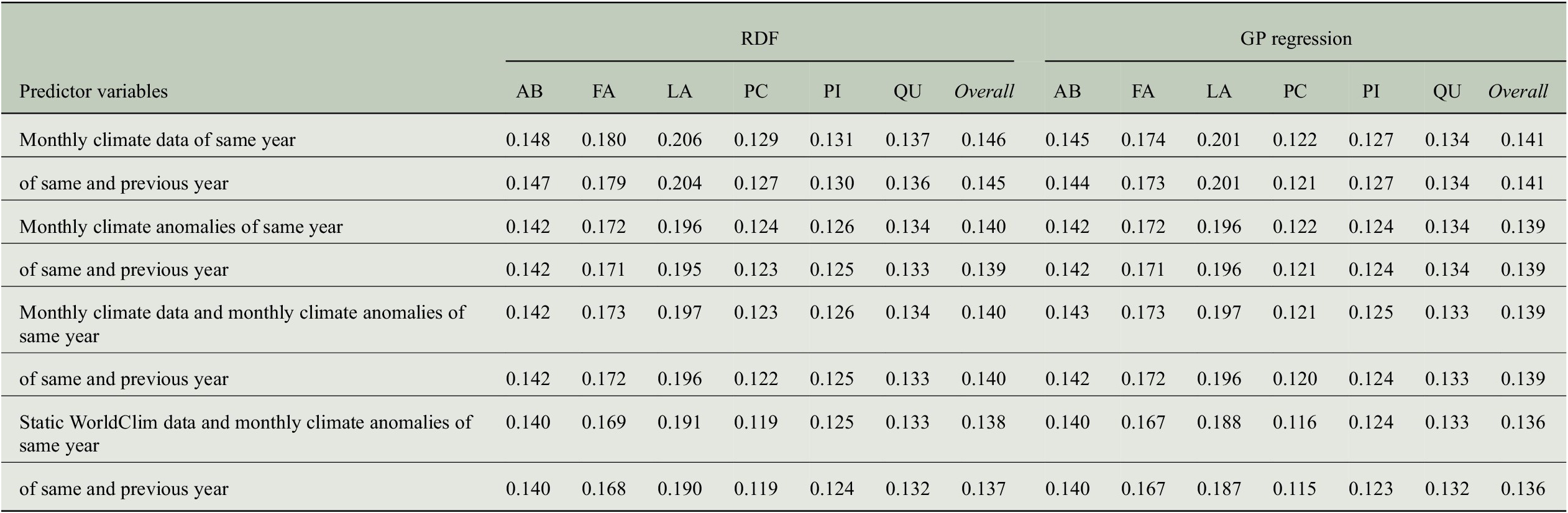
Abbreviations: GP, Gaussian process; RDF, random decision forest; RMSE, root-mean-square error.
Pearson correlation coefficients obtained from our leave-one-site-out experiments for predicting annual tree-ring indices.

Abbreviations: GP, Gaussian process; RDF, random decision forest.
Bias errors ( $ \times {10}^{-6} $
) of the MSE decomposition obtained from our leave-one-site-out experiments for predicting annual tree-ring indices.
$ \times {10}^{-6} $
) of the MSE decomposition obtained from our leave-one-site-out experiments for predicting annual tree-ring indices.

Note. Due to the indicated scaling factor, all bias errors are smaller than $ {10}^{-3} $
.
$ {10}^{-3} $
.
Abbreviations: GP, Gaussian process; MSE, mean-square error; RDF, random decision forest.
Variance errors of the MSE decomposition obtained from our leave-one-site-out experiments for predicting annual tree-ring indices.

Abbreviations: GP, Gaussian process; MSE, mean-square error; RDF, random decision forest.
Phase errors of the MSE decomposition obtained from our leave-one-site-out experiments for predicting annual tree-ring indices.

Abbreviations: GP, Gaussian process; MSE, mean-square error; RDF, random decision forest.
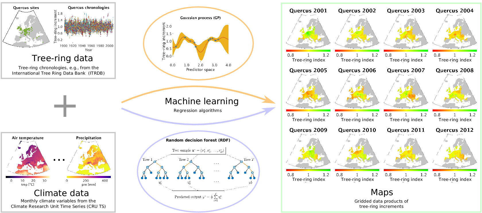
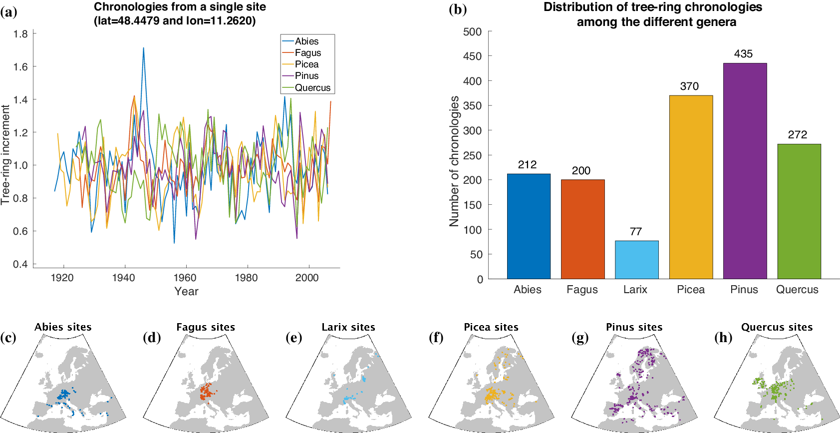


 Open access