


1. Introduction
Pioneers in turbulence research identified a universal pattern in the statistical moments of canonical flows. Within these universal regions, von Karman & Howarth (Reference von Karman and Howarth1938) were probably first to identify similarity solutions, also known as turbulent scaling laws. However, these laws were restricted to second-order moments. Self-preservation analysis, with a primary emphasis on turbulent shear flows and especially turbulent jet flows, has led to the derivation of classical scaling laws, exemplified by the seminal work of Townsend (Reference Townsend1956, Reference Townsend1976). Both laminar and turbulent jets show a strong tendency towards self-similarity. In the context of laminar round jet flow, an exact solution based on a similarity ansatz was provided by Schlichting (Reference Schlichting1933). Observations from various experiments suggest that turbulent round jet flows tend to reach a self-similar state in the far field (Wygnanski & Fiedler Reference Wygnanski and Fiedler1969; Panchapakesan & Lumley Reference Panchapakesan and Lumley1993a ; Hussein, Capp & George Reference Hussein, Capp and George1994).
Direct numerical simulations (DNSs) have emerged as powerful tools to investigate turbulent flows with unprecedented precision. To validate scaling laws, especially of higher-order moments, high-fidelity statistics are imperative, which can be achieved by DNSs. However, there have been limited DNS studies for turbulent round jet flows, especially those with a long box and incorporating an additional passive scalar. A passive scalar refers to a scalar quantity, such as temperature or the concentration of a chemical or contaminant, that does not influence the fluid flow. This concept applies specifically to cases where temperature variations are small and concentrations are dilute so that fluid properties are not affected. The Reynolds number $Re$
in these studies has often been kept low, and the averaging process has been limited to small time frames due to computational constraints. Notably, Boersma, Brethouwer & Nieuwstadt (Reference Boersma, Brethouwer and Nieuwstadt1998) initiated DNS for turbulent round jet flows, providing early insights into the influence of inflow conditions on self-similarity scaling in the far field at
$Re$
in these studies has often been kept low, and the averaging process has been limited to small time frames due to computational constraints. Notably, Boersma, Brethouwer & Nieuwstadt (Reference Boersma, Brethouwer and Nieuwstadt1998) initiated DNS for turbulent round jet flows, providing early insights into the influence of inflow conditions on self-similarity scaling in the far field at $Re=2400$
based on the orifice diameter. They imply that the collapse of the velocity and Reynolds stress profiles depends on the inflow conditions. However, they were unable to resolve the far field due to computational resources. As an extension of this work, Lubbers, Brethouwer & Boersma (Reference Lubbers, Brethouwer and Boersma2001) examined the self-similarity of a passive scalar concentration at
$Re=2400$
based on the orifice diameter. They imply that the collapse of the velocity and Reynolds stress profiles depends on the inflow conditions. However, they were unable to resolve the far field due to computational resources. As an extension of this work, Lubbers, Brethouwer & Boersma (Reference Lubbers, Brethouwer and Boersma2001) examined the self-similarity of a passive scalar concentration at $Re=2000$
as well and a Schmidt number
$Re=2000$
as well and a Schmidt number $Sc=1$
in a box with the length of
$Sc=1$
in a box with the length of $z/D=40$
where D is the jet orifice diameter. The statistics have been extracted over
$z/D=40$
where D is the jet orifice diameter. The statistics have been extracted over $80 D/U_b$
time units, where
$80 D/U_b$
time units, where $U_b$
refers to the bulk velocity at the inlet. The results show that the mean concentration in the far field is self-similar. However, the root mean square of the concentration fluctuations are not self-similar. In Babu & Mahesh (Reference Babu and Mahesh2005) a DNS of a turbulent jet at
$U_b$
refers to the bulk velocity at the inlet. The results show that the mean concentration in the far field is self-similar. However, the root mean square of the concentration fluctuations are not self-similar. In Babu & Mahesh (Reference Babu and Mahesh2005) a DNS of a turbulent jet at $Re=2400$
and
$Re=2400$
and $Sc=1$
is performed. The data are averaged over
$Sc=1$
is performed. The data are averaged over $1400 D/U_b$
time units. The instantaneous radial profiles of the velocity and passive scalar exhibit similarities and alternate between `top-hat’ and `triangle’ profiles, both spatially and temporally. These profiles are influenced by entrainment from the free stream into the jet, resulting in a mean Gaussian profile as a function of
$1400 D/U_b$
time units. The instantaneous radial profiles of the velocity and passive scalar exhibit similarities and alternate between `top-hat’ and `triangle’ profiles, both spatially and temporally. These profiles are influenced by entrainment from the free stream into the jet, resulting in a mean Gaussian profile as a function of $r$
. Diffusion-dominated regions are observed, occurring closer to the jet centre and as `brush-like’ regions near the jet edge. The width of these brush-like regions decreases with increasing
$r$
. Diffusion-dominated regions are observed, occurring closer to the jet centre and as `brush-like’ regions near the jet edge. The width of these brush-like regions decreases with increasing $Re$
, suggesting a transition in mixing behaviour. More recent simulations by Gilliland et al. (Reference Gilliland, Ranga-Dinesh, Fairweather, Falle, Jenkins and Savill2012) focused on a DNS at
$Re$
, suggesting a transition in mixing behaviour. More recent simulations by Gilliland et al. (Reference Gilliland, Ranga-Dinesh, Fairweather, Falle, Jenkins and Savill2012) focused on a DNS at $Re=2400$
and a large eddy simulation (LES) at
$Re=2400$
and a large eddy simulation (LES) at $Re=68\times 10^{3}$
in a box length of
$Re=68\times 10^{3}$
in a box length of $z/D=50$
to investigate scalar intermittency in a turbulent round jet. This simulation is quite recent and the averaging for both simulations was performed over approximately
$z/D=50$
to investigate scalar intermittency in a turbulent round jet. This simulation is quite recent and the averaging for both simulations was performed over approximately $900 D/U_b$
time units. The results emphasise the importance of external intermittency in scalar mixing. The study highlights the need for improved subgrid-scale models in LES to improve the accuracy of predicting external intermittency over a wide range of
$900 D/U_b$
time units. The results emphasise the importance of external intermittency in scalar mixing. The study highlights the need for improved subgrid-scale models in LES to improve the accuracy of predicting external intermittency over a wide range of $Re$
. Recently, we (Nguyen & Oberlack Reference Nguyen and Oberlack2024a
) were able to contribute to this field with a DNS of a spatially evolving round jet flow at
$Re$
. Recently, we (Nguyen & Oberlack Reference Nguyen and Oberlack2024a
) were able to contribute to this field with a DNS of a spatially evolving round jet flow at $Re=3500$
with a box length of
$Re=3500$
with a box length of $z/D=75$
. The statistics were averaged over
$z/D=75$
. The statistics were averaged over $75\,000 D/U_b$
time units, achieving an unsurpassed quality of DNS statistics for turbulent round jets. Notably, this DNS consists of a periodic turbulent pipe flow DNS as an inlet that ran simultaneously with the round jet DNS. Velocity moments up to the third order, and in a related publication (Nguyen & Oberlack Reference Nguyen and Oberlack2024b
) up to order ten, have been extracted, showing self-similarity, and probability density functions (PDFs) of the axial velocity over various radial distances from the centreline have also been collected.
$75\,000 D/U_b$
time units, achieving an unsurpassed quality of DNS statistics for turbulent round jets. Notably, this DNS consists of a periodic turbulent pipe flow DNS as an inlet that ran simultaneously with the round jet DNS. Velocity moments up to the third order, and in a related publication (Nguyen & Oberlack Reference Nguyen and Oberlack2024b
) up to order ten, have been extracted, showing self-similarity, and probability density functions (PDFs) of the axial velocity over various radial distances from the centreline have also been collected.
However, given that DNS was not feasible until the 1980s, many researchers opted for experimental approaches instead. In a notable study, Birch et al. (Reference Birch, Brown, Dodson and Thomas1978) conducted experiments measuring the turbulent concentration parameters of a free round methane jet up to the fourth moment. Their results revealed a departure from Gaussianity in the mean passive scalar concentration along the centreline, as indicated by the negative skewness of the PDF. Dowling & Dimotakis (Reference Dowling and Dimotakis1990) present an experimental investigation of the turbulent concentration field formed when a free turbulent jet at $Re=5000$
,
$Re=5000$
, $16\, \times \, 10^{3}$
,
$16\, \times \, 10^{3}$
, $40\, \times \, 10^{3}$
mixes with gas entrained from a quiescent reservoir at a Prandtl number
$40\, \times \, 10^{3}$
mixes with gas entrained from a quiescent reservoir at a Prandtl number $Pr=1{-}1.2$
. Laser-Rayleigh scattering measurements taken in the range
$Pr=1{-}1.2$
. Laser-Rayleigh scattering measurements taken in the range $z/D=20{-}90$
show a nearly independent behaviour with respect to the Reynolds number near the centreline of the jet for the scaled PDF of the jet fluid concentration. Antonia & Mi (Reference Antonia and Mi1993) have measured the average temperature dissipation using parallel cold wires at
$z/D=20{-}90$
show a nearly independent behaviour with respect to the Reynolds number near the centreline of the jet for the scaled PDF of the jet fluid concentration. Antonia & Mi (Reference Antonia and Mi1993) have measured the average temperature dissipation using parallel cold wires at $Re=19 \times 10^{3}$
and a Péclet number of
$Re=19 \times 10^{3}$
and a Péclet number of $Pe=83$
at a distance of
$Pe=83$
at a distance of $z/D=30$
from the orifice. The resulting components of the average temperature dissipation, particularly the radial and azimuthal values were found to be nearly equal, and only slightly larger than the axial component. The deviation from isotropy of the temperature dissipation was small, especially when compared with results in other free shear flows. In the work of Panchapakesan & Lumley (Reference Panchapakesan and Lumley1993b
), flying hot-wire measurements of a helium jet were made up to third-order moments, including mixed moments measured in the range
$z/D=30$
from the orifice. The resulting components of the average temperature dissipation, particularly the radial and azimuthal values were found to be nearly equal, and only slightly larger than the axial component. The deviation from isotropy of the temperature dissipation was small, especially when compared with results in other free shear flows. In the work of Panchapakesan & Lumley (Reference Panchapakesan and Lumley1993b
), flying hot-wire measurements of a helium jet were made up to third-order moments, including mixed moments measured in the range $z/D=50{-}120$
. The measurements, consistent with earlier studies of helium jets, provided insights into the mean velocity field, the concentration decay constant and the radial profiles of mean velocity and mean concentration. More recently, Darisse, Lemay & Benaïssa (Reference Darisse, Lemay and Benaïssa2015) studied a slightly heated turbulent round air jet at
$z/D=50{-}120$
. The measurements, consistent with earlier studies of helium jets, provided insights into the mean velocity field, the concentration decay constant and the radial profiles of mean velocity and mean concentration. More recently, Darisse, Lemay & Benaïssa (Reference Darisse, Lemay and Benaïssa2015) studied a slightly heated turbulent round air jet at $Re=14\times 10^{3}$
using temperature as a passive scalar. Laser Doppler velocimetry and laser Doppler velocimetry cold-wire thermometry measurements were performed for the variance, third-order moments and mixed moments at
$Re=14\times 10^{3}$
using temperature as a passive scalar. Laser Doppler velocimetry and laser Doppler velocimetry cold-wire thermometry measurements were performed for the variance, third-order moments and mixed moments at $z/D=30$
. This allows the investigation of all passive scalar transport budget terms except the dissipation term, which is derived by closing the balance. While previous studies, such as Birch et al. (Reference Birch, Brown, Dodson and Thomas1978), have ventured into the investigation of moments up to the fourth order in turbulent round jets, the investigation of moments beyond the third order has been relatively uncharted territory.
$z/D=30$
. This allows the investigation of all passive scalar transport budget terms except the dissipation term, which is derived by closing the balance. While previous studies, such as Birch et al. (Reference Birch, Brown, Dodson and Thomas1978), have ventured into the investigation of moments up to the fourth order in turbulent round jets, the investigation of moments beyond the third order has been relatively uncharted territory.
Turbulent scaling laws for higher-order moments can be systematically derived by applying symmetries in the underlying equations, a method known as Lie-symmetry analysis. In the pioneering work of Oberlack (Reference Oberlack2001), he used Lie-symmetry analysis in turbulence to generate invariant solutions, which are synonymous to turbulent scaling laws. Initially limited to the mean velocity, this approach was later expanded upon by Oberlack & Rosteck (Reference Oberlack and Rosteck2010). Their work recognised that the multi-point moment equations (MPMEs) harbour Lie symmetries not present in either the Euler or the Navier–Stokes equations, leading to the term `statistical symmetries’. This extension broadens the scope of Lie-symmetry analysis and allows for a more comprehensive understanding of higher-order moments in turbulent flows. In the realm of turbulence statistics, the commonly employed Reynolds decomposition
 \begin{equation} U_i=\overline {U}_i+u_i \end{equation}
prevails, where $\overline {(\cdot )}$
signifies time averaging,
$\overline {(\cdot )}$
signifies time averaging, $\overline {U}_i$
represents the mean velocity and
$\overline {U}_i$
represents the mean velocity and $u_i$
embodies turbulent fluctuations. This decomposition is equally applicable to the passive scalar concentration
$u_i$
embodies turbulent fluctuations. This decomposition is equally applicable to the passive scalar concentration
 \begin{equation} {\Theta} =\overline {\Theta }+\theta . \end{equation}
Within the Reynolds-averaged Navier–Stokes model, the instantaneous moment $H_{ij}=\overline {U_i U_j}$
undergoes a decomposition
$H_{ij}=\overline {U_i U_j}$
undergoes a decomposition
 \begin{equation} H_{ij}=\overline {U}_i \overline {U}_j +\overline {u_i u_j}, \end{equation}
leading to the emergence of the Reynolds stress tensor $R_{ij}=\overline {u_i u_j}$
. The introduction of
$R_{ij}=\overline {u_i u_j}$
. The introduction of $H_{ij}$
and
$H_{ij}$
and $R_{ij}$
distinguishes two distinct approaches: the omission of the Reynolds decomposition is called the
$R_{ij}$
distinguishes two distinct approaches: the omission of the Reynolds decomposition is called the $H$
-approach, while the conventional method is denoted as the
$H$
-approach, while the conventional method is denoted as the $R$
-approach. Analogously, the decomposition of the passive scalar concentration extends to
$R$
-approach. Analogously, the decomposition of the passive scalar concentration extends to
 \begin{equation} H_{\Theta \Theta }=\overline {\Theta }^{2}+R_{\Theta \Theta }, \end{equation}
or mixed moments denoted by
 \begin{equation} H_{i\Theta }=\overline {U_i}\,\overline {\Theta }+R_{i\Theta }, \end{equation}
where $R_{\Theta \Theta }=\overline {\theta ^{2}}$
and
$R_{\Theta \Theta }=\overline {\theta ^{2}}$
and $R_{i\Theta } =\overline {u_i \theta }$
. Focusing on the MPMEs based on instantaneous velocities yields an infinite set of linear equations, where coupling occurs only between `neighbouring’ equations. The identification of symmetries within the MPMEs allows for the derivation of invariant solutions, providing a rigorous basis for turbulent scaling laws. Notably, in the works of Sadeghi et al. (Reference Sadeghi, Oberlack and Gauding2018, Reference Sadeghi, Oberlack and Gauding2021), this method has demonstrated success not only for velocity moments but also for passive scalar moments up to the second order in temporally evolving turbulent plane jets. Recent contributions by Oberlack et al. (Reference Oberlack, Hoyas, Kraheberger, Alcántara-Ávila and Laux2022) extended the application of this methodology, deriving turbulent scaling laws for moments of arbitrary order in the log and the core region of a turbulent channel flow. The derived laws were successfully validated through a new DNS of a Poiseuille channel flow at a friction Reynolds number of
$R_{i\Theta } =\overline {u_i \theta }$
. Focusing on the MPMEs based on instantaneous velocities yields an infinite set of linear equations, where coupling occurs only between `neighbouring’ equations. The identification of symmetries within the MPMEs allows for the derivation of invariant solutions, providing a rigorous basis for turbulent scaling laws. Notably, in the works of Sadeghi et al. (Reference Sadeghi, Oberlack and Gauding2018, Reference Sadeghi, Oberlack and Gauding2021), this method has demonstrated success not only for velocity moments but also for passive scalar moments up to the second order in temporally evolving turbulent plane jets. Recent contributions by Oberlack et al. (Reference Oberlack, Hoyas, Kraheberger, Alcántara-Ávila and Laux2022) extended the application of this methodology, deriving turbulent scaling laws for moments of arbitrary order in the log and the core region of a turbulent channel flow. The derived laws were successfully validated through a new DNS of a Poiseuille channel flow at a friction Reynolds number of $10^4$
. Alcántara-Ávila et al. (Reference Alcántara-Ávila, García-Raffi, Miguel, Hoyas and Oberlack2024) expanded on this with symmetry-based turbulent scaling laws for streamwise velocity and temperature moments of arbitrary order for the core region of a turbulent channel which have been validated by DNS of various Reynolds numbers. In it, the authors also derived the MPMEs for a scalar and for mixed scalar–velocity moments for the first time, which are also used here.
$10^4$
. Alcántara-Ávila et al. (Reference Alcántara-Ávila, García-Raffi, Miguel, Hoyas and Oberlack2024) expanded on this with symmetry-based turbulent scaling laws for streamwise velocity and temperature moments of arbitrary order for the core region of a turbulent channel which have been validated by DNS of various Reynolds numbers. In it, the authors also derived the MPMEs for a scalar and for mixed scalar–velocity moments for the first time, which are also used here.
In our recent work (Nguyen & Oberlack Reference Nguyen and Oberlack2024b ), we applied Lie-symmetry analysis to a spatially evolving turbulent round jet flow, where we were able to derive turbulent velocity scaling laws up to an arbitrary order and validate them against DNS data of velocity moments of up to tenth order. Furthermore, it was found that the effects of intermittency are hidden in the symmetries of the governing equations, highlighting the importance of Lie-symmetry analysis in improving our understanding of turbulence.
In this work, DNS data on a passive scalar shall be presented and made available to the community. In addition, this versatile method of Lie-symmetry analysis is intended to be applied to the multi-point scalar equation and the multi-point velocity–scalar equation for a turbulent round jet flow. Although DNSs are computationally expensive, they are required to compute high-quality moments of higher order. A LES, although less expensive, and therefore allowing for higher Reynolds numbers, does not fulfil this requirement.
2. Governing equations
The governing equations for the present study are the Navier–Stokes equations (NSEs) describing incompressible flow. They are composed of the continuity equation
 \begin{equation} \nabla \cdot \boldsymbol{U}=0 ,\end{equation}
and the momentum balance equations
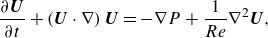 \begin{equation} \frac {\partial \boldsymbol{U}}{\partial t}+\left ( \boldsymbol{U} \cdot \nabla \right ) \boldsymbol{U}=- \nabla P+\frac {1}{Re} \nabla ^{2} \boldsymbol{U}, \end{equation}
where $\boldsymbol{U}$
,
$\boldsymbol{U}$
, $P$
and
$P$
and $t$
represent the velocity vector, pressure and time, respectively, and the Reynolds number is defined as
$t$
represent the velocity vector, pressure and time, respectively, and the Reynolds number is defined as
 \begin{equation} Re=\frac {U_b D}{\nu }, \end{equation}
where $U_b$
,
$U_b$
, $D$
and
$D$
and $\nu$
are the bulk velocity at the orifice, the diameter at the orifice and the kinematic viscosity, respectively. In addition, a convection–diffusion equation governs the behaviour of a passive scalar
$\nu$
are the bulk velocity at the orifice, the diameter at the orifice and the kinematic viscosity, respectively. In addition, a convection–diffusion equation governs the behaviour of a passive scalar
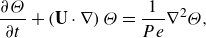 \begin{equation} \frac {\partial \Theta }{\partial t} +\left ( \textbf{U} \cdot \nabla \right ) \Theta =\frac {1}{Pe}\nabla ^{2} \Theta , \end{equation}
where $\Theta$
denotes the passive scalar, and
$\Theta$
denotes the passive scalar, and $Pe$
is the Péclet number, defined as the product of the Reynolds number and the Prandtl number, i.e.
$Pe$
is the Péclet number, defined as the product of the Reynolds number and the Prandtl number, i.e. $Pe=Re \, Pr$
. Here,
$Pe=Re \, Pr$
. Here, $\Theta$
is bound by the boundary and initial conditions of a given physical problem.
$\Theta$
is bound by the boundary and initial conditions of a given physical problem.
3. Direct numerical simulation details
The numerical solution of the NSEs is performed with Nek5000, a solver developed by Fischer, Lottes & Kerkemeier (Reference Fischer, Lottes and Kerkemeier2008) based on a high-order spectral element method outlined in Patera (Reference Patera1984). For optimal efficiency, a polynomial order of $N=7$
is selected and the backward differentiation formula of second order (BDF2) scheme is employed for time stepping. The DNS of the turbulent round jet flow is conducted at
$N=7$
is selected and the backward differentiation formula of second order (BDF2) scheme is employed for time stepping. The DNS of the turbulent round jet flow is conducted at $Re=3500$
, with a box length of
$Re=3500$
, with a box length of $z/D=75$
. A fully turbulent velocity profile of a pipe flow is imposed at the inlet, and on-the-fly statistical averaging is performed for each time step over
$z/D=75$
. A fully turbulent velocity profile of a pipe flow is imposed at the inlet, and on-the-fly statistical averaging is performed for each time step over $75\,000 D/U_b$
units. Despite the significantly larger box, this corresponds to nearly 200 passes of a particle through the entire computational domain of the jet. A detailed description of the DNS methodology can be found in Nguyen & Oberlack (Reference Nguyen and Oberlack2024a
). In addition, a passive scalar is solved using (2.4) for air at
$75\,000 D/U_b$
units. Despite the significantly larger box, this corresponds to nearly 200 passes of a particle through the entire computational domain of the jet. A detailed description of the DNS methodology can be found in Nguyen & Oberlack (Reference Nguyen and Oberlack2024a
). In addition, a passive scalar is solved using (2.4) for air at $Pr=0.71$
, which can be interpreted as the heat conduction of air. Buoyancy effects have been explicitly excluded, i.e. this scalar can be considered passive since the fluid is incompressible (
$Pr=0.71$
, which can be interpreted as the heat conduction of air. Buoyancy effects have been explicitly excluded, i.e. this scalar can be considered passive since the fluid is incompressible ( $\rho = \textrm{const.}$
, where
$\rho = \textrm{const.}$
, where $\rho$
denotes the density) and hence unaffected by gravity. The passive scalar is introduced at the inlet as a top-hat profile with
$\rho$
denotes the density) and hence unaffected by gravity. The passive scalar is introduced at the inlet as a top-hat profile with $\Theta =1$
. At
$\Theta =1$
. At $z/D=0$
outside the jet inlet, the passive scalar is set to zero. To avoid unphysical behaviour, the thermal open boundary condition, as introduced in Liu, Xie & Dong (Reference Liu, Xie and Dong2020), is implemented for the passive scalar at the lateral boundaries and at the jet outlet at
$z/D=0$
outside the jet inlet, the passive scalar is set to zero. To avoid unphysical behaviour, the thermal open boundary condition, as introduced in Liu, Xie & Dong (Reference Liu, Xie and Dong2020), is implemented for the passive scalar at the lateral boundaries and at the jet outlet at $z/D=75$
.
$z/D=75$
.
4. Passive scalar statistics
In this section, we delve into a detailed investigation of the statistical properties associated with the passive scalar concentration in turbulent round jet flows. Leveraging insights from the DNS, we explore various facets of the passive scalar field, ranging from mean concentration profiles to higher-order statistical moments and PDFs. Through rigorous comparisons with previous experimental results, we aim to outline both agreements and differences, providing a comprehensive view of the dynamics governing turbulent round jet flows.
4.1. Mean passive scalar statistics
The mean passive scalar concentration $\overline {\Theta }_c$
is scaled by the mean centreline concentration, which is linearly related to the distance from the orifice
$\overline {\Theta }_c$
is scaled by the mean centreline concentration, which is linearly related to the distance from the orifice
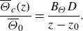 \begin{equation} \frac {\overline {\Theta }_c(z)}{\overline {\Theta }_0}=\frac {B_\Theta D}{z-z_0}. \end{equation}
From the present DNS, we deduce a decay constant of $B_\Theta =4.9$
with a virtual origin at
$B_\Theta =4.9$
with a virtual origin at $z_0/D=-0.132$
, which means the virtual origin is close to the virtual origin of the velocity
$z_0/D=-0.132$
, which means the virtual origin is close to the virtual origin of the velocity $z_0/D=0$
(Nguyen & Oberlack Reference Nguyen and Oberlack2024a
) taken from the classical velocity scaling (Boersma et al. Reference Boersma, Brethouwer and Nieuwstadt1998)
$z_0/D=0$
(Nguyen & Oberlack Reference Nguyen and Oberlack2024a
) taken from the classical velocity scaling (Boersma et al. Reference Boersma, Brethouwer and Nieuwstadt1998)
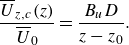 \begin{equation} \frac {\overline {U}_{z,c}(z)}{\overline {U}_0}=\frac {B_u D}{z-z_0}. \end{equation}
Mean inverse passive scalar concentration at the centreline over the distance of the orifice: Birch et al. (Reference Birch, Brown, Dodson and Thomas1978) (![]() ), Babu & Mahesh (Reference Babu and Mahesh2005) (
), Babu & Mahesh (Reference Babu and Mahesh2005) (![]() ), Lubbers et al. (Reference Lubbers, Brethouwer and Boersma2001) (
), Lubbers et al. (Reference Lubbers, Brethouwer and Boersma2001) (![]() ), present DNS (
), present DNS (![]() ).
).
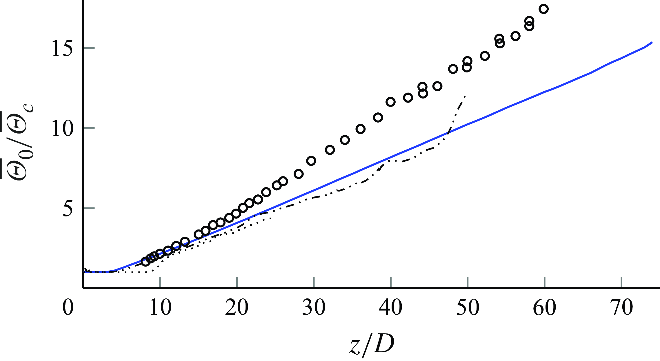
This is compared with Lubbers et al. (Reference Lubbers, Brethouwer and Boersma2001), where they found $z_0/D=0.5$
for the concentration and
$z_0/D=0.5$
for the concentration and $z_0/D=5.5$
for the axial velocity. Figure 1 showcases a consistent and smoother linear trend of the inverse passive scalar concentration up to
$z_0/D=5.5$
for the axial velocity. Figure 1 showcases a consistent and smoother linear trend of the inverse passive scalar concentration up to $z/D=75$
compared with other experiments and DNS. A collection of the data from the experiments shown in figure 1 can be found in table 1.
$z/D=75$
compared with other experiments and DNS. A collection of the data from the experiments shown in figure 1 can be found in table 1.
Various jet parameters of DNS and experiments.
For the velocity the decay constant is $B_u=5.15$
(Nguyen & Oberlack Reference Nguyen and Oberlack2024a
), implying that
$B_u=5.15$
(Nguyen & Oberlack Reference Nguyen and Oberlack2024a
), implying that $\overline {\Theta }_c$
decays faster than the velocity. Lubbers et al. (Reference Lubbers, Brethouwer and Boersma2001) have observed the same, but their virtual origins for the velocity and the passive scalar concentration were further apart. The value of
$\overline {\Theta }_c$
decays faster than the velocity. Lubbers et al. (Reference Lubbers, Brethouwer and Boersma2001) have observed the same, but their virtual origins for the velocity and the passive scalar concentration were further apart. The value of $\overline {\Theta }_c$
reaches self-similarity at
$\overline {\Theta }_c$
reaches self-similarity at $z/D=15$
, as depicted in figure 2. This onset occurs earlier than the assumed
$z/D=15$
, as depicted in figure 2. This onset occurs earlier than the assumed $z/D=20$
in Lubbers et al. (Reference Lubbers, Brethouwer and Boersma2001). Upon comparing the profile of
$z/D=20$
in Lubbers et al. (Reference Lubbers, Brethouwer and Boersma2001). Upon comparing the profile of $\overline {U}_{z,c}$
with that of
$\overline {U}_{z,c}$
with that of $\overline {\Theta }_c$
, the latter shows a slightly larger spreading rate. The Prandtl number describes the relative thicknesses of the velocity and thermal boundary layers. With
$\overline {\Theta }_c$
, the latter shows a slightly larger spreading rate. The Prandtl number describes the relative thicknesses of the velocity and thermal boundary layers. With $Pr=0.71$
, the thermal boundary layer is thicker than the velocity boundary layer, leading to a larger spreading rate. The half-width of the mean passive scalar concentration,
$Pr=0.71$
, the thermal boundary layer is thicker than the velocity boundary layer, leading to a larger spreading rate. The half-width of the mean passive scalar concentration, $\eta _{1/2,\Theta }=0.109$
, exceeds that of the velocity,
$\eta _{1/2,\Theta }=0.109$
, exceeds that of the velocity, $\eta _{1/2,u}=0.089$
, as reported in Nguyen & Oberlack (Reference Nguyen and Oberlack2024a
), where
$\eta _{1/2,u}=0.089$
, as reported in Nguyen & Oberlack (Reference Nguyen and Oberlack2024a
), where $\eta =r/(z-z_0)$
is the usual jet-type similarity coordinate, as derived below in (5.20). Remarkably,
$\eta =r/(z-z_0)$
is the usual jet-type similarity coordinate, as derived below in (5.20). Remarkably, $\eta _{1/2,\Theta }$
closely aligns with the observation in Lubbers et al. (Reference Lubbers, Brethouwer and Boersma2001), where
$\eta _{1/2,\Theta }$
closely aligns with the observation in Lubbers et al. (Reference Lubbers, Brethouwer and Boersma2001), where $\eta _{1/2,\Theta }=0.108$
in their DNS.
$\eta _{1/2,\Theta }=0.108$
in their DNS.
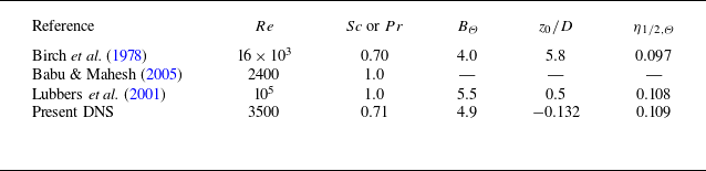
Mean passive scalar $\overline {\Theta }$
scaled with the centreline passive scalar concentration
$\overline {\Theta }$
scaled with the centreline passive scalar concentration $\overline {\Theta }_c$
and plotted as a function of the similarity coordinate
$\overline {\Theta }_c$
and plotted as a function of the similarity coordinate $\eta$
(see (5.20)) at different distances from the orifice:
$\eta$
(see (5.20)) at different distances from the orifice: $z/D=15$
(
$z/D=15$
(![]() ),
), $25$
(
$25$
(![]() ),
), $35$
(
$35$
(![]() ),
), $45$
(
$45$
(![]() ),
), $55$
(
$55$
(![]() ).
).
In summary, the characteristics of $\overline {\Theta }_c$
are consistent with those observed by Lubbers et al. (Reference Lubbers, Brethouwer and Boersma2001). The profiles exhibit self-similarity and a faster spread compared with the velocity profile. Moreover, the virtual origins of concentration and velocity appear to have shifted closer to each other compared with the DNS by Lubbers et al. (Reference Lubbers, Brethouwer and Boersma2001), which is attributed to the turbulent pipe inlet.
$\overline {\Theta }_c$
are consistent with those observed by Lubbers et al. (Reference Lubbers, Brethouwer and Boersma2001). The profiles exhibit self-similarity and a faster spread compared with the velocity profile. Moreover, the virtual origins of concentration and velocity appear to have shifted closer to each other compared with the DNS by Lubbers et al. (Reference Lubbers, Brethouwer and Boersma2001), which is attributed to the turbulent pipe inlet.
4.2. Second-order passive scalar and mixed statistics
The variance of the passive scalar fluctuation $R_{\Theta \Theta }$
is shown in figure 3 for different distances
$R_{\Theta \Theta }$
is shown in figure 3 for different distances $z$
from the orifice. The value at
$z$
from the orifice. The value at $\eta =0$
agrees with the results of Lubbers et al. (Reference Lubbers, Brethouwer and Boersma2001) and Darisse et al. (Reference Darisse, Lemay and Benaïssa2015), both of which report values around
$\eta =0$
agrees with the results of Lubbers et al. (Reference Lubbers, Brethouwer and Boersma2001) and Darisse et al. (Reference Darisse, Lemay and Benaïssa2015), both of which report values around $0.04$
and slightly above. However, the off-axis peak exceeds the value of
$0.04$
and slightly above. However, the off-axis peak exceeds the value of $0.05$
measured by Darisse et al. (Reference Darisse, Lemay and Benaïssa2015). The peak is at
$0.05$
measured by Darisse et al. (Reference Darisse, Lemay and Benaïssa2015). The peak is at $\eta =0.082$
, which is slightly towards the centre of the inflection point of the passive scalar profile in figure 2 at
$\eta =0.082$
, which is slightly towards the centre of the inflection point of the passive scalar profile in figure 2 at $\eta =0.089$
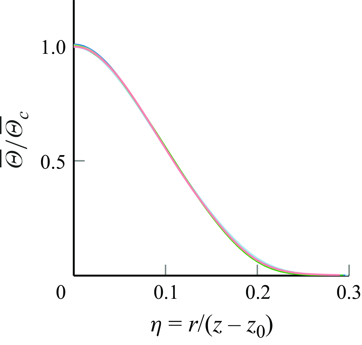
. The inflection point in the scalar profile corresponds to the region where the scalar is being transported most effectively from the jet core to the surrounding fluid. In turbulent round jet flows, turbulent eddies begin to form at the edge of the jet inlet. These eddies grow and interact with the scalar field as the jet develops. This process enhances the mixing of the scalar within the shear layer between jet and the surrounding ambient fluid, leading to fluctuations in the scalar field. The mixing begins slightly inside the region where the scalar gradient is steepest which may lead to the peak in fluctuations on the centre-facing side of the inflection point.
$\eta =0.089$
. The inflection point in the scalar profile corresponds to the region where the scalar is being transported most effectively from the jet core to the surrounding fluid. In turbulent round jet flows, turbulent eddies begin to form at the edge of the jet inlet. These eddies grow and interact with the scalar field as the jet develops. This process enhances the mixing of the scalar within the shear layer between jet and the surrounding ambient fluid, leading to fluctuations in the scalar field. The mixing begins slightly inside the region where the scalar gradient is steepest which may lead to the peak in fluctuations on the centre-facing side of the inflection point.
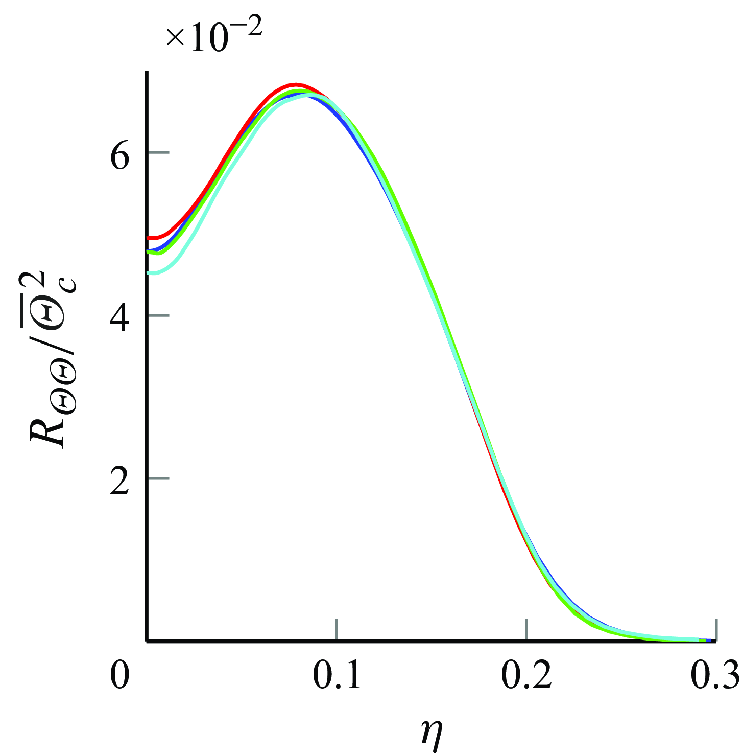
Variance of the passive scalar fluctuations $R_{\Theta \Theta }$
scaled with the centreline passive scalar concentration
$R_{\Theta \Theta }$
scaled with the centreline passive scalar concentration $\overline {\Theta }^{2}_c$
and plotted as a function of the similarity coordinate
$\overline {\Theta }^{2}_c$
and plotted as a function of the similarity coordinate $\eta$
at different distances from the orifice:
$\eta$
at different distances from the orifice: $z/D=25$
(
$z/D=25$
(![]() ),
), $35$
(
$35$
(![]() ),
), $45$
(
$45$
(![]() ),
), $55$
(
$55$
(![]() ).
).
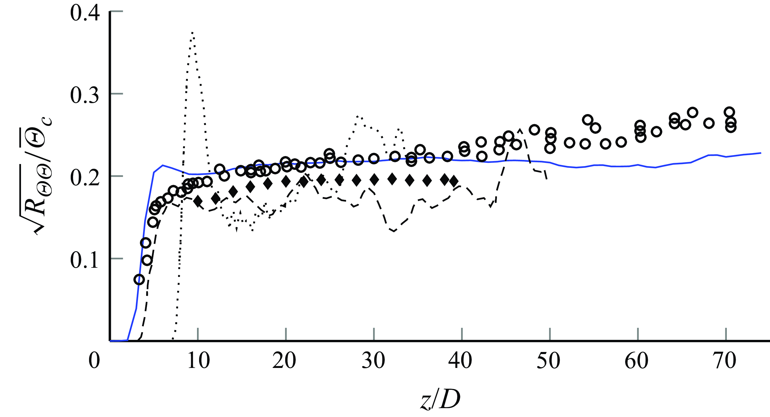
Lubbers et al. (Reference Lubbers, Brethouwer and Boersma2001) notes in figure 4 that the normalised root mean square (r.m.s.) of the passive scalar fluctuation $\sqrt {R_{\Theta \Theta }}$
shows an increasing trend rather than a horizontal line, the former indicating non-self-similarity. This trend can be attributed to the smaller axial length of their computational box, as the present DNS shows a slight increase up to
$\sqrt {R_{\Theta \Theta }}$
shows an increasing trend rather than a horizontal line, the former indicating non-self-similarity. This trend can be attributed to the smaller axial length of their computational box, as the present DNS shows a slight increase up to $z/D=35$
. After this point, however,
$z/D=35$
. After this point, however, $\sqrt {R_{\Theta \Theta }}$
stabilises around
$\sqrt {R_{\Theta \Theta }}$
stabilises around $0.22$
, supporting Dowling & Dimotakis’s (Reference Dowling and Dimotakis1990) conclusion that
$0.22$
, supporting Dowling & Dimotakis’s (Reference Dowling and Dimotakis1990) conclusion that $\sqrt {R_{\Theta \Theta }}$
lies between
$\sqrt {R_{\Theta \Theta }}$
lies between $0.23$
and
$0.23$
and $0.24$
, with the present DNS slightly below this range.
$0.24$
, with the present DNS slightly below this range.
Centreline r.m.s. of the passive scalar fluctuation $\sqrt {R_{\Theta \Theta }}$
scaled with the centreline mean passive scalar concentration over the distance
$\sqrt {R_{\Theta \Theta }}$
scaled with the centreline mean passive scalar concentration over the distance $z$
from the orifice: Darisse et al. (Reference Darisse, Lemay and Benaïssa2015) (
$z$
from the orifice: Darisse et al. (Reference Darisse, Lemay and Benaïssa2015) (![]() ), Birch et al. (Reference Birch, Brown, Dodson and Thomas1978) (
), Birch et al. (Reference Birch, Brown, Dodson and Thomas1978) (![]() ), Babu & Mahesh (Reference Babu and Mahesh2005) (
), Babu & Mahesh (Reference Babu and Mahesh2005) (![]() ), Lubbers et al. (Reference Lubbers, Brethouwer and Boersma2001) (
), Lubbers et al. (Reference Lubbers, Brethouwer and Boersma2001) (![]() ), present DNS (
), present DNS (![]() ).
).
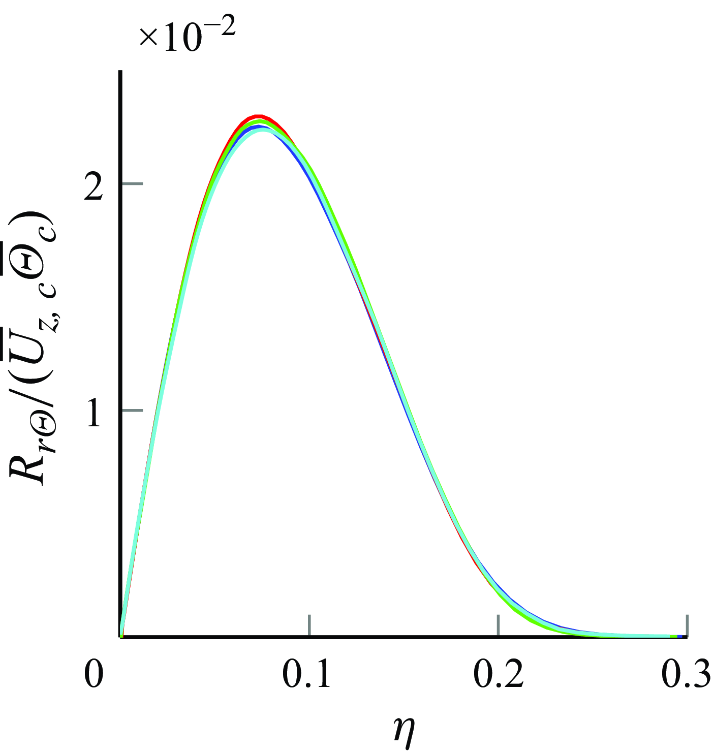
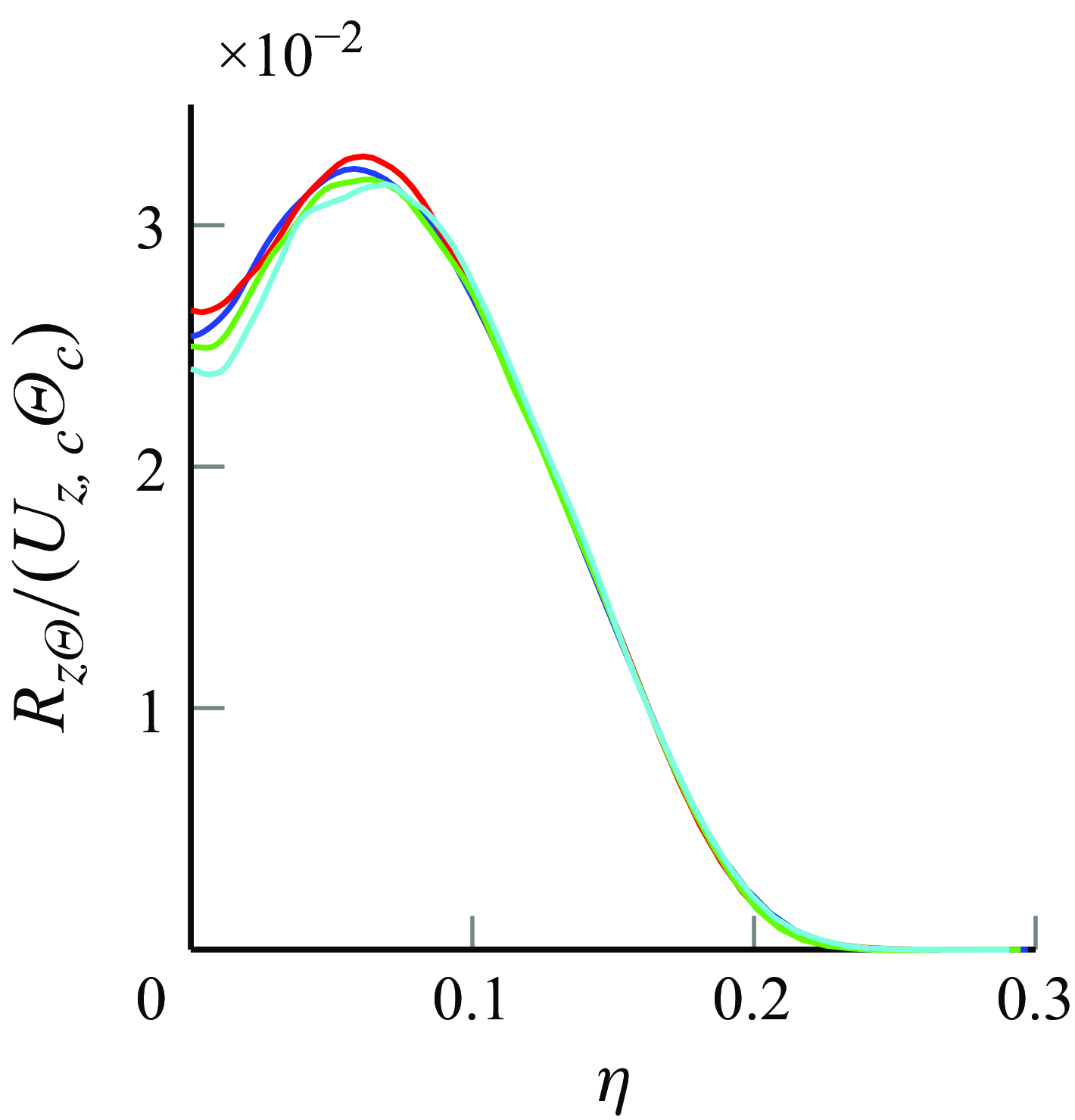
The turbulent diffusive fluxes shown in figures 5 and 6 exhibit a close resemblance to the radial profiles in Darisse et al. (Reference Darisse, Lemay and Benaïssa2015). The measured maximum values for $R_{r\Theta }/(\overline {U}_{z,c}\overline {\Theta }_c)$
and
$R_{r\Theta }/(\overline {U}_{z,c}\overline {\Theta }_c)$
and $R_{z\Theta }/(\overline {U}_{z,c}\overline {\Theta }_c)$
in Darisse et al. (Reference Darisse, Lemay and Benaïssa2015) are
$R_{z\Theta }/(\overline {U}_{z,c}\overline {\Theta }_c)$
in Darisse et al. (Reference Darisse, Lemay and Benaïssa2015) are $2.2$
and
$2.2$
and $3$
, respectively, consistent with the
$3$
, respectively, consistent with the $2.2$
and
$2.2$
and $3.2$
values observed in figures 5 and 6. In addition, the value at
$3.2$
values observed in figures 5 and 6. In addition, the value at $\eta =0$
for
$\eta =0$
for $R_{z\Theta }/(\overline {U}_{z,c}\overline {\Theta }_c)$
is approximately
$R_{z\Theta }/(\overline {U}_{z,c}\overline {\Theta }_c)$
is approximately $0.024$
in Darisse et al. (Reference Darisse, Lemay and Benaïssa2015), closely matching the range of
$0.024$
in Darisse et al. (Reference Darisse, Lemay and Benaïssa2015), closely matching the range of $0.025-0.026$
in the present DNS.
$0.025-0.026$
in the present DNS.
Turbulent heat flux $R_{r\Theta }$
normalised with
$R_{r\Theta }$
normalised with $\overline {U}_{z,c}\overline {\Theta }_c$
at different distances from the orifice:
$\overline {U}_{z,c}\overline {\Theta }_c$
at different distances from the orifice: $z/D=25$
(
$z/D=25$
(![]() ),
), $35$
(
$35$
(![]() ),
), $45$
(
$45$
(![]() ),
), $55$
(
$55$
(![]() ).
).
Turbulent heat flux $R_{z\Theta }$
normalised with
$R_{z\Theta }$
normalised with $\overline {U}_{z,c}\overline {\Theta }_c$
at different distances from the orifice:
$\overline {U}_{z,c}\overline {\Theta }_c$
at different distances from the orifice: $z/D=25$
(
$z/D=25$
(![]() ),
), $35$
(
$35$
(![]() ),
), $45$
(
$45$
(![]() ),
), $55$
(
$55$
(![]() ).
).
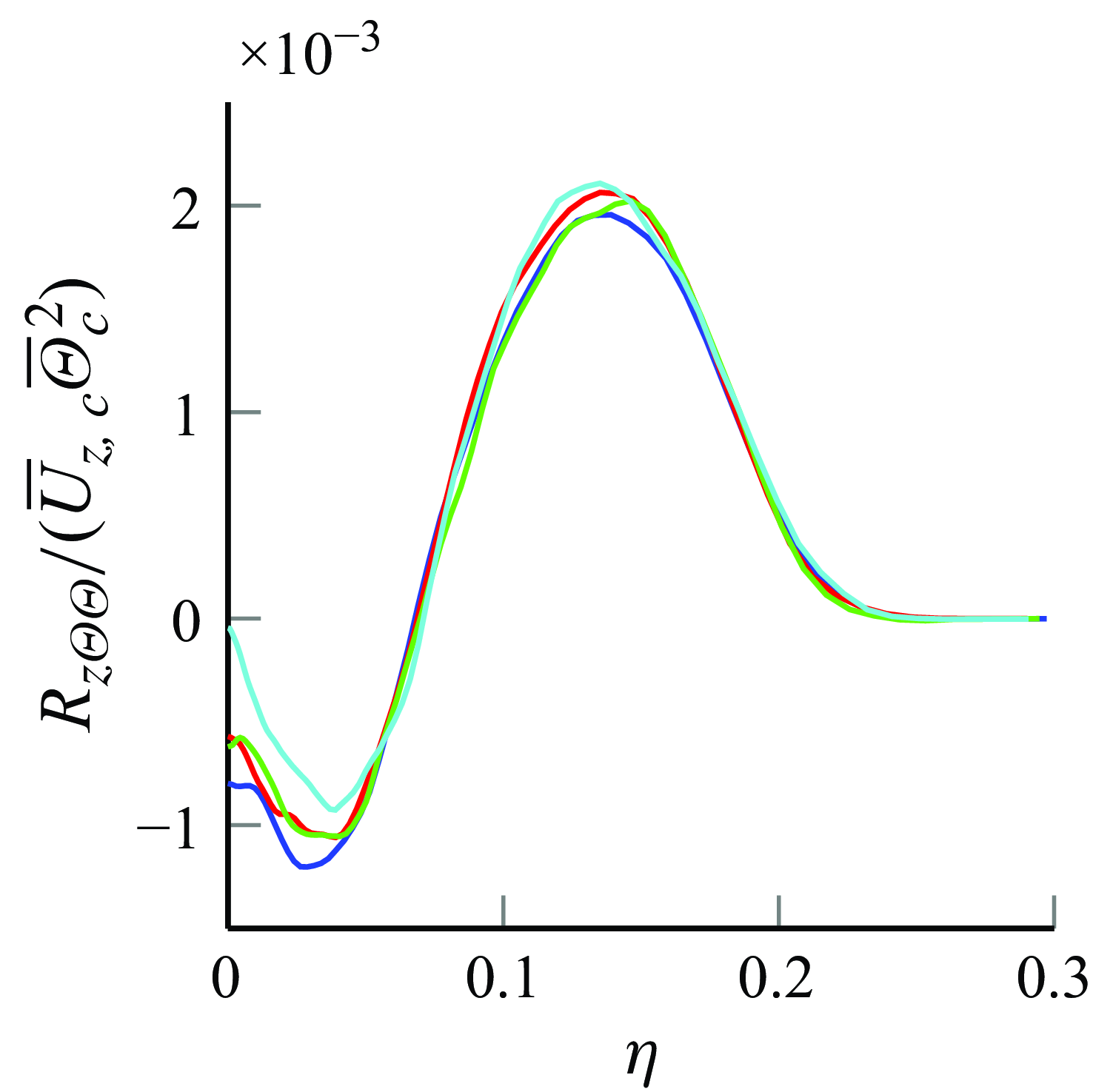
4.3. Third-order mixed statistics
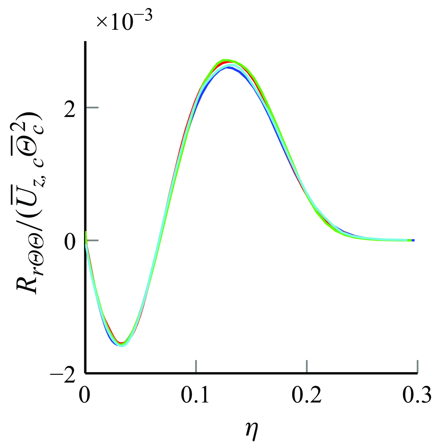
There are only quite few experimental data on the radial profiles of the third-order mixed statistics $R_{i\Theta \Theta }$
, due to their sensitivity to disturbances in experimental set-ups. In contrast, the present DNS provides a well-converged data set, allowing a detailed examination of these statistics. Comparable experiments are mainly the helium jet of Panchapakesan & Lumley (Reference Panchapakesan and Lumley1993b
) and the heated jet by Darisse et al. (Reference Darisse, Lemay and Benaïssa2015), which provide a basis for validation. Notably, Antonia, Prabhu & Stephenson (Reference Antonia, Prabhu and Stephenson1975) also contributed data for
$R_{i\Theta \Theta }$
, due to their sensitivity to disturbances in experimental set-ups. In contrast, the present DNS provides a well-converged data set, allowing a detailed examination of these statistics. Comparable experiments are mainly the helium jet of Panchapakesan & Lumley (Reference Panchapakesan and Lumley1993b
) and the heated jet by Darisse et al. (Reference Darisse, Lemay and Benaïssa2015), which provide a basis for validation. Notably, Antonia, Prabhu & Stephenson (Reference Antonia, Prabhu and Stephenson1975) also contributed data for $R_{i\Theta \Theta }$
, although using a jet with a strong co-flow. Nevertheless, the shape of the data is similar to the experiments of Darisse et al. (Reference Darisse, Lemay and Benaïssa2015), but with different magnitudes. The radial profiles of the normalised third-order mixed statistics of the present DNS are showcased in figures 7 and 8 for
$R_{i\Theta \Theta }$
, although using a jet with a strong co-flow. Nevertheless, the shape of the data is similar to the experiments of Darisse et al. (Reference Darisse, Lemay and Benaïssa2015), but with different magnitudes. The radial profiles of the normalised third-order mixed statistics of the present DNS are showcased in figures 7 and 8 for $R_{r\Theta \Theta }$
and
$R_{r\Theta \Theta }$
and $R_{z\Theta \Theta }$
, respectively. Qualitatively, the shapes of the aforementioned experiments are similar to those of the present DNS. While the maxima of the present DNS closely match Darisse et al. (Reference Darisse, Lemay and Benaïssa2015), the minima have slightly larger magnitudes, and Panchapakesan & Lumley (Reference Panchapakesan and Lumley1993b
) presents an even larger minimum for
$R_{z\Theta \Theta }$
, respectively. Qualitatively, the shapes of the aforementioned experiments are similar to those of the present DNS. While the maxima of the present DNS closely match Darisse et al. (Reference Darisse, Lemay and Benaïssa2015), the minima have slightly larger magnitudes, and Panchapakesan & Lumley (Reference Panchapakesan and Lumley1993b
) presents an even larger minimum for $R_{r\Theta \Theta }$
.
$R_{r\Theta \Theta }$
.
Turbulent heat flux $R_{r\Theta \Theta }$
normalised with
$R_{r\Theta \Theta }$
normalised with $\overline {U}_{z,c}\overline {\Theta }_c^{2}$
at different distances from the orifice:
$\overline {U}_{z,c}\overline {\Theta }_c^{2}$
at different distances from the orifice: $z/D=25$
(
$z/D=25$
(![]() ),
), $35$
(
$35$
(![]() ),
), $45$
(
$45$
(![]() ),
), $55$
(
$55$
(![]() ).
).
Turbulent heat flux $R_{z\Theta \Theta }$
normalised with
$R_{z\Theta \Theta }$
normalised with $\overline {U}_{z,c}\overline {\Theta }_c^{2}$
at different distances from the orifice:
$\overline {U}_{z,c}\overline {\Theta }_c^{2}$
at different distances from the orifice: $z/D=25$
(
$z/D=25$
(![]() ),
), $35$
(
$35$
(![]() ),
), $45$
(
$45$
(![]() ),
), $55$
(
$55$
(![]() ).
).
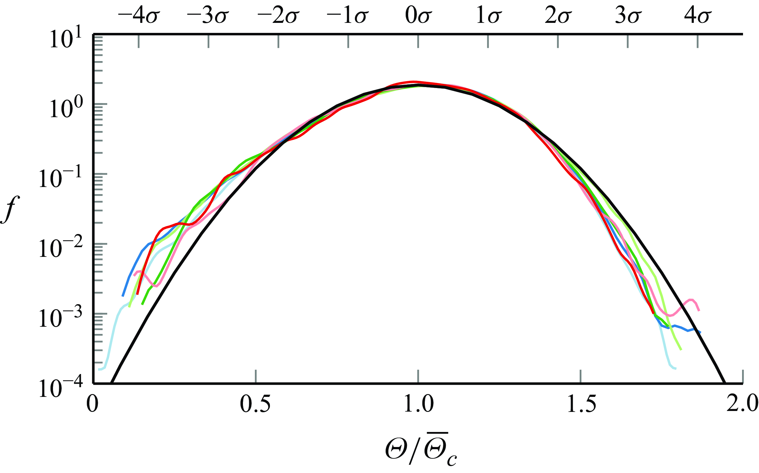
4.4. Probability density functions
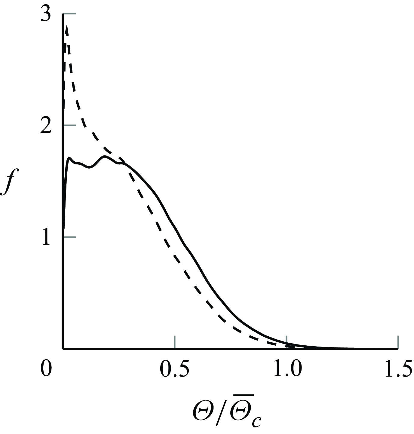
In figure 9, the PDFs of the passive scalar concentration on the centreline at different orifice distances exhibit excellent collapse, closely resembling a Gaussian distribution. The PDFs are slightly negatively skewed, which can also be read off in figure 11 at $\eta =0$
. The negative skewness on the centreline for a passive scalar concentration was also observed in the methane jet of Birch et al. (Reference Birch, Brown, Dodson and Thomas1978).
$\eta =0$
. The negative skewness on the centreline for a passive scalar concentration was also observed in the methane jet of Birch et al. (Reference Birch, Brown, Dodson and Thomas1978).
Probability density functions of $\Theta (\eta =0,z)/\overline {\Theta }_{c}(z)$
at
$\Theta (\eta =0,z)/\overline {\Theta }_{c}(z)$
at $z/D=15$
(
$z/D=15$
(![]() ),
), $25$
(
$25$
(![]() ),
), $35$
(
$35$
(![]() ),
), $45$
(
$45$
(![]() ),
), $55$
(
$55$
(![]() ),
), $65$
(
$65$
(![]() ) compared with a Gaussian (
) compared with a Gaussian (![]() ). Here,
). Here, $\Theta /\overline {\Theta }_{c}(z)$
is also shown in terms of the standard deviation
$\Theta /\overline {\Theta }_{c}(z)$
is also shown in terms of the standard deviation $\sigma =0.215$
.
$\sigma =0.215$
.
Probability density functions of $\Theta (\eta ,z)/\overline {\Theta }_{c}(z)$
for
$\Theta (\eta ,z)/\overline {\Theta }_{c}(z)$
for $z/D=28$
(
$z/D=28$
(![]() ),
), $42$
(
$42$
(![]() ),
), $56$
(
$56$
(![]() ).
).
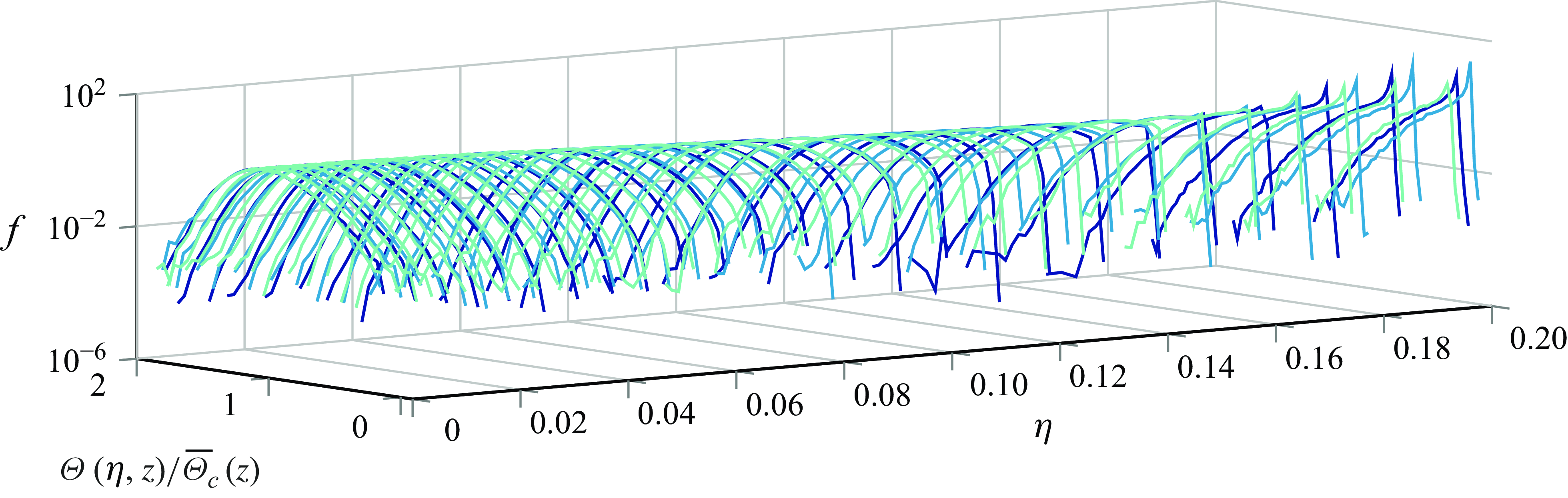
Figure 10 depicts the radial PDF evolution at $z/D=28, 42, 56$
. As
$z/D=28, 42, 56$
. As $\eta$
increases, significant deviations from Gaussian behaviour and the emergence of heavy and skewed tails becomes apparent. The PDF approaches a delta distribution for large
$\eta$
increases, significant deviations from Gaussian behaviour and the emergence of heavy and skewed tails becomes apparent. The PDF approaches a delta distribution for large $\eta$
due to the passive scalar concentration being zero in the ambient region. Additionally, we can extract that the PDFs collapse due to the scaling of
$\eta$
due to the passive scalar concentration being zero in the ambient region. Additionally, we can extract that the PDFs collapse due to the scaling of $\eta$
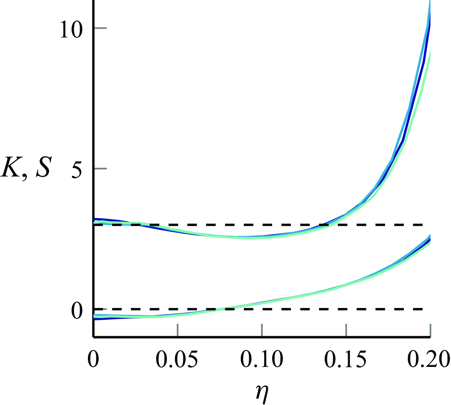
. Quantitative insights from figure 11 show the collapse of skewness
$\eta$
. Quantitative insights from figure 11 show the collapse of skewness $S$
and kurtosis
$S$
and kurtosis $K$
for
$K$
for $z/D=28, 42, 56$
. The Gaussian values,
$z/D=28, 42, 56$
. The Gaussian values, $S=0$
and
$S=0$
and $K=3$
, serve as references. From figure 11 we can also see that the PDF becomes more sub-Gaussian as
$K=3$
, serve as references. From figure 11 we can also see that the PDF becomes more sub-Gaussian as $\eta$
increases. This is consistent with the observations in Birch et al. (Reference Birch, Brown, Dodson and Thomas1978), where the distribution becomes broader with increasing
$\eta$
increases. This is consistent with the observations in Birch et al. (Reference Birch, Brown, Dodson and Thomas1978), where the distribution becomes broader with increasing $\eta$
. This is expected due to intermittent mixing of the turbulent flow in the inner region and the ambient laminar fluid in the outer region. For larger
$\eta$
. This is expected due to intermittent mixing of the turbulent flow in the inner region and the ambient laminar fluid in the outer region. For larger $\eta$
, the mean value of
$\eta$
, the mean value of $\Theta (\eta ,z)/\overline {\Theta }_c(z)$
approaches zero. As a result, the PDF can no longer be approximated by a Gaussian because it would require negative values of
$\Theta (\eta ,z)/\overline {\Theta }_c(z)$
approaches zero. As a result, the PDF can no longer be approximated by a Gaussian because it would require negative values of $\Theta (\eta ,z)/\overline {\Theta }_c(z)$
to maintain a Gaussian distribution. In Birch et al. (Reference Birch, Brown, Dodson and Thomas1978), the distribution becomes bimodal and they interpret this as intermittency in the flow. This is similar to what is observed in figure 12 at
$\Theta (\eta ,z)/\overline {\Theta }_c(z)$
to maintain a Gaussian distribution. In Birch et al. (Reference Birch, Brown, Dodson and Thomas1978), the distribution becomes bimodal and they interpret this as intermittency in the flow. This is similar to what is observed in figure 12 at $\eta =0.139$
for
$\eta =0.139$
for $z/D=28$
. As the distance from the centreline increases to
$z/D=28$
. As the distance from the centreline increases to $\eta =0.149$
, the probability of zero passive scalar concentration quickly becomes dominant.
$\eta =0.149$
, the probability of zero passive scalar concentration quickly becomes dominant.
Kurtosis $K$
(above) and skewness
$K$
(above) and skewness $S$
(below) of
$S$
(below) of $\Theta (\eta ,z)/\overline {\Theta }_{c}(z)$
for
$\Theta (\eta ,z)/\overline {\Theta }_{c}(z)$
for $z/D=28$
(
$z/D=28$
(![]() ),
), $42$
(
$42$
(![]() ),
), $56$
(
$56$
(![]() ). Here,
). Here, $K=3$
,
$K=3$
, $S=0$
(dashed) are the Gaussian values.
$S=0$
(dashed) are the Gaussian values.
Probability density functions of $\Theta (\eta ,z=28)/\overline {\Theta }_{c}(z=28)$
for
$\Theta (\eta ,z=28)/\overline {\Theta }_{c}(z=28)$
for $\eta =0.139$
(solid) and
$\eta =0.139$
(solid) and $\eta =0.149$
(dashed).
$\eta =0.149$
(dashed).
5. Symmetry theory for a passive scalar in a round jet
For a detailed analysis of arbitrary mixed moments, we intend to apply Lie-symmetry analysis to the multi-point velocity–scalar correlation equations (MPVSCEs). The MPVSCEs are a generalisation of the MPMEs and the multi-point scalar equations (MPSEs) and will be derived in the following. Employing Lie-symmetry analysis, we then construct self-similar (group-invariant) solutions i.e. the scaling laws of the passive scalar and the mixed velocity–passive scalar moments and compare them with the DNS data.
5.1. Multi-point correlation equations for passive scalar and velocity moments
In the first step, our goal is to derive the MPSEs and then extend this derivation to the MPVSCEs, which include both the MPMEs and the MPSEs. Similar to the MPMEs, the MPSEs are derived by multiplying (2.4) with $m-1$
passive scalars at
$m-1$
passive scalars at $m-1$
different locations
$m-1$
different locations $\boldsymbol{x}_{(l)}$
followed by statistical averaging. Both the MPSEs and MPVSCEs are an infinite set of linear equations, analogical to the MPMEs. The resulting
$\boldsymbol{x}_{(l)}$
followed by statistical averaging. Both the MPSEs and MPVSCEs are an infinite set of linear equations, analogical to the MPMEs. The resulting $m$
th-order MPSE is expressed as
$m$
th-order MPSE is expressed as
 \begin{equation} \frac {\partial H_{\Theta _{\{m\}}}}{\partial t}+\sum _{l=1}^{m}\left [\frac {\partial }{\partial x_{k_{(l)}}} \left [H_{\Theta _{\{m+1\}}[\Theta _{(m+1)}\mapsto k_{(l)}]}\left [\boldsymbol{x}_{(m+1)}\mapsto \boldsymbol{x}_{(l)}\right ]\right ] -\frac {1}{Pe}\frac {\partial ^{2} H_{\Theta _{\{m\}}}}{\partial x_{k_{(l)}}\partial x_{k_{(l)}}}\right ]=0, \end{equation}
for $m=1,\ldots ,\infty ,$
where
$m=1,\ldots ,\infty ,$
where
 \begin{equation} H_{\Theta _{\{m\}}}=\overline {\Theta (\boldsymbol{x}_{(1)})\Theta (\boldsymbol{x}_{(2)}) \cdot \ldots \cdot \Theta (\boldsymbol{x}_{(m)})}, \end{equation}
and
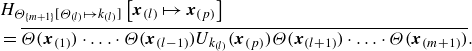 \begin{align} &H_{\Theta _{\{m+1\}}[\Theta _{(l)}\mapsto k_{(l)}]}\left [\boldsymbol{x}_{(l)}\mapsto \boldsymbol{x}_{(p)}\right ]\nonumber \\ & = \overline {\Theta (\boldsymbol{x}_{(1)})\cdot \ldots \cdot \Theta (\boldsymbol{x}_{(l-1)}) U_{k_{(l)}}(\boldsymbol{x}_{(p)})\Theta (\boldsymbol{x}_{(l+1)})\cdot \ldots \cdot \Theta (\boldsymbol{x}_{(m+1)})}. \end{align}
A detailed derivation is available in Appendix A. In a similar approach, the MPVSCEs can be derived with (2.2) and (2.4) giving
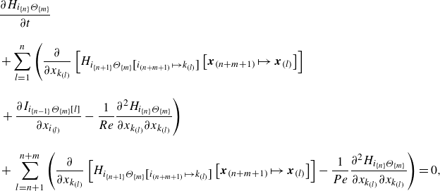 \begin{align} &\frac {\partial H_{i_{\{n\}}\Theta _{\{m\}}}}{\partial t}\nonumber \\[10pt] & + \sum _{l=1}^{n} \left (\frac {\partial }{\partial x_{k_{(l)}}}\left [H_{i_{\{n+1\}}\Theta _{\{m\}}\left [i_{(n+m+1)}\mapsto k_{(l)}\right ]}\left [\boldsymbol{x}_{(n+m+1)}\mapsto \boldsymbol{x}_{(l)} \right ]\right] \right. \nonumber\\[10pt]&\left. +\,\frac {\partial I_{i_{\{n-1\}}\Theta _{\{m\}}\left [ l\right ]}}{\partial x_{i_{(l)}}} -\frac {1}{Re}\frac {\partial ^{2} H_{i_{\{n\}}\Theta _{\{m\}}}}{\partial x_{k_{(l)}} \partial x_{k_{(l)}}}\right )\nonumber \\[10pt] & +\, \sum _{l=n+1}^{n+m} \left (\frac {\partial }{\partial x_{k_{(l)}}}\left [H_{i_{\{n+1\}}\Theta _{\{m\}}\left [i_{(n+m+1)}\mapsto k_{(l)}\right ]}\left [\boldsymbol{x}_{(n+m+1)}\mapsto \boldsymbol{x}_{(l)} \right ]\right ]-\frac {1}{Pe}\frac {\partial ^{2} H_{i_{\{n\}}\Theta _{\{m\}}}}{\partial x_{k_{(l)}} \partial x_{k_{(l)}}}\right )=0, \nonumber\\\end{align}
for $n,m=1,\ldots ,\infty$
, where
$n,m=1,\ldots ,\infty$
, where
 \begin{equation} H_{i_{\{n\}}\Theta _{\{m\}}}=\overline {U_{i_{(1)}}(\boldsymbol{x}_{(1)})\cdot \ldots \cdot U_{i_{(n)}}(\boldsymbol{x}_{(n)})\Theta (\boldsymbol{x}_{(n+1)}) \cdot \ldots \cdot \Theta (\boldsymbol{x}_{(n+m)})} ,\end{equation}
and the pressure correlation term is defined as
 \begin{equation} I_{i_{\{n-1\}}\Theta _{\{m\}}\left [ l\right ]}= \overline {U_{i_{(1)}}(\boldsymbol{x}_{(1)}) \cdot \ldots \cdot P(\boldsymbol{x}_{(l)}) \cdot \ldots \cdot U_{i_{(n)}}(\boldsymbol{x}_{(n)})\Theta (\boldsymbol{x}_{(n+1)}) \cdot \ldots \cdot \Theta (\boldsymbol{x}_{(n+m)})}. \end{equation}
More details about the derivation can be found in Appendix B. Setting $m=0$
yields the MPMEs from (5.4), while
$m=0$
yields the MPMEs from (5.4), while $n=0$
yields the MPSEs. The MPVSCEs (5.4) are a set of linear differential equations, a crucial feature for the occurrence of the two statistical symmetries (Wacławczyk et al. Reference Wacławczyk, Staffolani, Oberlack, Rosteck, Wilczek and Friedrich2014) to be used below.
$n=0$
yields the MPSEs. The MPVSCEs (5.4) are a set of linear differential equations, a crucial feature for the occurrence of the two statistical symmetries (Wacławczyk et al. Reference Wacławczyk, Staffolani, Oberlack, Rosteck, Wilczek and Friedrich2014) to be used below.
5.2. Symmetry-based scaling laws for a passive scalar
The methodology of Lie-symmetry analysis uses continuous transformation groups to unify methods for solving differential equations and finds applications in various fields of applied mathematics and theoretical physics. For a comprehensive understanding, see Bluman, Cheviakov & Anco (Reference Bluman, Cheviakov and Anco2010). In the following, the concept of symmetries of differential equations is briefly introduced. Symmetries in differential equations are transformations that leave the form of the equations unchanged. Consider a system of partial differential equations
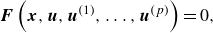 \begin{equation} \boldsymbol{F}\left (\boldsymbol{x}, \boldsymbol{u}, \boldsymbol{u}^{(1)}, \ldots ,\boldsymbol{u}^{(p)}\right )=0, \end{equation}
with a transformation
 \begin{equation} \boldsymbol{x}^{*} = \boldsymbol{\phi }(\boldsymbol{x},\boldsymbol{u};a), \quad \boldsymbol{u}^{*} = \boldsymbol{\psi }(\boldsymbol{x},\boldsymbol{u};a), \end{equation}
where $\boldsymbol{x}$
,
$\boldsymbol{x}$
, $\boldsymbol{u}$
,
$\boldsymbol{u}$
, $a$
are the independent variables, dependent variables and an arbitrary continuous parameter
$a$
are the independent variables, dependent variables and an arbitrary continuous parameter $a \in \mathbb{R}$
, respectively. The transformation is considered a symmetry transformation if
$a \in \mathbb{R}$
, respectively. The transformation is considered a symmetry transformation if
 \begin{equation} \boldsymbol{F}\left (\boldsymbol{x}, \boldsymbol{u}, \boldsymbol{u}^{(1)}, \ldots ,\boldsymbol{u}^{(p)}\right )=0 \iff \boldsymbol{F}\left (\boldsymbol{x}^{*}, \boldsymbol{u}^{*}, \boldsymbol{u}^{*(1)}, \ldots ,\boldsymbol{u}^{*(p)}\right )=0, \end{equation}
where $\boldsymbol{u}^{(p)}$
refers to the
$\boldsymbol{u}^{(p)}$
refers to the $p$
th derivative of
$p$
th derivative of $\boldsymbol{u}$
. In this case, we consider (2.2) with
$\boldsymbol{u}$
. In this case, we consider (2.2) with $Re^{-1}=0$
, which admits the following two-parameter symmetry:
$Re^{-1}=0$
, which admits the following two-parameter symmetry:
 \begin{equation} t^\ast = \textrm { e}^{a_{St}} t, \thinspace \boldsymbol{x}^\ast = \textrm { e}^{a_{Sx}} \boldsymbol{x}, \thinspace \boldsymbol{U}^\ast = \textrm { e}^{a_{Sx}-a_{St}} \boldsymbol{U}, \thinspace P^\ast = \textrm { e}^{2(a_{Sx}-a_{St})} P, \thinspace a_{Sx},a_{St}\in \mathbb{R} . \end{equation}
If we now insert (5.10) into (2.2) under the frictionless assumption, we find the prefactor $\textrm { e}^{2a_{St}-a_{Sx}}$
in front of each of the three terms, which can be cancelled out, and we get
$\textrm { e}^{2a_{St}-a_{Sx}}$
in front of each of the three terms, which can be cancelled out, and we get $({(\partial \boldsymbol{U}^\ast )}/{(\partial \boldsymbol{U}{t^\ast})}) + (\boldsymbol{U}^\ast \cdot \nabla ^\ast ) \boldsymbol{U}^\ast = - \nabla ^\ast P^\ast$
. This proves the scaling symmetry. Two things are important for the following analyses: (i) the scaling symmetries of (2.2) but also (2.4) transfer to the moment equations; (ii) the scaling symmetry of time characterised by the group parameter
$({(\partial \boldsymbol{U}^\ast )}/{(\partial \boldsymbol{U}{t^\ast})}) + (\boldsymbol{U}^\ast \cdot \nabla ^\ast ) \boldsymbol{U}^\ast = - \nabla ^\ast P^\ast$
. This proves the scaling symmetry. Two things are important for the following analyses: (i) the scaling symmetries of (2.2) but also (2.4) transfer to the moment equations; (ii) the scaling symmetry of time characterised by the group parameter $a_{St}$
is preserved for the stationary case of the Euler equation, because the above-mentioned scaling factor does not change for this case, even if the unsteady term is no longer included. This also remains the case if one considers a statistically stationary flow for the present case, because the key variables such as velocity
$a_{St}$
is preserved for the stationary case of the Euler equation, because the above-mentioned scaling factor does not change for this case, even if the unsteady term is no longer included. This also remains the case if one considers a statistically stationary flow for the present case, because the key variables such as velocity $\boldsymbol{U}$
and pressure
$\boldsymbol{U}$
and pressure $P$
apparently also contain time as a basic variable, and this applies equally to the corresponding statistical moments.
$P$
apparently also contain time as a basic variable, and this applies equally to the corresponding statistical moments.
The following set of selected symmetries are relevant for the derivation of the scaling laws of a turbulent round jet, which have their origin in the NSEs and the passive scalar equations. In the limit of $Re \to \infty$
they are transferred to the H-approach, which consist of a translation symmetry in space
$Re \to \infty$
they are transferred to the H-approach, which consist of a translation symmetry in space
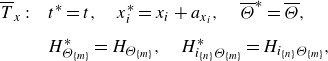 \begin{align} \overline {T}_{x}: \quad &t^{*}=t, \quad {x}^{*}_i={x}_i+a_{x_i},\quad \overline {\Theta }^{*}= \overline {\Theta }, \nonumber \\[6pt] & H^{*}_{\Theta _{\{m\}}}=H_{\Theta _{\{m\}}},\quad H^{*}_{i_{\{n\}}\Theta _{\{m\}}}=H_{i_{\{n\}}\Theta _{\{m\}}}, \end{align}
and a scaling symmetry in space ( $a_{Sx}$
), time (
$a_{Sx}$
), time ( $a_{St}$
) and of the passive scalar (
$a_{St}$
) and of the passive scalar ( $a_{S\theta }$
)
$a_{S\theta }$
)
 \begin{align} & \overline {T}_{S}: \quad t^{*}=\mathrm{e}^{a_{St}}t, \quad {x}^{*}_i=\mathrm{e}^{a_{Sx}}{x}_i,\quad \overline {\Theta }^{*}=\mathrm{e}^{a_{S\theta }} \overline {\Theta }, \nonumber \\[6pt] & H^{*}_{\Theta _{\{m\}}}=\mathrm{e}^{m a_{S\theta }} H_{\Theta _{\{m\}}},\quad H^{*}_{i_{\{n\}}\Theta _{\{m\}}}=\mathrm{e}^{ma_{S\theta }+n(a_{Sx}-a_{St})}H_{i_{\{n\}}\Theta _{\{m\}}}. \end{align}
It is noteworthy that the NSEs exhibit a restricted set of scaling symmetries compared with the Euler equations, in particular $a_{St} = 2a_{Sx}$
in the symmetry above which can be shown by substituting the scaling symmetry (5.10) into the NSEs. For turbulent flows at higher
$a_{St} = 2a_{Sx}$
in the symmetry above which can be shown by substituting the scaling symmetry (5.10) into the NSEs. For turbulent flows at higher $Re$
, viscosity dominates only on length scales between the Taylor and the Kolmogorov length scales or the corresponding wavenumbers in spectral space. This is supported by Oberlack (Reference Oberlack2000), where a boundary layer type of asymptotic expansion was performed in correlation space. As a result, the multi-point equations for turbulent flows for large scales admit the scaling symmetries of the inviscid form of the equation and, hence, to leading order, no
$Re$
, viscosity dominates only on length scales between the Taylor and the Kolmogorov length scales or the corresponding wavenumbers in spectral space. This is supported by Oberlack (Reference Oberlack2000), where a boundary layer type of asymptotic expansion was performed in correlation space. As a result, the multi-point equations for turbulent flows for large scales admit the scaling symmetries of the inviscid form of the equation and, hence, to leading order, no $Re$
dependence is implied. In full analogy, this can also be shown for the
$Re$
dependence is implied. In full analogy, this can also be shown for the $Pe$
number dependence. Additionally, a statistical symmetry on the basis of the linear MPVSCEs in (5.4) is considered
$Pe$
number dependence. Additionally, a statistical symmetry on the basis of the linear MPVSCEs in (5.4) is considered
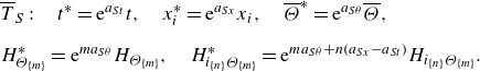
 \begin{align} \overline {T}_{Ss}: \quad &t^{*}=t, \quad {x}^{*}_i={x}_i,\quad \overline {\Theta }^{*}=\mathrm{e}^{a_{Ss}} \overline {\Theta }, \\[6pt] & H^{*}_{\Theta _{\{m\}}}=\mathrm{e}^{a_{Ss}} H_{\Theta _{\{m\}}},\quad H^{*}_{i_{\{n\}}\Theta _{\{m\}}}=\mathrm{e}^{a_{Ss}}H_{i_{\{n\}}\Theta _{\{m\}}},\nonumber \end{align}
which is a measure of intermittency. In Wacławczyk et al. (Reference Wacławczyk, Staffolani, Oberlack, Rosteck, Wilczek and Friedrich2014) this has been concluded by analysing the PDF formulation of the moment equation known as the Lundgren–Monin–Novikov hierarchy. In this formulation, the group parameter $a_{Ss}$
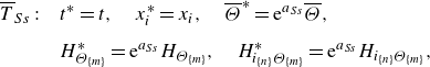
of an equivalent symmetry scales the shape of a PDF such that intermittency is characterised. This so-called intermittency symmetry does not appear in either the NSEs or the passive scalar equation. For the linear systems (5.1)–(5.6), there exists also the generic symmetry of superposition, which does not play a role in the present subsection, however, and only comes into play in §§ 5.4. The combination of the symmetries (5.11)–(5.13) leads to the characteristic condition for the invariant solution, i.e. turbulent scaling laws of the velocity and passive scalar moments of a spatially evolving turbulent round jet. Although the system (5.1)–(5.6) constitutes an arbitrary multi-point moments hierarchy, in the following, we will only consider one-point statistics and scaling laws, i.e.
$a_{Ss}$
of an equivalent symmetry scales the shape of a PDF such that intermittency is characterised. This so-called intermittency symmetry does not appear in either the NSEs or the passive scalar equation. For the linear systems (5.1)–(5.6), there exists also the generic symmetry of superposition, which does not play a role in the present subsection, however, and only comes into play in §§ 5.4. The combination of the symmetries (5.11)–(5.13) leads to the characteristic condition for the invariant solution, i.e. turbulent scaling laws of the velocity and passive scalar moments of a spatially evolving turbulent round jet. Although the system (5.1)–(5.6) constitutes an arbitrary multi-point moments hierarchy, in the following, we will only consider one-point statistics and scaling laws, i.e. $\boldsymbol{x}_{(1)}=\boldsymbol{x}_{(2)}=\ldots =\boldsymbol{x}_{(n+m)}$
and therefore
$\boldsymbol{x}_{(1)}=\boldsymbol{x}_{(2)}=\ldots =\boldsymbol{x}_{(n+m)}$
and therefore $H_{i_{\{n\}}\Theta _{\{m\}}}=\overline {U^n_{[i]}\Theta ^m}$
, where
$H_{i_{\{n\}}\Theta _{\{m\}}}=\overline {U^n_{[i]}\Theta ^m}$
, where $[\,\cdot \,]$
means that no summation is implied. The related characteristic condition reads
$[\,\cdot \,]$
means that no summation is implied. The related characteristic condition reads
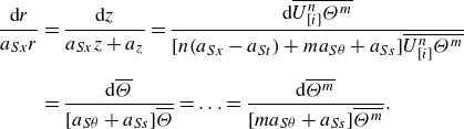 \begin{align} \frac {\mathrm{d}r}{a_{Sx}r}&=\frac {\mathrm{d}z}{a_{Sx}z+a{_{z}}}=\frac {\mathrm{d}\overline {U_{[i]}^{n} \Theta ^m}}{[n(a_{Sx}-a_{St})+ma_{S\theta }+a_{Ss}]\overline {U_{[i]}^n \Theta ^m}}\nonumber \\[6pt] &=\frac {\mathrm{d}\overline {\Theta }}{[a_{S\theta }+a_{Ss}]\overline {\Theta }}=\ldots =\frac {\mathrm{d}\overline {\Theta ^m}}{[ma_{S\theta }+a_{Ss}]\overline {\Theta ^m}}. \end{align}
Symmetry breaking is introduced through flow-specific invariants for the turbulent jet, i.e. the thermal energy conservation (Sadeghi, Oberlack & Gauding Reference Sadeghi, Oberlack and Gauding2021)
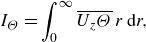 \begin{equation} I_\Theta =\int _{0}^\infty \overline {U_z \Theta }\,r\,\mathrm{d}r ,\end{equation}
and the generalised momentum integral as derived in Nguyen & Oberlack (Reference Nguyen and Oberlack2024b )
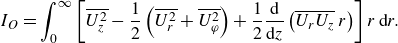 \begin{equation} I_O=\int _0^\infty \left [ \overline {U_z^{2}}-\frac {1}{2}\left (\overline {U_r^{2}}+\overline {U_\varphi ^{2}}\right )+\frac {1}{2} \frac {\mathrm{d}}{\mathrm{d}z} \left (\overline {U_rU_z}\,r\right )\right ]r\,\mathrm{d}r .\end{equation}
The group parameters of the symmetries are constrained through these invariants. The symmetry breaking is induced by implementing the symmetries (5.11)–(5.13) in (5.15) through $\overline {U_z \Theta }=\mathrm{e}^{-(a_{S\theta }+a_{Sx}-a_{St}+a_{Ss})}\overline {U_z \Theta }^{*}$
and
$\overline {U_z \Theta }=\mathrm{e}^{-(a_{S\theta }+a_{Sx}-a_{St}+a_{Ss})}\overline {U_z \Theta }^{*}$
and $r=\mathrm{e}^{-a_{Sx}}r^{*}$
, which gives
$r=\mathrm{e}^{-a_{Sx}}r^{*}$
, which gives
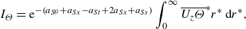 \begin{equation} I_\Theta =\mathrm{e}^{-(a_{S\theta }+a_{Sx}-a_{St}+2a_{Sx}+a_{Ss})} \int _{0}^\infty \overline {U_z \Theta }^{*}r^{*}\,\mathrm{d}r^{*}, \end{equation}
and in (5.16) through $\overline {U^{2}_{i}}=\mathrm{e}^{-2(a_{Sx}-a_{St})-a_{Ss}}\overline {U^{2}_{i}}^{*}$
and
$\overline {U^{2}_{i}}=\mathrm{e}^{-2(a_{Sx}-a_{St})-a_{Ss}}\overline {U^{2}_{i}}^{*}$
and $\overline {U_{i}}^{*}=\mathrm{e}^{-(a_{Sx}-a_{St})-a_{Ss}}\overline {U_{i}}^{*}$
, we obtain
$\overline {U_{i}}^{*}=\mathrm{e}^{-(a_{Sx}-a_{St})-a_{Ss}}\overline {U_{i}}^{*}$
, we obtain
 \begin{equation} I_O= \mathrm{e}^{-4a_{Sx}+2a_{St}-a_{Ss}}\int _0^\infty \left [ \overline {U_z^{2}}^{*}-\frac {1}{2}\left (\overline {U_r^{2}}^{*}+\overline {U_\varphi ^{2}}^{*}\right ) +\frac {1}{2} \frac {\mathrm{d}}{\mathrm{d}z^{*}} \left (\overline {U_rU_z}^{*}r^{*}\right )\right ]r^{*}\mathrm{d}r^{*}. \end{equation}
Inferring $I_\Theta$
and
$I_\Theta$
and $I_O$
are invariants, i.e. constants, results in the symmetry breaking
$I_O$
are invariants, i.e. constants, results in the symmetry breaking $a_{S\theta }+3a_{Sx}-a_{St}+a_{Ss}=0$
and
$a_{S\theta }+3a_{Sx}-a_{St}+a_{Ss}=0$
and $4a_{Sx}-2a_{St}+a_{Ss}=0$
to maintain invariance. When solved for
$4a_{Sx}-2a_{St}+a_{Ss}=0$
to maintain invariance. When solved for $a_{St}$
and
$a_{St}$
and $a_{S\theta }$
, we find
$a_{S\theta }$
, we find
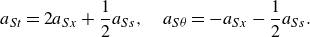 \begin{equation} a_{St}=2a_{Sx}+\frac {1}{2}a_{Ss}, \quad a_{S\theta }=-a_{Sx}-\frac {1}{2}a_{Ss}. \end{equation}
Under the consideration of the symmetry breaking (5.19), the turbulent scaling laws can be derived by integrating the characteristic condition in (5.14)
 \begin{align} \eta &=\frac {r}{z-z_0} ,\end{align}
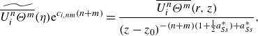 \begin{align} \widetilde {\overline {U_i^n\Theta ^m}}(\eta )\mathrm{e}^{c_{i,nm}(n+m)}&= \displaystyle\frac {\overline {U_i^n\Theta ^m}(r,z)}{(z-z_0)^{-(n+m)(1+\frac {1}{2}a_{Ss}^{*})+a_{Ss}^{*}}} ,\end{align}
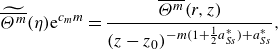 \begin{align} \widetilde {\overline {\Theta ^m}}(\eta )\mathrm{e}^{c_{m}m}&=\displaystyle\frac {\overline {\Theta ^m}(r,z)}{(z-z_0)^{-m(1+\frac {1}{2}a_{Ss}^{*})+a_{Ss}^{*}}}, \end{align}
where $z_0 = -a_z /a_{Sx}$
is the virtual origin and
$z_0 = -a_z /a_{Sx}$
is the virtual origin and $a_{Ss}^{*}=a_{Ss}/a_{Sx}$
. The variables marked with
$a_{Ss}^{*}=a_{Ss}/a_{Sx}$
. The variables marked with $\widetilde {(\,\cdot \,)}$
are the invariants i.e. the similarity variables.
$\widetilde {(\,\cdot \,)}$
are the invariants i.e. the similarity variables.
In Nguyen & Oberlack (Reference Nguyen and Oberlack2024b
), we found that the statistical symmetry (5.13), giving a measure of intermittency (Wacławczyk et al. Reference Wacławczyk, Staffolani, Oberlack, Rosteck, Wilczek and Friedrich2014), allows for a possible variation of the turbulent decay behaviour of the moments in the $z$
-direction agreeing with the hypothesis of George (Reference George1989). However, this observation stands despite the present DNS data showing that, for the intermittency symmetry (5.13), we have
$z$
-direction agreeing with the hypothesis of George (Reference George1989). However, this observation stands despite the present DNS data showing that, for the intermittency symmetry (5.13), we have $a_{Ss}=0$
. Nevertheless, the intermittency reappears in the reduced equations of the MPMEs through the scaling laws. Subsequently, it is shown that this also applies to passive scalars as detailed in § 5.4.
$a_{Ss}=0$
. Nevertheless, the intermittency reappears in the reduced equations of the MPMEs through the scaling laws. Subsequently, it is shown that this also applies to passive scalars as detailed in § 5.4.
The invariant $\eta$
is received by integrating the first two terms of (5.14) and (5.21) results in the integration of the second and third terms and finally (5.22) emerges after integrating the second and the remaining terms in (5.14). The integration constants
$\eta$
is received by integrating the first two terms of (5.14) and (5.21) results in the integration of the second and third terms and finally (5.22) emerges after integrating the second and the remaining terms in (5.14). The integration constants $c_{i,nm}$
and
$c_{i,nm}$
and $c_{m}$
emerge from the integration and move into the exponent after exponentiation. From (5.21), we see not only the turbulent scaling law of the mixed moments but also a generalisation of the velocity and passive scalar scaling laws. For
$c_{m}$
emerge from the integration and move into the exponent after exponentiation. From (5.21), we see not only the turbulent scaling law of the mixed moments but also a generalisation of the velocity and passive scalar scaling laws. For $m=0$
, the velocity scaling laws are received as derived in Nguyen & Oberlack (Reference Nguyen and Oberlack2024b
), while for
$m=0$
, the velocity scaling laws are received as derived in Nguyen & Oberlack (Reference Nguyen and Oberlack2024b
), while for $n=0$
we obtain the passive scalar scaling law (5.22).
$n=0$
we obtain the passive scalar scaling law (5.22).
5.3. Validation of the scaling laws
Just as in Nguyen & Oberlack (Reference Nguyen and Oberlack2024b
), $a^\ast _{Ss}$
generates a one-parameter family of scaling laws which, as conjectured by George (Reference George1989), may be induced by a variation of the inflow condition. However, the purely hydrodynamic turbulence DNS in Nguyen & Oberlack (Reference Nguyen and Oberlack2024b
) has already shown that
$a^\ast _{Ss}$
generates a one-parameter family of scaling laws which, as conjectured by George (Reference George1989), may be induced by a variation of the inflow condition. However, the purely hydrodynamic turbulence DNS in Nguyen & Oberlack (Reference Nguyen and Oberlack2024b
) has already shown that $a^\ast _{Ss}=0$
and we find this result confirmed by the coupling of the NSEs (2.1) and (2.2) with the scalar equation (2.4). Furthermore, it can be inferred that
$a^\ast _{Ss}=0$
and we find this result confirmed by the coupling of the NSEs (2.1) and (2.2) with the scalar equation (2.4). Furthermore, it can be inferred that $a^\ast _{Ss}$
does not differ for the passive scalar scaling law compared with the velocity scaling law. As
$a^\ast _{Ss}$
does not differ for the passive scalar scaling law compared with the velocity scaling law. As $a_{Ss}^{*}=0$
is dependent on the velocity field and also appears in the mixed velocity–scalar moments, the passive scalar cannot have an effect on
$a_{Ss}^{*}=0$
is dependent on the velocity field and also appears in the mixed velocity–scalar moments, the passive scalar cannot have an effect on $a_{Ss}^{*}$
. Physically, this makes sense, since a passive scalar has no effect on the velocity field.
$a_{Ss}^{*}$
. Physically, this makes sense, since a passive scalar has no effect on the velocity field.
The validation of the scaling laws (5.20)–(5.22) is first conducted on the centreline, where $r=0$
. To facilitate a comparison with the DNS results, the scaling laws presented in (5.21) and (5.22) are expressed as
$r=0$
. To facilitate a comparison with the DNS results, the scaling laws presented in (5.21) and (5.22) are expressed as
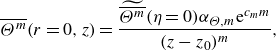 \begin{equation} \overline {\Theta ^m}(r=0,z)=\frac {\widetilde {\overline {\Theta ^m}}(\eta =0)\alpha _{\Theta ,m}\mathrm{e}^{c_m m}}{(z-z_0)^{m}}, \end{equation}
where $\alpha _{\Theta ,m}$
is extracted so that
$\alpha _{\Theta ,m}$
is extracted so that $\widetilde {\overline {\Theta ^m}}(\eta =0)=1$
and
$\widetilde {\overline {\Theta ^m}}(\eta =0)=1$
and
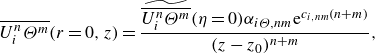 \begin{equation} \overline {U_{i}^n\Theta ^m}(r=0,z)=\frac {\widetilde {\overline {U_{i}^n\Theta ^m}}(\eta =0)\alpha _{i\Theta ,nm}\mathrm{e}^{c_{i,nm} (n+m)}}{(z-z_0)^{n+m}}, \end{equation}
where we again extract $\alpha _{i\Theta ,nm}$
so that the invariant
$\alpha _{i\Theta ,nm}$
so that the invariant $\widetilde {\overline {U_{i}^n\Theta ^m}}(\eta =0)=1$
. These formulations allow for a direct comparison between the scaling laws and the DNS data at the centreline.
$\widetilde {\overline {U_{i}^n\Theta ^m}}(\eta =0)=1$
. These formulations allow for a direct comparison between the scaling laws and the DNS data at the centreline.
Analysing the DNS data shown in figure 13, we conclude that for $n=0$
we obtain
$n=0$
we obtain $c_m=c=1.755$
and
$c_m=c=1.755$
and $\alpha _{\Theta ,m}=\alpha _{\Theta }=0.722$
for the purely passive scalar scaling (5.22). Note that both constants are independent of the moment order
$\alpha _{\Theta ,m}=\alpha _{\Theta }=0.722$
for the purely passive scalar scaling (5.22). Note that both constants are independent of the moment order $m$
. This implies that
$m$
. This implies that $c$
is an invariant with respect to
$c$
is an invariant with respect to $m$
. So far, this cannot be derived directly from symmetry theory, but support is essentially from the DNS data.
$m$
. So far, this cannot be derived directly from symmetry theory, but support is essentially from the DNS data.
Extending this to the scaling law of the mixed moments for $i=z$
in (5.24), it can be observed that the constants in figure 13 span a plane. For
$i=z$
in (5.24), it can be observed that the constants in figure 13 span a plane. For $i=r,\varphi$
, a ‘discrete’ plane is formed because the moments are zero for odd
$i=r,\varphi$
, a ‘discrete’ plane is formed because the moments are zero for odd $n$
on the centreline in figure 14. This results, as explained in Nguyen & Oberlack (Reference Nguyen and Oberlack2024b
), from the fact that the pure velocity scaling law for
$n$
on the centreline in figure 14. This results, as explained in Nguyen & Oberlack (Reference Nguyen and Oberlack2024b
), from the fact that the pure velocity scaling law for $i=r,\varphi$
(
$i=r,\varphi$
( $m=0$
) is described by a centred Gaussian process. Since the analysis is performed on the centreline, the scaling law (5.24) gives the same values for
$m=0$
) is described by a centred Gaussian process. Since the analysis is performed on the centreline, the scaling law (5.24) gives the same values for $i=r,\varphi$
due to symmetry. Therefore, only
$i=r,\varphi$
due to symmetry. Therefore, only $i=r$
will be considered in the following. The prefactors of the scaling law in (5.24) can be characterised by an arithmetic weighing of the moments with
$i=r$
will be considered in the following. The prefactors of the scaling law in (5.24) can be characterised by an arithmetic weighing of the moments with
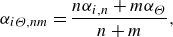 \begin{equation} \alpha _{i\Theta ,nm}=\frac {n \alpha _{i,n}+m\alpha _\Theta }{n+m}, \end{equation}
and
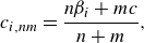 \begin{equation} c_{i,nm}=\frac {n\beta _i+m c}{n+m}, \end{equation}
where $\alpha _{z,n}=\alpha _z=0.673$
,
$\alpha _{z,n}=\alpha _z=0.673$
, $\beta _z=2.123$
,
$\beta _z=2.123$
, $\alpha _{r,n}=\sqrt {2\mathrm{e}}\ [1.81(n-1) ]^{{n}/{2}}$
and
$\alpha _{r,n}=\sqrt {2\mathrm{e}}\ [1.81(n-1) ]^{{n}/{2}}$
and $\beta _r=-0.5$
are taken from Nguyen & Oberlack (Reference Nguyen and Oberlack2024b
).
$\beta _r=-0.5$
are taken from Nguyen & Oberlack (Reference Nguyen and Oberlack2024b
).
The exponential prefactor $\alpha _{z\Theta ,nm}\mathrm{e}^{c_{z,nm} (n+m)}$
(
$\alpha _{z\Theta ,nm}\mathrm{e}^{c_{z,nm} (n+m)}$
(![]() ) from (5.24) determined with the DNS data for mixed moments up to
) from (5.24) determined with the DNS data for mixed moments up to $n+m=6$
(
$n+m=6$
(![]() ), for
), for $\Theta$
moments up to
$\Theta$
moments up to $m=10$
(
$m=10$
(![]() ) and
) and $U_z$
moments up to
$U_z$
moments up to $n=10$
(
$n=10$
(![]() ) is shown. Additionally, (5.24) is highlighted for
) is shown. Additionally, (5.24) is highlighted for $m=0$
(
$m=0$
(![]() ) and
) and $n=0$
(
$n=0$
(![]() ).
).

The exponential prefactor $\alpha _{r\Theta ,nm}\mathrm{e}^{c_{r,nm} (n+m)}$
(
$\alpha _{r\Theta ,nm}\mathrm{e}^{c_{r,nm} (n+m)}$
(![]() ) from (5.24) determined with the DNS data for mixed moments up to
) from (5.24) determined with the DNS data for mixed moments up to $n+m=6$
(
$n+m=6$
(![]() ), for
), for $\Theta$
moments up to
$\Theta$
moments up to $m=10$
(
$m=10$
(![]() ) and
) and $U_r$
moments up to
$U_r$
moments up to $n=10$
(
$n=10$
(![]() ) is shown. Additionally, (5.24) is highlighted for
) is shown. Additionally, (5.24) is highlighted for $m=0$
(
$m=0$
(![]() ) and
) and $n=0$
(
$n=0$
(![]() ).
).
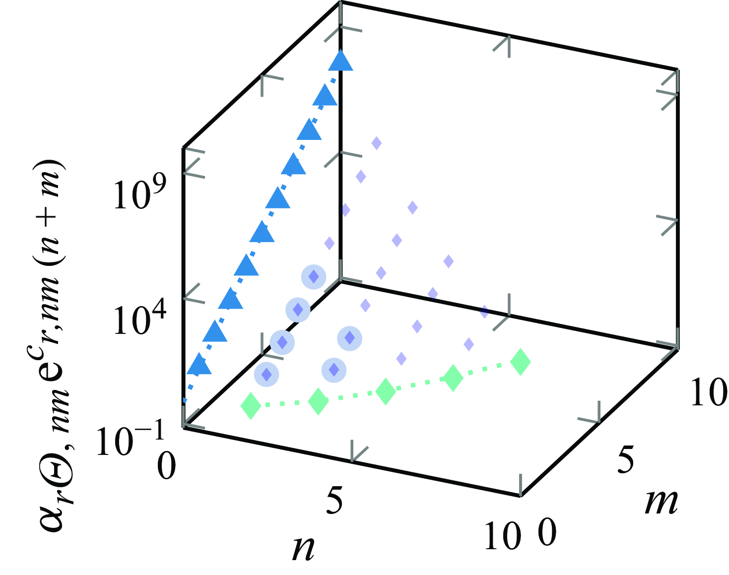
5.4. Gaussian behaviour of the higher passive scalar moments
Interestingly, the passive scalar moments behave similarly to the axial velocity moments. The higher instantaneous $H$
-moments of the passive scalar exhibit a Gaussian-like behaviour in
$H$
-moments of the passive scalar exhibit a Gaussian-like behaviour in $\eta$
, similar to what is observed for the axial velocity moments. By analysing the scaled higher moments of the passive scalar according to (5.22), we find that a Gaussian function provides a highly accurate representation for these moments. The Gaussian function is expressed as
$\eta$
, similar to what is observed for the axial velocity moments. By analysing the scaled higher moments of the passive scalar according to (5.22), we find that a Gaussian function provides a highly accurate representation for these moments. The Gaussian function is expressed as
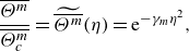 \begin{equation} \frac {\overline {\Theta ^m}}{\overline {\Theta ^m_c}}=\widetilde {\overline {\Theta ^m}}(\eta )=\mathrm{e}^{-\gamma _m \eta ^{2}}, \end{equation}
where $\eta$
represents the dimensionless radial coordinate as defined in (5.20). This Gaussian function captures the characteristic distribution of the passive scalar, showing a rapid decrease in amplitude as the distance from the central region increases. One consequence of representing moments in its
$\eta$
represents the dimensionless radial coordinate as defined in (5.20). This Gaussian function captures the characteristic distribution of the passive scalar, showing a rapid decrease in amplitude as the distance from the central region increases. One consequence of representing moments in its $H$
form is the dominance of the mean over the fluctuations
$H$
form is the dominance of the mean over the fluctuations $R$
. While it may be tempting to assume
$R$
. While it may be tempting to assume $\overline {\Theta ^m}\approx \overline {\Theta }^m$
, implying that
$\overline {\Theta ^m}\approx \overline {\Theta }^m$
, implying that $\gamma _m$
is linear and thus trivial due to the strong dominance of the mean passive scalar concentration
$\gamma _m$
is linear and thus trivial due to the strong dominance of the mean passive scalar concentration $\overline {\Theta }$
over the fluctuations, our analysis demonstrates that
$\overline {\Theta }$
over the fluctuations, our analysis demonstrates that $\gamma _m$
does not behave linearly for larger moments, as is already implied by figure 3 for
$\gamma _m$
does not behave linearly for larger moments, as is already implied by figure 3 for $R_{\Theta \Theta }$
. Employing (5.27) in (1.4), we find that only for
$R_{\Theta \Theta }$
. Employing (5.27) in (1.4), we find that only for $\gamma _2=2 \gamma _1$
could the Gaussian curve be factored out. For this reason, the higher moments of the fluctuations do not have a simple relationship, e.g.
$\gamma _2=2 \gamma _1$
could the Gaussian curve be factored out. For this reason, the higher moments of the fluctuations do not have a simple relationship, e.g. $R_{\Theta \Theta }$
has an off-axis peak (see figure 3) instead of behaving like a Gaussian curve. In figure 15, we observe the self-preservation of six selected moments of the passive scalar, ranging up to order ten, at multiple stages along the spatial domain (
$R_{\Theta \Theta }$
has an off-axis peak (see figure 3) instead of behaving like a Gaussian curve. In figure 15, we observe the self-preservation of six selected moments of the passive scalar, ranging up to order ten, at multiple stages along the spatial domain ( $z/D=25{-}55$
). Except for the central region, there is a collapse of the data when normalised using the scaling law described in (5.23). This collapse suggests a universal scaling behaviour for the moments of the passive scalar, reinforcing the idea of self-preservation. Additionally, the Gaussian-like curves become progressively narrower as the moment order increases. The DNS data up to the tenth axial moment are presented in semi-log scaling in figure 16, demonstrating a parabolic trend, suggesting a strong agreement with (5.27), although the specific value of
$z/D=25{-}55$
). Except for the central region, there is a collapse of the data when normalised using the scaling law described in (5.23). This collapse suggests a universal scaling behaviour for the moments of the passive scalar, reinforcing the idea of self-preservation. Additionally, the Gaussian-like curves become progressively narrower as the moment order increases. The DNS data up to the tenth axial moment are presented in semi-log scaling in figure 16, demonstrating a parabolic trend, suggesting a strong agreement with (5.27), although the specific value of $\gamma _m$
remains undetermined. The deviation of the DNS data from the parabolic curve at the edge is likely attributed to external intermittency, as seen in figure 10. Further,
$\gamma _m$
remains undetermined. The deviation of the DNS data from the parabolic curve at the edge is likely attributed to external intermittency, as seen in figure 10. Further, $\overline {\Theta }^m$
is shown for
$\overline {\Theta }^m$
is shown for $m=2$
to
$m=2$
to $m=10$
, i.e.
$m=10$
, i.e. $\gamma _m=m\gamma _1$
, where the discrepancy discloses that
$\gamma _m=m\gamma _1$
, where the discrepancy discloses that $\gamma _m$
is indeed nonlinear. A comparison between figures 15 and 16 reveals that the turbulent scaling laws hold true within the fully turbulent regime. It is important to note that turbulent scaling laws are usually only valid within the confines of a fully turbulent regime and become less applicable as we move into the ambient environment. The estimation of
$\gamma _m$
is indeed nonlinear. A comparison between figures 15 and 16 reveals that the turbulent scaling laws hold true within the fully turbulent regime. It is important to note that turbulent scaling laws are usually only valid within the confines of a fully turbulent regime and become less applicable as we move into the ambient environment. The estimation of $\gamma _m$
in
$\gamma _m$
in $m$
for the passive scalar moments can be obtained from figure 17 through a straightforward nonlinear fitting procedure. The resulting fit yields
$m$
for the passive scalar moments can be obtained from figure 17 through a straightforward nonlinear fitting procedure. The resulting fit yields
 \begin{equation} \gamma _m=-1.27m^{2} + 37.52m + 27.34, \end{equation}
with a coefficient of determination of $R^{2}=0.99$
, clearly showing that
$R^{2}=0.99$
, clearly showing that $\overline {\Theta ^m}\not \approx \overline {\Theta }^m$
and therefore strong non-Gaussian fluctuations and hence higher moments in general cannot be ignored. In the present DNS
$\overline {\Theta ^m}\not \approx \overline {\Theta }^m$
and therefore strong non-Gaussian fluctuations and hence higher moments in general cannot be ignored. In the present DNS $\gamma _1=73.59$
agrees well with the experiment by Birch et al. (Reference Birch, Brown, Dodson and Thomas1978) at
$\gamma _1=73.59$
agrees well with the experiment by Birch et al. (Reference Birch, Brown, Dodson and Thomas1978) at $\gamma _1=73.6$
. Lubbers et al. (Reference Lubbers, Brethouwer and Boersma2001) found
$\gamma _1=73.6$
. Lubbers et al. (Reference Lubbers, Brethouwer and Boersma2001) found $\gamma _1=59.1$
, which means a wider passive scalar profile. It is interesting to note that Birch et al. (Reference Birch, Brown, Dodson and Thomas1978) utilised a fully developed pipe profile as an inlet, which is similar to the fully developed turbulent pipe profile that is presently used. On the other hand, Lubbers et al. (Reference Lubbers, Brethouwer and Boersma2001) employed a top-hat velocity profile, implying that inlet conditions affect the width of the passive scalar profile.
$\gamma _1=59.1$
, which means a wider passive scalar profile. It is interesting to note that Birch et al. (Reference Birch, Brown, Dodson and Thomas1978) utilised a fully developed pipe profile as an inlet, which is similar to the fully developed turbulent pipe profile that is presently used. On the other hand, Lubbers et al. (Reference Lubbers, Brethouwer and Boersma2001) employed a top-hat velocity profile, implying that inlet conditions affect the width of the passive scalar profile.


The radial profiles (![]() ) of the first (top) up to the tenth (bottom) axial moment and the corresponding Gaussian (
) of the first (top) up to the tenth (bottom) axial moment and the corresponding Gaussian (![]() ) from (5.27) shown in a semi-logarithmic plot at
) from (5.27) shown in a semi-logarithmic plot at $z/D=45$
. Here,
$z/D=45$
. Here, $\overline {\Theta }^m$
(
$\overline {\Theta }^m$
(![]() ) is depicted from
) is depicted from $m=2$
to
$m=2$
to $m=10$
.
$m=10$
.
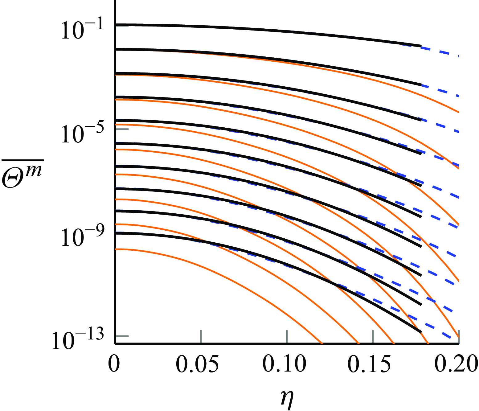
Constants $\gamma _{m}$
from (5.27) are shown for each moment up to order
$\gamma _{m}$
from (5.27) are shown for each moment up to order $n=10$
determined by fitting to the DNS, yielding the following fit:
$n=10$
determined by fitting to the DNS, yielding the following fit: $\gamma _m=-1.27m^{2} + 37.52m + 27.34$
.
$\gamma _m=-1.27m^{2} + 37.52m + 27.34$
.

To get a first hint towards the understanding of the emergence of (5.27) as a function of the radial coordinate $\eta$
, the MPSE (5.1) is transformed into cylindrical coordinates. Subsequently, the scaling laws (5.20)–(5.22) are introduced into the cylindrical-transformed MPSE, yielding
$\eta$
, the MPSE (5.1) is transformed into cylindrical coordinates. Subsequently, the scaling laws (5.20)–(5.22) are introduced into the cylindrical-transformed MPSE, yielding
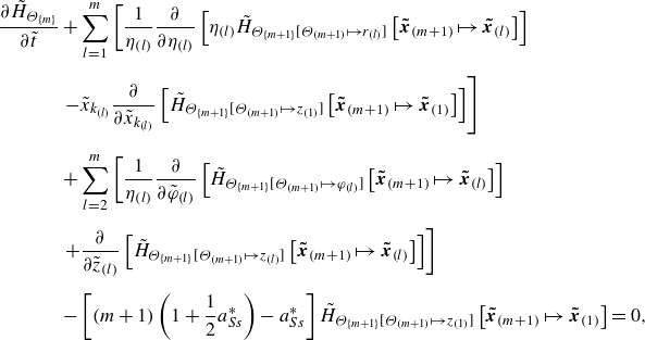 \begin{align} \frac {\partial \tilde {H}_{\Theta _{\{m\}}}}{\partial \tilde {t}}&+\sum _{l=1}^{m}\left [\frac {1}{\eta _{(l)}}\frac {\partial }{\partial \eta _{{(l)}}}\left [\eta _{(l)} \tilde {H}_{\Theta _{\{m+1\}}[\Theta _{(m+1)}\mapsto r_{(l)}]}\left [\boldsymbol{\tilde {x}}_{(m+1)}\mapsto \boldsymbol{\tilde {x}}_{(l)}\right ]\right ] \right . \nonumber \\[6pt] &\left . -\tilde {x}_{k_{(l)}}\frac {\partial }{\partial \tilde {x}_{k_{(l)}}}\left [\tilde {H}_{\Theta _{\{m+1\}}[\Theta _{(m+1)}\mapsto z_{(1)}]}\left [\boldsymbol{\tilde {x}}_{(m+1)}\mapsto \boldsymbol{\tilde {x}}_{(1)}\right ]\right ] \right ]\nonumber \\[6pt] &+\sum _{l=2}^{m}\left [\frac {1}{\eta _{(l)}}\frac {\partial }{\partial \tilde {\varphi }_{{(l)}}} \left [\tilde {H}_{\Theta _{\{m+1\}}[\Theta _{(m+1)}\mapsto \varphi _{(l)}]}\left [\boldsymbol{\tilde {x}}_{(m+1)}\mapsto \boldsymbol{\tilde {x}}_{(l)}\right ]\right ] \right . \nonumber \\[6pt] &\left .+\frac {\partial }{\partial \tilde {z}_{{(l)}}} \left [\tilde {H}_{\Theta _{\{m+1\}}[\Theta _{(m+1)}\mapsto z_{(l)}]}\left [\boldsymbol{\tilde {x}}_{(m+1)}\mapsto \boldsymbol{\tilde {x}}_{(l)}\right ]\right ] \right ]\nonumber \\[6pt] &-\left [(m+1)\left (1+\frac {1}{2}a_{Ss}^{*}\right )-a_{Ss}^{*}\right ]\tilde {H}_{\Theta _{\{m+1\}}[\Theta _{(m+1)}\mapsto z_{(1)}]}\left [\boldsymbol{\tilde {x}}_{(m+1)}\mapsto \boldsymbol{\tilde {x}}_{(1)}\right ]=0 ,\end{align}
for $m=1,\ldots , \infty$
and
$m=1,\ldots , \infty$
and $\tilde {x}_{k_{(l)}} \neq \tilde {\varphi }_{(l)}$
with a reference point
$\tilde {x}_{k_{(l)}} \neq \tilde {\varphi }_{(l)}$
with a reference point $\boldsymbol{\tilde {x}}_{(1)}$
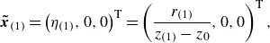 \begin{equation} \boldsymbol{\tilde {x}}_{(1)}=\left (\eta _{(1)},0,0\right )^\textrm{T} =\left (\frac {r_{(1)}}{z_{(1)}-z_0},0,0\right )^\textrm{T}, \end{equation}
and the points $\boldsymbol{\tilde {x}}_{(l)}$
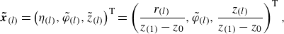 \begin{equation} \boldsymbol{\tilde {x}}_{(l)}=\left (\eta _{(l)}, \tilde {\varphi }_{(l)}, \tilde {z}_{(l)} \right )^\textrm{T}=\left (\frac {r_{(l)}}{z_{(1)}-z_0}, \tilde {\varphi }_{(l)}, \frac {z_{(l)}}{z_{(1)}-z_0}\right )^\textrm{T} ,\end{equation}
for $l=2,\ldots ,\infty$
and where
$l=2,\ldots ,\infty$
and where $\tilde {t}$
emerges from (5.12) as
$\tilde {t}$
emerges from (5.12) as
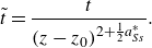 \begin{equation} \tilde {t}=\frac {t}{(z-z_0)^{2+\frac {1}{2}a_{Ss}^{*}}}. \end{equation}
Detailed steps for obtaining (5.29) and (5.32) can be taken from Appendix C. It is important to note that $\boldsymbol{\tilde {x}}_{(l)}$
must contain
$\boldsymbol{\tilde {x}}_{(l)}$
must contain $\tilde {\varphi }_{(l)}$
to ensure their unique definition. Equation (5.29) has been reduced by one independent variable through the scaling laws. After a symmetry reduction, the symmetry properties change in relation to the original equation. In particular, scaling symmetries can disappear, but various symmetries are also inherited. Presently, symmetries admitted by (5.29) include
$\tilde {\varphi }_{(l)}$
to ensure their unique definition. Equation (5.29) has been reduced by one independent variable through the scaling laws. After a symmetry reduction, the symmetry properties change in relation to the original equation. In particular, scaling symmetries can disappear, but various symmetries are also inherited. Presently, symmetries admitted by (5.29) include
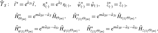 \begin{align} \tilde {\overline {T}}_{S}: \quad &\tilde {t}^{*}=\mathrm{e}^{\tilde {a}_{St}}\tilde {t}, \quad \eta _{(\cdot )} ^{*}=\mathrm{e}^{\tilde {a}_{S}}\eta _{(\cdot )}, \quad \tilde {\varphi }_{(\cdot )}^{*}=\tilde {\varphi }_{(\cdot )}, \quad \tilde {z}_{(\cdot )}^{*}=\tilde {z}_{(\cdot )}, \nonumber \\[6pt] &\tilde {H}_{\Theta _{\{m\}}}^{*}=\mathrm{e}^{m\tilde {a}_{S\theta }-\tilde {a}_{S}} \tilde {H}_{\Theta _{\{m\}}}, \quad \tilde {H}_{r_{\{1\}}\Theta _{\{m\}}}^{*}=\mathrm{e}^{m\tilde {a}_{S\theta }-\tilde {a}_{St}} \tilde {H}_{r_{\{1\}}\Theta _{\{m\}}}, \nonumber \\[6pt] &\tilde {H}_{\varphi _{\{1\}}\Theta _{\{m\}}}^{*}=\mathrm{e}^{m\tilde {a}_{S\theta }-\tilde {a}_{St}} \tilde {H}_{\varphi _{\{1\}}\Theta _{\{m\}}}, \quad \tilde {H}_{z_{\{1\}}\Theta _{\{m\}}}^{*}=\mathrm{e}^{m\tilde {a}_{S\theta }-\tilde {a}_{S}-\tilde {a}_{St}} \tilde {H}_{z_{\{1\}}\Theta _{\{m\}}}, \end{align}
with $\tilde {H}_{\Theta _{\{m+1\}}[\Theta _{(m+1)}\mapsto i_{(l)}]}=\tilde {H}_{i_{\{1\}}\Theta _{\{m\}}}$
and
$\tilde {H}_{\Theta _{\{m+1\}}[\Theta _{(m+1)}\mapsto i_{(l)}]}=\tilde {H}_{i_{\{1\}}\Theta _{\{m\}}}$
and $i_{(l)}=r_{(l)}, \varphi _{(l)}, z_{(l)}$
. However, caution is necessary regarding the scaling symmetries given here, because although inserting (5.33) into (5.29) seems to prove the symmetry properties, the symmetries (5.33) are not necessarily symmetries of the complete system (5.4) in reduced form. Therefore, we are dealing with a kind of partial invariance, which is not to be confused with the mathematical concept of partially invariant solutions (see e.g. Meleshko Reference Meleshko2005). The statistical symmetry (
$i_{(l)}=r_{(l)}, \varphi _{(l)}, z_{(l)}$
. However, caution is necessary regarding the scaling symmetries given here, because although inserting (5.33) into (5.29) seems to prove the symmetry properties, the symmetries (5.33) are not necessarily symmetries of the complete system (5.4) in reduced form. Therefore, we are dealing with a kind of partial invariance, which is not to be confused with the mathematical concept of partially invariant solutions (see e.g. Meleshko Reference Meleshko2005). The statistical symmetry ( $\tilde {a}_{Ss}$
) is inherited from (5.13)
$\tilde {a}_{Ss}$
) is inherited from (5.13)
 \begin{equation} \tilde {\overline {T}}_{Ss}: \boldsymbol{\tilde {x}}_{(\cdot )} ^{*}=\boldsymbol{\tilde {x}}_{(\cdot )}, \tilde {H}_{\Theta _{\{m\}}}^{*}=\mathrm{e}^{\tilde {a}_{Ss}} \tilde {H}_{\Theta _{\{m\}}}, \tilde {H}_{i_{\{1\}}\Theta _{\{m\}}}^{*}= \mathrm{e}^{\tilde {a}_{Ss}} \tilde {H}_{i_{\{1\}}\Theta _{\{m\}}}, \end{equation}
and the superposition symmetry of linear systems is presently given by
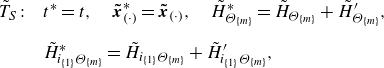 \begin{align} \tilde {T}_{S}:\quad & t^{*}=t, \quad \boldsymbol{\tilde {x}}_{(\cdot )} ^{*}=\boldsymbol{\tilde {x}}_{(\cdot )}, \quad \tilde {H}_{\Theta _{\{m\}}}^{*}=\tilde {H}_{\Theta _{\{m\}}}+\tilde {H}^{\prime}_{\Theta _{\{m\}}},\nonumber \\[6pt] & \tilde {H}_{i_{\{1\}}\Theta _{\{m\}}}^{*}= \tilde {H}_{i_{\{1\}}\Theta _{\{m\}}}+\tilde {H}^{\prime}_{i_{\{1\}}\Theta _{\{m\}}}, \end{align}
where the prime quantities are any additional independent solution of (5.29). Here, the superposition symmetry (5.35) plays a crucial role, as will be explained later. With the symmetries (5.33)–(5.34), a characteristic condition is, once again, derived
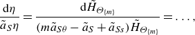 \begin{equation} \frac {\mathrm{d}\eta }{\tilde {a}_{S} \eta }=\frac {\mathrm{d}\tilde {H}_{\Theta _{\{m\}}}}{(m\tilde {a}_{S\theta } -\tilde {a}_{S}+\tilde {a}_{Ss})\tilde {H}_{\Theta _{\{m\}}}}=\ldots , \end{equation}
where non-relevant terms have been omitted. Integrating the characteristic condition (5.36) leads to
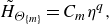 \begin{equation} \tilde {H}_{\Theta _{\{m\}}}=C_{m}\eta ^q, \end{equation}
where $C_{m}$
is the integration constant and
$C_{m}$
is the integration constant and
 \begin{equation} q=m\frac {\tilde {a}_{S\theta }}{\tilde {a}_{S}}+\frac {\tilde {a}_{Ss}}{\tilde {a}_{S}}-1. \end{equation}
For the connection of (5.27) to (5.37), the superposition symmetry (5.35) reveals its importance, allowing for a superposition of (5.37). The Taylor series of (5.27)
 \begin{equation} \mathrm{e}^{-\gamma _m \eta ^{2}}=1-\gamma _m\eta ^{2}+\frac {1}{2}\left (\gamma _m\eta ^{2}\right )^{2}-\frac {1}{6}\left (\gamma _m\eta ^{2}\right )^3+\ldots , \end{equation}
shows that (5.37) are the basis functions of (5.27). Therefore, the sum of the basis functions (5.37) can be written as
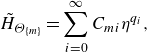 \begin{equation} \tilde {H}_{\Theta _{\{m\}}}=\sum _{i=0}^{\infty } C_{mi}\eta ^{q_i}, \end{equation}
where
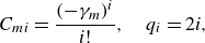 \begin{equation} C_{mi}=\frac {(-\gamma _m)^i}{i!}, \quad q_i=2i, \end{equation}
showing the importance of the intermittency symmetry and the superposition symmetry, which are both only admitted by the equations in the $H$
-formulation and not by the Euler or NSEs.
$H$
-formulation and not by the Euler or NSEs.
5.5. Gaussian behaviour of the higher mixed moments
We have gathered data for higher mixed moments up to $n+m=6$
, aiming to demonstrate their composition as a combination of axial velocity and passive scalar moments, similar to § 5.3.
$n+m=6$
, aiming to demonstrate their composition as a combination of axial velocity and passive scalar moments, similar to § 5.3.
The radial profiles (blue, dashed) of $m=1$
(top) up to the
$m=1$
(top) up to the $n+m=6$
(bottom) axial mixed moment
$n+m=6$
(bottom) axial mixed moment $\overline {U_z^n\Theta ^m}$
and the corresponding Gaussian (black) from (5.27) shown in a semi-logarithmic plot at
$\overline {U_z^n\Theta ^m}$
and the corresponding Gaussian (black) from (5.27) shown in a semi-logarithmic plot at $z/D=45$
.
$z/D=45$
.
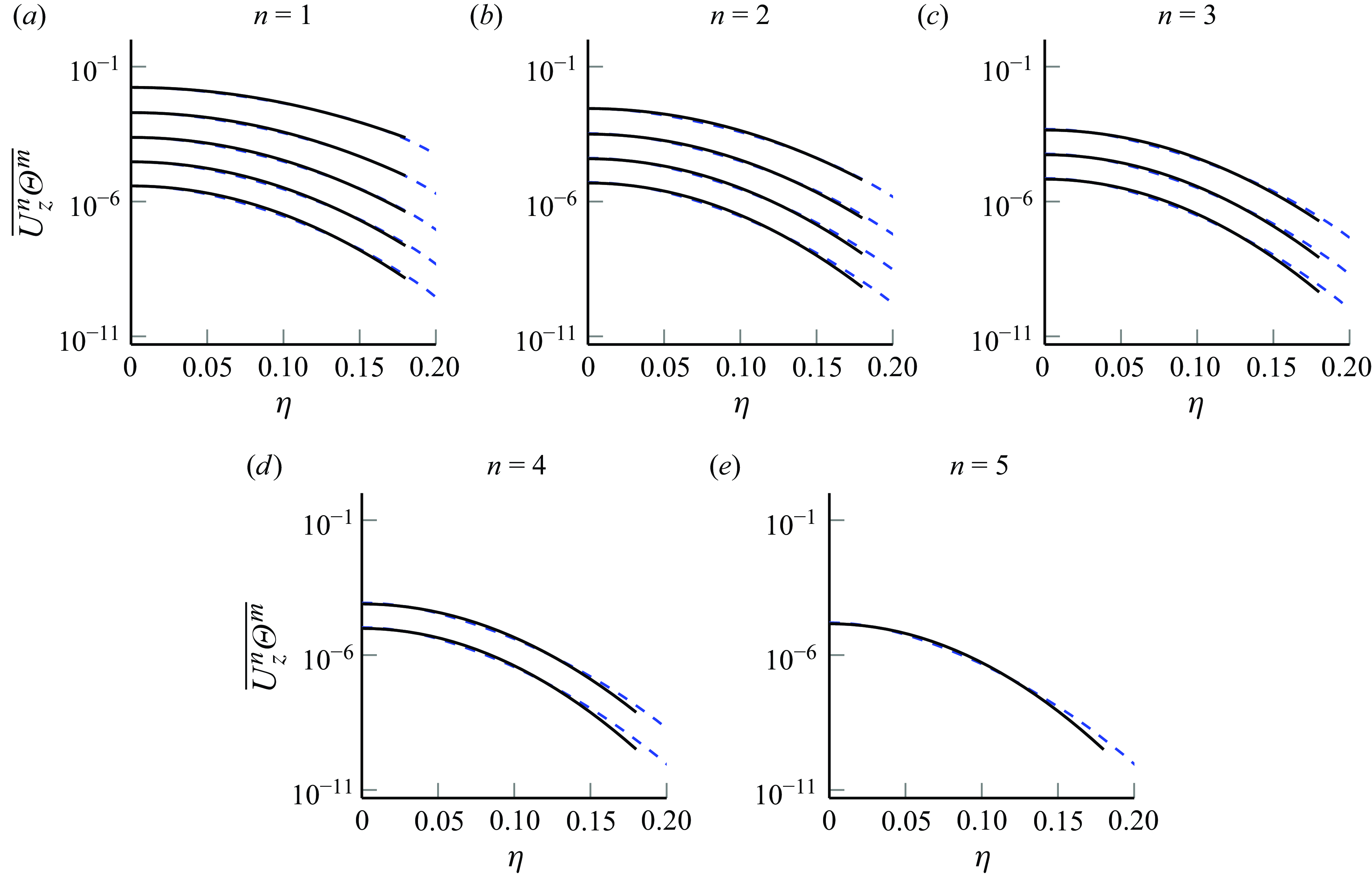
As illustrated in figure 18, we observe that the mixed moments also exhibit Gaussian behaviour at high precision. This characteristic is attributed to both the higher axial velocity and passive scalar moments displaying similar trends. In our recent study (Nguyen & Oberlack Reference Nguyen and Oberlack2024b ) for the axial velocity moments, we established
 \begin{equation} \frac {\overline {U_z^n}}{\overline {U_{z,c}^n}}=\widetilde {\overline {U_z^n}}(\eta )=\mathrm{e}^{-\gamma _n \eta ^{2}}, \end{equation}
where the Gaussian coefficient $\gamma _n$
was approximated by
$\gamma _n$
was approximated by
 \begin{equation} \gamma _n=-1.54n^{2}+61.95n+27.10. \end{equation}
From (5.27) and (5.42) we may invoke
 \begin{equation} \widetilde {\overline {U_z^n \Theta ^m}}(\eta )=\mathrm{e}^{-\gamma _{nm}\eta ^{2}}. \end{equation}
The subsequent approximation is a nonlinear $n$
-
$n$
- $m$
surface fit to the DNS data, as shown in figure 18, and is
$m$
surface fit to the DNS data, as shown in figure 18, and is
 \begin{equation} \gamma _{nm}=-1.51n^{2}-1.29m^{2}-0.03nm+61.2n+37.34m+30.75, \end{equation}
presented in figure 19 with a coefficient of determination of $R^{2}=0.99$
. The Gaussian coefficients
$R^{2}=0.99$
. The Gaussian coefficients $\gamma _n$
and
$\gamma _n$
and $\gamma _m$
in (5.43) and (5.28) respectively may be compared with
$\gamma _m$
in (5.43) and (5.28) respectively may be compared with $\gamma _{nm}$
in (5.45) by tentatively assuming
$\gamma _{nm}$
in (5.45) by tentatively assuming $\widetilde {\overline {U_z^n}}\,\widetilde {\overline {\Theta ^m}}\approx \widetilde {\overline {U_z^n \Theta ^m}}$
, which implies
$\widetilde {\overline {U_z^n}}\,\widetilde {\overline {\Theta ^m}}\approx \widetilde {\overline {U_z^n \Theta ^m}}$
, which implies $\gamma _{n}+\gamma _{m}\approx \gamma _{nm}$
. Comparing the Gaussian coefficients of (5.28), (5.43) and (5.45) reveals an approximate halving of the constant terms and the emergence of a small cross-product term, while the remaining terms only differ by
$\gamma _{n}+\gamma _{m}\approx \gamma _{nm}$
. Comparing the Gaussian coefficients of (5.28), (5.43) and (5.45) reveals an approximate halving of the constant terms and the emergence of a small cross-product term, while the remaining terms only differ by $2\, \%$
. This observation suggests that the moments are coupled and demonstrate some degree of cross-correlation. Nevertheless, the approximation (5.45) reduces approximately to the special forms (5.28) and (5.43) in the limit cases
$2\, \%$
. This observation suggests that the moments are coupled and demonstrate some degree of cross-correlation. Nevertheless, the approximation (5.45) reduces approximately to the special forms (5.28) and (5.43) in the limit cases $n=0$
and
$n=0$
and $m=0$
.
$m=0$
.
Constants $\gamma _{nm}$
from (5.44) are shown for pure moments up to order
$\gamma _{nm}$
from (5.44) are shown for pure moments up to order $n,m=10$
and mixed moments up to order
$n,m=10$
and mixed moments up to order $n+m=6$
determined by fitting to the DNS yielding the following fit:
$n+m=6$
determined by fitting to the DNS yielding the following fit: $\gamma _{nm}=-1.51n^{2}-1.29m^{2}-0.03nm+61.2n+37.34m+30.75$
.
$\gamma _{nm}=-1.51n^{2}-1.29m^{2}-0.03nm+61.2n+37.34m+30.75$
.
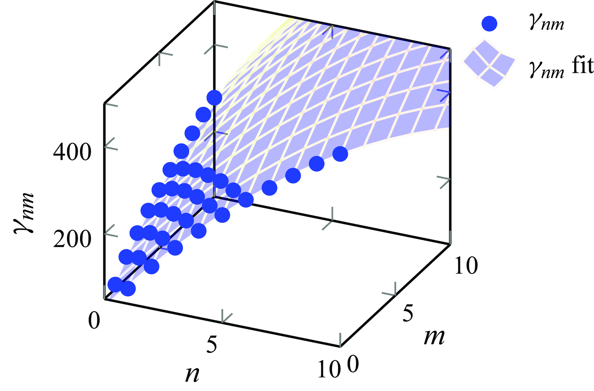
6. Conclusion
This study has two integral components: a comprehensive DNS investigation of a turbulent round jet flow including a scalar and the derivation of group invariant solutions using Lie-symmetry analysis applied to the MPVSCEs, validated by the DNS.
The DNS effort yielded new and detailed data on the passive scalar concentration up to the tenth-order moments for a turbulent round jet at $Re=3500$
and
$Re=3500$
and $Pr=0.71$
. Additionally, previously unreported mixed velocity–passive scalar moments up to the sixth order were extracted. The highly converged data, averaged over
$Pr=0.71$
. Additionally, previously unreported mixed velocity–passive scalar moments up to the sixth order were extracted. The highly converged data, averaged over $75\,000 D/U_b$
time units, exhibited a remarkable collapse in radial profiles for various statistics in
$75\,000 D/U_b$
time units, exhibited a remarkable collapse in radial profiles for various statistics in $z/D=10$
intervals in the range
$z/D=10$
intervals in the range $z/D=15{-}55$
.
$z/D=15{-}55$
.
Lie-symmetry analysis has been applied to a system of differential equations consisting of the MPSE and the multi-point velocity–passive scalar equations, a combination of the MPSE and MPMEs. Both have been derived in their $H$
-form (instantaneous form) from which, using their symmetries, a set of self-similar solutions, also called turbulent scaling laws, have been derived. The resulting scaling laws are then validated against the aforementioned DNS, demonstrating a remarkable agreement up to the tenth order and for mixed moments up to the sixth order, linking the scaling laws for the velocity and passive scalar moments. The group parameter of the statistical scaling symmetry, allowing a possible variation of the turbulent decay behaviour in turbulent round jets, is uniquely defined by the inflow condition.
$H$
-form (instantaneous form) from which, using their symmetries, a set of self-similar solutions, also called turbulent scaling laws, have been derived. The resulting scaling laws are then validated against the aforementioned DNS, demonstrating a remarkable agreement up to the tenth order and for mixed moments up to the sixth order, linking the scaling laws for the velocity and passive scalar moments. The group parameter of the statistical scaling symmetry, allowing a possible variation of the turbulent decay behaviour in turbulent round jets, is uniquely defined by the inflow condition.
An intriguing observation emerged from the study of the pure instantaneous passive scalar moments, revealing a Gaussian-like behaviour found in the radial direction only in statistical symmetries, similar to the pure axial velocity moments. The higher moments were accurately represented by Gaussian functions linked by a nonlinear coefficient $\gamma _m$
, challenging the assumption of linear behaviour due to the dominance of the mean. This nonlinear behaviour, exemplified by the parameter
$\gamma _m$
, challenging the assumption of linear behaviour due to the dominance of the mean. This nonlinear behaviour, exemplified by the parameter $\gamma _m$
and in the Gaussian function, signifies intermittency, reinforcing the findings in the PDF and higher standardised moments. Furthermore, the Gaussian behaviour extends to mixed axial velocity–scalar moments, where the coefficient
$\gamma _m$
and in the Gaussian function, signifies intermittency, reinforcing the findings in the PDF and higher standardised moments. Furthermore, the Gaussian behaviour extends to mixed axial velocity–scalar moments, where the coefficient $\gamma _{nm}$
indicates that the axial velocity and the scalar exhibit a clear correlation.
$\gamma _{nm}$
indicates that the axial velocity and the scalar exhibit a clear correlation.
Acknowledgements
The authors gratefully acknowledge the Gauss Centre for Supercomputing e.V. (www.gauss-centre.eu) for funding this project under the project number pn73fu by providing computing time on the GCS Supercomputer SUPERMUC-NG at Leibniz Supercomputing Centre (www.lrz.de).
Funding
C.T.N. wants to acknowledge the funding from the Studienstiftung des deutschen Volkes (Academic Scholarship Foundation) and M.O. gratefully acknowledges partial funding by the Deutsche Forschungsgemeinschaft (DFG, German Research Foundation) - SPP 2410 Hyperbolic Balance Laws in Fluid Mechanics: Complexity, Scales, Randomness (CoScaRa), within the Project ‘Approximation Methods for Statistical Conservation Laws of Hyperbolically Dominated Flow’ under project number 526024901.
Declaration of interests
The authors report no conflict of interest.
Data availability statement
The data that support the findings of this study are openly available in the TUdatalib Repository of the Technical University of Darmstadt at https://doi.org/10.48328/tudatalib-1756.
Appendix A. Derivation of the multi-point scalar equations
This appendix shows the derivation of the MPSE. The starting point is the passive scalar equation at one point $\boldsymbol{x} \in \mathbb{R}^{3}$
 \begin{equation}{\mathcal{S}}(\boldsymbol{x}) =\frac {\partial \Theta (\boldsymbol{x},t)}{\partial t} + U_{k}(\boldsymbol{x},t) \frac {\partial \Theta (\boldsymbol{x},t)}{\partial x_{k}} -\frac {1}{Pe} \frac {\partial ^{2}\Theta (\boldsymbol{x},t)} {\partial {x_{k}} \partial {x_{k}}}=0. \end{equation}
The two-point passive scalar equation can then be received through statistically averaging the cross-multiplication of (A1) and the passive scalar at different points $\boldsymbol{x}$
and
$\boldsymbol{x}$
and $\boldsymbol{y}\in {\mathbb{R}^{3}}$
 \begin{equation} \mathcal{S}_2=\overline {\mathcal{S}(\boldsymbol{x})\Theta (\boldsymbol{y})+\mathcal{S}(\boldsymbol{y})\Theta (\boldsymbol{x})}=0 ,\end{equation}
leading to
 \begin{eqnarray} {\mathcal{S}_2} &=&\frac {\partial H_{\Theta \Theta }(\boldsymbol{x},\boldsymbol{y})}{\partial t}+\frac {\partial H_{\Theta \Theta k}(\boldsymbol{x},\boldsymbol{y},\boldsymbol{x})}{\partial x_k}+\frac {\partial H_{\Theta \Theta k}(\boldsymbol{y},\boldsymbol{x},\boldsymbol{y})}{\partial y_k}\nonumber \\[6pt]&&-\, \frac {1}{Pe} \left (\frac {\partial ^2 H_{\Theta \Theta }(\boldsymbol{x},\boldsymbol{y})}{\partial x_k\partial x_k}+ \frac {\partial ^2 H_{\Theta \Theta }(\boldsymbol{x},\boldsymbol{y})}{\partial y_k\partial y_k}\right )=0, \end{eqnarray}
where $H_{\Theta \Theta }(\boldsymbol{x},\boldsymbol{y})=\overline {\Theta (\boldsymbol{x})\Theta (\boldsymbol{y})}$
and
$H_{\Theta \Theta }(\boldsymbol{x},\boldsymbol{y})=\overline {\Theta (\boldsymbol{x})\Theta (\boldsymbol{y})}$
and $H_{\Theta \Theta k}(\boldsymbol{x},\boldsymbol{y},\boldsymbol{x})=\overline {\Theta (\boldsymbol{x})\Theta (\boldsymbol{y})U_k(\boldsymbol{x})}$
. This can be extended up to an arbitrary order
$H_{\Theta \Theta k}(\boldsymbol{x},\boldsymbol{y},\boldsymbol{x})=\overline {\Theta (\boldsymbol{x})\Theta (\boldsymbol{y})U_k(\boldsymbol{x})}$
. This can be extended up to an arbitrary order $m$
by introducing the MPSE
$m$
by introducing the MPSE
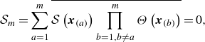 \begin{equation} {\mathcal{S}_m}=\sum _{a=1}^{m} \overline {{\mathcal{S}}\left (\boldsymbol{x}_{(a)}\right ) \prod _{b=1,b\neq a}^{m} \Theta \left (\boldsymbol{x}_{(b)}\right )}=0 ,\end{equation}
where $\Theta (\boldsymbol{x}_{(i)} )$
is a passive scalar at different points
$\Theta (\boldsymbol{x}_{(i)} )$
is a passive scalar at different points $\boldsymbol{x}_{(i)}\in \mathbb{R}^{3}$
. Plugging (A1) into (A4) then yields
$\boldsymbol{x}_{(i)}\in \mathbb{R}^{3}$
. Plugging (A1) into (A4) then yields
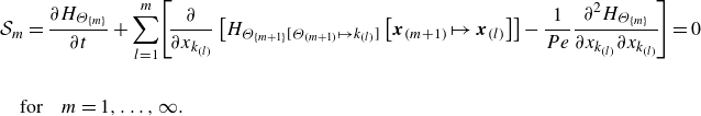 \begin{align} &{\mathcal{S}_m} =\frac {\partial H_{\Theta _{\{m\}}}}{\partial t}+\sum _{l=1}^{m} \! \left [\! \frac {\partial }{\partial x_{k_{(l)}}} \left [H_{\Theta _{\{m+1\}}[\Theta _{(m+1)}\mapsto k_{(l)}]}\left [\boldsymbol{x}_{(m+1)}\mapsto \boldsymbol{x}_{(l)}\right ] \right ] -\frac {1}{Pe}\frac {\partial ^{2} H_{\Theta _{\{m\}}}}{\partial x_{k_{(l)}}\partial x_{k_{(l)}}} \! \right ]=0 \nonumber\\[16pt]&\quad \textrm{for} \quad m=1,\ldots ,\infty . \end{align}
Appendix B. Derivation of the multi-point velocity–scalar equations
In this appendix, the derivation of the MPVSCEs is shown. With (A1) and the moment (2.2)
 \begin{equation} {\mathcal{M}_i}(\boldsymbol{x})=\frac {\partial U_i(\boldsymbol{x},t)}{\partial t}+U_k(\boldsymbol{x},t) \frac {\partial U_i(\boldsymbol{x},t)}{\partial x_{k}}+\frac {\partial P(\boldsymbol{x},t)}{\partial x_i}-\frac {1}{Re} \frac {\partial ^{2}U_i(\boldsymbol{x},t)}{\partial x_{k}\partial x_{k}}=0, \end{equation}
the two-point velocityscalar correlation equations can be derived with
 \begin{equation} {\mathcal{T}_{i\Theta }}=\overline {\mathcal{M}_i(\boldsymbol{x})\Theta (\boldsymbol{y})+U_i(\boldsymbol{x}){\mathcal{S}}(\boldsymbol{y})}, \end{equation}
which, by inserting (A1) and (B1), can be extended to
 \begin{eqnarray} {\mathcal{T}}_{i\Theta } &=& \frac {\partial H_{i\Theta }(\boldsymbol{x},\boldsymbol{y})}{\partial t}+\frac {\partial H_{i\Theta k}(\boldsymbol{x},\boldsymbol{y},\boldsymbol{x})}{\partial x_{k}}+\frac {\partial H_{\Theta i k}(\boldsymbol{y},\boldsymbol{x},\boldsymbol{y})}{\partial y_{k}} \nonumber \\[16pt] && + \, \frac {\partial \overline {P(\boldsymbol{x})\Theta (\boldsymbol{y})}}{\partial x_i}- \left (\frac {1}{Re}\frac {\partial ^{2} H_{i\Theta }(\boldsymbol{x},\boldsymbol{y})}{\partial x_{k}\partial x_{k}}+ \frac {1}{Pe} \frac {\partial ^{2} H_{i\Theta }(\boldsymbol{x},\boldsymbol{y})}{\partial y_{k}\partial y_{k}}\right )=0. \end{eqnarray}
Similarly to (A4), two-point velocity–scalar correlation equations can be extended to the MPVSCEs for $n$
velocities at
$n$
velocities at $n$
different points and
$n$
different points and $m$
passive scalars at
$m$
passive scalars at $m$
different points
$m$
different points
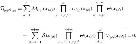 \begin{eqnarray} {\mathcal{T}}_{i_{\{n\}}\Theta _{\{m\}}} &=&\sum _{a=1}^{n} \overline {\mathcal{M}_{i_{(a)}}(\boldsymbol{x}_{(a)})\prod _{c=1,c\neq a}^{n} U_{i_{(c)}}(\boldsymbol{x}_{(c)})\prod _{d=n+1}^{n+m} \Theta (\boldsymbol{x}_{(d)})} \nonumber \\[16pt] && +\, \sum _{a=n+1}^{n+m} \overline {{\mathcal{S}}(\boldsymbol{x}_{(a)})\prod _{c=n+1,c\neq d}^{n+m} \Theta (\boldsymbol{x}_{(c)})\prod _{d=1}^{n} U_{i_{(d)}}(\boldsymbol{x}_{(d)})}=0. \end{eqnarray}
By introducing (B1) and (A1) into (B4), we receive the MPVSCEs
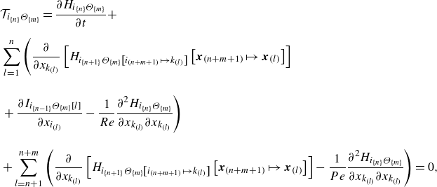 \begin{align} &{\mathcal{T}}_{i_{\{n\}}\Theta _{\{m\}}}=\frac {\partial H_{i_{\{n\}}\Theta _{\{m\}}}}{\partial t}+\nonumber \\[6pt] & \sum _{l=1}^{n} \left (\frac {\partial }{\partial x_{k_{(l)}}}\left [H_{i_{\{n+1\}}\Theta _{\{m\}}\left [i_{(n+m+1)}\mapsto k_{(l)}\right ]}\left [\boldsymbol{x}_{(n+m+1)}\mapsto \boldsymbol{x}_{(l)} \right ]\right ] \right. \nonumber\\[12pt] &\left. +\, \frac {\partial I_{i_{\{n-1\}}\Theta _{\{m\}}\left [ l\right ]}}{\partial x_{i_{(l)}}} -\frac {1}{Re}\frac {\partial ^{2} H_{i_{\{n\}}\Theta _{\{m\}}}}{\partial x_{k_{(l)}} \partial x_{k_{(l)}}}\right )\nonumber \\[10pt] & +\sum _{l=n+1}^{n+m} \left (\frac {\partial }{\partial x_{k_{(l)}}}\left [H_{i_{\{n+1\}}\Theta _{\{m\}}\left [i_{(n+m+1)}\mapsto k_{(l)}\right ]}\left [\boldsymbol{x}_{(n+m+1)}\mapsto \boldsymbol{x}_{(l)} \right ]\right ]-\frac {1}{Pe}\frac {\partial ^{2} H_{i_{\{n\}}\Theta _{\{m\}}}}{\partial x_{k_{(l)}} \partial x_{k_{(l)}}}\right )=0, \nonumber\\\end{align}
The MPVSCEs (B5) are therefore a generalisation of the MPMEs and the MPSEs. The MPMEs can be obtained for $m=0$
, while the MPSEs arise for
$m=0$
, while the MPSEs arise for $n=0$
.
$n=0$
.
Appendix C. Reduction of the multi-point scalar equation
This appendix shows a step-by-step derivation of the reduced MPSE in cylindrical coordinate form. For this, the MPSE (5.1) is transformed to cylindrical coordinates while considering $Re^{-1}, Pe^{-1} =0$
has been employed, yielding
$Re^{-1}, Pe^{-1} =0$
has been employed, yielding
 \begin{align} \frac {\partial H_{\Theta _{\{m\}}}}{\partial t}&+ \,\frac {1}{r_{(1)}}\frac { \partial }{\partial r_{(1)}} \left [r_{(1)} H_{\Theta _{\{m+1\}}[\Theta _{(m+1)}\mapsto r_{(1)}]}\left [\boldsymbol{x}_{(m+1)}\mapsto \boldsymbol{x}_{(1)}\right ]\right ] \nonumber \\[6pt] &+\,\frac {\partial }{\partial z_{(1)}} \left [H_{\Theta _{\{m+1\}}[\Theta _{(m+1)}\mapsto z_{(1)}]}\left [\boldsymbol{x}_{(m+1)}\mapsto \boldsymbol{x}_{(1)}\right ]\right ] \nonumber \\[6pt] &+\,\sum _{l=2}^{m}\left [\frac {1}{r_{(l)}}\frac {\partial }{\partial r_{(l)}} \left [r_{(l)} H_{\Theta _{\{m+1\}}[\Theta _{(m+1)}\mapsto r_{(l)}]}\left [\boldsymbol{x}_{(m+1)}\mapsto \boldsymbol{x}_{(l)}\right ]\right ] \right . \nonumber \\[6pt] & \left . +\,\frac {1}{r_{(l)}}\frac {\partial }{\partial \varphi _{(l)}} \left [H_{\Theta _{\{m+1\}}[\Theta _{(m+1)}\mapsto \varphi _{(l)}]}\left [\boldsymbol{x}_{(m+1)}\mapsto \boldsymbol{x}_{(l)}\right ]\right ] \right . \nonumber \\[6pt] & \left . +\,\frac {\partial }{\partial z_{(l)}} \left [H_{\Theta _{\{m+1\}}[\Theta _{(m+1)}\mapsto z_{(l)}]}\left [\boldsymbol{x}_{(m+1)}\mapsto \boldsymbol{x}_{(l)}\right ]\right ] \right ]=0, \end{align}
where the reference point is
 \begin{equation} \boldsymbol{x}_{(1)}=\left (r_{(1)}, 0, z_{(1)}\right )^\textrm{T} ,\end{equation}
and
 \begin{equation} \boldsymbol{x}_{(l)}=\left ( r_{(l)}, \varphi _{{(l)}}, z_{(l)} \right )^\textrm{T}, \end{equation}
for $l=2,\ldots ,\infty$
. For the sake of completeness, the scaling of the time
$l=2,\ldots ,\infty$
. For the sake of completeness, the scaling of the time $t$
shall be considered. Using the symmetry (5.12), the characteristic condition (5.14) extends to
$t$
shall be considered. Using the symmetry (5.12), the characteristic condition (5.14) extends to
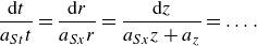 \begin{equation} \frac {\mathrm{d}t}{a_{St}t}=\frac {\mathrm{d}r}{a_{Sx}r}=\frac {\mathrm{d}z}{a_{Sx}z+a{_{z}}}=\ldots . \end{equation}
By considering the symmetry breaking (5.19) and integrating the first and third terms of (C4), the scaling law of the time $t$
yields
$t$
yields
 \begin{equation} \tilde {t}=\frac {t}{(z-z_0)^{2+\frac {1}{2}a_{Ss}^{*}}}. \end{equation}
In the next step, $\boldsymbol{x}$
is reduced by one independent variable by considering the scaling law (5.20), leading to the reference point
$\boldsymbol{x}$
is reduced by one independent variable by considering the scaling law (5.20), leading to the reference point
 \begin{equation} {\tilde{\boldsymbol{x}}}_{(1)}=(\eta_{(1)},0,0 )^{\textrm{T}} =\left (\frac{r_{(1)}}{z_{(1)} - z_{0}},0,0 \right)^{\textrm{T}}, \end{equation}
and the points ${\tilde{\boldsymbol{x}}}_{(l)}$
 \begin{equation} {\tilde{\boldsymbol{x}}}_{(l)}=\left (\eta _{(l)}, \tilde {\varphi }_{(l)}, \tilde {z}_{(l)} \right )^{\textrm{T}}=\left (\frac {r_{(l)}}{z_{(1)}-z_0}, \tilde {\varphi }_{(l)}, \frac {z_{(l)}}{z_{(1)}-z_0}\right )^{\textrm{T}}, \end{equation}
for $l=2,\ldots ,\infty$
. Finally, the scaling laws (C5) and (5.20)–(5.22) derived through Lie-symmetry analysis are deployed into (C1), yielding the reduced MPSE
$l=2,\ldots ,\infty$
. Finally, the scaling laws (C5) and (5.20)–(5.22) derived through Lie-symmetry analysis are deployed into (C1), yielding the reduced MPSE
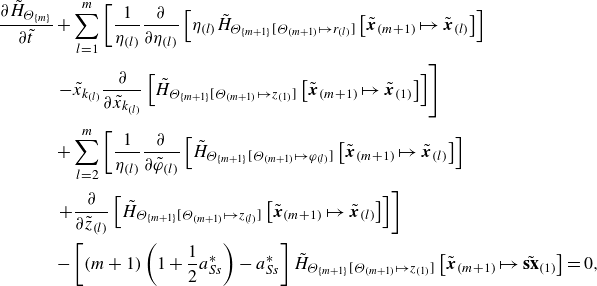 \begin{align} \frac {\partial \tilde {H}_{\Theta _{\{m\}}}}{\partial \tilde {t}}&+\sum _{l=1}^{m}\left [\frac {1}{\eta _{(l)}}\frac {\partial }{\partial \eta _{{(l)}}}\left [\eta _{(l)} \tilde {H}_{\Theta _{\{m+1\}}[\Theta _{(m+1)}\mapsto r_{(l)}]}\left [{\tilde{\boldsymbol{x}}}_{(m+1)}\mapsto {\tilde{\boldsymbol{x}}}_{(l)}\right ]\right ] \right . \nonumber \\[2pt] &\left . -\tilde {x}_{k_{(l)}}\frac {\partial }{\partial \tilde {x}_{k_{(l)}}}\left [\tilde {H}_{\Theta _{\{m+1\}}[\Theta _{(m+1)}\mapsto z_{(1)}]}\left [{\tilde{\boldsymbol{x}}}_{(m+1)}\mapsto {\tilde{\boldsymbol{x}}}_{(1)}\right ]\right ] \right ]\nonumber \\[2pt] &+\sum _{l=2}^{m}\left [\frac {1}{\eta _{(l)}}\frac {\partial }{\partial \tilde {\varphi }_{{(l)}}} \left [\tilde {H}_{\Theta _{\{m+1\}}[\Theta _{(m+1)}\mapsto \varphi _{(l)}]}\left [{\tilde{\boldsymbol{x}}}_{(m+1)}\mapsto {\tilde{\boldsymbol{x}}}_{(l)}\right ]\right ] \right . \nonumber \\[2pt] &\left .+\frac {\partial }{\partial \tilde {z}_{{(l)}}} \left [\tilde {H}_{\Theta _{\{m+1\}}[\Theta _{(m+1)}\mapsto z_{(l)}]}\left [{\tilde{\boldsymbol{x}}}_{(m+1)}\mapsto {\tilde{\boldsymbol{x}}}_{(l)}\right ]\right ] \right ]\nonumber \\[2pt] &-\left [(m+1)\left (1+\frac {1}{2}a_{Ss}^{*}\right )-a_{Ss}^{*}\right ]\tilde {H}_{\Theta _{\{m+1\}}[\Theta _{(m+1)}\mapsto z_{(1)}]}\left [{\tilde{\boldsymbol{x}}}_{(m+1)}\mapsto {\tilde{\textbf{sx}}}_{(1)}\right ]=0 , \nonumber\\\end{align}
and $\tilde {x}_{k_{(l)}} \neq \tilde {\varphi }_{(l)}$
.
$\tilde {x}_{k_{(l)}} \neq \tilde {\varphi }_{(l)}$
.


 Open access