


I. Introduction and overview
This research examines the factors affecting the adoption of barrel-aging by US craft brewers from 2008 to 2014, with a special focus on peer effects from being in proximity to nearby breweries. The growth of craft brewing in the US has coincided with an explosion of new or reintroduced beer styles and processes outside of the typical lager or brown ale. Resurgent styles such as India Pale Ales (IPA) are closely identified with the craft beer movement, but barrel-aged (BA) beers have also become increasingly popular. Tracing its origins to Belgian brewing, aging in wooden barrels is not a wholly modern technique. For most 21st-century brewers and consumers, however, it is a fairly novel trend. Like many wines, a BA beer is aged anywhere from weeks to years to impart woody flavors into the beer before it is packaged and sold. Because this process is less efficient and often involves costlier ingredients, BA beers tend to be priced higher than other craft beers and released with limited production amounts and distribution.
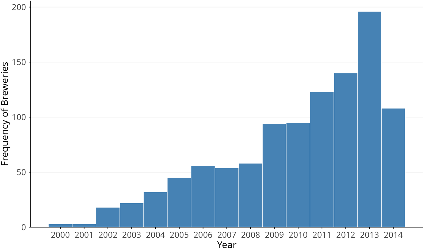
Using data gathered from RateBeer in a process described in Section 4.1, Figure 1 plots the distribution of an estimate of the number of US breweries in each year that released a BA beer for the first time. Some volume in the later years is driven by the large count of breweries founded during those years, not just existing breweries deciding to introduce a BA beer.
Distribution of years that craft breweries introduced a barrel-aged beer for the first time.

Figures 2 and 3 display county-level counts of the number of breweries in the data that had ever released a BA beer by 2008 and 2014, respectively. The 2008 map displays an initial concentration of barrel-aging among pre-existing concentrations of craft brewers: San Diego, the San Francisco Bay area, the Pacific Northwest, the Front Range of Colorado, Austin, the Upper Midwest, and lower New England. By 2014, those areas continued to intensify in counts, including the distinction of Chicago from the surrounding area, and the emergence of some areas such as Asheville, North Carolina and Portland, Maine.Footnote 1
Geographic distribution of breweries with barrel-aged beer by 2008. Cumulative count at county level. (Total: 291 breweries).

Geographic distribution of breweries with barrel-aged beer by 2014. Cumulative count at county level. (Total: 1047 breweries).

Since many craft breweries operate on a small scale and concentrate their sales locally, it is an open question as to how a trend like this diffuses throughout the country. Does the trend spread through brewer interaction on this local scale, where breweries adopt trends through mimicry or “me-too” competitive behavior? Or are brewers more likely to introduce a BA beer if they are located in cities where craft beer itself is much more popular, such that areas without many breweries are less likely to adopt? Or is there no real local pattern at all, so that breweries are more likely to adopt the trend as it grows on a nationwide level? Aspects of all three scenarios are likely at work.
I employ probit techniques to model the probability that a brewery releases a BA beer for the first time in a given year. I take care to avoid the common pitfalls of peer-effects analysis by addressing reflexivity by lagging and controlling for unobserved effects through a Mundlak–Chamberlain (MC) device. Combining review data from RateBeer with production data from the Brewers Association, I analyze the decisions of over 3,000 breweries that had not yet released a BA beer by the beginning of the period of study. Using several different definitions of “neighboring brewery” that vary based on the distance to the brewery in question (5, 10, 20, 50, and 100 miles), I find that the number of neighboring breweries who have released a BA beer by a particular year is positively associated with the probability the brewery will release one for the first time in the next year. This result remains after controlling for both the size of the neighboring brewing industry in general and nationwide trends, both in the total number of barrel-aging breweries and the number of craft brewers. However, when comparing the marginal effect of a neighboring brewery on the likelihood of barrel-aging to the marginal effect of the nationwide increase in barrel-aging, the aggregate nationwide trend has a substantially larger cumulative effect on the likelihood that a brewery begins to barrel-age.
These results suggest that nearby peers have a nonzero but limited influence on the brewing techniques of a craft brewery. The results themselves cannot distinguish between the effect of brewers finding inspiration from observing peers (mimicry) and the effect of learning about BA techniques from peers (knowledge spillovers). However, considering that barrel-aging involves more skill and knowledge of equipment than many other styles and because the craft industry is usually marked by a collaborative spirit over a hyper-competitive one, spillovers from geographical proximity cannot be easily ruled out. Nonetheless, the much stronger influence of the national BA trend suggests that while geography still matters in idea diffusion, access to information over other conduits like the Internet and national trade organizations plays a prominent role, at least as far as the diffusion of new beer styles is concerned.
The paper is organized as follows: Section 2 outlines the literature on craft brewer decision-making and the importance of local collaboration within the industry, along with a general overview of the geographic peer effects literature. Section 3 outlines the random-effects probit model along with the MC device. Section 4 describes the data sources and collection methods. Section 5 reports and discusses the empirical results, and Section 6 concludes.
II. Literature review
a. Craft brewing and industry concentration
Spatial relationships between craft brewers likely matter for the introduction of new products due to the drivers of local geographic concentration in the industry. The craft brewing industry in the US is notably hyperlocalized, with regional concentration of breweries emerging across the country. This clustering fosters collaboration and support among microbrewers who often share information and resources to promote industry growth at the local level (Alonso, Reference Alonso2011; Fouad and Scott, Reference Fouad and Scott2024). Such collaboration is facilitated by spatial proximity, enabling knowledge sharing, especially concerning tacit manufacturing practices (Nilsson et al., Reference Nilsson, Reid and Lehnert2018). Larger craft brewers frequently support smaller ones through shared resources and technical assistance, highlighting the hyper-localized nature of the industry (Nilsson et al., Reference Nilsson, Reid and Lehnert2018). Additionally, the home-brewing movement has been instrumental in the industry's growth, serving as an incubator for future commercial brewers (Murray and O'Neill, Reference Murray and O'Neill2012).
The decision over whether to introduce a new variation, such as barrel-aging, often plays an important role in a craft brewer's competitive strategy. Craft breweries aim to distinguish themselves from mass-produced beers by focusing on small-scale production of unique, high-quality beers often using local ingredients and traditional methods (Swaminathan, Reference Swaminathan1998; Swann, Reference Swann2012; Watne and Hakala, Reference Watne and Hakala2013; Wells, Reference Wells2016). This differentiation caters to consumers who value quality and variety over standardized products (Toro-González et al., Reference Toro-González, McCluskey and Mittelhammer2014).
Geographic, economic, and cultural factors significantly influence the decisions of craft brewers regarding market entry and beer styles. Local regulations, religious beliefs, and state-level economic conditions play crucial roles in the presence of breweries in different regions (Baginski and Bell, Reference Baginski and Bell2011; Gohmann, Reference Gohmann2016). The concentration of craft breweries in specific neighborhoods (Nilsson et al., Reference Nilsson, Reid and Lehnert2018) further suggests that geographic proximity influences the adoption of similar styles and trends within an area. The geographic distribution of craft breweries indicates a pattern of spatial contagion, where the success of breweries in one area inspires entrepreneurial activity in other regions (Swaminathan, Reference Swaminathan1998).
Beyond craft brewing, the economics literature has much to say about the advantages and challenges of industry clusters. Firms cluster to benefit from agglomeration economies such as lower transportation costs, improved information flows, shared labor pools, knowledge spillovers, and access to a variety of inputs (Artz et al., Reference Artz, Kim and Orazem2016; Baptista and Swann, Reference Baptista and Swann1998). However, congestion and competition effects can limit cluster growth (Baptista and Swann, Reference Baptista and Swann1998). Empirical research on clustering shows mixed results regarding innovation and entrepreneurship, with some studies highlighting the positive impact of clusters on these aspects (Delgado et al., Reference Delgado, Porter and Stern2010), while others find limited support for intentional, policy-driven cluster-promotion (Duranton, Reference Duranton2011). Analyses of particular industry clusters such as semiconductor and tire manufacturing in Silicon Valley and Ohio, respectively, note that employees leaving an established firm to start their own nearby spin-off is an important channel through which knowledge diffuses locally (Buenstorf and Klepper, Reference Buenstorf and Klepper2010; Klepper Reference Klepper2010).
The size of a firm influences its location choice and the benefits it receives from agglomeration. As Marshall (Reference Marshall1920) posited over a century ago, larger firms have an advantage in innovation due to economies of scale in research and development. Larger firms tend to be more geographically concentrated and benefit from knowledge spillovers, while smaller firms often form in clusters to benefit from the spillovers generated by larger firms (Holmes and Stevens, Reference Holmes and Stevens2002; Lafourcade and Mion, Reference Lafourcade and Mion2007). Glaeser et al. (Reference Glaeser, Kerr and Ponzetto2010) note that the entrepreneurial nature of smaller new entrants lends itself to faster growth than larger firms, and a larger local supply of entrepreneurial people supports this type of entry.
b. Peer effects
Several pieces of applied work highlight how proximity to similar firms or the density of them in a given area significantly impacts the adoption of new practices and technologies. Studies such as Graziano and Gillingham (Reference Graziano and Gillingham2015) on residential solar photovoltaic systems, and Conley and Udry (Reference Conley and Udry2010) on pineapple cultivation in Ghana, for example, demonstrate that technology adoption is positively driven by the density of nearby adopters.
Studies such as Lewis et al. (Reference Lewis, Barham and Robinson2011) and Correa (Reference Correa2023) on organic dairy farming provide a good template for how to isolate peer effects from general geographic location patterns. Theoretically, neighboring farmers help mitigate the uncertainty associated with the conversion to organic techniques by reducing the fixed costs of learning. Through analyzing the timing and location of adoption patterns, these studies find that the density of nearby organic farms positively influences adoption likelihood. This effect intensifies when neighboring farms share similar characteristics, underscoring the significance of “cognitive” proximity alongside geographical proximity. In addition to finding similar results, Marton and Storm (Reference Marton and Storm2021) also uncover a negative impact on organic conversion when nearby farms revert to conventional methods.
To avoid spurious correlations, shared environmental factors and individual characteristics must be accounted for to avoid overestimating or underestimating true peer effects (Graziano and Gillingham, Reference Graziano and Gillingham2015; Lewis et al., Reference Lewis, Barham and Robinson2011). This includes addressing homophily, where individuals with similar preferences or characteristics tend to locate together, potentially misinterpreted as peer effects. Reflexivity can bias estimates of peer effects if neighboring activity is correlated with the activity of the individual because the individual is, in part, influencing the peers, not just the other way around. Defining and measuring proximity accurately is also important. Proximity can refer to geographical distance, social distance within networks, or cognitive distance based on shared knowledge or industry. In the context of craft brewing, there is undoubtedly some spillover through networks not based on geography (such as membership organizations or online communities), but the underlying assumption made here is that geographic proximity through neighborhood effects plays a detectable role.
Finally, the peer effect variable may correlate with the error term in the model (endogeneity), which can occur due to simultaneity or omitted variable bias, leading to biased and inconsistent estimates. Various econometric techniques can mitigate endogeneity concerns, such as using instrumental variables (IVs; Klier and McMillen, Reference Klier and McMillen2008) or employing panel data to control for time-invariant unobserved heterogeneity (Lewis et al., Reference Lewis, Barham and Robinson2011). These approaches help isolate peer effects from other confounding factors by focusing on within-individual or within-group changes over time. As Lewis et al. (Reference Lewis, Barham and Robinson2011) point out, though, IV estimation is more suitable when the peer effect comes from the propensity to have nearby influences, while the hypothesis here is that the actual existence of neighbors is the source of influence. As explained in Section 3.1, I address these issues using an MC device in the estimation.
III. Empirical model
a. Random effects probit
Following the literature, especially on the spatial diffusion of organic farming techniques (Correa, Reference Correa2023; Lewis et al., Reference Lewis, Barham and Robinson2011; Marton and Storm, Reference Marton and Storm2021), I first consider a random-effects probit model estimated by Gaussian quadrature where the dependent variable for a brewery in year t is equal to 0 if a brewery has not yet released a BA beer in or by year t and equal to 1 if the brewery releases its very first BA beer in year t. For years after the year of first BA introduction (i.e., years after the t in which Ynt = 1), the brewery is dropped from the data. The random effect is unique to each brewery and constant over the entire time frame in which the brewery appears in the data. The panel of data is unbalanced since breweries may enter or exit within the period of study, and once a brewery releases a BA beer, they are dropped out of the data in the following years.
With Φ()˙ denoting the standard normal cumulative distribution function, the probability that brewery n releases a BA beer in year t (i.e., the probability that Ynt = 1) is conditional on several regressors as represented in the equation below:
 \begin{align}
{\text{P}}_{\text{r}}\left( Y_{nt}\, = \,1\left| {w_n},{x_{nt},{nba}_{nt - 1},z_{t},\mu n} \right. \right)\, &= \,\Phi \left( {w_n}\alpha + {X'}_{nt}\beta \, + {nba'}_{nt-1} \delta \, + {Z'}_{t}\eta \, \right.\cr
&\left. \quad + {\mu _n}\, + { \in _{nt}} \right).
\end{align}
\begin{align}
{\text{P}}_{\text{r}}\left( Y_{nt}\, = \,1\left| {w_n},{x_{nt},{nba}_{nt - 1},z_{t},\mu n} \right. \right)\, &= \,\Phi \left( {w_n}\alpha + {X'}_{nt}\beta \, + {nba'}_{nt-1} \delta \, + {Z'}_{t}\eta \, \right.\cr
&\left. \quad + {\mu _n}\, + { \in _{nt}} \right).
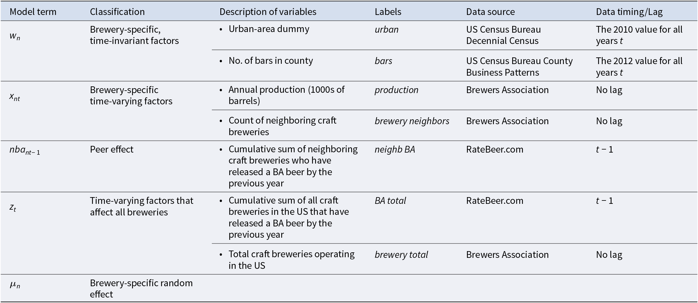
\end{align}Table 1 provides an explanation of the terms along with the data sources used in the empirical estimation. A further explanation of these data sources is provided in Section 4.
Description of Variables Potentially Included in the Model

If unobserved effects that influence the decision to adopt are also correlated with the regressors, the estimate of the peer effect, nba, could be biased. For example, breweries within a particular neighborhood might experience some common shock that affects supply-side factors like simultaneous exposure to barrel-aging techniques through something other than proximity. Alternatively, unobserved demand for BA styles could create a spatial dependence between breweries, reflective in part or whole of a common response to demand.
I account for these unobservables in the estimation in a few ways. First, a count of all breweries nationwide that have released a BA beer before time t is included as a regressor. This is meant to control for the potential for breweries to be influenced by the overall trend in barrel-aging. Second, a count of all existing breweries in time t as a regressor controls for time trends emanating from the overall growth of breweries in the US. Third, nba is a count lagged by 1 year, minimizing issues with reflexivity. Fourth, in a robustness check in Section 5.2, I estimate a model with a control for the number of barsFootnote 2 in the brewery’s county (variable bars in Table 1). As explained further in Section 4.3, this is a way to test the sensitivity of the model to the inclusion of a control that can indicate something about local demand for craft beer or style variety.
As far as other explicit controls in the model are concerned: urban controls for potential effects that urbanization has on making adoption easier, production controls for any effects that brewery size has on adoption, and brewery neighbors controls for the effect that a density of neighboring brewers, independent of whether they barrel age, has on adoption.
Finally, unobserved brewery-specific factors fixed across time can be addressed using an MC device (Chamberlain, Reference Chamberlain1982; Mundlak, Reference Mundlak1978) that essentially estimates the random effect µn as a function of a mean-zero normally-distributed random variable, ωn ∼ N(0,σ), and the averages of the brewery-specific time-varying variables.Footnote 3 In this case, these are the peer effect (nba), production, and brewery neighbors. The parameters ϕ, χ, and ψ are to be estimated in the equation for µn below:
 \begin{equation}{\mu _n} = {\omega _n} + \overline {neighb\_B{A_n}}\phi + \overline{productio{n_n}}\chi + \overline{brewery\_neighbor{s_n}}\psi \end{equation}
The MC device serves as a control for time-invariant unobserved effects that affect an individual brewery. For example, if particular regions around the brewery have a higher disposition to demand BA beers that is linked to unobserved but unchanging factors, the MC device controls for these. One would have to argue that remaining bias in nba comes from unobserved demand or homophily factors that are both time-varying over the sample period and idiosyncratic to the brewery’s region.
To the extent the estimate of σ, the standard deviation of the random effect is estimated to be insignificantly different from zero, and the model can be estimated following Papke and Wooldridge (Reference Papke and Wooldridge2008), Cameron and Trivedi (Reference Cameron and Trivedi2005), and Cameron et al. (Reference Cameron, Gelbach and Miller2008). This alternative method estimates the model as a pooled probit where cluster-robust standard errors are bootstrapped using 500 replications of the brewery cross-sections. As with Lewis et al. (Reference Lewis, Barham and Robinson2011) and Correa (Reference Correa2023), this approach should be robust to heteroskedasticity and serial correlation for each brewery. Indeed, initial estimates of my random-effects model using either unadjusted errors or errors clustered by brewery found that σ is insignificantly different from zero.Footnote 4 Thus, I proceed with the pooled model with bootstrapped errors as the main estimation method, where the main equation to be estimated is:
 \begin{align}
\Pr\left( {{Y_{nt\,}}\, = \,1|\,{w_n},{x_{nt}},nb{a_{nt - 1}},Zt,{\mu _n}} \right)\, &= \,{\alpha _1}urba{n_{n\,}}\, + \,{\beta _1}productio{n_{nt}}\, \cr
&\quad + \!{\beta _2}brewery\_neighbor{s_{nt}}\! + \!{\delta _1}neighb\_B{A_{nt - 1}}\, \cr
&\quad + \!\eta _1^{}BA\_tota{l_{t - 1}}\, + \,{\eta _2}brewery\_tota{l_{t\,}}\, + \,{\omega _{n}} \cr
&\quad + \!{\phi _1} \overline{neighb\_{BA_n}}\, + \,{X_1}\overline{productio{n_n}}\cr
&\quad + \!{\psi _1}\overline{brewery\_neighbor{s_n}} + \,{ \in _{nt}}
\end{align}
\begin{align}
\Pr\left( {{Y_{nt\,}}\, = \,1|\,{w_n},{x_{nt}},nb{a_{nt - 1}},Zt,{\mu _n}} \right)\, &= \,{\alpha _1}urba{n_{n\,}}\, + \,{\beta _1}productio{n_{nt}}\, \cr
&\quad + \!{\beta _2}brewery\_neighbor{s_{nt}}\! + \!{\delta _1}neighb\_B{A_{nt - 1}}\, \cr
&\quad + \!\eta _1^{}BA\_tota{l_{t - 1}}\, + \,{\eta _2}brewery\_tota{l_{t\,}}\, + \,{\omega _{n}} \cr
&\quad + \!{\phi _1} \overline{neighb\_{BA_n}}\, + \,{X_1}\overline{productio{n_n}}\cr
&\quad + \!{\psi _1}\overline{brewery\_neighbor{s_n}} + \,{ \in _{nt}}
\end{align}b. Neighboring distance
I use a distance-based definition of who a brewery's neighboring peer breweries are, where a brewery is included as a peer if they are within “X” miles of the primary location of the brewery in question, as determined by Euclidean (straight-line) distance. For any given specification, I estimate five separate models varying X from 5, 10, 20, 50, and 100 miles.Footnote 5
IV. Data
a. RateBeer
The data on when BA beers are first introduced comes from the ratings website RateBeer.com. The website hosted millions of ratings of hundreds of thousands of beers from tens of thousands of breweries worldwide, so it contained an incredibly wide and deep coverage of brewing activity. Through a data-scraping process I employed in 2015, from this database, a list of beers was selected that are tagged with phrases such as “barrel-aged,” “bourbon barrel,” “wine barrel,” and others that are meant to be used to identify beers that have been aged in wooden barrels at some point during production. The beers were then grouped by brewery, and within a grouping of a brewery's ratings, the very first year a brewery's BA beer appeared with a rating was considered to be the year in which the brewery began barrel-aging. Although there is some lag time between a beer's commercial introduction and its initial entry on RateBeer, the website is popular enough that the year of first review should serve as a good proxy. From this beer list, approximately 1,339 breweries in the US were identified as having produced a BA beer between 2000 and part of 2015.
Unfortunately, no further data acquisition from RateBeer in this manner can occur due to website and policy changes made since 2015, and as of February 1, 2025, RateBeer has permanently shut down.Footnote 6
b. Brewers Association
Yearly taxable production data by brewery is available from the Brewers Association, the key trade association for the craft brewing industry in the US. According to their tally, the US had 3,464 commercial craft brewers as of 2014 (1,871 microbreweries, 1,412 brewpubs, and 135 regional breweries). These data are available starting from 2008. These data are especially important for determining when a brewer enters or exits. If a brewery appears in the production data for the first time in year t, then I assume that t is when they enter. If they stop appearing after year t, then I assume they have exited by year t + 1, and they are dropped from the data in those remaining years.Footnote 7 Entry and exit data also inform the calculation of brewery neighbors and brewery total. The measure brewery neighbors captures the number of breweries within some X distance of the brewery in question and is intended to proxy for the size of the local craft brewing industry agglomeration and the potential for standard agglomeration externalities. The measure brewery total, a count of all operating craft breweries in a particular year, can capture any effects from national growth in the industry over time, and its monotonic growth may also capture some more general time trends.
Combining RateBeer and Brewers Association data provides 8,749 brewery-year observations.
c. Census/Other government data
The urban/rural classification from the 2010 US Decennial Census is used to control for whether a brewery's location is in an urban area. This can highlight differences in knowledge diffusion through agglomeration economies that tend to be more prominent in urban areas.
As a rudimentary test of whether more explicitly controlling for demand characteristics affects the nba parameter, in one specification, I control for the number of bars in a brewery’s county. This operates under the assumption that areas with more bars tend to have a higher demand for craft beer and new styles, which may influence decisions independently of urban size or local industry spillovers. These data are sourced from the Census’s 2012 County Business Patterns. A single year is chosen in order to capture cross-sectional differences, where I assume that variation over time within a particular county is insignificant or not indicative of fluctuating underlying demand for new styles. For example, the period under study coincides with the 2007–2009 recession and subsequent recovery, where macroeconomic effects on both supply and demand likely influence temporary variation in establishments, not changes in consumer preferences.
V. Empirical results
a. Baseline model
The baseline model includes the regressors neighb BA (t – 1) (nbant − 1), production, brewery neighbors, urban, BA total, brewery total, and the cross-sectional average variables for the MC device. Since MC variables merely address issues with correlated unobserved effects, I do not attempt to interpret the coefficient estimates concerning their impact on the dependent variable.
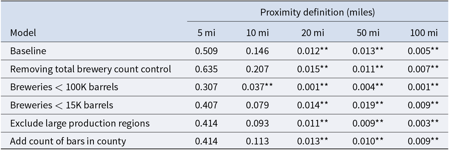
While the baseline model leverages a methodological approach following the previously referenced spatial diffusion studies (Correa, Reference Correa2023; Lewis et al., Reference Lewis, Barham and Robinson2011; Marton and Storm, Reference Marton and Storm2021), permutation-based Moran's I tests (reported in Appendix A) reveal that residual spatial autocorrelation is present in several model specifications, especially with broader geographic neighbor definitions (20 miles and above). A standard approach to correcting spatially correlated errors in nonlinear panel models would be clustering at a higher level, but doing so at the county level does not fix this issue. This suggests the spatial dependence of residuals operates across county boundaries and is not fully captured by clustering at the county level. The next level of geographic hierarchy, the state level, is likely too broad. To my knowledge, more complex models that account for this spatial dependence in errors have not been validated for use with the methodology used in diffusion studies of this scope involving nonlinear methods and large unbalanced panels.
Consequently, results for specifications and distance bands where spatial autocorrela-tion persists should be interpreted with this caveat: statistical significance of the affected regressions may be overstated. Notably, spatial autocorrelation is mostly absent in the 5- and 10-mile distance-band models, and, as shown below, the substantive conclusions from these models closely track those for larger radius definitions: peer effects are found to be relatively minor compared to the strong influence of the nationwide barrel-aging trend.
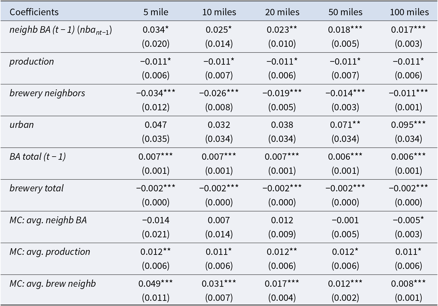
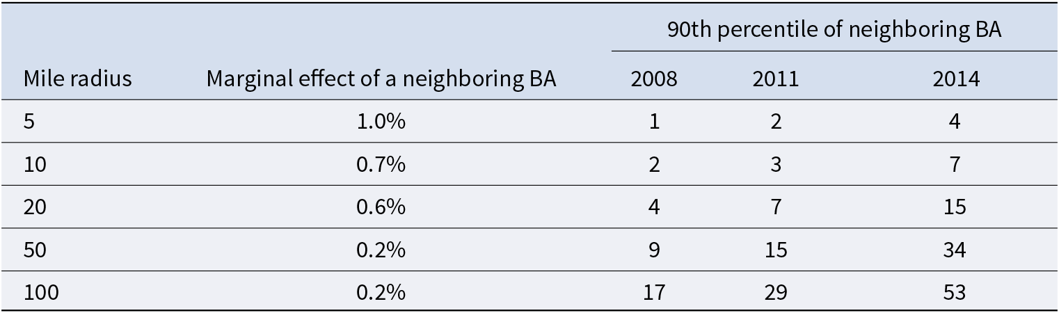
The results of the baseline model with the five different distance-based definitions of neighboring breweries are displayed in Table 2. The coefficients on the peer effect neighb BA (t − 1) are statistically significant at the 10% level or less for all radius definitions. However, shorter radii (5 and 10 miles) are not significant at the 5% level. Converting the probit parameter effects to marginal effects in Table 3 suggests that the per-brewery influence of barrel-aging is declining as the radius increases, which is expected. However, overall, the influence of each marginal brewery on the likelihood that a brewery begins barrel-aging is not especially large across the typical brewer's peers. For example, the largest marginal impact is under the 5-mile definition, where each additional brewery that has begun barrel-aging is associated with an increase in the likelihood that a brewery begins barrel-aging by 1 percentage point. Considering that the interquartile range of neighb BA (t − 1) under the 5-mile radius is only 1 by 2014, this marginal effect of 1 percentage point also represents the typical cumulative impact of peer influence within 5 miles. By 2014, only 10% of breweries had 53 or more barrel-aging peers within 100 miles, indicating a cumulative impact of 10.6% or more on the likelihood for this 10% subset of breweries.
Coefficient Estimates on Baseline Model

Standard errors in parentheses.
Signif. Codes: ***:0.01, **: 0.05, *: 0.1.
Marginal Effect of neighb BA (t − 1) (Count of Neighboring BA Breweries)

The importance of national trends is highlighted by the influence of the statistically significant BA total coefficient (the count of all BA breweries nationwide in the previous year). Given the coefficients for BA total across the different proximity definition columns, the marginal effect of an additional BA brewery anywhere in the US is an increase in the likelihood of another brewery releasing a BA beer for the first time of 0.07–0.2 percentage points. In 2007, 208 active breweries had released a BA beer by that year. In 2013, this number was 871. Cumulatively, this means that this nationwide trend had an additive effect of 14.56–41.6 percentage points on the likelihood of beginning to barrel age in 2008 and 60.97–174.2 percentage points in 2014. Naturally, the total likelihood cannot surpass 100 percent, so this latter range is before the addition of other independent variables that have a negative effect on the likelihood. Also, the likely existence of diminishing effects suggests that a simple linear extrapolation is a very crude approximation.
Interestingly, coefficients for the number of breweries in general are negative. The coefficient on brewery neighbors, which is a count of nearby craft breweries within a specified radius, is negative and diminishing in size as the radius increases. The coefficient on brewery total, a count of all US breweries in a given year, is negative and consistent in size across all radii. On the surface, this suggests that the size of the local brewing agglomeration has an inverse effect on the likelihood of barrel-aging, while the growing size of the craft brewing industry overall has a similar inverse effect. At a local level, the coefficient on brewery neighbors suggests that breweries in smaller agglomerations are more likely to release BA beers for the first time, but this could also reflect the idea that breweries in older, larger agglomerations were more likely to have released their BA beers by the time the period under study begins. I leave open the possibility that these variables, especially brewery total, are capturing other nationwide or local time trends affecting the general growth of craft brewing that are not accounted for in the model.
The coefficient on urban is not consistently statistically significant across radius definitions, but it is always positive. To the extent the true effect is positive and statistically different from zero, this suggests that urban-based breweries are more likely to introduce a BA beer. This could reflect the positive effect of urbanization on the introduction of new ideas and variety. The coefficient on production is negative and statistically significant, suggesting an inverse effect of brewery size on BA introduction. While this suggests that smaller breweries are more likely to develop and introduce a new product idea, the large (small) breweries that had not yet introduced a BA beer by 2008 might not be representative of all large (small) breweries, including the ones that introduced a BA beer pre-2008, which are not included as observations.
b. Robustness checks
i. Regression specifications and subsamples
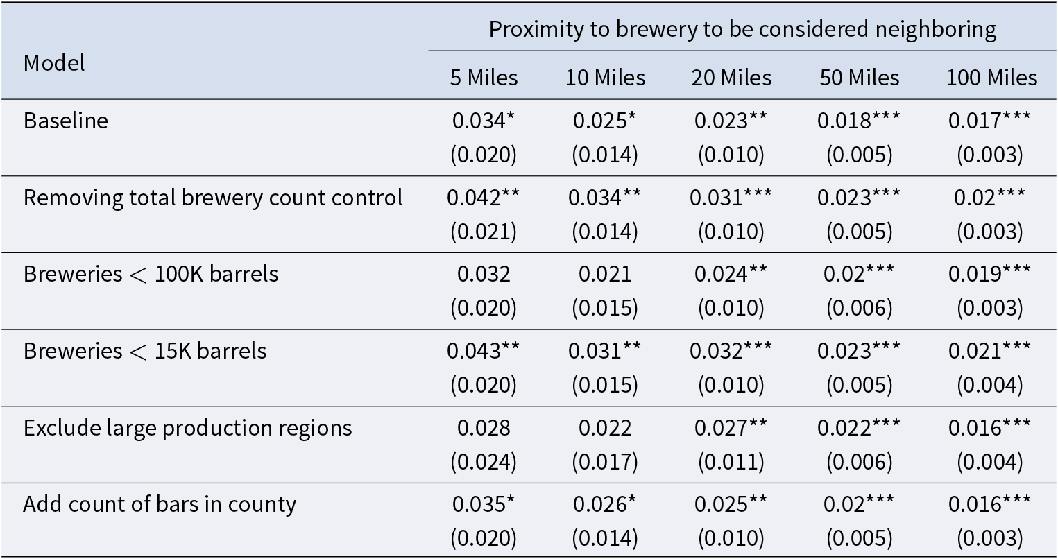
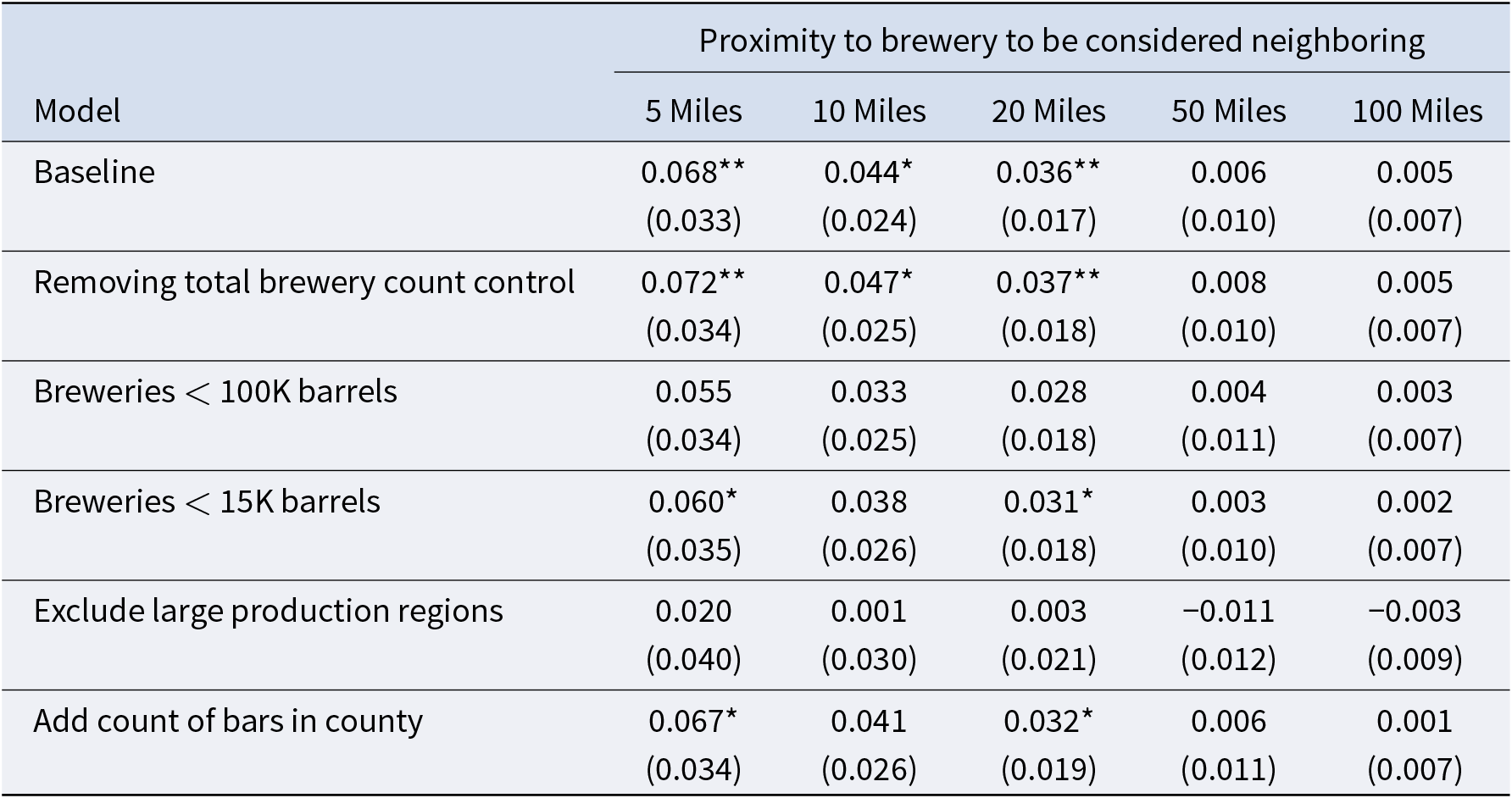
Table 4 reports estimates of the neighb BA (t – 1) term (the peer effect) across distance definitions and several differing models to test robustness. Besides the baseline model incorporating all breweries, I estimate a model without brewery total to demonstrate whether a control for overall craft brewery growth impacts the estimates. I estimate the baseline model on a subset of breweries that brew fewer than 100,000 barrels per year and a subset that brews fewer than 15,000 per year. “Microbrewery” is usually defined as an operation brewing less than 15,000 barrels, and these could be impacted differently than large breweries in terms of access to information and resources. I also estimate a model excluding Combined Statistical Areas (CSAs)Footnote 8 where the total barrels brewed among all breweries in that CSA was greater than 500,000 in 2014. This tests whether large outlier metro areasFootnote 9 and outlier breweries,Footnote 10 skew results. Finally, I estimate a model on the baseline sample that adds a control for the count of bars in the brewery’s county in 2012. This acts as a simple control for time-invariant underlying local demand that the MC device may not fully capture.
Coefficient Estimates of neighb BA (t − 1) Under Different Models or Samples

Standard-errors in parentheses.
Signif. Codes: ***: 0.01, **: 0.05, *: 0.1.
The coefficient estimates in Table 4 suggest that changing the model and samples in these ways do not substantially affect the estimate of nba. If anything, the largest difference seems to be for the microbrewery subsample, where the impacts of barrel-aging peers are slightly larger than the estimates for the full sample. In other words, peer effects might be more important for smaller-scale breweries. Overall, though, the size and significance of the baseline results do not appear to be driven by large breweries and large brewing regions in the sample. Furthermore, the fact that including a simple control for the count of local drinking establishments changes little about the coefficients on nba does not suggest that this peer effect, already estimated alongside the MC device, is driven by other omitted local demand characteristics.
ii. Twice-lagged regressors
As an additional check, I run all 30 regressions with the inclusion of twice-lagged (t − 2) regressors for neighb BA, BA total, and the brewery-averaged neighb BA for the MC device. Full results are available in Appendix B. Potential multicollinearity from incorporating two lags of the same variable might be driving those results overall, so caution is warranted when interpreting size and significance. Nonetheless, it is notable that for the neighb BA coefficients, the once-lagged (t − 1) estimates are still positive and significant for the baseline specification and several other robustness checks for the 5- and 10-mile bands, those least affected by spatial autocorrelation. At the very least, including twice-lagged regressors demonstrates that the effect of neighb BA still matters, but potentially the peer influence could come through from the state of the “neighbors” 2, not just 1, years previous.
iii. Separate distance bins
The model used in this paper accounts for neighboring barrel-aging breweries and neighboring breweries in total by estimating any given specification or subsample five times: one where a neighbor is defined as between 0 and 5 miles away, another where it is between 0 and 10 miles away, and so on up to 0 and 100 miles away.
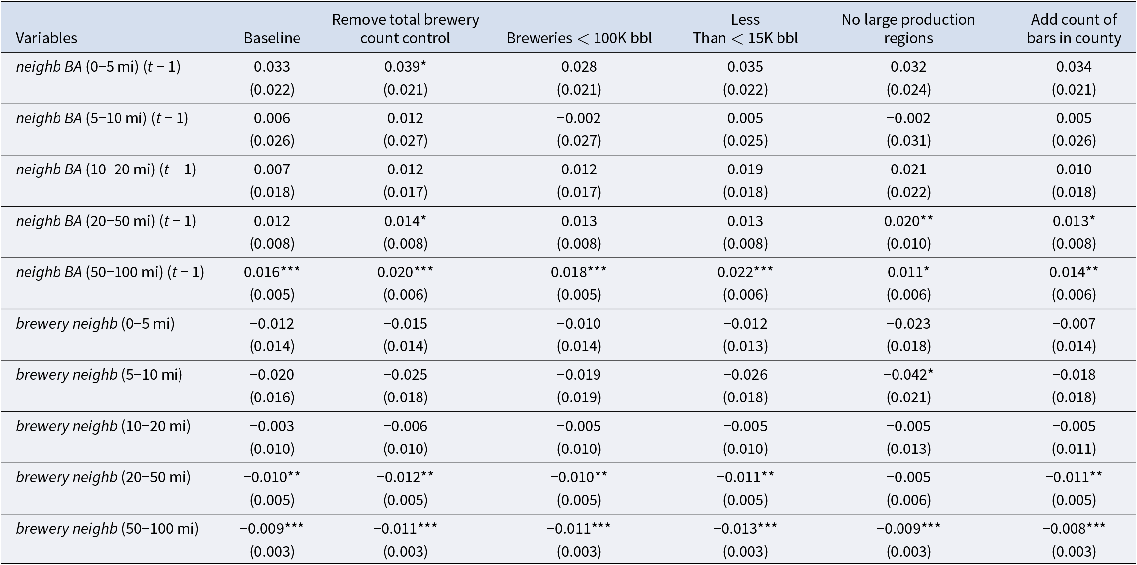
Following specifications used in other parts of the spatial proximity literature (see Graziano and Gillingham (Reference Graziano and Gillingham2015), Moore et al. (Reference Moore, Doubek, Xu and Cardinale2020), and Graziano et al. (Reference Graziano, Liu, Meyer and Zhang2024) as examples), I re-estimate the baseline model and all robustness checks with an alternative specification that uses five regressors in the same estimation that account for the number of barrel-aging neighbors from 0 to 5, >5 to ≤10, >10 to ≤20, >20 to ≤50, and > 50 to ≤100 miles away from the brewery in question. When controlling for the number of neighboring breweries in general (not just barrel-aging ones), an additional five regressors are included in the equation in a similar way. In other words, instead of regression equation (3), estimated with:
 \begin{equation*}\ldots + {\beta _2}brewery\_neighbors{\left( {{\text{0-X mi}}} \right)_{nt}} + {\delta _1}neighb\_BA{\left( {{\text{0-X mi}}} \right)_{nt}}_{ - 1} + \ldots\end{equation*}
where X is either 5, 10, 20, 50, or 100, an equation is estimated with:
 \begin{equation}\begin{gathered}
\ldots + {\beta _2}brewery\_neighbors{\left( {{\text{0-5 mi}}} \right)_{nt}} + {\beta _3}brewery\_neighbors{\left( {{\text{5-10 mi}}} \right)_{nt}} \hfill \\
+ {\beta _4}brewery\_neighbors{\left( {{\text{10-20 mi}}} \right)_{nt}} + {\beta _5}brewery\_neighbors{\left( {{\text{20-50 mi}}} \right)_{nt}} \hfill \\
+ {\beta _6}brewery\_neighbors{\left( {{\text{50-100 mi}}} \right)_{nt}} + {\delta _1}neighb\_BA{\left( {{\text{0-5 mi}}} \right)_{nt}}_{ - 1} \hfill \\
+ {\delta _2}neighb\_BA{\left( {{\text{5-10 mi}}} \right)_{nt}}_{ - 1} + {\delta _3}neighb\_BA{\left( {{\text{10-20 mi}}} \right)_{nt}}_{ - 1} \hfill \\
+ {\delta _4}neighb\_BA{\left( {{\text{20-50 mi}}} \right)_{nt}}_{ - 1} + {\delta _5}neighb\_BA{\left( {{\text{50-100 mi}}} \right)_{nt}}_{ - 1} + \ldots \hfill \\
\end{gathered} \end{equation}
\begin{equation}\begin{gathered}
\ldots + {\beta _2}brewery\_neighbors{\left( {{\text{0-5 mi}}} \right)_{nt}} + {\beta _3}brewery\_neighbors{\left( {{\text{5-10 mi}}} \right)_{nt}} \hfill \\
+ {\beta _4}brewery\_neighbors{\left( {{\text{10-20 mi}}} \right)_{nt}} + {\beta _5}brewery\_neighbors{\left( {{\text{20-50 mi}}} \right)_{nt}} \hfill \\
+ {\beta _6}brewery\_neighbors{\left( {{\text{50-100 mi}}} \right)_{nt}} + {\delta _1}neighb\_BA{\left( {{\text{0-5 mi}}} \right)_{nt}}_{ - 1} \hfill \\
+ {\delta _2}neighb\_BA{\left( {{\text{5-10 mi}}} \right)_{nt}}_{ - 1} + {\delta _3}neighb\_BA{\left( {{\text{10-20 mi}}} \right)_{nt}}_{ - 1} \hfill \\
+ {\delta _4}neighb\_BA{\left( {{\text{20-50 mi}}} \right)_{nt}}_{ - 1} + {\delta _5}neighb\_BA{\left( {{\text{50-100 mi}}} \right)_{nt}}_{ - 1} + \ldots \hfill \\
\end{gathered} \end{equation}Coefficients β 2 through β 6 and δ 1 through δ 5 capture the marginal impact of a neighbor being within that particular band of distance. The MC device also includes the cross-sectional averages of the five distance bins for the barrel-aging breweries and breweries in general.
Full results for this specification are available in Table C1 in Appendix C. For the measures of neighboring breweries that have barrel aged, typically only the count of breweries within 50–100 miles (“neighb BA (50–100 mi) (t − 1)”) is statistically significant. This could be explained by possible multicollinearity: since breweries tend to cluster within metro regions, a brewery with a relatively large number of close neighbors is also likely to have a relatively large number of neighbors further away. Like the results in Table 4, where only the larger distance measures (20, 50, and 100 miles) are consistently statistically significant, if insignificance in Table C1 is due to multicollinearity, this provides further evidence that there is little difference in influence between breweries within the same general region that are very close versus further away. Additionally, ignoring influence from breweries further out may understate peer effects. Looking again at Table C1, the coefficient estimates for neighb BA (50–100 mi) (t − 1) are of similar size to the “100 Miles” column of Table 4. The coefficient estimate of 0.016 for neighb BA (50–100 mi) (t − 1) in the Baseline model translates to a marginal effect of about 0.2% on the likelihood of barrel-aging. This effect is the same size as one for an additional brewery within 0–100 miles, as indicated on the last row of Table 3.
VI. Conclusion
This research seeks to determine the relative importance of local peer influence versus national trends in the adoption of barrel-aging techniques by US craft brewers between 2008 and 2014. The findings indicate that while the presence of nearby breweries already engaged in barrel-aging does increase the probability of a brewery adopting this practice for the first time, this local effect is notably overshadowed by the stronger influence of the nationwide trend in barrel-aging. This pattern holds across various definitions of geographical proximity and is robust to several model specifications, including controls for brewery characteristics, unobserved heterogeneity, and local demand proxies.
The results, therefore, suggest that while geographical proximity and the potential for local knowledge spillovers or imitative behavior still matter in the diffusion of brewing innovations, the broader, national-level visibility and acceptance of a trend like barrel-aging serve as a more powerful driver for adoption. Even as craft brewing often emphasizes local connections, brewers are attuned to the larger trends within their industry. To the extent a similar exercise can run on the recent spread of less technically demanding styles, such as some IPA variations, more complex techniques, such as souring, or very hard-to-perfect styles like light lagers, differences in the importance of local peer effects between these styles might speak to technical knowledge spillovers as an explanation for these effects. Unfortunately, the permanent closure of RateBeer.com makes future data gathering in this arena more challenging.
Acknowledgements
I would like to thank Carl Kitchens, Shawn Kantor, an anonymous referee, and audiences at the Florida State Economics Department Graduate Seminar, VMI Roberts Research Luncheon, and the 2024 Annual Conference of the American Association of Wine Economists for their comments and suggestions.
Competing interests
Besides internal grants to VMI faculty for conference travel to present this research, this article did not receive any financial support from any source. The author is not aware of any financial and personal relationships with other people or organizations that present a conflict of interest.
Appendices
Appendix A. Spatial Autocorrelation
To assess whether spatial dependence in errors affects the regression results, permutation-based Moran's I tests were performed on the residuals from each model specification across all geographic peer definitions (i.e., 5-, 10-, 20-, 50-, and 100-mile bands). For each regression, the spatial weights matrix was constructed using brewery locations and the specified neighborhood threshold.
Table A1 presents the p-values from Moran's I tests for each model and distance band. Significant values (p < 0.05) indicate evidence of residual spatial autocorrelation.
Moran's I Test p-values for Residual Spatial Autocorrelation (Original, Brewery-Level Bootstrapping)

Signif. Code: **: <0.05.
To attempt to address this issue, the affected regressions were bootstrapped clustering at the county level instead of the brewery level. As Table A2 shows, this did not materially change the p-values on Moran’s I test for the affected regressions.
Moran's I Test p-values for Residual Spatial Autocorrelation (County-Level Bootstrapping for Affected Regressions)

Signif. Code: **: <0.05.
Appendix B. Robustness Check: Twice-lagged Model
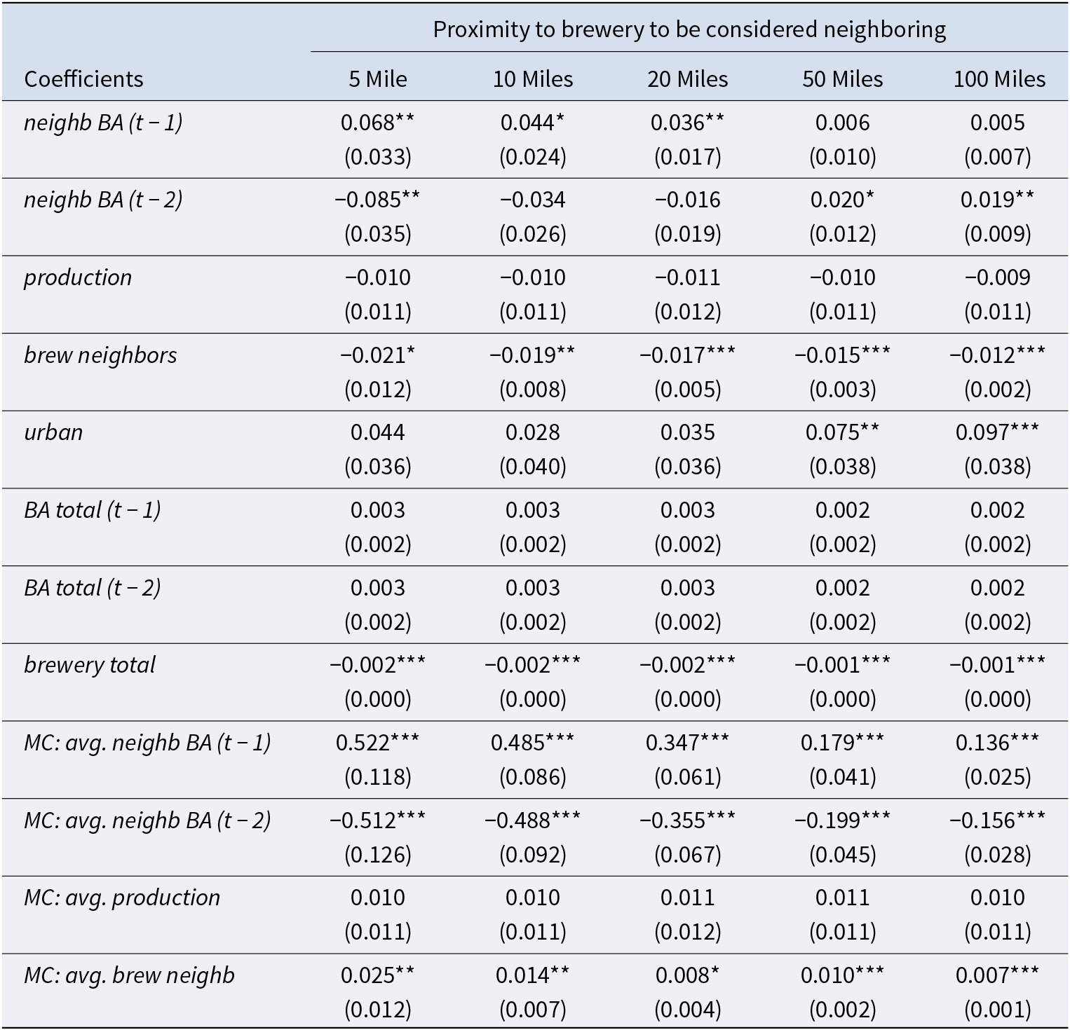
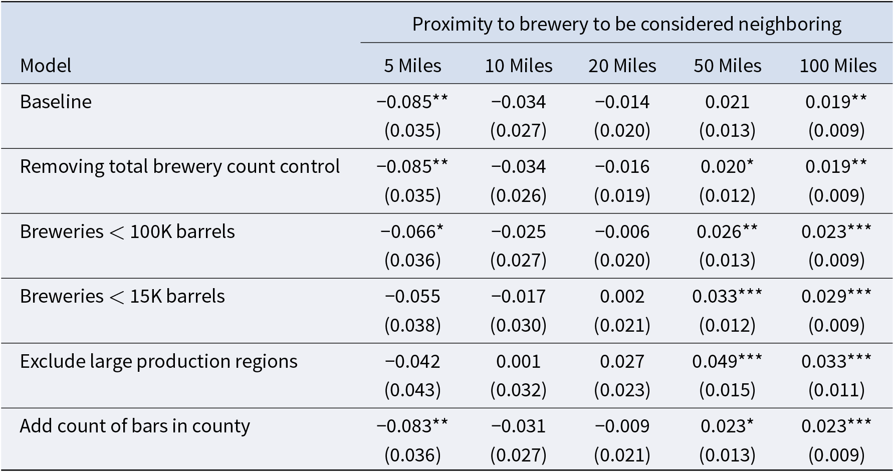
As described in Section 5.2.2, the baseline model and all robustness checks were rerun, including twice-lagged (2 years ago) regressors for neighb BA, BA total, and the brewery-averaged neighb BA for the MC device. Full results for the baseline model are in Table B1. Note that while the coefficient on neighb BA (t − 1) remains significant for the 5-, 10-, and 20-mile definitions, the coefficient on BA total (t − 1) is about halved, and both BA total coefficients are insignificant. Again, caution is warranted in interpretation due to likely multicollinearity.
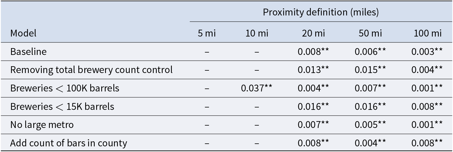
Tables B2 and B3 report the coefficient estimate of neighb BA (t − 1) and neighb BA (t − 2), respectively, for all regressions. To ease comparison, Figure B1 displays the coefficient estimates for neighb BA (t − 1) in the models that include only a year lag (solid bar), neighb BA (t − 1) in the models that include both 1- and 2-year lags (striped bar), and neighb BA (t − 2) in the models that include both 1- and 2-year lags (crosshatched bar). The patterns across all six groups are similar:
• When adding twice-lagged regressors, the once-lagged neighb BA coefficient stays the same or increases for the 5-, 10-, and 20-mile bands while shrinking to insignificance for the 50- and 100-mile bands.
• The twice-lagged neighb BA coefficient is negative, greatly so at 5 miles, while smaller for 10 and 20 miles.
• The twice-lagged neighb BA coefficient switches to positive for the 50- and 100-mile bands, while being sometimes notably greater than the once-lagged neighb BA coefficient in the original model without the twice-lagged regressors.
Table B1.Coefficient Estimates on Baseline Model (When neighb BA (t-2), BA total (t − 2), and MC: avg. Neighb BA (t − 2) Are Included as Controls)

Standard errors in parentheses.
Signif. Codes: ***: 0.01, **: 0.05, *: 0.1.
Table B2.Coefficient Estimates of neighb BA (t − 1) (nbant − 1) Under Different Models or Samples (When neighb BA (t − 2), BA total (t − 2), and MC: avg. Neighb BA (t − 2) Are Included as Controls)
Standard errors in parentheses.
Signif. Codes: ***: 0.01, **: 0.05, *: 0.1.
Table B3.Coefficient Estimates of neighb BA (t − 2) (nbant − 2) Under Different Models or Samples (When neighb BA (t − 1), BA total (t − 2), and MC: avg. Neighb BA (t − 2) Are Included as Controls)
Standard errors in parentheses.
Signif. Codes: ***: 0.01, **: 0.05, *: 0.1.


Coefficients on neighb BA for Once- and Twice-Lagged Models.

Appendix C. Robustness Check: Separate Distance Bins
Coefficient Estimates Using Separate Distance Bins

Standard errors in parentheses.
Signif. Codes: ***: 0.01, **: 0.05, *: 0.1.




 Open access

