


1. Introduction
Waves are one of the vast energy resources of the ocean. A wave energy converter (WEC) is a device that converts wave energy into electricity. Although WECs have been studied for decades, they are yet to be fully commercialised due to technical, economic and regulatory challenges. As a result, no single optimal solution has been established, and various types of WECs have been proposed, including oscillating water columns, flap-type devices, submerged pressure differential systems, point absorbers, attenuators, rotational pendulum devices, overtopping devices and gyroscopic systems. In this study, we revisit a WEC from the perspective of the interaction between ocean waves and a floating body in order to explore optimal concepts for WECs.
The study of wave–body interactions has a long history. Especially between the 1960s and 1990s, theoretical frameworks were extensively developed, and significant insights were gained. One of the most important discoveries in WECs is the theory of wave energy absorption efficiency by a floating body. For a symmetric floating body, a single mode of motion can absorb up to half of the total wave energy, and this maximum absorption occurs at the resonant frequency (Evans Reference Evans1976; Mei Reference Mei1976). This constraint occurs because the energy of the incident waves is equally distributed between symmetric and antisymmetric components (energy equally splitting law; Kato et al. Reference Kato, Kudo, Sugita and Motora1974). Therefore, by combining symmetric and antisymmetric modes of motion, it is theoretically possible to absorb all of the incident wave energy (Evans Reference Evans1976). Alternatively, perfect wave energy absorption can also be achieved in a single mode by using a floating body with asymmetric geometry (Salter Reference Salter1974). These insights have been applied to some types of WECs, such as point absorbers (Evans Reference Evans1976), oscillating water columns (Evans Reference Evans1982) and rotational pendulum-type devices (Kashiwagi, Nishimatsu & Sakai Reference Kashiwagi, Nishimatsu and Sakai2012).
In this study, we focus on a gyroscopic wave energy converter (GWEC). The GWEC is a floating body equipped with a gyroscopic power-take-off system (GPTO) as shown in figure 1. The GPTO consists of an electric generator and a flywheel mounted on a gimbal frame. The GWEC extracts energy from the precession induced by the flywheel’s rotation and the pitch motion of the floating body. Since the GPTO is enclosed within the floating body (i.e. built-in WEC, see Wang et al. Reference Wang, Sun, Xi, Dai, Xing and Xu2024), it is protected from water and waves (Salcedo et al. Reference Salcedo, Ruiz-Minguela, Rodriguez, Ricci and Santos2009), this has advantages in safety and maintenance. Furthermore, when the same size and shape of the body are used, the GWEC is expected to extract more energy than a point absorber, as its resonant period can be designed to be longer. The GWEC itself is not a novel concept; it was patented by Laithwaite & Salter (Reference Laithwaite and Salter1981) and was considered for application to Salter’s duck (Salter Reference Salter1980, Reference Salter1982). Thanks to the built-in nature of the GWEC, prototyping is relatively easy. As a result, sea trials were carried out by several independent projects, especially around 2010. In Japan, sea trials were carried out using prototypes of 5.5, 22.5 and 45 kW (Kanki et al. Reference Kanki, Morimoto, Kawanishi, Onishi and Hata2005, Reference Kanki, Arii, Furusawa and Otoyo2009). In Spain, 1/15- and 1/4-scale models were developed in the OCEANTEC WEC project, and although an absorber was not installed, tank tests and sea trials were conducted (Salcedo et al. Reference Salcedo, Ruiz-Minguela, Rodriguez, Ricci and Santos2009). In Italy, the inertial sea WEC (ISWEC) project developed 1/45-, 1/8- and full-scale prototypes, which were tested both in wave tanks and at sea (Bracco Reference Bracco2010; Bracco, Giorcelli & Mattiazzo Reference Bracco, Giorcelli and Mattiazzo2011; Cagninei et al. Reference Cagninei, Raffero, Bracco, Giorcelli, Mattiazzo and Poggi2015; Bracco et al. Reference Bracco, Cagninei, Giorcelli, Mattiazzo, Poggi and Raffero2016; Vissio Reference Vissio2017). In addition, Bracco et al. (Reference Bracco, Giorcelli, Mattiazzo, Orlando and Raffero2015) developed a hardware-in-the-loop test rig that enables the analysis of the gyroscope and generator on land. Starting from these works, various analytical studies, numerical parameter investigations and new mechanism developments have been conducted. Bracco (Reference Bracco2010) formulated the coupled equations of motion for the floating body and the gyroscope, and the relationship between body motion and power generation was clarified through linearisation of the gyroscope motion. A nonlinear analysis of the gyroscopic dynamics was conducted by Giorgi, Habib & Carapellese (Reference Giorgi, Habib and Carapellese2025). Medeiros & Brizzolara (Reference Medeiros and Brizzolara2018) performed numerical simulations using a time-domain Rankine panel method that considers the nonlinear free surface boundary condition. Khedkar et al. (Reference Khedkar, Nangia, Thirumalaisamy and Bhalla2021) also performed numerical simulations using computational fluid dynamics (CFD). A two-degree-of-freedom (2-DoF) gyroscope was proposed to enable power generation regardless of the wave direction (Bracco Reference Bracco2010; Battezzato et al. Reference Battezzato, Bracco, Giorcelli and Mattiazzo2015). A passive GWEC with geared feedback was proposed to achieve spin amplification of a flywheel without a motor (Toyoshima & Hosaka Reference Toyoshima and Hosaka2021).
Schematic diagrams of a gyroscopic WEC and its coordinate systems (defined by the right-hand rule). (a) Space-fixed (inertial) coordinate system $O$
–
$O$
– $xyz$
. Waves propagate from the negative
$xyz$
. Waves propagate from the negative $x$
-axis, and the floating body rotates around the
$x$
-axis, and the floating body rotates around the $y$
-axis with an angle
$y$
-axis with an angle $\theta$
. (b) Gimbal-fixed coordinate system
$\theta$
. (b) Gimbal-fixed coordinate system $O_g$
–
$O_g$
– $x_gy_gz_g$
. The flywheel can independently rotate around the
$x_gy_gz_g$
. The flywheel can independently rotate around the $z_g$
-axis with an angular velocity
$z_g$
-axis with an angular velocity $\dot {\psi }$
, while the gimbal can rotate around the
$\dot {\psi }$
, while the gimbal can rotate around the $x_g$
-axis with an angle
$x_g$
-axis with an angle $\varepsilon$
, together with the flywheel. The generator produces electricity in response to the rotation of this gimbal.
$\varepsilon$
, together with the flywheel. The generator produces electricity in response to the rotation of this gimbal.

In many previous analytical studies, the performance of the GWEC has been analysed by assuming constant floating body motions as external inputs. However, in reality, the situation is more complex: waves excite the motion of the floating body, which in turn induces the gyroscope motion and power generation. This creates a feedback loop that alters the floating body motion and consequently changes the radiated waves. Therefore, it is essential to consider the coupled interactions among the waves, the floating body and the gyroscope. So far, coupled fluid dynamics analyses of waves, the floating body and the gyroscope have been limited to numerical simulations and associated parameter studies. Overall, there is a lack of fundamental analytical knowledge of the wave–body–gyroscope interaction relative to the progress made in applied development.
Therefore, in this study, we return to the tradition of this field and conduct a coupled theoretical analysis of waves, the floating body and the gyroscope in the GWEC. We aim to reveal the fundamental characteristics of the GWEC and determine the optimal control parameters. The waves are assumed to be regular waves propagating unidirectionally over an infinitely deep ocean across all wave frequencies, and the GWEC is modelled as a 1-DoF system with pitch motion. In addition, the power take-off system is modelled as a linear spring–damper system. Accordingly, we simplify the problem to two dimensions and linearise the gyroscope model by assuming small-amplitude periodic oscillations around its equilibrium position. Based on this, the problem is formulated in the frequency domain. Various hydrodynamic relations involving the waves and the floating body are taken into account to determine the maximum energy absorption efficiency of the GWEC. Under this condition, the optimal control parameters of the GWEC, namely, the rotational speed of the flywheel and the spring and damping coefficients of the generator, are also identified. Although the methodologies themselves are classical, the findings derived from them are highly significant: the GWEC can achieve the maximum theoretical energy absorption efficiency of 1/2 at any wave frequency within the framework of linear theory, as the flywheel’s rotational speed provides an additional degree of controllability.
To verify the theory derived in this study, numerical simulations are performed in both the frequency and time domains by assuming linearised motion of the gyroscope. The floating body is modelled based on a prototype that will be used in future small-scale tank tests. In addition, time-domain numerical simulations incorporating the nonlinear gyroscopic response are also performed to clarify the limitations of the proposed linear gyroscopic model. This study addresses the current lack of fundamental theoretical analyses of the GWEC by developing a wave–body–gyroscope interaction theory and identifying the optimal parameters for maximising energy absorption. Our findings provide valuable insights that can guide the future design of WECs.
2. Theory
2.1. Problem statement and coordinate systems
We consider a GWEC, which consists of a floating body equipped with a GPTO, as described in figure 1(a). In the GPTO, a flywheel is mounted on a gimbal frame, and the gimbal is connected to an electric generator (see figure 1 b). When the floating body oscillates in response to waves while the flywheel is rotating, a gyroscopic moment is caused. This moment drives the gimbal to rotate, and this rotation is then converted into electricity by the generator. This is the principle of the GWEC.
As shown in figure 1, space-fixed and gimbal-fixed coordinate systems are defined based on the right-hand rule, where the positive rotation direction follows the right-hand screw convention. The three-dimensional space-fixed (inertial) coordinate system $O$
–
$O$
– $xyz$
is defined, with the origin
$xyz$
is defined, with the origin $O$
located at the centre of gravity of the floating body in its equilibrium position. The
$O$
located at the centre of gravity of the floating body in its equilibrium position. The $z$
-axis is defined as positive in the upward vertical direction. A sea depth is assumed infinite, and thus deep-water waves are considered. Waves are incident from the negative
$z$
-axis is defined as positive in the upward vertical direction. A sea depth is assumed infinite, and thus deep-water waves are considered. Waves are incident from the negative $x$
-axis. The wave amplitude is small enough compared with the wavelength. In addition, the fluid is assumed incompressible and inviscid, and the flow motion is irrotational. As a result, the problem can be discussed under the linear potential flow theory. To simplify the problem, only the rotational motions (roll, pitch and yaw) of the floating body are considered, and translational motions (surge, sway and heave) are neglected. A drift of the floating body is also not considered as the drift force will be cancelled by a mooring system, although such a mooring is not modelled in the present problem. The rotational angles corresponding to the
$x$
-axis. The wave amplitude is small enough compared with the wavelength. In addition, the fluid is assumed incompressible and inviscid, and the flow motion is irrotational. As a result, the problem can be discussed under the linear potential flow theory. To simplify the problem, only the rotational motions (roll, pitch and yaw) of the floating body are considered, and translational motions (surge, sway and heave) are neglected. A drift of the floating body is also not considered as the drift force will be cancelled by a mooring system, although such a mooring is not modelled in the present problem. The rotational angles corresponding to the $x$
-,
$x$
-, $y$
- and
$y$
- and $z$
-axes are denoted by
$z$
-axes are denoted by $\varphi$
(roll),
$\varphi$
(roll), $\theta$
(pitch) and
$\theta$
(pitch) and $\gamma$
(yaw), respectively.
$\gamma$
(yaw), respectively.
The gimbal-fixed coordinate system $O_g$
–
$O_g$
– $x_gy_gz_g$
is also considered, where the origin
$x_gy_gz_g$
is also considered, where the origin $O_g$
is defined to coincide with the centres of rotation of both the flywheel and the gimbal. Moreover, we assume the origin
$O_g$
is defined to coincide with the centres of rotation of both the flywheel and the gimbal. Moreover, we assume the origin $O_g$
coincides with the origin
$O_g$
coincides with the origin $O$
. The GPTO rotates around the
$O$
. The GPTO rotates around the $y_g$
-axis due to waves, and its rotation angle coincides with the pitch angle
$y_g$
-axis due to waves, and its rotation angle coincides with the pitch angle $\theta$
of the floating body. The gimbal rotates around the
$\theta$
of the floating body. The gimbal rotates around the $x_g$
-axis by an angle
$x_g$
-axis by an angle $\varepsilon$
, together with the flywheel, while the flywheel independently rotates around the
$\varepsilon$
, together with the flywheel, while the flywheel independently rotates around the $z_g$
-axis by an angle
$z_g$
-axis by an angle $\psi$
. The generator produces electricity in response to the rotation of this gimbal. Using the
$\psi$
. The generator produces electricity in response to the rotation of this gimbal. Using the $y$
–
$y$
– $x$
Euler angles, the relationship between the space-fixed coordinate system and the gimbal-fixed coordinate system is given as follows:
$x$
Euler angles, the relationship between the space-fixed coordinate system and the gimbal-fixed coordinate system is given as follows:
 \begin{eqnarray} \left (\begin{array}{c} x_g\\ y_g\\ z_g \end{array}\right )&=& \left (\begin{array}{ccc} 1&0&0\\ 0&\cos \varepsilon &\sin \varepsilon \\ 0&-\sin \varepsilon &\cos \varepsilon \end{array}\right )\left (\begin{array}{ccc} \cos \theta &0&-\sin \theta \\ 0&1&0\\ \sin \theta &0&\cos \theta \end{array}\right )\left (\begin{array}{c} x\\ y\\ z \end{array}\right )\nonumber \\ &=& \left (\begin{array}{ccc} \cos \theta &0&-\sin \theta \\ \sin \varepsilon \sin \theta &\cos \varepsilon &\sin \varepsilon \cos \theta \\ \cos \varepsilon \sin \theta &-\sin \varepsilon &\cos \varepsilon \cos \theta \end{array}\right )\left (\begin{array}{c} x\\ y\\ z \end{array}\right )\! .\end{eqnarray}
2.2. Equations of motion of the GWEC
At first, we consider equations of motion of the gyroscope (consisting of the flywheel and gimbal) on the gimbal-fixed system. A principal moment of inertia of the gimbal is assumed negligible (i.e. $\boldsymbol{I}_{\!\textit{gim}}\approx 0$
), and thus a principal moment of inertia of the gyroscope is given by that of the flywheel, as
$\boldsymbol{I}_{\!\textit{gim}}\approx 0$
), and thus a principal moment of inertia of the gyroscope is given by that of the flywheel, as
 \begin{eqnarray} \boldsymbol {I}_{{g}}\approx \boldsymbol {I}_{{f}}= \left (\begin{array}{ccc} I&0&0\\ 0&I&0\\ 0&0&J \end{array}\right )\! ,\end{eqnarray}
where subscripts $\textrm {gim}$
,
$\textrm {gim}$
, $\textrm {g}$
and
$\textrm {g}$
and $\textrm {f}$
denote quantities of the gimbal, gyroscope and flywheel, respectively. Note that inertial moments are designed as
$\textrm {f}$
denote quantities of the gimbal, gyroscope and flywheel, respectively. Note that inertial moments are designed as $I\leqslant J$
in typical GWEC (Bracco Reference Bracco2010; Khedkar et al. Reference Khedkar, Nangia, Thirumalaisamy and Bhalla2021). Angular velocity vectors of the gimbal and flywheel are obtained as (see Bracco Reference Bracco2010)
$I\leqslant J$
in typical GWEC (Bracco Reference Bracco2010; Khedkar et al. Reference Khedkar, Nangia, Thirumalaisamy and Bhalla2021). Angular velocity vectors of the gimbal and flywheel are obtained as (see Bracco Reference Bracco2010)
 \begin{eqnarray} \boldsymbol{\omega }_{\textit{gim}}= \left (\begin{array}{c} \dot {\varepsilon }\\ \dot {\theta }\cos \varepsilon \\ -\dot {\theta }\sin \varepsilon \end{array}\right ),\; \boldsymbol{\omega }_{{f}}= \left (\begin{array}{c} \dot {\varepsilon }\\ \dot {\theta }\cos \varepsilon \\ -\dot {\theta }\sin \varepsilon +\dot {\psi } \end{array}\right )\! .\end{eqnarray}
Therefore, angular momentum $\boldsymbol {L}_{{g}}$
of the gyroscope and its time derivative are written as
$\boldsymbol {L}_{{g}}$
of the gyroscope and its time derivative are written as
 \begin{align} \boldsymbol {L}_{{g}}= \boldsymbol {I}_{{f}} \boldsymbol{\omega }_{{f}}+\boldsymbol {I}_{\textit{gim}} \boldsymbol{\omega }_{\textit{gim}}= \left (\begin{array}{c} I\dot {\varepsilon }\\ I\dot {\theta }\cos \varepsilon \\ J(-\dot {\theta }\sin \varepsilon +\dot {\psi }) \end{array}\right )\! ,\end{align}
 \begin{align} \frac {{\rm d}\boldsymbol {L}_{{g}}}{{\rm d}t}=\frac {\delta \boldsymbol {L}_{{g}}}{\delta t}+\boldsymbol{\omega }_{\textit{gim}}\times \boldsymbol {L}_{{g}} = \left (\begin{array}{c} I\ddot {\varepsilon }+(I-J)\dot {\theta }^2\cos \varepsilon \sin \varepsilon +J\dot {\theta }\dot {\psi }\cos \varepsilon \\ I\ddot {\theta }\cos \varepsilon +(J-2I)\dot {\varepsilon }\dot {\theta }\sin \varepsilon -J\dot {\varepsilon }\dot {\psi }\\ J(-\ddot {\theta }\sin \varepsilon -\dot {\varepsilon }\dot {\theta }\cos \varepsilon +\ddot {\psi }) \end{array}\right )\! .\end{align}
The torques acting on the gyroscope are defined as $\boldsymbol {T}_{{g}}|_g=(T_{\textit{PTO}}|_g, T_{\textit{bg}}|_g, T_{{f}}|_g)$
, where
$\boldsymbol {T}_{{g}}|_g=(T_{\textit{PTO}}|_g, T_{\textit{bg}}|_g, T_{{f}}|_g)$
, where $|_g$
represents quantities on the gimbal-fixed system,
$|_g$
represents quantities on the gimbal-fixed system, $T_{\textit{PTO}}|_g$
is the torque that rotates the generator,
$T_{\textit{PTO}}|_g$
is the torque that rotates the generator, $T_{\textit{bg}}|_g$
is the contact moment between the floating body and the gyroscope and
$T_{\textit{bg}}|_g$
is the contact moment between the floating body and the gyroscope and $T_{{f}}|_g$
is the torque that rotates the flywheel. As a result, Euler’s rotation equations of the gyroscope are given as
$T_{{f}}|_g$
is the torque that rotates the flywheel. As a result, Euler’s rotation equations of the gyroscope are given as
 \begin{eqnarray} \frac {{\rm d}\boldsymbol {L}_{{g}}}{{\rm d}t}=\boldsymbol {T}_{{g}}|_g \to \left (\begin{array}{c} I\ddot {\varepsilon }+(I-J)\dot {\theta }^2\cos \varepsilon \sin \varepsilon +J\dot {\theta }\dot {\psi }\cos \varepsilon \\ I\ddot {\theta }\cos \varepsilon +(J-2I)\dot {\varepsilon }\dot {\theta }\sin \varepsilon -J\dot {\varepsilon }\dot {\psi }\\ J(-\ddot {\theta }\sin \varepsilon -\dot {\varepsilon }\dot {\theta }\cos \varepsilon +\ddot {\psi }) \end{array}\right ) = \left (\!\begin{array}{c} T_{\textit{PTO}}|_g\\ T_{\textit{bg}}|_g\\ T_{{f}}|_g \end{array}\!\right )\! .\end{eqnarray}
It should be mentioned that this equation appears to differ from the formulation used by the ISWEC group (Bracco Reference Bracco2010; Bracco et al. Reference Bracco, Cagninei, Giorcelli, Mattiazzo, Poggi and Raffero2016). This is because they define their space-fixed coordinate system such that waves propagate from the negative direction of the $y$
-axis, whereas we use the
$y$
-axis, whereas we use the $x$
-axis. Aside from this difference, the two formulations are equivalent.
$x$
-axis. Aside from this difference, the two formulations are equivalent.
Secondly, equations of motion of the floating body are formulated. The moment of inertia $\boldsymbol {I}_{{b}}$
of the floating body is represented by
$\boldsymbol {I}_{{b}}$
of the floating body is represented by
 \begin{eqnarray} \boldsymbol {I}_{{b}}= \left (\begin{array}{ccc} I_{44}&0&I_{46}\\ 0&I_{55}&0\\ I_{64}&0&I_{66} \end{array}\right )\! ,\end{eqnarray}
where the subscript $\textrm {b}$
denotes the quantities of the floating body. Note that translational motions are assigned to mode numbers 1, 2 and 3, while rotational motions are assigned to mode numbers 4, 5 and 6. Although only rotational motions are considered in this study, translational motions will appear later (in § 2.3). Based on the law of action and reaction, the torque in (2.6) also acts on the floating body. The torques on the space-fixed coordinate system are calculated by (2.1)as
$\textrm {b}$
denotes the quantities of the floating body. Note that translational motions are assigned to mode numbers 1, 2 and 3, while rotational motions are assigned to mode numbers 4, 5 and 6. Although only rotational motions are considered in this study, translational motions will appear later (in § 2.3). Based on the law of action and reaction, the torque in (2.6) also acts on the floating body. The torques on the space-fixed coordinate system are calculated by (2.1)as
 \begin{eqnarray} \boldsymbol {T}_{{g}}&=& \left (\begin{array}{ccc} \cos \theta &0&\sin \theta \\ 0&1&0\\ -\sin \theta &0&\cos \theta \end{array}\right ) \left (\begin{array}{ccc} 1&0&0\\ 0&\cos \varepsilon &-\sin \varepsilon \\ 0&\sin \varepsilon &\cos \varepsilon \end{array}\right ) \boldsymbol {T}_{{g}}|_g\nonumber \\ &=&\left (\begin{array}{c} T_{\textit{PTO}}|_g\cos \theta +T_{\textit{bg}}|_g\sin \theta \sin \varepsilon +T_{{f}}|_g\sin \theta \cos \varepsilon \\ T_{\textit{bg}}|_g\cos \varepsilon -T_{{f}}|_g\sin \varepsilon \\ -T_{\textit{PTO}}|_g\sin \theta +T_{\textit{bg}}|_g\cos \theta \sin \varepsilon +T_{{f}}|_g\cos \theta \cos \varepsilon \end{array}\right ). \end{eqnarray}
In addition, the linearised hydrodynamic forces are given by Cummins (Reference Cummins1962) as
 \begin{eqnarray} &&\boldsymbol {F}_{\textit{hydro}}^G=\boldsymbol {F}_{\textit{rad}}^G+\boldsymbol {F}_{ {sta}}^G+\boldsymbol {F}_{ {\textit{ex}}}^G\nonumber \\ &&=\left (\begin{array}{c} \displaystyle -a_{44,\infty }^G\ddot {\varphi }-a_{46,\infty }^G\ddot {\gamma }-\int _{-\infty }^t L_{44}^G(t-\tau )\dot {\varphi }(\tau ){\rm d}\tau -\int _{-\infty }^t L_{46}^G(t-\tau )\dot {\gamma }(\tau ){\rm d}\tau \\ \displaystyle -a_{55,\infty }^G\ddot {\theta }-\int _{-\infty }^t L_{55}^G(t-\tau )\dot {\theta }(\tau ){\rm d}\tau \\ \displaystyle -a_{64,\infty }^G\ddot {\varphi }-a_{66,\infty }^G\ddot {\gamma }-\int _{-\infty }^t L_{64}^G(t-\tau )\dot {\varphi }(\tau ){\rm d}\tau -\int _{-\infty }^t L_{66}^G(t-\tau )\dot {\gamma }(\tau ){\rm d}\tau \end{array}\right )\nonumber \\ &&\quad + \left (\begin{array}{c} \displaystyle -c_{44}^G\varphi \\ \displaystyle -c_{55}^G\theta \\ \displaystyle 0 \end{array}\right ) + \left (\begin{array}{c} 0\\ f_{5}^G\\ 0 \end{array}\right )\! ,\end{eqnarray}
where the superscript $G$
represents the quantities around the centre of gravity. Here,
$G$
represents the quantities around the centre of gravity. Here, $\boldsymbol {F}_{\textit{rad}}^G$
is the radiation force, consisting of the added mass
$\boldsymbol {F}_{\textit{rad}}^G$
is the radiation force, consisting of the added mass $a_{ij,\infty }^G$
at wave frequency
$a_{ij,\infty }^G$
at wave frequency $\omega \to \infty$
, and the memory effect function (also known as the retardation function)
$\omega \to \infty$
, and the memory effect function (also known as the retardation function) $L_{ij}^G(t)$
(
$L_{ij}^G(t)$
( $i,j=4,5,6$
). Also,
$i,j=4,5,6$
). Also, $\boldsymbol {F}_{{sta}}^G$
is the hydrostatic force;
$\boldsymbol {F}_{{sta}}^G$
is the hydrostatic force; $c_{ii}^G$
(
$c_{ii}^G$
( $i=4,5$
) is the restoring coefficient. Moreover,
$i=4,5$
) is the restoring coefficient. Moreover, $\boldsymbol {F}_{{\textit{ex}}}^G$
is the wave exciting force where
$\boldsymbol {F}_{{\textit{ex}}}^G$
is the wave exciting force where $f_5^G$
is the moment along the pitch direction. Therefore, the equation of motion of the floating body is given as
$f_5^G$
is the moment along the pitch direction. Therefore, the equation of motion of the floating body is given as
 \begin{eqnarray} \boldsymbol {I}_{{b}}\ddot {\boldsymbol{\chi }}=\boldsymbol {F}_{\textit{hydro}}^G-\boldsymbol {T}_{{g}} ,\end{eqnarray}
where $\boldsymbol{\chi }=(\varphi , \theta , \gamma )$
. Equation (2.10) indicates that roll and yaw motions are induced by the gyroscopic moment whereas wave excitation is only for the pitch direction. However, these motions will be cancelled by a mooring system in practice (Khedkar et al. Reference Khedkar, Nangia, Thirumalaisamy and Bhalla2021). Therefore, we only consider the pitch motion of the floating body as
$\boldsymbol{\chi }=(\varphi , \theta , \gamma )$
. Equation (2.10) indicates that roll and yaw motions are induced by the gyroscopic moment whereas wave excitation is only for the pitch direction. However, these motions will be cancelled by a mooring system in practice (Khedkar et al. Reference Khedkar, Nangia, Thirumalaisamy and Bhalla2021). Therefore, we only consider the pitch motion of the floating body as
 \begin{align} \left(I_{55}+a_{55,\infty }^G\right)\ddot {\theta }+\int _{-\infty }^t L_{55}^G(t-\tau )\dot {\theta }(\tau ){\rm d}\tau +c_{55}^G\theta =f_5^G-T_{\textit{bg}}|_g\cos \varepsilon +T_{{f}}|_g\sin \varepsilon .\end{align}
Coupling (2.6) and (2.11), the equations of motion of the floating body and the gyroscope are given as
 \begin{align} &\left (\begin{array}{ccc} I&0&0\\ 0&I_{55}+a^G_{55,\infty }+I\cos ^2\varepsilon +J\sin ^2\varepsilon &-J\sin \varepsilon \\ 0&-J\sin \varepsilon &J \end{array}\right ) \left (\begin{array}{c} \ddot {\varepsilon }\\ \ddot {\theta }\\ \ddot {\psi } \end{array}\right )\nonumber \\ &=\left (\begin{array}{c} \displaystyle -(I-J)\dot {\theta }^2\cos \varepsilon \sin \varepsilon -J\dot {\theta }\dot {\psi }\cos \varepsilon +T_{\textit{PTO}}|_g\\ \displaystyle -\int _{-\infty }^t L_{55}^G(t-\tau )\dot {\theta }(\tau ){\rm d}\tau -c_{55}^G\theta +f_5^G-2(J-I)\dot {\varepsilon }\dot {\theta }\sin \varepsilon \cos \varepsilon +J\dot {\varepsilon }\dot {\psi }\cos \varepsilon \\ \displaystyle J\dot {\varepsilon }\dot {\theta }\cos \varepsilon + T_{{f}}|_g \end{array}\right ). \end{align}
Here, the generator is modelled by a linear spring–damper system to generate electricity through periodic oscillations of the shaft around the equilibrium angle (Bracco Reference Bracco2010), which is represented as
 \begin{eqnarray} T_{\textit{PTO}}|_g=-k_{{g}}\varepsilon -c_{{g}}\dot {\varepsilon } ,\end{eqnarray}
where $k_{{g}}$
is the spring coefficient (stiffness) and
$k_{{g}}$
is the spring coefficient (stiffness) and $c_{{g}}$
is the damping coefficient. Moreover, we assume the rotation speed of the flywheel is constant
$c_{{g}}$
is the damping coefficient. Moreover, we assume the rotation speed of the flywheel is constant $\dot {\psi }=\textrm {const.}$
(i.e.
$\dot {\psi }=\textrm {const.}$
(i.e. $\ddot {\psi }=0$
) for the simplification of the problem. As a result, (2.12) becomes
$\ddot {\psi }=0$
) for the simplification of the problem. As a result, (2.12) becomes
 \begin{align} &\left (\begin{array}{cc} I&0\\ 0&I_{55}+a^G_{55,\infty }+I\cos ^2\varepsilon +J\sin ^2\varepsilon \\ \end{array}\right ) \left (\begin{array}{c} \ddot {\varepsilon }\\ \ddot {\theta } \end{array}\right )\nonumber \\ &=\left (\begin{array}{c} \displaystyle -(I-J)\dot {\theta }^2\cos \varepsilon \sin \varepsilon -J\dot {\theta }\dot {\psi }\cos \varepsilon -k_{{g}}\varepsilon -c_{{g}}\dot {\varepsilon }\\ \displaystyle -\int _{-\infty }^t L_{55}^G(t-\tau )\dot {\theta }(\tau ){\rm d}\tau -c_{55}^G\theta +f_5^G-2(J-I)\dot {\varepsilon }\dot {\theta }\sin \varepsilon \cos \varepsilon +J\dot {\varepsilon }\dot {\psi }\cos \varepsilon \end{array}\right )\! .\end{align}
By solving (2.14), the motions of the floating body and the gyroscope can be obtained. It should be mentioned that the gyroscopic moment becomes zero at $\varepsilon =\pm \pi /2$
, i.e. a gimbal lock appears. Note that consistency in the case of zero flywheel speed is verified in Appendix A.1.
$\varepsilon =\pm \pi /2$
, i.e. a gimbal lock appears. Note that consistency in the case of zero flywheel speed is verified in Appendix A.1.
2.3. Linearisation and time variable separation of the equations of motion
To understand the characteristics of the GWEC, we linearise the equation of motion (2.14) around its equilibrium angle $\varepsilon =0$
(Bracco Reference Bracco2010). Assuming a small angle of
$\varepsilon =0$
(Bracco Reference Bracco2010). Assuming a small angle of $\varepsilon$
, (2.14) is linearised as
$\varepsilon$
, (2.14) is linearised as
 \begin{eqnarray} \left \{\!\! \begin{array}{l} \displaystyle I\ddot {\varepsilon }+c_{{g}}\dot {\varepsilon }+k_{{g}}\varepsilon +J\dot {\psi }\dot {\theta }=0,\\ \displaystyle \left(I_{55}+a^G_{55,\infty }+I\right)\ddot {\theta }+\int _{-\infty }^t L_{55}^G(t-\tau )\dot {\theta }(\tau ){\rm d}\tau +c_{55}^G\theta -J\dot {\psi }\dot {\varepsilon }=f_5^G .\end{array}\right . \end{eqnarray}
We consider a case where the motions of the GWEC are periodic in response to regular waves with a monochromatic frequency $\omega$
. Then, the time variables can be separated as follows:
$\omega$
. Then, the time variables can be separated as follows:
 \begin{eqnarray} \varepsilon =\textrm {Re}[\mathcal{E} e^{i\omega t}],\;\theta =\textrm {Re}[\varTheta e^{i\omega t}],\; f_5^G=\textrm {Re}[E_5^Ge^{i\omega t}] ,\end{eqnarray}
where $\mathcal{E}$
,
$\mathcal{E}$
, $\varTheta$
and
$\varTheta$
and $E_5^G$
are the complex amplitudes of the gyroscope motion, the motion of the floating body and the wave exciting force. Applying the Fourier transform to (2.15), we get equations of motion in the frequency domain as
$E_5^G$
are the complex amplitudes of the gyroscope motion, the motion of the floating body and the wave exciting force. Applying the Fourier transform to (2.15), we get equations of motion in the frequency domain as
 \begin{eqnarray} \left \{\!\! \begin{array}{l} \displaystyle (-\omega ^2I+i\omega c_{{g}} +k_{{g}})\mathcal{E}+i\omega J\dot {\psi }\varTheta =0,\\[2pt] \left[-\omega ^2\left(I_{55}+a_{55}^G+I\right)+i\omega b_{55}^G+c_{55}^G\right]\varTheta -i\omega J\dot {\psi }\mathcal{E}=E_5^G ,\end{array}\right . \end{eqnarray}
where $a_{55}^G$
and
$a_{55}^G$
and $b_{55}^G$
are the added mass and wave-making damping coefficient around the centre of gravity. Note that the restoring coefficient is
$b_{55}^G$
are the added mass and wave-making damping coefficient around the centre of gravity. Note that the restoring coefficient is $c_{55}^G=\rho g \boldsymbol{\nabla }\overline {\textrm {GM}}$
, where
$c_{55}^G=\rho g \boldsymbol{\nabla }\overline {\textrm {GM}}$
, where $\boldsymbol{\nabla}$
is the displacement and
$\boldsymbol{\nabla}$
is the displacement and $\overline {\textrm {GM}}$
is the metacentric height.
$\overline {\textrm {GM}}$
is the metacentric height.
For regular waves, the power of incident waves is given as (see Mei, Stiassnie & Yue Reference Mei, Stiassnie and Yue2005)
 \begin{eqnarray} P_{{W}}=\frac {1}{2}\rho g \zeta _{{a}}^2v_g=\frac {\rho g^2\zeta _{{a}}^2}{4\omega } ,\end{eqnarray}
where $\rho$
is the fluid density,
$\rho$
is the fluid density, $g$
is the gravitational acceleration,
$g$
is the gravitational acceleration, $\zeta _{{a}}$
is the amplitude of incident waves and
$\zeta _{{a}}$
is the amplitude of incident waves and $v_g=g/(2\omega )$
is the group velocity of deep-water waves. On the other hand, the extracted power by the GPTO is estimated as
$v_g=g/(2\omega )$
is the group velocity of deep-water waves. On the other hand, the extracted power by the GPTO is estimated as
 \begin{eqnarray} P_{\textit{PTO}}=\frac {1}{T}\int _0^Tc_{{g}}\dot {\varepsilon }^2{\rm d}t=\frac {1}{2}c_{{g}}\omega ^2 |\mathcal{E}|^2 .\end{eqnarray}
As a result, energy absorption efficiency is described as
 \begin{eqnarray} \eta =\frac {P_{\textit{PTO}}}{P_{{W}}}=\frac {2c_{{g}}\omega ^3|\mathcal{E}|^2}{\rho g^2 \zeta _{{a}}^2} .\end{eqnarray}
2.4. Maximum energy absorption efficiency and optimal control parameters
The purpose of this paper is to understand the fundamental characteristics of the GWEC. We are particularly interested in its energy absorption performance. To analyse this, we reduce the three-dimensional problem to a two-dimensional one in the $O$
–
$O$
– $xz$
plane, i.e. the cross-section at
$xz$
plane, i.e. the cross-section at $y=0$
. Then, the classical two-dimensional hydrodynamic approach can be applied based on the linear potential flow theory (e.g. Mei et al. Reference Mei, Stiassnie and Yue2005; Newman Reference Newman2018). The velocity potential is defined as
$y=0$
. Then, the classical two-dimensional hydrodynamic approach can be applied based on the linear potential flow theory (e.g. Mei et al. Reference Mei, Stiassnie and Yue2005; Newman Reference Newman2018). The velocity potential is defined as
 \begin{eqnarray} \displaystyle \varPhi (x,z,t)=\textrm {Re}\left [\left \{\frac {ig \zeta _{{a}}}{\omega }(\varphi _0+\varphi _7)+i\omega \varTheta \varphi _5\right \} e^{i\omega t}\right ] ,\end{eqnarray}
where $\varphi _0$
,
$\varphi _0$
, $\varphi _7$
and
$\varphi _7$
and $\varphi _5$
are the complex amplitudes of the velocity potential of the incident waves, the scattering waves and the radiation of the pitch mode, respectively. These velocity potentials are solutions to the Laplace equation, subject to the boundary conditions of the linearised free surface, the sea bottom, the body surface and the radiation in the far field. Generally, the velocity potential and its relevant quantities are defined at the point on the mean surface. However, we consider the pitch motion of the GWEC around the centre of gravity. The velocity potential of the pitch mode around the centre of gravity is given as
$\varphi _5$
are the complex amplitudes of the velocity potential of the incident waves, the scattering waves and the radiation of the pitch mode, respectively. These velocity potentials are solutions to the Laplace equation, subject to the boundary conditions of the linearised free surface, the sea bottom, the body surface and the radiation in the far field. Generally, the velocity potential and its relevant quantities are defined at the point on the mean surface. However, we consider the pitch motion of the GWEC around the centre of gravity. The velocity potential of the pitch mode around the centre of gravity is given as
 \begin{eqnarray} \displaystyle \varphi _5^G=\varphi _5-\ell _G \varphi _1 ,\end{eqnarray}
where $\ell _G(\gt 0)$
is the vertical distance between the centre of gravity and the mean surface of the water, and
$\ell _G(\gt 0)$
is the vertical distance between the centre of gravity and the mean surface of the water, and $\varphi _1$
is the velocity potential of the surge mode. Accordingly, quantities (such as the added mass and damping coefficient) are calculated by this velocity potential.
$\varphi _1$
is the velocity potential of the surge mode. Accordingly, quantities (such as the added mass and damping coefficient) are calculated by this velocity potential.
Here, we consider the progressive waves radiated outward from the floating body. The velocity potential of such waves is represented as
 \begin{eqnarray} \displaystyle \varphi _j^G \simeq iH_j^{G,\pm } e^{Kz\mp iKx} \quad \textrm {as}\; x\to \pm \infty ,\end{eqnarray}
where $K$
is the wavenumber that satisfies the deep-water dispersion relation
$K$
is the wavenumber that satisfies the deep-water dispersion relation $K=\omega ^2/g$
. In addition,
$K=\omega ^2/g$
. In addition, $H_j^{G,\pm }$
is the Kochin function (Kochin Reference Kochin1951), defined as
$H_j^{G,\pm }$
is the Kochin function (Kochin Reference Kochin1951), defined as
 \begin{eqnarray} \displaystyle H_j^{G,\pm }=\int _{S_H}\left (\frac {\partial \varphi ^G_j}{\partial n}-\varphi ^G_j \frac {\partial }{\partial n}\right )e^{K\zeta \pm iK\xi }{\rm d}\ell ,\end{eqnarray}
where $S_H$
is the surface of the floating body. The radiated waves propagating in the positive
$S_H$
is the surface of the floating body. The radiated waves propagating in the positive $x$
-direction are denoted by the superscript
$x$
-direction are denoted by the superscript $+$
, while those propagating in the negative
$+$
, while those propagating in the negative $x$
-direction are denoted by
$x$
-direction are denoted by $-$
. Using the Kochin function, the reflection and transmission coefficients are given as
$-$
. Using the Kochin function, the reflection and transmission coefficients are given as
 \begin{align} &\qquad\qquad R=iH_7^-,\; T=1+iH_7^+ , \end{align}
 \begin{align} & C_R=R+iK\frac {\varTheta }{\zeta _{{a}}}H_5^{G,-},\; C_T=T+iK\frac {\varTheta }{\zeta _{{a}}}H_5^{G,+} , \end{align}
where $R$
and
$R$
and $T$
are the reflection and transmission coefficients in the diffraction problem, while
$T$
are the reflection and transmission coefficients in the diffraction problem, while $C_R$
and
$C_R$
and $C_T$
are those in the free-motion problem.
$C_T$
are those in the free-motion problem.
We consider the case where the geometry of the floating body is symmetric with respect to the $z$
-axis. Then, based on the Bessho–Newman relation (Bessho Reference Bessho1965; Newman Reference Newman1975), the reflection and transmission coefficients (2.25) in the diffraction problem are deformed as
$z$
-axis. Then, based on the Bessho–Newman relation (Bessho Reference Bessho1965; Newman Reference Newman1975), the reflection and transmission coefficients (2.25) in the diffraction problem are deformed as
 \begin{align} & R=\frac {1}{2}\left (\frac {H_3^+}{\overline {H}_3^+}+\frac {H_5^{G,+}}{\overline {H}_5^{G,+}}\right )\! , \end{align}
 \begin{align} &T=\frac {1}{2}\left (\frac {H_3^+}{\overline {H}_3^+}-\frac {H_5^{G,+}}{\overline {H}_5^{G,+}}\right )\! .\end{align}
Here, the overline represents the complex conjugate of a function. Radiated waves can be separated into symmetric and antisymmetric components. Using (2.25) to (2.28), symmetric component $\mathcal{A}$
and antisymmetric component
$\mathcal{A}$
and antisymmetric component $\mathcal{B}$
are calculated as
$\mathcal{B}$
are calculated as
 \begin{align} &\qquad\quad \mathcal{A}=\frac {1}{2}(C_R+C_T)=\frac {1}{2}\frac {H_3^+}{\overline {H}_3^+} , \end{align}
 \begin{align} & \mathcal{B}=\frac {1}{2}(C_R-C_T)=\frac {1}{2}\frac {H_5^{G,+}}{\overline {H}_5^{G,+}} -iK\frac {\varTheta }{\zeta _{{a}}}H_5^{G,+} . \end{align}
Equation (2.29) indicates that the symmetric component is irrelevant to the pitch motion ( $j=5$
). When the symmetric body geometry is considered, the incident wave energy is equally distributed between the symmetric and antisymmetric components (energy equally splitting law; Kato et al. Reference Kato, Kudo, Sugita and Motora1974; Murashige & Kinoshita Reference Murashige and Kinoshita1991). As a result, it is known that the maximum energy absorbed by a one-degree-of-freedom (1-DoF) symmetric body is half of the incident wave energy (Evans Reference Evans1976; Mei Reference Mei1976), i.e. the energy absorption efficiency is
$j=5$
). When the symmetric body geometry is considered, the incident wave energy is equally distributed between the symmetric and antisymmetric components (energy equally splitting law; Kato et al. Reference Kato, Kudo, Sugita and Motora1974; Murashige & Kinoshita Reference Murashige and Kinoshita1991). As a result, it is known that the maximum energy absorbed by a one-degree-of-freedom (1-DoF) symmetric body is half of the incident wave energy (Evans Reference Evans1976; Mei Reference Mei1976), i.e. the energy absorption efficiency is $\eta =1/2$
.
$\eta =1/2$
.
We consider the case where all the energy of the antisymmetric component (2.30) is absorbed by the GWEC. For simplicity, we hereafter write the conservative terms as $I-k_{{g}}/\omega ^2\equiv I_{{g}}$
and
$I-k_{{g}}/\omega ^2\equiv I_{{g}}$
and $(I_{55}+a_{55}^G+I)-c_{55}^G/\omega ^2\equiv I_{{b}}$
. We also assume that the damping coefficient of the PTO is proportional to the wave-making damping coefficient (Kashiwagi et al. Reference Kashiwagi, Nishimatsu and Sakai2012), i.e.
$(I_{55}+a_{55}^G+I)-c_{55}^G/\omega ^2\equiv I_{{b}}$
. We also assume that the damping coefficient of the PTO is proportional to the wave-making damping coefficient (Kashiwagi et al. Reference Kashiwagi, Nishimatsu and Sakai2012), i.e. $c_g=\beta b_{55}^G$
. Then, the solutions of (2.17) are obtained as
$c_g=\beta b_{55}^G$
. Then, the solutions of (2.17) are obtained as
 \begin{align} \mathcal{E}&=\frac {-i\omega J\dot {\psi }E_5^G}{\left(-I_{{g}}\omega ^2+i\omega \beta b_{55}^G\right)\left(-I_{{b}}\omega ^2+i\omega b_{55}^G\right)-\omega ^2J^2\dot {\psi }^2} , \end{align}
 \begin{align} \varTheta &=\frac {\left(-I_{{g}}\omega ^2+i\omega \beta b_{55}^G\right)E_5^G}{\left(-I_{{g}}\omega ^2+i\omega \beta b_{55}^G\right)\left(-I_{{b}}\omega ^2+i\omega b_{55}^G\right)-\omega ^2J^2\dot {\psi }^2} . \end{align}
It is known that the relations among the wave exciting force, the wave-making damping coefficient and the Kochin function are given by the Haskind–Newman relation (Newman Reference Newman1962) and the energy conservation relation (Bessho Reference Bessho1965) as
 \begin{align} &\quad\,\, E_5^G=\rho g \zeta _{{a}}H_5^{G,+} , \end{align}
 \begin{align} & b_{55}^G=\rho \omega \left|H_5^{G,+}\right|^2\equiv \rho \omega h , \end{align}
where $h=|H_5^{G,+}|^2$
. Using (2.30) and (2.32) to (2.34), the condition
$h=|H_5^{G,+}|^2$
. Using (2.30) and (2.32) to (2.34), the condition $\mathcal{B}=0$
results in
$\mathcal{B}=0$
results in
 \begin{eqnarray} \displaystyle J^2\frac {\dot {\psi }^2}{\omega ^2}=\big(I_{{g}}I_{{b}}+\beta \rho ^2h^2\big)+i\rho h(I_{{g}}-\beta I_{{b}}) .\end{eqnarray}
When (2.35) is satisfied, all the energy of the antisymmetric component can be absorbed. Since the control parameters $\dot {\psi }$
and
$\dot {\psi }$
and $\beta$
are real numbers, (2.35) holds only if the following conditions are satisfied:
$\beta$
are real numbers, (2.35) holds only if the following conditions are satisfied:
 \begin{align} &\qquad\qquad\qquad\qquad\quad \beta =\frac {I_{{g}}}{I_{{b}}} ,\end{align}
 \begin{align} & J^2\frac {\dot {\psi }^2}{\omega ^2}=\frac {I_{{g}}}{I_{{b}}}\left(I_{{b}}^2+\rho ^2h^2\right)\to \dot {\psi }=\pm \frac {\omega }{J}\sqrt {\frac {I_{{g}}}{I_{{b}}}\left(I_{{b}}^2+\rho ^2h^2\right)} . \end{align}
It should be mentioned that (2.36) and (2.37) are satisfied only if $I_{{g}}/I_{{b}}\gt 0$
. We know that
$I_{{g}}/I_{{b}}\gt 0$
. We know that $I_{{b}}$
becomes zero at the resonant frequency
$I_{{b}}$
becomes zero at the resonant frequency $\omega _0$
and changes its sign across this frequency as
$\omega _0$
and changes its sign across this frequency as
 \begin{eqnarray} \displaystyle I_{{b}}(\omega _0)=\left(I_{55}+a_{55}^G(\omega _0)+I\right)-\frac {c_{55}^G}{\omega _0^2}=0 .\end{eqnarray}
Here, the spring constant $k_{{g}}$
is selected so that resonance occurs at the same frequency, i.e.
$k_{{g}}$
is selected so that resonance occurs at the same frequency, i.e.
 \begin{align} &\qquad I_{{g}}(\omega _0)=I-\frac {k_{{g}}}{\omega _0^2}=0 , \end{align}
 \begin{align} & \to k_{{g}}=\frac {I}{I_{55}+a_{55}^G(\omega _0)+I}c_{55}^G . \end{align}
Then, the condition
 \begin{eqnarray} \displaystyle \frac {I_{{g}}}{I_{{b}}}=\frac {I}{I_{55}+a_{55}^G(\omega _0)+I}\gt 0 \end{eqnarray}
is satisfied at the resonant frequency. In addition, the signs of $I_{{g}}$
and
$I_{{g}}$
and $I_{{b}}$
are always the same. Therefore, the ratio
$I_{{b}}$
are always the same. Therefore, the ratio $I_{{g}}/I_{{b}}$
is always positive, regardless of the frequency.
$I_{{g}}/I_{{b}}$
is always positive, regardless of the frequency.
Summarising the above, the optimal values of the control parameters (rotational speed of the flywheel, and spring and damping coefficients of the PTO) are given as
 \begin{eqnarray} \displaystyle (\dot {\psi },\; k_{{g}},\; c_{{g}})=\left (\pm \frac {\omega }{J}\sqrt {\frac {I_{{g}}}{I_{{b}}}\left(I_{{b}}^2+\rho ^2h^2\right)},\;\frac {I}{I_{55}+a_{55}^G(\omega _0)+I}c_{55}^G,\;\frac {I_{{g}}}{I_{{b}}}b_{55}^G \right )\! .\end{eqnarray}
Then, the solutions (2.31) and (2.32) become
 \begin{align} & \mathcal{E}=\pm \frac {\zeta _{{a}}(I_{{b}}+i\rho h)}{2K\overline {H}_5^{G,+}\sqrt {\dfrac {I_{{g}}}{I_{{b}}}\left(I_{{b}}^2+\rho ^2h^2\right)}} , \end{align}
 \begin{align} &\qquad\quad \varTheta =-\frac {i\zeta _{{a}}}{2K\overline {H}_5^{G,+}} . \end{align}
As a result, the energy absorption efficiency (2.20) is finally calculated as
 \begin{eqnarray} \displaystyle \eta =\frac {1}{2} .\end{eqnarray}
The result of 1/2 is consistent with the expected result. What is remarkable is that this result is valid not only at a resonant frequency, but across all frequencies. For typical symmetric and 1-DoF WECs under the linear theory, such as point absorbers and rotating pendulum-type devices, the maximum energy absorption is achieved only at a specific frequency (e.g. Evans Reference Evans1976; Mei Reference Mei1976; Kashiwagi et al. Reference Kashiwagi, Nishimatsu and Sakai2012). This is because the controllable parameter in these WECs is only the damping force of the PTO. To achieve the maximum absorption efficiency under conditions similar to (2.35), it is necessary to set both the real and imaginary parts to zero. However, since there is only one controllable parameter in these WECs, only one of them can be set to zero. The other becomes zero only at a specific frequency, depending on the relationship between the control parameter and the radiated waves (i.e. the Kochin function). On the other hand, the GWEC has additional degrees of freedom in its control parameters due to the rotational speed of the flywheel. As a result, it can adjust these parameters to maximise energy absorption at any given frequency. This is a unique and essential characteristic of GWECs.
2.5. Time-domain simulation
The analysis presented in the previous subsection was based on the linear gyroscopic model in the frequency domain. To examine the limitations of this approach, time-domain simulations are also conducted. Here, a numerical approach to solving (2.14) is briefly reviewed. It should be mentioned that it is necessary to obtain the control forces by the inverse Fourier transform of the optimal parameters in the frequency domain to achieve optimal control for arbitrary external forces in the time domain. However, this is not feasible because these parameters do not satisfy causality. Therefore, in this study, constant parameters (i.e. $c_{{g}}(t)=\textrm {const.}=c_{{g}}(\omega )$
and
$c_{{g}}(t)=\textrm {const.}=c_{{g}}(\omega )$
and $\dot {\psi }(t)=\textrm {const.}=\dot {\psi }(\omega )$
) are assigned for regular waves with frequency
$\dot {\psi }(t)=\textrm {const.}=\dot {\psi }(\omega )$
) are assigned for regular waves with frequency $\omega$
to verify the frequency responses.
$\omega$
to verify the frequency responses.
The memory effect function is approximated by the Prony method (Prony Reference Prony1795) as
 \begin{eqnarray} \displaystyle L_{55}^G(t)\approx \sum _{m=1}^Ma_m e^{b_mt} ,\end{eqnarray}
where $a_m$
and
$a_m$
and $b_m$
are complex constants numerically obtained by the Durand–Kerner method, and
$b_m$
are complex constants numerically obtained by the Durand–Kerner method, and $M$
is the truncation order. Then, the convolution integral term in (2.14) can be represented as
$M$
is the truncation order. Then, the convolution integral term in (2.14) can be represented as
 \begin{eqnarray} \displaystyle P(t)\equiv \int _{0}^tL_{55}^G(t-\tau )\dot {\theta }(\tau ){\rm d}\tau \approx \sum _{m=1}^M \int _0^\infty a_m e^{b_m(t-\tau )}\dot {\theta }(\tau ){\rm d}\tau \equiv \sum _{m=1}^MP_m(t) .\end{eqnarray}
Here, the lower limit of the integration range is replaced with zero as a quiescent state is assumed for $t\leqslant 0$
. This holds
$t\leqslant 0$
. This holds
 \begin{eqnarray} \displaystyle \dot {P}_m(t)=b_m P_m(t)+a_m \dot {\theta }(t) .\end{eqnarray}
Note that we numerically solve (2.48) although an analytical solution is available. For numerical simulations, (2.14) is deformed as
 \begin{eqnarray} \displaystyle && \boldsymbol {X}(t)= \left (\begin{array}{c} {\varepsilon }\\ {\theta }\\ {P}_1\\ \vdots \\ {P}_M\\ \omega _{\varepsilon }\\ \omega _{\theta }\\ \end{array}\right ),\; \dot {\boldsymbol {X}}(t)= \left (\begin{array}{c} \dot {\varepsilon }\\ \dot {\theta }\\ \dot {P}_1\\ \vdots \\ \dot {P}_M\\ \ddot {\varepsilon }\\ \ddot {\theta }\\ \end{array}\right ) = \left (\begin{array}{c} \omega _\varepsilon \\ \omega _\theta \\ b_1 P_1+a_1\omega _\theta \\ \vdots \\ b_M P_M+a_M\omega _\theta \\ Q\\ R/S \end{array}\right )\! ,\end{eqnarray}
where
 \begin{eqnarray} \left \{\!\!\begin{array}{l} \displaystyle Q= \frac {1}{I}\left \{-(I-J)\omega _\theta ^2\cos \varepsilon \sin \varepsilon -J\omega _\theta \dot {\psi }\cos \varepsilon -k_g\varepsilon -c_g\omega _\varepsilon \right \}\!,\\[8pt] \displaystyle R=-\sum _{m=1}^M P_m-c^G_{55}\theta +f_5^G-2(J-I)\omega _\varepsilon \omega _\theta \sin \varepsilon \cos \varepsilon +J\omega _\varepsilon \dot {\psi }\cos \varepsilon, \\[12pt] \displaystyle S=I_{55}+a^G_{55,\infty }+I\cos ^2\varepsilon +J\sin ^2\varepsilon. \end{array}\right . \end{eqnarray}
Equation (2.49) is solved by the fourth-order Runge–Kutta method, subject to the initial condition $\boldsymbol {X}(0)=\boldsymbol{0}$
. The wave exciting force
$\boldsymbol {X}(0)=\boldsymbol{0}$
. The wave exciting force $f_5^G$
is estimated from input wave data using the fast real-time prediction method (Yoshimura et al. Reference Yoshimura, Iida, Kaiser and Irifune2025).
$f_5^G$
is estimated from input wave data using the fast real-time prediction method (Yoshimura et al. Reference Yoshimura, Iida, Kaiser and Irifune2025).
For linear gyroscopic analysis in the time domain, (2.50) is linearised as
 \begin{eqnarray} \left \{\!\!\begin{array}{l} \displaystyle Q= \frac {1}{I}\left \{-J\omega _\theta \dot {\psi }-k_g\varepsilon -c_g\omega _\varepsilon \right \}\!, \\[8pt] \displaystyle R=-\sum _{m=1}^M P_m-c^G_{55}\theta +f_5^G+J\omega _\varepsilon \dot {\psi } ,\\[12pt] \displaystyle S=I_{55}+a^G_{55,\infty }+I .\end{array}\right . \end{eqnarray}
This is also used to verify the consistency of the analysis between in the frequency domain and the time domain.
3. Numerical simulations
3.1. Simulation model
The performance of the proposed GWEC is verified by numerical simulations. In the near future, we plan to build a small prototype and conduct experiments in a two-dimensional water tank (15 m long, 0.45 m deep and 0.3 m wide) at The University of Osaka. Therefore, the model is scaled to correspond with these prototype dimensions. Model parameters are shown in table 1. For the floating body, we consider the Lewis-form body (Lewis Reference Lewis1929) with the cross-sectional ratio $\sigma =0.9$
. The body has a prismatic shape, and its cross-section remains constant along the
$\sigma =0.9$
. The body has a prismatic shape, and its cross-section remains constant along the $y$
-axis. The flywheel is modelled as a circular plate, and its material is assumed to be aluminium. The ratio of inertia moments is
$y$
-axis. The flywheel is modelled as a circular plate, and its material is assumed to be aluminium. The ratio of inertia moments is $I/J=0.59$
; this is smaller than a typical ratio (such as
$I/J=0.59$
; this is smaller than a typical ratio (such as $I/J=0.94$
) (Khedkar et al. Reference Khedkar, Nangia, Thirumalaisamy and Bhalla2021) due to a size limitation. The masses of the gimbal and the generator are not considered here. The pitch motion of the floating body without flywheel rotation is shown in Appendix A.2.
$I/J=0.94$
) (Khedkar et al. Reference Khedkar, Nangia, Thirumalaisamy and Bhalla2021) due to a size limitation. The masses of the gimbal and the generator are not considered here. The pitch motion of the floating body without flywheel rotation is shown in Appendix A.2.
Model parameters.

Khedkar et al. (Reference Khedkar, Nangia, Thirumalaisamy and Bhalla2021) investigated that the two-dimensional model is sufficient to simulate a pitch motion of a GWEC for a prismatic body. Accordingly, we use the in-house code of the two-dimensional boundary element method (2D-BEM) based on the deep-water dispersion relation to calculate hydrodynamic forces. In the following subsections, we firstly perform frequency-domain simulations based on the linear gyroscopic model. Secondly, we demonstrate the linear gyroscopic analysis again using time-domain simulations. Finally, we perform nonlinear gyroscopic analysis in the time domain.
3.2. Linear gyroscopic analysis in the frequency domain
Firstly, frequency responses of the hydrodynamic force are shown in figure 2. Although these forces are calculated using the 2D-BEM, the figures are presented in three-dimensional scale (i.e. multiplied by the width $w = 0.295$
m). In addition, the wave exciting force is normalised by the incident wave amplitude
$w = 0.295$
m). In addition, the wave exciting force is normalised by the incident wave amplitude $\zeta _a$
.
$\zeta _a$
.
Hydrodynamic forces of the floating body (three-dimensional scale) versus wavenumber $K$
(m−1). (a) Added mass
$K$
(m−1). (a) Added mass $a^G_{55}$
(kg m
$a^G_{55}$
(kg m $^2$
). (b) Wave-making damping coefficient
$^2$
). (b) Wave-making damping coefficient $b^G_{55}$
(kg m
$b^G_{55}$
(kg m $^2$
s−1). (c) Amplitude of wave exciting force
$^2$
s−1). (c) Amplitude of wave exciting force $\displaystyle |E^G_{5}|/\zeta _a$
(kg m s−
$\displaystyle |E^G_{5}|/\zeta _a$
(kg m s− $^2$
). (d) Phase of wave exciting force
$^2$
). (d) Phase of wave exciting force $\textrm {arg}(E^G_{5})(^{\circ})$
.
$\textrm {arg}(E^G_{5})(^{\circ})$
.

The resonant frequency is given by (2.38) and the added mass, as $\omega _0=6.54$
rad s−1 (the corresponding wavenumber is
$\omega _0=6.54$
rad s−1 (the corresponding wavenumber is $K_0=4.37$
m−1). Then, the added mass at the resonance is
$K_0=4.37$
m−1). Then, the added mass at the resonance is $a^G_{55}(\omega _0)=2.82\times 10^{-3}$
kg m
$a^G_{55}(\omega _0)=2.82\times 10^{-3}$
kg m $^2$
. Using (2.40), the spring coefficient of the generator is also calculated as
$^2$
. Using (2.40), the spring coefficient of the generator is also calculated as $k_{{g}}=8.29\times 10^{-3}$
kg m
$k_{{g}}=8.29\times 10^{-3}$
kg m $^2$
s−
$^2$
s− $^2$
. Optimal damping coefficient of the generator and the rotational speed of the flywheel are calculated based on these values and (2.42). The results are plotted in figure 3. The damping coefficient
$^2$
. Optimal damping coefficient of the generator and the rotational speed of the flywheel are calculated based on these values and (2.42). The results are plotted in figure 3. The damping coefficient $c_g$
has a peak at
$c_g$
has a peak at $K=6.30$
m−1, which corresponds to the peak of the wave-making damping coefficient (see figure 2
b). On the other hand, the flywheel speed has a minimum value
$K=6.30$
m−1, which corresponds to the peak of the wave-making damping coefficient (see figure 2
b). On the other hand, the flywheel speed has a minimum value $\dot {\psi }=28$
rpm at the resonance
$\dot {\psi }=28$
rpm at the resonance $K_0=4.37$
m−1. Longer wavelengths require higher flywheel speeds.
$K_0=4.37$
m−1. Longer wavelengths require higher flywheel speeds.
Optimal parameters of the GWEC versus wavenumber $K$
(m−1). (a) Damping coefficient of the generator
$K$
(m−1). (a) Damping coefficient of the generator $c_{{g}}=\beta b^G_{55}$
(kg m
$c_{{g}}=\beta b^G_{55}$
(kg m $^2$
s−1). (b) Rotational speed of the flywheel
$^2$
s−1). (b) Rotational speed of the flywheel $\dot {\psi }$
(rpm).
$\dot {\psi }$
(rpm).

Using the optimal control parameters, the motions of the GWEC and extracted power are calculated. The motion amplitudes and phases of the gyroscope and the floating body are shown in figures 4(a) and 4(b). The motion amplitudes are normalised by the incident wave amplitude $\zeta _a$
and the figures are plotted on a semi-log scale. For the prototype scale, we typically use
$\zeta _a$
and the figures are plotted on a semi-log scale. For the prototype scale, we typically use $\zeta _a\sim 0.01$
m; this results in
$\zeta _a\sim 0.01$
m; this results in $|\mathcal{E}|\sim 310$ $^{\circ}$
and
$^{\circ}$
and $|\varTheta |\sim 28$ $^{\circ}$
at resonance
$^{\circ}$
at resonance $K_0=4.37$
m−1 . In addition, these amplitudes increase more in the high-frequency region. This indicates that the linear assumption for the gyroscope motion is not guaranteed for a typical scenario. Influence of nonlinearity will be presented in § 3.4. Wave power
$K_0=4.37$
m−1 . In addition, these amplitudes increase more in the high-frequency region. This indicates that the linear assumption for the gyroscope motion is not guaranteed for a typical scenario. Influence of nonlinearity will be presented in § 3.4. Wave power $P_{{W}}/\zeta _a^2$
(W m−
$P_{{W}}/\zeta _a^2$
(W m− $^2$
) and extracted power by the generator
$^2$
) and extracted power by the generator $P_{\textit{PTO}}/\zeta _a^2$
(W m−
$P_{\textit{PTO}}/\zeta _a^2$
(W m− $^2$
) are shown in figure 4(c). Using these values, the energy absorption efficiency is calculated, and this is plotted in figure 4(d). As mathematically derived, theoretical maximum value 0.5 is accomplished for all frequencies. Comparison of the energy absorption efficiency among different types of WEC is shown in Appendix B.
$^2$
) are shown in figure 4(c). Using these values, the energy absorption efficiency is calculated, and this is plotted in figure 4(d). As mathematically derived, theoretical maximum value 0.5 is accomplished for all frequencies. Comparison of the energy absorption efficiency among different types of WEC is shown in Appendix B.
Wave-induced motions, power and energy absorption efficiency versus wavenumber $K$
(m−1). Values are normalised by wave amplitude
$K$
(m−1). Values are normalised by wave amplitude $\zeta _a$
. (a) Motion amplitudes
$\zeta _a$
. (a) Motion amplitudes $|\mathcal{E}|/\zeta _a$
and
$|\mathcal{E}|/\zeta _a$
and $|\varTheta |/\zeta _a$
(
$|\varTheta |/\zeta _a$
( $^{\circ}$
m−1). Figures are shown on a semi-log scale. (b) Motion phases
$^{\circ}$
m−1). Figures are shown on a semi-log scale. (b) Motion phases $\textrm {arg}(\mathcal{E})$
and
$\textrm {arg}(\mathcal{E})$
and $\textrm {arg}(\varTheta )$
(
$\textrm {arg}(\varTheta )$
( $^{\circ}$
). (c) Wave power
$^{\circ}$
). (c) Wave power $P_{{W}}/\zeta _a^2$
and extracted power
$P_{{W}}/\zeta _a^2$
and extracted power $P_{\textit{PTO}}/\zeta _a^2$
(W m−
$P_{\textit{PTO}}/\zeta _a^2$
(W m− $^2$
). (d) Energy absorption efficiency
$^2$
). (d) Energy absorption efficiency $\eta$
[–].
$\eta$
[–].

3.3. Linear gyroscopic analysis in the time domain
Secondly, we conduct time-domain simulations based on the linear formulation of the gyroscope model. The memory effect function and the impulse response function of the wave exciting force are shown in figure 5. The order of the Prony method $M$
is selected to ensure the convergence of the results. Since the impulse response function of the wave exciting force has non-zero values for
$M$
is selected to ensure the convergence of the results. Since the impulse response function of the wave exciting force has non-zero values for $t\lt 0$
, this function is non-causal. To simulate motions using data up to the present time, the wave exciting force is estimated by the fast real-time prediction method (Yoshimura et al. Reference Yoshimura, Iida, Kaiser and Irifune2025). Here, a virtual wave maker is installed 10 m in front of the floating body. The wave time series is input into this virtual wave maker, and the surface elevation at the mean position of the floating body is predicted using the impulse response function of water waves (Iida & Minoura Reference Iida and Minoura2022; Iida Reference Iida2023), including short-term future values. Using this wave profile and the impulse response function of the wave exciting force, the wave exciting force at the present is estimated. Accordingly, the motions of the GWEC are calculated by (2.49).
$t\lt 0$
, this function is non-causal. To simulate motions using data up to the present time, the wave exciting force is estimated by the fast real-time prediction method (Yoshimura et al. Reference Yoshimura, Iida, Kaiser and Irifune2025). Here, a virtual wave maker is installed 10 m in front of the floating body. The wave time series is input into this virtual wave maker, and the surface elevation at the mean position of the floating body is predicted using the impulse response function of water waves (Iida & Minoura Reference Iida and Minoura2022; Iida Reference Iida2023), including short-term future values. Using this wave profile and the impulse response function of the wave exciting force, the wave exciting force at the present is estimated. Accordingly, the motions of the GWEC are calculated by (2.49).
Hydrodynamic forces in the time domain. (a) Memory effect function $L^G_{55}$
(kg m
$L^G_{55}$
(kg m $^2$
s
$^2$
s $^{-2}$
). (b) Impulse response function of wave exciting force
$^{-2}$
). (b) Impulse response function of wave exciting force $h^G_5\,({\textrm{kg}}\, {\textrm{m s}}^{-3})$
.
$h^G_5\,({\textrm{kg}}\, {\textrm{m s}}^{-3})$
.

We consider initial uniform regular waves as input data of the virtual wave maker, described as
 \begin{eqnarray} \xi (t)=\zeta _a \tanh \left (\frac {\omega t}{2N}\right )\cos \omega t ,\end{eqnarray}
where $\tanh (\omega t/2N)$
controls the startup amplitude to gradually approach a constant wave amplitude from zero, and
$\tanh (\omega t/2N)$
controls the startup amplitude to gradually approach a constant wave amplitude from zero, and $N$
is the number of periods until wave amplitude reaches the constant (
$N$
is the number of periods until wave amplitude reaches the constant ( $N=10$
is used for our simulations). Accordingly, the control parameters are assigned as
$N=10$
is used for our simulations). Accordingly, the control parameters are assigned as $c_{{g}}=c_{{g}}(\omega )$
and
$c_{{g}}=c_{{g}}(\omega )$
and $\dot {\psi }=\dot {\psi }(\omega )$
for each input wave. Each simulation is carried out until the motions reach sufficiently steady states. The frequency response functions are obtained by applying the Fourier analysis to these steady data. These results are compared with the results of the frequency-domain analysis shown in § 3.2 to verify the numerical results in the time domain. Calculations performed for
$\dot {\psi }=\dot {\psi }(\omega )$
for each input wave. Each simulation is carried out until the motions reach sufficiently steady states. The frequency response functions are obtained by applying the Fourier analysis to these steady data. These results are compared with the results of the frequency-domain analysis shown in § 3.2 to verify the numerical results in the time domain. Calculations performed for $K=1$
to
$K=1$
to $30$
m−1 at intervals of
$30$
m−1 at intervals of $\Delta K=0.1$
.
$\Delta K=0.1$
.
As an example, the time series data in case of resonance $K_0=4.37$
m−1 are shown in figure 6. All values are normalised by
$K_0=4.37$
m−1 are shown in figure 6. All values are normalised by $\zeta _a$
as this simulation is based on the linear formulation. When a signal is input into the virtual wave maker from
$\zeta _a$
as this simulation is based on the linear formulation. When a signal is input into the virtual wave maker from $t=0$
s, the resulting waves
$t=0$
s, the resulting waves $\zeta$
arrive at the mean position of the floating body after a certain time lag (figure 6
a). The wave exciting force
$\zeta$
arrive at the mean position of the floating body after a certain time lag (figure 6
a). The wave exciting force $f_5^G$
acts on the floating body due to the incident waves (figure 6
b). Then, the pitch motion of the floating body
$f_5^G$
acts on the floating body due to the incident waves (figure 6
b). Then, the pitch motion of the floating body $\theta$
is induced (figure 6
c), and the gyroscope also begins to rotate (
$\theta$
is induced (figure 6
c), and the gyroscope also begins to rotate ( $\varepsilon$
) after a short delay (figure 6
d). Eventually, the generator produces electricity (figure 6
e), and it becomes steady state after a while.
$\varepsilon$
) after a short delay (figure 6
d). Eventually, the generator produces electricity (figure 6
e), and it becomes steady state after a while.
Time series data in case of $K_0=4.37$
(m−1) (resonance of the floating body). Values are normalised by the wave amplitude
$K_0=4.37$
(m−1) (resonance of the floating body). Values are normalised by the wave amplitude $\zeta _a$
. (a) Wave elevation at the mean body position
$\zeta _a$
. (a) Wave elevation at the mean body position $\zeta /\zeta _a$
[–]. (b) The wave exciting force
$\zeta /\zeta _a$
[–]. (b) The wave exciting force $f_5^G/\zeta _a$
(kg m s−
$f_5^G/\zeta _a$
(kg m s− $^2$
). (c) Rotational angle of the floating body
$^2$
). (c) Rotational angle of the floating body $\theta /\zeta _a$
(
$\theta /\zeta _a$
( $^{\circ}$
m−1). (d) Rotational angle of the gyroscope
$^{\circ}$
m−1). (d) Rotational angle of the gyroscope $\varepsilon /\zeta _a$
(
$\varepsilon /\zeta _a$
( $^{\circ}$
m−1). (e) Instantaneous extracted power
$^{\circ}$
m−1). (e) Instantaneous extracted power $c_{{g}}\dot {\varepsilon }^2/\zeta _a^2$
(W m
$c_{{g}}\dot {\varepsilon }^2/\zeta _a^2$
(W m $^{-2}$
).
$^{-2}$
).

Comparison of the frequency response functions between the results in the frequency domain and those in the time domain is shown in figure 7. All results show very high agreement across all wavenumbers. This indicates that our time-domain simulations are consistent with the frequency-domain analysis.
Comparison of results between frequency domain (FD) and time domain (TD) in linear formulations (L.). Values are normalised by wave amplitude $\zeta _a$
. (a) Motion amplitudes
$\zeta _a$
. (a) Motion amplitudes $|\mathcal{E}|/\zeta _a$
and
$|\mathcal{E}|/\zeta _a$
and $|\varTheta |/\zeta _a$
(
$|\varTheta |/\zeta _a$
( $^{\circ}$
m−1). Figures are shown on a semi-log scale. (b) Motion phases
$^{\circ}$
m−1). Figures are shown on a semi-log scale. (b) Motion phases $\textrm {arg}(\mathcal{E})$
and
$\textrm {arg}(\mathcal{E})$
and $\textrm {arg}(\varTheta )$
(
$\textrm {arg}(\varTheta )$
( $^{\circ}$
). (c) Wave power
$^{\circ}$
). (c) Wave power $P_{{W}}/\zeta _a^2$
and extracted power
$P_{{W}}/\zeta _a^2$
and extracted power $P_{\textit{PTO}}/\zeta _a^2$
(W m−
$P_{\textit{PTO}}/\zeta _a^2$
(W m− $^2$
). (d) Energy absorption efficiency
$^2$
). (d) Energy absorption efficiency $\eta$
[–].
$\eta$
[–].

3.4. Nonlinear gyroscopic analysis in the time domain
Finally, nonlinear gyroscopic analysis is carried out by varying the incident wave amplitude $\zeta _a$
. The extracted power
$\zeta _a$
. The extracted power $P_{\textit{PTO}}$
W and energy absorption efficiency
$P_{\textit{PTO}}$
W and energy absorption efficiency $\eta$
[–] are shown in figures 8(a) and 8(b), respectively. The extracted power increases as the wave amplitude increases. On the other hand, the energy absorption efficiency decreases as the wave amplitude increases. Both the extracted power and efficiency become maximum at the resonance
$\eta$
[–] are shown in figures 8(a) and 8(b), respectively. The extracted power increases as the wave amplitude increases. On the other hand, the energy absorption efficiency decreases as the wave amplitude increases. Both the extracted power and efficiency become maximum at the resonance $K_0=4.37$
m−1. When the wave amplitude is small enough (such as
$K_0=4.37$
m−1. When the wave amplitude is small enough (such as $\zeta =0.0001$
and 0.0005 m), the efficiency achieves theoretical limit 0.5. However, even for such a small amplitude, the efficiency drops sharply in the small wavenumber region. As indicated in (2.43), the amplitude of the gyroscope is proportional to
$\zeta =0.0001$
and 0.0005 m), the efficiency achieves theoretical limit 0.5. However, even for such a small amplitude, the efficiency drops sharply in the small wavenumber region. As indicated in (2.43), the amplitude of the gyroscope is proportional to $1/K$
; the velocity is proportional to
$1/K$
; the velocity is proportional to $1/\omega$
. However, nonlinear gyroscopic moment cannot provide such a large motion in the small wavenumber region. Then, the velocity becomes zero as
$1/\omega$
. However, nonlinear gyroscopic moment cannot provide such a large motion in the small wavenumber region. Then, the velocity becomes zero as $K\to 0$
, and this results in
$K\to 0$
, and this results in $P_{\textit{PTO}}\to 0$
.
$P_{\textit{PTO}}\to 0$
.
Comparison of results among different wave amplitude $\zeta _a$
(m) in nonlinear formulation (NL.). (a) Extracted power
$\zeta _a$
(m) in nonlinear formulation (NL.). (a) Extracted power $P_{\textit{PTO}}$
(W). (b) Energy absorption efficiency
$P_{\textit{PTO}}$
(W). (b) Energy absorption efficiency $\eta$
[–]. (c) A scatter plot with colour map: motion amplitude of the gyroscope in the nonlinear formulation
$\eta$
[–]. (c) A scatter plot with colour map: motion amplitude of the gyroscope in the nonlinear formulation $|\mathcal{E}|_{{NL}}$
(
$|\mathcal{E}|_{{NL}}$
( $^{\circ}$
) versus that in the linear formulation
$^{\circ}$
) versus that in the linear formulation $|\mathcal{E}|_{{L}}$
(
$|\mathcal{E}|_{{L}}$
( $^{\circ}$
), coloured by energy absorption efficiency
$^{\circ}$
), coloured by energy absorption efficiency $\eta$
[–]. The line
$\eta$
[–]. The line $|\mathcal{E}|_{{NL}}=|\mathcal{E}|_{{L}}$
is also shown. (d) The ratio of the gyroscope motion amplitude between the nonlinear and linear formulations
$|\mathcal{E}|_{{NL}}=|\mathcal{E}|_{{L}}$
is also shown. (d) The ratio of the gyroscope motion amplitude between the nonlinear and linear formulations $\tau =|\mathcal{E}|_{{NL}}/|\mathcal{E}|_{{L}}$
versus energy absorption efficiency
$\tau =|\mathcal{E}|_{{NL}}/|\mathcal{E}|_{{L}}$
versus energy absorption efficiency $\eta$
[–].
$\eta$
[–].

To understand the nonlinearity of the gyroscope motion, a scatter plot with colour map is shown in figure 8(c). Here, motion amplitude of the gyroscope in the nonlinear formulation $|\mathcal{E}|_{{NL}}$
(
$|\mathcal{E}|_{{NL}}$
( $^{\circ}$
) versus that in the linear formulation
$^{\circ}$
) versus that in the linear formulation $|\mathcal{E}|_{{L}}$
(
$|\mathcal{E}|_{{L}}$
( $^{\circ}$
) is plotted with a coloured map of the energy absorption efficiency
$^{\circ}$
) is plotted with a coloured map of the energy absorption efficiency $\eta$
[–]. The line
$\eta$
[–]. The line $|\mathcal{E}|_{{NL}}=|\mathcal{E}|_{{L}}$
is also shown. This indicates that the nonlinear amplitudes
$|\mathcal{E}|_{{NL}}=|\mathcal{E}|_{{L}}$
is also shown. This indicates that the nonlinear amplitudes $|\mathcal{E}|_{{NL}}$
are less than or equal to the linear ones
$|\mathcal{E}|_{{NL}}$
are less than or equal to the linear ones $|\mathcal{E}|_{{L}}$
. In general, the linearisation error of
$|\mathcal{E}|_{{L}}$
. In general, the linearisation error of $\cos \varepsilon$
remains below 1 % when the angle satisfies
$\cos \varepsilon$
remains below 1 % when the angle satisfies $\varepsilon \leqslant 8$ $^{\circ}$
. Therefore, the theoretical efficiency can be valid within this range. However, high efficiency is sometimes achieved even beyond this range, particularly when the nonlinear amplitude is nearly equal to the linear one. Here, the ratio of the motion amplitude between the nonlinear and linear formulations
$^{\circ}$
. Therefore, the theoretical efficiency can be valid within this range. However, high efficiency is sometimes achieved even beyond this range, particularly when the nonlinear amplitude is nearly equal to the linear one. Here, the ratio of the motion amplitude between the nonlinear and linear formulations $\tau =|\mathcal{E}|_{{NL}}/|\mathcal{E}|_{{L}}$
versus the energy absorption efficiency
$\tau =|\mathcal{E}|_{{NL}}/|\mathcal{E}|_{{L}}$
versus the energy absorption efficiency $\eta$
[–] is plotted in figure 8(d). It is observed that the results align with
$\eta$
[–] is plotted in figure 8(d). It is observed that the results align with $\eta _{{NL}}=0.5\tau ^2$
. This is justified by (2.20);
$\eta _{{NL}}=0.5\tau ^2$
. This is justified by (2.20); $\eta _{{NL}}=\eta _{{L}}|\mathcal{E}|^2_{{NL}}/|\mathcal{E}|^2_{{L}}=0.5\tau ^2$
.
$\eta _{{NL}}=\eta _{{L}}|\mathcal{E}|^2_{{NL}}/|\mathcal{E}|^2_{{L}}=0.5\tau ^2$
.
Summarising our investigations, we conclude that the proposed design of the GWEC is particularly valid when the linearised amplitude of the gyroscope $|\mathcal{E}|_{{L}}$
is small enough. When the incident wave amplitude
$|\mathcal{E}|_{{L}}$
is small enough. When the incident wave amplitude $\zeta _a$
becomes large or in the small wavenumber region
$\zeta _a$
becomes large or in the small wavenumber region $K\to 0$
, the linear assumption is no longer valid, and the absorption efficiency significantly decreases. However, even if the linear assumption is not satisfied, the efficiency remains high around resonance.
$K\to 0$
, the linear assumption is no longer valid, and the absorption efficiency significantly decreases. However, even if the linear assumption is not satisfied, the efficiency remains high around resonance.
4. Further discussion
The optimal control parameters of the GWEC were derived based on many assumptions: linear waves, linear motion of the gyroscope, two-dimensional problem, deep water, 1-DoF and a linear generator. Here, we discuss each effect and potential extensions of the GWEC research.
4.1. Surge motion effect
We assumed 1-DoF with pitch motion. However, pitch motion should be coupled with surge motion. Therefore, it is necessary to consider surge motion in practice. The proposed theory can be extended to the 2-DoF problem, although resulting solutions become more complex.
4.2. Yaw motion effect
Khedkar et al. (Reference Khedkar, Nangia, Thirumalaisamy and Bhalla2021) investigated that the magnitude of the yaw torque is of the same order as that of pitch. Nevertheless, we did not consider yaw motion because this torque is cancelled by a mooring system in practice. Another way to cancel it is installation of a pair of gyroscopes with the same magnitudes and opposite signs of the rotational velocity (e.g. Townsend & Shenoi Reference Townsend and Shenoi2012; Chen et al. Reference Chen, Han, Liu, Zhou, Jing, Law, Wu and Zhu2025).
4.3. Three-dimensional effect
A two-dimensional problem was assumed to theoretically derive the characteristics of the GWEC. As mentioned, the two-dimensional formulation is enough in the case of ignoring yaw motion (Khedkar et al. Reference Khedkar, Nangia, Thirumalaisamy and Bhalla2021) for a prismatic body. Three-dimensional analysis becomes more important when considering a non-prismatic body shape or evaluating responses to waves from all directions.
4.4. Water depth effect
We assumed deep water throughout the wavenumbers because of simplification of the problem. However, water depth particularly influences the responses in the small wavenumber region where high wave power exists. Since we have an in-house code that can consider a finite water depth, the water depth will be considered at the implementation stage.
4.5. Nonlinear wave amplitude effect
We assumed a small amplitude of the incident waves to apply the linear potential theory. However, it is also important to maintain high efficiency even under higher wave height conditions. This issue has been addressed by Medeiros & Brizzolara (Reference Medeiros and Brizzolara2018) and Khedkar et al. (Reference Khedkar, Nangia, Thirumalaisamy and Bhalla2021), who conducted nonlinear simulations using nonlinear potential theory and CFD, respectively.
4.6. Other nonlinearity
Other sources of nonlinearity, such as viscous effects, are also important for accurately simulating the pitch motion. Nonlinear viscous damping forces were included in the pitch motion equations by Bracco, Canale & Cerone (Reference Bracco, Canale and Cerone2020) and Bonfanti et al. (Reference Bonfanti, Hillis, Sirigu, Dafnakis, Bracco, Mattiazzo and Plummer2020).
4.7. Body shape I
The Lewis form was used for the design of the floating body because of its usefulness as a mathematical form. The optimal parameters can be adjusted based on the properties of the body. In that sense, any shape is acceptable in the theoretical framework. However, in practical design, physical constraints (such as maximum speed of the flywheel) should be considered. We expect that a more efficient shape exists under a realistic scenario, such as the shape of the ISWEC (e.g. Bracco Reference Bracco2010; Cagninei et al. Reference Cagninei, Raffero, Bracco, Giorcelli, Mattiazzo and Poggi2015).
4.8. Body shape II
We assumed a symmetric shape of the floating body; this results in a maximum of half-energy absorption from incident waves. However, as evidenced by Salter’s duck (Salter Reference Salter1974), all wave energy can be absorbed by using an asymmetric body shape (Mei Reference Mei1976; Sakai, Kashiwagi & Takaramoto Reference Sakai, Kashiwagi and Takaramoto2014). This indicates great potential that an asymmetric GWEC could absorb all wave energy over broadband frequencies in the linear framework. It is also noted that the symmetric body can also absorb all energy if a PTO for heave motion is coupled with the PTO for pitch motion (Evans Reference Evans1976; Mei Reference Mei1976), although the generation system will be much more complicated.
4.9. Model of the generator
We assumed the linear spring–damper system for the generator model as in (2.13) as the linear formulation was considered. However, the actual gyroscope motion is highly nonlinear, and thus a nonlinear model could improve the efficiency under nonlinear gyroscopic formulation. Since gimbal lock occurs at $\varepsilon = \pm \pi /2$
, it is also possible to avoid it by modelling the system such that the gimbal continuously rotates in a single direction under a constant torque. Overall, this is an area where substantial improvements can be expected.
$\varepsilon = \pm \pi /2$
, it is also possible to avoid it by modelling the system such that the gimbal continuously rotates in a single direction under a constant torque. Overall, this is an area where substantial improvements can be expected.
4.10. Optimal control in irregular waves
The optimal control parameters are designed in the frequency domain. To obtain the corresponding optimal control forces in the time domain for irregular waves, it is required to apply an inverse Fourier transform to these parameters. However, this is not feasible because they do not satisfy causality. Therefore, it is necessary to develop a control strategy that can be implemented under irregular wave conditions. Note that active control requires additional energy cost, which must be considered in evaluating the overall energy balance.
4.11. Rotation axis of the flywheel
The flywheel is designed to rotate around the vertical $z$
-axis. There are two types of flywheel rotation axes: one that rotates around the vertical axis (e.g. Bracco Reference Bracco2010) and another that rotates around a horizontal axis (e.g. Townsend & Shenoi Reference Townsend and Shenoi2012). In the latter design, the flywheel can generate power from both roll and pitch motions in a three-dimensional problem by aligning the rotational axis with the wave direction. However, in this case, the generator must be installed either above or below the gimbal. Since the width of a typical floating body is greater than its draft, this could lead to limitations on the flywheel radius and increases the complexity of the design. Note that a 2-DoF gyroscope has also been proposed to ensure omnidirectional performance with respect to wave direction (Bracco Reference Bracco2010; Battezzato et al. Reference Battezzato, Bracco, Giorcelli and Mattiazzo2015).
$z$
-axis. There are two types of flywheel rotation axes: one that rotates around the vertical axis (e.g. Bracco Reference Bracco2010) and another that rotates around a horizontal axis (e.g. Townsend & Shenoi Reference Townsend and Shenoi2012). In the latter design, the flywheel can generate power from both roll and pitch motions in a three-dimensional problem by aligning the rotational axis with the wave direction. However, in this case, the generator must be installed either above or below the gimbal. Since the width of a typical floating body is greater than its draft, this could lead to limitations on the flywheel radius and increases the complexity of the design. Note that a 2-DoF gyroscope has also been proposed to ensure omnidirectional performance with respect to wave direction (Bracco Reference Bracco2010; Battezzato et al. Reference Battezzato, Bracco, Giorcelli and Mattiazzo2015).
4.12. Energy for flywheel
Accelerating and controlling the flywheel requires electromotive force. Consequently, if the wave energy is insufficient or the energy conversion efficiency is low, the system may result in a negative total energy balance. Therefore, developing a highly efficient gyroscope and an appropriate control strategy is essential for practical implementation. Flywheel energy storage technology (Kirk Reference Kirk1977) could be used to recover the rotational energy after operation. It is also worth noting that Toyoshima & Hosaka (Reference Toyoshima and Hosaka2021) proposed a passive GWEC with geared feedback that enables spin amplification of a flywheel without a motor.
4.13. Mechanical and electrical losses
This paper focuses on hydrodynamics, and idealised conditions are assumed for the GWEC system. However, in practice, various mechanical and electrical losses must be considered, including aerodynamic losses of the flywheel, bearing friction, losses from gear transmission, energy dissipation due to vibrations, copper losses and electrical conversion losses.
We have demonstrated that the GWEC can absorb half of the incident wave energy across a broad range of frequencies, under the linear formulation of gyroscope motion. However, we also revealed that this performance deteriorates when the linear assumption is not satisfied, such as with long waves or large wave amplitudes. For the current design of the GWEC, the valid wave amplitude range is too small to be considered practical. Nevertheless, this does not imply that the GWEC becomes impractical or unusable. The fact that the response of the floating body can be controlled across a range of frequencies is an important finding with significant potential. This linear analysis is a critical milestone and a starting point for developing novel WECs and other marine structures.
5. Conclusion
In this paper, we conducted a theoretical analysis of a GWEC. To solve the problem, several assumptions were imposed: linear waves, linearised gyroscope motion, a two-dimensional setting, deep-water conditions, 1-DoF in pitch motion and a linear model for the power take-off system. By considering relevant hydrodynamic relationships, we determined the maximum energy absorption efficiency of the GWEC and the corresponding optimal control parameters. The main findings are summarised as follows:
-
(i) The spring coefficient of the generator should be tuned such that the gyroscope’s resonant frequency matches the resonant frequency of the floating body.
-
(ii) Under this tuning, the GWEC can achieve the theoretical maximum energy absorption efficiency of 1/2 at any wave frequency by appropriately selecting the flywheel’s rotational speed and the generator’s damping coefficient in the frequency domain.
The proposed theory was verified by the numerical simulations in both the frequency and time domains, and it shows excellent agreement. In addition, time-domain simulations considering nonlinear motion of the gyroscope were performed. These results indicate that the linearised theory remains valid when the gyroscope motion amplitude is sufficiently small. Although the applicability of the present theory may be limited in practical scenarios, the finding that the GWEC can, in principle, be tuned to broadband wave frequencies is a novel and significant result. We believe that our findings could lead to future breakthroughs in wave energy harvesting.
In future work, model tests will be conducted to validate the proposed theory. Moreover, we will explore optimal control strategies that take causality and nonlinear responses of the GWEC into account.
Acknowledgements
I would like to express my sincere gratitude to Professor Emeritus H. Kanki of Kobe University for his many kind and insightful discussions.
Funding
This work was supported by JSPS KAKENHI Grant Number JP23K13504.
Declaration of interests
The author reports no conflict of interest.
Data availability statement
Data will be made available on request.
Declaration of use of artificial intelligence (AI)
English language editing support was provided using OpenAI’s ChatGPT (model: GPT-4o, accessed via https://chat.openai.com). The tool was used in June and July 2025 to improve grammar and readability as a non-native English writer. No proprietary data were input into the tool, and no modifications were made to its underlying model. All AI-assisted edits were reviewed and approved by the author. The use of this tool did not influence the scientific content or conclusions of the manuscript.
Appendix A. Case of zero flywheel speed
A.1. Consistency of the equations
To verify the formulated equations of motion (2.14), we consider a case of zero flywheel speed, i.e. $\ddot {\psi }=\dot {\psi }=\psi =T_{{f}}|_g=0$
. Then, we obtain
$\ddot {\psi }=\dot {\psi }=\psi =T_{{f}}|_g=0$
. Then, we obtain $\ddot {\theta } \sin \varepsilon =-\dot {\varepsilon }\dot {\theta }\cos \varepsilon$
from the third row of (2.12). Using this condition, (2.14) is deformed as
$\ddot {\theta } \sin \varepsilon =-\dot {\varepsilon }\dot {\theta }\cos \varepsilon$
from the third row of (2.12). Using this condition, (2.14) is deformed as
 \begin{eqnarray} &&\left \{\!\!\begin{array}{c} \displaystyle I\ddot {\varepsilon }+c_{{g}}\dot {\varepsilon }+k_{{g}}\varepsilon =-(I-J)\dot {\theta }^2\cos \varepsilon \sin \varepsilon ,\\[6pt] \displaystyle (I_{55}+a^G_{55,\infty }+I)\ddot {\theta }+\int _{-\infty }^t L_{55}^G(t-\tau )\dot {\theta }(\tau ){\rm d}\tau +c^G_{55}\theta =f_5^G+ (J-I)\ddot {\theta }\sin ^2\varepsilon .\end{array}\right . \end{eqnarray}
Therefore, when the initial condition is $\varepsilon =0$
, the motion of the floating body does not influence on the motion of the gyroscope. Furthermore, for a typical design of the GWEC and the small motion analysis, conditions
$\varepsilon =0$
, the motion of the floating body does not influence on the motion of the gyroscope. Furthermore, for a typical design of the GWEC and the small motion analysis, conditions $I-J\approx 0$
and
$I-J\approx 0$
and $\dot {\theta }^2\approx \sin ^2\varepsilon \approx 0$
can be assumed. Then, two motions are decoupled regardless of an initial condition as
$\dot {\theta }^2\approx \sin ^2\varepsilon \approx 0$
can be assumed. Then, two motions are decoupled regardless of an initial condition as
 \begin{eqnarray} &&\left \{\!\!\begin{array}{c} \displaystyle I\ddot {\varepsilon }+c_{{g}}\dot {\varepsilon }+k_{{g}}\varepsilon =0,\\[6pt] \displaystyle (I_{55}+a^G_{55,\infty }+I)\ddot {\theta }+\int _{-\infty }^t L_{55}^G(t-\tau )\dot {\theta }(\tau ){\rm d}\tau +c^G_{55}\theta =f_5^G .\end{array}\right . \end{eqnarray}
Therefore, the proposed model is consistent with the case of zero flywheel speed.
A.2. Numerical results of frequency response
In the case of zero flywheel speed, simulations are performed in both the frequency domain and time domain. The results are compared in figure 9, which shows excellent agreement in both the amplitude and phase of the floating body’s motion. This confirms the consistency of our simulations across both domains.
Comparison of results between frequency domain (FD) and time domain (TD) in case of zero rotational speed of the flywheel ( $\dot {\psi }=0$
). Both simulations are based on the linear formulations (L.). (a) Motion amplitude of the floating body
$\dot {\psi }=0$
). Both simulations are based on the linear formulations (L.). (a) Motion amplitude of the floating body $|\varTheta |/\zeta _a$
(
$|\varTheta |/\zeta _a$
( $^{\circ}$
m−1). Result is normalised by the incident wave amplitude
$^{\circ}$
m−1). Result is normalised by the incident wave amplitude $\zeta _a$
. (b) Motion phase
$\zeta _a$
. (b) Motion phase $\textrm {arg}(\varTheta )$
(
$\textrm {arg}(\varTheta )$
( $^{\circ}$
).
$^{\circ}$
).

Appendix B. Comparison among different types of WEC
We compare the energy absorption efficiency of different types of WECs. Specifically, we consider a point absorber, a rotating pendulum-type WEC (referred to as the pendulum WEC) and a gyroscopic WEC (GWEC). These concepts are illustrated in figure 10(a).
Comparison among different types of WEC: a point absorber, pendulum-type WEC and gyroscopic WEC. (a) Concepts of these WECs. (b) Energy absorption efficiency $\eta$
[–] versus non-dimensional wavenumber
$\eta$
[–] versus non-dimensional wavenumber $\textit{Kb}$
[–].
$\textit{Kb}$
[–].

For the point absorber, we reference the result of the Lewis form with a cross-sectional ratio of $\sigma =0.9$
(i.e. the same shape as the GWEC) from Kaiser et al. (Reference Kaiser, Iida, Taniguchi, Katayama, Yoshimura and Irifune2025). For the pendulum WEC, the result for a rectangular floating body (i.e. cross-sectional ratio
$\sigma =0.9$
(i.e. the same shape as the GWEC) from Kaiser et al. (Reference Kaiser, Iida, Taniguchi, Katayama, Yoshimura and Irifune2025). For the pendulum WEC, the result for a rectangular floating body (i.e. cross-sectional ratio $\sigma =1$
) is taken from Kashiwagi et al. (Reference Kashiwagi, Nishimatsu and Sakai2012).
$\sigma =1$
) is taken from Kashiwagi et al. (Reference Kashiwagi, Nishimatsu and Sakai2012).
Figure 10(b) presents the comparison of energy absorption efficiency as a function of the non-dimensional wavenumber $\textit{Kb}$
. Note that the result shown for the GWEC is based on the linear formulation.
$\textit{Kb}$
. Note that the result shown for the GWEC is based on the linear formulation.
The point absorber has its peak at $\textit{Kb}=0.68$
, and the maximum efficiency 0.5 is achieved only at this wavenumber. The pendulum WEC achieves maximum efficiency at
$\textit{Kb}=0.68$
, and the maximum efficiency 0.5 is achieved only at this wavenumber. The pendulum WEC achieves maximum efficiency at $\textit{Kb}=0.6$
where is the resonance of the floating body. In addition, the pendulum WEC has another peak at
$\textit{Kb}=0.6$
where is the resonance of the floating body. In addition, the pendulum WEC has another peak at $\textit{Kb}=0.27$
, which is the resonance of the pendulum inside the floating body. While the point absorber and pendulum WECs show the best performance near their respective resonant wavenumbers, the GWEC maintains a constant and maximum efficiency over the entire frequency range. This highlights the unique and promising characteristics of the GWEC. It is worth noting that the resonance of the GWEC is
$\textit{Kb}=0.27$
, which is the resonance of the pendulum inside the floating body. While the point absorber and pendulum WECs show the best performance near their respective resonant wavenumbers, the GWEC maintains a constant and maximum efficiency over the entire frequency range. This highlights the unique and promising characteristics of the GWEC. It is worth noting that the resonance of the GWEC is $\textit{Kb}=0.44$
as shown in figure 9(a). These results suggest that WECs utilising pitch motion have the potential to harvest more energy than those based on heave motion, since the resonant period associated with pitch is generally longer.
$\textit{Kb}=0.44$
as shown in figure 9(a). These results suggest that WECs utilising pitch motion have the potential to harvest more energy than those based on heave motion, since the resonant period associated with pitch is generally longer.


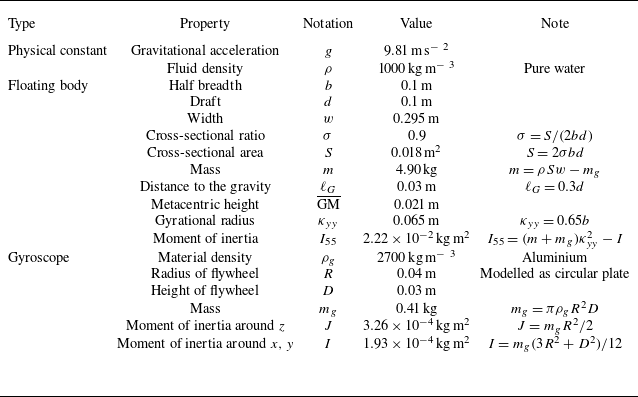


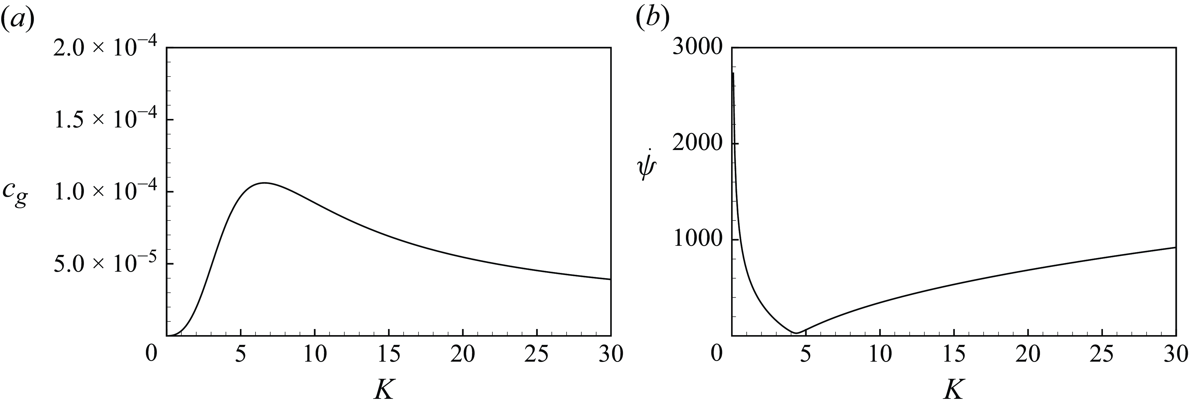


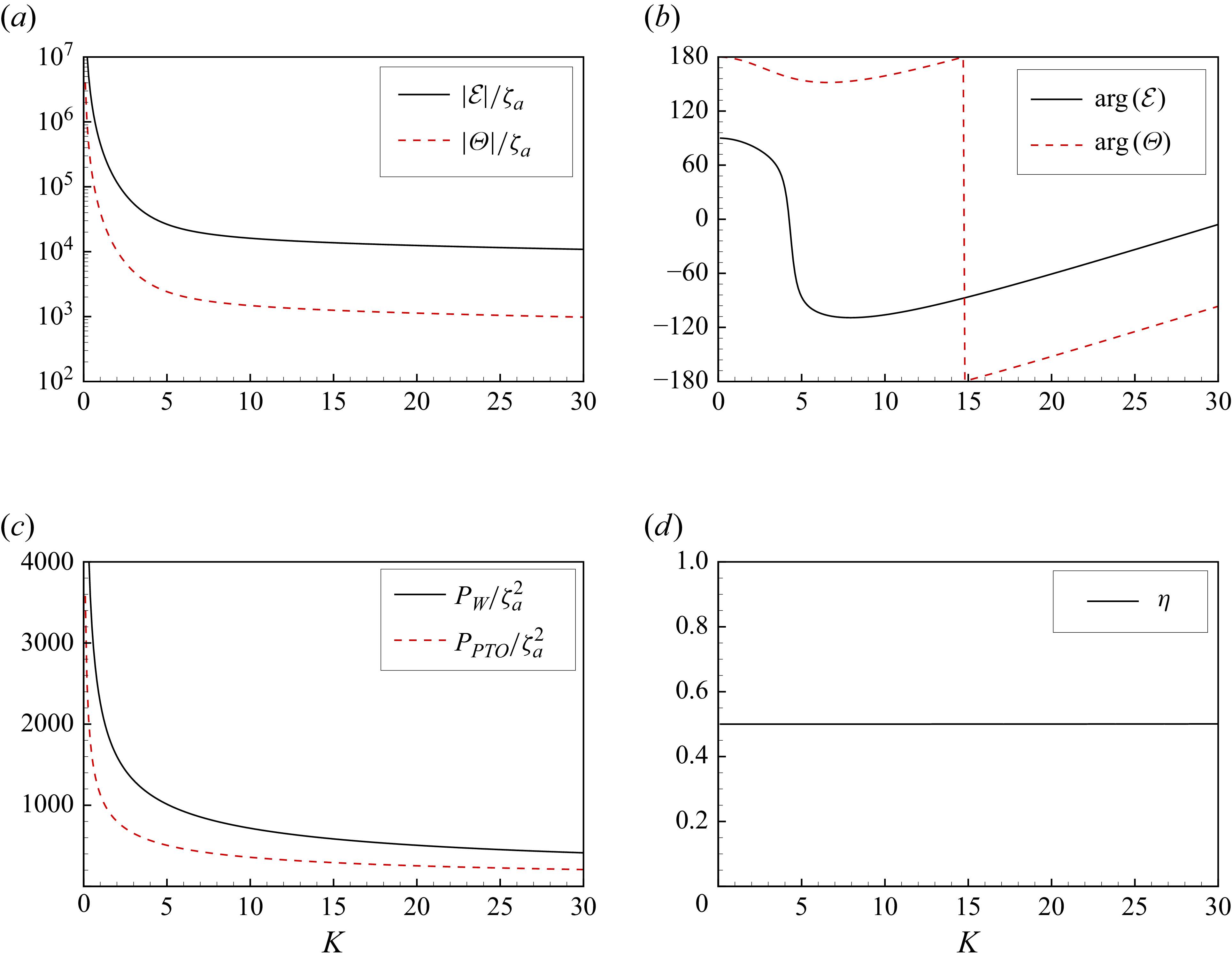


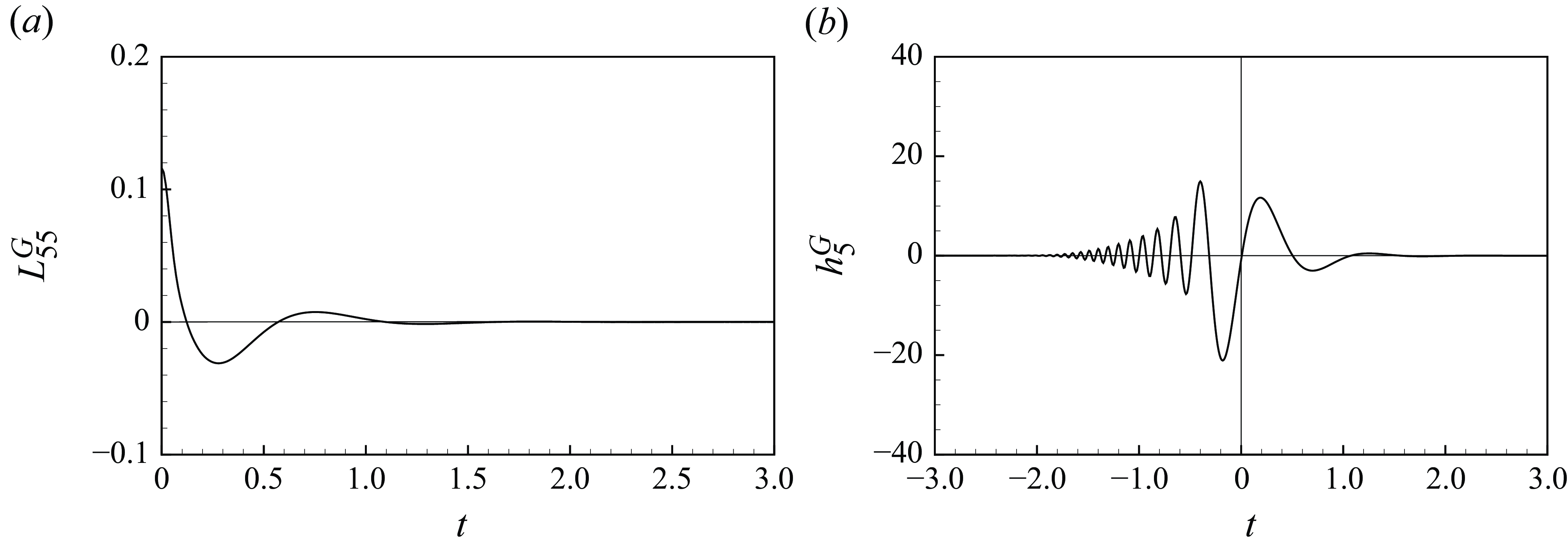


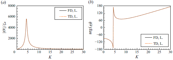


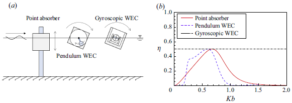


 Open access