


1. Introduction
Understanding the physics linking water surface behaviour and underlying hydrodynamics is important for numerous environmental and engineering applications such as gas and heat transfer across a free surface boundary and non-contact flow monitoring. The interaction between a water surface and the turbulent flow underneath is complex, involving a number of processes. On the one hand, it has been widely acknowledged that the water surface of a turbulent channel flow over a rough bed deforms in response to non-uniform and unsteady momentum transport and resonance processes within the flow beneath the surface. On the other hand, large-scale vertical fluid motions are flattened and redistributed to streamwise and lateral motions when approaching the water surface (Guo & Shen Reference Guo and Shen2010).
As discussed by Brocchini & Peregrine (Reference Brocchini and Peregrine2001), the interaction between a turbulent flow and the water surface is known to produce a variety of water surface deformation patterns, which can be the direct local manifestation of near-surface coherent turbulent structures (e.g. vortex dimples, scars, boils) or the result of resonances or instabilities, which selectively amplify certain periodic modes (e.g. gravity waves). The boundaries between these two processes are not well defined. For instance, Teixeira & Belcher (Reference Teixeira and Belcher2006) showed numerically that turbulent pressure fluctuations can excite quasi-periodic forced deformations, which can transition to gravity waves when the forcing ceases or alternatively decays. Gravity waves are known to occur at the margins of turbulent boils (Longuet-Higgins Reference Longuet-Higgins1996), but water surface waves can also distort and modify turbulence (e.g. Teixeira & Belcher Reference Teixeira and Belcher2002; Guo & Shen Reference Guo and Shen2013).
Experimental studies of turbulent open channel flows have shown the simultaneous presence of gravity waves and other non-dispersive surface deformations that propagate at a speed close to the speed of the flow near the water surface (Savelsberg & van de Water Reference Savelsberg and van de Water2009; Dolcetti et al. Reference Dolcetti, Horoshenkov, Krynkin and Tait2016; Dolcetti & García Nava Reference Dolcetti and García Nava2019). The presence of multiple types of surface deformations, including dispersive waves with different velocity and direction of propagation, the possibility of interactions among different scales, and the local modification of turbulent structures near the water surface, may all be reasons for the difficulty in providing a clear description of the interaction between turbulence and water surface deformations for all flow conditions.
Considering the complexity and expense of eddy-resolving numerical simulations of open-channel flows, the vast majority of these have employed a prescribed water level together with a free-slip boundary condition (i.e. rigid lid approximation) to represent the water surface. The surface-elevation-gradient terms in the momentum equations for free-surface flows are replaced by pressure gradients in this approximation, so the dynamic effects of water surface variations are properly accounted for. Such an approximation has been proved valid by several studies (Kara et al. Reference Kara, Stoesser, Sturm and Mulahasan2015b; McSherry, Chua & Stoesser Reference McSherry, Chua and Stoesser2017) and to be applicable to open channel flows with low Froude numbers and generally very small surface deviations. These studies have provided significant insights into open-channel flows in which wall-generated turbulence dominate the turbulence statistics. Only few eddy-resolving numerical studies of open-channel flow focused on deformable free surfaces. Shen & Yue (Reference Shen and Yue2001) used both direct numerical simulation (DNS) and large-eddy simulation (LES) to investigate the interactions between a turbulent shear flow and free surface at low Froude numbers. Comparisons between DNS and LES show that closer to the free surface, less energy is transferred from grid scale to subgrid-scale, which is associated with vertical motions approaching zero at the water surface and thus the highly anisotropic nature of the flow at the water surface. Shi, Thomas & Williams (Reference Shi, Thomas and Williams2000) performed LES of open channel flow at Froude ( $Fr$) and Reynolds ( $Re$) numbers of ${Fr}=0.66$ and ${Re}=20\,800$, showing that the mean turbulence kinetic energy increases when the flow approaches the water surface. Energy from vertical velocity components is mostly redistributed to the spanwise component.
Apart from open-channel flows over smooth beds, fewer numerical or experimental studies focused on the link between water surface deformation and the flow structures generated by bed features. Xie, Lin & Falconer (Reference Xie, Lin and Falconer2014) performed open-channel flow simulations over a two-dimensional (2-D) dune using LES. The predicted water surface showed the steepest slope above the recirculation region, where substantial flow deceleration takes place and where the minimum water surface fluctuations were observed. McSherry, Stoesser & Chua (Reference McSherry, Stoesser and Chua2018) performed LES of free-surface flow over square bars at varying spacings and relative submergences. Their results exhibited visible standing waves in the large bar-spacing cases, whilst the water surface hardly deformed in the small-spacing cases. In their experiments, Mandel et al. (Reference Mandel, Rosenzweig, Chung, Ouellette and Koseff2017, Reference Mandel, Gakhar, Chung, Rosenzweig and Koseff2019) measured the surface deformations induced by a submerged canopy, inferring a link between surface slope distributions and the spanwise vortices generated at the shear layer, while Gakhar, Koseff & Ouellette (Reference Gakhar, Koseff and Ouellette2020) demonstrated the diversity of surface patterns originating above different types of bottom features, such as canopy, dunes or spheres.
Although the mechanism for boils (i.e. surface-renewal eddies) produced by flow separation downstream of a bedform has been demonstrated by previous studies (Jackson Reference Jackson1976; Muraro et al. Reference Muraro, Dolcetti, Nichols, Tait and Horoshenkov2021), to the authors’ best knowledge, there are few numerical studies focused on the interrelation between surface excitation and the form-induced large sub-surface turbulence scales. Free-surface flows experiencing a sudden geometric expansion remain of fundamental research interest due to the complex hydrodynamics featuring flow separation and reattachment processes. Similar open channel flows to a backward-facing step flow are ubiquitous in nature, for example, flows over dunes or over natural beds with depth-scale geomorphological features such as in step-pool systems or over engineered structures such as broad-crested weirs. Extensive experimental and numerical research has been conducted to examine different aspects of backward-facing step flows, such as skin-friction (Jovic & Driver Reference Jovic and Driver1995), expansion ratio (Adams & Johnston Reference Adams and Johnston1988; Ötügen Reference Ötügen1991), Reynolds number effects (Friedrich & Arnal Reference Friedrich and Arnal1990; Schram, Rambaud & Riethmuller Reference Schram, Rambaud and Riethmuller2004; Nadge & Govardhan Reference Nadge and Govardhan2014), as well as vortex shedding and shear layer flapping (Eaton Reference Eaton1980; Hu, Wang & Fu Reference Hu, Wang and Fu2016). Nevertheless, understanding of the interaction between step-generated flow structures and free-surface dynamics is currently limited. In addition to the evolution of turbulent structures, studies have demonstrated that even a small variation of free-surface elevation can noticeably change the pressure level and distribution within a backward-facing step flow (Nakagawa & Nezu Reference Nakagawa and Nezu1987). Therefore, an explicit numerical model of backward-facing step flow with free-surface capturing is needed to better understand the processes of how the shear layer turbulence is modulated in response to the dynamics of the water surface.
This paper reports on large-eddy simulations of subcritical open-channel flow over a backward-facing step, a 2-D geometry which creates a complex three-dimensional (3-D) unsteady flow that contains significant turbulence-generated structures. The objectives of the study are to visualize and quantify how step-generated flow separation and reattachment (and the turbulence structures evolving from that motion) contribute to deformation of the water surface, to classify the water surface deformation and to provide insights into the physical mechanisms causing it and any interactions with the underlying flow.
2. Methodology
2.1. Large-eddy simulation
The open-source large-eddy simulation code Hydro3D is employed to simulate open-channel flow over a backward-facing step. The code has been validated and applied to a number of open-channel flow applications, e.g. Nikora et al. (Reference Nikora, Stoesser, Cameron, Stewart, Papadopoulos, Ouro, McSherry, Zampiron, Marusic and Falconer2019), Stoesser, McSherry & Fraga (Reference Stoesser, McSherry and Fraga2015), Ouro & Stoesser (Reference Ouro and Stoesser2019) and Chua et al. (Reference Chua, Fraga, Stoesser, Hong and Sturm2019). The code solves the spatially filtered Navier–Stokes equations in an Eulerian framework:
 \begin{gather} \boldsymbol{\nabla}\boldsymbol{\cdot}\boldsymbol{u}=0, \end{gather}
 \begin{gather} \frac{\partial\boldsymbol{u}}{\partial{t}} =-\frac{1}{\rho}\boldsymbol{\nabla}{p}-\boldsymbol{u} \boldsymbol{\cdot}\boldsymbol{\nabla}\boldsymbol{u} +\nu\nabla^{2}\boldsymbol{u}-\boldsymbol{\nabla}\tau+\boldsymbol{f}+\boldsymbol{g}, \end{gather}
where  $\boldsymbol {u}$ denotes the filtered resolved velocity field, ${p}$ denotes the pressure, $\nu$ is the kinematic viscosity, $\boldsymbol {f}$ represents the volume force from the immersed boundary method used to represent the effect of the step and $\boldsymbol {g}$ is the gravitational acceleration. The sub-grid scale stress tensor, $\tau$, results from unresolved small-scale fluctuations, and is approximated by the wall-adapting local eddy-viscosity (WALE) model (Nicoud & Ducros Reference Nicoud and Ducros1999) for the case presented in this paper. Hydro3D is based on finite differences with staggered storage of 3-D velocity components and central storage of pressure on Cartesian grids.
The governing equations (2.1) and (2.2) are advanced in time by the fractional-step method (Chorin Reference Chorin1968). In the predictor step, convection and diffusion terms are solved via an explicit three-step Runge–Kutta predictor. Fourth- and second-order central difference schemes are used to approximate convective and diffusive terms, respectively. In the corrector step, the pressure and a divergence-free velocity field are obtained by solving the Poisson equation via a multigrid iteration scheme (Cevheri, McSherry & Stoesser Reference Cevheri, McSherry and Stoesser2016).
The free surface is captured using the level set method (LSM) proposed by Osher & Sethian (Reference Osher and Sethian1988). The LSM introduces a level set signed distance function  $\phi$:
 \begin{gather} \phi(\boldsymbol{x},t)<0 \quad {\rm if} \ \boldsymbol{x}\in\varOmega_{gas}, \end{gather}
 \begin{gather} \phi(\boldsymbol{x},t)=0 \quad {\rm if} \ \boldsymbol{x}\in\varGamma, \end{gather}
 \begin{gather} \phi(\boldsymbol{x},t)>0 \quad {\rm if} \ \boldsymbol{x}\in\varOmega_{liquid}, \end{gather}
where  $\varOmega _{gas}$ and $\varOmega _{liquid}$ represent air or fluid phases, respectively, and $\varGamma$ denotes the interface. The movement of the interface is expressed in a pure advection equation of the following form:
 \begin{equation} \frac{\partial{\phi}}{\partial{t}}+\boldsymbol{u}\boldsymbol{\cdot}\boldsymbol{\nabla}\phi=0. \end{equation}
A multi-phase transition zone is accomplished via a Heaviside function to handle the numerical instabilities resulting from the density and viscosity discontinuities across the interface. In addition, the re-initialization technique proposed by Sussman, Smereka & Osher (Reference Sussman, Smereka and Osher1994) is employed to maintain  $|\boldsymbol {\nabla }\phi |=1$ as time proceeds. A fifth-order weighted essentially non-oscillatory (WENO) scheme is chosen to discretize (2.4) to ensure stability and minimize numerical dissipation for this pure advection equation. The validity of the LSM in the current code has been shown previously for various applications including open-channel flow over cubes and square bars (McSherry et al. Reference McSherry, Chua and Stoesser2017, Reference McSherry, Stoesser and Chua2018), and for open-channel flows past bridge abutments (Kara et al. Reference Kara, Stoesser, Sturm and Mulahasan2015b; Kara, Stoesser & Sturm Reference Kara, Stoesser and Sturm2015a).
Spatial-decomposition-based standard message passing interface (MPI) is used to accomplish the communications between pre-allocated computational subdomains. Such a technique is necessary to manage and balance the computational load to provide sufficiently fine grids in LES (Ouro et al. Reference Ouro, Fraga, Lopez-Novoa and Stoesser2019).
Figure 1 shows the flow domain for the large-eddy simulation. In the simulation, the downstream water depth is three times the step height  ${h}$, and the upstream water depth is $2h$ leading to an expansion ratio $Er=h_2/h_1=1.5$, where $h_2/h_1$ is the downstream-depth-to-upstream-depth ratio. The flow has a moderate Reynolds number (based on step height and upstream mean velocity) of $Re=4380$ and the Froude number (based on downstream mean velocity and water depth) is $Fr=0.19$. The computational domain consists of a streamwise length of $L_x=30h$, which includes a length $8h$ upstream to reduce any potential inlet artefacts, and a section of $22h$ downstream of the step to ensure full flow recovery. The spanwise width of the domain is $L_y=9h$, which is confirmed by several preliminary tests to be wide enough to not lock-in spanwise vortices or surface waves as a result of a lateral periodic boundary condition. The wall-normal height of the domain is $L_z=4h$ which includes the air phase above the water. No-slip boundary conditions are applied at the channel bed and step surfaces. A realistic inlet boundary is achieved by providing instantaneous velocity data from a fully developed precursor channel flow with equivalent grid and temporal resolution at the domain inlet. The precursor simulation is validated with data of the direct numerical simulation of turbulent channel flow by Moser, Kim & Mansour (Reference Moser, Kim and Mansour1999). For brevity, this is not shown here but can be found in Cevheri et al. (Reference Cevheri, McSherry and Stoesser2016). Aider, Danet & Lesieur (Reference Aider, Danet and Lesieur2007) examined different inlet conditions for backward-facing step flow. One condition is to prescribe a mean turbulent profile perturbed by white noise while the second condition is the same as the one used in this study. Their results demonstrate the adequacy of this treatment and the necessity of imposing realistic time-dependent inlet conditions.
Sketch of the computational domain.

The computational domain is discretized using a uniform grid of  $480 \times 144 \times 128$ ( $= 8.8 \times 10^6$) points in the streamwise, spanwise and wall-normal directions, and the grid has an aspect ratio of $2:2:1$. The maximum near-wall grid spacing, $\Delta z^+_{max}$, which is found in the region of the fully recovered boundary layer downstream of the step, is approximately 3.5. The time step in LES is fixed at $0.00243h/U_{max}$, where $U_{max}$ is the maximum streamwise velocity observed at location $x/h=-1$ and $z/h=+2.8$. Collecting of instantaneous flow quantities starts after $1123h/U_{max}$ has elapsed (i.e. 25 flow through periods), and continues for a duration of $476h/U_{max}$ (i.e. more than 10 further flow through periods) to ensure that the turbulence statistics are well converged. The data set of instantaneous quantities for subsequent analysis is extracted from $x/h=-1$ to $x/h=20$, with spatial resolution of $\Delta x = 0.125h$, $\Delta y = 0.125h$, $\Delta z = 0.0625h$ and at a time interval $\Delta t = 0.06075h/U_{max}$. Only simulation results of the water phase are presented in the following sections.
2.2. Water surface dynamics
The interaction between the turbulent flow and the water surface involves a multitude of scales and multiple nonlinear processes that can be difficult to identify. The approach followed here is to decompose the water surface deformation (with respect to the time-averaged profile) into various types of waves according to their dispersion or velocity of propagation.
Surface deformations induced locally by rising turbulent eddies are believed to travel at the same speed as the forcing, following the eddy that advects downstream. Assuming that only turbulent structures close to the water surface are able to cause a significant deformation, forced deformations should propagate approximately at the surface velocity  $U_0 = U(z=d)$. Applying a Fourier decomposition to the surface fluctuations, the non-dimensional frequency of the terms with wavenumber vector ${\boldsymbol k}$ (where $|{\boldsymbol k}| = k = 2{\rm \pi} /\lambda$ and $\lambda$ is the wavelength) would be
 \begin{equation} \frac{h}{U_{max}} \varOmega_{F}({\boldsymbol k}) = ({\boldsymbol k}h)\boldsymbol{\cdot}\frac{ {\boldsymbol U}_0}{ U_{max}}, \end{equation}
as demonstrated experimentally by Savelsberg & van de Water (Reference Savelsberg and van de Water2009) and Dolcetti et al. (Reference Dolcetti, Horoshenkov, Krynkin and Tait2016), where  $f = \varOmega _{F}({\boldsymbol k})/2{\rm \pi}$ is a frequency in Hz.
Gravity waves propagate relative to the flow velocity, potentially in all directions. The calculation of the speed of gravity waves in a vertically sheared viscous flow with a variation in the channel cross-section is not trivial, and is limited to circumstances of gradually varying water depths (e.g. Li & Ellingsen Reference Li and Ellingsen2019). For the purposes of the interpretation of LES results in this study, it is deemed sufficient to use gravity wave equations derived for an inviscid and irrotational flow. Accordingly, the speed of propagation of a wave relative to the flow velocity (also called the intrinsic wave speed) is
 \begin{equation} c_i = \sqrt{\frac{g}{k}\tanh(kd)}. \end{equation}
In a fixed frame of reference, the frequency of water surface fluctuations due to a gravity wave with wavenumber vector  ${\boldsymbol k}$ that propagates over a flow with average surface velocity ${\boldsymbol U}_0$ is $f = \varOmega _{\pm }({\boldsymbol k})/2{\rm \pi}$, where
 \begin{equation} \frac{h}{U_{max}} \varOmega_{{\pm}}({\boldsymbol k}) = ({\boldsymbol k}h)\boldsymbol{\cdot}\frac{ {\boldsymbol U}_0}{ U_{max}} \pm kh \frac{c_i}{U_{max}} = kh\left[ \frac{{\boldsymbol k}\boldsymbol{\cdot}{\boldsymbol U}_0}{k U_{max}} \pm \frac{1}{{\sf F}_{max}}\sqrt{\frac{d}{h} \frac{\tanh(kd)}{kd}}\right], \end{equation}
where  ${\sf F}_{max} = U_{max}/\sqrt {gh}$ (
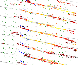
 ${\sf F}_{max} = 0.5486$ in this work) is the maximum Froude number based on the maximum average flow velocity and the step height. Equations (2.5) and 2.7 are represented in figure 2 in grey. The two signs of (2.7) identify two types of gravity waves, which are denoted GW $-$ and GW $+$, respectively. GW $+$ waves can also be separated into two groups: GW $+$d waves with a positive streamwise wavenumber component $k_x>0$, which propagate downstream; and GW $+$u waves with $k_x<0$, which propagate upstream.
Decomposition of the frequency-wavenumber spectrum of the water surface fluctuation. The grey lines represent the dispersion relation of gravity waves and of forced water surface deformations. The dashed black lines identify the boundaries of the different types of waves.

The contribution of each type of water surface deformation can be identified by filtering the water surface signal in the frequency-wavenumber space. The filtering is performed by means of an inverse Fourier transform in space and in time, applied to portions of the complex surface spectrum.
The following types of surface deformations are identified:
(i) low-frequency fluctuations, including all terms with
(2.8) \begin{equation} f h / U_{max} < 0.051; \end{equation}
(ii) forced surface deformations, including all terms with
(2.9)\begin{equation} (\varOmega_-(k) + \varOmega_F(k))/4{\rm \pi} < f < (\varOmega_+(k) + \varOmega_F(k))/4{\rm \pi}; \end{equation}(iii) GW
$-$ gravity waves, with
(2.10)\begin{equation} \varOmega_-(k)/2{\rm \pi} + (\varOmega_-(k) - \varOmega_F(k))/4{\rm \pi} < f < (\varOmega_-(k) + \varOmega_F(k))/4{\rm \pi}; \end{equation}(iv) GW
$+u$ gravity waves, with
(2.11)\begin{equation} (\varOmega_+(k) + \varOmega_F(k))/4{\rm \pi} < f < \varOmega_+(k)/2{\rm \pi} + (\varOmega_+(k) - \varOmega_F(k))/4{\rm \pi} ,\quad k_xh<0; \end{equation}(v) GW
$+d$ gravity waves, with
(2.12)\begin{equation} (\varOmega_+(k) + \varOmega_F(k))/4{\rm \pi} < f < \varOmega_+(k)/2{\rm \pi} + (\varOmega_+(k) - \varOmega_F(k))/4{\rm \pi},\quad k_xh>0. \end{equation}


The corresponding areas of the streamwise frequency-wavenumber spectra are displayed in figure 2.
The non-dimensionalized group velocity of gravity waves (i.e. the velocity of the ‘envelope’, or of a packet of waves) is
 \begin{equation} \frac{\boldsymbol c_g}{U_{max}} = \frac{ \boldsymbol{\nabla}_{\boldsymbol k}\varOmega_{{\pm}}}{U_{max}} = \frac{{\boldsymbol U_0}(x)}{U_{max}} \pm \frac{1}{2 {\sf F}_{max}}\sqrt{\frac{d}{h}\frac{\tanh(kd)}{kd}}\left[1 + \frac{2kd}{\sinh(2kd)}\right]\frac{\boldsymbol k}{k}. \end{equation}
For  ${\boldsymbol k} \parallel {\boldsymbol U_0}$, the condition $c_g = 0$ corresponds to a relative maximum of $\varOmega _\pm (k_x)$, which can be seen for $k_x<0$ in figure 2. It indicates a group that is locked in space. In the short waves limit $kd \gg 1$, this is satisfied by a wave with wavenumber $k_g$, equal to
 \begin{equation} k_gh \approx \frac{1}{4 {\sf F}_{max}^2} \frac{U_{max}^2}{U^2_{0}}. \end{equation}
A group of waves with  $c_g = 0$ remains fixed at a certain location, however, the crests of each wave within the group keep propagating, with the frequency
 \begin{equation} \frac{f_g h}{U_{max}} = \frac{h}{U_{max}}\frac{|\varOmega_-(k_gh)|}{2{\rm \pi}} \approx \frac{1}{8{\rm \pi} {\sf F}_{max}^2} \frac{U_{max}}{U_{0}}, \end{equation}
which is inversely proportional to the local value of the surface velocity  $U_0$.
Stationary waves, however, satisfy the condition  $\varOmega _\pm (\boldsymbol k)=0$. Considering only waves with the front perpendicular to the step, their wavenumber $k_s$ in the short waves limit is
 \begin{equation} k_sh \approx \frac{1}{{\sf F}_{max}^2} \frac{U_{max}^2}{U^2_{0}} = 4k_gh. \end{equation}
 Surface tension effects are not accounted for in the simulations. These effects are expected to become significant at Bond numbers  ${\sf B}< 1$, where ${\sf B} = \rho g / k^2 \gamma$, $\rho$ is the water density, $g$ is the acceleration due to gravity and $\gamma$ is the surface tension coefficient, i.e. at wavenumbers $k > 367\,{\rm rad}\,{\rm m}^{-1}$ ( $kh > 7.3$). Most surface features observed in this study have a wavenumber smaller than $kh = 3$ ( ${\sf B} = 6$), with the dominant waves with zero-group velocity having $k_gh \leq 1.8$ ( ${\sf B} \geq 17$). These values suggest that the inclusion of surface tension effects would not significantly modify the simulation results used to investigate the behaviour of the water surface in this study.
2.3. Validation of the LES
The large-eddy simulation method is validated using laboratory data from Nakagawa & Nezu (Reference Nakagawa and Nezu1987) to confirm the suitability of the selected discretization schemes, the mesh size, subgrid-scale model as well as boundary conditions. Case ST1 of Nakagawa & Nezu (Reference Nakagawa and Nezu1987) is selected for validation of the turbulence statistics and of the time-averaged water surface elevation. In the ST1 experiment, a  $h = 2$ cm backward-facing step was placed $6.8$ m downstream of an $8$ m long, $30$ cm wide rectangular channel followed by a long outlet channel downstream of the step. Velocity profiles were measured at several downstream locations along the channel centreline using a laser Doppler anemometry (LDA) system and the water surface elevation was measured by a moving manual point gauge.
Profiles of LES-computed time- and spanwise-averaged streamwise velocity, streamwise and wall-normal velocity fluctuations, as well as the Reynolds shear stresses at selected centreline locations are plotted in figure 3. Overall, the LES results show convincing agreement with measured data (open circles) for time-averaged streamwise velocities at a range of locations downstream of the step. Flow acceleration above and reverse flow inside the recirculation zone is predicted particularly accurately, as seen from the streamwise velocity distributions, and so is the recovering boundary layer downstream of the time-averaged reattachment point. Long dashed lines in figure 3 denote the time- and spanwise-averaged dividing streamline  $(i.e. \int _{0}^{h_2} \langle u \rangle \,{\rm d}z=0)$. The reattachment length is therefore estimated to be $6.15h$, which agrees well with the experimental data. Kuehn (Reference Kuehn1980), Nadge & Govardhan (Reference Nadge and Govardhan2014) and Nakagawa & Nezu (Reference Nakagawa and Nezu1987) have demonstrated that the reattachment length increases with a decrease in relative submergence (downstream-depth-to-step-height ratio, $h_2/h$). In addition, De Brederode (Reference De Brederode1972) and Nadge & Govardhan (Reference Nadge and Govardhan2014) suggested that the channel-width-to-step-height ratio, ${A_{r}}$, has an impact on the reattachment length. It is noteworthy here that the ${A_{r}}$ is 15 in the experiment and infinite in the LES, inferring that the reattachment length observed in the experiment or the simulated value in LES is affected by the secondary structures generated by the sidewalls (De Brederode Reference De Brederode1972). Jovic & Driver (Reference Jovic and Driver1995) demonstrated that the reattachment length increases with an increasing step height Reynolds number while keeping the boundary-layer-thickness-to-step-height ratio unchanged, where the ${A_{r}}$ is sufficiently large in all their experiments to ensure essentially two-dimensionality in the separated region. Furthermore, as the upstream boundary layer is fully turbulent in the current case, the reattachment length is not considered to be affected by the upstream boundary layer thickness (Adams & Johnston Reference Adams and Johnston1988). Figure 3 presents profiles of streamwise and wall-normal velocity fluctuations and Reynolds shear stresses normalized by $U_{max}$ at various locations downstream of the step. Overall, the agreement between the LES and experimental observations regarding the normal stresses is quite satisfying (except for $\langle u \rangle '$ very close to the water surface). However, the LES results overpredict the Reynolds shear stress from $x/h = 10$ onwards. These discrepancies are most probably due to the presence of secondary currents induced by the sidewalls in the experiment. As described by Nezu & Nakagawa (Reference Nezu and Nakagawa2017) and quantified by Nikora et al. (Reference Nikora, Stoesser, Cameron, Stewart, Papadopoulos, Ouro, McSherry, Zampiron, Marusic and Falconer2019), secondary currents can contribute significantly to streamwise momentum, thereby reducing the contribution of the turbulent Reynolds shear stress to the total stress. Secondary currents are non-negligible in narrow open channel flows where the channel-width-to-water-depth ratio is less than 6. The channel-width-to-downstream-water-depth ratio in the experiment is approximately 5, whereas the ratio is infinity in LES due to the use of periodic boundary conditions in the spanwise direction. The use of a periodic boundary condition in the spanwise direction ensures that water surface deformations are caused only by the step. To support the aforementioned statement that the Reynolds stress discrepancies are primarily due to the sidewall effect, an additional backward-facing step flow simulation is performed. The results of this LES are also plotted in figure 3(d) together with the experimental data of the wind tunnel experiment conducted by Jovic & Driver (Reference Jovic and Driver1995). In the experiment of Jovic & Driver (Reference Jovic and Driver1995), the channel-width-to-step-height ratio was twice that of the experiment of Nakagawa & Nezu (Reference Nakagawa and Nezu1987), hence secondary currents are expected to be less significant. As can be seen, the LES indeed matches the measured Reynolds shear stress profiles quite accurately. Regardless of the aspect ratio, the turbulent fluctuations and shear stresses are markedly higher above the recirculation zone, e.g. at $x = 1h$ and $z \approx 1h$, and display a distinct maximum around the dividing streamline. The peaks in the profiles decay only slowly in the downstream direction and indicate significant and persistent shear-layer turbulence.
Profiles of the time- and spanwise-averaged streamwise velocity, streamwise and wall-normal velocity fluctuations, as well as Reynolds shear stresses at various locations along the streamwise direction. Open symbols, experimental data from Nakagawa & Nezu (Reference Nakagawa and Nezu1987) (circles) and Jovic & Driver (Reference Jovic and Driver1995) (triangles); solid lines, LES data corresponding to the experiment of Nakagawa & Nezu (Reference Nakagawa and Nezu1987); dashed lines, LES time- and spanwise-averaged dividing streamline; dash–dotted lines, LES corresponding to the experiment of Jovic & Driver (Reference Jovic and Driver1995).

Figure 4 presents computed and measured profiles of the time-averaged water surface along the streamwise direction as well as the theoretical profile proposed by Nakagawa & Nezu (Reference Nakagawa and Nezu1987). To the best of the authors’ knowledge, the study of Nakagawa & Nezu (Reference Nakagawa and Nezu1987) is the only experimental open-channel backward-facing step flow study in which velocity data and the surface elevation were measured. The measured streamwise increase in time-averaged water depth from upstream to downstream of the step is modest at approximately 1 mm. Figure 4 illustrates that the LES successfully captures the overall increase in time-averaged water depth in the downstream direction. The LES-predicted water surface profile matches with the theoretical profile quite well; however, the match just downstream of the step is not as good. Manual point gauges do not provide a time series of the water surface elevation, the estimation of the time-averaged elevation by Nakagawa & Nezu (Reference Nakagawa and Nezu1987) could have been affected by observational bias that scales with the water waves’ amplitudes, and this may explain the discrepancies observed in the time-averaged water levels just downstream of the backward step. This argument is supported by the contemporaneous comments of Nakagawa & Nezu (Reference Nakagawa and Nezu1987) stating that ‘Although the accuracy of the point gauge was 1/20 mm it was very difficult to accurately measure the elevation of the free surface because of the fluctuations of water waves.’
Time- and spanwise-averaged water surface elevation as a function of streamwise distance from the step. The theoretical line (dotted) is derived from the energy gradient as demonstrated by Nakagawa & Nezu (Reference Nakagawa and Nezu1987).

3. Water surface deformation characteristics
Figure 5 shows the frequency-wavenumber power spectral density (PSD) of the water surface fluctuations downstream of the step. The spectrum is calculated for intervals of  $121.5 h/U_{max}$ duration, with a Hann window in time and with 50 % overlap, resulting in six degrees of freedom. The quantities shown in figure 5(a,b) are plotted for the two cross-sections with $k_y=0$ and $k_x=0$, corresponding to spectra in the streamwise and in the spanwise direction, respectively. The large values of the spectra at $k_x = k_y = 0$ in both figures are due to the definition of surface fluctuations, which is based on removal of the temporal average at each location (rather than of the spatial average at each time step), and to the non-periodicity of the water surface elevation in the streamwise direction.


The dashed lines represent the dispersion relation of gravity waves, (2.7), and are calculated based on the streamwise averaged surface velocity  $\langle {U}_0 \rangle = 0.823 U_{max}$. Gravity waves propagating in all directions are observed. The four types of waves (GW $-$, GW $+$u, GW $+$d and forced deformations) can be identified by comparison of figure 5(a) with figure 2. Both lines in figure 5(b) correspond to GW $+$ waves which are propagating along the spanwise direction with $k_x=0$. Another large peak of the streamwise spectrum in figure 5(a) is found along a horizontal line with frequency $fh/U_{max} \approx 0.05$, with broad wavenumber content.
Figure 6 shows how the spanwise-averaged frequency PSD of the surface fluctuations calculated in time vary along the streamwise direction. The spectral density distributions are characterized by a broadband background and three peaks. The background decreases rapidly with frequency and is almost independent of the location. The first two peaks occur at a frequency of  $f h /U_{max} \approx 0.05$ and at its first harmonic, $f h /U_{max} = 0.1$. The peaks disappear briefly at $x/h\approx 4$ and at $x/h\approx 10$. The frequency of the third peak, instead, increases along $x$ proportionally to $1/U_0(x)$, matching well with the frequency $f_g h /U_{max}$ of the waves with a stationary wave group (dotted line in figure 6) calculated as a function of the time-averaged local surface velocity $U_0(x)$ according to (2.15). The apparent deviation from (2.15) observed at $x/h \geq 11$ can be explained considering the range of variability of $U_0$ in time.
Streamwise variation of the frequency PSD spectrum of the water surface elevation (in dB). Dashed line,  $f h /U_{max} =0.05$; dash–dotted line, $f h /U_{max} =0.1$; dotted line, gravity waves with zero group-velocity, (2.15).

The water surface fluctuations are subsequently decomposed into the types of waves proposed in § 2.2 by means of an inverse Fourier transform applied to portions of the complex frequency-wavenumber spectrum identified according to figure 2. The original water surface deformation together with its decomposed constituents at an arbitrary instant in time are presented in figure 7. In accordance with the frequency spectra shown in figure 6, low-frequency fluctuations (figure 7b) are dominant. They correspond to quasi-one-dimensional large-scale depth variations along the streamwise direction, with a strong periodicity in time. Other constituents are smaller in amplitude, therefore they are shown with a different scale in figure 7(c–f). All constituents exhibit alternating bands aligned along the transverse direction, where the water surface appears rougher and dominated by smaller scales of deformation (e.g. at  $6 < x/h < 9$ and at $15 < x/h < 18$ in figure 7), separated by relatively smooth regions ( $9 < x/h < 14$ in figure 7). The rougher bands include the instantaneous maxima of the modulus of the water surface slope in the streamwise direction, $|\partial \zeta '/\partial x|$, indicated by arrows. The upstream gravity-waves (GW $-$, figure 7d and GW $+$u, figure 7e) appear to be mostly one-dimensional, and dominated by waves the crests of which are perpendicular to the flow. GW $+$d (figure 7f) and forced surface deformations (figure 7e) appear more isotropic. The forced deformations include small approximately round depressions that also tend to align in bands but are stronger further downstream of the step.
Decomposed instantaneous fluctuation of the water surface relative to the time-averaged surface shape at an instant in time, normalized by  $h$: (a) unfiltered water surface elevation; (b) low-frequency surface fluctuations; (c) forced surface fluctuations; (d) GW $-$ gravity waves; (e) GW $+$u gravity waves; (f) GW $+$d gravity waves. Arrows indicate the spanwise-median streamwise position of the instantaneous points of maximum $|\partial \zeta '/\partial x|$.

The spatial spectra of the surface fluctuations are evaluated by means of a Morlet wavelet transform (Grossmann & Morlet Reference Grossmann and Morlet1984). The transform is applied in space, along the streamwise direction, to identify the characteristic spatial scales, which can be linked directly to the wavelength, allowing for a direct comparison with the Fourier spectrum (Meyers, Kelly & O'Brien Reference Meyers, Kelly and O'Brien1993). The approach has been used by various authors for the analysis of surface wave data (e.g. Donelan, Drennan & Magnusson Reference Donelan, Drennan and Magnusson1996; Massel Reference Massel2001; Dolcetti & García Nava Reference Dolcetti and García Nava2019; Gakhar, Koseff & Ouellette Reference Gakhar, Koseff and Ouellette2022). Figure 8 presents the time- and spanwise-averaged absolute wavelet spectra of each term of the decomposed surface fluctuations. Low-frequency fluctuations (figure 8c) show a predominance of long waves with  $kh\sim 1$, as well as a peak at the wavenumber of the stationary waves, $k_sh$ (2.16, dotted line in figure 8). The other terms of the surface decomposition appear to be linked to the wavenumber and frequency of the waves with $c_g=0$: $k_g$ and $f_g$ ((2.14) and (2.15)). The wavelet spectrum of GW $-$ waves (figure 8b) has a peak in the region $6 \leq x/h \leq 15$, at a wavenumber of $(1+\sqrt {2})^2 k_g h \approx 6k_g h$. The wavelet spectra of GW $+$u waves (figure 8d) and GW $+$d waves (figure 8f) are dominated by longer waves, with wavenumber $\approx k_gh$. Forced surface deformations (figure 8e) appear to be shorter and to have a peak in the region $10 \leq x/h \leq 15$, at the wavenumber $kh \approx 2k_gh$. According to (2.7) and (2.5), these wavenumbers yield the frequencies $\varOmega _-((1+\sqrt {2})^2 k_g h)/2{\rm \pi} = f_g$ (GW $-$),
$-$),  $\varOmega _+(-k_g h)/2{\rm \pi} = f_g$ (GW $+$u), $\varOmega _+(k_g h)/2{\rm \pi} = 3f_g$ (GW $+$d) and $\varOmega _F(2 k_g h)/2{\rm \pi} =2f_g$ (forced deformations).
Average spatial wavelet spectrum of the decomposed water surface fluctuation along the streamwise direction: (a) unfiltered water surface elevation; (b) GW $-$ gravity waves; (c) low-frequency surface fluctuations; (d) GW $+$u gravity waves; (e) forced surface fluctuations; (f) GW $+$d gravity waves. Solid line, $kh = k_gh$ (2.14); dashed line, $kh = 2k_gh$; dash–dotted line, $kh = (1+\sqrt {2})^2 k_gh$; dotted line, $kh = k_sh = 4k_gh$ (2.16).

Figure 9 summarizes the streamwise wavenumber and frequency coordinates of the peaks observed in the wavelet spectra of the surface deformations (figure 8). As a possible explanation for the appearance of these peaks, it is noted that GW $+$u and GW $+$d waves with wavenumber $k_g$ can form a resonant triad with a forced wave with wavenumber $2k_g$ and frequency $2f_g$. Three waves with wavenumbers ${\boldsymbol k}_1$, ${\boldsymbol k}_2$ and ${\boldsymbol k}_3$, and with frequencies $f_1$, $f_2$ and $f_3$ are said to constitute a resonant triad when ${\boldsymbol k}_1 \pm {\boldsymbol k}_2 \pm {\boldsymbol k}_3 = 0$ and $f_1 \pm f_2 \pm f_3 = 0$ (e.g. Phillips Reference Phillips1960). Here, the pair of GW $+$ waves and forced deformations satisfy
 \begin{equation} k_g+k_g-2k_g = 0, \end{equation}
and
 \begin{equation} \varOmega_+(k_gh) - \varOmega_+(-k_gh) -\varOmega_{F}(2k_gh) = 3f_g - f_g - 2f_g = 0, \end{equation}
therefore exchange of energy among these waves is possible. An interaction between two gravity waves with the same wavenumber modulus but different direction of propagation, and a shorter non-dispersive disturbance, has been described by Zakharov & Shrira (Reference Zakharov and Shrira1990), with the forced-wave replaced by a perturbation of a sheared flow at the critical layer. The same mechanism was suggested to allow a transfer of energy between stationary waves, turbulence and freely propagating gravity waves in turbulent open channel flows over rough beds (Dolcetti & García Nava Reference Dolcetti and García Nava2019), or between gravity waves and vorticity waves (Drivas & Wunsch Reference Drivas and Wunsch2016) or internal waves (Thorpe Reference Thorpe1966). Here, it is suggested that the same mechanism allows the exchange of energy between a pair of counter-propagating gravity waves and a forced surface deformation, specifically for a case where one of the gravity waves has  $c_g=0$.

Figure 10 presents the surface variance in the streamwise direction and demonstrates how each constituent of the surface decomposition contributes to the water surface deformation (figure 10a) and of its first- (figure 10c) and second-order streamwise gradient (figure 10e). The lines in figure 10(b,d,f) show the variance of each term of the decomposition normalized by the variance of the unfiltered surface fluctuations. These plots quantify the contributions of each constituent of the water surface variance along  $x$. The apparent strong effect of the normalization is due to relatively large variations of the unfiltered variance in space. Close to the step, the variance of the surface elevation fluctuations $<\zeta '^2>/h^2$ (figure 10a,b) initially decreases with $x/h$, for $x/h < 4$. Then, it has a first peak in the region between $x/h = 4$ and $x/h = 10$, which corresponds to the region where the average depth gradient is larger (see figure 4). A second peak is found at $x/h \approx 17$. The variance of $\zeta '$ is dominated by the low-frequency terms, which contribute to between 20 % and 80 % of the unfiltered variance. The second largest contribution is due to GW $+$u waves, and it is between 10 % and 50 %. The variance of $\zeta '_x$ (figure 10c), instead, has a peak at $x/h \approx 10$ and it shows a more balanced contribution from the different terms of the surface decomposition (figure 10d). Low-frequency fluctuations, GW $-$, and GW $+$u terms are larger in the region between $x/h = 3$ and $x/h = 15$, while forced fluctuations are larger between $x/h = 10$ and $x/h = 20$. As a result, GW $+$u terms are predominant (between 30 % and 50 %) for $x/h < 11$, while the contribution of forced fluctuations dominates the region further downstream. The variance of the second spatial derivative $\zeta '_{xx}$ represents the effect of the shortest scales of the water surface. Its spatial distribution (figure 10e) has a marked peak at $x/h = 13$, which is caused mostly by the contribution of forced fluctuations and GW $-$ terms (figure 10f).
Streamwise distribution of the variance of the water surface fluctuations. Each line represents a different constituent of the water surface deformation. (a,c,e) Non-dimensionalized variance. (b,d,f) Variance of the filtered surface normalized with the variance of the unfiltered surface. (a,b)  $\zeta '$; (c,d) $\zeta '_x$; (e,f) $\zeta '_{xx}$.

4. Statistics of the flow field
The average PSD of the streamwise (a–d), spanwise (e–h) and wall-normal (i–l) velocity fluctuations at selected streamwise and wall-normal locations are presented in figure 11. In many of the spectra of the streamwise and wall-normal velocity components, a peak at the frequency  $f h/U_{max} = 0.05$ is observed. This peak is followed by a power-function decay of ${\sim }f^{-5/3}$. The peak at $f h /U_{max}=0.05$ is observed at $z=h$, just downstream of the step. Inspecting the variation of the frequency spectra along the streamwise direction at each $z$-level (not shown), it is found that the peak dominates in a region with length $\approx 13h$ along $x$, which is shifted downstream as the distance from the bed increases, from $3\leq x/h \leq 16$ at $z/h=0.5$ to $5\leq x/h \leq 18$ at $z/h=2.69$. This suggests the presence of a large, energetic turbulence structure that is shed periodically at a low frequency from the step and is subsequently being advected in the streamwise direction and towards the water surface by the flow. The spectra of the spanwise velocity fluctuations do not exhibit such a distinct peak, it is rather weak, suggesting a quasi-2-D turbulence structures, owed to the quasi-2-D geometry. The spectrum of the wall-normal velocities has an additional peak at the harmonic $f h/U_{max} = 0.1$, while the spectrum of spanwise velocities has a peak at a lower frequency, $f h/U_{max} = 0.03$. In figure 11(i–l), the spectrum of the time-derivative of the water surface fluctuations, $\zeta _t$, is also plotted. Expanding the kinematic boundary condition at a distance $\varepsilon + \zeta$ below the water surface (e.g. Tsai Reference Tsai1998, (2.3)),
 \begin{equation} w \approx \zeta_t + \left( u\zeta \right)_x + \left( v\zeta \right)_y - w_z\varepsilon, \end{equation}
therefore the spectra of  $\zeta _t$ are expected to bear a similarity with those of $w$, at least within a limited range of frequencies. The energy in $\zeta _t$ decays with $\sim f^{-5/3}$ in the frequency range $0.2 < f h /U_{max} < 2$. At higher frequencies for shorter waves, the expansion of the boundary condition loses validity, the link between the spectra of the wall-normal velocity and those of the surface gradient weakens, and the PSD of $\zeta _t$ decays faster. At lower frequencies, a peak is observed at $f h/U_{max} = 0.05$, matching the frequency peak in the velocity signal and at $x/h=20$ a distinct secondary peak is found.
Spanwise-averaged PSD of the velocity fluctuations at different streamwise locations and distance from the bed: (a–d) streamwise velocity; (e–h) spanwise velocity; (i–l) wall-normal velocity. The colour scale indicates the distance from the bed  $z/h$. Each line has been shifted vertically by an amount equal to $10 \times z/h$ (in dB). The dash–dotted line is proportional to $f^{-5/3}$. The black solid line in panels (i–l) represents the frequency spectrum of the time-derivative of the water surface elevation, $\zeta _t$.

Figure 12 presents contours of the instantaneous vorticity magnitude in the centreplane at selected time steps together with the dividing streamline of the recirculation zone behind the step. The plots reveal different phases of the recirculation zone: a compact recirculation eddy ( $tU_{max}/h=61$ and $tU_{max}/h=82$), its growth and maximum extent ( $tU_{max}/h=67$ and $tU_{max}/h=88$), and its breakdown with subsequent shedding of a secondary vortex ( $tU_{max}/h = 73$ and $tU_{max}/h = 94$). This process has been reported previously by Hu et al. (Reference Hu, Wang and Fu2016). Levels of high vorticity are also found in the shear layer around the dividing streamlines (e.g. at $tU_{max}/h = 88$) and link with the shear layer's flapping motion, e.g. $tU_{max}/h = 94$. The latter appears to cause the initiation of additional elongated turbulent structures that stretch obliquely towards the water surface. These structures, easily observable from the snapshot at $tU_{max}/h = 82$, may be so-called kolk-boil vortices (Rodi, Constantinescu & Stoesser Reference Rodi, Constantinescu and Stoesser2013), or could correspond to the legs of hairpin vortices. In figure 12, they do not seem to be able to reach the water surface. Instead, isolated patches of high vorticity very close to the surface (e.g. at $x/h\approx 5$ and at $x/h\approx 14$ at $tU_{max}/h = 82$) appear to be disconnected from other high-vorticity regions and limited to a thin sub-surface layer of depth $\leq 0.5 h$.
Snapshots of the instantaneous vorticity magnitude at the centreline in spanwise direction.

Cross-sections of the frequency-wavenumber spectra of velocity fluctuations on the plane  $k_y = 0$ evaluated at selected $x$–
$x$– $y$ planes ( $z/h = 1, 2$ and $2.69$) are shown in figure 13. These are calculated as in figure 5(a), with a Hann window to reduce spectral leakage due to the non-periodicity along $x$. All spectra peak around the straight line that corresponds to the advection frequency $\varOmega _F({\boldsymbol k})$. The scatter around this line is significant, which indicates substantial velocity variations either in time or in space. Compared with the line $\varOmega _F({\boldsymbol k})$, which is based on the mean flow velocity at the surface, the gradient of the line followed by the spectra is smaller at lower depths, because of the lower mean velocity near the bed. A small portion of the spectra also lies along the expected dispersion relation of gravity waves. The effect is seen more clearly in the spectra of the streamwise and wall-normal velocity fluctuations, especially closer to the water surface (figure 13a,c), where both GW $+$u and GW $+$d can be identified but also at $z/h=2$ (figure 13d,f), at a considerable distance from the water surface level. These contributions represent a perturbation of the flow field that is distinguished from turbulence and is instead linked with the fluctuation of the water surface in accordance with an inviscid gravity wave theory. The relative amount of spectral energy directly attributable to gravity waves is quantified by integrating the frequency-wavenumber PSD of the flow velocity fluctuations within the regions identified in figure 2. Gravity waves are associated with 2 % and 6 % of the variance of the horizontal and wall-normal velocity fluctuations, respectively, at $z/h=2.69$.
Cross-sections of the frequency-wavenumber PSD of the velocity fluctuations, at different elevations. (a,d,g) Streamwise velocity; (b,e,h) spanwise velocity; (c,f,i) wall-normal velocity. (a–c)  $z/h = 2.69$; (d–f) $z/h = 2.00$; (g–i) $z/h = 1.00$. The dashed lines indicate the theoretical dispersion relation of gravity waves, (2.7). The dash–dotted line indicates the advection frequency $\varOmega _F/(2{\rm \pi} )$ based on the average surface velocity $\left \langle U_0\right \rangle$, (2.5). The colour scale is in dB.

5. Large-scale turbulence–water-surface interactions
5.1. Links between flow reattachment, large-scale structures and water surface deformation
With the aim to reveal the flow structures containing the most energy and to visualize the impact of the step-generated vortices on the water surface deformations, a set of instantaneous flow fields are reconstructed by the method of snapshot proper orthogonal decomposition (snapshot POD). The methodology of snapshot POD is provided in Appendix A. The energy distribution amongst the 151 modes suggests that the first 20 modes capture more than 50 % of the turbulent kinetic energy of the flow, whilst the first six modes capture more than 30 % of the total energy. Further investigation of the corresponding flow patterns indicates that the first six modes are associated with large-scale motions, whilst the first 20 modes reconstruct a flow field that includes numerous small-scale motions. Therefore, velocities reconstructed from the first six modes are presented. The power spectra of the temporal coefficient  $\xi ^k$ corresponding to the $k$th
$k$th  $(k=1,2,\ldots,6)$ mode from a $x$–
$x$– $z$ plane in the centreline of the spanwise direction are given in figure 14(b–d). The streamwise components $\xi ^k_u$ show a dominant frequency at approximately $fh/U_{max}=0.05$ for the first six modes. The same peaks are also found in the first two modes of the wall-normal components $\xi ^k_w$, whilst they are barely visible in the rest of the modes. This dominant frequency is absent in the spanwise component $\xi ^k_v$, underlining that the large-scale motions are predominantly two-dimensional.
Relative energy contributions and power spectrum of the temporal coefficients  $\xi ^k$ of the $k$th POD mode.

The reconstructed velocities from the first six modes are used to determine the instantaneous dividing streamline of the recirculation zone downstream of the step, defined by the relation  $\int _{0}^{h_2} u \,{\rm d}z=0$. Figure 15 shows snapshots of POD-filtered velocity fluctuation vectors and contours of the dividing streamline in the $x\unicode{x2013}z$ centre plane together with corresponding profiles of the three dominant constituents of the decomposed water surface (forced deformations, GW $-$ and GW $+$u). The instantaneous reattachment location can be determined as the intersection between the dividing streamline and the bed. In case of multiple recirculation regions (e.g. figure 15d) the most downstream reattachment point is considered. The snapshots shown in figure 15 cover a period of the dominant eddy, $\approx 20 h/U_{max}$. Three distinct regions downstream of the step can be distinguished: a near region ( $0 \leq x \leq 5$) occupied by the recirculation for most of the time; an intermediate region ( $5 \leq x \leq 10$) where the recirculation is present intermittently; and a far region ( $x \geq 10$) without recirculation. These regions correspond to the three peaks of the variance of the low-frequency surface deformations (figure 10a). The dominant frequency of break-down of the recirculation zone takes place at a Strouhal number of $St=fh/U_{max}\approx 0.05$, which is comparable to the ones reported by Le, Moin & Kim (Reference Le, Moin and Kim1997) and Wee et al. (Reference Wee, Yi, Annaswamy and Ghoniem2004).
Snapshots of the POD-filtered velocity fluctuation field and water surface fluctuations, in the centreplane. Vectors indicate the streamwise and wall-normal velocity fluctuation. The solid light blue lines show the dividing streamline. The black arrow indicates the point of flow reattachment. The three water surface lines represent the exaggerated constituents of the water surface deformation. Red, GW $-$ gravity waves; black, turbulence-generated fluctuations; blue, GW $+$u gravity waves. The red arrows indicate the maxima of the water surface slope fluctuation.

The cross-sections through the POD-filtered velocity field also show a succession of horizontal vortices, with a streamwise spacing of approximately 9 $h$, and with dimensions comparable to the water depth (figure 15a at $x/h=4$ and $x/h=13$, and figure 15b at $x/h=6$ and $x/h=15$). The vortices are advected downstream and can be tracked until the end of the domain. The peaks of the absolute streamwise water surface slope $|\partial \zeta /\partial x|$ (red arrows in figure 15) seem to move with the vortex, but they precede it by a distance of between $h$ and $2h$. These peaks correspond to the rougher water surface bands observed in figure 7, and they are due to a succession of narrow spatially localized groups of gravity waves and forced surface deformations, with a group length of approximately $3h$. Smooth surface bands appear above large anti-clockwise vortices (e.g. figure 15c between $x/h = 11$ and $x/h = 15$), in regions of negative streamwise velocity fluctuation.
5.2. Surface deformation by large-scale turbulence structures
The POD-filtered streamwise and wall-normal instantaneous velocities were used to identify vortex cores by matching regions of large vorticity in which components of the instantaneous velocity change sign. Time series of average streamwise locations of the core of each vortex are shown in figure 16, along with spanwise-averaged positions of the location of flow reattachment point and the maxima of the absolute streamwise slope of the water surface as a function of distance from the step. The reattachment locations and the peaks of the surface slope show a clear periodicity with a period of  $21.4h/U_{max}$ that matches well the peak frequency of the frequency spectra, $f h / U_{max} = 0.05$. The position of the point of reattachment fluctuates between $x/h \approx 5$ and $x/h \approx 10$, while the maxima of the water surface slope extend from $x/h \approx 5$ to the end of the domain, with the peak amplitude typically in the range of $7\leq x/h \leq 15$, in accordance with the distribution of the slope variance shown in figure 10(c). Although low-frequency fluctuations have a minor influence on the surface slope variance (see figure 10b), the maxima of the surface slope seem to be modulated at the same frequency of the dominant flow structures. By inspection, the water surface slope's maxima are found between pairs of clockwise and anti-clockwise vortices, generally one or two step heights downstream of the centre of the clockwise vortex.
Time series of average streamwise locations of the point of flow reattachment behind the step (blue circles) and maxima of the water surface slope as a function of distance from the step. The colour scale indicates the average water surface slope at the maximum; right triangles indicate spanwise-averaged locations of the centres of clockwise  $y$-vorticity (rollers), while the left triangles indicate the clockwise rotating rollers.

Figure 17 shows snapshots of the GW $-$, GW $+$ and forced water surface fluctuations, and of the streamwise POD-filtered velocity fluctuations near the water surface (on the horizontal plane at $z = 2.69 h$). The median location of the centres of the clockwise and anti-clockwise quasi-2-D vortices are also indicated by the blue (anti-clockwise rotation) and yellow (clockwise rotation) lines. The water surface pattern correlates with the distribution of the streamwise velocity, which in turn is related to the presence of the spanwise rollers under the surface. GW $-$ and GW $+$u waves are found slightly downstream of the centre of the clockwise vortices. GW $-$ waves appear in narrow groups of 3–4 waves, with their front approximately parallel to the step (figure 17g–i). The groups of GW $+$u waves have longer wavelength and typically comprise only a crest and a trough (figure 17d–f). They occur slightly upstream compared with the GW $-$ waves group, roughly occupying the region with positive downstream velocity fluctuations (figure 17a–c) above the clockwise vortex. Forced water surface deformations, however, are observed slightly downstream, between the clockwise and anti-clockwise vortices (figure 17j–l), and they have a stronger 3-D appearance. A similar banded distribution of the water surface deformations linked to the presence of horizontal vortices was observed by Mandel et al. (Reference Mandel, Rosenzweig, Chung, Ouellette and Koseff2017, Reference Mandel, Gakhar, Chung, Rosenzweig and Koseff2019) for flows above a canopy. Mandel et al. (Reference Mandel, Gakhar, Chung, Rosenzweig and Koseff2019) suggested that a peak in the streamwise distribution of the amplitude of surface deformations accompanies a transition from 2-D to 3-D vortices. However, the lower spatial resolution in their experiments did not allow them to distinguish between different types of waves at scales smaller than those of the dominant vortices.
Snapshots of (a–c) the POD-filtered streamwise velocity near the water surface and (d–l) the decomposed water surface fluctuations, at various time steps. The dash–dotted lines indicate the median streamwise position of the centre of the clockwise (yellow) and anti-clockwise (blue)  $y$-vorticity rollers. (d–f) GW $+$u gravity waves; (g–i) GW $-$ gravity waves; (j–l) turbulence-generated surface fluctuations.

The temporal evolution of the various elements of the decomposed water surface is shown in figure 18. Light and dark striations in figure 18 indicate the position of wave crests and troughs at consecutive instants. Their slope corresponds to their phase speed. The trajectory of points that move at the depth- and spanwise-averaged flow velocity  $\left \langle U\right \rangle _{yzt}(x)$ is shown for reference with dotted lines in figure 18. The speed of the vortices is initially slow, then (for $x/h \geq 5$) it approximates the depth-averaged flow velocity. The passage of clockwise vortices in the region $2 \leq x/h \leq 10$ is associated with a low-frequency large-scale depression of the water surface elevation observed in figure 18(b). Low-frequency surface deformations follow the vortex only up to $x/h = 10$, therefore they are associated with the periodic elongation and contraction of the recirculation zone. GW $-$ waves have a positive but slow (relative to the flow speed) phase velocity, while GW $+$u waves have a negative phase velocity. The time series of the unfiltered water surface deformations (figure 18a) reveal a discontinuous spatial variation of the phase speed in the vicinity of the vortex location, which results in a double-chevron pattern. Waves with negative velocity (GW $+$u) are found approximately at the same location of the vortex, while waves with positive but slow velocity (GW $-$) are located slightly downstream. Forced waves are bounded further downstream by the centre of the next anti-clockwise vortex. In between the centres of the anti-clockwise vortices and the following clockwise vortices, the surface seems to be dominated by GW $+$d waves.
Space–time evolution of the water surface fluctuations along the centreline in the spanwise direction. Each plot represents a different component of the decomposed water surface fluctuations. (a) Unfiltered surface fluctuations; (b) low-frequency components; (c) forced water surface fluctuations; (d) GW $-$ gravity waves; (e) GW $+$u gravity waves; (f) GW $+$d gravity waves. The yellow dots indicate the instantaneous position of the centre of the $y$-vorticity clockwise roller. The dotted lines exemplify the trajectory of points that move at the depth- and spanwise-averaged velocity $\left \langle U\right \rangle _{yzt}(x)$. The colour scale is $\zeta '/h$. Note the different scaling in panels (a,b).

6. Discussion
The observation of the shape and dynamic behaviour of the different constituents of the water surface fluctuations, and the analysis of coherent turbulent structures by means of the POD analysis, have highlighted two main features: (1) a clear linkage between the characteristic temporal and spatial scales of the water surface fluctuations and the frequency and wavelength of gravity waves with zero group velocity; and (2) a correlation between a strong periodic spatial modulation of the water surface texture and the periodic and spatially distributed horizontal vortices originating behind the step. The latter is exemplified schematically in figure 19: the cyclic elongation and breaking of the recirculation region behind the step is accompanied by the production of a pair of counter-rotating horizontal vortices; elongated turbulent structures tilted towards the water surface originate at the point of reattachment behind the step; bands of steep surface deformations form on the downstream side of the clockwise vortex, in regions of negative surface velocity gradient and of convergence of the streamwise velocity components; these deformations are predominantly gravity waves in the region closer to the step and predominantly forced waves further downstream; a thin region of stronger vorticity near the water surface is also observed in the same regions.
A schematic of the water surface response to the vortical structures in the flow as suggested by the comparison of POD analysis and Fourier analysis results. The shaded areas indicate regions of elevated vorticity.

The predominance of gravity waves with zero group velocity is predicted by a simple model of gravity-capillary waves in a spatially decelerating flow proposed by Longuet-Higgins (Reference Longuet-Higgins1996): considering a gravity wave with wavenumber  $k = k_x$ and frequency $f$ that propagates in a flow with streamwise gradient $\partial U_0/\partial x \ll 2{\rm \pi} f$, the conservation of phase yields
 \begin{equation} f = k(x) \left[U_0(x) \pm c_i(k(x))\right]/2{\rm \pi} = f_0 = \text{const.}, \end{equation}
which indicates how the wavenumber  $k$ changes in space as a function of the local surface velocity $U_0(x)$. For given values of $f_0$ and $U_0$, and without surface tension effects, (6.1) admits up to four solutions for the wavenumber $k$ (two for GW $+$u waves, one for GW $+$d waves and one for GW $-$ waves). Assuming short waves, $kd \gg 1$, these are given by
 \begin{equation} k(x)h = \frac{1}{4
F_{max}^2}\frac{U_{max}^2}{U_{0}^2(x)} \left[1 \pm \sqrt{1
\pm \frac{8{\rm \pi} f_0 U_0(x)}{g}}\,\right]^2 = k_g(x) h \left[1
\pm \sqrt{1 \pm \frac{f_0}{f_g(x)}}\,\right]^2,
\end{equation}
\begin{equation} k(x)h = \frac{1}{4
F_{max}^2}\frac{U_{max}^2}{U_{0}^2(x)} \left[1 \pm \sqrt{1
\pm \frac{8{\rm \pi} f_0 U_0(x)}{g}}\,\right]^2 = k_g(x) h \left[1
\pm \sqrt{1 \pm \frac{f_0}{f_g(x)}}\,\right]^2,
\end{equation}
where  $k_g(x)$ and $f_g(x)$ are given by (2.13) and (2.14), and the $\pm$ sign within the square root reflects the choice of Longuet-Higgins (Reference Longuet-Higgins1996) to consider only positive wavenumbers based on the symmetrical form of the dispersion relation, $f(k) = -f(-k)$. The two GW $+$u waves solutions coincide when $k = k_g$, which corresponds to $c_g(x) = 0$. In this case, assuming steady conditions and a constant velocity gradient, Longuet-Higgins (Reference Longuet-Higgins1996) identified a singularity of the wave energy density. According to Longuet-Higgins (Reference Longuet-Higgins1996), the singularity could be removed by including higher order terms in the surface elevation expansion, but larger amplitudes of the wave density at the location where $c_g(x) = 0$ would still be expected.
To exemplify the role of the group velocity, consider an initial surface perturbation (a wave group) with centre-frequency  $f_0$, such that $\min _x(U_0)/g \leq 8{\rm \pi} f_0 \leq \max _x(U_0)/g$, in a flow that decelerates in space along $x$. The wave group is initially infinitesimal in amplitude, and it is located at a streamwise position $x$, where the flow velocity is $U_0(x)$. The two GW $+$u solutions of (6.2) will correspond to two values of $k$, one with $|k| \leq k_g$ and one with $|k|\geq k_g$. The latter solution has $c_g \geq 0$, therefore the wave group will move downstream to a region with a lower flow velocity. Since the frequency is conserved, the wavenumber $k$ will increase according to (6.2), therefore the waves will become shorter. The group velocity will also vary, but it will remain $>0$, and the perturbation will remain infinitesimal while moving downstream without singularities. Instead, the solution with $|k| \leq k_g$ has $c_g \leq 0$, therefore the wave group will tend to move upstream, towards a region with a higher flow velocity. As the wave group moves upstream, the wavenumber modulus and the wave energy density increase, while the modulus of the group velocity decreases. As a result, $k$ becomes asymptotically close to $k_g$ while the group velocity becomes close to zero, until the wave group effectively stops. The location where $c_g=0$ depends on the initial wave frequency. Therefore, infinitesimal perturbations with the same initial frequency will cluster at the same location, where they will approach a singularity. Assuming perturbations with a broad spectrum of frequencies, the singularity can be expected at all locations that admit a zero of the group velocity. However, without considering the variations of the velocity field in time, these wave groups should remain confined to a single location in space, which contrasts with the observations in figure 18(e) where packets of waves are seen moving at a speed comparable to the speed of the flow.
In the case under investigation, the time-averaged flow velocity decreases in the region  $3\leq x/h \leq 17$ downstream of the step. The streamwise velocity gradient at the surface varies between $0.017U_{max}/h$ and $0.037U_{max}/h$, with the higher value observed at $x = 5h$. As shown in figure 17, the sheet of spanwise vortices that forms behind the step is associated with bands of positive and negative streamwise velocity fluctuations near the surface. These fluctuations combine with the decelerating mean velocity field to produce a quasi-periodic negative-mean velocity gradient field that moves downstream at the speed of the mean flow. Assuming that the frequency of the velocity fluctuations is small compared with $f_g$, the wave groups can be expected to follow the shifting velocity distribution to maintain their wave group stationary. This could explain why waves in which the group velocity should be zero are instead seen propagating downstream together with the main vortex. These GW $+$u waves are observed downstream of the centre of the clockwise vortices, where the flow deceleration is maximum, in agreement with this interpretation.
According to Longuet-Higgins (Reference Longuet-Higgins1996), a singularity of the wave energy density can also appear in an accelerating flow, in this case due to the accumulation of wave packets with  $|k|>k_g$ moving downstream towards regions of faster flow. However, the group velocity of these wave packets is always less than the flow velocity, therefore they are not able to follow the motion of the velocity field modulation produced with the spanwise vortex. This could explain why the regions of locally accelerated flow behind the centre of the vortex appear relatively smooth. Despite the asymmetry of the surface corrugation with respect to the centre of the vortex, the observed characteristics of the water surface seem comparable to the model developed by Longuet-Higgins (Reference Longuet-Higgins1996) to explain the appearance of kolk boils in rivers. The kolk boils were defined by Longuet-Higgins (Reference Longuet-Higgins1996) as smooth planar regions of the surface surrounded by rings of short gravity-capillary waves and sometimes small circular indentations caused by vertical vortices, where the smooth patch corresponded to an area of upwelling and horizontal divergence near the surface. The picture that emerges from the present work can be interpreted as a 2-D version of similar processes, where the divergence and convergence of the flow near the surface are governed by the presence of vortical structures (areas of high vorticity) that emerge and propagate downstream of the step edge. This explains the observed link between the location and movement of these structures and the behaviour of gravity waves at the surface.
In addition to gravity waves, however, the analysis presented here has also revealed the presence of forced surface deformations that propagate at a speed comparable to the speed of the flow. Like the gravity waves, these forced patterns are shown to occur slightly downstream of the gravity waves, in between pairs of counter-rotating vortical structures. The exact mechanism that produces these patterns is not clear. Patterns of forced waves (Teixeira & Belcher Reference Teixeira and Belcher2006) could originate from the fluctuations of the turbulent pressure field within the vortices and in the recirculation zone immediately downstream of the step, and could then be interacting resonantly with freely propagating gravity waves as in Zakharov & Shrira (Reference Zakharov and Shrira1990). However, this mechanism would not explain why forced waves are localized in regions of streamwise flow convergence and why their peak variance occurs downstream relative to freely propagating gravity waves.
In fact, stronger surface deformations are observed in between clockwise and anti-clockwise vortices, i.e. in regions of downdraft. This is in contrast to the hypothesis of kolk boils that rise towards the water surface and deform it by upwelling (Jackson Reference Jackson1976). Instead, long surface indentations (scars) can form as a result of the interaction of horizontal vortices with a free surface. As discussed by Sarpkaya (Reference Sarpkaya1996) and Shen et al. (Reference Shen, Zhang, Yue and Triantafyllou1999), as a vortex approaches the water surface, the horizontal vorticity changes rapidly in the surface layer, the free surface is initially depressed and secondary surface vorticity which is opposite in sign to the approaching vortex is produced. This process may explain the isolated regions of high near-surface vorticity seen in figure 12. The process can become more complex to visualize as the vortex further interacts with the free surface, while beginning to lose coherence and break-up. Here, secondary whirls spiral out of unstable horizontal vortices (Sarpkaya Reference Sarpkaya1996), potentially merge with the disconnected legs of hairpin vortices rising from the bed and connect to the water surface. The resulting sheets of surface-connected vertical vortices contribute to the dissipation of gravity waves and their replacement with streaks of quasi-circular surface indentations (‘daisy chains’, Longuet-Higgins Reference Longuet-Higgins1996). This description appears to be consistent with the observation of figure 17(g–l), where the region in between the centre of a clockwise and a anti-clockwise structure displays a chain of spot-like depressions of the water surface (vortex dimples).
7. Conclusions
The method of large-eddy simulation was employed to simulate open-channel flow over a backward-facing step. The simulations reproduced convincingly the spatial and temporal dynamics of the flow and the deformation of the water surface. Experimental data in terms of velocity and water level profiles from a previous laboratory experiment were used to validate the accuracy of the simulation. Frequency spectra of the velocity components along the streamwise direction suggest the formation of a strong low-frequency eddy that is periodically shed from the step and advected downstream and upwards to then interact with the water surface. Frequency-wavenumber spectra of the velocity fluctuations also highlighted the presence of weaker flow disturbances induced by surface gravity waves below the water surface. Proper orthogonal decomposition of the velocity field confirmed the same low-frequency behaviour and showed a clear periodicity in the streamwise reattachment location as the strong low-frequency eddy is shed periodically following elongation and breaking of the recirculation zone behind the step.
The water surface deformations were decomposed into different types of waves depending on their velocity or dispersive behaviour. In this way, the dynamics of the large-scale turbulent structures could be linked to the range of waves at different scales. The water surface exhibits a regular distribution of narrow rougher bands aligned with the transverse direction, following the advection of the low-frequency eddies. These bands are confined between pairs of counter-rotating vortical structures in regions of converging streamwise velocity perturbations and downdraft. Gravity waves are observed where the local instantaneous flow deceleration is a maximum, which is linked to a singularity of the wave energy density at the locations where the group velocity of gravity waves is zero. The coherent turbulent structures generated by the step produce alternating streamwise velocity fluctuations near the surface and this creates a periodic velocity gradient fluctuation that advects these waves downstream. The intervening smoother regions reflect regions of locally accelerating flow, where wave groups are dispersed. Turbulence-forced water surface deformations that propagate at the same speed of the flow are also observed in the same regions of negative streamwise divergence and negative vertical velocity. These deformations may originate from the interaction of low-frequency eddies with the surface. The presence of bands of quasi-circular small indentations (vortex dimples) on the water surface further downstream suggests breaking of these eddies as their interaction with the water surface develops.
The use of frequency-wavenumber spectra has allowed the decomposition of the water surface dynamics into different types of surface waves. By simulating this behaviour using the method of LES of flow over a backward-facing step, it has been possible to clearly link the surface wave behaviour with the presence of fluctuating low-frequency large-scale turbulent structures. This linkage shows the potential for detailed hydrodynamic characterization of flows by an interpretation of water level time series decomposed into gravity and forced surface deformations, which could potentially be integrated in the future with machine learning techniques (e.g. Gakhar et al. Reference Gakhar, Koseff and Ouellette2020).
Acknowledgements
The authors are thankful to the anonymous reviewers for their useful comments.
Funding
The work presented in this paper is supported by the EPSRC under project numbers EP/R022135/1 and EP/R022275/1. The simulations were carried out on UCL's supercomputer Kathleen. The work of the second author was funded by EP/R022275/1 whereas the first author is funded by UCL's Department of Civil, Environmental and Geomatic Engineering.
Declaration of interests
The authors report no conflict of interest.
Author contributions
The first and second author contributed equally to this work.
Appendix A. Proper orthogonal decomposition
To perform the snapshot POD method, an  ${M}\times {M}$ correlation matrix $\boldsymbol {C}$ was calculated from the velocity fluctuation $\boldsymbol {u}'(x_i, z_k, t_m)$ (taking the streamwise velocity fluctuation, for example), where $x_i (i=1,\ldots,N_x)$ and $z_k (k=1,\ldots,N_z)$ are streamwise and wall-normal coordinates, respectively; and $t_m$ is the time of the $m$th snapshot where $m=1,\ldots,M$:
 \begin{equation} \boldsymbol{C}_{mn}=\sum_{k=1}^{N_z} \sum_{i=1}^{N_x}\boldsymbol{u}'(x_i,z_k,t_m) \boldsymbol{\cdot} \boldsymbol{u}'(x_i,z_k,t_n) \end{equation}
then the eigenvalue was solved and the eigenvalues were sorted in descending order  $\boldsymbol {\lambda }^1>\boldsymbol {\lambda }^2>\cdot\cdot\cdot\boldsymbol {\lambda }^M$:
 \begin{equation} \boldsymbol{C}\boldsymbol{\upsilon}^k=\boldsymbol{\lambda}^k\boldsymbol{\upsilon}^k, \end{equation}
where  $\boldsymbol {\upsilon }^k$ is an eigenvector with length $M$ corresponding to the $\boldsymbol {\lambda }^k$. Subsequently, the spatial modes were calculated:
 \begin{equation} \boldsymbol{\varPsi}^k(x_i,z_k)=\frac{1}{\sqrt{\boldsymbol{\lambda}^k}}\sum_{m=1}^{M}\upsilon_m^k\boldsymbol{u}'(x_i,z_k,t_m), \end{equation}
where  $\upsilon _m^k$ is the $m'$th element of $\boldsymbol {\upsilon }^k$. The temporal coefficients $\xi ^k(t)$ corresponding to the $k'$th mode is then computed as:
 \begin{equation} \xi^k(t)=\sum_{k=1}^{N_z} \sum_{i=1}^{N_x}\boldsymbol{u}'(x_i,z_k,t)\boldsymbol{\cdot}\boldsymbol{\varPsi}^k(x_i,z_k). \end{equation}
Finally, a decomposed velocity field can be reconstructed from the first  $k'$th modes:
 \begin{equation} \boldsymbol{\dot{u}}(x_i,z_k,t)=\langle\boldsymbol{u}\rangle(x_i,z_k)+\sum_{k=1}^{K}\xi^k(t)\boldsymbol{\varPsi}^k(x_i,z_k). \end{equation}
Setting  $K=M$, the instantaneous velocity field from the LES will be fully recovered.


 Open access