


1 Introduction
Since the early days of fluid mechanics, understanding turbulence fascinates scholars, enticed by the goal of identifying the key mechanisms governing turbulent fluctuations and eventually determining the mean flow. This is essential for developing and improving Reynolds-averaged Navier–Stokes (RANS) and large eddy simulation (LES) turbulence models, useful in engineering practice. Most turbulent flows of applicative interest, in particular, are challenging because of their anisotropic and inhomogeneous nature.
Among the several approaches pursued so far to address the physics of inhomogeneous and anisotropic turbulence, the two most common ones observe the flow either in the space of scales, or in the physical space. In the scale-space approach, the characteristic shape and size of the statistically most significant structures of turbulence are deduced from two-point second-order statistics. A spectral decomposition of the velocity field can be employed to describe the scale distribution of energy, while spatial correlation functions are used to characterise the shape of the so-called coherent structures (Robinson Reference Robinson1991; Jiménez Reference Jiménez2018). Since a turbulent flow contains eddies of different scales, the power spectral density of turbulent fluctuations is a gauge to the actual eddy population, and provides useful information to develop kinematic models of turbulence capable to explain some of its features. One such model rests on the attached-eddy hypothesis by Townsend (Reference Townsend1976), and predicts self-similar features of turbulent spectra in wall-bounded flows (Perry & Chong Reference Perry and Chong1982). Two-points correlations of velocity fluctuations are the inverse Fourier transform of power spectra. They emphasise the spatial coherence of the largest and strongest turbulent fluctuations, and have been, for instance, employed to describe the streaky structure of near-wall turbulence (Kline et al. Reference Kline, Reynolds, Schraub and Runstadler1967), to identify large-scale structures in high Reynolds number flows (Smits, McKeon & Marusic Reference Smits, McKeon and Marusic2011; Sillero, Jiménez & Moser Reference Sillero, Jiménez and Moser2014) or to describe the structural properties of highly inhomogeneous separating and reattaching turbulent flows (Cimarelli, Leonforte & Angeli Reference Cimarelli, Leonforte and Angeli2018; Mollicone et al. Reference Mollicone, Battista, Gualtieri and Casciola2018).
In the physical-space approach, it is possible to characterise the spatial organisation of production, transfer and dissipation of the turbulent kinetic energy associated with the temporal fluctuations of the three velocity components. The tools of choice are the exact single-point budget equations for the components of the Reynolds stress tensor and of its half-trace, the turbulent kinetic energy  $k$. This approach has been successfully applied to canonical wall-bounded flows and, more recently, to more complex turbulent flows. For the former, the main focus has been the inhomogeneity and anisotropy induced by the wall (Mansour, Kim & Moin Reference Mansour, Kim and Moin1988) and the effect of the Reynolds number (Hoyas & Jiménez Reference Hoyas and Jiménez2008) on the Reynolds stress budgets. For the latter, the Reynolds stress production and transport phenomena have been studied in free shear layers and recirculation bubbles (Mollicone et al. Reference Mollicone, Battista, Gualtieri and Casciola2017; Cimarelli et al. Reference Cimarelli, Leonforte and Angeli2018, Reference Cimarelli, Leonforte, De Angelis, Crivellini and Angeli2019b), where local non-equilibrium results in significantly different physics.
Second-order statistics after the seminal direct numerical simulation of a turbulent channel flow by Kim, Moin & Moser (Reference Kim, Moin and Moser1987). Panels (a,b) adapted from Kim et al. (Reference Kim, Moin and Moser1987): one-dimensional energy spectra versus streamwise wavenumber  $\unicode[STIX]{x1D705}_{x}$, at two wall distances. Continuous, dashed and dotted lines refer to streamwise, spanwise and wall-normal velocity fluctuations. Panel (c) adapted from Mansour et al. (Reference Mansour, Kim and Moin1988): terms in the budget equation for $\langle u_{1}^{\prime }u_{1}^{\prime }\rangle$, with notation as in the original paper. $P_{11}$: production; $\unicode[STIX]{x1D716}_{11}$: dissipation; $\unicode[STIX]{x1D6F1}_{11}$: velocity pressure-gradient term; $T_{11}$: turbulent transport; $D_{11}$: viscous diffusion.
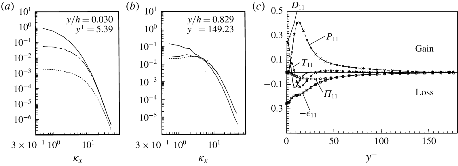
Typical results ensuing from the two approaches above are exemplified in figure 1, where key plots from Kim et al. (Reference Kim, Moin and Moser1987) and from Mansour et al. (Reference Mansour, Kim and Moin1988) are reproduced. Both diagrams stem from the analysis of the same direct numerical simulation database for a turbulent channel flow at small value of Reynolds number ( $Re$). Panels (a,b) are one-dimensional turbulent energy spectra as functions of the streamwise wavenumber, each computed at a specific distance from the wall. Panel (c) shows the wall-normal behaviour of the terms appearing in the budget of the $1,1$ component of the Reynolds stress tensor.
Despite their fundamental importance, both approaches suffer of some limitations. Indeed, it is well known since Richardson (Reference Richardson1922) that turbulence is a truly multi-scale phenomenon, where fluctuations of different spatial extent nonlinearly interact through energy-cascading mechanisms. Even more so, in inhomogeneous flows these interactions vary in space significantly, leading to a transfer of momentum between different spatial locations. The single-point budget equations for the Reynolds stresses do not contain information about the scales involved in such energy fluxes, and therefore miss the multi-scale nature of turbulence. The spectral decomposition and two-point spatial correlations do discern the different scales, but fail to provide direct information on their role in the processes of production, transfer and dissipation of  $k$, and therefore lack a dynamical description of turbulent interactions.
These limitations are overcome when space and scale properties of turbulence are considered jointly. For example, to recover the scale information Lumley (Reference Lumley1964), Domaradzki et al. (Reference Domaradzki, Liu, Härtel and Kleiser1994) and more recently Mizuno (Reference Mizuno2016) and Lee & Moser (Reference Lee and Moser2019) analysed spectrally decomposed budget equations for the Reynolds stresses. They observed inverse energy transfers from small to large scales, supporting substantial modifications of the Richardson scenario in wall-bounded flows. Unfortunately, however, spectral analysis does not allow a definition of scales in statistically inhomogeneous directions, such as the wall-normal one in wall-bounded flows. Hill (Reference Hill2001), Danaila et al. (Reference Danaila, Anselmet, Zhou and Antonia2001), Hill (Reference Hill2002) and Dubrulle (Reference Dubrulle2019) proposed a complementary approach, free from this restriction, and generalised the Kolmogorov (Reference Kolmogorov1941) description of the energy transfer among scales from isotropic flows to inhomogeneous flows.
The generalised Kolmogorov equation or GKE (see for example Danaila, Antonia & Burattini Reference Danaila, Antonia and Burattini2004; Marati, Casciola & Piva Reference Marati, Casciola and Piva2004; Rincon Reference Rincon2006; Cimarelli, De Angelis & Casciola Reference Cimarelli, De Angelis and Casciola2013; Cimarelli et al. Reference Cimarelli, De Angelis, Schlatter, Brethouwer, Talamelli and Casciola2015, Reference Cimarelli, De Angelis, Jimenez and Casciola2016; Portela, Papadakis & Vassilicos Reference Portela, Papadakis and Vassilicos2017) is an exact budget equation for the trace of the so-called second-order structure function tensor, i.e. the sum of the squared increments in all three velocity components between two points in space. This quantity is interpreted as scale energy, and provides scale and space information in every spatial direction, regardless of its statistical homogeneity. The present work discusses the anisotropic generalised Kolmogorov equations (AGKE), which extend the scale and space description of the GKE, limited to scale energy. The goal is to describe each component of the structure function tensor separately, thus capturing the anisotropy of the Reynolds stress tensor and of the underlying budget equations. This provides a complete description of energy redistribution among the various Reynolds stresses. The AGKE identify scales and regions of the flow involved in the production, transfer and dissipation of turbulent stresses, thus integrating the dynamical picture provided by single-point Reynolds stress budgets with the scale information provided by the spectral decomposition. The relationship between the second-order velocity increments and the two-point spatial correlation functions can be exploited to identify the topological features of the structures involved in creation, transport and destruction of turbulent stresses. This endows the kinematic information provided by the spatial correlation functions with additional dynamical information from exact budget equations.
The present work aims at introducing the reader to the AGKE and to their use via example applications to inhomogeneous turbulent flows. The paper is structured as follows. First, in § 2 the budget equations for the structure function tensor are presented and provided with a physical interpretation, and the numerical datasets used in the example flows are described in § 2.2. Then AGKE are applied to canonical turbulent channel flows. In particular, § 3 focuses on the near-wall turbulence cycle of a low- $Re$ channel flow. The energy exchange among the diagonal terms of the structure function tensor via the pressure–strain term is discussed, and the complete AGKE budget of the off-diagonal component is described for the first time. Then, § 4 demonstrates the capability of the AGKE to disentangle the dynamics of flows with a broader range of scales by considering the outer cycle of wall turbulence in channel flows at higher Reynolds numbers. Finally, § 5 considers the separating and reattaching flow over a finite rectangular cylinder, and shows how the AGKE do in such highly inhomogeneous flows. The paper is closed by a brief discussion in § 6. Additional material is reported in three appendices. The complete derivation of the AGKE and their complete form, both in tensorial and component-wise notation, are detailed for reference in appendix A. Appendix B lists the symmetries of the AGKE terms in the specialised form valid for the indefinite plane channel. Appendix C describes the computation of the velocity field induced by the ensemble-averaged quasi-streamwise vortex, employed in § 3.
2 Anisotropic generalised Kolmogorov equations
Let us consider an incompressible turbulent flow, described via its mean and fluctuating velocity fields,  $U_{i}$ and $u_{i}$ respectively, defined after Reynolds decomposition. The AGKE are exact budget equations for the second-order structure function tensor $\left\langle \unicode[STIX]{x1D6FF}u_{i}\unicode[STIX]{x1D6FF}u_{j}\right\rangle$, derived from the Navier–Stokes equations. The operator $\langle \cdot \rangle$ denotes ensemble averaging, as well as averaging along homogeneous directions, if available, and over time if the flow is statistically stationary. The structure function tensor features the velocity increment $\unicode[STIX]{x1D6FF}u_{i}$ of the $i$th velocity component between two points $\boldsymbol{x}$ and $\boldsymbol{x}^{\prime }$ identified by their midpoint $\boldsymbol{X}=(\boldsymbol{x}+\boldsymbol{x}^{\prime })/2$ and separation $\boldsymbol{r}=\boldsymbol{x}^{\prime }-\boldsymbol{x}$, i.e. $\unicode[STIX]{x1D6FF}u_{i}=u_{i}(\boldsymbol{X}+\boldsymbol{r}/2,t)-u_{i}(\boldsymbol{X}-\boldsymbol{r}/2,t)$. (In the following, unless index notation is used, vectors are indicated in bold.)
In the general case,  $\langle \unicode[STIX]{x1D6FF}u_{i}\unicode[STIX]{x1D6FF}u_{j}\rangle$ depends upon seven independent variables, i.e. the six coordinates of the vectors $\boldsymbol{X}$ and $\boldsymbol{r}$ and time $t$, as schematically shown in figure 2, and is related (Davidson, Nickels & Krogstad Reference Davidson, Nickels and Krogstad2006; Agostini & Leschziner Reference Agostini and Leschziner2017) to the variance of the velocity fluctuations (i.e. the Reynolds stresses) and the spatial cross-correlation function as follows:
 $$\begin{eqnarray}\langle \unicode[STIX]{x1D6FF}u_{i}\unicode[STIX]{x1D6FF}u_{j}\rangle (\boldsymbol{X},\boldsymbol{r},t)=V_{ij}(\boldsymbol{X},\boldsymbol{r},t)-R_{ij}(\boldsymbol{X},\boldsymbol{r},t)-R_{ij}(\boldsymbol{X},-\boldsymbol{r},t),\end{eqnarray}$$
where
 $$\begin{eqnarray}V_{ij}(\boldsymbol{X},\boldsymbol{r},t)=\langle u_{i}u_{j}\rangle \left(\boldsymbol{X}+\frac{\boldsymbol{r}}{2},t\right)+\langle u_{i}u_{j}\rangle \left(\boldsymbol{X}-\frac{\boldsymbol{r}}{2},t\right)\end{eqnarray}$$
 is the sum of the single-point Reynolds stresses evaluated at the two points  $\boldsymbol{X}+\boldsymbol{r}/2$ and $\boldsymbol{X}-\boldsymbol{r}/2$ at time $t$, and
 $$\begin{eqnarray}R_{ij}(\boldsymbol{X},\boldsymbol{r},t)=\left\langle u_{i}\left(\boldsymbol{X}+\frac{\boldsymbol{r}}{2},t\right)u_{j}\left(\boldsymbol{X}-\frac{\boldsymbol{r}}{2},t\right)\right\rangle\end{eqnarray}$$
 is the two-point spatial cross-correlation function. The AGKE contains the structural information of  $R_{ij}$; however, for large enough $|\boldsymbol{r}|$ the correlation vanishes, and $\langle \unicode[STIX]{x1D6FF}u_{i}\unicode[STIX]{x1D6FF}u_{j}\rangle$ reduces to $V_{ij}$, whereas the AGKE become the sum of the single-point Reynolds stress budgets at $\boldsymbol{X}\pm \boldsymbol{r}/2$.
Sketch of the quantities involved in the definition of the second-order structure function.  $\boldsymbol{x}=\boldsymbol{X}-\boldsymbol{r}/2$ and $\boldsymbol{x}^{\prime }=\boldsymbol{X}+\boldsymbol{r}/2$ are the two points across which the velocity increment $\unicode[STIX]{x1D6FF}\boldsymbol{u}$ is computed.

2.1 Budget equations
The budget equations for  $\langle \unicode[STIX]{x1D6FF}u_{i}\unicode[STIX]{x1D6FF}u_{j}\rangle$ describe production, transport and dissipation of the turbulent stresses in the compound space of scales and positions, and fully account for the anisotropy of turbulence. For a statistically unsteady turbulent flow, these equations link the variation in time of $\langle \unicode[STIX]{x1D6FF}u_{i}\unicode[STIX]{x1D6FF}u_{j}\rangle$ at a given scale and position, to the instantaneous unbalance among production, inter-component transfer, transport and dissipation. The full derivation starting from the Navier–Stokes equations is detailed in appendix A, and appendix B mentions the symmetries that apply in the plane channel case.
The AGKE can be cast in the following compact form (repeated indices imply summation):
 $$\begin{eqnarray}\frac{\unicode[STIX]{x2202}\langle \unicode[STIX]{x1D6FF}u_{i}\unicode[STIX]{x1D6FF}u_{j}\rangle }{\unicode[STIX]{x2202}t}+\frac{\unicode[STIX]{x2202}\unicode[STIX]{x1D719}_{k,ij}}{\unicode[STIX]{x2202}r_{k}}+\frac{\unicode[STIX]{x2202}\unicode[STIX]{x1D713}_{k,ij}}{\unicode[STIX]{x2202}X_{k}}=\unicode[STIX]{x1D709}_{ij}.\end{eqnarray}$$
 For each  $(i,j)$ pair, $\unicode[STIX]{x1D719}_{k,ij}$ and $\unicode[STIX]{x1D713}_{k,ij}$ are the components in the space of scales $r_{k}$ and in the physical space $X_{k}$ of a six-dimensional vector field of fluxes $\unicode[STIX]{x1D731}_{ij}$, and are given by
 $$\begin{eqnarray}\unicode[STIX]{x1D719}_{k,ij}=\underbrace{\langle \unicode[STIX]{x1D6FF}U_{k}\unicode[STIX]{x1D6FF}u_{i}\unicode[STIX]{x1D6FF}u_{j}\rangle }_{\text{mean}\;\text{transport}}+\underbrace{\langle \unicode[STIX]{x1D6FF}u_{k}\unicode[STIX]{x1D6FF}u_{i}\unicode[STIX]{x1D6FF}u_{j}\rangle }_{\text{turbulent}\;\text{transport}}\underbrace{-2\unicode[STIX]{x1D708}\frac{\unicode[STIX]{x2202}}{\unicode[STIX]{x2202}r_{k}}\langle \unicode[STIX]{x1D6FF}u_{i}\unicode[STIX]{x1D6FF}u_{j}\rangle }_{\text{viscous}\;\text{diffusion}},~~~k=1,2,3,\end{eqnarray}$$
 $$\begin{eqnarray}\displaystyle \unicode[STIX]{x1D713}_{k,ij} & = & \displaystyle \underbrace{\langle {U_{k}}^{\ast }\unicode[STIX]{x1D6FF}u_{i}\unicode[STIX]{x1D6FF}u_{j}\rangle }_{\text{mean}\;\text{transport}}+\underbrace{\langle {u_{k}}^{\ast }\unicode[STIX]{x1D6FF}u_{i}\unicode[STIX]{x1D6FF}u_{j}\rangle }_{\text{turbulent}\;\text{transport}}\nonumber\\ \displaystyle & & \displaystyle +\,\underbrace{\frac{1}{\unicode[STIX]{x1D70C}}\langle \unicode[STIX]{x1D6FF}p\unicode[STIX]{x1D6FF}u_{i}\rangle \unicode[STIX]{x1D6FF}_{kj}+\frac{1}{\unicode[STIX]{x1D70C}}\langle \unicode[STIX]{x1D6FF}p\unicode[STIX]{x1D6FF}u_{j}\rangle \unicode[STIX]{x1D6FF}_{ki}}_{\text{pressure}\;\text{transport}}\underbrace{-\frac{\unicode[STIX]{x1D708}}{2}\frac{\unicode[STIX]{x2202}}{\unicode[STIX]{x2202}X_{k}}\langle \unicode[STIX]{x1D6FF}u_{i}\unicode[STIX]{x1D6FF}u_{j}\rangle }_{\text{viscous}\;\text{diffusion}},\quad k=1,2,3,\end{eqnarray}$$
 and  $\unicode[STIX]{x1D709}_{ij}$ is the source term for $\langle \unicode[STIX]{x1D6FF}u_{i}\unicode[STIX]{x1D6FF}u_{j}\rangle$
 $$\begin{eqnarray}\displaystyle \unicode[STIX]{x1D709}_{ij} & = & \displaystyle \underbrace{-\langle {u_{k}}^{\ast }\unicode[STIX]{x1D6FF}u_{j}\rangle \unicode[STIX]{x1D6FF}\left(\frac{\unicode[STIX]{x2202}U_{i}}{\unicode[STIX]{x2202}x_{k}}\right)-\langle {u_{k}}^{\ast }\unicode[STIX]{x1D6FF}u_{i}\rangle \unicode[STIX]{x1D6FF}\left(\frac{\unicode[STIX]{x2202}U_{j}}{\unicode[STIX]{x2202}x_{k}}\right)}_{\text{production}\;(P_{ij})}\nonumber\\ \displaystyle & & \displaystyle \underbrace{-\langle \unicode[STIX]{x1D6FF}u_{k}\unicode[STIX]{x1D6FF}u_{j}\rangle \left(\frac{\unicode[STIX]{x2202}U_{i}}{\unicode[STIX]{x2202}x_{k}}\right)^{\ast }-\langle \unicode[STIX]{x1D6FF}u_{k}\unicode[STIX]{x1D6FF}u_{i}\rangle \left(\frac{\unicode[STIX]{x2202}U_{j}}{\unicode[STIX]{x2202}x_{k}}\right)^{\ast }}_{\text{production}\;(P_{ij})}\nonumber\\ \displaystyle & & \displaystyle \underbrace{+\frac{1}{\unicode[STIX]{x1D70C}}\left\langle \unicode[STIX]{x1D6FF}p\frac{\unicode[STIX]{x2202}\unicode[STIX]{x1D6FF}u_{i}}{\unicode[STIX]{x2202}X_{j}}\right\rangle +\frac{1}{\unicode[STIX]{x1D70C}}\left\langle \unicode[STIX]{x1D6FF}p\frac{\unicode[STIX]{x2202}\unicode[STIX]{x1D6FF}u_{j}}{\unicode[STIX]{x2202}X_{i}}\right\rangle }_{\text{pressure}\;\text{strain}\;(\unicode[STIX]{x1D6F1}_{ij})}\underbrace{-4{\unicode[STIX]{x1D716}_{ij}}^{\ast }}_{\text{ps.dissipation}\;(D_{ij})}.\end{eqnarray}$$
 Here,  $\unicode[STIX]{x1D6FF}_{ij}$ is the Kronecker delta, $\unicode[STIX]{x1D708}$ is the kinematic viscosity, the asterisk superscript $f^{\ast }$ denotes the average of the generic quantity $f$ between positions $\boldsymbol{X}\pm \boldsymbol{r}/2$ and $\unicode[STIX]{x1D716}_{ij}$ is the pseudo-dissipation tensor, whose trace is the pseudo-dissipation $\unicode[STIX]{x1D716}$. The sum of the equations for the three diagonal components of $\langle \unicode[STIX]{x1D6FF}u_{i}\unicode[STIX]{x1D6FF}u_{j}\rangle$ reduces to the GKE (Hill Reference Hill2001).
Each term contributing to the fluxes in (2.5) and (2.6) can be readily interpreted in analogy with the single-point budget equation for the Reynolds stresses (see e.g. Pope Reference Pope2000) as the mean and turbulent transport, pressure transport and viscous diffusion.  $\unicode[STIX]{x1D753}_{ij}$ describes the flux of $\langle \unicode[STIX]{x1D6FF}u_{i}\unicode[STIX]{x1D6FF}u_{j}\rangle$ among scales, and turbulent transport is the sole nonlinear term; $\unicode[STIX]{x1D74D}_{ij}$ describes the flux of $\langle \unicode[STIX]{x1D6FF}u_{i}\unicode[STIX]{x1D6FF}u_{j}\rangle$ in physical space, and all its terms but the viscous one are nonlinear. The source term $\unicode[STIX]{x1D709}_{ij}$ describes the net production of $\langle \unicode[STIX]{x1D6FF}u_{i}\unicode[STIX]{x1D6FF}u_{j}\rangle$ in space and among scales; it is similar to the one appearing in the GKE, but additionally features a pressure–strain term, involved in the energy redistribution process between different components of turbulent stresses. Each term in (2.4) informs on the spatial position $\boldsymbol{X}$, scale $\boldsymbol{r}$ and time $t$ at which production, transport and dissipation of Reynolds stresses are statistically important.
The diagonal components of  $\langle \unicode[STIX]{x1D6FF}u_{i}\unicode[STIX]{x1D6FF}u_{j}\rangle$ are positive by definition, and their budget equations inherit the interpretation proposed by Marati et al. (Reference Marati, Casciola and Piva2004) and Cimarelli et al. (Reference Cimarelli, De Angelis and Casciola2013) for the GKE: they are analogous to scale energy, and the AGKE enable their discrimination into the separate diagonal components of the Reynolds stress tensor. The non-diagonal components, however, can in general assume positive or negative values, also when the sign of $\langle u_{i}u_{j}\rangle$ can be predicted on physical grounds. For these components, $\unicode[STIX]{x1D709}_{ij}$ has the generic meaning of a source term, which can be viewed as production or dissipation only upon considering the actual sign of $\langle \unicode[STIX]{x1D6FF}u_{i}\unicode[STIX]{x1D6FF}u_{j}\rangle$ at the particular values of $(\boldsymbol{X},\boldsymbol{r})$. In analogy with the concept of energy cascade, paths of $\langle \unicode[STIX]{x1D6FF}u_{i}\unicode[STIX]{x1D6FF}u_{j}\rangle$ in the $(\boldsymbol{X},\boldsymbol{r})$ space represent fluxes of Reynolds stresses through space ( $\boldsymbol{X}$) and scales ( $\boldsymbol{r}$) at time $t$. The shape of the paths is determined by $\unicode[STIX]{x1D74D}_{ij}$ (space fluxes) and $\unicode[STIX]{x1D753}_{ij}$ (scale fluxes).
2.2 Simulations and databases
Details of the three turbulent channel flow direct numerical simulation databases. For each  $Re_{\unicode[STIX]{x1D70F}}$, the table provides the computed value of the friction coefficient $C_{f}=2(u_{\unicode[STIX]{x1D70F}}/U_{b})^{2}$, the size of the computational domain, number of Fourier modes and collocation points in the wall-normal direction, spatial resolution (computed after the $3/2$-rule dealiasing in the homogeneous directions), the number $N$ of accumulated flow snapshots and their temporal spacing $\unicode[STIX]{x0394}t$. The cases at $Re_{\unicode[STIX]{x1D70F}}=200$ and $Re_{\unicode[STIX]{x1D70F}}=1000$ were already documented by Gatti & Quadrio (Reference Gatti and Quadrio2016) and Gatti et al. (Reference Gatti, Cimarelli, Hasegawa, Frohnapfel and Quadrio2018).

As anticipated in § 1, the AGKE analysis below stems from the post-processing of velocity and pressure fields obtained via direct numerical simulations (DNS) of two flows. The former is the turbulent plane channel flow, whose inner and outer turbulent cycles will be discussed in § 3 and § 4 respectively. The latter is the separating and reattaching flow around a finite rectangular cylinder, discussed in § 5.
The turbulent channel flow simulations have been carried out for the present work via the DNS code introduced by Luchini & Quadrio (Reference Luchini and Quadrio2006). The incompressible Navier–Stokes equations are projected in the divergence-free space of the wall-normal components of the velocity and vorticity vectors and solved by means of a pseudo-spectral method, as in Kim et al. (Reference Kim, Moin and Moser1987). Three database are used, with friction Reynolds numbers  $Re_{\unicode[STIX]{x1D70F}}=u_{\unicode[STIX]{x1D70F}}h/\unicode[STIX]{x1D708}$ of $Re_{\unicode[STIX]{x1D70F}}=200$, $500$ and $1000$. Here, $h$ is the channel half-height, and $u_{\unicode[STIX]{x1D70F}}=\sqrt{\unicode[STIX]{x1D70F}_{w}/\unicode[STIX]{x1D70C}}$ is the friction velocity expressed in terms of the average wall shear stress $\unicode[STIX]{x1D70F}_{w}$ and the density $\unicode[STIX]{x1D70C}$. The size of the computational domain is $L_{x}=4\unicode[STIX]{x03C0}h$ and $L_{z}=2\unicode[STIX]{x03C0}h$ in the streamwise and spanwise directions, discretised by $N_{x}=N_{z}=256$, $512$ and $1024$ Fourier modes (further increased by a factor $3/2$ for de-aliasing). In the wall-normal direction the differential operators are discretised via fourth-order compact finite differences using respectively $N_{y}=256$, $250$ and $500$ points collocated on a non-uniform grid. Further details are provided in table 1. In this table and throughout the whole paper, quantities denoted with the superscript $+$ are given in viscous units, i.e. normalised with $u_{\unicode[STIX]{x1D70F}}$ and $\unicode[STIX]{x1D708}$.
The database for the flow around a finite rectangular cylinder is taken from the DNS study by Cimarelli et al. (Reference Cimarelli, Leonforte and Angeli2018), where the information on the numerical set-up can be found. A rectangular cylinder of length  $5h$, thickness $h$ and indefinite span is immersed in a uniform flow with free-stream velocity $U_{\infty }$ aligned with the $x$ direction. The Reynolds number is $Re=U_{\infty }h/\unicode[STIX]{x1D708}=3000$. The streamwise, wall-normal and spanwise size of the computation domain is $(L_{x},L_{y},L_{z})=(112h,50h,5h)$. The leading edge of the cylinder is located $35h$ past the inlet of the computational box. The fluid domain is discretised through a Cartesian grid consisting of $1.5\times 10^{7}$ hexahedral cells. The average resolution in the three spatial direction is $(\unicode[STIX]{x0394}x^{+},\unicode[STIX]{x0394}y^{+},\unicode[STIX]{x0394}z^{+})=(6.1,0.31,5.41)$.
The AGKE terms are computed with an efficient code specifically developed for the present work, which extends a recently written code for the computation of the GKE equation (Gatti et al. Reference Gatti, Remigi, Chiarini, Cimarelli and Quadrio2019). The symmetries described in appendix B are exploited to minimise the amount of memory required during the calculations. Each term of (2.5), (2.6) and (2.7) is decomposed into simpler correlation terms, which are then computed as products in Fourier space along the homogeneous directions, with huge savings in computing time. For maximum accuracy, derivatives in the homogeneous directions are computed in the Fourier space, otherwise a finite-differences scheme with a five-points computational stencil is used. Finally, a parallel strategy is implemented (see Gatti et al. Reference Gatti, Remigi, Chiarini, Cimarelli and Quadrio2019, for details). The calculation receives in input the fluctuating velocity field for each snapshot of the databases. It outputs  $\langle \unicode[STIX]{x1D6FF}u_{i}\unicode[STIX]{x1D6FF}u_{j}\rangle$, the flux vectors $\unicode[STIX]{x1D74D}_{ij}$ and $\unicode[STIX]{x1D753}_{ij}$, and the various contributions to the source term $\unicode[STIX]{x1D709}_{ij}$ as in (2.7) for each of the six different second-order structure functions, and in the whole physical and scale space.
The statistical convergence of the data is verified by ensuring that the residual of equation (2.4) is negligible compared to the dissipation, production and pressure–strain terms.
3 Example: the near-wall turbulence cycle
A turbulent channel flow at  $Re_{\unicode[STIX]{x1D70F}}=200$ is considered in the following. The mean velocity vector is $\boldsymbol{U}\left(y\right)=\left\{U(y),0,0\right\}$, directed along the streamwise direction $x=x_{1}$ and varying only with the wall-normal coordinate $y=x_{2}$, while $z=x_{3}$ denotes the spanwise direction, and $u=u_{1}$, $v=u_{2}$ and $w=u_{3}$ indicate the three fluctuating velocity components. Since $y$ is the only direction of statistical inhomogeneity, $\langle \unicode[STIX]{x1D6FF}u_{i}\unicode[STIX]{x1D6FF}u_{j}\rangle (Y,\boldsymbol{r})$ and all AGKE terms are functions of the physical space only through the spatial coordinate $Y=(y+y^{\prime })/2$, while still depending upon the whole scale vector $\boldsymbol{r}$. Similarly, spatial transport of $\langle \unicode[STIX]{x1D6FF}u_{i}\unicode[STIX]{x1D6FF}u_{j}\rangle$ occurs along $Y$ through the only non-zero component of the spatial flux $\unicode[STIX]{x1D713}_{ij}=\unicode[STIX]{x1D713}_{Y,ij}$.
The GKE for the scale energy  $\langle \unicode[STIX]{x1D6FF}u_{i}^{2}\rangle$ has been thoroughly discussed in the literature, (see e.g. Marati et al. Reference Marati, Casciola and Piva2004; Cimarelli et al. Reference Cimarelli, De Angelis and Casciola2013, Reference Cimarelli, De Angelis, Schlatter, Brethouwer, Talamelli and Casciola2015, Reference Cimarelli, De Angelis, Jimenez and Casciola2016), and different interpretations and visualisation techniques have been suggested. For this reason, in the following we only address the new information offered by the AGKE. This includes the analysis of the anisotropic scale-energy redistribution operated by the pressure–strain terms, and that of the budget equation for $\langle -\unicode[STIX]{x1D6FF}u\unicode[STIX]{x1D6FF}v\rangle$. The analysis is also restricted to the subspace $r_{x}=0$: this is motivated by the turbulent vortical structures in channel flow being predominantly aligned in the streamwise direction. Such structures typically induce the largest negative correlation of velocity components for $r_{x}=0$ and characteristic values of $r_{z}$. A classic example are the so-called near-wall streaks, for which $r_{z}^{+}\approx 60$. As a consequence of (2.1), the local maxima of, for instance, $\langle \unicode[STIX]{x1D6FF}u\unicode[STIX]{x1D6FF}u\rangle$ and terms appearing in its budget equation also occur for $r_{x}\approx 0$. Note that in the $r_{x}=0$ space the terms of the AGKE are not defined below the $Y=r_{y}/2$ plane, owing to the finite size of the channel in the wall-normal direction.
3.1 Scale-energy redistribution by pressure strain
The pressure–strain term  $\unicode[STIX]{x1D6F1}_{ij}$ redistributes energy among the diagonal components of $\langle \unicode[STIX]{x1D6FF}u_{i}\unicode[STIX]{x1D6FF}u_{j}\rangle$. Hence, at different scales and positions this term can be a source or a sink depending on its sign. To better understand its behaviour and link it to physical processes, it is instructive to briefly analyse the scales and position at which $\langle \unicode[STIX]{x1D6FF}u\unicode[STIX]{x1D6FF}u\rangle$, $\langle \unicode[STIX]{x1D6FF}v\unicode[STIX]{x1D6FF}v\rangle$, $\langle \unicode[STIX]{x1D6FF}w\unicode[STIX]{x1D6FF}w\rangle$ and their sources $\unicode[STIX]{x1D709}_{ij}$ are important.
The position and the intensity of the maxima, hereinafter denoted with the subscript  $m$, of the diagonal components of $\langle \unicode[STIX]{x1D6FF}u_{i}\unicode[STIX]{x1D6FF}u_{j}\rangle$ and of the associated $\unicode[STIX]{x1D709}_{ij}$ and $\unicode[STIX]{x1D6F1}_{ij}$ are reported in table 2. $\langle \unicode[STIX]{x1D6FF}u\unicode[STIX]{x1D6FF}u\rangle$, $\langle \unicode[STIX]{x1D6FF}v\unicode[STIX]{x1D6FF}v\rangle$ and $\langle \unicode[STIX]{x1D6FF}w\unicode[STIX]{x1D6FF}w\rangle$ peak at small scales within the buffer layer, similarly to $\langle \unicode[STIX]{x1D6FF}u_{i}^{2}\rangle$ (Cimarelli et al. Reference Cimarelli, De Angelis, Jimenez and Casciola2016), with $\langle \unicode[STIX]{x1D6FF}v\unicode[STIX]{x1D6FF}v\rangle _{m}$ located further from the wall. The anisotropy of the flow is denoted, for instance, by $\langle \unicode[STIX]{x1D6FF}w\unicode[STIX]{x1D6FF}w\rangle _{m}$ being much lower than $\langle \unicode[STIX]{x1D6FF}u\unicode[STIX]{x1D6FF}u\rangle _{m}$ and occurring at $r_{z}=0$ and small $r_{y}$, whereas the other maxima occur at $r_{z}\neq 0$ and $r_{y}=0$. This difference is explained by the quasi-streamwise vortices populating the near-wall cycle (Schoppa & Hussain Reference Schoppa and Hussain2002): they induce negatively correlated regions of spanwise fluctuations at $r_{y}\neq 0$ and of streamwise and wall-normal fluctuations at $r_{z}\neq 0$.
The region of negative source terms partially coincides with the one of the source term in the GKE (see e.g. Cimarelli et al. Reference Cimarelli, De Angelis, Jimenez and Casciola2016). As in the GKE, negative sources are observed at the lower boundary  $Y=r_{y}/2$, and in the whole channel height at $r_{y},r_{z}\rightarrow 0$: viscous dissipation dominates near the wall and at the smallest scales. However, the regions of large positive sources vary significantly among the three diagonal components (see table 2). This is due to the different nature of the positive source of the three diagonal components of $\langle \unicode[STIX]{x1D6FF}u_{i}\unicode[STIX]{x1D6FF}u_{j}\rangle$. Indeed, in a turbulent channel flow the streamwise fluctuations are fed by the energy draining from the mean flow (i.e. by the production term $P_{11}$), whereas the cross-stream fluctuations are produced by the redistribution processes (i.e. the pressure–strain term $\unicode[STIX]{x1D6F1}_{22}$ and $\unicode[STIX]{x1D6F1}_{33}$). This explains also the larger order of magnitude of $\unicode[STIX]{x1D709}_{11,m}$. Unlike the GKE, the scale and space properties of this energy redistribution can be extracted from the AGKE (see (2.7)).
Colour plot of  $\unicode[STIX]{x1D6F1}_{11}^{+}$ (a), $\unicode[STIX]{x1D6F1}_{22}^{+}$ (b) and $\unicode[STIX]{x1D6F1}_{33}^{+}$ (c) on the bounding planes $r_{y}^{+}=0$, $r_{z}^{+}=0$ and $Y^{+}=r_{y}^{+}/2$. The contour lines increment is 0.04, with level zero indicated by a thick line. The two symbols identify the positions of the maxima of $\unicode[STIX]{x1D6F1}_{ij}$ (cross) and $P_{ij}$ (circle). The isosurface in (a) corresponds to $\unicode[STIX]{x1D6F1}_{22}/\unicode[STIX]{x1D6F1}_{11}=-0.5$ (or equivalently $\unicode[STIX]{x1D6F1}_{33}/\unicode[STIX]{x1D6F1}_{11}=-0.5$), with $\unicode[STIX]{x1D6F1}_{22}/\unicode[STIX]{x1D6F1}_{11}<-0.5$ for smaller scales.

Maximum values for diagonal terms of  $\langle \unicode[STIX]{x1D6FF}u_{i}\unicode[STIX]{x1D6FF}u_{j}\rangle ^{+}$, its source $\unicode[STIX]{x1D709}_{ij}^{+}$, absolute pressure strain $|\unicode[STIX]{x1D6F1}_{ij}^{+}|$ and production $P_{ij}^{+}$ and positions in the $(r_{y}^{+},r_{z}^{+},Y^{+})$-space.
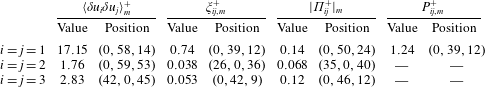
Figure 3 plots the pressure–strain term for the diagonal components, with values and positions of their maxima as reported in table 2. The figure shows the location of the pressure–strain maximum in absolute value together with the maximum production. Large values of  $P_{11}$ occur near the plane $Y^{+}=r_{y}^{+}/2+14$, except for the smallest scales in the region $r_{y}^{+}<30$ and $r_{z}^{+}<20$. On the other hand, $\unicode[STIX]{x1D6F1}_{11}$ is negative almost everywhere, showing that the streamwise fluctuations lose energy at all scales to feed the other components. In particular, large negative values of $\unicode[STIX]{x1D6F1}_{11}$, albeit much smaller than $P_{11}$, are seen near the plane $Y^{+}=r_{y}^{+}/2+24$, except for the region $r_{y}^{+},r_{z}^{+}<20$. This brings to light the dominant scales and wall distances involved in the process of redistribution of $\langle \unicode[STIX]{x1D6FF}u\unicode[STIX]{x1D6FF}u\rangle$ towards the other components, and discriminates them from those involved in its production. On the contrary, at the smallest scales where viscous dissipation is dominant production and redistribution are not observed.
The pressure–strain terms of the cross-stream components,  $\unicode[STIX]{x1D6F1}_{22}$ and $\unicode[STIX]{x1D6F1}_{33}$, are positive almost everywhere; they show a positive peak near the wall and remain larger than dissipation in different regions of the $r_{x}=0$ space. Their maxima are located in the vicinity of the plane $Y^{+}=r_{y}^{+}/2+40$ for $\unicode[STIX]{x1D6F1}_{22}$ and $Y^{+}=r_{y}^{+}/2+14$ for $\unicode[STIX]{x1D6F1}_{33}$, where $\unicode[STIX]{x1D6F1}_{11}$ is negative. Hence, at these scales and wall-normal distances $\langle \unicode[STIX]{x1D6FF}u\unicode[STIX]{x1D6FF}u\rangle$ loses energy to $\langle \unicode[STIX]{x1D6FF}v\unicode[STIX]{x1D6FF}v\rangle$ and $\langle \unicode[STIX]{x1D6FF}w\unicode[STIX]{x1D6FF}w\rangle$. Moreover, $\unicode[STIX]{x1D6F1}_{22}$ is negative in the very near-wall region, $Y^{+}<r_{y}^{+}/2+5$, owing to the non-penetration wall boundary condition which converts $\langle \unicode[STIX]{x1D6FF}v\unicode[STIX]{x1D6FF}v\rangle$ into $\langle \unicode[STIX]{x1D6FF}u\unicode[STIX]{x1D6FF}u\rangle$ and $\langle \unicode[STIX]{x1D6FF}w\unicode[STIX]{x1D6FF}w\rangle$. Indeed, here $\unicode[STIX]{x1D6F1}_{11}$ and $\unicode[STIX]{x1D6F1}_{33}$ are positive. This phenomenon is known as the splatting effect (Mansour et al. Reference Mansour, Kim and Moin1988), and shows no scale dependency.
Different values of  $\unicode[STIX]{x1D6F1}_{22}$ and $\unicode[STIX]{x1D6F1}_{33}$ imply an anisotropic redistribution of the streamwise fluctuations to the other components. Owing to the incompressibility constraint, the following relationship holds:
 $$\begin{eqnarray}\frac{\unicode[STIX]{x1D6F1}_{22}}{\unicode[STIX]{x1D6F1}_{11}}+\frac{\unicode[STIX]{x1D6F1}_{33}}{\unicode[STIX]{x1D6F1}_{11}}=-1.\end{eqnarray}$$
 Hence,  $\unicode[STIX]{x1D6F1}_{22}/\unicode[STIX]{x1D6F1}_{11}=\unicode[STIX]{x1D6F1}_{33}/\unicode[STIX]{x1D6F1}_{11}=-0.5$ corresponds to isotropic transfer of energy from the streamwise fluctuations towards the other components. In figure 3(a) the isosurface $\unicode[STIX]{x1D6F1}_{22}/\unicode[STIX]{x1D6F1}_{11}=-0.5$ is shown. The inner side at small scales of this surface is characterised by $\unicode[STIX]{x1D6F1}_{22}/\unicode[STIX]{x1D6F1}_{11}<-0.5$, and thus by $\unicode[STIX]{x1D6F1}_{22}>\unicode[STIX]{x1D6F1}_{33}$ (as long as $\unicode[STIX]{x1D6F1}_{11}<0$). Hence, at small scales the pressure strain preferentially redistributes streamwise energy to the vertical fluctuations. On the contrary, on the outer side of the surface $\unicode[STIX]{x1D6F1}_{33}>\unicode[STIX]{x1D6F1}_{22}$ holds, implying that at larger scales the streamwise energy is preferentially redistributed towards spanwise fluctuations.
3.2 Scale-by-scale budget of the off-diagonal term  $\langle -\unicode[STIX]{x1D6FF}u\unicode[STIX]{x1D6FF}v\rangle$

The only off-diagonal term associated with a non-zero component of the Reynolds stress tensor is  $\langle -\unicode[STIX]{x1D6FF}u\unicode[STIX]{x1D6FF}v\rangle$ which, unlike the diagonal terms, is not definite in sign. Therefore, $\langle -\unicode[STIX]{x1D6FF}u\unicode[STIX]{x1D6FF}v\rangle$ and its fluxes cannot be interpreted in terms of energy and energy transfer; $\langle -\unicode[STIX]{x1D6FF}u\unicode[STIX]{x1D6FF}v\rangle$ describes the statistical dependence or, more precisely, the correlation between $\unicode[STIX]{x1D6FF}u$ and $\unicode[STIX]{x1D6FF}v$ and, for large $\boldsymbol{r}$, the mean momentum transfer. Concepts as production and dissipation only apply to the source term $\unicode[STIX]{x1D709}_{12}$ after the sign of $\langle -\unicode[STIX]{x1D6FF}u\unicode[STIX]{x1D6FF}v\rangle$ is taken into account.
Colour plot of  $\langle -\unicode[STIX]{x1D6FF}u\unicode[STIX]{x1D6FF}v\rangle$ and its budget terms in the three-dimensional space $r_{x}=0$. (a) $\langle -\unicode[STIX]{x1D6FF}u\unicode[STIX]{x1D6FF}v\rangle ^{+}$: contour lines increment by 0.4, with zero indicated by a thick line. (b) Colour plot of $\unicode[STIX]{x1D709}_{12}^{+}$: contour lines increment by 0.02, with zero indicated by a thick line. The grey lines are tangent to the flux vector $(\unicode[STIX]{x1D719}_{y},\unicode[STIX]{x1D719}_{z},\unicode[STIX]{x1D713})$ and coloured with its magnitude. A zoom of the region near the origin is shown in panel (d). (c) Colour plot of $P_{12}^{+}$ in the $r_{x}=r_{y}=0$ plane, with isolines for $\unicode[STIX]{x1D6F1}_{12}^{+}$ demonstrating the different scales involved and the different position of the maximum. The $\times$ symbol gives the position of the maximum for $\unicode[STIX]{x1D6F1}_{12}$.

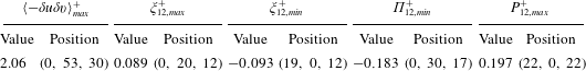
Maximum value for  $\langle -\unicode[STIX]{x1D6FF}u\unicode[STIX]{x1D6FF}v\rangle ^{+}$, maximum and minimum for the source $\unicode[STIX]{x1D709}_{12}^{+}$, minimum for the pressure strain $\unicode[STIX]{x1D6F1}_{12}^{+}$ and maximum of the production $P_{12}^{+}$ and positions in the $(r_{y}^{+},r_{z}^{+},Y^{+})$-space.
3.2.1 Intensity, production and redistribution
The off-diagonal term  $\langle -\unicode[STIX]{x1D6FF}u\unicode[STIX]{x1D6FF}v\rangle$ and its budget are plotted in figure 4, and corresponding quantitative information is reported in table 3. As shown by figure 4(a), $\langle -\unicode[STIX]{x1D6FF}u\unicode[STIX]{x1D6FF}v\rangle$ is positive almost throughout the entire physical/scale space except at very small separations ( $r_{z}^{+}=0,r_{y}\leqslant 10$) for $Y^{+}<50$. The largest positive values of $\langle -\unicode[STIX]{x1D6FF}u\unicode[STIX]{x1D6FF}v\rangle$ are in the buffer layer at $15\leqslant Y^{+}\leqslant 60$, at spanwise scales $40\leqslant r_{z}^{+}\leqslant 80$ and vanishing $r_{y}$. A second, less prominent local maximum of $\langle -\unicode[STIX]{x1D6FF}u\unicode[STIX]{x1D6FF}v\rangle$ is located near the $r_{z}=0$ plane.
The source term  $\unicode[STIX]{x1D709}_{12}$, plotted in figure 4(b), is dominated by the (positive) production term $P_{12}$ and the (negative) pressure–strain term $\unicode[STIX]{x1D6F1}_{12}$ (see (A 17) for their definitions). Indeed, the viscous pseudo-dissipation $D_{12}$ plays a minor role, as in the single-point budget for $\langle -uv\rangle$ (see e.g. Mansour et al. Reference Mansour, Kim and Moin1988). Large positive and negative values of $\unicode[STIX]{x1D709}_{12}$ define two distinct regions in the buffer layer (figure 4d). The positive peak corresponds to spanwise scales $10\leqslant r_{z}^{+}\leqslant 50$, while the negative one to small scales ( $r_{z}^{+}\approx 0$). Moreover, $\unicode[STIX]{x1D709}_{12}$ is negative in a portion of the $Y^{+}=r_{y}^{+}/2$ plane, implying that turbulent structures extending down to the wall are inactive in the production of $\langle -\unicode[STIX]{x1D6FF}u\unicode[STIX]{x1D6FF}v\rangle$.
Source term  $\unicode[STIX]{x1D709}_{12}$ in the $r_{y}=0$ plane. (a) $\unicode[STIX]{x1D709}_{12}^{+}$ versus $Y^{+}$ for different $r_{z}^{+}=(10:10:100)$. (b) $\unicode[STIX]{x1D709}_{12}^{+}$ versus $r_{z}^{+}$ for different $Y^{+}=(10:5:50)$. Line colours encode the value of the parameter, which increases from yellow (light) to red (dark).

It is worth noting that  $\unicode[STIX]{x1D709}_{12}$ strongly varies with spanwise separation, as seen in the $r_{y}=0$ plane (figure 4c; see also figure 5). In comparison to the global picture obtained from single-point analysis of $\langle -uv\rangle$ in the buffer layer (here recovered in the limit $r_{z}\rightarrow L_{z}/2$) where the source term is slightly negative, one can additionally appreciate the existence of a large positive peak of $\unicode[STIX]{x1D709}_{12}$ at $r_{z}^{+}=20$ and a negative one at $r_{z}^{+}=70$ (figure 5b). Indeed, $P_{12}$ and $\unicode[STIX]{x1D6F1}_{12}$ are of the same order of magnitude throughout the $r_{y}=0$ plane, but reach their extreme values at different spanwise scales, see figure 4(c). In particular large values of $P_{12}$ are found at $(r_{z}^{+},Y^{+})\approx (30,17)$, whereas large negative values of $\unicode[STIX]{x1D6F1}_{12}$ are found at $(r_{z}^{+},Y^{+})\approx (60,16)$. The structural interpretation of these findings is discussed below in § 3.2.3.
3.2.2 Fluxes
The transfer of  $\langle -\unicode[STIX]{x1D6FF}u\unicode[STIX]{x1D6FF}v\rangle$ in space and among scales is determined by the flux vector $(\unicode[STIX]{x1D719}_{y},\unicode[STIX]{x1D719}_{z},\unicode[STIX]{x1D713})$, and is visualised via its field lines. These field lines can be grouped in two families. The lines of the first family enter the domain from the channel centreline, $Y=h$, and descend towards the wall; they can be further grouped in sets I, II and III as shown in figure 4(b). The second family only contains set IV, and is visible in the zoomed figure 4(d); its field lines are confined to the near-wall region, and connect the positive and negative peaks of $\unicode[STIX]{x1D709}_{12}$.
Field lines of the flux vector for  $\langle -\unicode[STIX]{x1D6FF}u\unicode[STIX]{x1D6FF}v\rangle$. (a–c) Set I; (d–f) Set II; (g–i) Set IV. (a,d,g) Evolution of the values of $Y$ (– $\cdot$– $\cdot$–, dark green), $r_{y}$ (——, blue), $r_{z}$ (— –, red), along a representative field line as a function of its dimensionless arc length $s$. (b,e,h) Values of $\langle -\unicode[STIX]{x1D6FF}u\unicode[STIX]{x1D6FF}v\rangle /10$ (– $\cdot$– $\cdot$–, dark green), $\unicode[STIX]{x1D709}_{12}$ (— –, red), $P_{12}$ ( $\cdots \cdots$), $D_{12}$ (——, blue) and $\unicode[STIX]{x1D6F1}_{12}$ (- - - -, grey) along the line. (c,f,i) Evolution of $-\unicode[STIX]{x1D70C}_{12}$ (——) and $-\unicode[STIX]{x1D70C}_{21}$ (- - - -) along the line.

Various quantities can be tracked along representative field lines, as done in figure 6. The position along a field line of length  $\ell$ in the $(r_{z},r_{y},Y)$ space is described by the normalised curvilinear coordinate
 $$\begin{eqnarray}s=\frac{1}{\ell }\int _{0}^{\ell }\text{d}s\quad \text{with}~\text{d}s=\sqrt{\text{d}r_{z}^{2}+\text{d}r_{y}^{2}+\text{d}Y^{2}}.\end{eqnarray}$$
 The values of  $r_{y}$, $r_{z}$ and $Y$ (see figure 2) are plotted in the left column of the figure; the central column plots the evolution of $\langle -\unicode[STIX]{x1D6FF}u\unicode[STIX]{x1D6FF}v\rangle$, $\unicode[STIX]{x1D709}_{12}$, $P_{12}$, $\unicode[STIX]{x1D6F1}_{12}$ and the dissipation $D_{12}$ along the line; the right column plots the evolution of the correlation coefficient $\unicode[STIX]{x1D70C}_{ij}$ defined by
 $$\begin{eqnarray}\unicode[STIX]{x1D70C}_{ij}=\frac{R_{ij}(Y,r_{y},r_{z})}{\sqrt{\langle u_{i}u_{i}\rangle (Y)\langle u_{j}u_{j}\rangle (Y)}},\end{eqnarray}$$
 where repeated indices do not imply summation;  $R_{ij}$ is linked to $\langle \unicode[STIX]{x1D6FF}u_{i}\unicode[STIX]{x1D6FF}u_{j}\rangle$ by equation (2.1).
Figures 6(a–c) and 6(d–f) illustrate the evolution of various quantities along representative lines of set I and II. Both lines are qualitatively similar: they highlight a transfer of  $\langle -\unicode[STIX]{x1D6FF}u\unicode[STIX]{x1D6FF}v\rangle$ from the centreline to the near-wall region, through first decreasing and then increasing wall-normal scales. At the centreline they are parallel to the $Y$ axis, consistently with the AGKE symmetries (see appendix B). However, lines of set I are attracted by the negative peak of $\unicode[STIX]{x1D709}_{12}$ towards smaller $r_{z}$, while those of set II are repulsed from the positive source peak towards larger $r_{z}$. Lines of set III are not shown for the sake of brevity, since they pass through regions of large separations and are characterised by almost zero correlation, see (3.3). On the other hand, lines of sets I and II exist at smaller $r_{y}$ and $r_{z}$ and, as shown in figures 6(c) and 6(f), are characterised by finite levels of correlation. Along lines of set I and II, $\langle -\unicode[STIX]{x1D6FF}u\unicode[STIX]{x1D6FF}v\rangle$ increases from zero at the centreline (due to the AGKE symmetries) to reach a positive peak in the near-wall region. Similarly, $\unicode[STIX]{x1D709}_{12}$ shows a negative/positive peak when the lines of set I/II approach the near-wall region as the pressure–strain/production overcomes the production/pressure–strain.
The evolution of the correlation coefficients  $-\unicode[STIX]{x1D70C}_{12}$ and $-\unicode[STIX]{x1D70C}_{21}$ (recall that $\unicode[STIX]{x1D70C}_{ij}\neq \unicode[STIX]{x1D70C}_{ji}$ for $i\neq j$, see (3.3)) is used to extract information about the turbulent structures involved in production, transfer and dissipation processes highlighted along the lines. As shown in figures 6(a) and 6(d), at values of the curvilinear coordinate $s>0.75$ corresponding to $Y^{+}<60$, lines of set I intersect positive $-\unicode[STIX]{x1D70C}_{12}$ and $-\unicode[STIX]{x1D70C}_{21}$ for small $r_{z}$ and $r_{y}$, while those of set II intersect negative correlations at larger $r_{z}^{+}\sim 50$ and smaller $r_{y}$. For both sets, this is consistent with the flow field induced by near-wall quasi-streamwise vortices, creating positive and negative cross-correlation at values of separation in agreement with the present analysis; positive $-\unicode[STIX]{x1D70C}_{12}$ is associated with $u$ and $v$ fluctuations at the same-side of the vortices (i.e. small $r_{z}$), whereas negative $-\unicode[STIX]{x1D70C}_{12}$ is associated with opposite-side fluctuations. Hence, we relate the peaks of $P_{12}$ and $\unicode[STIX]{x1D6F1}_{12}$ (and consequently of $\unicode[STIX]{x1D709}_{12}$) along the lines of sets I and II to such structures.
The lines of set IV, shown in figure 4(b,d) and in figure 6(g–i), behave differently. The field lines originate in the lower boundary of the domain at  $(r_{y}^{+},r_{z}^{+},Y^{+})=(6,15,3)$. Along their path they first intercept the positive peak of $\unicode[STIX]{x1D709}_{12}$ at small $r_{y}$ where $\langle -\unicode[STIX]{x1D6FF}u\unicode[STIX]{x1D6FF}v\rangle$ is maximum. Then, they pass through the negative peak of $\unicode[STIX]{x1D709}_{12}$, located at smaller $r_{z}$ and larger $r_{y}$, where $\langle -\unicode[STIX]{x1D6FF}u\unicode[STIX]{x1D6FF}v\rangle$ is smaller. Eventually, they again vanish in the lower boundary of the domain.
Focusing on the correlation coefficient  $-\unicode[STIX]{x1D70C}_{12}$, lines of set IV intersect a positive value along their complete extension. In detail, the lines first intersect small values of $-\unicode[STIX]{x1D70C}_{12}$ for $r_{z}^{+}\approx 20$ and $Y^{+}<5$ and then larger $-\unicode[STIX]{x1D70C}_{12}$ for smaller $r_{z}^{+}$ and larger $Y^{+}$. Hence, this set of lines highlights a transfer of $\langle -\unicode[STIX]{x1D6FF}u\unicode[STIX]{x1D6FF}v\rangle$ between the small $uv$-structures created in the viscous sublayer by the wall boundary condition (Sillero et al. Reference Sillero, Jiménez and Moser2014) and the turbulent structures of the near-wall cycle.
3.2.3 Structural properties of wall turbulence
(a) Ensemble-average quasi-streamwise vortex, educed as described in § 3.2.3 and appendix C, represented as isosurface  $\unicode[STIX]{x1D706}_{ci}^{+}=0.145$ of the swirling strength criterion (Zhou et al. Reference Zhou, Adrian, Balachandar and Kendall1999). The coherent streamwise (black) and wall-normal (red) velocity field induced by the vortex are plotted on a $(y,z)$ plane, located at $x=0$, passing through the centre of the vortex. The plane is represented both in (a) and, more in detail, in (b). Contour levels at $(0.2:0.2:0.8)$ of the maximum (solid line) and of the minimum (dashed line) of the respective component ( $0.0058$ and $-0.0077$ for $u$ and $0.0035$ and $-0.0035$ for $v$) are plotted on a $(y,z)$ plane passing through the centre of the vortex, located at $z=0$. (c) Colour map of the corresponding $\langle \unicode[STIX]{x1D6FF}u\unicode[STIX]{x1D6FF}v\rangle$ normalised by its maximum value on the plane $r_{x}=r_{y}=0$. (d) Colour map of the corresponding $P_{12}$, and contours of $\unicode[STIX]{x1D6F1}_{12}$, normalised by its maximum value, on the plane $r_{x}=r_{y}=0$. Contours levels are shown at ( $-0.6$, $-0.7$), and the $\times$ symbols locates the maximum.

To connect the main statistical features of  $\langle -\unicode[STIX]{x1D6FF}u\unicode[STIX]{x1D6FF}v\rangle$ in the buffer layer to the turbulent structures that populate it, we compute the $\langle -\unicode[STIX]{x1D6FF}u\unicode[STIX]{x1D6FF}v\rangle$ AGKE budget from the velocity field induced by the ensemble-averaged quasi-streamwise vortex. Such vortex, visualised in figure 7(a), represents the characteristic near-wall coherent structure in the average sense. The procedure which extracts the ensemble-average vortical structure from the DNS database is very similar to the one presented by Jeong et al. (Reference Jeong, Hussain, Schoppa and Kim1997), which is slightly modified here to focus on the structures in the buffer layer only. Details of the procedure are provided in appendix C.
The ensemble-averaged velocity field is shown in figure 7(b) in a  $(z^{+},y^{+})$ plane passing through the vortex centre. The corresponding
  normalisedby its maximum in the $r_{x}=0$ space, is shown in figure 7(c) in the $r_{x}=r_{y}=0$ plane.
  computed for the average structure shows a remarkable agreement with the same quantity computed for the turbulent channel flow. In particular, its maximum occurs at $(r_{y}^{+},r_{z}^{+},Y^{+})=(0,52,25)$, i.e. nearly the same location $(r_{y}^{+},r_{z}^{+},Y^{+})=(0,53,30)$ observed for the full velocity field (see table 3). Figure 7(d) shows the production $P_{12}$ and the pressure–strain $\unicode[STIX]{x1D6F1}_{12}$ normalised with the maximum production in the $r_{x}=0$ space. Again, the average quasi-streamwise vortex represents well the typical $r_{z}$ scales of production and pressure–strain of
  The peak of $P_{12}$ occurs at $(r_{z}^{+},Y^{+})=(39.2,20.0)$ while the minimum of $\unicode[STIX]{x1D6F1}_{12}$ is located at $(r_{z}^{+},Y^{+})=(52.3,19.0)$, i.e. at a larger spanwise scale, similar to what figure 4(c) shows for the full velocity field.
4 Example: the outer turbulence cycle
Thanks to its ability to account for scales also in directions of statistical inhomogeneity, the AGKE becomes increasingly informative as the range of turbulent scales widens. For the turbulent channel flow,  $Re_{\unicode[STIX]{x1D70F}}$ is the ratio between the outer geometrical length scale $h$ and the inner viscous length scale $\unicode[STIX]{x1D708}/u_{\unicode[STIX]{x1D70F}}$. Hence, for increasing values of $Re_{\unicode[STIX]{x1D70F}}$, the typical scales of the autonomous near-wall cycle discussed in § 3 are constant in viscous units but shrink compared to $h$. Meanwhile, a whole new hierarchy of motions starts to appear: they include larger scales in the logarithmic region and form the so-called outer cycle (see, for instance, Cossu & Hwang Reference Cossu and Hwang2017). The wall-normal extent of such motions is typically not accounted for by other frameworks for the analysis of scale transfers, but can be easily studied by the AGKE.
Profile of (a) mean velocity and (b) velocity fluctuation variance at  $Re_{\unicode[STIX]{x1D70F}}=200$, $500$ and $1000$. For validation, in both panels data from Lee & Moser (Reference Lee and Moser2015) at $Re_{\unicode[STIX]{x1D70F}}=1000$ are also plotted with a thin black line connecting open symbols, which is nearly perfectly overlapping.

A comparative AGKE analysis for a channel flow at the three different values of  $Re_{\unicode[STIX]{x1D70F}}=200$, $500$ and $1000$ is presented below. The main features of the DNS databases have been already introduced in § 2.2. The profiles of mean velocity and variance of velocity fluctuations at all values of $Re$ considered in the following are reported in figure 8, which confirms the full agreement of such statistics with the database available from Lee & Moser (Reference Lee and Moser2015).
(a) Contour  $\unicode[STIX]{x1D709}_{11}=0$ for $Re_{\unicode[STIX]{x1D70F}}=200$, $500$ and $1000$ in the $(r_{z},Y)$ plane at $r_{x}=r_{y}=0$. (b) Colour map of $\unicode[STIX]{x1D709}_{11}$ at $Re_{\unicode[STIX]{x1D70F}}=1000$ in the $(r_{y},Y)$ plane for $r_{x}=0$ and $r_{z}^{+}=2300$, i.e. for the plane shown in the left panel (vertical dashed line) which crosses the large-scale $\unicode[STIX]{x1D709}_{11}$ maximum at $Re_{\unicode[STIX]{x1D70F}}=1000$.

Figure 9(a) shows the contour  $\unicode[STIX]{x1D709}_{11}=0$ in the $(r_{z},Y)$ plane at $r_{x}=r_{y}=0$. Taking $r_{y}=0$ is equivalent to the classic approach, where only wall-parallel separations (or wavenumbers in the spectral analysis) are considered. Three different regions of net energy source $\unicode[STIX]{x1D709}_{11}>0$, enclosed by the isoline $\unicode[STIX]{x1D709}_{11}=0$, can be distinguished. The first region, which collapses for all values of $Re$ with viscous scaling, corresponds to the net production of
  within the near-wall cycle, already described in § 3, and takes place at all spanwise separations. The second region of $\unicode[STIX]{x1D709}_{11}>0$ is found for approximately $r_{z}^{+}\leqslant h^{+}$ and $Y^{+}\leqslant 0.6h^{+}$. Here, the left boundary of the contour $\unicode[STIX]{x1D709}_{11}=0$ represents the cross-over value of $r_{z}$, for a given $Y$, separating larger production scales from smaller inertial scales. The cross-over scale increases approximately linearly with the wall distance, in agreement with the overlap layer predictions of the attached-eddy model (Townsend Reference Townsend1976). Cimarelli et al. (Reference Cimarelli, De Angelis, Schlatter, Brethouwer, Talamelli and Casciola2015) carry out a detailed analysis of the scaling properties of this second source region, albeit in terms of $\langle \unicode[STIX]{x1D6FF}u_{i}\unicode[STIX]{x1D6FF}u_{i}\rangle$, while Marusic & Monty (Reference Marusic and Monty2019) discuss the attached-eddy model and its implications. This second region of $\unicode[STIX]{x1D709}_{11}>0$ is observed also with the analysis based on one-dimensional premultiplied spectral budgets (see, for instance, figure 5 in Lee & Moser Reference Lee and Moser2019), although here it is clearly separated from the one of the near-wall cycle. It is also interesting to note that this region, albeit weak and confined to a tiny range of spanwise scales and wall-normal positions, is already apparent at $Re_{\unicode[STIX]{x1D70F}}=200$, something that cannot be observed as easily from one-dimensional spectra.
Only for the largest value  $Re_{\unicode[STIX]{x1D70F}}=1000$ considered here, a third region of $\unicode[STIX]{x1D709}_{11}>0$ appears, with spanwise scales $2h^{+}\leqslant r_{z}^{+}\leqslant 3h^{+}$ and values of $Y^{+}$ pertaining to the logarithmic layer. This third region is related to the production by additional large-scale turbulent features, whose statistical footprint cannot be predicted by using the attached-eddy hypothesis (Marusic & Monty Reference Marusic and Monty2019). These motions have been named superstructures (Hutchins & Marusic Reference Hutchins and Marusic2007) when found in boundary layers and large-scale motions (LSM) or very large-scale motions (Guala, Hommema & Adrian Reference Guala, Hommema and Adrian2006) when observed in turbulent channels, pipes and plane Couette flows. Henceforth, we will adopt the acronym LSM, disregarding the slight differences in the definition of the three terms given in the literature. LSM are important for two main reasons. First, their relative contribution to the total turbulent kinetic energy and Reynolds shear stress rapidly increases with $Re_{\unicode[STIX]{x1D70F}}$ (Ganapathisubramani, Longmire & Marusic Reference Ganapathisubramani, Longmire and Marusic2003), making LSM one of the main players in the outer cycle and thus an obvious target for flow control. Second, LSM modulate the inner cycle (Mathis, Hutchins & Marusic Reference Mathis, Hutchins and Marusic2009) and superpose to the near-wall turbulence (Hoyas & Jimenez Reference Hoyas and Jimenez2006), thus causing the failure of exact viscous scaling for several statistical quantities, such as for example the wall-normal profiles of the streamwise and spanwise velocity fluctuations.
Figure 9(b) focuses on the  $Re_{\unicode[STIX]{x1D70F}}=1000$ case, and illustrates how the AGKE can naturally consider scales in the wall-normal inhomogeneous direction, something particularly useful to describe the volume-filling LSM. Contours of $\unicode[STIX]{x1D709}_{11}$ at $Re_{\unicode[STIX]{x1D70F}}=1000$ are plotted in the $(r_{y},Y)$ plane for $r_{x}=0$ and $r_{z}^{+}=2300$, i.e. the spanwise scale at which LSM have been observed in figure 9(a). The results reveal the wall-normal distribution of the net positive source, i.e. net production of
  occurring at the scales of the LSM throughout the channel. Positive $\unicode[STIX]{x1D709}_{11}$ is observed for $150\leqslant Y^{+}\leqslant 0.5h^{+}$ at wall-normal scales in the range $0\leqslant r_{y}^{+}\leqslant 400$, while the bottom part of the contour runs parallel to the line $Y^{+}=r_{y}^{+}/2+150$, indicating that the wall-normal scales related to LSM are self-similar, contrary to the spanwise ones. The wall-normal location and scale at which $\unicode[STIX]{x1D709}_{11}$ is active agrees remarkably well with the wall-normal extent of LSM measured by Madhusudanan, Illingworth & Marusic (Reference Madhusudanan, Illingworth and Marusic2019) utilising high- $Re$ DNS data and linearised Navier–Stokes equations subject to stochastic forcing. Interestingly, positive $\unicode[STIX]{x1D709}_{11}$ at the LSM spanwise scale occurs also for $r_{y}^{+}\approx 1.7h^{+}$ and $Y^{+}\approx h^{+}$ (see figure 9b), indicating that
  is also produced at very large wall-normal scales at the centreline and thus that large-scale negative correlation of the streamwise velocity fluctuations is produced across the two channel halves.
5 Example: separating and reattaching flows
The separating and reattaching flow over a rectangular cylinder with length-to-height ratio of 5 is a popular benchmark for bluff-body aerodynamics (Bruno, Salvetti & Ricciardelli Reference Bruno, Salvetti and Ricciardelli2014), known as BARC. It is considered here as an example of complex flow with two inhomogeneous directions and multiple separations and reattachments. Various flow structures are known to exist in different parts of the main recirculating bubble, and recently it has been suggested (Cimarelli et al. Reference Cimarelli, Leonforte and Angeli2018) that streamwise- and spanwise-oriented vortices populate the attached and detached portion respectively of the reverse boundary layer.
Mean and instantaneous flow field around a  $5:1$ rectangular cylinder at $Re=3000$ (flow from left to right; $Re$ is based on free-stream velocity and cylinder height). The colour background describes the mean velocity field $\boldsymbol{U}\left(x,y\right)=\left\{U,V,0\right\}$. In the upper half, mean streamlines show flow detachment at the sharp leading edge, a large recirculation bubble, a smaller secondary bubble and the rear separation in the wake. In the lower half, isosurfaces for $\unicode[STIX]{x1D706}_{2}=-7$ visualise instantaneous vortical structures.

The snapshots used below for the AGKE analysis of the BARC flow are taken from the DNS study by Cimarelli et al. (Reference Cimarelli, Leonforte and Angeli2018). Figure 10 visualises the mean and instantaneous velocity fields. Three recirculation zones are present: a large-scale primary bubble originating from the leading-edge separation, a separation in the wake and a smaller secondary recirculation within the primary bubble. Separating and reattaching flows often feature the simultaneous presence of small scales, related to turbulent motions, and large scales, related to shedding of large-scale vortices. A full understanding of their interaction would be of paramount importance for the correct prediction and control of the flow (Kiya & Sasaki Reference Kiya and Sasaki1983; Cherry, Hillier & Latour Reference Cherry, Hillier and Latour1984; Kiya & Sasaki Reference Kiya and Sasaki1985; Nakamura, Ohya & Tsuruta Reference Nakamura, Ohya and Tsuruta1991; Tafti & Vanka Reference Tafti and Vanka1991). In particular, transition in the leading-edge shear layer is strongly affected by such multi-scale interactions: a region with negative turbulence production has been identified (Cimarelli et al. Reference Cimarelli, Leonforte, De Angelis, Crivellini and Angeli2019a), which leads to overwhelming difficulties with turbulence closures (Bruno et al. Reference Bruno, Salvetti and Ricciardelli2014). A key role is played by the turbulent structures advected within the main recirculating bubble, which trigger the transition of the leading-edge shear layer that in turn creates them, thus effectively belonging to a self-sustaining cycle. Remarkably, these structures appear to be quasi-streamwise vortices at the beginning of the reverse boundary layer and, while working their way upstream, become spanwise vortices. However, this process is far from being fully understood, and the AGKE will be used to clarify it. Note that, since statistical homogeneity only applies to the spanwise direction and time, all two-point statistics involved in the AGKE are now function of the separation vector  $\boldsymbol{r}$, and the two spatial coordinates $X=(x+x^{\prime })/2$ and $Y=(y+y^{\prime })/2$. In the figures that follow, lengths and velocities are made dimensionless with the free-stream velocity and the cylinder height.
Pressure–strain term  $\unicode[STIX]{x1D6F1}_{22}$ in the $\left(X,Y,r_{z}\right)$-space for $r_{x}=r_{y}=0$. Colour plots are shown on the planes $X=1.2$, $Y=0.56$ and $r_{z}=1.7$.

We start with the component  since it is themost obvious proxy for the local alignment of turbulent structures; in fact, a streamwise structure would be revealed by a local maximum of
  at
at  $r_{x}=0$ and a finite $r_{z}$, whereas aspanwise structure implies a local maximum at finite $r_{x}$ and $r_{z}=0$. In figure 11 the pressure–strain term $\unicode[STIX]{x1D6F1}_{22}$ is shown in the $\left(X,Y,r_{z}\right)$ space that embraces the whole primary bubble for $r_{x}=r_{y}=0$. $\unicode[STIX]{x1D6F1}_{22}$ is first observed to mark clearly the outer edge of the bubble. Within the bubble, $\unicode[STIX]{x1D6F1}_{22}$ is highly scale and position dependent, and it differs from channel flow as discussed in § 3. For instance, along the reverse attached boundary layer, i.e. for $-0.8\leqslant X\leqslant 1$ and $Y\leqslant 0.75$, $\unicode[STIX]{x1D6F1}_{22}$ shows an evident positive peak at small spanwise scales ( $r_{z}<0.1$) even very near the wall, whereas in the channel flow the splatting effect leads to negative $\unicode[STIX]{x1D6F1}_{22}$ (see figure 3 in § 3). Therefore, in this region $\unicode[STIX]{x1D6F1}_{22}$ feeds clearly identified spanwise scales which are compatible with streamwise-aligned vortices. However, closer to the detachment of the reverse boundary layer (i.e. $-0.8\leqslant X\leqslant -1.2$), an abrupt change takes place: $\unicode[STIX]{x1D6F1}_{22}$ becomes positive at every spanwise separation, suggesting that once detached the reverse boundary layer is no longer populated by streamwise vortices.
Values of  $\langle \unicode[STIX]{x1D6FF}v\unicode[STIX]{x1D6FF}v\rangle$ (a) and $\langle \unicode[STIX]{x1D6FF}w\unicode[STIX]{x1D6FF}w\rangle$ (b) in the $(X,r_{x},r_{z})$-space for $r_{y}=0$ and $Y=0.64$. Black contour lines indicate increments of $0.01$.

Further insight into the local structure of turbulence in the detachment zone is obtained by looking at  and
and  in the $(X,r_{x},r_{z})$ space, shown in figure 12 for $(Y,r_{y})=(0.64,0)$. Identifying spanwise-oriented structures requires considering scales $r_{x}$ along the inhomogeneous streamwise direction. Indeed
  locally peaks at $(X,r_{x},r_{z})=(-0.95,0.3,0)$, i.e. exactly at the $X$ position where the boundary layer detaches and for a specific streamwise scale. This confirms the suggestion by Cimarelli et al. (Reference Cimarelli, Leonforte and Angeli2018) that spanwise-oriented structures are indeed present.
  too exhibits a local maximum for finite $r_{x}$, precisely at $(X,r_{x},r_{z})=(-1.13,0.65,0)$. However, the streamwise extent of this peak is larger than that for
  Moreover,
  increases within the secondary recirculation bubble, where it features a non-monotonic behaviour in $r_{z}$, while
  does not. Hence, the detached reverse boundary layer and, in particular, the secondary recirculation bubble appear to be populated by a broader range of structures than just spanwise-oriented vortices.
Production terms  $P_{11}$ (a) and $P_{22}$ (b) in the $(X,r_{x},r_{z})$-space for $r_{y}=0$ and $Y=0.64$. Black contour lines indicate increments of $0.005$.

The process behind the formation of spanwise-aligned structures is addressed in figure 13, which shows the production terms  $P_{11}$ and $P_{22}$ in the same $(X,r_{x},r_{z})$ space of figure 12; $P_{11}$ has a local maximum at $(X,r_{x},r_{z})=(-1.05,0.35,0)$. At these scales, the streamwise fluctuations drain energy from the mean shear and feed
  which has been connected at such scales to spanwise structures. The process is described by the pressure–strain terms: at these scales indeed it is found (not shown) that $\unicode[STIX]{x1D6F1}_{11}<0$ and $\unicode[STIX]{x1D6F1}_{22}>0$. Similarly, $P_{22}$ is negative everywhere, with a relative minimum in same range of scales where $P_{11}$ is maximum. Thus, $P_{22}$ reconverts the energy
  received via pressure strain back to the mean flow, thereby sustaining the detachment of the reverse boundary layer.
Hence, within the limits of this necessarily brief example, the AGKE successfully confirm the literature suggestion that spanwise-oriented structures exist at the detachment of the reverse boundary layer. Moreover, they reveal that these structures do not simply derive from the upstream streamwise-oriented ones simply via a gradual reorientation. Instead, their appearance is rather abrupt, mediated by pressure–strain redistribution but mainly driven by local positive and negative production.
6 Concluding discussion
Exact budget equations for the components of the second-order structure function tensor  $\langle \unicode[STIX]{x1D6FF}u_{i}\unicode[STIX]{x1D6FF}u_{j}\rangle (\boldsymbol{X},\boldsymbol{r})$ have been considered. Because of its close relationship with two-point velocity correlations and spectra, $\langle \unicode[STIX]{x1D6FF}u_{i}\unicode[STIX]{x1D6FF}u_{j}\rangle$ is interpreted as the scale Reynolds stress. In this spirit, the budget equations, that we name the anisotropic generalised Kolmogorov equations, describe production, transport and dissipation of the scale Reynolds stresses in the combined physical and scale space.
Compared to the GKE, which is half the trace of the AGKE and thus describes scale energy only, the AGKE fully account for the anisotropy of the structure function tensor, and allow the description of purely redistributive processes like pressure–strain. They are a powerful tool to complement energy spectra of turbulent fluctuations and spectral Reynolds stress budgets (see, for instance, Mizuno Reference Mizuno2016; Lee & Moser Reference Lee and Moser2019), to which they add two major features: (i) scales are defined along directions of statistical inhomogeneity; and (ii) fluxes are defined in the space of scales. Thanks to the former feature, scale properties of turbulence can be assessed also along the wall-normal direction of wall-bounded turbulent flows and, in general, in complex turbulent flows. Thanks to the second feature, fluxes of  $\langle \unicode[STIX]{x1D6FF}u_{i}\unicode[STIX]{x1D6FF}u_{j}\rangle$ across all scales and in physical space can be clearly recognised. Thus, beside the identification of scales acting as donors or receivers of scale Reynolds stresses, already possible within the framework of spectral Reynolds stress budgets, the AGKE allow to quantify the local direction of the fluxes of $\langle \unicode[STIX]{x1D6FF}u_{i}\unicode[STIX]{x1D6FF}u_{j}\rangle$ throughout the whole $(\boldsymbol{X},\boldsymbol{r})$ space, informing on the different physical processes underlying the transfer of scale Reynolds stress in space or through scales at different spatial positions in the flow.
The AGKE have been demonstrated via three examples. With a low- $Re$ turbulent plane channel flow, the near-wall turbulence cycle has been observed and described in terms of the AGKE, thanks to its multi-dimensional and multi-component information. The pressure–strain term of the diagonal components of $\langle \unicode[STIX]{x1D6FF}u_{i}\unicode[STIX]{x1D6FF}u_{j}\rangle$ is analysed to identify scales and positions involved in the inter-component energy redistribution processes. Moreover, the budget equation for the off-diagonal component
  the other important element that the AGKE adds to the GKE, is presented and discussed. In contrast to the energetic interpretation of the diagonal components, the scale Reynolds shear stress
  isnot positive definite, and is rather interpreted as statistical proxy for coherent structures and related to the production of
  The main transport mechanisms are identifiedvia the combined analysis of the AGKE terms and of the correlation levels along typical transport patterns in the physical and scale space.
Channel flows at higher  $Re$ (up to $Re_{\unicode[STIX]{x1D70F}}=1000$) are also considered in order to demonstrate the AGKE on flows characterised by a broader range of scales with particular focus on the outer cycle of wall turbulence. The range of scales and positions responsible for the net production of streamwise turbulent fluctuations in the outer layer are identified. In particular, the presence of two well-separated self-regenerating cycles belonging to scales attached to the wall and to very large-scale motions are unequivocally detected in a quantitative way.
Finally, the separating and reattaching flow over a finite rectangular cylinder is considered as a test case with two inhomogeneous directions. The AGKE describe how streamwise-oriented structures in the reverse boundary layer within the main recirculation bubble become spanwise-oriented structures in the detachment region. The pressure–strain and production terms show that the spanwise structures form abruptly near the detachment, rather than being gradually reoriented.
The AGKE are a tool with several potential applications. Thanks to the relationship between  and the unresolved stresses (Cimarelli, Abbà & Germano Reference Cimarelli, Abbà and Germano2019), the AGKE can be useful to develop large-eddy turbulence models. Indeed, Cimarelli & De Angelis (Reference Cimarelli and De Angelis2014) already used the GKE a posteriori to improve modelling, and the AGKE could further this approach, by fully accounting for anisotropy, an essential property of wall-bounded turbulent flows. For canonical turbulent flows at large values of $Re$, the AGKE seem apt to comprehensively describe the large-scale structures involved in the outer regeneration cycle (Hwang & Cossu Reference Hwang and Cossu2010) and their modulating effect (Mathis et al. Reference Mathis, Hutchins and Marusic2009) onto near-wall turbulence. Such structures, characterised by a large wall-normal extent (Hutchins & Marusic Reference Hutchins and Marusic2007), may be involved in a non-negligible transfer of $\langle \unicode[STIX]{x1D6FF}u_{i}\unicode[STIX]{x1D6FF}u_{j}\rangle$ across wall-normal scales, which is captured by the AGKE but escapes either the spectral Reynolds stress budgets and the analysis based upon structure function alone (Agostini & Leschziner Reference Agostini and Leschziner2017). Similarly, in plane Couette flow the AGKE could be used to study the transfer from small to large scales, resulting from the interaction of small near-wall structures with large scales further from the wall, which has been experimentally observed by Kawata & Alfredsson (Reference Kawata and Alfredsson2018) only for the Reynolds shear stress but not for the normal components. The AGKE can also be used to study how turbulent wall-bounded flows are modified by drag reduction (Chiarini, Quadrio & Gatti Reference Chiarini, Quadrio and Gatti2019).
Beside their application to canonical flows, the present paper demonstrates that AGKE can provide significant contributions in the study of all those complex flows, such as a backward-facing step, a three-dimensional turbulent boundary layer, flows over complex surfaces, with shear layers and with separation, where anisotropy and inhomogeneity are important.
Acknowledgements
D.G. gratefully acknowledges the financial support of the German Research Foundation (DFG) through the priority programme SPP1881 ‘Turbulent Superstructures’. Computing time has been provided by the computational resource ForHLR Phase I funded by the Ministry of Science, Research and the Arts, Baden-Württemberg and DFG. M.Q. Mercator Fellow at Karlsruhe Institute of Technology.
Declaration of interests
The authors report no conflict of interest.
Appendix A. Budget equation for $\langle \unicode[STIX]{x1D6FF}u_{i}\unicode[STIX]{x1D6FF}u_{j}\rangle$

This appendix documents the derivation of the AGKE, following the approach of Danaila et al. (Reference Danaila, Anselmet, Zhou and Antonia2001), and reports the complete form for every component of  $\langle \unicode[STIX]{x1D6FF}u_{i}\unicode[STIX]{x1D6FF}u_{j}\rangle$.
Let us consider two independent points within the flow domain,  $\boldsymbol{x}$ and $\boldsymbol{x}^{\prime }$, separated by the increment $\boldsymbol{r}=\boldsymbol{x}^{\prime }-\boldsymbol{x}$. All quantities in $\boldsymbol{x}^{\prime }$ are denoted with the superscript $^{\prime }$. $v_{i}$ ( $v_{i}^{\prime }$) and $p$ (
$p$ ( $p^{\prime }$) are the velocity components and pressure at $x_{i}$ ( $x_{i}^{\prime }$). The incompressible Navier–Stokes equations are written at the two points
 $$\begin{eqnarray}\displaystyle & \displaystyle \frac{\unicode[STIX]{x2202}v_{i}}{\unicode[STIX]{x2202}t}+v_{k}\frac{\unicode[STIX]{x2202}v_{i}}{\unicode[STIX]{x2202}x_{k}}=-\frac{1}{\unicode[STIX]{x1D70C}}\frac{\unicode[STIX]{x2202}p}{\unicode[STIX]{x2202}x_{i}}+\unicode[STIX]{x1D708}\frac{\unicode[STIX]{x2202}^{2}v_{i}}{\unicode[STIX]{x2202}x_{k}\unicode[STIX]{x2202}x_{k}}, & \displaystyle\end{eqnarray}$$
 $$\begin{eqnarray}\displaystyle & \displaystyle \frac{\unicode[STIX]{x2202}v_{i}^{\prime }}{\unicode[STIX]{x2202}t}+v_{k}^{\prime }\frac{\unicode[STIX]{x2202}v_{i}^{\prime }}{\unicode[STIX]{x2202}x_{k}^{\prime }}=-\frac{1}{\unicode[STIX]{x1D70C}}\frac{\unicode[STIX]{x2202}p^{\prime }}{\unicode[STIX]{x2202}x_{i}^{\prime }}+\unicode[STIX]{x1D708}\frac{\unicode[STIX]{x2202}^{2}v_{i}^{\prime }}{\unicode[STIX]{x2202}x_{k}^{\prime }\unicode[STIX]{x2202}x_{k}^{\prime }}, & \displaystyle\end{eqnarray}$$
 where  $\unicode[STIX]{x1D70C}$ is the fluid density, and $p$ the pressure.
The two points  $\boldsymbol{x}$ and $\boldsymbol{x}^{\prime }$ are independent: hence $v_{i}$ and $p$ only depend on $\boldsymbol{x}$, while $v_{i}^{\prime }$ and $p^{\prime }$ only depend on $\boldsymbol{x}^{\prime }$, and
 $$\begin{eqnarray}\frac{\unicode[STIX]{x2202}v_{i}}{\unicode[STIX]{x2202}x_{k}^{\prime }}=0,\quad \frac{\unicode[STIX]{x2202}p}{\unicode[STIX]{x2202}x_{k}^{\prime }}=0;\end{eqnarray}$$
 $$\begin{eqnarray}\frac{\unicode[STIX]{x2202}v_{i}^{\prime }}{\unicode[STIX]{x2202}x_{k}}=0,\quad \frac{\unicode[STIX]{x2202}p^{\prime }}{\unicode[STIX]{x2202}x_{k}}=0.\end{eqnarray}$$
 The Reynolds decomposition of the velocity field is now introduced:  $v_{i}=U_{i}+u_{i}$ where $U_{i}=\langle v_{i}\rangle$ denotes the mean velocity and $u_{i}$ the fluctuations. The two equations become
 $$\begin{eqnarray}\displaystyle & \displaystyle \frac{\unicode[STIX]{x2202}U_{i}}{\unicode[STIX]{x2202}t}+\frac{\unicode[STIX]{x2202}u_{i}}{\unicode[STIX]{x2202}t}+U_{k}\frac{\unicode[STIX]{x2202}U_{i}}{\unicode[STIX]{x2202}x_{k}}+U_{k}\frac{\unicode[STIX]{x2202}u_{i}}{\unicode[STIX]{x2202}x_{k}}+u_{k}\frac{\unicode[STIX]{x2202}U_{i}}{\unicode[STIX]{x2202}x_{k}}+u_{k}\frac{\unicode[STIX]{x2202}u_{i}}{\unicode[STIX]{x2202}x_{k}}=-\frac{1}{\unicode[STIX]{x1D70C}}\frac{\unicode[STIX]{x2202}p}{\unicode[STIX]{x2202}x_{i}}+\unicode[STIX]{x1D708}\frac{\unicode[STIX]{x2202}^{2}U_{i}}{\unicode[STIX]{x2202}x_{k}\unicode[STIX]{x2202}x_{k}}+\unicode[STIX]{x1D708}\frac{\unicode[STIX]{x2202}^{2}u_{i}}{\unicode[STIX]{x2202}x_{k}\unicode[STIX]{x2202}x_{k}}, & \displaystyle \nonumber\\ \displaystyle & & \displaystyle\end{eqnarray}$$
 $$\begin{eqnarray}\displaystyle & \displaystyle \frac{\unicode[STIX]{x2202}U_{i}^{\prime }}{\unicode[STIX]{x2202}t}+\frac{\unicode[STIX]{x2202}u_{i}^{\prime }}{\unicode[STIX]{x2202}t}+U_{k}^{\prime }\frac{\unicode[STIX]{x2202}U_{i}^{\prime }}{\unicode[STIX]{x2202}x_{k}^{\prime }}+U_{k}^{\prime }\frac{\unicode[STIX]{x2202}u_{i}^{\prime }}{\unicode[STIX]{x2202}x_{k}^{\prime }}+u_{k}^{\prime }\frac{\unicode[STIX]{x2202}U_{i}^{\prime }}{\unicode[STIX]{x2202}x_{k}^{\prime }}+u_{k}^{\prime }\frac{\unicode[STIX]{x2202}u_{i}^{\prime }}{\unicode[STIX]{x2202}x_{k}^{\prime }}=-\frac{1}{\unicode[STIX]{x1D70C}}\frac{\unicode[STIX]{x2202}p^{\prime }}{\unicode[STIX]{x2202}x_{i}^{\prime }}+\unicode[STIX]{x1D708}\frac{\unicode[STIX]{x2202}^{2}U_{i}^{\prime }}{\unicode[STIX]{x2202}x_{k}^{\prime }\unicode[STIX]{x2202}x_{k}^{\prime }}+\unicode[STIX]{x1D708}\frac{\unicode[STIX]{x2202}^{2}u_{i}^{\prime }}{\unicode[STIX]{x2202}x_{k}^{\prime }\unicode[STIX]{x2202}x_{k}^{\prime }}. & \displaystyle \nonumber\\ \displaystyle & & \displaystyle\end{eqnarray}$$
 By subtracting (A 5) from (A 6) and using the following relations, derived from the independence of  $\boldsymbol{x}$ and $\boldsymbol{x}^{\prime }$,
 $$\begin{eqnarray}\displaystyle & \displaystyle u_{k}^{\prime }\frac{\unicode[STIX]{x2202}U_{i}^{\prime }}{\unicode[STIX]{x2202}x_{k}^{\prime }}-u_{k}\frac{\unicode[STIX]{x2202}U_{i}}{\unicode[STIX]{x2202}x_{k}}=u_{k}^{\prime }\frac{\unicode[STIX]{x2202}\unicode[STIX]{x1D6FF}U_{i}}{\unicode[STIX]{x2202}x_{k}^{\prime }}+u_{k}\frac{\unicode[STIX]{x2202}\unicode[STIX]{x1D6FF}U_{i}}{\unicode[STIX]{x2202}x_{k}}, & \displaystyle \nonumber\\ \displaystyle & \displaystyle -\frac{1}{\unicode[STIX]{x1D70C}}\frac{\unicode[STIX]{x2202}p^{\prime }}{\unicode[STIX]{x2202}x_{i}^{\prime }}+\frac{1}{\unicode[STIX]{x1D70C}}\frac{\unicode[STIX]{x2202}p}{\unicode[STIX]{x2202}x_{i}}=-\frac{1}{\unicode[STIX]{x1D70C}}\left(\frac{\unicode[STIX]{x2202}}{\unicode[STIX]{x2202}x_{i}^{\prime }}+\frac{\unicode[STIX]{x2202}}{\unicode[STIX]{x2202}x_{i}}\right)\unicode[STIX]{x1D6FF}p, & \displaystyle \nonumber\\ \displaystyle & \displaystyle \unicode[STIX]{x1D708}\frac{\unicode[STIX]{x2202}^{2}u_{i}^{\prime }}{\unicode[STIX]{x2202}x_{k}^{\prime }\unicode[STIX]{x2202}x_{k}^{\prime }}-\unicode[STIX]{x1D708}\frac{\unicode[STIX]{x2202}^{2}u_{i}}{\unicode[STIX]{x2202}x_{k}\unicode[STIX]{x2202}x_{k}}=\unicode[STIX]{x1D708}\left(\frac{\unicode[STIX]{x2202}^{2}}{\unicode[STIX]{x2202}x_{k}^{\prime }\unicode[STIX]{x2202}x_{k}^{\prime }}+\frac{\unicode[STIX]{x2202}^{2}}{\unicode[STIX]{x2202}x_{k}\unicode[STIX]{x2202}x_{k}}\right)\unicode[STIX]{x1D6FF}u_{i}, & \displaystyle \nonumber\end{eqnarray}$$
 an equation for the velocity increment  $\unicode[STIX]{x1D6FF}u_{i}=u_{i}^{\prime }-u_{i}$ is obtained
 $$\begin{eqnarray}\displaystyle & & \displaystyle \frac{\unicode[STIX]{x2202}\unicode[STIX]{x1D6FF}U_{i}}{\unicode[STIX]{x2202}t}+\frac{\unicode[STIX]{x2202}\unicode[STIX]{x1D6FF}u_{i}}{\unicode[STIX]{x2202}t}+U_{k}^{\prime }\frac{\unicode[STIX]{x2202}\unicode[STIX]{x1D6FF}U_{i}}{\unicode[STIX]{x2202}x_{k}^{\prime }}+U_{k}\frac{\unicode[STIX]{x2202}\unicode[STIX]{x1D6FF}U_{i}}{\unicode[STIX]{x2202}x_{k}}+U_{k}^{\prime }\frac{\unicode[STIX]{x2202}\unicode[STIX]{x1D6FF}u_{i}}{\unicode[STIX]{x2202}x_{k}^{\prime }}+U_{k}\frac{\unicode[STIX]{x2202}\unicode[STIX]{x1D6FF}u_{i}}{\unicode[STIX]{x2202}x_{k}}\nonumber\\ \displaystyle & & \displaystyle \qquad \quad +\,u_{k}^{\prime }\frac{\unicode[STIX]{x2202}\unicode[STIX]{x1D6FF}U_{i}}{\unicode[STIX]{x2202}x_{k}^{\prime }}+u_{k}\frac{\unicode[STIX]{x2202}\unicode[STIX]{x1D6FF}U_{i}}{\unicode[STIX]{x2202}x_{k}}+u_{k}^{\prime }\frac{\unicode[STIX]{x2202}\unicode[STIX]{x1D6FF}u_{i}}{\unicode[STIX]{x2202}x_{k}^{\prime }}+u_{k}\frac{\unicode[STIX]{x2202}\unicode[STIX]{x1D6FF}u_{i}}{\unicode[STIX]{x2202}x_{k}}\nonumber\\ \displaystyle & & \displaystyle \qquad =-\frac{1}{\unicode[STIX]{x1D70C}}\left(\frac{\unicode[STIX]{x2202}}{\unicode[STIX]{x2202}x_{i}^{\prime }}+\frac{\unicode[STIX]{x2202}}{\unicode[STIX]{x2202}x_{i}}\right)\unicode[STIX]{x1D6FF}p+\unicode[STIX]{x1D708}\left(\frac{\unicode[STIX]{x2202}^{2}}{\unicode[STIX]{x2202}x_{k}^{\prime }\unicode[STIX]{x2202}x_{k}^{\prime }}+\frac{\unicode[STIX]{x2202}^{2}}{\unicode[STIX]{x2202}x_{k}\unicode[STIX]{x2202}x_{k}}\right)\unicode[STIX]{x1D6FF}U_{i}\nonumber\\ \displaystyle & & \displaystyle \qquad \quad +\,\unicode[STIX]{x1D708}\left(\frac{\unicode[STIX]{x2202}^{2}}{\unicode[STIX]{x2202}x_{k}^{\prime }\unicode[STIX]{x2202}x_{k}^{\prime }}+\frac{\unicode[STIX]{x2202}^{2}}{\unicode[STIX]{x2202}x_{k}\unicode[STIX]{x2202}x_{k}}\right)\unicode[STIX]{x1D6FF}u_{i}.\end{eqnarray}$$
 By adding and subtracting  $u_{k}(\unicode[STIX]{x2202}\unicode[STIX]{x1D6FF}u_{i}/\unicode[STIX]{x2202}x_{k}^{\prime })+u_{k}(\unicode[STIX]{x2202}\unicode[STIX]{x1D6FF}U_{i}/\unicode[STIX]{x2202}x_{k}^{\prime })+U_{k}(\unicode[STIX]{x2202}\unicode[STIX]{x1D6FF}u_{i}/\unicode[STIX]{x2202}x_{k}^{\prime })+U_{k}(\unicode[STIX]{x2202}\unicode[STIX]{x1D6FF}U_{i}/\unicode[STIX]{x2202}x_{k}^{\prime })$ to the left-hand side and observing that
 $$\begin{eqnarray}u_{k}^{\prime }\frac{\unicode[STIX]{x2202}\unicode[STIX]{x1D6FF}U_{i}}{\unicode[STIX]{x2202}x_{k}^{\prime }}=\unicode[STIX]{x1D6FF}u_{k}\frac{\unicode[STIX]{x2202}\unicode[STIX]{x1D6FF}U_{i}}{\unicode[STIX]{x2202}x_{k}^{\prime }}+u_{k}\frac{\unicode[STIX]{x2202}\unicode[STIX]{x1D6FF}U_{i}}{\unicode[STIX]{x2202}x_{k}^{\prime }},\end{eqnarray}$$
equation (A 7) becomes
 $$\begin{eqnarray}\displaystyle & & \displaystyle \frac{\unicode[STIX]{x2202}\unicode[STIX]{x1D6FF}U_{i}}{\unicode[STIX]{x2202}t}+\frac{\unicode[STIX]{x2202}\unicode[STIX]{x1D6FF}u_{i}}{\unicode[STIX]{x2202}t}+\unicode[STIX]{x1D6FF}U_{k}\frac{\unicode[STIX]{x2202}\unicode[STIX]{x1D6FF}U_{i}}{\unicode[STIX]{x2202}x_{k}^{\prime }}+U_{k}\left(\frac{\unicode[STIX]{x2202}}{\unicode[STIX]{x2202}x_{k}^{\prime }}+\frac{\unicode[STIX]{x2202}}{\unicode[STIX]{x2202}x_{k}}\right)\unicode[STIX]{x1D6FF}U_{i}+\unicode[STIX]{x1D6FF}U_{k}\frac{\unicode[STIX]{x2202}\unicode[STIX]{x1D6FF}u_{i}}{\unicode[STIX]{x2202}x_{k}^{\prime }}+U_{k}\left(\frac{\unicode[STIX]{x2202}}{\unicode[STIX]{x2202}x_{k}^{\prime }}+\frac{\unicode[STIX]{x2202}}{\unicode[STIX]{x2202}x_{k}}\right)\unicode[STIX]{x1D6FF}u_{i}\nonumber\\ \displaystyle & & \displaystyle \qquad \quad +\,\unicode[STIX]{x1D6FF}u_{k}\frac{\unicode[STIX]{x2202}\unicode[STIX]{x1D6FF}U_{i}}{\unicode[STIX]{x2202}x_{k}^{\prime }}+u_{k}\left(\frac{\unicode[STIX]{x2202}}{\unicode[STIX]{x2202}x_{k}^{\prime }}+\frac{\unicode[STIX]{x2202}}{\unicode[STIX]{x2202}x_{k}}\right)\unicode[STIX]{x1D6FF}U_{i}+\unicode[STIX]{x1D6FF}u_{k}\frac{\unicode[STIX]{x2202}\unicode[STIX]{x1D6FF}u_{i}}{\unicode[STIX]{x2202}x_{k}^{\prime }}+u_{k}\left(\frac{\unicode[STIX]{x2202}}{\unicode[STIX]{x2202}x_{k}^{\prime }}+\frac{\unicode[STIX]{x2202}}{\unicode[STIX]{x2202}x_{k}}\right)\unicode[STIX]{x1D6FF}u_{i}\nonumber\\ \displaystyle & & \displaystyle \qquad =-\frac{1}{\unicode[STIX]{x1D70C}}\left(\frac{\unicode[STIX]{x2202}}{\unicode[STIX]{x2202}x_{i}^{\prime }}+\frac{\unicode[STIX]{x2202}}{\unicode[STIX]{x2202}x_{i}}\right)\unicode[STIX]{x1D6FF}p+\unicode[STIX]{x1D708}\left(\frac{\unicode[STIX]{x2202}^{2}}{\unicode[STIX]{x2202}x_{k}^{\prime }\unicode[STIX]{x2202}x_{k}^{\prime }}+\frac{\unicode[STIX]{x2202}^{2}}{\unicode[STIX]{x2202}x_{k}\unicode[STIX]{x2202}x_{k}}\right)\unicode[STIX]{x1D6FF}U_{i}\nonumber\\ \displaystyle & & \displaystyle \quad \qquad +\,\unicode[STIX]{x1D708}\left(\frac{\unicode[STIX]{x2202}^{2}}{\unicode[STIX]{x2202}x_{k}^{\prime }\unicode[STIX]{x2202}x_{k}^{\prime }}+\frac{\unicode[STIX]{x2202}^{2}}{\unicode[STIX]{x2202}x_{k}\unicode[STIX]{x2202}x_{k}}\right)\unicode[STIX]{x1D6FF}u_{i}.\end{eqnarray}$$
 Equation (A 8) multiplied by  $\unicode[STIX]{x1D6FF}u_{j}$ is now summed to the same equation, with the $i$-index switched to $j$-index after multiplication by $\unicode[STIX]{x1D6FF}u_{i}$. We then use incompressibility and again independence of $\boldsymbol{x}$ and $\boldsymbol{x}^{\prime }$ to obtain
 $$\begin{eqnarray}\displaystyle & & \displaystyle \unicode[STIX]{x1D6FF}u_{j}\frac{\unicode[STIX]{x2202}\unicode[STIX]{x1D6FF}U_{i}}{\unicode[STIX]{x2202}t}+\unicode[STIX]{x1D6FF}u_{i}\frac{\unicode[STIX]{x2202}\unicode[STIX]{x1D6FF}U_{j}}{\unicode[STIX]{x2202}t}+\frac{\unicode[STIX]{x2202}}{\unicode[STIX]{x2202}t}\left(\unicode[STIX]{x1D6FF}u_{i}\unicode[STIX]{x1D6FF}u_{j}\right)+\unicode[STIX]{x1D6FF}u_{j}\unicode[STIX]{x1D6FF}U_{k}\frac{\unicode[STIX]{x2202}\unicode[STIX]{x1D6FF}U_{i}}{\unicode[STIX]{x2202}x_{k}^{\prime }}+\unicode[STIX]{x1D6FF}u_{i}\unicode[STIX]{x1D6FF}U_{k}\frac{\unicode[STIX]{x2202}\unicode[STIX]{x1D6FF}U_{j}}{\unicode[STIX]{x2202}x_{k}^{\prime }}\nonumber\\ \displaystyle & & \displaystyle \qquad \quad +\,\unicode[STIX]{x1D6FF}u_{j}U_{k}\left(\frac{\unicode[STIX]{x2202}}{\unicode[STIX]{x2202}x_{k}^{\prime }}+\frac{\unicode[STIX]{x2202}}{\unicode[STIX]{x2202}x_{k}}\right)\unicode[STIX]{x1D6FF}U_{i}+\unicode[STIX]{x1D6FF}u_{i}U_{k}\left(\frac{\unicode[STIX]{x2202}}{\unicode[STIX]{x2202}x_{k}^{\prime }}+\frac{\unicode[STIX]{x2202}}{\unicode[STIX]{x2202}x_{k}}\right)\unicode[STIX]{x1D6FF}U_{j}\nonumber\\ \displaystyle & & \displaystyle \qquad \quad +\,\frac{\unicode[STIX]{x2202}}{\unicode[STIX]{x2202}x_{k}^{\prime }}(\unicode[STIX]{x1D6FF}U_{k}\unicode[STIX]{x1D6FF}u_{i}\unicode[STIX]{x1D6FF}u_{j})+\left(\frac{\unicode[STIX]{x2202}}{\unicode[STIX]{x2202}x_{k}^{\prime }}+\frac{\unicode[STIX]{x2202}}{\unicode[STIX]{x2202}x_{k}}\right)(U_{k}\unicode[STIX]{x1D6FF}u_{i}\unicode[STIX]{x1D6FF}u_{j})+\unicode[STIX]{x1D6FF}u_{j}\unicode[STIX]{x1D6FF}u_{k}\frac{\unicode[STIX]{x2202}\unicode[STIX]{x1D6FF}U_{i}}{\unicode[STIX]{x2202}x_{k}^{\prime }}\nonumber\\ \displaystyle & & \displaystyle \qquad \quad +\,\unicode[STIX]{x1D6FF}u_{i}\unicode[STIX]{x1D6FF}u_{k}\frac{\unicode[STIX]{x2202}\unicode[STIX]{x1D6FF}U_{j}}{\unicode[STIX]{x2202}x_{k}^{\prime }}+\unicode[STIX]{x1D6FF}u_{j}u_{k}\left(\frac{\unicode[STIX]{x2202}}{\unicode[STIX]{x2202}x_{k}^{\prime }}+\frac{\unicode[STIX]{x2202}}{\unicode[STIX]{x2202}x_{k}}\right)\unicode[STIX]{x1D6FF}U_{i}+\unicode[STIX]{x1D6FF}u_{i}u_{k}\left(\frac{\unicode[STIX]{x2202}}{\unicode[STIX]{x2202}x_{k}^{\prime }}+\frac{\unicode[STIX]{x2202}}{\unicode[STIX]{x2202}x_{k}}\right)\unicode[STIX]{x1D6FF}U_{j}\nonumber\\ \displaystyle & & \displaystyle \qquad \quad +\,\frac{\unicode[STIX]{x2202}}{\unicode[STIX]{x2202}x_{k}^{\prime }}(\unicode[STIX]{x1D6FF}u_{k}\unicode[STIX]{x1D6FF}u_{i}\unicode[STIX]{x1D6FF}u_{j})+\left(\frac{\unicode[STIX]{x2202}}{\unicode[STIX]{x2202}x_{k}^{\prime }}+\frac{\unicode[STIX]{x2202}}{\unicode[STIX]{x2202}x_{k}}\right)\left(u_{k}\unicode[STIX]{x1D6FF}u_{i}\unicode[STIX]{x1D6FF}u_{j}\right)\nonumber\\ \displaystyle & & \displaystyle \qquad =-\frac{1}{\unicode[STIX]{x1D70C}}\left[\left(\frac{\unicode[STIX]{x2202}}{\unicode[STIX]{x2202}x_{i}^{\prime }}+\frac{\unicode[STIX]{x2202}}{\unicode[STIX]{x2202}x_{i}}\right)\left(\unicode[STIX]{x1D6FF}p\unicode[STIX]{x1D6FF}u_{j}\right)+\left(\frac{\unicode[STIX]{x2202}}{\unicode[STIX]{x2202}x_{j}^{\prime }}+\frac{\unicode[STIX]{x2202}}{\unicode[STIX]{x2202}x_{j}}\right)\left(\unicode[STIX]{x1D6FF}p\unicode[STIX]{x1D6FF}u_{i}\right)\right]\nonumber\\ \displaystyle & & \displaystyle \qquad \quad +\,\frac{1}{\unicode[STIX]{x1D70C}}\left[\unicode[STIX]{x1D6FF}p\left(\frac{\unicode[STIX]{x2202}}{\unicode[STIX]{x2202}x_{i}^{\prime }}+\frac{\unicode[STIX]{x2202}}{\unicode[STIX]{x2202}x_{i}}\right)\unicode[STIX]{x1D6FF}u_{j}+\unicode[STIX]{x1D6FF}p\left(\frac{\unicode[STIX]{x2202}}{\unicode[STIX]{x2202}x_{j}^{\prime }}+\frac{\unicode[STIX]{x2202}}{\unicode[STIX]{x2202}x_{j}}\right)\unicode[STIX]{x1D6FF}u_{i}\right]\nonumber\\ \displaystyle & & \displaystyle \qquad \quad +\,\unicode[STIX]{x1D708}\left[\unicode[STIX]{x1D6FF}u_{j}\left(\frac{\unicode[STIX]{x2202}^{2}}{\unicode[STIX]{x2202}x_{k}^{\prime }\unicode[STIX]{x2202}x_{k}^{\prime }}+\frac{\unicode[STIX]{x2202}^{2}}{\unicode[STIX]{x2202}x_{k}\unicode[STIX]{x2202}x_{k}}\right)\left(\unicode[STIX]{x1D6FF}U_{i}+\unicode[STIX]{x1D6FF}u_{i}\right)\right]\nonumber\\ \displaystyle & & \displaystyle \qquad \quad +\,\unicode[STIX]{x1D708}\left[\unicode[STIX]{x1D6FF}u_{i}\left(\frac{\unicode[STIX]{x2202}^{2}}{\unicode[STIX]{x2202}x_{k}^{\prime }\unicode[STIX]{x2202}x_{k}^{\prime }}+\frac{\unicode[STIX]{x2202}}{\unicode[STIX]{x2202}x_{k}\unicode[STIX]{x2202}x_{k}}\right)\left(\unicode[STIX]{x1D6FF}U_{j}+\unicode[STIX]{x1D6FF}u_{j}\right)\right].\end{eqnarray}$$
The averaging operator is now applied
 $$\begin{eqnarray}\displaystyle & & \displaystyle \frac{\unicode[STIX]{x2202}}{\unicode[STIX]{x2202}t}\langle \unicode[STIX]{x1D6FF}u_{i}\unicode[STIX]{x1D6FF}u_{j}\rangle +\frac{\unicode[STIX]{x2202}}{\unicode[STIX]{x2202}x_{k}^{\prime }}\langle \unicode[STIX]{x1D6FF}U_{k}\unicode[STIX]{x1D6FF}u_{i}\unicode[STIX]{x1D6FF}u_{j}\rangle +\left(\frac{\unicode[STIX]{x2202}}{\unicode[STIX]{x2202}x_{k}^{\prime }}+\frac{\unicode[STIX]{x2202}}{\unicode[STIX]{x2202}x_{k}}\right)\langle U_{k}\unicode[STIX]{x1D6FF}u_{i}\unicode[STIX]{x1D6FF}u_{j}\rangle \nonumber\\ \displaystyle & & \displaystyle \qquad \quad +\,\langle \unicode[STIX]{x1D6FF}u_{j}\unicode[STIX]{x1D6FF}u_{k}\rangle \frac{\unicode[STIX]{x2202}\unicode[STIX]{x1D6FF}U_{i}}{\unicode[STIX]{x2202}x_{k}^{\prime }}+\langle \unicode[STIX]{x1D6FF}u_{i}\unicode[STIX]{x1D6FF}u_{k}\rangle \frac{\unicode[STIX]{x2202}\unicode[STIX]{x1D6FF}U_{j}}{\unicode[STIX]{x2202}x_{k}^{\prime }}\nonumber\\ \displaystyle & & \displaystyle \qquad \quad +\,\langle \unicode[STIX]{x1D6FF}u_{j}u_{k}\rangle \left(\frac{\unicode[STIX]{x2202}}{\unicode[STIX]{x2202}x_{k}^{\prime }}+\frac{\unicode[STIX]{x2202}}{\unicode[STIX]{x2202}x_{k}}\right)\unicode[STIX]{x1D6FF}U_{i}+\langle \unicode[STIX]{x1D6FF}u_{i}u_{k}\rangle \left(\frac{\unicode[STIX]{x2202}}{\unicode[STIX]{x2202}x_{k}^{\prime }}+\frac{\unicode[STIX]{x2202}}{\unicode[STIX]{x2202}x_{k}}\right)\unicode[STIX]{x1D6FF}U_{j}\nonumber\\ \displaystyle & & \displaystyle \qquad \quad +\,\frac{\unicode[STIX]{x2202}}{\unicode[STIX]{x2202}x_{k}^{\prime }}\langle \unicode[STIX]{x1D6FF}u_{k}\unicode[STIX]{x1D6FF}u_{i}\unicode[STIX]{x1D6FF}u_{j}\rangle +\left(\frac{\unicode[STIX]{x2202}}{\unicode[STIX]{x2202}x_{k}^{\prime }}+\frac{\unicode[STIX]{x2202}}{\unicode[STIX]{x2202}x_{k}}\right)\langle u_{k}\unicode[STIX]{x1D6FF}u_{i}\unicode[STIX]{x1D6FF}u_{j}\rangle \nonumber\\ \displaystyle & & \displaystyle \qquad =-\frac{1}{\unicode[STIX]{x1D70C}}\left[\left(\frac{\unicode[STIX]{x2202}}{\unicode[STIX]{x2202}x_{i}^{\prime }}+\frac{\unicode[STIX]{x2202}}{\unicode[STIX]{x2202}x_{i}}\right)\langle \unicode[STIX]{x1D6FF}p\unicode[STIX]{x1D6FF}u_{j}\rangle +\left(\frac{\unicode[STIX]{x2202}}{\unicode[STIX]{x2202}x_{j}^{\prime }}+\frac{\unicode[STIX]{x2202}}{\unicode[STIX]{x2202}x_{j}}\right)\langle \unicode[STIX]{x1D6FF}p\unicode[STIX]{x1D6FF}u_{i}\rangle \right]\nonumber\\ \displaystyle & & \displaystyle \qquad \quad +\,\frac{1}{\unicode[STIX]{x1D70C}}\left\langle \unicode[STIX]{x1D6FF}p\left(\frac{\unicode[STIX]{x2202}}{\unicode[STIX]{x2202}x_{i}^{\prime }}+\frac{\unicode[STIX]{x2202}}{\unicode[STIX]{x2202}x_{i}}\right)\unicode[STIX]{x1D6FF}u_{j}\right\rangle +\frac{1}{\unicode[STIX]{x1D70C}}\left\langle \unicode[STIX]{x1D6FF}p\left(\frac{\unicode[STIX]{x2202}}{\unicode[STIX]{x2202}x_{j}^{\prime }}+\frac{\unicode[STIX]{x2202}}{\unicode[STIX]{x2202}x_{j}}\right)\unicode[STIX]{x1D6FF}u_{i}\right\rangle \nonumber\\ \displaystyle & & \displaystyle \qquad \quad +\,\unicode[STIX]{x1D708}\left\langle \unicode[STIX]{x1D6FF}u_{j}\left(\frac{\unicode[STIX]{x2202}^{2}}{\unicode[STIX]{x2202}x_{k}^{\prime }\unicode[STIX]{x2202}x_{k}^{\prime }}+\frac{\unicode[STIX]{x2202}^{2}}{\unicode[STIX]{x2202}x_{k}\unicode[STIX]{x2202}x_{k}}\right)\unicode[STIX]{x1D6FF}u_{i}\right\rangle +\unicode[STIX]{x1D708}\left\langle \unicode[STIX]{x1D6FF}u_{i}\left(\frac{\unicode[STIX]{x2202}^{2}}{\unicode[STIX]{x2202}x_{k}^{\prime }\unicode[STIX]{x2202}x_{k}^{\prime }}+\frac{\unicode[STIX]{x2202}^{2}}{\unicode[STIX]{x2202}x_{k}\unicode[STIX]{x2202}x_{k}}\right)\unicode[STIX]{x1D6FF}u_{j}\right\rangle .\nonumber\\ \displaystyle & & \displaystyle\end{eqnarray}$$
 We now introduce a new set of independent variables,  $\boldsymbol{X}$ and $\boldsymbol{r}$
 $$\begin{eqnarray}\displaystyle & \displaystyle X_{i}=\frac{x_{i}^{\prime }+x_{i}}{2}, & \displaystyle \nonumber\\ \displaystyle & \displaystyle r_{i}=x_{i}^{\prime }-x_{i}. & \displaystyle \nonumber\end{eqnarray}$$
 The derivatives with respect to  $X_{i}$ and $r_{i}$ are related to those with respect to $x_{i}^{\prime }$ and $x_{i}$ as follows:
 $$\begin{eqnarray}\displaystyle & \displaystyle \frac{\unicode[STIX]{x2202}}{\unicode[STIX]{x2202}x_{i}}=\frac{\unicode[STIX]{x2202}}{\unicode[STIX]{x2202}X_{i}}\frac{\unicode[STIX]{x2202}X_{i}}{\unicode[STIX]{x2202}x_{i}}+\frac{\unicode[STIX]{x2202}}{\unicode[STIX]{x2202}r_{i}}\frac{\unicode[STIX]{x2202}r_{i}}{\unicode[STIX]{x2202}x_{i}}=\frac{1}{2}\frac{\unicode[STIX]{x2202}}{\unicode[STIX]{x2202}X_{i}}-\frac{\unicode[STIX]{x2202}}{\unicode[STIX]{x2202}r_{i}}, & \displaystyle \nonumber\\ \displaystyle & \displaystyle \frac{\unicode[STIX]{x2202}}{\unicode[STIX]{x2202}x_{i}^{\prime }}=\frac{\unicode[STIX]{x2202}}{\unicode[STIX]{x2202}X_{i}}\frac{\unicode[STIX]{x2202}X_{i}}{\unicode[STIX]{x2202}x_{i}^{\prime }}+\frac{\unicode[STIX]{x2202}}{\unicode[STIX]{x2202}r_{i}}\frac{\unicode[STIX]{x2202}r_{i}}{\unicode[STIX]{x2202}x_{i}^{\prime }}=\frac{1}{2}\frac{\unicode[STIX]{x2202}}{\unicode[STIX]{x2202}X_{i}}+\frac{\unicode[STIX]{x2202}}{\unicode[STIX]{x2202}r_{i}}, & \displaystyle \nonumber\\ \displaystyle & \displaystyle \frac{\unicode[STIX]{x2202}^{2}}{\unicode[STIX]{x2202}x_{k}^{\prime }\unicode[STIX]{x2202}x_{k}^{\prime }}+\frac{\unicode[STIX]{x2202}^{2}}{\unicode[STIX]{x2202}x_{k}\unicode[STIX]{x2202}x_{k}}=\frac{1}{2}\frac{\unicode[STIX]{x2202}^{2}}{\unicode[STIX]{x2202}X_{k}\unicode[STIX]{x2202}X_{k}}+2\frac{\unicode[STIX]{x2202}^{2}}{\unicode[STIX]{x2202}r_{k}\unicode[STIX]{x2202}r_{k}}. & \displaystyle \nonumber\end{eqnarray}$$
 By using  $\boldsymbol{X}$ and $\boldsymbol{r}$ as independent variables, equation (A 10) can be further rewritten as
 $$\begin{eqnarray}\displaystyle & & \displaystyle \frac{\unicode[STIX]{x2202}}{\unicode[STIX]{x2202}t}\langle \unicode[STIX]{x1D6FF}u_{i}\unicode[STIX]{x1D6FF}u_{j}\rangle +\left(\frac{1}{2}\frac{\unicode[STIX]{x2202}}{\unicode[STIX]{x2202}X_{k}}+\frac{\unicode[STIX]{x2202}}{\unicode[STIX]{x2202}r_{k}}\right)\langle \unicode[STIX]{x1D6FF}U_{k}\unicode[STIX]{x1D6FF}u_{i}\unicode[STIX]{x1D6FF}u_{j}\rangle +\frac{\unicode[STIX]{x2202}}{\unicode[STIX]{x2202}X_{k}}\langle U_{k}\unicode[STIX]{x1D6FF}u_{i}\unicode[STIX]{x1D6FF}u_{j}\rangle \nonumber\\ \displaystyle & & \displaystyle \qquad \quad +\,\langle \unicode[STIX]{x1D6FF}u_{j}\unicode[STIX]{x1D6FF}u_{k}\rangle \left(\frac{1}{2}\frac{\unicode[STIX]{x2202}}{\unicode[STIX]{x2202}X_{k}}+\frac{\unicode[STIX]{x2202}}{\unicode[STIX]{x2202}r_{k}}\right)\unicode[STIX]{x1D6FF}U_{i}\nonumber\\ \displaystyle & & \displaystyle \qquad \quad +\,\langle \unicode[STIX]{x1D6FF}u_{i}\unicode[STIX]{x1D6FF}u_{k}\rangle \left(\frac{1}{2}\frac{\unicode[STIX]{x2202}}{\unicode[STIX]{x2202}X_{k}}+\frac{\unicode[STIX]{x2202}}{\unicode[STIX]{x2202}r_{k}}\right)\unicode[STIX]{x1D6FF}U_{j}+\langle \unicode[STIX]{x1D6FF}u_{j}u_{k}\rangle \frac{\unicode[STIX]{x2202}\unicode[STIX]{x1D6FF}U_{i}}{\unicode[STIX]{x2202}X_{k}}+\langle \unicode[STIX]{x1D6FF}u_{i}u_{k}\rangle \frac{\unicode[STIX]{x2202}\unicode[STIX]{x1D6FF}U_{j}}{\unicode[STIX]{x2202}X_{k}}\nonumber\\ \displaystyle & & \displaystyle \qquad \quad +\,\left(\frac{1}{2}\frac{\unicode[STIX]{x2202}}{\unicode[STIX]{x2202}X_{k}}+\frac{\unicode[STIX]{x2202}}{\unicode[STIX]{x2202}r_{k}}\right)\langle \unicode[STIX]{x1D6FF}u_{k}\unicode[STIX]{x1D6FF}u_{i}\unicode[STIX]{x1D6FF}u_{j}\rangle +\frac{\unicode[STIX]{x2202}}{\unicode[STIX]{x2202}X_{k}}\langle u_{k}\unicode[STIX]{x1D6FF}u_{i}\unicode[STIX]{x1D6FF}u_{j}\rangle \nonumber\\ \displaystyle & & \displaystyle \qquad =-\frac{1}{\unicode[STIX]{x1D70C}}\left(\frac{\unicode[STIX]{x2202}}{\unicode[STIX]{x2202}X_{i}}\langle \unicode[STIX]{x1D6FF}p\unicode[STIX]{x1D6FF}u_{j}\rangle +\frac{\unicode[STIX]{x2202}}{\unicode[STIX]{x2202}X_{j}}\langle \unicode[STIX]{x1D6FF}p\unicode[STIX]{x1D6FF}u_{i}\rangle \right)+\frac{1}{\unicode[STIX]{x1D70C}}\left\langle \unicode[STIX]{x1D6FF}p\frac{\unicode[STIX]{x2202}\unicode[STIX]{x1D6FF}u_{j}}{\unicode[STIX]{x2202}X_{i}}\right\rangle +\frac{1}{\unicode[STIX]{x1D70C}}\left\langle \unicode[STIX]{x1D6FF}p\frac{\unicode[STIX]{x2202}\unicode[STIX]{x1D6FF}u_{i}}{\unicode[STIX]{x2202}X_{j}}\right\rangle \nonumber\\ \displaystyle & & \displaystyle \qquad \quad +\,\unicode[STIX]{x1D708}\left\langle \unicode[STIX]{x1D6FF}u_{j}\left(\frac{\unicode[STIX]{x2202}^{2}}{\unicode[STIX]{x2202}x_{k}^{\prime }\unicode[STIX]{x2202}x_{k}^{\prime }}+\frac{\unicode[STIX]{x2202}^{2}}{\unicode[STIX]{x2202}x_{k}\unicode[STIX]{x2202}x_{k}}\right)\unicode[STIX]{x1D6FF}u_{i}\right\rangle +\unicode[STIX]{x1D708}\left\langle \unicode[STIX]{x1D6FF}u_{i}\left(\frac{\unicode[STIX]{x2202}^{2}}{\unicode[STIX]{x2202}x_{k}^{\prime }\unicode[STIX]{x2202}x_{k}^{\prime }}+\frac{\unicode[STIX]{x2202}^{2}}{\unicode[STIX]{x2202}x_{k}\unicode[STIX]{x2202}x_{k}}\right)\unicode[STIX]{x1D6FF}u_{j}\right\rangle .\nonumber\\ \displaystyle & & \displaystyle\end{eqnarray}$$
The viscous term can be written more compactly as
 $$\begin{eqnarray}\displaystyle & & \displaystyle \unicode[STIX]{x1D708}\left\langle \unicode[STIX]{x1D6FF}u_{j}\left(\frac{\unicode[STIX]{x2202}^{2}}{\unicode[STIX]{x2202}x_{k}^{\prime }\unicode[STIX]{x2202}x_{k}^{\prime }}+\frac{\unicode[STIX]{x2202}^{2}}{\unicode[STIX]{x2202}x_{k}\unicode[STIX]{x2202}x_{k}}\right)\unicode[STIX]{x1D6FF}u_{i}\right\rangle +\unicode[STIX]{x1D708}\left\langle \unicode[STIX]{x1D6FF}u_{i}\left(\frac{\unicode[STIX]{x2202}^{2}}{\unicode[STIX]{x2202}x_{k}^{\prime }\unicode[STIX]{x2202}x_{k}^{\prime }}+\frac{\unicode[STIX]{x2202}^{2}}{\unicode[STIX]{x2202}x_{k}\unicode[STIX]{x2202}x_{k}}\right)\unicode[STIX]{x1D6FF}u_{j}\right\rangle \nonumber\\ \displaystyle & & \displaystyle \qquad =\frac{\unicode[STIX]{x1D708}}{2}\frac{\unicode[STIX]{x2202}^{2}}{\unicode[STIX]{x2202}X_{k}\unicode[STIX]{x2202}X_{k}}\langle \unicode[STIX]{x1D6FF}u_{i}\unicode[STIX]{x1D6FF}u_{j}\rangle +2\unicode[STIX]{x1D708}\frac{\unicode[STIX]{x2202}^{2}}{\unicode[STIX]{x2202}r_{k}\unicode[STIX]{x2202}r_{k}}\langle \unicode[STIX]{x1D6FF}u_{i}\unicode[STIX]{x1D6FF}u_{j}\rangle -\unicode[STIX]{x1D708}\left\langle \frac{\unicode[STIX]{x2202}\unicode[STIX]{x1D6FF}u_{i}}{\unicode[STIX]{x2202}X_{k}}\frac{\unicode[STIX]{x2202}\unicode[STIX]{x1D6FF}u_{j}}{\unicode[STIX]{x2202}X_{k}}\right\rangle -4\unicode[STIX]{x1D708}\left\langle \frac{\unicode[STIX]{x2202}\unicode[STIX]{x1D6FF}u_{i}}{\unicode[STIX]{x2202}r_{k}}\frac{\unicode[STIX]{x2202}\unicode[STIX]{x1D6FF}u_{j}}{\unicode[STIX]{x2202}r_{k}}\right\rangle \nonumber\\ \displaystyle & & \displaystyle \qquad =\frac{\unicode[STIX]{x1D708}}{2}\frac{\unicode[STIX]{x2202}^{2}}{\unicode[STIX]{x2202}X_{k}\unicode[STIX]{x2202}X_{k}}\langle \unicode[STIX]{x1D6FF}u_{i}\unicode[STIX]{x1D6FF}u_{j}\rangle +2\unicode[STIX]{x1D708}\frac{\unicode[STIX]{x2202}^{2}}{\unicode[STIX]{x2202}r_{k}\unicode[STIX]{x2202}r_{k}}\langle \unicode[STIX]{x1D6FF}u_{i}\unicode[STIX]{x1D6FF}u_{j}\rangle -2(\unicode[STIX]{x1D716}_{ij}^{\prime }+\unicode[STIX]{x1D716}_{ij}),\nonumber\end{eqnarray}$$
where
 $$\begin{eqnarray}\unicode[STIX]{x1D716}_{ij}=\unicode[STIX]{x1D708}\left\langle \frac{\unicode[STIX]{x2202}u_{i}}{\unicode[STIX]{x2202}x_{k}}\frac{\unicode[STIX]{x2202}u_{j}}{\unicode[STIX]{x2202}x_{k}}\right\rangle .\end{eqnarray}$$
Finally, by using in (A 11) the following relations
 $$\begin{eqnarray}\displaystyle & \displaystyle \frac{1}{2}\frac{\unicode[STIX]{x2202}}{\unicode[STIX]{x2202}X_{k}}\langle \unicode[STIX]{x1D6FF}U_{k}\unicode[STIX]{x1D6FF}u_{i}\unicode[STIX]{x1D6FF}u_{j}\rangle +\frac{\unicode[STIX]{x2202}}{\unicode[STIX]{x2202}X_{k}}\langle U_{k}\unicode[STIX]{x1D6FF}u_{i}\unicode[STIX]{x1D6FF}u_{j}\rangle =\frac{\unicode[STIX]{x2202}}{\unicode[STIX]{x2202}X_{k}}\langle U_{k}^{\ast }\unicode[STIX]{x1D6FF}u_{i}\unicode[STIX]{x1D6FF}u_{j}\rangle & \displaystyle \nonumber\\ \displaystyle & \displaystyle \langle \unicode[STIX]{x1D6FF}u_{j}\unicode[STIX]{x1D6FF}u_{k}\rangle \left(\frac{1}{2}\frac{\unicode[STIX]{x2202}}{\unicode[STIX]{x2202}X_{k}}+\frac{\unicode[STIX]{x2202}}{\unicode[STIX]{x2202}r_{k}}\right)\unicode[STIX]{x1D6FF}U_{i}+\langle \unicode[STIX]{x1D6FF}u_{j}u_{k}\rangle \frac{\unicode[STIX]{x2202}\unicode[STIX]{x1D6FF}U_{i}}{\unicode[STIX]{x2202}X_{k}}=\langle \unicode[STIX]{x1D6FF}u_{j}u_{k}^{\ast }\rangle \unicode[STIX]{x1D6FF}\left(\frac{\unicode[STIX]{x2202}U_{i}}{\unicode[STIX]{x2202}x_{k}}\right)+\langle \unicode[STIX]{x1D6FF}u_{j}\unicode[STIX]{x1D6FF}u_{k}\rangle \left(\frac{\unicode[STIX]{x2202}U_{i}}{\unicode[STIX]{x2202}x_{k}}\right)^{\ast }, & \displaystyle \nonumber\end{eqnarray}$$
 where the superscript  $\ast$ denotes the average of a generic quantity $f$ at positions $\boldsymbol{X}\pm \boldsymbol{r}/2$
 $$\begin{eqnarray}f^{\ast }=\frac{f(\boldsymbol{X}+\boldsymbol{r}/2)+f(\boldsymbol{X}-\boldsymbol{r}/2)}{2},\end{eqnarray}$$
one arrives at the final form of the AGKE
 $$\begin{eqnarray}\displaystyle & & \displaystyle \frac{\unicode[STIX]{x2202}}{\unicode[STIX]{x2202}t}\langle \unicode[STIX]{x1D6FF}u_{i}\unicode[STIX]{x1D6FF}u_{j}\rangle +\frac{\unicode[STIX]{x2202}}{\unicode[STIX]{x2202}r_{k}}\langle \unicode[STIX]{x1D6FF}U_{k}\unicode[STIX]{x1D6FF}u_{i}\unicode[STIX]{x1D6FF}u_{j}\rangle +\frac{\unicode[STIX]{x2202}}{\unicode[STIX]{x2202}r_{k}}\langle \unicode[STIX]{x1D6FF}u_{k}\unicode[STIX]{x1D6FF}u_{i}\unicode[STIX]{x1D6FF}u_{j}\rangle -2\unicode[STIX]{x1D708}\frac{\unicode[STIX]{x2202}^{2}}{\unicode[STIX]{x2202}r_{k}\unicode[STIX]{x2202}r_{k}}\langle \unicode[STIX]{x1D6FF}u_{i}\unicode[STIX]{x1D6FF}u_{j}\rangle +\frac{\unicode[STIX]{x2202}}{\unicode[STIX]{x2202}X_{k}}\langle U_{k}^{\ast }\unicode[STIX]{x1D6FF}u_{i}\unicode[STIX]{x1D6FF}u_{j}\rangle \nonumber\\ \displaystyle & & \displaystyle \qquad \quad +\,\frac{\unicode[STIX]{x2202}}{\unicode[STIX]{x2202}X_{k}}\langle u_{k}^{\ast }\unicode[STIX]{x1D6FF}u_{i}\unicode[STIX]{x1D6FF}u_{j}\rangle +\frac{1}{\unicode[STIX]{x1D70C}}\left(\frac{\unicode[STIX]{x2202}}{\unicode[STIX]{x2202}X_{j}}\langle \unicode[STIX]{x1D6FF}p\unicode[STIX]{x1D6FF}u_{i}\rangle +\frac{\unicode[STIX]{x2202}}{\unicode[STIX]{x2202}X_{i}}\langle \unicode[STIX]{x1D6FF}p\unicode[STIX]{x1D6FF}u_{j}\rangle \right)-\frac{\unicode[STIX]{x1D708}}{2}\frac{\unicode[STIX]{x2202}^{2}}{\unicode[STIX]{x2202}X_{k}\unicode[STIX]{x2202}X_{k}}\langle \unicode[STIX]{x1D6FF}u_{i}\unicode[STIX]{x1D6FF}u_{j}\rangle \nonumber\\ \displaystyle & & \displaystyle \qquad =-\langle u_{k}^{\ast }\unicode[STIX]{x1D6FF}u_{j}\rangle \unicode[STIX]{x1D6FF}\left(\frac{\unicode[STIX]{x2202}U_{i}}{\unicode[STIX]{x2202}x_{k}}\right)-\langle u_{k}^{\ast }\unicode[STIX]{x1D6FF}u_{i}\rangle \unicode[STIX]{x1D6FF}\left(\frac{\unicode[STIX]{x2202}U_{j}}{\unicode[STIX]{x2202}x_{k}}\right)-\langle \unicode[STIX]{x1D6FF}u_{k}\unicode[STIX]{x1D6FF}u_{j}\rangle \left(\frac{\unicode[STIX]{x2202}U_{i}}{\unicode[STIX]{x2202}x_{k}}\right)^{\ast }-\langle \unicode[STIX]{x1D6FF}u_{k}\unicode[STIX]{x1D6FF}u_{i}\rangle \left(\frac{\unicode[STIX]{x2202}U_{j}}{\unicode[STIX]{x2202}x_{k}}\right)^{\ast }\nonumber\\ \displaystyle & & \displaystyle \qquad \quad +\,\frac{1}{\unicode[STIX]{x1D70C}}\left\langle \unicode[STIX]{x1D6FF}p\frac{\unicode[STIX]{x2202}\unicode[STIX]{x1D6FF}u_{i}}{\unicode[STIX]{x2202}X_{j}}\right\rangle +\frac{1}{\unicode[STIX]{x1D70C}}\left\langle \unicode[STIX]{x1D6FF}p\frac{\unicode[STIX]{x2202}\unicode[STIX]{x1D6FF}u_{j}}{\unicode[STIX]{x2202}X_{i}}\right\rangle -4\unicode[STIX]{x1D716}_{ij}^{\ast }.\end{eqnarray}$$
The AGKE can be written in divergence form
 $$\begin{eqnarray}\frac{\unicode[STIX]{x2202}\langle \unicode[STIX]{x1D6FF}u_{i}\unicode[STIX]{x1D6FF}u_{j}\rangle }{\unicode[STIX]{x2202}t}+\frac{\unicode[STIX]{x2202}\unicode[STIX]{x1D719}_{k,ij}}{\unicode[STIX]{x2202}r_{k}}+\frac{\unicode[STIX]{x2202}\unicode[STIX]{x1D713}_{k,ij}}{\unicode[STIX]{x2202}X_{k}}=\unicode[STIX]{x1D709}_{ij},\end{eqnarray}$$
 where  $\unicode[STIX]{x1D719}_{k,ij}$ and $\unicode[STIX]{x1D713}_{k,ij}$ are the components in the space of scales $r_{k}$ and in the physical space $X_{k}$ of the six-dimensional vector field of fluxes $\unicode[STIX]{x1D731}_{ij}=(\unicode[STIX]{x1D753}_{ij},\unicode[STIX]{x1D74D}_{ij})$, and $\unicode[STIX]{x1D709}_{ij}$ is the source term. These tensors are defined by the expressions below, where $\unicode[STIX]{x1D6FF}_{ij}$ denotes the Kronecker delta
 $$\begin{eqnarray}\displaystyle \unicode[STIX]{x1D719}_{k,ij}=\langle \unicode[STIX]{x1D6FF}U_{k}\unicode[STIX]{x1D6FF}u_{i}\unicode[STIX]{x1D6FF}u_{j}\rangle +\langle \unicode[STIX]{x1D6FF}u_{k}\unicode[STIX]{x1D6FF}u_{i}\unicode[STIX]{x1D6FF}u_{j}\rangle -2\unicode[STIX]{x1D708}\frac{\unicode[STIX]{x2202}}{\unicode[STIX]{x2202}r_{k}}\langle \unicode[STIX]{x1D6FF}u_{i}\unicode[STIX]{x1D6FF}u_{j}\rangle ,\quad k=1,2,3, & & \displaystyle \nonumber\\ \displaystyle & & \displaystyle \nonumber\end{eqnarray}$$
 $$\begin{eqnarray}\displaystyle \unicode[STIX]{x1D713}_{k,ij} & = & \displaystyle \langle U_{k}^{\ast }\unicode[STIX]{x1D6FF}u_{i}\unicode[STIX]{x1D6FF}u_{j}\rangle +\langle u_{k}^{\ast }\unicode[STIX]{x1D6FF}u_{i}\unicode[STIX]{x1D6FF}u_{j}\rangle +\frac{1}{\unicode[STIX]{x1D70C}}\langle \unicode[STIX]{x1D6FF}p\unicode[STIX]{x1D6FF}u_{i}\rangle \unicode[STIX]{x1D6FF}_{kj}+\frac{1}{\unicode[STIX]{x1D70C}}\langle \unicode[STIX]{x1D6FF}p\unicode[STIX]{x1D6FF}u_{j}\rangle \unicode[STIX]{x1D6FF}_{ki}\nonumber\\ \displaystyle & & \displaystyle -\,\frac{\unicode[STIX]{x1D708}}{2}\frac{\unicode[STIX]{x2202}}{\unicode[STIX]{x2202}X_{k}}\langle \unicode[STIX]{x1D6FF}u_{i}\unicode[STIX]{x1D6FF}u_{j}\rangle ,\quad k=1,2,3,\nonumber\\ \displaystyle \unicode[STIX]{x1D709}_{ij} & = & \displaystyle -\langle v_{k}^{\ast }\unicode[STIX]{x1D6FF}u_{j}\rangle \unicode[STIX]{x1D6FF}\left(\frac{\unicode[STIX]{x2202}U_{i}}{\unicode[STIX]{x2202}x_{k}}\right)-\langle v_{k}^{\ast }\unicode[STIX]{x1D6FF}u_{i}\rangle \unicode[STIX]{x1D6FF}\left(\frac{\unicode[STIX]{x2202}U_{j}}{\unicode[STIX]{x2202}x_{k}}\right)-\langle \unicode[STIX]{x1D6FF}u_{k}\unicode[STIX]{x1D6FF}u_{j}\rangle \left(\frac{\unicode[STIX]{x2202}U_{i}}{\unicode[STIX]{x2202}x_{k}}\right)^{\ast }-\langle \unicode[STIX]{x1D6FF}u_{k}\unicode[STIX]{x1D6FF}u_{i}\rangle \left(\frac{\unicode[STIX]{x2202}U_{j}}{\unicode[STIX]{x2202}x_{k}}\right)^{\ast }\nonumber\\ \displaystyle & & \displaystyle +\,\frac{1}{\unicode[STIX]{x1D70C}}\left\langle \unicode[STIX]{x1D6FF}p\frac{\unicode[STIX]{x2202}\unicode[STIX]{x1D6FF}u_{i}}{\unicode[STIX]{x2202}X_{j}}\right\rangle +\frac{1}{\unicode[STIX]{x1D70C}}\left\langle \unicode[STIX]{x1D6FF}p\frac{\unicode[STIX]{x2202}\unicode[STIX]{x1D6FF}u_{j}}{\unicode[STIX]{x2202}X_{i}}\right\rangle -4{\unicode[STIX]{x1D716}_{ij}}^{\ast }.\nonumber\end{eqnarray}$$
The six complete AGKE components are reported below.
A.1 Component $\left\langle \unicode[STIX]{x1D6FF}u_{1}\unicode[STIX]{x1D6FF}u_{1}\right\rangle$


A.2 Component $\left\langle \unicode[STIX]{x1D6FF}u_{2}\unicode[STIX]{x1D6FF}u_{2}\right\rangle$


A.3 Component $\left\langle \unicode[STIX]{x1D6FF}u_{3}\unicode[STIX]{x1D6FF}u_{3}\right\rangle$


A.4 Component $\left\langle \unicode[STIX]{x1D6FF}u_{1}\unicode[STIX]{x1D6FF}u_{2}\right\rangle$


A.5 Component $\left\langle \unicode[STIX]{x1D6FF}u_{1}\unicode[STIX]{x1D6FF}u_{3}\right\rangle$


A.6 Component $\left\langle \unicode[STIX]{x1D6FF}u_{2}\unicode[STIX]{x1D6FF}u_{3}\right\rangle$


Appendix B. Symmetries
Here, the symmetries of the terms of the AGKE in their specialised form tailored to the indefinite plane channel flow are reported. For simplicity sake, the origin of the wall-normal coordinate is shifted to the centreline of the channel.  $x$,
$x$,  $y$ and $z$ indicate the streamwise, wall-normal and spanwise directions, with $u$,
$u$,  $v$ and $w$ the corresponding velocity components.
The terms appearing in the budget equations for  $\langle \unicode[STIX]{x1D6FF}u\unicode[STIX]{x1D6FF}u\rangle$, $\langle \unicode[STIX]{x1D6FF}v\unicode[STIX]{x1D6FF}v\rangle$ and $\langle \unicode[STIX]{x1D6FF}w\unicode[STIX]{x1D6FF}w\rangle$ possess the same symmetries as those in the GKE for $\langle \unicode[STIX]{x1D6FF}u^{2}\rangle$ (see Cimarelli et al. Reference Cimarelli, De Angelis and Casciola2013). In detail, the transformation $\boldsymbol{r}\rightarrow -\boldsymbol{r}$ leads to $\unicode[STIX]{x1D753}\rightarrow -\unicode[STIX]{x1D753}$, $\unicode[STIX]{x1D713}\rightarrow \unicode[STIX]{x1D713}$, $\unicode[STIX]{x1D709}\rightarrow \unicode[STIX]{x1D709}$ and $\langle \unicode[STIX]{x1D6FF}u_{i}\unicode[STIX]{x1D6FF}u_{i}\rangle \rightarrow \langle \unicode[STIX]{x1D6FF}u_{i}\unicode[STIX]{x1D6FF}u_{i}\rangle$. The inversion of the wall-normal coordinate $y$ leads to $Y\rightarrow -Y$, $r_{y}\rightarrow -r_{y}$ and $\unicode[STIX]{x1D719}_{x}\rightarrow \unicode[STIX]{x1D719}_{x}$, $\unicode[STIX]{x1D719}_{y}\rightarrow -\unicode[STIX]{x1D719}_{y}$, $\unicode[STIX]{x1D719}_{z}\rightarrow \unicode[STIX]{x1D719}_{z}$, $\unicode[STIX]{x1D713}\rightarrow -\unicode[STIX]{x1D713}$, $\unicode[STIX]{x1D709}\rightarrow \unicode[STIX]{x1D709}$ and $\langle \unicode[STIX]{x1D6FF}u_{i}\unicode[STIX]{x1D6FF}u_{i}\rangle \rightarrow \langle \unicode[STIX]{x1D6FF}u_{i}\unicode[STIX]{x1D6FF}u_{i}\rangle$. The inversion of the spanwise coordinate $z$ leads to $r_{z}\rightarrow -r_{z}$ and $\unicode[STIX]{x1D719}_{x}\rightarrow \unicode[STIX]{x1D719}_{x}$, $\unicode[STIX]{x1D719}_{y}\rightarrow \unicode[STIX]{x1D719}_{y}$, $\unicode[STIX]{x1D719}_{z}\rightarrow -\unicode[STIX]{x1D719}_{z}$, $\unicode[STIX]{x1D713}\rightarrow \unicode[STIX]{x1D713}$, $\unicode[STIX]{x1D709}\rightarrow \unicode[STIX]{x1D709}$ and $\langle \unicode[STIX]{x1D6FF}u_{i}\unicode[STIX]{x1D6FF}u_{i}\rangle \rightarrow \langle \unicode[STIX]{x1D6FF}u_{i}\unicode[STIX]{x1D6FF}u_{i}\rangle$.
The terms appearing in the budget equations for the off-diagonal are slightly different: the inversion of  $\boldsymbol{r}$ leads to the same symmetries, whereas the inversion of $y$ and $z$ leads to different changes. In detail, when $y\rightarrow -y$ the terms related to $\langle \unicode[STIX]{x1D6FF}u\unicode[STIX]{x1D6FF}v\rangle$ and $\langle \unicode[STIX]{x1D6FF}v\unicode[STIX]{x1D6FF}w\rangle$ undergo $\unicode[STIX]{x1D719}_{x}\rightarrow -\unicode[STIX]{x1D719}_{x}$, $\unicode[STIX]{x1D719}_{y}\rightarrow \unicode[STIX]{x1D719}_{y}$, $\unicode[STIX]{x1D719}_{z}\rightarrow -\unicode[STIX]{x1D719}_{z}$, $\unicode[STIX]{x1D713}\rightarrow \unicode[STIX]{x1D713}$, $\unicode[STIX]{x1D709}\rightarrow -\unicode[STIX]{x1D709}$ and $\langle \unicode[STIX]{x1D6FF}u_{i}\unicode[STIX]{x1D6FF}u_{j}\rangle \rightarrow ~-\langle \unicode[STIX]{x1D6FF}u_{i}\unicode[STIX]{x1D6FF}u_{j}\rangle$, whereas when $z\rightarrow -z$ the terms of $\langle \unicode[STIX]{x1D6FF}u\unicode[STIX]{x1D6FF}w\rangle$ and $\langle \unicode[STIX]{x1D6FF}v\unicode[STIX]{x1D6FF}w\rangle$ undergo $\unicode[STIX]{x1D719}_{x}\rightarrow -\unicode[STIX]{x1D719}_{x}$, $\unicode[STIX]{x1D719}_{y}\rightarrow -\unicode[STIX]{x1D719}_{y}$, $\unicode[STIX]{x1D719}_{z}\rightarrow \unicode[STIX]{x1D719}_{z}$, $\unicode[STIX]{x1D713}\rightarrow -\unicode[STIX]{x1D713}$, $\unicode[STIX]{x1D709}\rightarrow -\unicode[STIX]{x1D709}$ and $\langle \unicode[STIX]{x1D6FF}u_{i}\unicode[STIX]{x1D6FF}u_{j}\rangle \rightarrow -\langle \unicode[STIX]{x1D6FF}u_{i}\unicode[STIX]{x1D6FF}u_{j}\rangle$.
The above-described symmetries require that some terms of the AGKE are zero in particular regions of the four-dimensional domain. These requirements are listed below, for each of the components of  $\langle \unicode[STIX]{x1D6FF}u_{i}\unicode[STIX]{x1D6FF}u_{j}\rangle$.
(i)
$\langle \unicode[STIX]{x1D6FF}u\unicode[STIX]{x1D6FF}u\rangle$, $\langle \unicode[STIX]{x1D6FF}v\unicode[STIX]{x1D6FF}v\rangle$, $\langle \unicode[STIX]{x1D6FF}w\unicode[STIX]{x1D6FF}w\rangle$$$\begin{eqnarray}\begin{array}{@{}rr@{}}\unicode[STIX]{x1D719}_{x}(Y,0,0,r_{z})=0 & \quad \unicode[STIX]{x1D719}_{x}(0,0,r_{y},r_{z})=0\\ \unicode[STIX]{x1D719}_{y}(Y,0,0,r_{z})=0 & \quad \unicode[STIX]{x1D719}_{y}(0,r_{x},0,r_{z})=0\\ \unicode[STIX]{x1D719}_{z}(Y,r_{x},r_{y},0)=0 & \quad \\ \unicode[STIX]{x1D713}(Y,0,0,0)=0 & \quad \unicode[STIX]{x1D713}(0,r_{x},0,r_{z})=0\\ \unicode[STIX]{x1D713}(0,0,r_{y},r_{z})=0 & \quad \\ \end{array}\end{eqnarray}$$(ii)
$\langle \unicode[STIX]{x1D6FF}u\unicode[STIX]{x1D6FF}v\rangle$$$\begin{eqnarray}\begin{array}{@{}rr@{}}\unicode[STIX]{x1D719}_{x}(Y,0,0,r_{z})=0 & \quad \unicode[STIX]{x1D719}_{x}(0,r_{x},0,r_{z})=0\\ \unicode[STIX]{x1D719}_{y}(Y,0,0,r_{z})=0 & \quad \unicode[STIX]{x1D719}_{y}(0,0,r_{y},r_{z})=0\\ \unicode[STIX]{x1D719}_{z}(Y,r_{x},r_{y},0)=0 & \quad \unicode[STIX]{x1D719}_{z}(0,r_{x},0,r_{z})=0\\ \unicode[STIX]{x1D719}_{z}(0,0,r_{y},r_{z})=0 & \quad \\ \unicode[STIX]{x1D713}(Y,0,0,0)=0 & \quad \\ \unicode[STIX]{x1D709}(0,r_{x},0,r_{z})=0 & \quad \unicode[STIX]{x1D709}(0,0,r_{y},r_{z})=0\\ \langle \unicode[STIX]{x1D6FF}u\unicode[STIX]{x1D6FF}v\rangle (0,r_{x},0,r_{z})=0 & \quad \langle \unicode[STIX]{x1D6FF}u\unicode[STIX]{x1D6FF}v\rangle (0,0,r_{y},r_{z})=0\\ \end{array}\end{eqnarray}$$(iii)
$\langle \unicode[STIX]{x1D6FF}u\unicode[STIX]{x1D6FF}w\rangle$$$\begin{eqnarray}\begin{array}{@{}rr@{}}\unicode[STIX]{x1D719}_{x}(Y,r_{x},r_{y},0)=0 & \quad \\ \unicode[STIX]{x1D719}_{y}(Y,r_{x},r_{y},0)=0 & \quad \unicode[STIX]{x1D719}_{y}(0,r_{x},0,r_{z})=0\\ \unicode[STIX]{x1D719}_{y}(0,0,r_{y},r_{z})=0 & \quad \\ \unicode[STIX]{x1D719}_{z}(Y,0,0,r_{z})=0 & \quad \unicode[STIX]{x1D719}_{z}(0,0,r_{y},r_{z})=0\\ \unicode[STIX]{x1D713}(Y,r_{x},r_{y},0)=0 & \quad \unicode[STIX]{x1D713}(Y,0,0,r_{z})=0\\ \unicode[STIX]{x1D713}(0,r_{x},0,r_{z})=0 & \quad \unicode[STIX]{x1D713}(0,0,r_{y},r_{z})=0\\ \unicode[STIX]{x1D709}(Y,r_{x},r_{y},0)=0 & \quad \unicode[STIX]{x1D709}(Y,0,0,r_{z})=0\\ \unicode[STIX]{x1D709}(0,0,r_{y},r_{z})=0 & \quad \\ \langle \unicode[STIX]{x1D6FF}u\unicode[STIX]{x1D6FF}w\rangle (Y,r_{x},r_{y},0)=0 & \quad \langle \unicode[STIX]{x1D6FF}u\unicode[STIX]{x1D6FF}w\rangle (Y,0,0,r_{z})=0\\ \langle \unicode[STIX]{x1D6FF}u\unicode[STIX]{x1D6FF}w\rangle (0,0,r_{y},r_{z})=0 & \quad \\ \end{array}\end{eqnarray}$$(iv)
$\langle \unicode[STIX]{x1D6FF}v\unicode[STIX]{x1D6FF}w\rangle$$$\begin{eqnarray}\begin{array}{@{}rr@{}}\unicode[STIX]{x1D719}_{x}(Y,r_{x},r_{y},0)=0 & \quad \unicode[STIX]{x1D719}_{x}(0,r_{x},0,r_{z})=0\\ \unicode[STIX]{x1D719}_{x}(0,0,r_{y},r_{z})=0 & \quad \\ \unicode[STIX]{x1D719}_{y}(Y,r_{x},r_{y},0)=0 & \quad \\ \unicode[STIX]{x1D719}_{z}(Y,0,0,r_{z})=0 & \quad \unicode[STIX]{x1D719}_{z}(0,r_{x},0,r_{z})=0\\ \unicode[STIX]{x1D713}(Y,r_{x},r_{y},0)=0 & \quad \unicode[STIX]{x1D713}(Y,0,0,r_{z})=0\\ \unicode[STIX]{x1D713}(0,0,r_{y},r_{z})=0 & \quad \\ \unicode[STIX]{x1D709}(Y,r_{x},r_{y},0)=0 & \quad \unicode[STIX]{x1D709}(Y,0,0,r_{z})=0\\ \unicode[STIX]{x1D709}(0,r_{x},0,r_{z})=0 & \quad \\ \langle \unicode[STIX]{x1D6FF}v\unicode[STIX]{x1D6FF}w\rangle (Y,r_{x},r_{y},0)=0 & \quad \langle \unicode[STIX]{x1D6FF}v\unicode[STIX]{x1D6FF}w\rangle (Y,0,0,r_{z})=0\\ \langle \unicode[STIX]{x1D6FF}v\unicode[STIX]{x1D6FF}w\rangle (0,r_{x},0,r_{z})=0 & \quad \\ \end{array}\end{eqnarray}$$


Appendix C. The ensemble-averaged quasi-streamwise vortex
The procedure that yields the velocity field induced by the ensemble-averaged quasi-streamwise vortex used in § 3.2.3 is similar to that introduced by Jeong et al. (Reference Jeong, Hussain, Schoppa and Kim1997); the main steps of the procedure are described in the following.
The dominant vortical structure is educed from the present DNS database. Vortex candidates are searched first, defined as three-dimensional connected regions where the imaginary part  $\unicode[STIX]{x1D706}_{ci}$ of the complex conjugate eigenvalue pair of the velocity gradient tensor, also called swirling strength, exceeds the threshold $\unicode[STIX]{x1D706}_{ci}^{+}>0.145$ (Zhou et al. Reference Zhou, Adrian, Balachandar and Kendall1999). The connected region is built by assembling together 18-connected voxels (Rosenfeld & Kak Reference Rosenfeld and Kak1982), i.e. voxels which are neighbours to every voxel that touches one of their faces or edges.
Within each connected region, the centre of the vortex is defined as the point where  $\unicode[STIX]{x1D706}_{ci}$ is maximum; the orientation of the vortex axis is computed at the vortex centre. The orientation is given by the eigenvector associated with the real eigenvalue of the velocity gradient tensor (Chakraborty, Balachandar & Adrian Reference Chakraborty, Balachandar and Adrian2005). Vortices are then selected based on two additional criteria: (i) their length in wall units must exceed 50 wall units, to exclude small structures in early or late stage of their life cycle (Jeong et al. Reference Jeong, Hussain, Schoppa and Kim1997); and (ii) their centre must be located within the region $21.2\leqslant y^{+}\leqslant 23.6$, the range of wall distances where several structures have been detected. The velocity fields of the selected quasi-streamwise vortices (approximately 14 % of all detected vortices) are eventually averaged together, by aligning all vortex centres together in the wall-normal plane and by accounting for the sense of rotation of the vortex, as given by the sign of the streamwise vorticity at the vortex centre.


 Open access