


1. Introduction
Galaxies, stars, planets, moons and even asteroids are all capable of generating self-sustained magnetic fields. This so-called dynamo process converts the kinetic energy of electrically conducting fluid motions into magnetic energy (Jones Reference Jones2011). The canonical source of dynamo-generating fluid motions in planets and stars is buoyancy-driven convection (e.g. Cheng et al. Reference Cheng, Stellmach, Ribeiro, Grannan, King and Aurnou2015; Vasil, Julien & Featherstone Reference Vasil, Julien and Featherstone2021). Thus, in order to elucidate geophysical and astrophysical dynamo generation mechanisms, it is necessary to illuminate their underlying convective flows, and how they are affected by rotational and magnetic forces.
The convective turbulence research community has focused on understanding Rayleigh–Bénard convection (RBC) in the limit of strong buoyancy forcing, originally without considering the effects of rotation or magnetism (e.g. Ahlers, Grossmann & Lohse Reference Ahlers, Grossmann and Lohse2009; cf. Julien & Knobloch Reference Julien and Knobloch2007). Planetary and stellar dynamo researchers have long argued that geo- and astrophysical dynamos naturally evolve towards the regime where rotating magnetoconvection (RMC) is optimally efficient (e.g. King & Aurnou Reference King and Aurnou2015; cf. Orvedahl, Featherstone & Calkins Reference Orvedahl, Featherstone and Calkins2021). The magnetostrophic regime, in which the Coriolis and Lorentz forces are commensurate, is claimed to be this optimal regime based on linear stability analysis in which stationary RMC is the most easily excited mode (Eltayeb & Roberts Reference Eltayeb and Roberts1970). In between RBC and RMC lies non-rotating magnetoconvection (MC), relevant to the outer regions of the Sun (Schumacher & Sreenivasan Reference Schumacher and Sreenivasan2020), and non-magnetic rotating convection (RC), relevant to motions in dynamo-generating regions (Calkins Reference Calkins2018) and subsurface oceans of icy moons (Soderlund Reference Soderlund2019).
These four convection systems share deep connections to one another, yet ties between them are rarely made. In this study, our goal is to present a coherent comparison between them by carrying out a single laboratory experiment in which magnetic and rotational constraints are imposed both separately and together. This allows us to step through RBC, MC, RC and RMC, before ending back at RBC.
This extended experiment, with its numerous subcases and behavioural transitions, can be thought of as an experimental pub crawl, with the reader stopping in to visit one fine convective establishment after another, gaining experience and wisdom with each successive stop along the way. Further, we postulate that readers may best appreciate this unique pub crawl construct with a beverage in hand.
2. Experimental method
Experiments are made using the cylindrical ‘RoMag’ device at the University of California, Los Angeles (UCLA) (figure 1). The working fluid is liquid gallium, with Prandtl number  $Pr = \nu /\kappa \simeq 0.026$, where $\nu = 3.3 \times 10^{-7}~{\rm m}~{\rm s}^{-2}$ and $\kappa = 1.27 \times 10^{-5}~{\rm m}~{\rm s}^{-2}$ are the kinematic viscosity and thermal diffusivity, respectively. The thermal diffusion time across the fluid layer is $\tau _\kappa = H^2/\kappa = 12.7$ min and the viscous diffusion time is $\tau _\nu = H^2/\nu = 8.1$ h. The fluid layer diameter and height are $D= 2R = 19.67$ cm and $H = 9.84$ cm, respectively. This aspect ratio $\varGamma = D/H = 2$ geometry has also been used in recent gallium-based RoMag studies of RBC, MC and RC (Aurnou et al. Reference Aurnou, Bertin, Grannan, Horn and Vogt2018; Vogt et al. Reference Vogt, Horn, Grannan and Aurnou2018; Vogt, Horn & Aurnou Reference Vogt, Horn and Aurnou2021; Xu, Horn & Aurnou Reference Xu, Horn and Aurnou2022).
(a) Six thermistors are embedded horizontally in the top copper block, 2 mm above the fluid and at  $s = 6.99~{\rm cm} = 0.71R$, where $R = D/2$ is the fluid layer radius. Two thermistors are inserted vertically through the top block into the fluid bulk, sensor $S_0$ at $s/R=0.01$, $z/H=0.49$ (blue box) and $S_{2/3}$ at $s/R=0.71$, $\phi =300^\circ$, $z/H=0.42$ (red box). (b) Thirteen thermocouples (filled green circles) are affixed to the midplane of the stainless-steel sidewall exterior, including sensor $S_{SW}$ located $s/R=1.03$, $\phi =210^\circ$, $z/H=0.50$ (light green box). (c) Six thermistors are embedded in the bottom copper block, parallel to those in the top block. (d) Image of the $\varGamma = 2$ experimental device. Cylindrical coordinates ( $s,\phi,z$) are shown in panels (c) and (d).

The top and bottom bounding blocks are made of copper and the sidewall is 0.32 cm thick stainless steel. The upper surface of the top block is held at a fixed temperature of 35  $^\circ$C, whilst the base of the bottom block receives a fixed heating power of $\mathcal {P} = 206$ W, supplied via a non-inductively wound electrical heat pad. This fixed heating rate sets the flux Rayleigh number $Ra_F = 4 \alpha g \mathcal {P} H^4 / ({\rm \pi} \rho _o c_P \nu \kappa ^2 D^2) = 5.6 \times 10^6$, where $\alpha$ is the thermal expansivity, $g$ is gravitational acceleration, $\rho _o$ is the mean fluid density and $c_P$ is the specific heat. Since $Ra_F = Ra \, Nu$, fixing $Ra_F$ requires a trade-off to exist between $Ra$ and $Nu$ in each individual experiment, where the Rayleigh number $Ra = \alpha g \Delta T \,H^3 / (\nu \kappa )$ estimates the buoyancy forcing, the Nusselt number $Nu = 4 \mathcal {P} H / ({\rm \pi} \rho _o c_P \kappa \Delta T \,D^2)$ estimates the convective heat transfer efficiency and $\Delta T$ is the temperature difference across the fluid layer. The fluid property values are parametrized following Aurnou et al. (Reference Aurnou, Bertin, Grannan, Horn and Vogt2018).
The values of  $Ra$ and $Nu$ are both moderately small in our experiments (table 1). The magnetic Reynolds number, $Rm \lesssim \sqrt {(Ra\,Pm^2)/Pr}$, is always far below unity for our range of $Ra$. Magnetic induction is therefore weak and the quasi-static approximation holds (Knaepen, Kassinos & Carati Reference Knaepen, Kassinos and Carati2004), as describes a small-scale fluid parcel within a planetary or stellar dynamo region (e.g. Calkins et al. Reference Calkins, Julien, Tobias and Aurnou2015). The moderate $Nu$ range means that the Biot number, which estimates the effective thermal conductance of the fluid relative to the bounding blocks, is less than unity (Xu et al. Reference Xu, Horn and Aurnou2022). This, in turn, implies that the fluid encounters what are effectively isothermal boundaries, even though the temperature is fixed experimentally only above the top block.
Individual subcase data. Here  $\varOmega$ is rotation rate in revolutions per minute; $B$ is magnetic field strength; $\Delta T$ is bottom minus top temperature difference; $\overline {T}$ is mean fluid temperature; and $Ra$ is Rayleigh number. Following Ecke, Zhong & Knobloch (Reference Ecke, Zhong and Knobloch1992), the bifurcation parameter $\varepsilon _S = (Ra - Ra_S)/Ra_S$ denotes the supercriticality of stationary bulk modes; $\varepsilon _O$ and $\varepsilon _W$ are similarly defined for oscillatory bulk and wall-attached modes, respectively. Negative $\varepsilon$ implies subcriticality. Next, $Nu$ is the Nusselt number; $\hat {f}_p = f_p/f_\kappa = f_p \tau _\kappa$ denotes the normalized peak spectral frequency on sensor $S_0$ or $S_{SW}$; a long dash implies no clear spectral peak. Finally, $\hat {\mathcal {T}}$ is the analysis time window in $\tau _\kappa \ (=12.7$ min) units, corresponding to $\simeq 39\,000$ free-fall times in total.

The fluid container is centred along the axis of a rotary table, and is simultaneously situated along the through-bore of a solenoidal electromagnet that provides a uniform vertical field ( ${\pm }0.5\,\%$). (For device details, see King, Stellmach & Aurnou (Reference King, Stellmach and Aurnou2012).) The imposed rotation rate is 20.4 r.p.m. (revolutions per minute) in RC and RMC subcases. This corresponds to an Ekman number $E = \nu / (2 \varOmega H^2) = 8.2 \times 10^{-6}$, which estimates the ratio of viscous and Coriolis forces and where $\varOmega$ is the angular velocity. The imposed magnetic fields are oriented upwards and have non-zero values of $B = 20.0$ mT and 81.7 mT, corresponding to Chandrasekhar numbers of $Q = \sigma B^2 H^2 / (\rho _o \nu ) = 7.3 \times 10^3$ and $1.2 \times 10^5$, which estimate the ratio of Lorentz and viscous forces given gallium's electrical conductivity $\sigma = 3.85 \times 10^6~{\rm S}~{\rm m}^{-1}$. The Elsasser number $\varLambda = Q E$ estimates the ratio of Lorentz and Coriolis forces and attains a value of unity in the RMC2 subcase, allowing us to investigate magnetostrophic convective flow.
The convection is diagnosed via temperature measurements on a 27-sensor array (figure 1). Temperature time series and spectra are made using one thermistor located at the centre of the fluid volume (sensor  $S_0$; filled blue circle in figure 1a), another near two-thirds of the tank radius ( $R = D/2$) and slightly below the midplane ( $S_{2/3}$; filled red circle in figure 1a), and a thermocouple on the tank's midplane, affixed to the exterior of the sidewall ( $S_{SW}$; light green box in figure 1b). Thermal Hovmöller diagrams are made using 13 thermocouples placed on the midplane sidewall exterior from $\phi = 210^\circ$ and $330^\circ$ (figure 1b). The mean fluid temperature, $\overline {T}$, is measured via an average of the 12 thermistors embedded in the top and bottom (figure 1c) bounding blocks and is used to calculate the material properties for each subcase. The temperature difference across the fluid layer, $\Delta T$, is calculated by differencing the time-mean temperature in the bottom and top block thermistors.
3. Results
Figure 2 shows time series from the pub crawl experiment (PCE). The full experiment ran for  ${\simeq } 39 \tau _\kappa$ (8.3 h), corresponding to approximately 11 000 free-fall times, $\tau _{ff} = \tau _\kappa / \sqrt {Ra \, Pr}$. The system started in ‘standby mode’, with the top temperature set at $35\,^\circ$C and the bottom heat flux at 15 W in order to keep the gallium molten ( $29.7\,^\circ$C melting point). At $t/\tau _\kappa \simeq 2.5$, the heating power was fixed at 206 W to initiate the RBC1 subcase, with the MC1, MC2, RC, RMC1, RMC2 and RBC2 subcases following in succession, with each subcase running for approximately $5\tau _\kappa$. The device was then returned to standby mode.
PCE time series made at fixed flux Rayleigh number  $Ra_F \simeq 5.6 \times 10^6$ and Prandtl number $Pr \simeq 0.026$. Dashed vertical lines separate different PCE subcases, with their Elsasser ( $\varLambda$), Chandrasekhar ( $Q$) and Ekman ( $E$) number values given atop the image. (a) Temperatures measured on the $S_0$ (blue), $S_{2/3}$ (red) and $S_{SW}$ (green) sensors. (b) Rayleigh numbers (pink) with critical Rayleigh numbers for stationary (black), oscillatory (light blue) and wall-attached (dark green) convection modes. (c) Nusselt number values (pink), with the peak of the transient cut off at the start of RBC1 and the inset showing the RC through RMC2 transitions.

Figure 2(a) shows thermal data from the  $S_0$ (blue line), $S_{2/3}$ (red) and $S_{SW}$ (green) sensors. Each subcase's $\varLambda$, $Q$ and $E$ values are listed atop panel (a). Figure 2(b) shows $Ra$ time series and critical Rayleigh-number estimates for stationary bulk convection ( $Ra_S$, black lines), oscillatory bulk convection ( $Ra_O$, blue lines) and wall-attached convection ( $Ra_W$, green lines). Critical values were estimated for RBC via Chandrasekhar (Reference Chandrasekhar1961), MC via Busse (Reference Busse2008), RC via Zhang & Liao (Reference Zhang and Liao2009) and RMC via Sánchez-Álvarez, Crespo Del Arco & Busse (Reference Sánchez-Álvarez, Crespo Del Arco and Busse2008). Figure 2(c) presents the $Nu$ time series, which is inversely related to the $Ra$ data in panel (b) via $Nu = Ra_F/Ra$.
Rapid dynamical transitions occur between the subcases, with re-equilibration typically occurring within  $1\tau _\kappa$. The magnetically dominated transitions are swift, since the magnetic diffusion time scale is short, $\tau _B = \mu _o \sigma H^2 = 48~{\rm ms} = 6 \times 10^{-5}\,\tau _\kappa$, where $\mu _o$ is the vacuum permeability. The transition from MC2 to RC takes longer than $1\tau _\kappa$, likely because it requires the fluid to fully spin-up from rest (e.g. Duck & Foster Reference Duck and Foster2001). The RBC1 and RBC2 cases bookend the PCE, and have nearly identical data, confirming that the system's transitions are both non-hysteretic and robust.
Table 1 gives time-averaged quantities calculated based on longer individual experiments that were needed to accurately resolve the longest time scales in our experiments. Carried out just after the PCE with identical input parameters, these data were used to generate figures 3–5.
RBC subcase results for  $Ra=1.07\times 10^6$ and supercriticality $\varepsilon _S = 625$. (a) Non-dimensional temperature and (b) Fourier spectra (fast Fourier transform, FFT) on the $S_{0}$, $S_{2/3}$ and $S_{SW}$ sensors. The time series are shown over $2\tau _{\kappa }$, whereas the spectra are calculated using the full $22 \tau _{\kappa }$ dataset. The vertical line in panel (b) marks the JRV frequency prediction of Vogt et al. (Reference Vogt, Horn, Grannan and Aurnou2018).

(a,b) Non-dimensional temperature time series and (c,d) midplane sidewall Hovmöller plots for the MC1 (a,c) and MC2 (b,d) subcases.

Non-dimensional temperature time series (a–c), temperature spectra (d–f) and midplane sidewall Hovmöller diagrams (g–i) for the (a,d,g) RC  $\varLambda =0$, (b,e,h) RMC1 $\varLambda =0.06$ and (c,f,i) RMC2 $\varLambda =0.99$ subcases. Rows (a–c) and (g–i) both show data covering one thermal diffusion time, $\tau _\kappa = 12.7$ min, but with the time axis in (a–c) normalized by rotation period $P_\varOmega = 2.94$ s. The dashed vertical lines in the spectral plots demarcate normalized frequency predictions for bulk oscillatory ( $O$) and wall ( $W$) modes based on Sánchez-Álvarez et al. (Reference Sánchez-Álvarez, Crespo Del Arco and Busse2008).

3.1. Rayleigh–Bénard convection (RBC)
Figure 3(a) shows time series of non-dimensional temperature,  $(T - \overline {T})/\Delta T$, taken from the post-PCE, individual RBC subcase. This $2 \tau _\kappa$ time window corresponds to ${\approx }350 \tau _{ff}$ . Figure 3(b) shows temperature spectra, made using data acquired over the full $22 \tau _\kappa$ dataset, plotted as a function of normalized frequency $\hat {f} = f/f_\kappa = f \tau _\kappa$. The large-amplitude oscillations in the $S_0$ and $S_{2/3}$ time series are due to the jump rope vortex (JRV) large-scale circulation (LSC) mode found in $\varGamma \gtrsim 1$ RBC flows (Vogt et al. Reference Vogt, Horn, Grannan and Aurnou2018; Akashi et al. Reference Akashi, Yanagisawa, Sakuraba, Schindler, Horn, Vogt and Eckert2021; Horn, Schmid & Aurnou Reference Horn, Schmid and Aurnou2021). The spectral peaks in figure 3(b) agree within 0.7 % of the JRV overturn frequency prediction of Vogt et al. (Reference Vogt, Horn, Grannan and Aurnou2018) (grey vertical line). Prior to the PCE, we measured RBC heat transfer (not shown) over $\mathcal {P} = 20$ to 2000 W, yielding $\Delta T = 0.056 \mathcal {P}^{0.8002}$, similar to King & Aurnou (Reference King and Aurnou2013). We interpret the agreement in spectral peaks and heat transfer as a benchmarking of the PCE set-up.
3.2. Magnetoconvection (MC1 and MC2)
Figure 4 presents magnetoconvection temperature time series (a,b) and exterior sidewall midplane Hovmöller diagrams (c,d); panels (a,c) and (b,d) show results for MC1 and MC2, respectively. The MC1 subcase has supercriticality  $\varepsilon _S \simeq 16$ for stationary bulk convection and $\varepsilon _W \simeq 13$ for magneto-wall modes (table 1). The $15 \tau _\kappa$ time series in figure 4(a,c) show that convection is active on all three sensors. This subcase features a large-amplitude precessing temperature signal in the prograde direction ( $+\hat {\phi }$) on the $S_{W}$ and $S_{2/3}$ data and the sidewall Hovmöller plot. Magneto-wall modes are stationary and do not precess (Busse Reference Busse2008; Liu, Krasnov & Schumacher Reference Liu, Krasnov and Schumacher2018), in contrast to the innate precession of RC wall modes (e.g. Ecke et al. Reference Ecke, Zhong and Knobloch1992; Horn & Schmid Reference Horn and Schmid2017). The precession in MC1 is, instead, driven by thermoelectric (TE) torques acting on the large-scale overturning JRV flow (Xu et al. Reference Xu, Horn and Aurnou2022). The JRV LSC remains intact up till the interaction parameter, $N = \text {Lorentz}/\text {inertia}= \sqrt {Pr\,Q^2 / Ra}$, becomes of order unity. MC1 lies at the upper border of this inertial regime with $N = 1.06$. The LSC produces container-scale temperature gradients that are imparted to the copper lids, leading to coherent TE current loops at the top and bottom boundaries. The TE currents interact with the imposed field and create Lorentz forces near the boundaries that torque on the spinning LSC. The torques cause the LSC to slowly precess around the vertical axis, such that the spectral peak (not shown) on $S_{SW}$ is $\hat {f}_{p,SW} = 0.34$, in good agreement with Xu et al.'s (Reference Xu, Horn and Aurnou2022) $Ra = 1.92 \times 10^6$, $N = 0.85$, $\hat {f}_{p,SW} = 0.31$ case.
The interaction parameter is  $N = 12.8$ in the MC2 subcase. At this higher value, large-scale inertial flows are magnetically damped out (e.g. Zürner et al. Reference Zürner, Schindler, Vogt, Eckert and Schumacher2020). Thus, the MC2 subcase is dominated by stationary magneto-wall modes and multi-cellular stationary bulk modes. Without coherent, tank-scale flows or temperature gradients, Xu et al. (Reference Xu, Horn and Aurnou2022) argue that large-scale TE-driven magnetoprecession will not occur. This prediction is supported by the MC2 data, which show no clearly drifting features (cf. Akhmedagaev et al. Reference Akhmedagaev, Zikanov, Krasnov and Schumacher2020). This lack of tank-scale inertial flows also explains why TE-driven precessional signals are not found in the rotationally constrained RC, RMC1 or RMC2 subcases. Interestingly, there are upward spikes in the MC2 $S_0$, $S_{2/3}$ and $S_{SW}$ data in the time series in figure 4(b,d) that correlate with sharp thermal ‘dislocations’ in the Hovmöller plots in figure 4(b,d). We hypothesize that these dislocations are related to interactions or reorganizations between the $\varepsilon _S = 0.94$ stationary bulk modes and the $\varepsilon _W = 3.06$ stationary magneto-wall modes.
3.3. Rotating convection (RC)
One of the most extreme behavioural transitions in the PCE occurs between the MC2 and RC subcases. Magnetically damped, low-frequency, irregular vacillations in MC2 are replaced by higher-frequency, quasi-periodic oscillations on all three sensors at  $t/\tau _\kappa \simeq 16$ in figure 2(a). Further, the mean temperature increases from ${\simeq }42\,^\circ$C to 47 $^\circ$C, corresponding to a doubling of the conductive heat transfer across the layer. This occurs because convectively efficient stationary bulk and wall modes are both active in MC2, whereas stationary bulk convection is subcritical in the RC subcase, similar to Horn & Schmid (Reference Horn and Schmid2017) and Aurnou et al. (Reference Aurnou, Bertin, Grannan, Horn and Vogt2018). Thus, the fixed heat flux is transported by convectively inefficient oscillatory bulk modes and by weakly supercritical wall modes. This generates little convective heat transfer such that $Nu = 1.17$.
Figure 5(a,d,g) show detailed data from the RC subcase. The  $S_{SW}$ time series and the Hovmöller plot show that a wall mode exists along the sidewall and precesses in the retrograde direction ( $-\hat {\phi }$). The RC wall mode frequency is $\hat {f}_{p,SW} = 10$, in good agreement with theory (dashed green vertical line (Zhang & Liao Reference Zhang and Liao2009)). The central sensor spectrum peaks at $\hat {f}_{p,0} \simeq 90$, near the predicted frequency for oscillatory inertial convection (dashed blue vertical line (Zhang & Liao Reference Zhang and Liao2009)) and in good agreement with the thermovelocimetric RC measurements of Vogt et al. (Reference Vogt, Horn and Aurnou2021). The $S_{2/3}$ sensor contains both longer-period thermal oscillations due to the wall modes and shorter-period content due to the inertial bulk oscillations, revealing the multi-modal nature of low- $Pr$ RC flows.
3.4. Rotating magnetoconvection (RMC)
Planar RMC remains nearly identical to rotating convection for  $\varLambda < 4.5 E^{1/3}$ (Roberts & King Reference Roberts and King2013). For the RMC1 subcase, $E = 8.2 \times 10^{-6}$ and the magnetic field strength is identical to that of MC1 ( $Q = 7.1 \times 10^3$) such that $\varLambda = Q E = 0.058 < 4.5 E^{1/3} = 0.09$. Thus, magnetic effects should remain small. In agreement with these predictions, the RMC1 $\varepsilon$ values in table 1 do not differ greatly from those for the RC subcase, nor do the predicted and measured peak frequencies (figure 5b,e,h). Further, the measured RMC1 $Ra$ and $Nu$ values are identical to those in the RC subcase.
An Elsasser number of  $\varLambda = 0.99$ is attained in the RMC2 subcase, close to where bulk stationary convection has its minimum critical Rayleigh-number value $Ra_S(\varLambda )$ (Eltayeb & Roberts Reference Eltayeb and Roberts1970). RMC2 exists then in the heart of the magnetostrophic regime. Even though $Ra_S$ is lower in RMC2 than in RMC1 (figure 2b), the fluid bulk should remain quiescent in RMC2 based on the predictions of Sánchez-Álvarez et al. (Reference Sánchez-Álvarez, Crespo Del Arco and Busse2008), which yield $\varepsilon _S = - 0.40$ and $\varepsilon _O = -0.09$. In contrast to the stable bulk, the magneto-wall modes have a supercriticality of $\varepsilon _{W} = 0.4$ in RMC2. Thus, the RMC2 wall modes should be the only active mode and they should be stronger than those in RMC1 where $\varepsilon _{W} = 0.2$.
Figures 2 and 5(c,f,i) show that the RMC2 subcase results agree well with theory. The fluid appears quiescent on the central  $S_0$ sensor, as predicted. Further, a low-frequency, large-amplitude wall mode exists. This magnetostrophic wall mode precesses in the retrograde direction at nearly half the drift speed of the RC and RMC1 subcases, in good agreement with the predicted frequency of Sánchez-Álvarez et al. (Reference Sánchez-Álvarez, Crespo Del Arco and Busse2008), which is denoted by the dot-dashed green line in the FFTs in figure 5(c,f,i). The non-dimensional amplitude of the RMC2 wall-mode temperature signal is of order 0.1, which is more than double that of the RMC1 subcase. The smaller-amplitude temperature oscillation on $S_{2/3}$ is likely to be due to thermal diffusion of the wall mode's temperature signal into the quiescent bulk fluid.
We measure  $Nu = 1.33$ in the magnetostrophic RMC2 subcase, an increase of 14 % over RMC1. The classical magnetostrophic argument would state that this $Nu$ increase occurs because $\varepsilon _S$ increases in the $\varLambda \sim 1$ regime (cf. King & Aurnou Reference King and Aurnou2015). But this argument cannot apply in RMC2 since $\varepsilon _S$ and $\varepsilon _O$ are both negative: the fluid bulk should be stable, as the nearly stationary $S_0$ temperature time series qualitatively supports. Starting from the $35.0\,^\circ$C thermostatted top bath, a conductive temperature profile yields $T = 47.5\,^\circ$C in the fluid midplane. The midplane temperature measured on $S_0$ is $47.48\,^\circ$C, in good quantitative agreement with the conduction estimate. Thus, the fluid bulk is probably stably stratified in RMC2. The increase in $Nu$ in RMC2 must then be due solely to the magnetostrophic wall mode.
The mean sidewall temperature on  $S_{SW}$ is $45.7\,^\circ$C, nearly 2 $^\circ$C below the conductive midplane estimate. This lowered $S_{SW}$ mean temperature is also a byproduct of the RMC2 magneto-wall mode, which advects heat through the relatively thin sidewall boundary layer (e.g. Lu et al. Reference Lu2021). Since the areal extent of the sidewall boundary layer is significantly less than that of the conductive bulk (Hollerbach Reference Hollerbach2000; Sánchez-Álvarez et al. Reference Sánchez-Álvarez, Crespo Del Arco and Busse2008), the heat flux through the sidewall boundary layer must be close to that carried in the bulk ( $\sim 4 \mathcal {P}/({\rm \pi} D^2)$). The sidewall's axial convective flux necessitates a local decrease in the conductive heat flux. Since the temperature is fixed above the top cooling block and the heat flux is fixed below the bottom cooling block, a decrease in the conductive heat flux requires the axial temperature profile to approach the fixed top block temperature (e.g. RB3 in table 1.1 of Goluskin (Reference Goluskin2016)), in agreement with the lowered temperature measured on $S_{SW}$.
This leads then to an interesting conundrum. We measure  $\Delta T$ using the six top and six bottom block thermistors, all fixed at $s = 0.71R$. But these $s \simeq 2R/3$ measurements cannot accurately estimate the mean temperatures of the fluid–solid interfaces when convection is not space-filling, but is instead highly spatially localized (here to the sidewall boundary regions). More accurate measurements would require a radial chain of thermistors in the top and bottom blocks. Our current $\Delta T$ measurements are likely to be dominated by the bulk fluid temperature field and thus provide an overestimate of the areal mean $T$ on each interface. A systematic overestimate of $\Delta T$ will lead to an overestimate of $Ra$ and an underestimate of $Nu$. This is probably the case in RMC2, and possibly also in RC and RMC1. Overarchingly, RMC2 makes clear the difficulty in interpreting sparsely measured quantities in spatially inhomogeneous systems.
The RMC2  $S_{2/3}$ and $S_{0}$ spectra also feature an interesting set of high-frequency peaks. The central peak exists at $1.001 \varOmega$ (corresponding to $\hat {f} = Pr / (4 {\rm \pi}E) \simeq 252$), with satellite peaks at one-half and twice this value. A weaker triplet exists at these same frequencies in the RMC1 spectra, but in none of the other subcases. These frequencies cannot be well fitted by inertial, Alfvén or fast MC waves (Finlay et al. Reference Finlay, Dumberry, Chulliat and Pais2010). We hypothesize that these oscillations (figure 5(c) inset) arise because the rotating tank may be slightly off-centre within the bore of the non-rotating electromagnet. This would produce a periodic non-axisymmetric Lorentz force on the fluid (cf. Vogt et al. Reference Vogt, Grants, Eckert and Gerbeth2013), which weakly perturbs it at the rotation period $P_\varOmega = 2 {\rm \pi}/ \varOmega$.
4. Conclusion
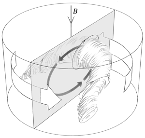
Our liquid-metal pub crawl experiment (PCE) has generated a unique set of laboratory tie points between RBC, MC, RC and RMC, while simultaneously demonstrating that robust, rapid dynamical transitions can occur in liquid-metal flows. As shown schematically in figure 6, the PCE reveals the broad variety of convective modes that arise in convecting liquid metals, including jump rope vortices (RBC and MC1), thermoelectric magnetoprecessional modes (MC1), and cohabiting bulk and wall modes (MC2, RC and RMC1). In addition, the results show the importance of sidewall and boundary transport processes in contained convective systems (cf. Net, Garcia & Sanchez Reference Net, Garcia and Sanchez2008; Lu et al. Reference Lu2021). In particular, a novel, large-amplitude magnetostrophic wall mode has been found in the RMC2 subcase. Although the bulk analogue to the RMC2 magnetostrophic wall mode purportedly dominates local-scale convection in planetary and stellar dynamo systems (King & Aurnou Reference King and Aurnou2015; Yadav et al. Reference Yadav, Gastine, Christensen, Duarte and Reiners2016), the elusive  $\varLambda \sim 1$ bulk mode has yet to be unambiguously detected in the laboratory. This necessitates future $\varepsilon _S \simeq 0$ and $\varepsilon _S \gg 0$ experimental pub crawls to determine whether bulk convection is ever strongly enhanced in the magnetostrophic regime or if other flows more efficiently drive dynamo action in planets and stars. Cheers!
Schematized flow states from the PCE. (a) JRV in the RBC subcase. (b) Thermoelectric precession of the JRV in the low-interaction-parameter ( $N \simeq 1$) magnetoconvection subcase MC1. The precession direction is set by the (downward) magnetic field orientation. (c) Quasi-stationary flow in the $N = {O}(10)$ subcase MC2, drawn following Horn & Aurnou (Reference Horn and Aurnou2019). (d) The rotating convection (RC) subcase, drawn following Horn & Schmid (Reference Horn and Schmid2017) and Favier & Knobloch (Reference Favier and Knobloch2020), features oscillating columnar bulk modes and retrograde drifting wall modes (where the rotation vector is upwards). (e) The weakly magnetic $\varLambda = 0.06$ rotating magnetoconvective subcase RMC1 has the same fundamental features as in the RC subcase. (f) The $\varLambda = 0.99$ subcase RMC2 features a stably stratified fluid bulk and magnetostrophic wall modes that drift at $\simeq$1/2 the rate found in RC, but still at 15 times the JRV's magnetoprecession rate found in MC1.

Acknowledgements
We thank three anonymous referees and K.R. Tometsko for constructive feedback that improved this document. The PCE was first performed as a live demonstration at the IPAM Mathematics of Turbulence long programme (NSF DMS 1925919), after which C.P. Caulfield suggested it might be worked into a formal publication.
Funding
This research was supported by the National Science Foundation (J.A., EAR 1620649; EAR 1853196); and the Engineering and Physical Sciences Research Council (S.H., EP/V047388/1).
Declaration of interests
The authors report no conflict of interest.
Data availability statement
The data that support the findings of this study are included within the article.


 Open access