







1. Introduction
Horizontal convection (HC) is a ubiquitous phenomenon (Hughes & Griffiths Reference Hughes and Griffiths2008), and it manifests across a variety of scales at which horizontal density inhomogeneity is present; large-scale circulations in the atmosphere, oceans and lakes (Wunsch & Ferrari Reference Wunsch and Ferrari2004; Schneider Reference Schneider2006; Verburg, Antenucci & Hecky Reference Verburg, Antenucci and Hecky2011; Wang, Huang & Xia Reference Wang, Huang and Xia2018) land/sea diurnal breezes (Walsh Reference Walsh1974; Gille et al. Reference Gille, Llewellyn, Stefan and Statom2005), heat/cool-island circulations (Lu et al. Reference Lu, Arya, Snyder and Lawson1997a,Reference Lu, Arya, Snyder and Lawsonb; Mori & Niino Reference Mori and Niino2002; Niino et al. Reference Niino, Mori, Satomura and Akiba2006), topographically and thermally driven flows in coastal waters (Monismith et al. Reference Monismith, Genin, Reidenbach, Yahel and Koseff2006; Ulloa et al. Reference Ulloa, Ramón, Doda, Wüest and Bouffard2022), radiatively driven flows in inland waters (Coates & Patterson Reference Coates and Patterson1993; Mao, Lei & Patterson Reference Mao, Lei and Patterson2009) as well as industrial casting processes (Sarris, Lekakis & Vlachos Reference Sarris, Lekakis and Vlachos2002; Gramberg, Howell & Ockendon Reference Gramberg, Howell and Ockendon2007; Chiu-Webster, Hinch & Lister Reference Chiu-Webster, Hinch and Lister2008). Motivated by such broadly existing processes, HC continues to be investigated using the conceptual model illustrated in figure 1(a) (e.g. Wang & Huang Reference Wang and Huang2005; Coman, Griffiths & Hughes Reference Coman, Griffiths and Hughes2006; ILIcak & Vallis Reference ILIcak and Vallis2012; Shishkina, Grossmann & Lohse Reference Shishkina, Grossmann and Lohse2016) since the pioneering study by Rossby (Reference Rossby1965). It is evident, however, that the traditional HC model requires additional elements to represent the complexity of actual systems, such as rotation and vertical density gradients (Couston, Nandaha & Favier Reference Couston, Nandaha and Favier2022; Gayen & Griffiths Reference Gayen and Griffiths2022).
Schematic of (a) HC with  $T_1< T_2$ and (b) stratified horizontal convection with $T_0< T_1< T_2$. Thermal boundary conditions are noted. Overturning circulations are indicated by arrows. Linear density profiles imposed only by the boundary conditions are drawn by dashed lines, and the solid lines indicate mean density profiles after convective motions.

The traditional model of HC (figure 1a) considers a closed fluid system that is thermally insulated except on one of its horizontal surfaces, where a destabilising horizontal temperature difference,  $\Delta \theta = T_2 - T_1$, is imposed. This system eventually reaches a statistical equilibrium state characterised by a basin-scale overturning circulation that penetrates the full depth of the domain and develops over the full horizontal extent. Two main dimensionless parameters govern the dynamics of this fluid system. One is the Prandtl number defined as $Pr=\nu /\kappa$, meaning the ratio of viscous diffusion to heat diffusion, where $\nu$ is the kinematic and $\kappa$ the thermal diffusivity of the fluid. The other is the Rayleigh number, $Ra = u_{s}\,W/\kappa$, that quantifies the relative strength between convective and conductive heat transport within the thermally forced fluid system, with $u_{s}$ and $W$ the characteristic velocity scale of the thermally driven flow and the horizontal length scale across which thermal forcing is exerted. Conventionally, $u_{s}$ is derived from a balance between buoyancy and viscous forces, i.e. $u_{s}=g \alpha \Delta \theta W^{2}/\nu$, where $g$ and $\alpha$ are the gravitational acceleration and the thermal expansion coefficient. The latter leads to the classic definition of the Rayleigh number
 \begin{equation} Ra = \frac{g\alpha\Delta\theta W^3}{\kappa\nu}. \end{equation}
In addition, the fluid dynamics of HC is also influenced by the aspect ratio of the fluid body, i.e.  $\mathcal {A} = W/H$ with $H$ the thickness of the fluid layer. Thus, flow features, such as the heat transport and energetics, can be characterised in terms of $Pr$,
$Pr$,  $Ra$ and $\mathcal {A}$ (Hughes & Griffiths Reference Hughes and Griffiths2008; Gayen, Griffiths & Hughes Reference Gayen, Griffiths and Hughes2014; Shishkina et al. Reference Shishkina, Grossmann and Lohse2016). In nature, however, fluid bodies experiencing surface differential heating/cooling – such as oceans, seas and lakes – hold a density stratification, unlike the idealised scenario above. Such a background stratification, usually controlled by a vertical temperature gradient, acts as a stabilising mechanism against destabilising buoyancy-driven fluid motions that enhance vertical mixing. Thus, when a fluid system is thermally stratified, the overturning circulation does not penetrate the depth of the basin, as illustrated in figure 1(b). Hereafter, we call this system stratified HC (SHC), i.e. HC of a thermally stratified fluid body driven by surface differential heating. In the case of SHC, the overturning circulation develops within the uppermost fluid region. In contrast, the cooler and deeper stratified fluid remains stable and weakly energised. Notice that the dynamic response of differential cooling at the bottom surface of a thermally stratified basin is an upside-down analogue to the above scenario: the circulation is confined to the deeper region beneath the warmer and shallower stratified fluids. Intuitively, the flow features of SHC are bonded to the strength of the background stratification, characterised, for instance, by the Richardson number $Ri$ (Peltier & Caulfield Reference Peltier and Caulfield2003), in addition to the destabilising buoyancy force ruled by $Ra$. Therefore, unlike in HC where the overturning circulation forms throughout the full depth, the presence of stratification exerts a confining effect in SHC, requiring the identification of the optimal vertical length scale characterising the thickness of the overturning circulation. Finding this vertical length scale from the prescribed parameters only is essential. To the best of our knowledge, the fundamental flow features of SHC depicted in figure 1(b) remain unknown. Therefore, the first sound step is building upon the current understanding of HC. As reported earlier (Scotti & White Reference Scotti and White2011; Gayen et al. Reference Gayen, Griffiths, Hughes and Saenz2013, Reference Gayen, Griffiths and Hughes2014; Passaggia, Scotti & White Reference Passaggia, Scotti and White2017), traditional HC can reach three-dimensional (3-D) states by increasing $Ra$. Therefore, one can expect that SHC may also experience a transition from quasi-two-dimensional (Q2-D) to 3-D flow states for specific conditions. In fact, a transition to a 3-D state has been observed in the atmosphere as formations of clouds elongated in the flow direction at land–sea/lake borders, known as horizontal convective rolls (Lemone Reference Lemone1973; Weckwerth, Wilson & Wakimoto Reference Weckwerth, Wilson and Wakimoto1996; Dailey & Fovell Reference Dailey and Fovell1999). Identifying the conditions under which such a transition occurs may provide insights into the mechanisms, energy and parameters governing the local and global fluid dynamics of SHC. Gaining this knowledge is significant for quantifying the heat and mass distributions and the ventilation of geophysical fluid environments, all critical factors influencing their ecosystem's functioning and health. Here, we shed light on the following general questions:
(i) What parameters control the dynamics of SHC?
(ii) How much fluid does SHC transport?
(iii) What flow structures can emerge in SHC?
(iv) What mechanism controls the transition from Q2-D to 3-D states?
To address these questions, we designed and performed laboratory experiments utilising a water tank subject to steady surface differential heating and uniform cooling at its bottom boundary. The manuscript is organised as follows. In § 2, we introduce the conceptual model and the characteristic dimensionless parameters. Next, in § 3, we describe the laboratory experimental set-up. Results are reported in § 4, and we focus on describing and characterising the local and global flow features, as well as the available mechanical energy. In § 5, we discuss the mechanisms governing the formation of longitudinal rolls – the signature of the three-dimensionality. Finally, we summarise our findings in § 6.
2. Characteristic scales and dimensionless parameters
Unlike the traditional HC, the characteristic scales associated with SHC are not set by the basin aspect ratio  $\mathcal {A}$. In the stratified scenario, the background density gradient must play a role in the controlling parameters and the dynamics of SHC. Yet, these scales are, a priori, unknown. Here, we derive the characteristic scales for SHC considering an Oberbeck–Boussinesq fluid with a linear equation of state, $(\rho -\rho _{0})/\rho _{0} =-\alpha (T-T_{0})$, where $\rho $ is the density of the fluid. Without loss of generality, let us consider an initially thermally stratified fluid cooled from the bottom and differentially heated at its surface boundary. This scenario leads to a baroclinic adjustment owing to the horizontal density (or buoyancy) gradient developed at the surface, which ultimately drives a horizontal overturning circulation. The degree of stratification is essential in SHC as the restoring force exerted by the background stratification may substantially limit the vertical extent of the overturning circulation. In this case, the Rayleigh number (1.1) alone does not describe the fluid dynamics, as shown by Noto et al. (Reference Noto, Terada, Yanagisawa, Miyagoshi and Tasaka2021), and an additional parameter describing the stabilising mechanism is required. Mori & Niino (Reference Mori and Niino2002) investigated the progressive evolution of HC within a semi-infinite stratified domain caused by a localised cooling at the bottom. To characterise the influence of stratification on the transient flow, the authors introduced the dimensionless parameter $\varGamma ' = (\partial T/\partial z) / (\Delta \theta / \ell )$ – instead of $Ri$. Here, $\ell = [\kappa ^2/(g\alpha \Delta \theta )]^{1/3}$ is the horizontal length scale at which the baroclinic torque is prominent. The parameter $\varGamma '$ describes the competition between the restoring effect of the background stratification and the destabilising effect of buoyancy, and it is time dependent until the system reaches an equilibrium state, as the vertical temperature gradient $\partial T/\partial z$ relaxes with time owing to thermal diffusion. Recently, Noto et al. (Reference Noto, Terada, Yanagisawa, Miyagoshi and Tasaka2021) confirmed through laboratory experiments in a closed water basin that $\varGamma '$ characterises well the flow features developed by HC confined by an underlying stratification. These studies (Mori & Niino Reference Mori and Niino2002; Noto et al. Reference Noto, Terada, Yanagisawa, Miyagoshi and Tasaka2021) have focused only on transient processes towards equilibrium states. In the equilibrium states for a laterally confined fluid body, however, this horizontal length scale $\ell$ is no longer relevant since the overturning circulation takes place over the whole horizontal extent of the system $W$. In this sense, $\varGamma '$ might help to characterise the early transient dynamics in a domain large enough such that the initial evolution of HC is not affected by the lateral boundaries. It is not straightforward to characterise the ‘effective bulk vertical temperature gradient’ in a laterally confined domain owing to the formation of the overturning circulation. Hence, in the case of closed, complex fluid environments, new characteristic scales are required to describe the fluid dynamics of SHC. In particular, for characterising the global properties of SHC, a universal dimensionless parameter should integrate bulk quantities, such as the energy available to catalyse fluid motion.
To tackle the above quest, we posit a simple question: how much energy is potentially available to sustain SHC? To address this question, we consider the available potential energy (APE) framework (Winters et al. Reference Winters, Lombard, Riley and D'Asaro1995). In a system whose fluid parcels are out of their gravitational equilibrium positions, APE quantifies the reservoir of energy that can drive motion and enhance mixing. It is defined as the excess of potential energy that a fluid system of volume  $V$ stores relative to its state of minimum or background potential energy (BPE)
 \begin{equation} E_{bp} \equiv \int_{V}g \rho z_{{\star}}\,{\rm d}V, \end{equation}
where  $z_{\star }$ denotes the equilibrium height of each fluid parcel of density $\rho$ in the system. Computing BPE requires sorting of the fluid parcels adiabatically so that each fluid element is found at its height of gravitational equilibrium. Therefore, if the gravitational potential energy (GPE) of a system is $E_{p}=\int _{V}g \rho z\,{\rm d}V$, with $z$ the height of fluid parcels relative to a coordinate reference system (conventionally defined positive upward), then APE is determined by
 \begin{equation} E_{ap} \equiv \int_{V}g\rho\left(z-z_{{\star}}\right)\,{\rm d}V. \end{equation}
The coordinate  $z_{\star }$ can be computed by utilising the adiabatic sorting method (Winters et al. Reference Winters, Lombard, Riley and D'Asaro1995) or the probability density function method (Tseng & Ferziger Reference Tseng and Ferziger2001). Although the latter is more robust, we follow the former for perceptual explicitness as described in detail by Winters & Barkan (Reference Winters and Barkan2013). Here, we summarise the key steps involved in the algorithm. First, fluid parcels are defined as discretised forms, i.e. the whole volume $V$ is divided into a number of fluid parcels with a volume of $\Delta V({\boldsymbol x})$ and a density of $\rho ({\boldsymbol x})$ at a position ${\boldsymbol x}$. Second, the fluid parcels are sorted into their gravitational equilibrium positions, such that the densest fluid parcels form the deepest layer while the least dense fluid parcels form the uppermost layer. Conceptually, this adiabatic sorting is performed instantaneously, leading to a monotonically increasing density distribution from top to bottom. Third, the original shape of the parcel is modified to fit on the horizontal area of the system while keeping $\Delta V$. That is, each fluid parcel has a height of $\Delta V/A$, where $A$ is the horizontal cross-section of the domain. The fluid volume is eventually filled up by the ‘flattened’ parcels. Thus, we can build a one-to-one relationship between the density $\rho$ of a fluid parcel at a position $\boldsymbol x$ and its equilibrium height, $z_{\star }(\boldsymbol {x})$. The latter allows us to estimate how far (in the vertical direction) a fluid parcel is from its equilibrium height. Notice that the definition range of $z_\star$ matches exactly that of $z$. Figure 2 schematises the adiabatic sorting in a fluid system subject to differential heating. Let us consider the fluid body shown in figure 2(a). Its domain has a maximum height of $H$, a horizontal length of $W$ and a thickness of $L$. The top surface is differentially heated as $T(0 \leq x < cW) = T_2$ and $T(c\,W \leq x \leq W) = T_1$, where $T_1 < T_2$. In contrast, the bottom surface is uniformly cooled at $T_{0}$ with $x\in [0,W]$. Here, $c$ is an area ratio of the differentially heated surfaces, i.e. $0 < c < 1$. For the sake of simplicity, we assume that the domain is linearly stratified only in the $z$ direction, without mixing horizontally. The vertical density profiles are drawn in figure 2(b). In this hypothetical scenario, each position $x$ has a locally (yet not global) stable density distribution such that the horizontal density difference between the extreme lateral boundaries, i.e. $x/W=0$ and $x/W=1$, increases as a function of $z/H$. After the adiabatic sorting, the original density distribution shown in figure 2(a) transforms into the rearranged density distribution illustrated in figure 2(c). This fully stable density defines the state of minimum potential energy, i.e. the BPE. Note that density at an arbitrary horizontal slice, $\rho (x,y)$, for the background state, is constant. Thus, the APE and the BPE can be readily computed through the one-to-one relationship, $z_\star (\rho )$, illustrated in figure 2(d); the APE stored in the system results by subtracting the BPE distribution (figure 2c) from the GPE distribution (figure 2a).
Schematic of adiabatic sorting: (a) linear stable stratification, (b) vertical density profiles at  $x=0$ and $W$, (c) minimum energy (background) state after adiabatic sorting (d) $z_\star (\rho )$.

Here, we use the concepts of an equilibrium height and APE to characterise the physical length scales and dimensionless parameters governing SHC. In particular, we seek to find a characteristic length scale of the system,  $h$, associated with the vertical excursion that fluid parcels with density $\rho _1$ perform to reach their equilibrium height $h_{\star }$ via the overturning circulation. In this case, the length scale can be obtained without sorting. After the adiabatic rearrangement, the fluid volume having a temperature lower than $T_1=T_0+\Delta T$ should be $W h_\star L$. This volume is identical to the sum of the fluid volume having a temperature lower than $T_1$ in the linearly stratified system before the sorting. Considering heights of fluid parcels having temperatures of $T_1$ as $H_1$ and $H_2$ in the right and left regions, respectively, the corresponding fluid volumes are easily computed as
 \begin{equation} V_1 = W_1 H_1 L = (1-c)W H L, \end{equation}
and
 \begin{equation} V_2 = W_2 H_2 L = c W \left(\frac{\Delta T}{\Delta T + \Delta \theta}\right) H L = c W \left(\frac{1}{1 + \varTheta}\right) H L. \end{equation}
Here,  $\varTheta$ is the ratio of the temperature differences $\varTheta = \Delta \theta / \Delta T$. Considering mass conservation during the sorting, we obtain the following relationship:
 \begin{equation} W h_\star L = (1-c)W H L + c W \left(\frac{1}{1 + \varTheta}\right) H L. \end{equation}
Equation (2.5) yields a determination of the equilibrium height  $h_\star$ as
 \begin{equation} h_\star = \left[\frac{1 + (1-c) \varTheta}{1 + \varTheta}\right]H. \end{equation}
Accordingly, fluid parcels initially at  $H_1$ in the right region are displaced by $h_1 = H_1 - h_\star$. Likewise, those parcels initially at $H_2$ in the left region are displaced by $h_2 = h_\star - H_2$. To globally define $h$, these displacements are laterally averaged, giving
 \begin{equation} h = (1-c)h_1 + c h_2 = 2c(1-c)\left(\frac{\varTheta}{1 + \varTheta}\right)H. \end{equation}
The displacement  $h$ is a fundamental length scale of SHC and can be determined solely from prescribed parameters while considering the horizontal temperature gradient $\Delta \theta$ as a driving force and the vertical temperature difference $\Delta T$ as a braking force. Notice that $h$ is maximised at $c=1/2$. Here, however, $c$ is fixed at $0.25$ for all the conditions examined in this study, as explained later. The value of $h$ can be derived irrespective of the thermal boundary conditions as long as the temperatures are prescribed – for instance, a linear horizontal temperature gradient (Rossby Reference Rossby1965) and more complex cases. Let us now assume that all the APE in the system is converted into the kinetic energy (KE) of the overturning circulation, i.e.
 \begin{equation} E_{ap} \sim E_{k}. \end{equation}
In the Oberbeck–Boussinesq limit, KE is defined as
 \begin{equation} E_{k} \equiv \frac{\rho_0}{2}\int_{V}|{\boldsymbol u}|^2\,{\rm d}V. \end{equation}
The relationship (2.8) allows linking of the characteristic length  $h$ and density anomaly characterising the APE with the advection velocity scale $U_{adv}$ associated with the KE as
 \begin{equation} g\Delta\rho h \sim \rho_0U_{adv}^2, \end{equation}
where  $\Delta \rho$ is the density difference of the fluid corresponding to the temperature difference of $\Delta \theta$, i.e. $\Delta \rho = \rho _0\alpha \Delta \theta$. The velocity scale is thus derived as
 \begin{equation} U_{adv} = \left(g\alpha\Delta\theta h\right)^{1/2}. \end{equation}
If we consider the magnitude of the controlling parameters at the laboratory scale,  $U_{adv}$ is typically in the range $O(10^0$– $10^1\,{\rm mm}\,{\rm s}^{-1})$ which agrees well with the observed maximum values in experiments. Thus, $U_{adv}$ is a reasonable velocity scale for the SHC problem. We now define the bulk Richardson number $Ri$ – the ratio of the stratified fluid stability to the shear driven by the overturning circulation – to represent the strength of the background stratification. Using the square of the buoyancy frequency $N^2 = g\alpha \Delta T / H$ and the characteristic shear rate of the system $S = U_{adv}/H$, we can estimate, a priori, the bulk Richardson number from the prescribed parameter of the problem as
 \begin{equation} Ri \equiv \frac{N^2}{S^2} = \frac{g\alpha\Delta T/H}{(U_{adv}/H)^{2}} = \frac{1}{\varTheta}\frac{H}{h}=\frac{1 + \varTheta}{2c(1-c)\varTheta^2}. \end{equation}
Finally, we consider the Péclet number  $Pe$ – the ratio of convective heat transport to heat diffusion – as an optimal dimensionless parameter to diagnose the local and global dynamics of SHC. Here, we assume the system to be in a dynamic regime in which transport is dominated by convection. Therefore, using the velocity scale $U_{adv}$ (2.11), $Pe$ is defined as
 \begin{equation} Pe \equiv \frac{U_{adv} W}{\kappa} = \frac{\left(g \alpha\Delta \theta h\right)^{1/2} W}{\kappa} = \left(\frac{Pr\, Ra}{\mathcal{A}\, Ri\, \varTheta}\right)^{1/2} . \end{equation}
Remarkably,  $Pe$ integrates all the dimensionless parameters introduced so far and is obtained only using the prescribed parameters of the system. That is, $Pe$ comes forward as an intrinsic parameter to the global characteristics of SHC ahead of $Ra$ and $Ri$.
$Ri$.
3. Laboratory experiments
Laboratory experiments were performed using a rectangular acrylic fluid container, similar to that recently developed in Noto et al. (Reference Noto, Terada, Yanagisawa, Miyagoshi and Tasaka2021) and Terada et al. (Reference Terada, Noto, Tasaka, Miyagoshi and Yanagisawa2023) to study thermally driven HC in stratified fluids; see schematic in figure 3(a). The basin-scale dimensions of the fluid body are  $W=200$ mm, $L=50$ mm and $H=100$ mm in the $x$–
$x$– $y$–
$y$– $z$ directions, respectively. Accordingly, the aspect ratio is $\mathcal {A} = 2$. The experimental fluid is distilled water, with characteristic Prandtl number $Pr\approx 7$ at $20\,^{\circ }{\rm C}$.
Schematics of experimental set-up: (a) front view showing the temperature conditions and (b) top view showing the optical configurations. Units are in mm.

Four independent heating/cooling units imposed thermal boundary conditions on the top and bottom. Each unit is formed by a copper plate whose inward-looking surface is in direct contact with the experimental fluid, whereas its outward-looking surface is bathed by temperature-controlled water. We can thus control the fluid temperature in contact with the inward-looking copper surface. In the present study, we set a ‘uniform temperature’ on the bottom, i.e. the four units have the same temperature,  $T=T_{0}>T_{md}\approx 4^{\circ }{\rm C}$, with $T_{md}$ the temperature of maximum density. In contrast, the top units are differentially heated. The first three units (from right to left) were set to be at $T=T_{1}=T_{0}+\Delta T$, and they heat three quarters of the top surface, $3WL/4$. On the other hand, the fourth unit was set to be at $T=T_{2}=T_{1}+\Delta \theta$ and heats the rest quarter of the total surface area, $WL/4$. To ensure a steep horizontal temperature gradient, we used a 4 mm thick rubber sheet to isolate the upper chambers from each other, as shown in figure 3(a). The horizontally asymmetric top temperature distribution is chosen to ensure a long-enough downstream region to develop the fluid motion after the steepest horizontal temperature gradient at $x\approx c\,W$, with $c=1/4$. Since the rubber sheets are sandwiched by the neighbouring heating units, the temperature between the heating units varies linearly. Thus, as shown by Noto et al. (Reference Noto, Terada, Yanagisawa, Miyagoshi and Tasaka2021), the top surface temperature distribution can be modelled as
 \begin{equation} T(x,y, z=H) = T_{top}(x,y) = \underbrace{T_0 + \Delta T}_{T_1} + \frac{\Delta\theta}{2} \left\{\tanh{\left[-\frac{2(x-c\,W)}{d}\right]} + 1\right\}, \end{equation}
where  $d$ is the characteristic horizontal length between $T_{2}$ and $T_{1}$. Here, we consider that the vertical temperature difference $\Delta T$ and the horizontal temperature difference $\Delta \theta$ are always positive. Under this scenario, SHC requires the following relationship:
 \begin{equation} T_{md} < T_0 < T_1 < T_2. \end{equation}
Notice that SHC also emerges for ‘surface cooling’ cases, when  $T_{ice} < T_2 < T_1 < T_0 < T_{md}$, where $T_{ice}$ is the freezing temperature $T_{ice}=0\,^\circ {\rm C}$ under atmospheric pressure. The above temperature relationships yield that the fluid lying beneath the overturning circulation is always stably stratified. In this study, we examined three different stratifications of varying strength, $\Delta T = 0.2$, $1$,
$1$,  $10\,{\rm K}$, with varying $\Delta \theta$. Table 1 summarises the parameter space of the experiments.
Experimental conditions using water ( $Pr \approx 7$) as the test fluid.

We measured the velocity field via particle image velocimetry (PIV). For this, we seeded particles encapsulated thermochromic liquid crystals (TLC) into the fluid as tracers. Thanks to their material properties and high traceability (mean diameter of  $\sim 20\,\mathrm {\mu }{\rm m}$ and specific gravity of $1.01$), TLC particles allow for robust PIV measurements. We emphasise that, although TLC particles enable visualising of the fluid temperature when excited by white light (Noto et al. Reference Noto, Tasaka, Yanagisawa and Murai2019; Anders et al. Reference Anders, Noto, Tasaka and Eckert2020), we did not use them for that purpose. The set-up of the optical configuration is shown in figure 3(b). We captured images in two ways to resolve the velocity fields in different planes to thus investigate their three-dimensionality. Firstly, we visualised the $x$–
$x$– $z$ plane at $y = 0.5L$ (the centre of the fluid layer) using a green laser sheet and camera A, as illustrated in figure 3(b). This optical configuration enables measuring of the velocity field of the primary overturning circulation driven by the surface horizontal temperature gradient with a spatial resolution of 1 mm. Secondly, we visualised ten $y$–
$y$– $z$ planes across the $x$ axis, from $x = 0.05W$ to $x = 0.95W$, every $0.10W$ interval. In this case, we used a halogen light sheet and camera B, as shown in figure 3(b). An actuator, controlled by a micro-computer, allowed the positioning of the halogen light sheet at the various measurement positions along the $x$ axis. The two lighting systems were synchronised such that only one of them was on (and off) at a time. The ten planes were visualised in about 1 min. Thus, an entire measuring loop of the $x$–
$x$– $z$ plane and the ten $y$–
$y$– $z$ planes took approximately 1.5 min.
In the beginning, the fluid was at rest and uniformly stratified,  $T(t=0,x,y,z=0)=T_0$ and $T(t=0,x,y,z=H)=T_1$. Achieving the stable thermal stratification took typically $\sim 2$ h. Once the fluid was stratified, we imposed a horizontal (surface) temperature difference $\Delta \theta$ and started to perform quasi-instantaneous measurements every 20 min to track the fluid dynamics of SHC. Initially, the flow experienced a transient regime, yet, it reached a quasi-steady state after 1 h, irrespective of the experimental parameters. In the following, we only report and analyse the results observed after 2 h of starting the surface differential heating.
4. Results
4.1. Flow structures
We first examine the characteristic fluid dynamics of SHC. Figure 4 illustrates experimental results from two thermal forcing conditions. The top panels show the flow features in a strongly stratified environment,  $Ri = 5.33$. In contrast, the bottom panels show flow features for a weakly stratified environment, $Ri = 0.14$. The left panels highlight the velocity field of the basin-scale overturning circulation on the $x$–
$x$– $z$ plane at $y=0.5L$. The circulation is clockwise due to the baroclinic adjustment experienced between the warmer and the colder surface waters. The effect of stratification in the active layer where SHC takes place is striking. In a strongly stratified environment, SHC is vertically confined to a thin region near the surface, $z/H \gtrsim 0.8$, and its velocity field is predominantly horizontal. Whereas, in a weakly stratified environment, SHC covers almost half of the water column, $z/H \gtrsim 0.5$, and its velocity field can reach large vertical magnitudes. In all of the experiments, the active layer has an upper downstream region of the overturning circulation that is thinner and moves faster than the thicker lower upstream region. Beneath the active layer, the fluid is essentially quiescent and decoupled from the SHC. These flow structures are quasi-steady irrespective of the forcing conditions. Additionally, the centre and right panels in figure 4 show the normalised vorticity component in the streamwise (i.e. $x$) direction, $\omega _{x}/|\omega _{y}|_{max}$ at two locations along the main axis. Here, $\omega _{x}$ is normalised by the maximum spanwise vorticity magnitude $|\omega _{y}|_{max}$ in order to compare the strength of the secondary flows with the main circulations. The centre panels show $\omega _{x}/|\omega _{y}|_{max}$ at $x=0.25W$, where the maximum horizontal temperature gradient is imposed. In the region $0 \leq x/W \leq 0.25$, the active layer does not exhibit vorticity, and the largest but still small magnitudes are observed near the vertical walls. The right panels show $\omega _{x}/|\omega _{y}|_{max}$ at $x=0.65W$; here, the vorticity field has a distinctive signature, especially for those cases with weak stratification. However, for systems hosting strong stratifications, the vorticity magnitude is substantially weaker, less than 10 %, suggesting that SHC is practically two-dimensional in those cases. Regardless of the strength of the background stratification, the largest magnitudes of $\omega _{x}/|\omega _{y}|_{max}$ are found in the region $0.25 < x/W \leq 1$. In this zone, the warmer fluid transported from the upper left region $0 < x/W \leq 0.25$ gets exposed to the cooler top surface. This leads to an unstable density distribution within the upper downstream region of the overturning circulation, which fosters the development of Rayleigh–Bénard rolls in the $y$–
$y$– $z$ planes and vorticity production. Such a coherent vortical pattern is not identified in strongly stratified cases, suggesting that SHC can transition from Q2-D to 3-D regimes depending on the forcing conditions.
Flow fields measured by PIV for different conditions: (a) a strongly stratified case  $Pe = 2.8\times 10^4$ and $Ri = 5.33$ ( $\Delta T = 10\,{\rm K}$ and $\Delta \theta = 10\,{\rm K}$), and (b) a weakly stratified case $Pe = 5.4\times 10^4$ and $Ri = 0.14$ ( $\Delta T = 1\,{\rm K}$ and $\Delta \theta = 20\,{\rm K}$). Panels (a i,b i) show the $x$–
$x$– $z$ planes at $y=0.5L$ with a contour of in-plane velocity magnitude $\sqrt {u^2 + w^2}$. Panels (a ii,b ii) and (a iii,b iii) show the $y$–
$y$– $z$ planes at $x=0.25W$ and $0.65W$ with contours of the streamwise vorticity fields $\omega _x$. The in-plane velocity magnitude is normalised by the maximum value $U_{max}$ and the streamwise vorticity is normalised by the maximum of the absolute spanwise vorticity $|\omega _y|_{max}$. The reverse triangles in the panels (a i,b i) correspond to the positions of $y$–
$y$– $z$ planes displayed in (a ii,b ii) and (a iii,b iii). Velocity vectors shown here are reduced from the original resolution for visibility.

We examine the three-dimensionality of the flow state shown in figure 4(b) by reconstructing the spatial structure of the streamwise vorticity component,  $\omega _{x}$. For this, we used the PIV measurements made in the $y$–
$y$– $z$ plane every $0.1W$, between $x=0.05W$ and $x=0.95W$. Here, $\omega _{x}$ was interpolated between two consecutive planes for display. Figure 5 illustrates isosurfaces of $\omega _x/|\omega _{y}|_{max}$ for two experiments within the upper active layer, $0.8\leq z/H\leq 1$. Both experiments have similar Péclet numbers, $Pe = 5.4 \times 10^{4}$ and $5.5 \times 10^{4}$, yet different $Ri$. Results in panels (a) and (b) are characterised by $Ri = 0.14$ and $0.027$, respectively. Notice that figure 5(a) corresponds to the case shown in figure 4(b). In both cases, $\omega _{x}$ emerges from the zone that hosts the maximum horizontal temperature gradient, i.e. $x/W \approx 0.25$. However, around $x/W \approx 0.3$– $0.4$, the streamwise vorticity reveals the existence of coherent longitudinal roll structures (LRSs) that self-organise over the entire spanwise domain until the end of the basin, $x/W=1$. The self-organisation of LRS is complex, however. Figure 5 shows that once LRSs form, their wavenumber decreases downstream due to the coalescence of adjacent rolls. The latter process is evident when comparing the number of roles at $x/W=0.5$ and $x/W=0.95$. In particular, we identify that the wavenumber attributed to LRS is bigger for the case with the weaker stratification, figure 5(b), than the scenario with the stronger stratification, figure 5(a). It is worth noting that LRS has significantly weaker vorticity than SHC. Indeed, the strength of LRS vorticity is approximately 10 % of that in the basin-scale overturning circulation at the most. Although earlier studies on traditional HC have reported the emergence of LRS (Mullarney, Griffiths & Hughes Reference Mullarney, Griffiths and Hughes2004; Gayen et al. Reference Gayen, Griffiths and Hughes2014; Vila et al. Reference Vila, Discetti, Carlomagno, Astarita and Ianiro2016), their emergence and evolution in stratified environments have not been investigated in detail yet.
Isosurfaces of streamwise vorticity  $\omega _x$ for the case of a 3-D flow state realised with the same $\Delta \theta$.(a) The intermediate stratification case, $Pe = 5.4\times 10^4$ and $Ri = 0.14$ ( $\Delta T = 1\,{\rm K}$ and $\Delta \theta = 20\,{\rm K}$). (b) The weak stratification case, $Pe = 5.5\times 10^4$ and $Ri = 0.027$ ( $\Delta T = 0.2\,{\rm K}$ and $\Delta \theta = 20\,{\rm K}$).

4.2. Fluid transport and flow regimes
The basin-scale fluid transport can be characterised by means of the streamfunction,  $\psi$, that satisfies the Poisson equation
 \begin{equation} \nabla^2 \psi = \omega_{y},\quad {\rm with} \ \psi=0 \quad \text{at the boundaries}. \end{equation}
We integrated (4.1) to resolve  $\psi$ using the successive over-relaxation method, as previously done in Noto et al. (Reference Noto, Terada, Yanagisawa, Miyagoshi and Tasaka2021). Here, we investigate the global transport properties of SHC by mapping $\psi _{max}$ against dimensionless parameters introduced in § 2. Figure 6 displays the maximum streamfunction $\psi _{max}$ normalised by the thermal diffusivity $\kappa$ vs $Ra$,
$Ra$,  $Ri$ and $Pe$, respectively. Solid lines indicate power-law trends, $\psi _{max} \propto Ra^{1/2}$, $\propto Ri^{-1/2}$ and $\propto Pe$.
Maximum streamfunction  $\psi _{max}$ plotted for (a) $Ra$, (b) $Ri$ and (c) $Pe$. Solid lines represent power-law trends.

As shown in figure 6(a),  $\psi _{max}$ increases with $Ra$, meaning that a stronger horizontal destabilising effect transports more fluid. In the case of HC, i.e. with no stable background stratification, the maximum streamfunction $\psi _{max}$ has been found to fulfil the well-known theoretical scaling $\psi _{max} \propto Ra^{1/5}$ (e.g. Rossby Reference Rossby1965; Hughes & Griffiths Reference Hughes and Griffiths2008; Shishkina et al. Reference Shishkina, Grossmann and Lohse2016). The power-law trend of $Ra$ for SHC seems stronger, as indicated by the solid line, $\psi _{max} \propto Ra^{1/2}$. There is, however, an evident deviation among experiments owing to different background stratifications, making $Ra$ unsuitable for describing the transport associated with SHC. In contrast to the trend on $Ra$,
$Ra$,  $\psi _{max}$ decreases as $Ri$ increases, as shown in figure 6(b). This trend, $\psi _{max} \propto Ri^{-1/2}$, highlights that the strength of the overturning circulation is substantially controlled by the strength of background stratification, i.e. the stratification suppresses the convective motions. Similarly to $Ra$, however, $Ri$ does not provide a unifying trend. This trend is similar to the previously obtained experimental scaling $\psi _{max} \propto \varGamma '^{-1/2}$ found by Noto et al. (Reference Noto, Terada, Yanagisawa, Miyagoshi and Tasaka2021), even though it was obtained for transient processes. Since the same scaling was found in different configurations, $Ri$ defined in this study can be regarded as an analogue of $\varGamma '$ defined for time-dependent differential heating of cold water bodies. Figure 6(c) illustrates a striking collapse, i.e.
 \begin{equation} \psi_{max} \propto Pe. \end{equation}
In fact, the best power-law fit is  $\psi _{max} \propto Pe^{1.02 \pm 0.04}$. Note that the experimental results collapse to the scaling law (4.2) regardless of the flow dimensionality and the background stratification condition. Summing up, figure 6 shows that SHC transport is exceptionally characterised by $Pe$.
$Pe$.
Assuming  $\partial ^2/\partial x^2 \ll \partial ^2/\partial z^2$ in (4.1) for the boundary layer on the surface whose thickness is $\delta _{\nu } \ll W$, we get the following relationship:
 \begin{equation} \frac{\psi}{\delta_{\nu}^2} \sim \frac{w_{c}}{W} + \frac{u_{c}}{\delta_{\nu}}, \end{equation}
where  $u_{c}$ and $w_{c}$ are the characteristic horizontal and vertical velocities. From the continuity, $w_{c}$ is negligible as $w_{c} \sim (\delta _{\nu }/W)u_{c}$. Replacing $u_{c}$ by $U_{adv}$, we obtain
 \begin{equation} \frac{\psi}{\kappa} \sim \frac{U_{adv} \delta_{\nu}}{\kappa} = \frac{\delta_{\nu}}{W}Pe. \end{equation}
Here,  $\delta _{\nu }$ is considered as a depth of the maximum horizontal velocity from the surface and may vary with $Ra$ as in HC (Hughes & Griffiths Reference Hughes and Griffiths2008). However, we confirmed that $\delta _\nu$ does not change much with the control parameters, and typically $\delta _\nu \sim 0.03H$. Thus, the maximum streamfunction can be scaled as $\psi _{max} \propto Pe^1$.
As discussed earlier, SHC exhibits two characteristic flow regimes: (i) a Q2-D overturning circulation and (ii) an overturning circulation coupled with LRSs that make the SHC fluid dynamics three-dimensional. Figure 7(a) summarises the flow regimes for the experimental conditions investigated in this study as a function of the vertical temperature difference,  $\Delta T$ (vertical axis), the horizontal temperature difference, $\Delta \theta$ (horizontal axis) and $Pe$ in the colour map. Green circles denote experiments with a Q2-D flow state, whereas violet diamonds denote experiments with a 3-D flow state. Recall that vertical and horizontal temperature gradients characterise stabilising and destabilising forcing mechanisms, respectively. Thus, from low to high horizontal temperature differences, we expect the buoyancy-driven flow to intensify and transition from 2-D to 3-D regimes fostering HC and RBC in the uppermost zone of the fluid body. In contrast, from low to high vertical temperature differences, we anticipate a reinforcement of stratification that counteracts vertical motions, resulting in a shift from a 3-D to a 2-D flow regime. This intuitive flow behaviour is actually observed in figure 7. Furthermore, since $Pe \propto Ra^{1/2}(Ri\,\varTheta )^{-1/2}$ (see (2.13)), we can map the flow regimes into the $Ra$–
$Ra$– $Ri\,\varTheta$ space. Figure 7(b) shows that this parameter space successfully segregates the flow regimes. Empirically, it is possible to identify a border between the two flow regimes, shown by the dashed lines in figure 7. These lines characterise a unique critical Péclet number value, estimated as $Pe_{c} \approx 3.3 \times 10^4$, that allows describing of the flow dimensionality for SHC.
Regime diagram of SHC plotted for (a) the two controllable temperature differences,  $\Delta \theta$ and $\Delta T$ and (b) the two dimensionless parameters, $Ra$ and $Ri\varTheta$, for $Pr\approx 7$. Colour contour represents the Péclet number $Pe$. Dashed line, $Pe = 3.3\times 10^4$, is the estimated border for the two different flow regimes.

4.3. Available mechanical energy
Examining the energy distribution in SHC is relevant to understanding how the controlling parameters are tied to the production of available mechanical energy in the system. The system is forced only by the surface heating at a prescribed degree, and part of the created APE  $E_{ap}$ is transformed into KE $E_{k}$, in the form of convective motions (Winters et al. Reference Winters, Lombard, Riley and D'Asaro1995; Winters & Barkan Reference Winters and Barkan2013). The parameter $E_{ap}$ requires density distributions for computation, and these are hard to directly measure from experiments. Accordingly, we apply the temperature reconstruction method recently introduced in Noto, Ulloa & Letelier (Reference Noto, Ulloa and Letelier2023), which is applicable to quasi-steady thermally driven flows under well-defined boundary conditions. Density and temperature distributions are estimated from the velocity fields by solving the heat equation
 \begin{equation} \frac{\partial T}{\partial t} + {\boldsymbol u} \boldsymbol{{\cdot}} \boldsymbol{\nabla} T = \kappa \nabla^2 T. \end{equation}
Once the system reaches an equilibrium state (after approximately 2 h from imposing  $\Delta \theta$), heat advection balances heat diffusion. Although SHC supports local 3-D features for specific $Pe$ numbers, the global overturning circulation remains two-dimensional, regardless of the $Pe$ conditions. In this regard, a mean temperature field in the $x$–
$x$– $z$ plane can be reconstructed utilising PIV velocity field measurements and the steady state heat equation
 \begin{equation} u\frac{\partial T}{\partial x} + w \frac{\partial T}{\partial z} = \kappa \left(\frac{\partial^2 T}{\partial x^2} + \frac{\partial^2 T}{\partial z^2}\right). \end{equation}
The assumption of Q2-D flow is reasonable because the velocity component  $v$ in the $y$-direction is significantly smaller than those of the $x$ and $z$ components. To obtain a steady solution of $T$, we use the Dirichlet boundary conditions for the top and the bottom, and Neumann boundary conditions for the sidewalls, i.e.
 \begin{align}
T(x, z=0) = T_0,\quad T(x, z=H) &= T_{top},\nonumber\\
\text{and}\quad \left.\frac{\partial T}{\partial x}\right|_{x=0} &=
\left.\frac{\partial T}{\partial x}\right|_{x=W} =
0, \end{align}
\begin{align}
T(x, z=0) = T_0,\quad T(x, z=H) &= T_{top},\nonumber\\
\text{and}\quad \left.\frac{\partial T}{\partial x}\right|_{x=0} &=
\left.\frac{\partial T}{\partial x}\right|_{x=W} =
0, \end{align}
as temperature boundary conditions. Here, the surface temperature distribution  $T_{top}$ is estimated from (3.1). Since the heat leakage through the lateral wall estimated by the material properties is $\lesssim 4\,\%$ for the worst case, the adiabatic thermal boundary condition is reasonable. For the velocity field, no-slip conditions are imposed for all of the rigid boundaries, i.e. ${\boldsymbol u}({\boldsymbol x} \in \partial V) = {\boldsymbol 0}$. Equation (4.6) is discretised by the second-order central-difference scheme, and $T$ is obtained throughout iterative processes of the Gauss–Seidel method. Owing to the assumption of Q2-D flow, the estimated temperature fields should be slightly different from the actual one, in particular for the 3-D flows. It, however, provides reasonable estimations of temperature distributions in the proximity of the top surface, as the magnitude of $v$ is significantly smaller than those of $u$ and $w$. Once $T$ is computed, density distribution $\rho$ is obtained from a linear equation of state, $\rho = \rho _0[1 - \alpha (T - T_0)]$. As explained in § 2, the potential energy (PE) $E_{p}$ of the system can be decomposed into BPE $E_{bp}$ and APE $E_{ap}$, i.e. $E_{p} = E_{bp} + E_{ap}$. The BPE does not contribute to driving fluid motions but constantly restratifies the system; the BPE density $\mathscr {E}_{bp}$ is defined as
 \begin{equation} \mathscr{E}_{bp} = g \rho z_\star. \end{equation}
The APE, in contrast, is the energy available for fuelling SHC and enhancing mixing in the active layer. The APE density  $\mathscr {E}_{ap}$ is defined as
 \begin{equation} \mathscr{E}_{ap} = g (\rho - \bar{\rho}) (z - z_\star). \end{equation}
Here,  $\bar {\rho }$ corresponds to the compensatory displacements that emerge during the adiabatic sorting, and it is written as
 \begin{equation} \bar{\rho} = \frac{1}{z-z_\star}\int_{z_\star}^{z}\rho(\hat{z}_\star) \,{\rm d}\hat{z}_\star, \end{equation}
and accordingly,
 \begin{equation} \mathscr{E}_{ap} = g \rho (z - z_\star) - g\int_{z_\star}^{z}\rho(\hat{z}_\star) \,{\rm d}\hat{z}_\star \geq 0. \end{equation}
Notice that  $\mathscr {E}_{ap}$ is positive definite, and the second term of the right-hand side can be cancelled out by integration of the whole domain (Winters & Barkan Reference Winters and Barkan2013). The APE is thus computed by integrating $\mathscr {E}_{ap}$ for the whole domain as $E_{ap} = \int _V \mathscr {E}_{ap} \,{\rm d}V$. Considering the depth of the main overturning circulation, $h$, a scale of APE can be estimated for the limited volume $V' = (h/H)V$ as
 \begin{equation} E_{ap} \sim g\Delta\rho h V' \sim g\rho_0\alpha\Delta\theta h \left(\frac{h}{H}V\right) \propto Pe^2. \end{equation}
For the present study,  $E_{ap}$ is estimated to be $O(10^{-6}$– $10^{-4}\,{\rm J})$. The KE density, $\mathscr {E}_{k}$, is defined for each fluid parcel as
 \begin{equation} \mathscr{E}_{k} = \frac{1}{2}\rho_0|{\boldsymbol u}|^2 = \frac{1}{2}\rho_0\left(u^2 + v^2 + w^2\right), \end{equation}
where  $\rho _0$ is the reference density corresponding to the bottom temperature $T_0$. In contrast to $\mathscr {E}_{ap}$, $\mathscr {E}_{k}$ is straightforward to compute as the PIV measurements allow reconstructing of full velocity fields in the 3-D domain. To obtain the global KE, $\mathscr {E}_{k}$ is integrated over the whole domain as $E_{k} = \int _V \mathscr {E}_{k} \,{\rm d}V$. In non-SHC systems, $E_{k}$ is typically two orders of magnitude smaller than $E_{ap}$ (Gayen et al. Reference Gayen, Griffiths, Hughes and Saenz2013), meaning that only a few per cent of the APE is transformed into KE to drive the horizontal overturning circulation. Figure 8 shows the spatial distributions of the streamfunction $\psi$, the temperature $T$, the KE density $\mathscr {E}_{k}$ and the APE density $\mathscr {E}_{ap}$ for the case of Q2-D state, $Pe = 2.8\times 10^4$ and $Ri=5.33$. The results show the existence of two basin-scale overturning cells. One is localised immediately beneath the heating surface, whereas the second cell is found directly under the shallower overturning, as shown in figure 8(a). The temperature distribution in figure 8(b) shows that the system is mostly stably stratified, except for the region hosting the most vigorous circulation (see the bending of the isotherm between $x/W\in [0.25,0.5]$). As expected, figure 8(c) shows that $\mathscr {E}_{k}$ peaks within the main overturning circulation, whereas the deep stratified region remains motionless. Consistently, $\mathscr {E}_{ap}$ reaches a maximum in the shallow region, as shown in figure 8(d). We stress that the velocity component in the $y$ direction is also taken into account for computing $\mathscr {E}_{k}$, yet its contribution is less than 3 % at the maximum. This result shows that APE is mostly spent in stratifying the system and mixing the uppermost waters, whereas only the shallow region confined immediately beneath the heating surface is kinetically energised.
Spatial distributions of (a) streamfunction  $\psi$, (b) temperature $T$ estimated by (4.6), (c) KE $\mathscr {E}_{k}$ and (d) APE $\mathscr {E}_{ap}$ for the case of $Pe = 2.8\times 10^4$ and $Ri=5.33$ (Q2-D state, corresponding to figure 4a). Dashed lines indicate the theoretical estimation of the overturning circulation thickness, $z = H - h$.

Figure 9(a,b) shows the available mechanical energy components, APE and KE, vs  $Pe$. The APE has an interesting behaviour in terms of $Pe$. For a Péclet number bigger than $Pe\approx 3\times 10^{4}$, the APE follows the anticipated scaling (4.12) as $E_{ap}\sim Pe^{2}$. In contrast, for $Pe \lesssim 3\times 10^{4}$, $E_{ap}$ is less dependent on $Pe$. An intriguing aspect is that the evident break occurs exactly at $Pe\approx 3.3\times 10^{4}$, the empirical critical Péclet number at which a shift from Q2-D to 3-D flow occurs, shown in figure 7. In other words, our results suggest that the APE has a low- $Pe$ trend linked to a Q2-D SHC and a high- $Pe$ trend ( $E_{ap}\sim Pe^{2}$) associated with a 3-D SHC. Conversely, KE collapses into the line of $\sim Pe^2$. Certainly, SHC at high- $Pe$ behaves more ‘inviscid’, meaning that the theoretical scalings for KE and APE are well captured by the advective velocity scale $U_{adv}$ (2.11) and the length scale $h$ (2.7) characterising an adiabatic sorting of mass in the system.
Mechanical energies plotted for  $Pe$: (a) APE $E_{ap}$ and (b) KE $E_{k}$.

We stress that the computed KE is two orders of magnitude smaller than the APE, irrespective of  $Pe$ values. Thus, our results show that the overturning circulation is driven only by a small part of the APE. Since the system reaches a quasi-steady state, this implies that the remainder of the APE is transformed into BPE and used to sustain the stratification via irreversible thermal diffusion. This result agrees with the energy partitioning found by Gayen et al. (Reference Gayen, Griffiths, Hughes and Saenz2013) in HC, i.e. a small fraction of APE, less than 10 %, is allocated to KE.
5. Discussion
The results shown in § 4 display similarities to and differences from those in HC. To understand the fluid dynamics of SHC further, we now focus on discussing the details of the transitional flow features, LRSs and mechanical energy conversion. Since SHC posits different vertical length scales, an overall view of the flow structures is illustrated in figure 10 to clarify their relationship. The SHC exhibits structure layering from top to bottom, i.e. an overturning circulation, a secondary flow which circulates inversely to the primary circulation due to viscous coupling and a stably stratified stagnant region at the bottom. Here, we recall three length scales:  $h$, the intrinsic vertical length scale of SHC, representing the overturning circulation depth; $\delta _\nu$, the thickness associated with the viscous boundary layer at the surface and comparable to the thermal boundary layer thickness $\delta _{t}$; $\delta _{s}$, the thickness of the downstream region, explained later.
Overall view of flow structures and associated length scales.

5.1. Longitudinal roll structures
As demonstrated in § 4.1,  $Pe$, the ratio of heat transport carried by convection to that owing to thermal conduction, describes well the flow features and the flow states of SHC. Therefore, we can hypothesise that 3-D flows resulting from the emergence of LRS occur when SHC cannot fully remove the heat from the highest temperature surface. Thus, a secondary flow transports heat vertically in addition to the overturning circulation. In other words, the formation of the longitudinal rolls may result from the need for extra vertical heat transport. Here, we investigate the flow structure of longitudinal rolls and their forming mechanism immediately beneath the heating surface. Vertical profiles of horizontal velocity $u$, temperature $T$, and mean absolute streamwise vorticity $\langle |\omega _x| \rangle _y$ close to the heating surface, $z/H \geq 0.8$, at the different $x$ positions are shown in figures 11(a), 11(b) and 11(c), respectively. Here, $u$ is measured directly by PIV and normalised by the bulk maximum horizontal velocity $u_{max}$. The temperature $T$ is estimated from (4.6) using the velocity field measured by PIV and normalised by the local maximum $T_{lmax}$ at each $x$ position. The streamwise vorticity $\omega _x$ is computed from PIV, and its mean absolute value is derived by taking the spanwise average as $\langle |\omega _x| \rangle _y(z) = ({1}/{L})\int _0^L |\omega _x|(y,z) \,{\rm d}y$ at each $x$ position and normalised by the maximum absolute spanwise vorticity $|\omega _y|_{max}$. Figure 11(a) highlights in light blue the shallow streaming regions at which $u>0$. The thickness of the shallow region is expressed as $\delta _{s}$, and dashed lines indicate the zero-crossing heights of $u$. Similarly, figure 11(b) highlights in light red the regions of unstable temperature distribution $\partial T/\partial z < 0$. The unstable layer thickness is denoted as $\delta _{t}$, and the bottom of the unstable stratification, shown by dotted lines, corresponds to the local temperature maximum $T_{lmax}$. The above thicknesses are plotted in figure 11(c) for comparison. Positive peaks in $\langle |\omega _x| \rangle _y$ shown in figure 11(c) are recognisable at $x/W \geq 0.35$ – these peaks should be attributed to LRSs. The LRSs seem to be encompassed by the shallow streaming region of the overturning circulation as the peaks are found within $\delta _{s}$. As the shallow upper region thickens downstream, so do the LRSs.
Detail views of the LRSs for the case of  $Pe = 5.4\times 10^4$ and $Ri=0.14$. (a) Horizontal velocity profiles $u(z)$, (b) temperature profiles $T(z)$ and (c) mean absolute streamwise vorticity profiles $\langle |\omega _x| \rangle _y (z)$ at the different $x$ positions. Here, $u$ is normalised by the maximum horizontal velocity in the bulk $u_{max}$, and $T$ is normalised by the local maximum $T_{lmax}$ at each $x$ position.

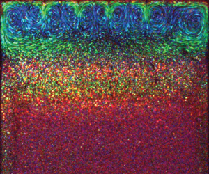
The mechanism forming LRSs in SHC can be investigated via an analogue system, the so-called Rayleigh–Bénard–Poiseuille (RBP) convection. The RBP convection is a Poiseuille flow subjected to an unstable vertical temperature gradient environment that potentially drives Rayleigh–Bénard convection. The similarity between RBP convection and SHC is illustrated in figures 12(a) and 12(b). The RBP convection has been studied especially for characterising heat transfer processes of air ducts, and an early comprehensive review for this problem is found in Nicolas (Reference Nicolas2002). A mean flow with a parabolic (Poiseuille) velocity profile is subjected to a destabilising vertical temperature difference  $\Delta T$ across the full height $H_{v}$. Accordingly, the RBP convection can be characterised by the vertical Rayleigh number, $Ra_{v} = g\alpha \Delta T H_{v}^3/(\kappa \nu )$. Note that the mean flow itself does not contribute to the development of LRSs. However, the LRS formation happens when the system is closed in the spanwise direction. The presence of the lateral walls supports the corner roll formation due to the pressure gradient at the corner, and this corner roll triggers the generation of LRSs towards the interior. As a result, LRSs are aligned in the spanwise direction (Akiyama, Hwang & Cheng Reference Akiyama, Hwang and Cheng1971; Pabiou, Mergui & Benard Reference Pabiou, Mergui and Benard2005; Mergui, Nicolas & Hirata Reference Mergui, Nicolas and Hirata2011; Taher & Abid Reference Taher and Abid2018; Taher et al. Reference Taher, Ahmed, Haddad and Abid2021). Since $Ra$ does not change along the streamwise direction, the characteristics of LRSs do not change in space under fixed environments. By contrast, in the case of SHC, the shallow streaming region of the main circulation plays a similar role to that of the main flow of RBP convection. In addition, the overturning circulation transports heat from the highest temperature surface ( $0\leq x \lesssim W_2$). This horizontal heat transport spontaneously creates an unstable temperature gradient in the downstream uppermost region, as the surface temperature is lower than that upstream. For the onset of Rayleigh–Bénard-like convection, we can define a local Rayleigh number considering the unstable layer thickness as $Ra_{t} = g\alpha \Delta T_{t} \delta _{t}^3/(\kappa \nu )$, where $\Delta T_{t}$ is the temperature difference imposed over $\delta _{t}$. As shown in figure 11, $\delta _{t}$ and $\Delta T_{t}$ change along the streamwise direction, and these changes eventually result in an increase or decrease of $Ra_{t}$. Once $Ra_{t}$ exceeds the critical value, the confining effect will support the formation of a secondary flow at the top-lateral corners following the same scenario as that in RBP convection. This corner roll formation will occur irrespective of the onset of Rayleigh–Bénard-like convection, as shown in figure 4(a), i.e. weak rolls are formed even in a Q2-D state. The characteristic length of this initial secondary circulation depends on $\delta _{s}$, the thickness of the downstream flow and the apparent Rayleigh number of the LRSs is $Ra_{s} = g\alpha \Delta T_{s} \delta _{s}^3/(\kappa \nu )$, where $\Delta T_{s}$ is the temperature difference imposed over $\delta _{s}$. This roll formation progresses towards the interior and the downstream directions. Unlike the RBP convection, the secondary flow on the lateral walls is always downward because of the surface and the spanwise confinement. This regulates the spinning direction (or the sign of vorticity) of the LRSs formed upstream (see figure 5). Such LRSs are stable over time. A significant difference between RBP convection and SHC is their lower boundary. In the latter case, the bottom boundary is open, leading to spatial changes in the characteristics of LRSs. In figure 12(c), particle pathline images at two different $x$ positions for the case of the 3-D state ( $Pe = 5.5\times 10^4$ and $Ri=0.027$) are shown. Since the images are compiled using the colour images of the TLC particles, the colour qualitatively indicates the temperature fields, where blue is hot and red is cold. In the left panel, there are corner rolls at the top boundaries and the rest is stably stratified. In the right panel, reddish or greenish cold fluids are transported from the top and the LRSs occupy the whole spanwise domain, while the rest maintains stratification. The downstream region has thicker LRSs than the upstream region, as explained above.
Schematic illustrations of LRS formation mechanism in (a) RBP convection and (b) SHC, and (c) colour particle pathline images of the TLC particles showing the LRS formations at different  $x$ positions ( $Pe = 5.5\times 10^4$ and $Ri=0.027$). The colour in (c) qualitatively indicates the temperature distribution, and the flow directions are indicated by the arrows.

Inspired by the RBP convection system described above, we examine a set of streamwise flow parameters to characterise the properties of the overturning circulation. Figure 13 displays  $\delta _{s}/H$ and $\delta _{t}/H$, $\Delta T_{s}/\Delta \theta$ and $\Delta T_{t}/\Delta \theta$, $Ra_{s}$ and $Ra_{t}$ and the number of rolls $N_{roll}$ along the streamwise direction, $x/W$, for three Péclet numbers. Panels (a,d,g,j) show a Q2-D state with $Pe = 7.2\times 10^3$ and $Ri=80$. In contrast, panels (b,e,h,k) and (c, f,i,l) illustrate 3-D state cases with $Pe = 3.7\times 10^4$ and $Ri=0.293$, and $Pe = 5.5\times 10^4$ and $Ri=0.027$, respectively. Figure 13(a–c) shows $\delta _{s}/H$ and $\delta _{t}/H$; the results show that both $\delta _{s}$ and $\delta _{t}$ thicken downstream, almost monotonically, for the higher $Pe$ cases.
Streamwise-dependent features of RBP convection for different  $Pe$ conditions: (a,d,g,j) $Pe = 7.2\times 10^3$, (b,e,h,k) $Pe = 3.7\times 10^4$ and (c, f,i,l) $Pe = 5.5\times 10^4$. Thicknesses of the downstream region $\delta _{s}$ and the unstable layer $\delta _{t}$, local vertical temperature difference $\Delta T_{s}$ and $\Delta T_{t}$, local Rayleigh number $Ra_{s}$ and $Ra_{t}$ and the number of LRSs $N_{roll}$ are shown respectively from top to bottom. Grey regions, $x/W < 0.25$, correspond to the heated regions with a surface temperature of $T_2$. Dashed-dotted lines and dotted lines correspond to critical Rayleigh numbers for no-slip $Ra_{cn}$ and free-slip conditions $Ra_{cf}$, respectively. The values of $N_{roll}$ are not available for (a,d,g,j) because of the absence of LRSs.

Figure 13(d–f) shows the vertical temperature differences  $\Delta T_{s}/\Delta \theta$ and $\Delta T_{t}/\Delta \theta$. For the Q2-D state shown in figure 13(a,d,g,j), $\Delta T_{t}$ becomes positive in a highly limited region immediately after $x=W_2$, and $\Delta T_{s}$ is always negative. The latter implies that the system is mostly stably stratified over $\delta _{s}$. On the other hand, $\Delta T_{t}$ and $\Delta _{s}$ become positive at $x > W_2$ for the 3-D state cases shown in figures 13(b,e,h,k) and (c, f,i,l). Such unstable temperature distributions decay gradually downstream.
We compute and plot the local Rayleigh numbers,  $Ra_{s}$ and $Ra_{t}$, as a function of $x/W$ in figure 13(g–i). For reference, the critical Rayleigh numbers for the case of no-slip boundaries, $Ra_{cn}=1708$, and free-slip boundaries, $Ra_{cf} = 657.5$ (Chandrasekhar Reference Chandrasekhar1961; Cross & Hohenberg Reference Cross and Hohenberg1993), are denoted by the dashed-dotted and dotted lines, respectively. For the 2-D case, $Ra_{t}$ does not exceed the critical values. By contrast, for the 3-D state cases, $Ra_{t}$ typically starts around $10^3$ at $x\sim W_2$ which is quite close to the critical values. This result indicates that the formation of the LRSs is associated with the critical Rayleigh numbers. The critical Rayleigh number $Ra_{c}$ is expressed as
 \begin{equation} Ra_{c} = \frac{g\alpha\Delta\theta\delta_{c}^3}{\nu\kappa} = \frac{Pe_{c}^2}{Pr}\frac{\delta_{c}^3}{hW^2}, \end{equation}
where  $\delta _{c}$ is the minimum thickness corresponding to the potential maximum vertical temperature difference $\Delta \theta$. Here, $Pe_{c}$ is the critical Péclet number for the onset of Rayleigh–Bénard-like convection. Accordingly, $Pe_{c}$ can be expressed as
 \begin{equation} Pe_{c} = \left(Pr\,Ra_{c}\frac{h\,W^2}{\delta_{c}^3}\right)^{1/2}. \end{equation}
Assuming that  $Ra_{c} \sim 10^3$ and $\delta _{c} \approx \delta _{t}$, $Pe_{c}$ can be estimated from the experimental results. Even though $\delta _{t}$ changes with $x$, it varies approximately in the range $1$–
$1$– $5~{\rm mm}$. Using these values, $Pe_{c}$ is estimated as $Pe_{c} \gtrsim 10^4$, which is consistent with the empirical critical values $Pe_{c}\approx 3.3\times 10^4$ shown in figure 7. This consistency supports the above explanation that LRSs originated from Rayleigh–Bénard convection. The apparent Rayleigh number $Ra_{s}$ of the LRSs ranges in $O(10^3$– $10^4)$, meaning that the downstream region maintains the supercriticality. For the case shown in figure 13(b,e,h,k), the Péclet number is marginally bigger than its critical empirical value for which SHC transitions from a Q2-D flow to a 3-D flow. In this case, $Ra_{s}$ remains supercritical and almost uniform along $x$. However, for the case with the greatest $Pe$, shown in figure 13(c, f,i,l), $Ra_\delta$ has a quasi-linear increase.
Figure 13(j–l) shows the number of LRSs  $N_{roll}$ in the $y$–
$y$– $z$ planes. the value of $N_{roll}$ is zero in the region $0\leq x/W \leq 0.25$, and the first pair of LRSs emerges from the lateral boundaries downstream $x>W_2$. The LRS formation propagates towards the interior, making $N_{roll}$ increase until the spanwise domain is fully occupied by LRSs. The full development of LRSs is achieved at $x/W \sim 0.5$. After the full development, the LRSs start to merge with each other and this trend appears as the decrease of $N_{roll}$. The coalescence keeps the aspect ratio of the LRSs almost constant, not far from unity, over the whole downstream region, as the roll regions are thickening downstream.
Summing up, the streamwise dependent features shown in figure 13 provide robust evidence that LRSs developed in SHC obey analogue physical processes to those controlling the transition to 3-D flow in RBP convection: it is a localised phenomenon that spontaneously happens at high- $Pe$ conditions ( $Pe \gtrsim 3.3\times 10^{4}$), leading to supercritical $Ra_{t}$, that support (i) local heat transport via Rayleigh–Bénard-like convection, (ii) the vertical expansion of the overturning circulation and (iii) ultimately the enhancement of the horizontal transport.
5.2. Mechanical energy conversion
As shown in figure 9, only a small portion of the APE is converted into KE in SHC. The latter implies that SHC is a system in which most of the available energy is utilised in sustaining the stratification and mixing of the overturning region. To quantify the mechanical energy conversion, we diagnose the mixing efficiency  $\eta$ defined as $\eta = (\varPhi _{d} - \varPhi _{i}) / (\varPhi _{d} - \varPhi _{i} + \epsilon )$ (Peltier & Caulfield Reference Peltier and Caulfield2003). Here, $\varPhi _{d} = -\kappa g\int _V ({\rm d}z_{\star }/{\rm d}\rho )\,|\boldsymbol {\nabla } \rho |^2\,{\rm d}V$ is the rate at which $E_{ap}$ depletes due to the irreversible scalar mixing controlling $\rho$ and $\varPhi _{i} = -\kappa g WL (\rho _{top} - \rho _{bottom})$ is the conversion rate from internal energy to PE, where $\rho _{top}$ and $\rho _{bottom}$ are the laterally averaged densities at the top and the bottom boundaries, respectively (Winters et al. Reference Winters, Lombard, Riley and D'Asaro1995). Also, $\epsilon = \rho _0\nu \int _V (|\boldsymbol {\nabla } u|^2 + |\boldsymbol {\nabla } v|^2 + |\boldsymbol {\nabla } w|^2)\,{\rm d}V$ is the KE dissipation rate. Irrespective of the conditions, we obtained $\eta \approx 0.99$, close to unity. Please note that the density (temperature) fields are reconstructed under 2-D assumption (4.6), and the energy budget of the system is not fully closed. Hence, one can expect that our estimation of $\eta$ may differ from systems that fully close the energy budget. In HC systems, $\eta \rightarrow 1$ is predicted theoretically as an upper bound for the inviscid regime with very large $Ra$ (Scotti & White Reference Scotti and White2011), whereas numerical simulation shows a slightly smaller value, $\eta = 0.923$ (Gayen et al. Reference Gayen, Griffiths, Hughes and Saenz2013).
Considering the difference in the effective lower boundary of the overturning circulation in SHC (stably stratified layer) and HC (no-slip wall boundary), one would expect SHC to develop less viscous dissipation than HC. In SHC, the lower stably stratified layer acts as an adjustable ‘soft no-slip’ boundary, unlike the rigid no-slip bottom set in HS, in which a vigorous flow has no other option than to intensify its shear rate rather than mix and expand as in the case of SHC. Despite this fundamental difference, the estimated mixing efficiency for SHC remains in close agreement with values obtained through numerical simulations and upper bound scalings for HC.
6. Concluding remarks
This paper investigated experimentally the fluid dynamics of SHC, the overturning circulations driven by surface differential heating in stably stratified fluid bodies. The designed experimental framework allowed us to measure the quasi-instantaneous 3-D velocity field by utilising multiple cameras and scanning light blade systems. Moreover, from the measured velocity field and prescribed boundary conditions, we reconstructed the Q2-D temperature field that fulfils the steady state momentum balance achieved in the experiments.
SHC can be described by the Rayleigh number  $Ra$, representing the destabilising effect of buoyancy, and the bulk Richardson number $Ri$, representing the stabilising effect of background stratification. We derived a characteristic length scale from the system's parameters which predicts the overturning circulation thickness and its characteristic velocity $U_{adv}$ by accounting for the hypothetical equilibrium height of fluid parcels. From these scales, we define the Péclet number, $Pe = U_{adv}W/\kappa = [(Pr\,Ra)/(\mathcal {A}\,Ri\,\varTheta )]^{1/2}$, which consolidates all the dimensionless parameters involved in SHC, including the vertical and horizontal temperature difference ratio $\varTheta$, the basin aspect ratio $\mathcal {A}$ and the Prandtl number $Pr$ in addition to $Ra$ and $Ri$.
$Ri$.
We observed experimentally the fluid dynamics of SHC, the formation of a Q2-D overturning circulation confined at the upper region above the stably stratified layer and its transition towards 3-D LRSs. Here, we show theoretically and experimentally that  $Pe$ governs the global properties, such as the maximum streamfunction $\psi _{max} \propto Pe$ and the available mechanical energy of the system. Furthermore, we showed that local properties, such as the flow dimensionality, are ruled by $Pe$. We also discussed mechanical energy conversion, finding that the irreversible mixing of SHC is extremely high, in agreement with the theoretical and numerical results of HC.
In conclusion, our study provides insights into stratified fluid environments that experience horizontal density gradients, such as lakes, oceans and atmospheres. There is a wide range of aspects that future research could explore via theoretical studies, laboratory experiments and numerical simulations, for instance: (i) the conditions for developing secondary LRS; (ii) the transition towards turbulence, potentially at higher  $Pe$; (iii) the system response to different $Pr$ and $\mathcal {A}$; (iv) the effects of lateral confinements; and (v) the impact of rotation.
Acknowledgements
The authors are grateful for the helpful discussions with Dr T. Miyagoshi (Japan Agency for Marine-Earth Science and Technology, JAMSTEC). The authors also thank the anonymous reviewers for encouraging and constructive comments. D.N. and H.N.U. acknowledge the support of the Start-up fund at the Department of Earth and Environmental Science, University of Pennsylvania.
Fundings
This work was partially supported by the Grant-in-Aid for the Japan Society for the Promotion of Science (JSPS) Fellows (grant no. 19JP19006).
Declaration of interests
The authors report no conflict of interest.


 Open access

