





Foreword
In the spirit of this special issue, we would like to say a few words about Professor Andrew Bassom, written by co-author Neville Fowkes.
Andrew’s contributions to applied maths are major with approximately 200 career research articles. One of Andrew’s special skills is his ability to write mathematics beautifully, as is testified by the authors of this article. His writing is concise, with everything in but no excess, but importantly the results “tell the historic story”.
Here is a brief history on boundary tracing and dip-coating, and Andrew’s involvement.
In 1998, I was visiting The Mathematical Institute at Oxford and DuPont de Nemours challenged the research group to solve the capacitor dipping problem, referred to as “the mooning problem”. Determining the capillary height rise in a wedge is fundamentally a Laplace–Young problem, with “weird results”; the height rise can be finite or infinite, or with or without a discontinuity at the corner; the mooning problem was “hard”. Anyhow, we (John and Hilary Ockendon, John King, Malcolm Hood, John Norbury, Graeme Sander and myself) produced interesting research results, but couldn’t solve the mooning problem. My thought was that rounding the corner was the way to go. I brought the problem back to the University of Western Australia and gave the challenge to Michael Anderson, an exceptional PhD student of mine. I asked him to first look at a simpler but related Helmholtz equation problem which admits an exact solution in a right-angled corner domain; it should have been easy “to round the corner” using a perturbation approach, but he failed to produce results for really surprising reasons. It turns out that the known exact solution in the right-angled wedge was also the exact solution in regions with a rounded corner boundary that could be simply constructed using “boundary tracing” as described in the main text. Furthermore, there were an infinite number of boundaries with the same exact solution that could be constructed using tracing [Reference Anderson, Bassom and Fowkes4]. Following on from this, Michael produced an even more remarkable result for the Laplace–Young equation with contact condition. The only known exact solution was the one-dimensional solution corresponding to the height rise of liquid against a flat wall. Michael found that he could use tracing to determine a “multiply-infinite” number of domains corresponding to the same solution and satisfying the contact condition; these domains corresponded to a roughening of the plane wall [Reference Anderson, Bassom and Fowkes2]. This was a seemingly ridiculous result; it took us ages to convince ourselves that there wasn’t a simple error! Of course, all high school science students know how careful one has to be to clean the surfaces in capillary experiments; this was a really important result! Michael then went on to obtain exact results (new boundaries) for “all” the classical two-dimensional partial differential equations, and he developed “the theory”; really pretty work. He finished his thesis and went off leaving a large volume of really important results and ideas “not yet published” in external journals.
Sometime later, I put together the crude first drafts of Michael’s work and kindly Andrew offered to assist with the write up. Given the controversial and unexpected nature of the tracing technique results, this was a daunting task. Anyhow, Andrew greatly improved my drafts and the major results were published in three Proceedings articles; the articles were accepted immediately and published in 2006/2007 and are a real pleasure to read. In fact, later, we were congratulated as being the most successful Proceedings of the Royal Society A contributors in that year.
Thank you Andrew!
Well, the mooning problem fell by the wayside while all the above was happening. It was up to another exceptional student (Conway Li) to use tracing to complete the mooning problem, address the Laplace–Young wedge problems, and obtain other important radiation and conformal mapping results using tracing. Miccal Matthews, Brendan Florio and myself were Conway’s supervisors. The mooning problem (presented here) filled one of the last chapters of his thesis; the important wedge problem results are yet to be published.
Nev, Miccal, Brendan, Conway.
1 Introduction
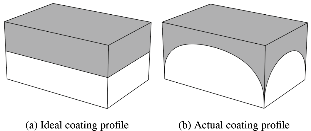
In the industrial process of capacitor production, (1 mm by 0.5 mm) rectangular “slabs” of silicon are partially dip-coated in molten metal baths and removed, see Figure 1. During this process, the molten metal rises up the slab faces and dips near the corners due to the effects of surface tension. After removal from the bath, the metal on the slab solidifies, retaining the undesirable “mooning shape”; with such a shape, the metal caps of the capacitor are likely to split off. Ideally, in this context, the contact line should be horizontal, and the suggestion is that this may be achieved by either rounding the corners or roughening the surfaces of the slab, or both. The modifications should be minor so that the slab remains essentially rectangular. A suitably modified mechanical tumbler may achieve such a result. It should be noted that the problem of reducing surface tension effects near corners or edges is of major interest in many industrial dip-coating and spray-painting processes.
Dip-coating a rectangular object (grey) in a liquid (white). The aim is to produce the ideal coating profile by rounding the corner and roughening the surface.

The height rise $\eta (x,y, \gamma )$
of the free surface of a liquid due to the presence of a partially submerged object with vertical sides is determined by the (dimensionless) Laplace–Young equation
$\eta (x,y, \gamma )$
of the free surface of a liquid due to the presence of a partially submerged object with vertical sides is determined by the (dimensionless) Laplace–Young equation
 $$ \begin{align} {\boldsymbol \nabla} \cdot \left(\frac{{\boldsymbol \nabla}\eta}{\sqrt{1+({\boldsymbol \nabla}\eta)^2}}\right)= \eta \quad \mathrm{in} \ \varOmega, \end{align} $$
with the boundary/contact condition
 $$ \begin{align} \left(\frac{{\boldsymbol \nabla}\eta}{\sqrt{1+({\boldsymbol \nabla}\eta)^2}}\right) \cdot \textbf{n}=\cos \gamma \quad \mathrm{around} \ \partial\varOmega. \end{align} $$
Here, $\varOmega $
is the (infinite) domain occupied by the liquid surrounding the solid object with boundary
$\varOmega $
is the (infinite) domain occupied by the liquid surrounding the solid object with boundary $\partial \varOmega $
. The height rise,
$\partial \varOmega $
. The height rise, $\eta $
, and the spatial variables x and y have been nondimensionalized using the capillary length to scale. The capillary length is given by
$\eta $
, and the spatial variables x and y have been nondimensionalized using the capillary length to scale. The capillary length is given by $\sqrt {\sigma /\rho g}$
, where
$\sqrt {\sigma /\rho g}$
, where $\sigma $
is the surface tension,
$\sigma $
is the surface tension, $\rho $
the density difference and g the gravitational constant. The contact angle is
$\rho $
the density difference and g the gravitational constant. The contact angle is $\gamma $
and the liquid is assumed to wet the solid so that
$\gamma $
and the liquid is assumed to wet the solid so that $0<\gamma \le \pi /2$
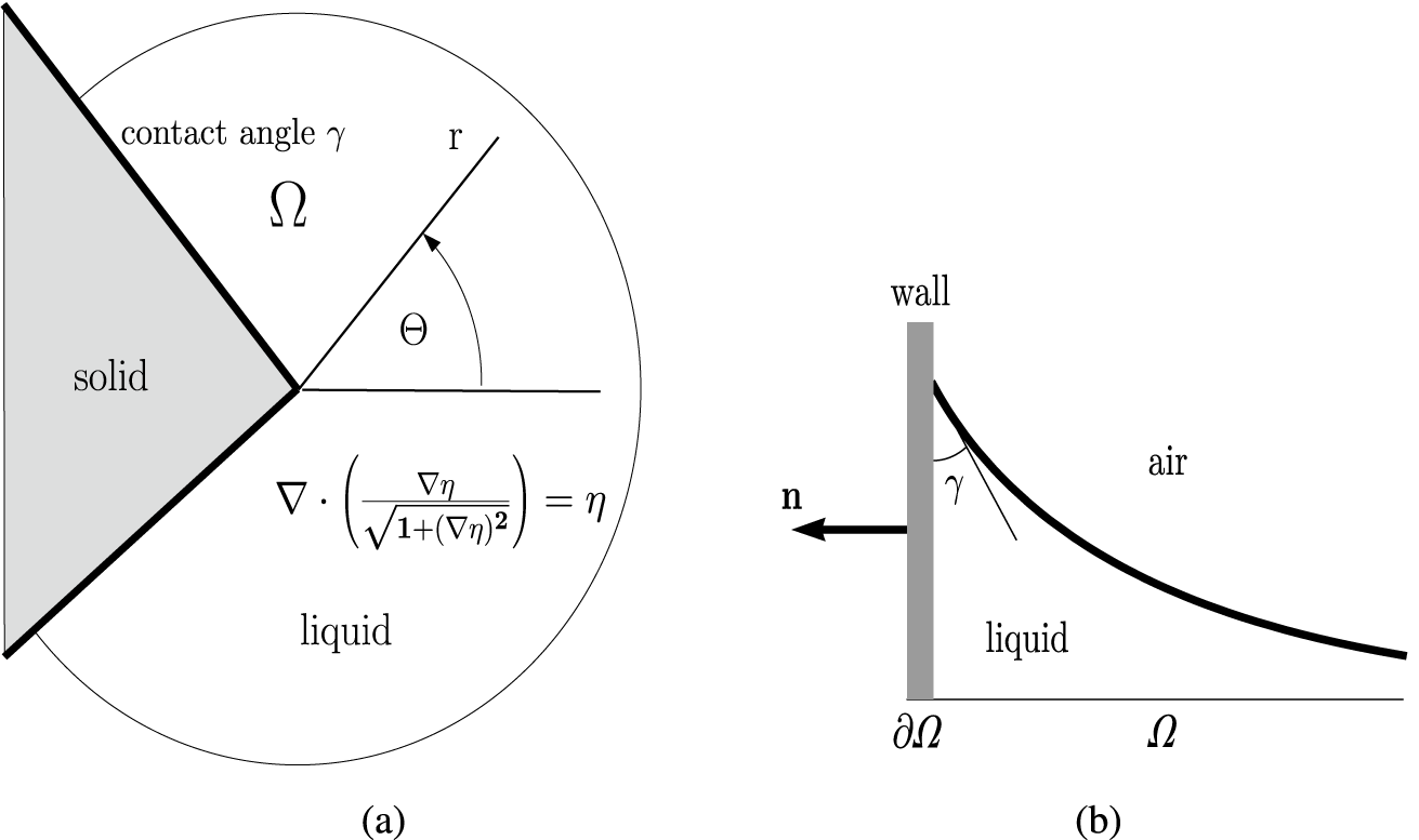
, see Figure 2.
$0<\gamma \le \pi /2$
, see Figure 2.
(a) The unmodified wedge solution domain $\varOmega $
(
$\varOmega $
( $- 3 \pi /4<\varTheta <3 \pi /4$
). The corner of the wedge is to be modified by rounding the rectangular corner of the solid and roughening its surface. (b) The liquid/solid contact angle.
$- 3 \pi /4<\varTheta <3 \pi /4$
). The corner of the wedge is to be modified by rounding the rectangular corner of the solid and roughening its surface. (b) The liquid/solid contact angle.

In our case, the object (before surface modification) is rectangular and, if we assume its length scale is much greater than the capillary length, then we can equivalently look at the infinite wedge problemFootnote 1, see Figure 2. With this geometry, it is convenient to introduce polar coordinates $(r, \varTheta )$
to specify the solution domain
$(r, \varTheta )$
to specify the solution domain $\varOmega $
, where
$\varOmega $
, where $0<r<\infty $
, and
$0<r<\infty $
, and $-\alpha \le \varTheta \le \alpha $
measures the angular displacement away from the line of symmetry and
$-\alpha \le \varTheta \le \alpha $
measures the angular displacement away from the line of symmetry and $2 \alpha $
is the wedge angle of the domain. In the case of particular interest here, the wedge angle is
$2 \alpha $
is the wedge angle of the domain. In the case of particular interest here, the wedge angle is $2\alpha = {3 \pi }/{2}$
. In the absence of boundary modification, the contact line dips abruptly near the corner over a length scale of order unity, with the height rise
$2\alpha = {3 \pi }/{2}$
. In the absence of boundary modification, the contact line dips abruptly near the corner over a length scale of order unity, with the height rise $\eta (0, \varTheta , \gamma )$
finite. Ideally, this contact line would be horizontal and we seek to (slightly) modify the corner boundary shape to achieve this.
$\eta (0, \varTheta , \gamma )$
finite. Ideally, this contact line would be horizontal and we seek to (slightly) modify the corner boundary shape to achieve this.
The only known exact (but implicit) solutions for the Laplace–Young equation are the one-dimensional plane wall solution (corresponding to a wedge angle $2 \alpha =\pi $
) and the (related) channel solution, and were obtained by Young in 1804. The plane wall solution
$2 \alpha =\pi $
) and the (related) channel solution, and were obtained by Young in 1804. The plane wall solution $\eta (y,\gamma )$
corresponding to contact angle
$\eta (y,\gamma )$
corresponding to contact angle $\gamma $
is given by
$\gamma $
is given by
 $$ \begin{align} y=\mathrm{arccosh}(2/\eta)-\mathrm{arccosh}(2/h_{\gamma})+\Big[\!\sqrt{4-h_{\gamma}^2}-\sqrt{4-\eta^2}\Big], \end{align} $$
where
 $$ \begin{align} h_{\gamma}=\sqrt{2(1-\sin \gamma)}; \end{align} $$
here, y measures distance away from the wall and $h_{\gamma }$
is the height rise up the wall.
$h_{\gamma }$
is the height rise up the wall.
Aside: Note that there are dramatic changes in the solution behaviour as the wedge angle changes and asymptotic results have been obtained [Reference Concus and Finn6, Reference Concus and Finn7, Reference Miersemann13–Reference Norbury, Sander and Scott15]. The height rise is infinite in the corner in the small wedge angle range $\alpha <\alpha ^{c1}$
with
$\alpha <\alpha ^{c1}$
with $\alpha ^{c1}={\pi }/{2} -\gamma $
. In the medium range
$\alpha ^{c1}={\pi }/{2} -\gamma $
. In the medium range $\alpha ^{c1}< \alpha < \alpha ^{c2}$
with
$\alpha ^{c1}< \alpha < \alpha ^{c2}$
with $\alpha ^{c2}= {\pi }/{2} +\gamma $
, the solution is finite and locally planar, whereas in the large wedge angle (re-entrant corner) case
$\alpha ^{c2}= {\pi }/{2} +\gamma $
, the solution is finite and locally planar, whereas in the large wedge angle (re-entrant corner) case $\alpha> \alpha ^{c2}$
, the height rise is finite but the contact line slope is infinite in the corner. In our case, we have
$\alpha> \alpha ^{c2}$
, the height rise is finite but the contact line slope is infinite in the corner. In our case, we have $\alpha = {3 \pi }/{4 }$
so we are in the re-entrant wedge angle range for surface wetting liquids. The re-entrant corner case is not without controversy. In the general case, the height rise can be discontinuous across the edge, as observed by Korevaar [Reference Korevaar9] and King et al. [Reference King, Ockendon and Ockendon8]; however, this situation can only occur in asymmetric domain cases.
$\alpha = {3 \pi }/{4 }$
so we are in the re-entrant wedge angle range for surface wetting liquids. The re-entrant corner case is not without controversy. In the general case, the height rise can be discontinuous across the edge, as observed by Korevaar [Reference Korevaar9] and King et al. [Reference King, Ockendon and Ockendon8]; however, this situation can only occur in asymmetric domain cases.
Returning to the corner modification problem, it is of course impossible to produce results for all possible corner roundings; we need a representative sample. Boundary tracing is a procedure that is ideally suited to explore the effect of various boundary changes on the solution behaviour. This procedure is somewhat novel, but has been successfully employed to obtain exact results for the solution of two-dimensional (2D) boundary value problems (BVPs) in various applications with nonstandard domains, including problems in radiation and root growth, amongst others [Reference Anderson, Bassom and Fowkes4, Reference Anderssen, Hale and Radok5, Reference Li, Florio, Fowkes and Matthews10–Reference McNabb, Wake, Lambourne and Anderssen12]. The procedure is elementary and can be applied in our case without a detailed reading of the underlying theory described in [Reference Anderson, Bassom and Fowkes3]. One simply takes a known solution of the field equation and determines new boundaries along which the prescribed boundary condition is satisfied. Consider a trivial example where the field equation has the solution $g(x,y) = x^2 + y^2$
. Using this solution, we could define a boundary
$g(x,y) = x^2 + y^2$
. Using this solution, we could define a boundary $\partial \varOmega $
such that the boundary condition
$\partial \varOmega $
such that the boundary condition $g(x,y) = 1$
is satisfied on
$g(x,y) = 1$
is satisfied on $\partial \varOmega $
: this would be the circle of radius
$\partial \varOmega $
: this would be the circle of radius $1$
. The boundary tracing method is a generalized procedure that can be used to inscribe boundaries for any flux-type boundary condition. For an example in the surface tension context, the known plane wall Laplace–Young solution (1.3) was used to obtain exact results for rough walls [Reference Anderson, Bassom and Fowkes2]. The field solution used for constructing new boundaries may be an exact analytic solution as in the plane wall Laplace–Young situation, but a numerical solution can also be used and is needed here.
$1$
. The boundary tracing method is a generalized procedure that can be used to inscribe boundaries for any flux-type boundary condition. For an example in the surface tension context, the known plane wall Laplace–Young solution (1.3) was used to obtain exact results for rough walls [Reference Anderson, Bassom and Fowkes2]. The field solution used for constructing new boundaries may be an exact analytic solution as in the plane wall Laplace–Young situation, but a numerical solution can also be used and is needed here.
1.1 Boundary tracing
The boundary tracing technique takes a known solution $\eta (x,y)$
of a 2D field equation and considers general flux type boundary conditions of the form
$\eta (x,y)$
of a 2D field equation and considers general flux type boundary conditions of the form
 $$ \begin{align} \boldsymbol{{\nabla}} \eta(x,y) \cdot \textbf{n} =F(\eta, |\boldsymbol{\nabla} \eta |, x,y), \end{align} $$
where $\textbf {n}$
is the normal to the boundary and the flux function F is an arbitrary function of its arguments. This boundary condition can be thought of as a geometric constraint on the orientation of possible boundaries defined by
$\textbf {n}$
is the normal to the boundary and the flux function F is an arbitrary function of its arguments. This boundary condition can be thought of as a geometric constraint on the orientation of possible boundaries defined by $\textbf {n}$
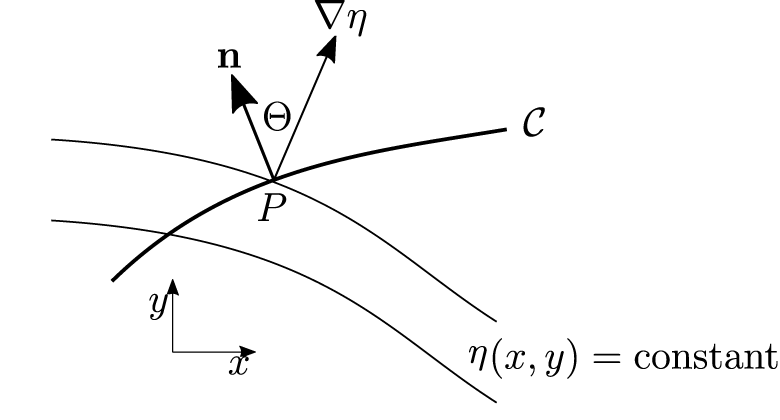
, see Figure 4. Evidently, see (1.5), if
$\textbf {n}$
, see Figure 4. Evidently, see (1.5), if $P(x,y)$
is a point in the solution domain, then no such orientation is possible unless
$P(x,y)$
is a point in the solution domain, then no such orientation is possible unless
 $$ \begin{align*} | \boldsymbol{\nabla} \eta(x,y)| \ge |F|, \end{align*} $$
or, equivalently,
 $$ \begin{align*} \varPhi \ge 0, \quad \mathrm{where}\ \varPhi= (\boldsymbol{\nabla} \eta)^2-F^2 \end{align*} $$
is referred to as the viability function. This function defines the viable domain for tracing with the critical or terminal curve given by $\varPhi =0$
separating it from the nonviable domain. Within this viable domain, there will be two orientations for a possible boundary symmetrically disposed about the normal
$\varPhi =0$
separating it from the nonviable domain. Within this viable domain, there will be two orientations for a possible boundary symmetrically disposed about the normal $\textbf {n}$
. If
$\textbf {n}$
. If $(x(s), y(s))$
defines such a boundary curve as a function of arc length s, then a direct application of (1.5) gives
$(x(s), y(s))$
defines such a boundary curve as a function of arc length s, then a direct application of (1.5) gives
 $$ \begin{align*} (\eta_x, \eta_y) \cdot(y_s,-x_s)=F,\end{align*} $$
which, together with the arc length requirement
 $$ \begin{align*} {x_s}^2 + {y_s}^2=1, \end{align*} $$
gives (solving for $(x_s, y_s)$
)
$(x_s, y_s)$
)
 $$ \begin{align} \frac{dx}{ds} &= \frac{-\eta_y F \pm \eta_x \sqrt{\varPhi}}{(\boldsymbol{\nabla} \eta)^2}, \end{align} $$
 $$ \begin{align} \frac{dy}{ds} &= \frac{+\eta_x F \pm \eta_y \sqrt{\varPhi}}{(\boldsymbol{\nabla} \eta)^2}. \end{align} $$
Note that the two solution branches correspond to the $\pm $
sign in front of the square root and that the argument of the square root is real if
$\pm $
sign in front of the square root and that the argument of the square root is real if $\varPhi \ge 0$
, that is, if
$\varPhi \ge 0$
, that is, if $(x,y)$
is within the viable domain. Recall that
$(x,y)$
is within the viable domain. Recall that $\eta (x,y)$
is a prescribed exact solution of the defining field equation (and
$\eta (x,y)$
is a prescribed exact solution of the defining field equation (and $\varPhi , F$
are known functions of
$\varPhi , F$
are known functions of $(\eta (x,y), x,y)$
), so these equations are simply ordinary differential equations for determining possible boundary “traces”
$(\eta (x,y), x,y)$
), so these equations are simply ordinary differential equations for determining possible boundary “traces” $(x(s),y(s))$
coming away from any arbitrary point
$(x(s),y(s))$
coming away from any arbitrary point $(x(0),y(0))$
in the viable domain. These traces can be patched together in almost any way to produce an infinite number of new boundaries. In the wedge problem of interest here, boundaries that round the corner are thus constructed.
$(x(0),y(0))$
in the viable domain. These traces can be patched together in almost any way to produce an infinite number of new boundaries. In the wedge problem of interest here, boundaries that round the corner are thus constructed.
In Section 2, we obtain contact line solutions corresponding to rounded corners using boundary tracing. We show that such corner modifications do not significantly flatten the contact line. Then, in Section 3, we consider the effect of surface roughening, again using boundaries generated using boundary tracing. The results show that the correct combination of corner rounding with surface roughening results in a horizontal contact line. Conclusions are drawn in Section 4.
2 Corner rounding
To apply boundary tracing in our case, it is necessary to work with a prescribed solution $\eta (r, \varTheta , \gamma )\equiv \eta (x,y, \gamma )$
of the Laplace–Young equation (1.1) in the
$\eta (r, \varTheta , \gamma )\equiv \eta (x,y, \gamma )$
of the Laplace–Young equation (1.1) in the $\alpha = 3\pi /4$
wedge. Since no such exact solution is known in our wedge region, we need to use numerically generated results. An adapted finite-element Mathematica program was used as described in Appendix A. A typical solution corresponding to a specific contact angle (
$\alpha = 3\pi /4$
wedge. Since no such exact solution is known in our wedge region, we need to use numerically generated results. An adapted finite-element Mathematica program was used as described in Appendix A. A typical solution corresponding to a specific contact angle ( $\gamma = {60}^{\circ }$
) is displayed in Figure 3.
$\gamma = {60}^{\circ }$
) is displayed in Figure 3.


Boundary tracing geometry. The orientation $\textbf {n}$
of a potential boundary trace
$\textbf {n}$
of a potential boundary trace $\cal {C}$
at a point P relative to the level curve passing through P has to be such that
$\cal {C}$
at a point P relative to the level curve passing through P has to be such that $ \cos \varTheta =|F|/ |\nabla \eta |$
.
$ \cos \varTheta =|F|/ |\nabla \eta |$
.

We now proceed with boundary tracing. The contact condition in flux form is given by
 $$ \begin{align} \nabla \eta \cdot \textbf{n}= F=\cos\gamma \sqrt{1 + (\boldsymbol{\nabla} \eta)^2}, \end{align} $$
with the viability function given by
 $$ \begin{align} \varPhi &= (\boldsymbol{\nabla} \eta)^2 - F^2 \nonumber\\ &= \sin^2\gamma \, [(\boldsymbol{\nabla} \eta)^2 - \cot^2\gamma]. \end{align} $$
Recall that tracing is only possible at points $(x,y)$
in the solution domain where
$(x,y)$
in the solution domain where $\varPhi \ge 0$
; in our case, this gives
$\varPhi \ge 0$
; in our case, this gives
 $$ \begin{align*} |\boldsymbol{\nabla} \eta | \ge \cot\gamma. \end{align*} $$
In geometric terms, the $\eta (x,y, \gamma )$
surface steepness must be greater than, or equal to, that defined by the contact angle
$\eta (x,y, \gamma )$
surface steepness must be greater than, or equal to, that defined by the contact angle $\gamma $
.
$\gamma $
.
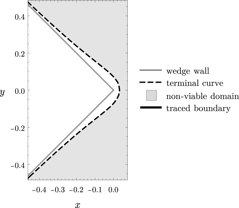
The viable region for tracing lies between the terminal curve $\boldsymbol {\nabla } \eta = \cot \gamma $
, which is determined using the computed solution
$\boldsymbol {\nabla } \eta = \cot \gamma $
, which is determined using the computed solution $\eta (x, y, \gamma )$
and the wedge walls. The results for the contact angle
$\eta (x, y, \gamma )$
and the wedge walls. The results for the contact angle $\gamma = 60^{\circ }$
case are shown in Figure 5. The terminal curve rounds the corner and asymptotes to the wedge walls far from the corner.
$\gamma = 60^{\circ }$
case are shown in Figure 5. The terminal curve rounds the corner and asymptotes to the wedge walls far from the corner.
The nonviable domain $\varPhi < 0$
for
$\varPhi < 0$
for $\gamma = {60}^{\circ }$
is shaded. Tracing is possible in the viable region between this domain and the wedge walls.
$\gamma = {60}^{\circ }$
is shaded. Tracing is possible in the viable region between this domain and the wedge walls.

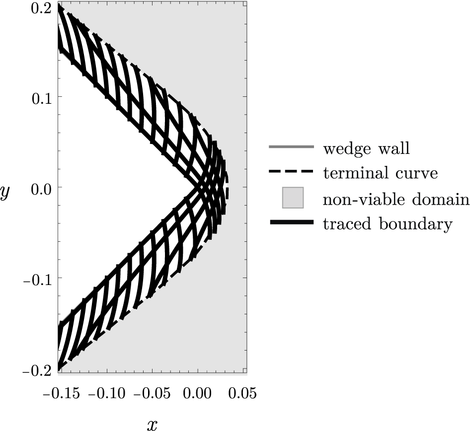
Traced boundaries are computed starting from a range of initial points within the viable domain and using the tracing equations (1.6)–(1.7). Results in the $\gamma = 60^{\circ }$
case are displayed in Figure 6; note the two (positive and negative) branches. To negotiate the corner, one needs to patch together members from both the positive and negative branches near the corner but, although this produces boundaries that negotiate the corner, the resulting boundaries are unsatisfactory because they intercept the boundaries of the viable domain at a finite distance from the corner; we require solutions that asymptote to the wedge face far from the cornerFootnote 2. A suitable modification of the above tracing process does, however, lead to acceptable boundaries, as we now show.
$\gamma = 60^{\circ }$
case are displayed in Figure 6; note the two (positive and negative) branches. To negotiate the corner, one needs to patch together members from both the positive and negative branches near the corner but, although this produces boundaries that negotiate the corner, the resulting boundaries are unsatisfactory because they intercept the boundaries of the viable domain at a finite distance from the corner; we require solutions that asymptote to the wedge face far from the cornerFootnote 2. A suitable modification of the above tracing process does, however, lead to acceptable boundaries, as we now show.


First, note that it is not necessary to use the (prescribed) contact angle $\gamma $
when generating the solution of the Laplace–Young equation to be used for tracing, since the contact angle
$\gamma $
when generating the solution of the Laplace–Young equation to be used for tracing, since the contact angle $\gamma $
does not appear explicitly in the Laplace–Young equation. The solution
$\gamma $
does not appear explicitly in the Laplace–Young equation. The solution $\eta (x,y,\gamma _\bullet )$
corresponding to a different contact angle
$\eta (x,y,\gamma _\bullet )$
corresponding to a different contact angle $\gamma _\bullet $
(the solution contact angle) could equally well be used for generating boundaries, but of course, the domains eventually generated must be such that the prescribed contact angle is
$\gamma _\bullet $
(the solution contact angle) could equally well be used for generating boundaries, but of course, the domains eventually generated must be such that the prescribed contact angle is $\gamma $
around the boundaries. As indicated earlier, the contact surfaces steepen as the boundary wedge is approached, so if one chooses a solution angle
$\gamma $
around the boundaries. As indicated earlier, the contact surfaces steepen as the boundary wedge is approached, so if one chooses a solution angle $\gamma _\bullet <\gamma $
, then there will assuredly be a boundary within the viable domain along which the (prescribed) contact angle is
$\gamma _\bullet <\gamma $
, then there will assuredly be a boundary within the viable domain along which the (prescribed) contact angle is $\gamma $
and, furthermore, such a boundary will asymptote to the wedge walls albeit with an offset (see later). This boundary can be obtained by integrating the tracing equations (1.6)–(1.7) corresponding to the prescribed function
$\gamma $
and, furthermore, such a boundary will asymptote to the wedge walls albeit with an offset (see later). This boundary can be obtained by integrating the tracing equations (1.6)–(1.7) corresponding to the prescribed function $\eta (x,y, \gamma _\bullet )$
and contact angle
$\eta (x,y, \gamma _\bullet )$
and contact angle $\gamma $
; explicitly, the flux function required is given by
$\gamma $
; explicitly, the flux function required is given by
 $$ \begin{align*} F=\cos\gamma \sqrt{1 + (\boldsymbol{\nabla} \eta(x, y, \gamma_\bullet))^2}, \end{align*} $$
with the viability function given by
 $$ \begin{align*} \varPhi= \sin^2\gamma (\boldsymbol{\nabla} \eta(x, y, \gamma_\bullet)^2 - \cot^2\gamma). \end{align*} $$
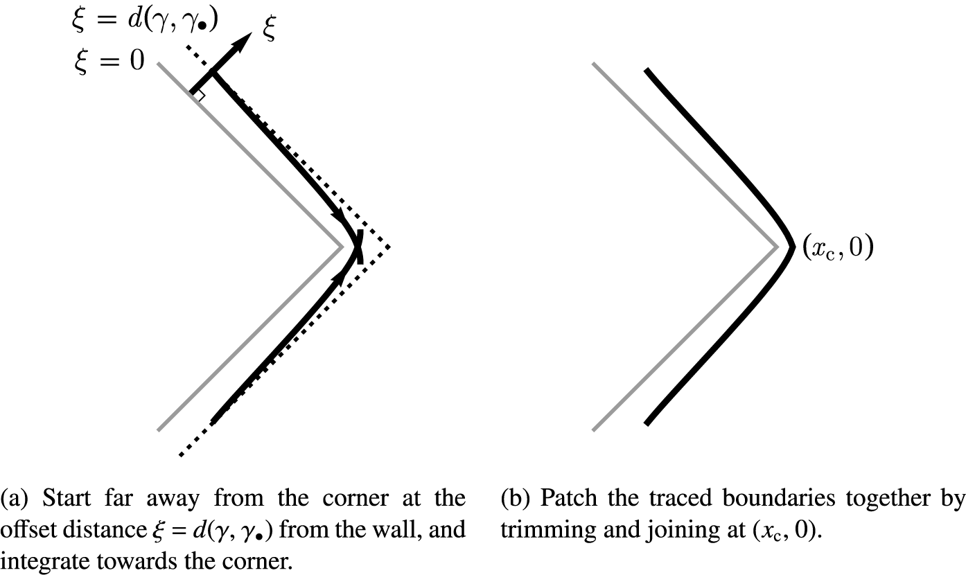
Two such boundary traces, one from each branch, are displayed in Figure 7. By patching together and trimming these traces along the line of symmetry $(x_c,0)$
, we obtain a boundary along which the contact angle is
$(x_c,0)$
, we obtain a boundary along which the contact angle is $\gamma $
. These boundaries asymptote to the wedge angles at large distances from the corner, but with an offset
$\gamma $
. These boundaries asymptote to the wedge angles at large distances from the corner, but with an offset $\xi =d(\gamma , \gamma _\bullet )$
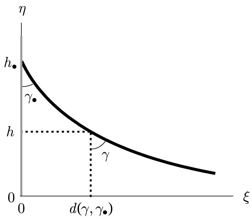
as shown in Figure 7. This offset is determined from the plane wall solution (1.1), shown in Figure 8, and is given by
$\xi =d(\gamma , \gamma _\bullet )$
as shown in Figure 7. This offset is determined from the plane wall solution (1.1), shown in Figure 8, and is given by
 $$ \begin{align} \xi= d (\gamma, \gamma_\bullet) = \cosh^{-1} \bigg({\frac{2}{h_\gamma}}\bigg) - \sqrt{4 - {h_\gamma}^2} - \cosh^{-1} \bigg({\frac{2}{h_{\bullet} }}\bigg) + \sqrt{4 - h_{\bullet} ^2}, \end{align} $$
where
 $$ \begin{align*} h_{\gamma} = \sqrt{2 (1 - \sin\gamma}), \quad h_\bullet = \sqrt{2 (1 - \sin\gamma_\bullet)}. \end{align*} $$
Construction of a corner rounding boundary using a contact angle $\gamma _\bullet < \gamma $
.
$\gamma _\bullet < \gamma $
.

Side view of the half-plane solution (1.3) showing the heights and offset corresponding to $\gamma $
and
$\gamma $
and $\gamma _\bullet $
.
$\gamma _\bullet $
.

This boundary however lies outside the solid wedge and so represents a building up of the solid wedge rather than a rounding, a minor difficulty that can be overcome by sliding the boundary a distance of $\zeta /\sin \alpha $
to the leftFootnote 3. We have thus generated a solution of the Laplace–Young equation with the required contact angle
$\zeta /\sin \alpha $
to the leftFootnote 3. We have thus generated a solution of the Laplace–Young equation with the required contact angle $\gamma $
in a pseudo-rounded corner domain.
$\gamma $
in a pseudo-rounded corner domain.
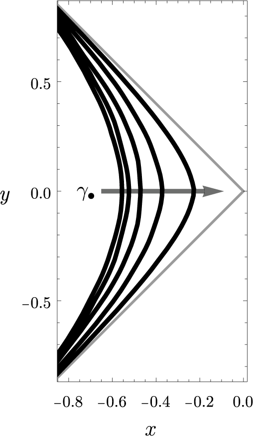
The above process can be repeated for a range of values of $\gamma _{\bullet } <\gamma $
to obtain a one-parameter family of corner pseudo-roundings as displayed in Figure 9. While these “roundings” appear smooth, there is a small slope discontinuity at
$\gamma _{\bullet } <\gamma $
to obtain a one-parameter family of corner pseudo-roundings as displayed in Figure 9. While these “roundings” appear smooth, there is a small slope discontinuity at $(x_c,0)$
. The contact line height corresponding to each of the boundaries is then simply given by evaluating
$(x_c,0)$
. The contact line height corresponding to each of the boundaries is then simply given by evaluating $\eta (r, 3 \pi /4, \gamma _\bullet )$
. Note that all the roundings generated by the above process occur over a distance of the order of the capillary length (unity with the scaling used) and so represent acceptably small geometric modifications. The results are displayed in Figure 10. Of course, all possible roundings of the corner have not been covered using the above approach, but we have obtained results for a representative one-parameter family of corner roundings.
$\eta (r, 3 \pi /4, \gamma _\bullet )$
. Note that all the roundings generated by the above process occur over a distance of the order of the capillary length (unity with the scaling used) and so represent acceptably small geometric modifications. The results are displayed in Figure 10. Of course, all possible roundings of the corner have not been covered using the above approach, but we have obtained results for a representative one-parameter family of corner roundings.
Boundary roundings obtained using contact angles $\gamma _\bullet < \gamma $
with
$\gamma _\bullet < \gamma $
with $\gamma = {60}^{\circ }$
. From left to right:
$\gamma = {60}^{\circ }$
. From left to right: $\gamma _\bullet = {10}^{\circ }, {20}^{\circ }, \ldots , {50}^{\circ }$
.
$\gamma _\bullet = {10}^{\circ }, {20}^{\circ }, \ldots , {50}^{\circ }$
.

Height-rise profiles (parametrized by arc length $s\equiv r$
) corresponding to a contact angle
$s\equiv r$
) corresponding to a contact angle $\gamma = {60}^{\circ }$
: along the original wedge (grey) and along the rounded corner for
$\gamma = {60}^{\circ }$
: along the original wedge (grey) and along the rounded corner for $\gamma _\bullet = {10}^{\circ }, {40}^{\circ }$
(solid black, top to bottom along
$\gamma _\bullet = {10}^{\circ }, {40}^{\circ }$
(solid black, top to bottom along $s = 0$
). The wall height (2.3) (dotted) is shown for reference. Note the exaggerated vertical scale.
$s = 0$
). The wall height (2.3) (dotted) is shown for reference. Note the exaggerated vertical scale.

It is evident from Figure 10 that such corner roundings reduce the step-size of the slope discontinuity at the corner, but only marginally reduce the amount of arching of the contact line; hence, corner rounding fails to produce an acceptable result.
3 Corner rounding with surface roughening
A possible alternative approach to levelling the contact line is to roughen the faces of the solid wedge, with or without corner rounding. Again, we use the numerically generated Laplace–Young solution $\eta (x, y, \gamma _\bullet )$
corresponding to a contact angle
$\eta (x, y, \gamma _\bullet )$
corresponding to a contact angle ${\gamma _\bullet < \gamma }$
to generate new boundaries with the contact angle
${\gamma _\bullet < \gamma }$
to generate new boundaries with the contact angle $\gamma $
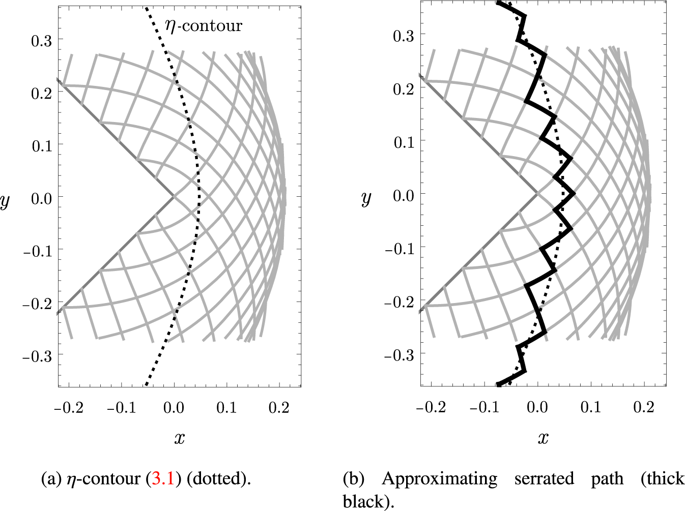
of specific interest, see Figure 11(a).
$\gamma $
of specific interest, see Figure 11(a).
Approximation of an $\eta (x,y, \gamma _\bullet )$
-contour obtained by patching together traced boundaries corresponding to a contact angle
$\eta (x,y, \gamma _\bullet )$
-contour obtained by patching together traced boundaries corresponding to a contact angle $\gamma $
(grey) for
$\gamma $
(grey) for $\gamma _\bullet = {20}^{\circ }$
,
$\gamma _\bullet = {20}^{\circ }$
, $\gamma = {55}^{\circ }$
.
$\gamma = {55}^{\circ }$
.

The two branches of traced boundaries corresponding to the contact angle $\gamma $
form a network as shown. Also plotted in this figure is the
$\gamma $
form a network as shown. Also plotted in this figure is the $\eta $
-contour
$\eta $
-contour
 $$ \begin{align} \eta (x, y, \gamma_\bullet)= h_{\gamma}, \end{align} $$
where $h_{\gamma } $
is the half-plane wall height for the contact angleFootnote 4
$h_{\gamma } $
is the half-plane wall height for the contact angleFootnote 4 $\gamma $
, see (1.4). This contour will asymptote to the wedge walls far from the corner with an offset
$\gamma $
, see (1.4). This contour will asymptote to the wedge walls far from the corner with an offset $d(\gamma , \gamma _\bullet )$
which can be simply corrected for as in the previous section.
$d(\gamma , \gamma _\bullet )$
which can be simply corrected for as in the previous section.
It would be nice for this $\eta $
-contour to be a rounding of the corner, achieving as it does a completely uniform height rise of
$\eta $
-contour to be a rounding of the corner, achieving as it does a completely uniform height rise of $h_{\gamma }$
; however, the
$h_{\gamma }$
; however, the $\eta $
-contour is not a traced boundary, so the contact angle along this curve is not
$\eta $
-contour is not a traced boundary, so the contact angle along this curve is not $\gamma $
as required. Observe, however, that the
$\gamma $
as required. Observe, however, that the $\eta $
-contour may be approximated by a serrated path made from traced boundary portions (with contact angle
$\eta $
-contour may be approximated by a serrated path made from traced boundary portions (with contact angle $\gamma $
) as shown in Figure 11(b), so taking the region to the right of the serrated path as interior, we obtain a new domain with contact angle
$\gamma $
) as shown in Figure 11(b), so taking the region to the right of the serrated path as interior, we obtain a new domain with contact angle $\gamma $
along its boundary and for which the height-rise profile is almost uniform with height
$\gamma $
along its boundary and for which the height-rise profile is almost uniform with height $h_{\gamma }$
. Furthermore, the finer the serrations, the closer the
$h_{\gamma }$
. Furthermore, the finer the serrations, the closer the $\eta $
profile will be to being completely level, see later. This serrated path can be computed from our above results and determines (in the limit) a boundary shape that levels the contact line. However, the result is not practically useful, let alone elegant. Physically, this serrated path may be thought of as a roughened version of the
$\eta $
profile will be to being completely level, see later. This serrated path can be computed from our above results and determines (in the limit) a boundary shape that levels the contact line. However, the result is not practically useful, let alone elegant. Physically, this serrated path may be thought of as a roughened version of the $\eta (x,y,\gamma _\bullet )$
-contour (3.1); we use this observation to obtain a better result.
$\eta (x,y,\gamma _\bullet )$
-contour (3.1); we use this observation to obtain a better result.
The use of small-scale indentations to model roughness in a capillary context is not without precedent. Pioneering work by Wenzel [Reference Wenzel16] noted that a rough surface has a greater surface area than its perfectly smooth counterpart, so that the effective contact angle and the true contact angle have a cosine ratio equal to “the roughness factor”
 $$ \begin{align*} \rho = \frac{\text{Actual surface area}}{\text{Smooth surface area}}. \end{align*} $$
In addition, Anderson et al. [Reference Anderson1, Section 6.4, Reference Anderson, Bassom and Fowkes2] patched together traced boundaries arising from the half-plane solution of the Laplace–Young equation to obtain exact solutions for a multitude of walls with (large and) small indentations. He thus obtained Wenzel’s cosine result independentlyFootnote 5 and provided some numerical verification in the case of sinusoidal indentations.
We repeat here the derivation of Anderson [Reference Anderson1, Section 6.4.2], but adapted to the current context in which we are approximating the $\eta $
-contour (3.1) with a serrated path of traced boundaries as in Figure 11(b).
$\eta $
-contour (3.1) with a serrated path of traced boundaries as in Figure 11(b).
Our aim is to replace the geometrically complex solution (the serrated path with the contact condition (3.4)) with an equivalent homogenized solution (the smooth $\eta $
-contour with “effective” contact angle
$\eta $
-contour with “effective” contact angle $\gamma _{\mathrm {e}}$
).
$\gamma _{\mathrm {e}}$
).
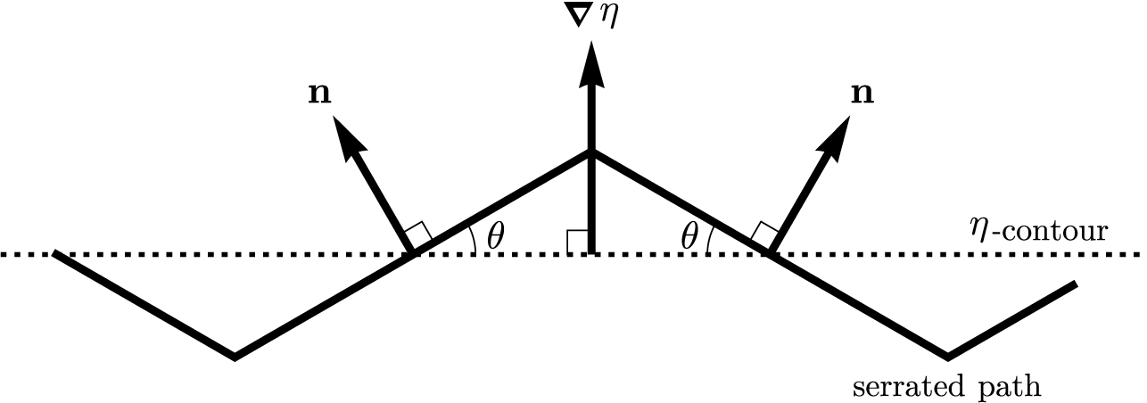
For small enough serrations, both the serrations and the $\eta $
-contour may locally be approximated as straight lines (Figure 12). Since the serrated path is constructed from traced boundaries with a tracing contact angle of
$\eta $
-contour may locally be approximated as straight lines (Figure 12). Since the serrated path is constructed from traced boundaries with a tracing contact angle of $\gamma $
, we have the contact condition
$\gamma $
, we have the contact condition
 $$ \begin{align} {\mathbf{n}} \boldsymbol{\cdot} \frac{\boldsymbol{\nabla} \eta}{\sqrt{1 + (\boldsymbol{\nabla} \eta)^2}} = \cos\gamma \end{align} $$
along the serrated path or, equivalently,
 $$ \begin{align} \frac{|\boldsymbol{\nabla} \eta| \cos\theta}{\sqrt{1 + (\boldsymbol{\nabla} \eta)^2}} = \cos\gamma, \end{align} $$
where $\theta $
is the angle between
$\theta $
is the angle between $ {\mathbf {n}}$
and
$ {\mathbf {n}}$
and $\boldsymbol {\nabla } \eta $
(Figure 12).
$\boldsymbol {\nabla } \eta $
(Figure 12).
Local geometry of the approximation of an $\eta $
-contour with a serrated traced boundary path.
$\eta $
-contour with a serrated traced boundary path.

Now, writing ${\mathbf {n}}_{\mathrm {e}}$
for the normal to the
${\mathbf {n}}_{\mathrm {e}}$
for the normal to the $\eta $
-contour, we have the effective global contact condition given by
$\eta $
-contour, we have the effective global contact condition given by
 $$ \begin{align*} {\mathbf{n}}_{\mathrm{e}} \boldsymbol{\cdot} \frac{\boldsymbol{\nabla} \eta}{\sqrt{1 + (\boldsymbol{\nabla} \eta)^2}} = \cos\gamma_{\mathrm{e}} \end{align*} $$
along the $\eta $
-contour, so that
$\eta $
-contour, so that
 $$ \begin{align} \frac{|\boldsymbol{\nabla} \eta|}{\sqrt{1 + (\boldsymbol{\nabla} \eta)^2}} = \cos\gamma_{\mathrm{e}}, \end{align} $$
since ${\mathbf {n}}_{\mathrm {e}}$
is a unit vector parallel to
${\mathbf {n}}_{\mathrm {e}}$
is a unit vector parallel to $\boldsymbol {\nabla } \eta $
.
$\boldsymbol {\nabla } \eta $
.
The local (3.2) and global (3.4) contact conditions thus match up if
 $$ \begin{align*} \cos \theta= \frac{\cos \gamma}{\cos \gamma_e}.\end{align*} $$
Now, from the geometry of Figure 12, we see that
 $$ \begin{align*} \frac{\text{Serrated path length}}{\text{Contour path length}} = \frac{1}{\cos\theta}, \end{align*} $$
but the length ratio equates to the area ratio $\rho $
for our planar surfaces, so we get
$\rho $
for our planar surfaces, so we get
 $$ \begin{align} \rho = \frac{1}{\cos\theta} = \frac{\cos\gamma_{\mathrm{e}}}{\cos\gamma}, \end{align} $$
thus, the effective contact angle is given by
 $$ \begin{align*} \gamma_{\mathrm{e}} = \cos^{-1} ({\rho \cos\gamma}), \end{align*} $$
which is the Wenzel result.
Note that the roughness factor is always greater than or equal to unity; a perfectly smooth boundary has $\rho = 1$
, a rough boundary has
$\rho = 1$
, a rough boundary has $\rho> 1$
.
$\rho> 1$
.
We now apply these theoretical results to the dip-coating problem. The desired flat coating profile can be achieved as follows.
-
(1) Round the corner of the dipped object in the shape of the $\eta $
-contour (3.1).
$\eta $
-contour (3.1). -
(2) Apply roughness consistent with a serrated path constructed from traced boundaries. From (3.3) and the first equality in (3.5), we see that the required amount of roughness along the
$\eta $
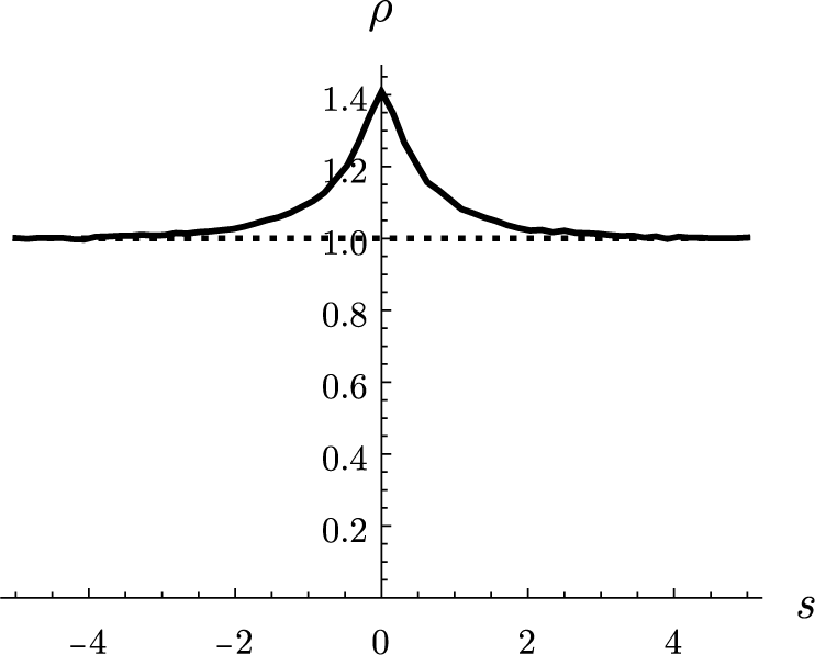
-contour is (3.6)This is a function of position (Figure 13); greater roughness is required near the wedge corner to counteract the natural dip in the height-rise profile for a rounded re-entrant corner. Also note that the roughness coefficient asymptotes to unity over a length of approximately 2. The implication is that surface roughening is only needed over a distance of approximately two capillary lengths from the corner.
$$ \begin{align} \rho = \frac{|\boldsymbol{\nabla} \eta|}{\cos\gamma \sqrt{1 + (\boldsymbol{\nabla} \eta)^2}}. \end{align} $$


If, in Step 3, roughness is applied precisely according to the serrations mandated by boundary tracing, then the theory guarantees that the resulting height-rise profile will be uniform and equal to $h_{\gamma }$
(aside from fine-scale, small-amplitude indentations which disappear in the limit).
$h_{\gamma }$
(aside from fine-scale, small-amplitude indentations which disappear in the limit).
3.1 Indentations: practical implementation
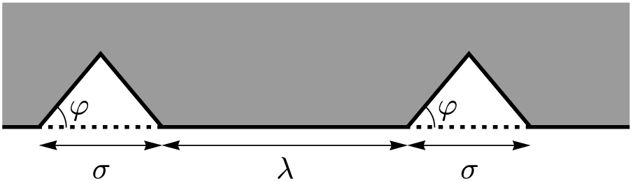
In practice, irregular serrations are difficult and expensive to produce. The theory of Wenzel [Reference Wenzel16] and the computational work of Anderson [Reference Anderson1, Section 6.4.5] indicate that the exact shape of the serrations does not matter as long as the resulting path has the same roughness factor. Therefore, a more practical way of achieving a flat coating profile is to etch regular grooves, with the spacing varied such that the resulting boundary has roughness profile (3.6). For example, consider triangular grooves of constant width $\sigma $
making a constant angle
$\sigma $
making a constant angle $\varphi $
with the
$\varphi $
with the $\eta $
-contour, spaced apart by the variable length
$\eta $
-contour, spaced apart by the variable length $\lambda $
as in Figure 14. The local ratio between the etched path length and the smooth path length is
$\lambda $
as in Figure 14. The local ratio between the etched path length and the smooth path length is
 $$ \begin{align*} \rho = \frac{\sigma / {\cos\varphi} + \lambda}{\sigma + \lambda}; \end{align*} $$
therefore, the grooves should be separated by the distance
 $$ \begin{align*} \lambda = \left({\frac{1 / {\cos\varphi} - \rho}{\rho - 1}}\right) \sigma. \end{align*} $$
Note that the groove angle $\varphi $
cannot be arbitrarily small or large. Let
$\varphi $
cannot be arbitrarily small or large. Let $\rho _0$
be the maximum value of the required roughness (3.6) along the
$\rho _0$
be the maximum value of the required roughness (3.6) along the $\eta $
-contour. At the lower end, we require
$\eta $
-contour. At the lower end, we require $\varphi \ge \cos ^{-1} (1 / \rho _0)$
; we must (at the very least) be able to achieve the maximum required roughness if the grooves are packed at full density (i.e. zero spacing,
$\varphi \ge \cos ^{-1} (1 / \rho _0)$
; we must (at the very least) be able to achieve the maximum required roughness if the grooves are packed at full density (i.e. zero spacing, $\lambda = 0$
). At the upper end, we ought to have
$\lambda = 0$
). At the upper end, we ought to have $\varphi < \gamma $
; each groove is a wedge with half-angle
$\varphi < \gamma $
; each groove is a wedge with half-angle $\pi /2 - \varphi $
, and to avoid the infinite height rise of the small wedge regime and the infinite corner slope of the borderline case, we need
$\pi /2 - \varphi $
, and to avoid the infinite height rise of the small wedge regime and the infinite corner slope of the borderline case, we need $\pi /2 - \varphi> \pi /2 - \gamma $
.
$\pi /2 - \varphi> \pi /2 - \gamma $
.
Triangular grooves of constant width $\sigma $
and constant angle
$\sigma $
and constant angle $\varphi $
, with variable spacing
$\varphi $
, with variable spacing $\lambda $
.
$\lambda $
.

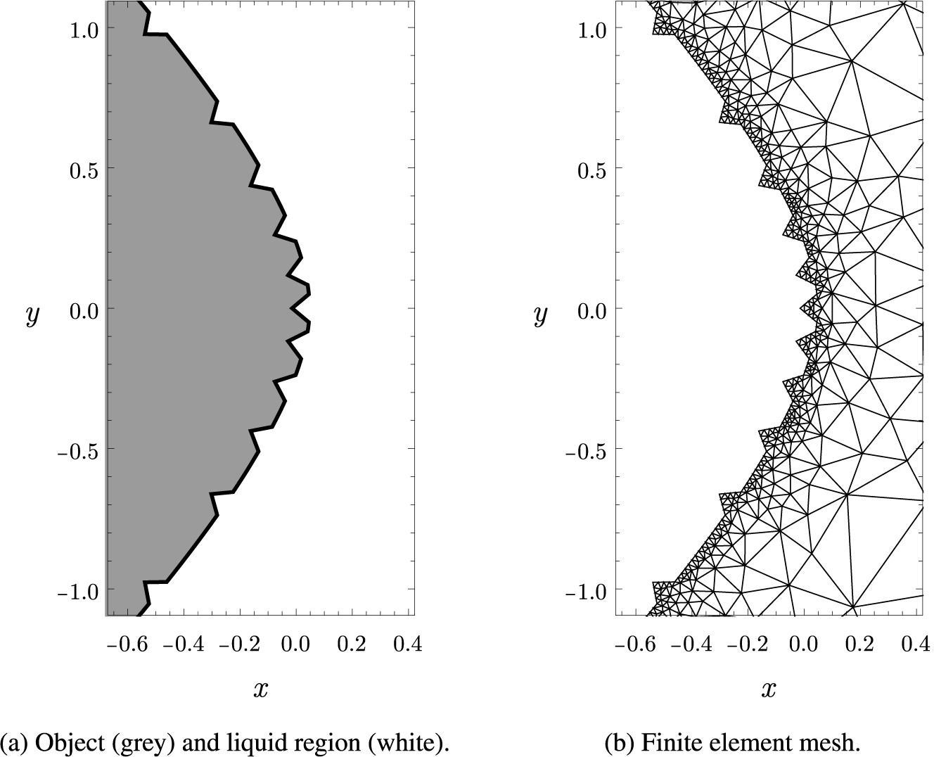
Figure 15(a) shows an example of a groove distribution which approximately achieves the roughness profile of Figure 13. The groove spacing is smaller (and the density higher) near the centre where more roughness is required.


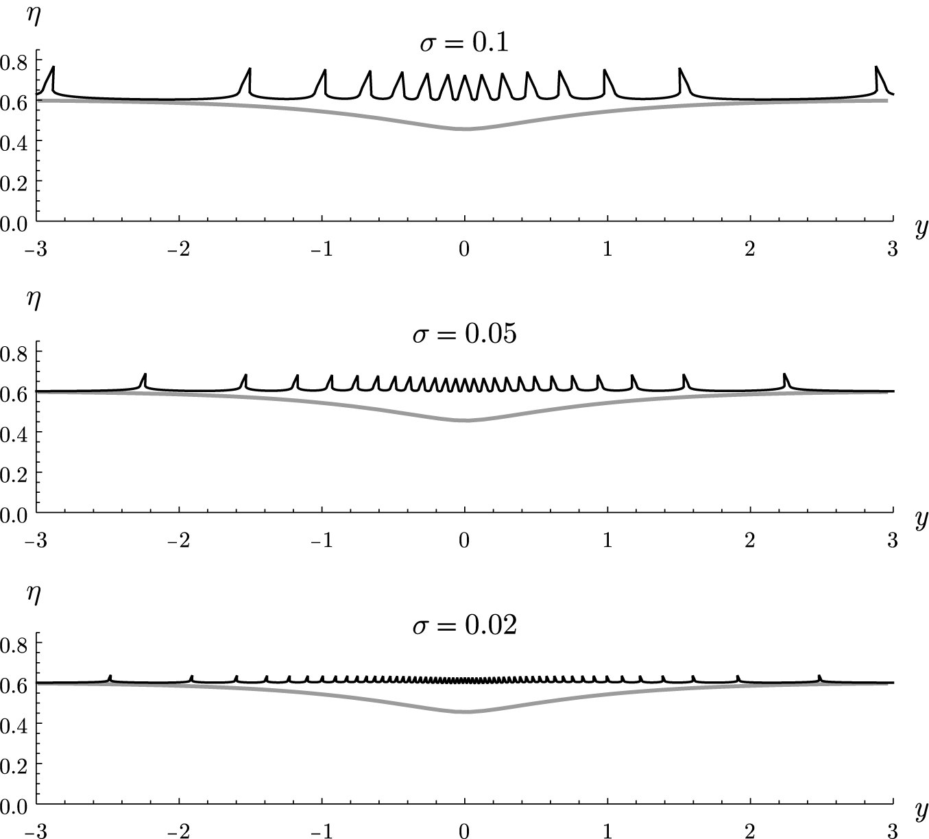
The proposed method of etching regular grooves at variable spacing can be verified numerically. The region occupied by the liquid is discretized as in Figure 15(b) using a minimalistic refinement strategy with fine length scale $\ell = \sigma / 5$
along the grooved boundary to ensure that there is sufficient refinement in the grooves (which have width
$\ell = \sigma / 5$
along the grooved boundary to ensure that there is sufficient refinement in the grooves (which have width $\sigma $
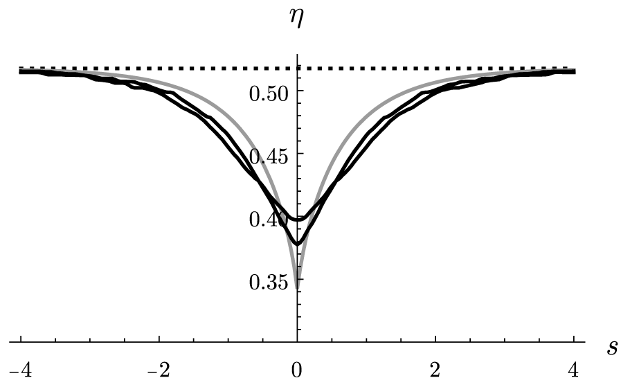
). The capillary BVP (A.1)–(A.2) is then solved. The resulting height-rise profiles are shown in Figure 16. Indeed, the profiles are level with height (3.1) except at the grooves themselves; this is because each groove is itself a moderate wedge admitting a locally planar height rise. Therefore, the height-rise profiles deviate from complete levelness in the form of spikes with height of order
$\sigma $
). The capillary BVP (A.1)–(A.2) is then solved. The resulting height-rise profiles are shown in Figure 16. Indeed, the profiles are level with height (3.1) except at the grooves themselves; this is because each groove is itself a moderate wedge admitting a locally planar height rise. Therefore, the height-rise profiles deviate from complete levelness in the form of spikes with height of order $\sigma $
(the groove width). At this point, it is only a matter of how small the grooves can be made. If infinitesimal grooves were possible, then the deviations from the level height (3.1) would be vanishingly small, but, in practice, the groove width is always nonzero, resulting in spikes with height rise of the same order. Yet also in practice, the wedge corner of an etched groove will not be perfectly sharp; thus, in reality, the observed spikes would be strictly shorter than those in Figure 16.
$\sigma $
(the groove width). At this point, it is only a matter of how small the grooves can be made. If infinitesimal grooves were possible, then the deviations from the level height (3.1) would be vanishingly small, but, in practice, the groove width is always nonzero, resulting in spikes with height rise of the same order. Yet also in practice, the wedge corner of an etched groove will not be perfectly sharp; thus, in reality, the observed spikes would be strictly shorter than those in Figure 16.
Height-rise profiles (parametrized by y) for $\gamma _\bullet = {20}^{\circ }$
and
$\gamma _\bullet = {20}^{\circ }$
and $\gamma = {55}^{\circ }$
, for an object rounded in the shape of the
$\gamma = {55}^{\circ }$
, for an object rounded in the shape of the $\eta $
-contour (3.1), with appropriately positioned grooves of width
$\eta $
-contour (3.1), with appropriately positioned grooves of width $\sigma $
(black) and without grooves (grey). Note the exaggerated vertical scale.
$\sigma $
(black) and without grooves (grey). Note the exaggerated vertical scale.

It should be noted that grooves are not required beyond a distance of approximately two capillary lengths away from the corner, so in the capacitor context, it is simply a matter of applying the above rounding and roughening to each of the corners.
Finally, the result (3.5) asserts that the application of roughness is equivalent to a change in the effective contact angle. Thus, instead of etching grooves into the $\eta $
-contour (3.1), an alternative way to achieve a flat height-rise profile is to modify the contact angle of the dipped object; from (3.4), we see that the required contact angle is given by
$\eta $
-contour (3.1), an alternative way to achieve a flat height-rise profile is to modify the contact angle of the dipped object; from (3.4), we see that the required contact angle is given by
 $$ \begin{align} \gamma_{\mathrm{e}} = \cos^{-1} \left({\frac{|\boldsymbol{\nabla} \eta|}{\sqrt{1 + (\boldsymbol{\nabla} \eta)^2}}}\right), \end{align} $$
a function of position. It is conceivable that the local contact angle of an object could be modified by, for instance, doping it with impurities. Whether this is actually feasible in the specific dipping context and how one might achieve a prescribed dependence on position are questions which we shall leave to the physicists and engineers; however, we note that contact angle modification will produce a much more aesthetically pleasing result than etched grooves in the dipped object.
4 Conclusions
We have shown that a near-level dip-coating profile can be produced by first rounding a re-entrant corner in a prescribed way and then applying a position-dependent amount of roughness. This result is theoretically “exact” in the sense that the curves defining the indentations are exactly determined by the tracing equations in terms of a prescribed solution of the Laplace–Young equation $\eta (x,y, \gamma _\bullet )$
in a wedge; this solution, however, needs to be determined numerically. This roughness can be realized through the etching of regular grooves at a prescribed variable spacing. Of course with three-dimensional printing, this is possible on a small production scale, but clever engineering would be required for commercial production. We have noted that a level dip-coating profile can also be achieved without applying indentations by modifying the contact angle of the dipped object to depend on position in accordance with the effective contact angle (3.7). This would require the careful application of a coating on the surface.
$\eta (x,y, \gamma _\bullet )$
in a wedge; this solution, however, needs to be determined numerically. This roughness can be realized through the etching of regular grooves at a prescribed variable spacing. Of course with three-dimensional printing, this is possible on a small production scale, but clever engineering would be required for commercial production. We have noted that a level dip-coating profile can also be achieved without applying indentations by modifying the contact angle of the dipped object to depend on position in accordance with the effective contact angle (3.7). This would require the careful application of a coating on the surface.
The above results were obtained using the boundary tracing technique, which has the advantage of working with functions defined exactly in terms of the unique solution of the Laplace–Young equation in a $3 \pi /2$
wedge. These functions are solutions of the tracing equations, which are regular first-order ordinary differential equations with unique solutions. In this sense, the results are exact even though
$3 \pi /2$
wedge. These functions are solutions of the tracing equations, which are regular first-order ordinary differential equations with unique solutions. In this sense, the results are exact even though $\eta $
needs to be determined numerically; there is no doubt that the prescribed rounding and roughening results in a level contact line in a limiting sense and we have displayed that good results are obtained for finite indentations.
$\eta $
needs to be determined numerically; there is no doubt that the prescribed rounding and roughening results in a level contact line in a limiting sense and we have displayed that good results are obtained for finite indentations.
The disadvantage of the tracing technique is that by restricting the function set as we have done, we have perhaps not identified other possible boundary modifications that may also result in a level contact line.
Appendix A Numerical solutions in the wedge
To numerically compute the wedge solution using the finite element package in Mathematica, we note that the capillary BVP (1.1) and (1.5) may be viewed as the steady-state diffusion problem
 $$ \begin{align} \boldsymbol{\nabla} \boldsymbol{\cdot} [{K (\boldsymbol{\nabla} \eta) \boldsymbol{\nabla} \eta}] &= \eta, \end{align} $$
 $$ \begin{align} {\mathbf{n}} \boldsymbol{\cdot} [{K (\boldsymbol{\nabla} \eta) \boldsymbol{\nabla} \eta}] &= \cos\gamma, \end{align} $$
with interior sink $\eta $
, boundary supply
$\eta $
, boundary supply $\cos \gamma $
and nonlinear diffusion coefficient
$\cos \gamma $
and nonlinear diffusion coefficient
 $$ \begin{align*} K (\boldsymbol{\nabla} \eta) = \frac{1}{\sqrt{1 + (\boldsymbol{\nabla} \eta)^2}}. \end{align*} $$
Mathematica 12’s NDSolve`FEM´ package has built-in support for solving nonlinear BVPs. When supplied with a nonlinear problem, the built-in function NDSolveValue iteratively solves a linearized version according to Newton’s method. We found that the default initial guess of the zero function is sufficient for achieving convergence.
To approximate an infinite wedge, the domain was taken to be the sector $0 < r < 10$
,
$0 < r < 10$
, $-\alpha < \varTheta < \alpha $
in polar coordinates. The contact condition (A.2) was applied along the two wedge walls
$-\alpha < \varTheta < \alpha $
in polar coordinates. The contact condition (A.2) was applied along the two wedge walls $\varTheta = \pm \alpha $
, and to approximate a vanishing height rise at infinity, the nonwetting zero-flux condition, given by
$\varTheta = \pm \alpha $
, and to approximate a vanishing height rise at infinity, the nonwetting zero-flux condition, given by
 $$ \begin{align*} {\mathbf{n}} \boldsymbol{\cdot} [{K (\boldsymbol{\nabla} \eta) \boldsymbol{\nabla} \eta}] = 0, \end{align*} $$
was applied along the arc $r = 10$
. The domain was discretized into an unstructured triangular mesh. Since the aim was to use the resulting numerical wedge solutions for boundary tracing, we needed to be able to evaluate first derivatives accurately; therefore, we required all mesh elements to have no more area than the equilateral triangle of side length
$r = 10$
. The domain was discretized into an unstructured triangular mesh. Since the aim was to use the resulting numerical wedge solutions for boundary tracing, we needed to be able to evaluate first derivatives accurately; therefore, we required all mesh elements to have no more area than the equilateral triangle of side length $0.2$
. The resulting mesh contained approximately 32 000 elements.
$0.2$
. The resulting mesh contained approximately 32 000 elements.
Acknowledgement
C. Li was supported by an Australian Government Research Training Program (RTP) Scholarship and a Bruce and Betty Green Postgraduate Research Top-Up Scholarship.




























 Open access

