


1. Introduction
One of the best known examples of pattern formation in fluid dynamics concerns Rayleigh–Bénard convection in a fluid layer. As the temperature difference across the layer is increased, the geometry of the flow changes from an initial stationary state in which no flow occurs, to a series of more complex flows. At the onset of convection, patterns of rolls, hexagons or squares can be seen, depending on the nature of the fluid properties (e.g. whether the viscosity is temperature-dependent) and the nature of the boundary conditions. As the temperature difference is increased, further changes in the geometry of the flow occur, with the flow ultimately becoming chaotic and time-dependent.
The transition from one flow geometry to another (e.g. from a stationary state to hexagons) involves a loss of symmetry; the system is said to have undergone a spontaneous symmetry-breaking bifurcation. What is remarkable is that much can be understood about the nature of the bifurcation purely from the consideration of the symmetries of the system. This understanding comes from the subset of dynamical systems theory termed equivariant bifurcation theory, and is well covered in textbooks such as Hoyle (Reference Hoyle2006) and Golubitsky & Stewart (Reference Golubitsky and Stewart2002). The language of symmetry is group theory. Each of the symmetry-breaking transitions from one state to another can be described by a state with a certain symmetry group transitioning to a state whose symmetry is a subgroup of the original group.
Crystallographers have long been concerned with transitions between states with different symmetries. Indeed, there is a celebrated theory of phase transitions in crystals due to Landau (Reference Landau1965), which has much in common with equivariant bifurcation theory. Crystallographers have catalogued detailed symmetry information for periodic structures in the famous International Tables for Crystallography (Hahn Reference Hahn2006), which have been supplemented in recent decades by extensive computer databases such as the Bilbao Crystallographic Server (Aroyo et al. Reference Aroyo, Kirov, Capillas, Perez-Mato and Wondratschek2006a,Reference Aroyo, Perez-Mato, Capillas, Kroumova, Ivantchev, Madariaga, Kirov and Wondratschekb).
The aim of the present paper is to demonstrate how the extensive databases on group theory in crystallography can be exploited to understand transitions in fluid layers. While there has already been extensive use of group theory to understand transitions in fluid layers, authors tend to use a bespoke notation for their particular problem. The advantage of crystallographic notation is that it is standardised. Moreover, there is a wealth of group-theoretic information that can be simply looked up, without the need for it to be re-derived for each new problem. The use of crystallographic notation to describe convective transitions was first advocated by McKenzie (Reference McKenzie1988). The present paper is in a sense an extension of that work, and goes further by exploiting the theory of crystallographic layer groups (Wood Reference Wood1964; Litvin & Wike Reference Litvin and Wike1991), which were added to the International Tables only in 2002 (Kopský & Litvin Reference Kopský and Litvin2010).
There is no new theory discussed in this paper: the theoretical ideas are well established and can be found in textbooks. We aim to provide here an informal introduction to the main ideas, and the interested reader can refer to the literature for the detailed theory. One of the main difficulties with this topic is the large amount of technical jargon needed to properly describe the ideas: the topic encompasses fluid dynamics, representation theory, bifurcation theory and crystallography. Additional difficulties arise because different communities use different words for the same concept (e.g. factor group/quotient group, invariant subgroup/normal subgroup, isotropy group/little group/stabiliser). Where possible, we have tried to use the notation of the International Tables for the crystallographic concepts, and the notation of the textbook by Hoyle (Reference Hoyle2006) for equivariant bifurcation theory.
The paper is organised as follows. In § 2, we establish the fundamental symmetries of fluid layers. This is followed by an introduction to the crystallographic layer groups in § 3, and an introduction to symmetry-breaking transitions in § 4. Section 5 introduces the relevant representation theory, and § 6 the relevant bifurcation theory. The theory is then applied to some simple convection problems in § 7. Three appendices provide additional technical details, and three supplements give tables of group theory information, available at https://doi.org/10.1017/jfm.2024.482.
2. The symmetry of fluid layers
We will consider a fluid dynamical problem that takes place in a layer. In terms of symmetry, it is important to distinguish between three different symmetries: (i) the symmetry of the domain; (ii) the symmetry of the fluid dynamical problem (i.e. the domain plus the governing equations and boundary conditions); and (iii) the symmetry of solutions to the problem. Each of these symmetries may be different.
2.1. Domain symmetries
Let us consider first the symmetries of the domain. We have an infinite fluid layer, and will take  $x$ and $y$ as horizontal coordinates, and $z$ as a vertical coordinate. Let $z=0$ denote the mid-plane of the layer, and let $a$ denote the layer thickness. The domain is thus the region bounded by $-a/2 \leqslant z \leqslant a/2$.
A symmetry of the domain is an invertible map that maps points in the domain to other points in the domain. Here, we will consider only distance-preserving symmetries of the domain (isometries) as these will be the ones of relevance to the physical problem. We can translate all points by a horizontal displacement vector  $\boldsymbol {d} = (d_1, d_2, 0)$, with
 \begin{equation} t_{\boldsymbol{d}}: (x, y, z) \rightarrow (x + d_1, y + d_2, z ), \end{equation}
and retain the same domain  $-a/2 \leqslant z \leqslant a/2$. We also retain the same domain if we rotate about a vertical axis by an angle $\theta$,
 \begin{equation} R^\theta_z: (x, y, z) \rightarrow (x \cos \theta - y \sin \theta, x \sin \theta + y \cos \theta, z ), \end{equation}
or reflect in a vertical mirror plane, e.g. with normal  $x$,
$x$,
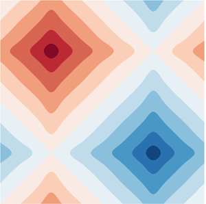
 \begin{equation} m_x: (x, y, z) \rightarrow ( - x, y, z). \end{equation}
The set of all such operations of the form (2.1), (2.2), (2.3) – i.e. all horizontal translations, rotations about vertical axes, and vertical mirrors – and their combinations forms a group known as  $E(2)$, the Euclidean group of distance-preserving transformations in a plane. The fluid layer domain is also invariant under reflections in a horizontal plane, i.e. with normal $z$,
$z$,
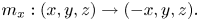
 \begin{equation} m_z: (x, y, z) \rightarrow (x, y, -z), \end{equation}
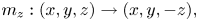
from which it follows that the domain is also invariant under the inversion operation
 \begin{equation} \bar{1}: (x, y, z) \rightarrow ({-}x, -y, -z). \end{equation}
The group of all distance-preserving operations (isometries) of the layer is  $E(2) \times C_2$, a direct product of $E(2)$ and $C_2$, where $C_2$ denotes the cyclic group of order 2 containing two elements (taken here as the identity and the inversion operation). Sometimes, $C_2$ is denoted as $\mathbb {Z}_2$ in other work. The combination of elements in the group $E(2) \times C_2$ leads to operations that are more complex than individual rotations and reflections: e.g. one can have glide reflections that combine a reflection and a translation, and screw displacements that combine translations and rotations.
2.2. Problem symmetries
A fluid dynamical problem in the layer consists of the domain, a set of governing equations and boundary conditions. At each point in the domain, there is a set of field variables that describe the state of the fluid (e.g. its temperature, velocity, pressure). A symmetry operation of the fluid dynamical problem is described by the combination of one of the isometries with a description of how the field variables transform. If the governing equations and boundary conditions are invariant under this transformation, then it is a symmetry of the fluid dynamical problem.
Choices of material properties and boundary conditions mean that not all operations that are isometries of the domain are necessarily symmetries of the fluid dynamical problem. For example, if a different boundary condition is used on the top and bottom of the layer (e.g. fixed temperature on one, fixed flux on another), then the system cannot be invariant under a horizontal mirror such as (2.4). Or if one considers an inclined convection problem where the gravity vector is at an angle to the vertical axis of the layer, then the problem is not invariant under arbitrary rotations about a vertical axis (Reetz, Subramanian & Schneider Reference Reetz, Subramanian and Schneider2020).
A fluid dynamical problem that is invariant under the full group  $E(2) \times C_2$ of isometries of the layer, which will be used in many of the examples which follows, is Rayleigh–Bénard convection in a fluid layer of constant viscosity with appropriately chosen symmetric boundary conditions (e.g. both boundaries being fixed-flux and free-slip) and the Boussinesq approximation. The gravity vector is assumed to be aligned with the vertical. The natural field that describes the state of the system is the temperature. The governing equations are invariant under the operations given in (2.1)–(2.5), provided that the temperature perturbation $\theta$ (the difference in temperature from a conductive steady state) transforms as
 \begin{gather} t_{\boldsymbol{d}}, R_z^\theta, m_x : \theta \rightarrow \theta, \end{gather}
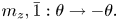 \begin{gather}m_z, \bar{1} : \theta \rightarrow -\theta. \end{gather}
The sign change under horizontal mirror reflection is a manifestation of the symmetry between hot, rising fluid and cold, sinking fluid. A more detailed discussion of the symmetry of this problem can be found in Appendix A.
2.3. Solution symmetries
In general, the symmetries of solutions to the equations are not the same as symmetries of the problem, although the solutions’ symmetries are generically subgroups of the set of symmetries of the problem. Rayleigh–Bénard convection provides a natural example of this: a planform of hexagons or squares is not invariant under any arbitrary translation but only a subgroup of allowed translations. However, one can apply a general element of the symmetry group of the problem to a given solution to yield another solution of the equations.
Figure 1 illustrates the symmetries of a particular solution to Rayleigh–Bénard convection, namely that of convective rolls. Unlike the governing equations, which have a continuous translation symmetry in the  $x$-direction, the rolls have a discrete periodicity. Also unlike the governing equations, the solution is not invariant under a horizontal mirror $m_z$, but it is invariant when the horizontal mirror $m_z$ is combined with a translation by half the width of the unit cell; this is an example of a glide reflection.
An illustration of the symmetries of a simple convective flow, showing a temperature field from a two-dimensional numerical simulation of constant-viscosity Rayleigh–Bénard convection with free-slip, fixed-temperature boundary conditions. This can also be considered as a temperature field in three dimensions for convective rolls if the field is continued into the page (the  $y$-direction). The Rayleigh number is $10^4$, and the flow is steady. The flow pattern is periodic in the $x$-direction, and the repeating unit cell is identified by the thin black lines. Thick black lines indicate vertical mirror planes ( $m_x$). Red ovals indicate twofold horizontal rotation axes ( $2_y$). The red colouring of the oval is used to indicate that the symmetry involves a change of sign of the temperature field (i.e. changing from hot upwelling in red, to cold downwelling in blue). The horizontal dashed red line indicates a horizontal glide plane: the pattern is invariant after translating in the $x$-direction by half the width of the unit cell, reflecting in the horizontal mid-plane, and changing the sign of the temperature field. The rolls in three dimensions also have a continuous translation symmetry in the $y$-direction, and $m_y$ mirrors.
3. Crystallographic layer groups
This work focuses on particular subgroups of  $E(2) \times C_2$ known as the crystallographic layer groups. They are the sets of isometries of the layer that are doubly periodic in space: that is, instead of having continuous translation symmetry in the horizontal as $E(2) \times C_2$ does, the translation symmetry is discrete. The layer groups are invariant under $t_{\boldsymbol {d}}$ in (2.1) only for discrete lattice vectors satisfying
 \begin{equation} \boldsymbol{d} = x \boldsymbol{a}_1 + y \boldsymbol{a}_2, \end{equation}
where  $x, y \in \mathbb {Z}$, and $\boldsymbol {a}_1, \boldsymbol {a}_2$ are basis vectors for the lattice. Many pattern-forming problems lead to steady fluid flows that can be described as having a layer group symmetry. For example, planforms described as squares, hexagons, bimodal, triangles, are all doubly periodic in space and are examples of layer group symmetry. The principal example of a convective flow that is not a layer group symmetry is that of convective rolls: this has a discrete translation symmetry in one horizontal direction, but a continuous translation symmetry in another horizontal direction. Layer groups are an example of a subperiodic group, i.e. a group where the dimension of the space is greater than the dimension of the periodic lattice. For layer groups, the space in which the group elements act is three-dimensional, but there is only a two-dimensional lattice of translations. The layer groups are in a sense intermediate between full three-dimensional space groups (three-dimensional groups with a three-dimensional translation lattice) and the two-dimensional plane or wallpaper groups (two-dimensional groups with a two-dimensional translation lattice).
There are 80 layer groups, and their properties are detailed in the International Tables for Crystallography, volume E (Kopský & Litvin Reference Kopský and Litvin2010) (hereafter referred to as ITE) and in computer databases such as the Bilbao Crystallographic Server (de la Flor et al. Reference de la Flor, Souvignier, Madariaga and Aroyo2021) (hereafter referred to as BCS). Each layer group is identified by a unique number and Hermann–Mauguin (HM) symbol. One example that we will focus on is the layer group  $p4/nmm$ (layer group 64, illustrated in figure 2a). This group has a square lattice, a fourfold vertical rotation axis, two conjugate sets of vertical mirror planes, and a glide reflection $n$ that combines reflection in a horizontal plane with a translation by $(\tfrac {1}{2}, \tfrac {1}{2}, 0)$. The first letter of the Hermann–Mauguin symbol denotes the centring type of the conventional unit cell: for layer groups, this is either $p$ for primitive cell, or $c$ for centred cell. The next one, two or three elements of the symbol describe symmetry elements about different axes. For $p4/nmm$, the three elements are $4/n$, $m$ and $m$. The $4/n$ element denotes the presence of both the fourfold vertical rotation axis and the glide reflection $n$, whose glide plane also has a vertical normal (the slash indicates that the rotational symmetry axis and the normal to the glide plane are parallel). The next two elements labelled $m$ represent vertical mirror planes. Other possible Hermann–Mauguin elements found in other layer group symbols include the symbol $\bar {1}$ representing the inversion operation of (2.5), the symbols $\bar {3}$, $\bar {4}$ and $\bar {6}$ that combine threefold, fourfold or sixfold rotation with an inversion, and $a$ or $b$ for glide reflections with translations parallel to the basis vectors of the lattice $\boldsymbol {a}_1$ and $\boldsymbol {a}_2$, respectively.
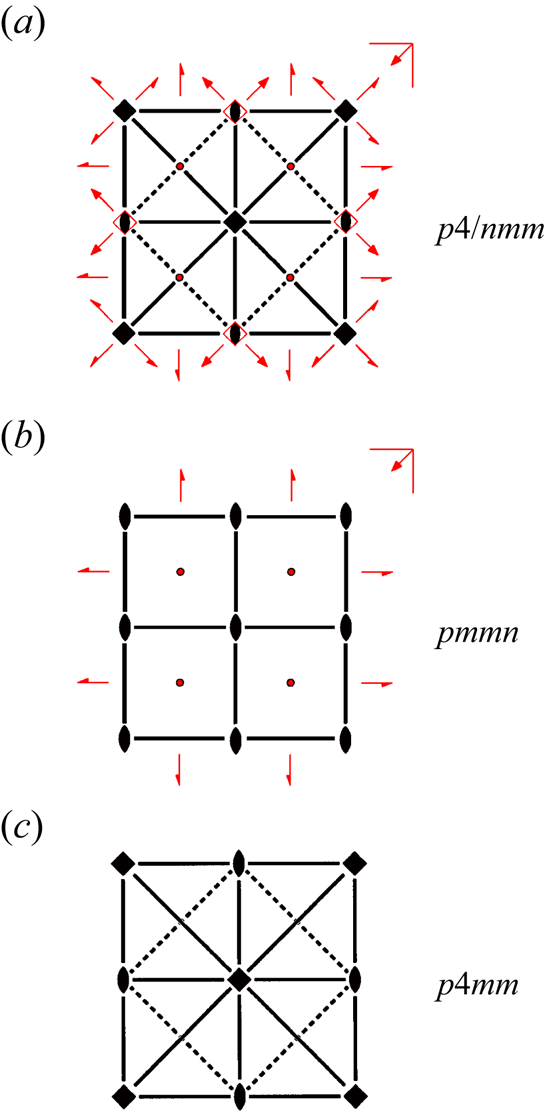
Symmetry diagrams from ITE for (a)  $p4/nmm$ (origin choice 1), and two of its subgroups, (b) $pmmn$ and (c) $p4mm$. Shown here is the unit cell in a projection onto the horizontal mid-plane. Squares indicate fourfold vertical rotation axes ( $4_z$), filled ovals are twofold vertical rotation axes ( $2_z$), circles are inversion centres ( $\bar {1}$), and unfilled squares with filled ovals indicate a $\bar {4}_z$ vertical inversion axis ( $\bar {4}_z$ combines the fourfold vertical rotation $4_z$ with the inversion operation $\bar {1}$). Solid lines are vertical mirror planes, dashed lines are vertical glide planes. The symbol in the top right refers to the horizontal glide plane $n$, where the symmetry operation combines a vertical mirror $m_z$ with a translation by $(\tfrac {1}{2}, \tfrac {1}{2}, 0)$. Full arrows around the edge refer to a horizontal twofold rotation axis; half-arrows refer to a twofold screw axis. Red colouring indicates symmetry operations that send $z \rightarrow -z$ and will be associated with sign changes in the temperature field (hot to cold and vice versa). Examples of convective flows with these symmetries are shown in figures 3(b), 4(b), 6, 7 and 8.
From (2.7), we have that a symmetry operation that sends  $z \rightarrow - z$ involves a change in sign of the temperature perturbation (i.e. hot to cold or vice versa). There is a broader class of crystallographic groups termed ‘black and white’, ‘magnetic’ or ‘Shubnikov’ that have as a possible group element $1^\prime$, which changes the sign of a field without changing position. With such groups, a combination of a horizontal mirror and a sign change would be denoted as $m_z^\prime$, and the black-and-white layer groups depicted in figures 2(a,b) would be referred to as $p4/n^\prime m m$ and $pmmn^\prime$ (Litvin Reference Litvin2013). However, here we will not denote the symmetry operations with primes for two reasons. First, the fluid problems that we consider are invariant only on combining the sign change in $\theta$ with the horizontal mirror; they are not invariant under a sign change in $\theta$ alone, so the $1^\prime$ operator is not present. Second, a general fluid dynamical problem can consist of more field variables that just one, and each variable may transform in a different way under the isometries, e.g. the horizontal velocities and the toroidal potential do not change sign under $m_z$ (see Appendix A). We will simply write $m_z$ as the group element corresponding to horizontal mirror reflection and it should be understood that it acts on different fields in different ways (some change sign, some do not).
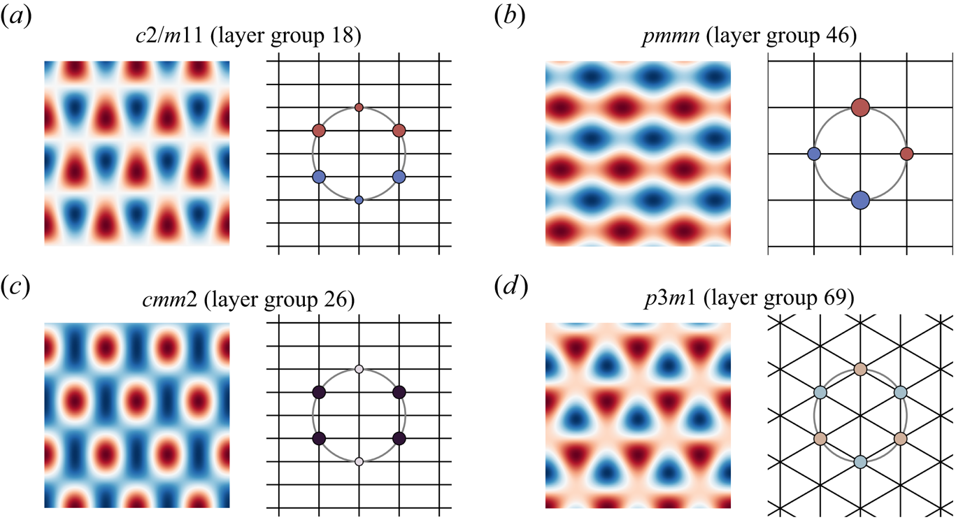
Many of the plots in this paper show the temperature field in the horizontal mid-plane. Position in the mid-plane is invariant under the horizontal mirror  $m_z$; the only action of $m_z$ in the mid-plane is to change the sign of the temperature perturbation. The mid-plane temperature fields can therefore be considered as belonging directly to one of the two-dimensional black-and-white plane groups. There are 80 black-and-white plane groups, which are isomorphic to the 80 layer groups. A mapping between the symbols used for black-and-white plane groups and those for layer groups can be found in ITE.
4. Symmetry-breaking transitions
Suppose that as a control parameter (such as the Rayleigh number) is varied, a symmetry-breaking transition occurs from a state with symmetry group  $G$ to a state with a lower-symmetry group $H$. For simplicity, let us just consider steady states. Purely from symmetry arguments alone there is often much that can be said about the nature of the transition: e.g. one can often classify the nature of the bifurcation as being either pitchfork or transcritical, and also write down the generic form of the equations describing the amplitudes of the critical modes (§ 6). More generally, given an initial state with a group $G$, one can determine the possible groups $H$ that can arise in a symmetry-breaking transition.
The first requirement for  $H$ is that it is a subgroup of $G$. Subgroups of layer groups have a particular structure and classification (Müller Reference Müller2013) where the letters $t$ and $k$ refer to the symmetries that are retained. A subgroup is termed a translationengleiche subgroup or $t$-subgroup if it has the same translation symmetries as its parent. A $t$-subgroup has a different point group to its parent so is necessarily a non-isomorphic subgroup with a different layer group number and symbol. A subgroup is termed a klassengleiche subgroup or $k$-subgroup if the translations are reduced but the order of the point group remains the same. The $k$-subgroups can be further categorised into those that are isotypic (have the same layer group number and symbol) and those that are non-isotypic (have a different layer group symbol). Finally, a subgroup may have both the order of the point group reduced and the translations reduced. However, in this case, there always exists an intermediate subgroup $M$ such that $M$ is a $t$-subgroup of $G$, and $H$ is a $k$-subgroup of $M$ (Hermann's theorem). As such, any subgroup $H$ of $G$ can be described in terms of a chain of $t$ and $k$ relationships.
A subgroup  $H$ of a group $G$ is termed maximal if there is no intermediate subgroup $M$ of $G$ such that $H$ is a proper subgroup of
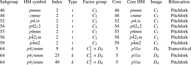
  $M$. Both ITE and the BCS provide comprehensive lists of the maximal subgroups of the layer groups, from which parent group–subgroup relationships can be described. An example of such subgroup information is given in table 1 for the layer group $p4/nmm$, along with additional information useful for describing symmetry-breaking bifurcations. Similar tables for all 80 layer groups can be found in supplement 1. In table 1, each maximal subgroup is listed with its layer group number and Hermann–Mauguin symbol. The index of the subgroup in the parent is given (the index is the number of left cosets of the subgroup in the parent). The type of subgroup is given as either $t$ or $k$ for translationengleiche or klassengleiche. The nature of the additional information in table 1 on factor group, core, and bifurcation is described in §§ 5 and 6.
Maximal subgroups of  $p4/nmm$ (layer group no. 64).
Group theory places more constraints on the group  $H$ than it simply being a subgroup of $G$. In fact, for a generic steady-state symmetry-breaking bifurcation, the subgroup $H$ must be an isotropy subgroup of a particular absolutely irreducible representation of the group $G$ (Golubitsky & Stewart Reference Golubitsky and Stewart2002; Hoyle Reference Hoyle2006). Thus to understand symmetry-breaking bifurcations of layer groups, we must understand their group representations, which we turn to now.
5. Representations of layer groups
A representation of a group is simply a mapping of the group elements to a set of matrices in a way that preserves the group operation (i.e. the mapping is a homomorphism onto  $GL(V)$). A representation acts on a certain vector space $V$ of dimension $n$. An invariant subspace of a representation is a vector subspace $W$ that has the property that $\boldsymbol{\mathsf{D}} \boldsymbol {w} \in W$ for all $\boldsymbol {w} \in W$ and for all $\boldsymbol{\mathsf{D}}$ in the set of representation matrices. The spaces $W=\lbrace \boldsymbol {0} \rbrace$ and $W=V$ are always invariant subspaces, known as the trivial subspaces. If the representation contains a non-trivial invariant subspace, then it is said to be reducible; otherwise, it is irreducible. A representation is absolutely irreducible if the only linear maps that commute with the representation are multiples of the identity. For representations over $\mathbb {C}$, there is no distinction between being absolutely irreducible and just irreducible, but there is a difference over $\mathbb {R}$, where representations can be irreducible but not absolutely irreducible. Irreducible representations (or irreps for short) are the building blocks of representation theory. Any representation of a group can be written as a direct sum of its irreducible representations (Maschke's theorem).
Given a point  $\boldsymbol {v} \in V$, we can define its isotropy subgroup $\varSigma$ as
 \begin{equation} \varSigma= \lbrace { g \in G : g \boldsymbol{v} = \boldsymbol{v}} \rbrace \end{equation}
and its corresponding fixed-point subspace by
 \begin{equation} \operatorname{Fix} (\varSigma) = \lbrace {\boldsymbol{w} \in V : g \boldsymbol{w} = \boldsymbol{w}, \forall g \in \varSigma} \rbrace. \end{equation}
An isotropy subgroup is said to be axial if the dimension of its fixed-point subspace is 1. Axial isotropy subgroups are of particular interest because the existence of solution branches with the given isotropy subgroup is guaranteed under certain conditions by the equivariant branching lemma (Golubitsky & Stewart Reference Golubitsky and Stewart2002; Hoyle Reference Hoyle2006).
Classifying the steady-state symmetry-breaking bifurcations of layer groups consists of identifying their irreducible representations, and subsequently finding their isotropy subgroups. The general theory of irreducible representations of layer groups in detail is somewhat involved, but it is known, and results can simply be looked up in textbooks or extracted from computer databases. In many cases it is not necessary to invoke the full general theory, as the appropriate irreps can be found quickly by lifting from an appropriate factor group.
5.1. Lifting representations
Given a group  $G$ and a normal subgroup $N$, one can form the factor group (or quotient group) $G/N$. The elements of $G/N$ are the left cosets of $N$ in $G$, which have a well-defined multiplication operator when the subgroup $N$ is normal.
Suppose that we are interested in understanding a transition between a group  $G$ and a subgroup $H$. We want to know the irrep of $G$ associated with the transition. In the crystallography literature, this is termed ‘the inverse Landau problem’ (Ascher & Kobayashi Reference Ascher and Kobayashi1977; Litvin, Fuksa & Kopsky Reference Litvin, Fuksa and Kopsky1986). One solution to this is as follows. We first find the normal core $N$ of the subgroup $H$ in $G$, i.e. the largest normal subgroup of $G$ that is contained in $H$. In some cases, this may be the whole subgroup $H$, but not in general. We then form the factor group $G/N$, and we refer to this as the factor group associated with the transition. Table 1 gives the factor groups and normal cores associated with each of the maximal subgroups of $p4/nmm$. The table also gives the image of the subgroup $H$ under the natural homomorphism onto cosets of $N$. The advantage of finding the factor group $G/N$ is that it is typically a small finite group, so finding its irreps is much more straightforward than finding the irreps for the group $G$ (which in the case of layer groups is an infinite group). Moreover, the irreps of the factor group $G/N$ can be lifted to an irrep of the group $G$ using the natural homomorphism onto cosets. Suppose that we have an irrep $\rho$ of the factor group,
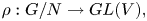 \begin{equation} \rho: G/N \rightarrow GL(V), \end{equation}
and suppose that  $q$ is the natural homomorphism
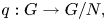 \begin{equation} q : G \rightarrow G/N, \end{equation}
where  $q(g) = g N$. Then the composition $\rho \circ q$ is the irrep of $G$ lifted from $G/N$. Indeed, it is an irrep of $G$ with $N$ in its kernel. Representations lifted from a factor group are sometimes termed engendered representations in the crystallography literature.
All the  $t$-subgroups of $p4/nmm$ have the same factor group, namely $C_2$. In this case, the subgroups are all normal subgroups, so the normal core $N$ is the same as the subgroup $H$. The irreps associated with these transitions are very simple. They are one-dimensional and just send each element of the subgroup $H$ to 1, and all others to $-1$. As will be discussed later, this is associated with a pitchfork bifurcation. Any index-2 subgroup necessarily has a factor group of $C_2$ and is associated with a pitchfork bifurcation.
5.2. The  $t$-subgroups

The irreps associated with translationengleiche transitions, which preserve the translations of the lattice, can be found by lifting from an appropriate factor group. The set of all translations  $T$ of the lattice forms a normal subgroup of any layer group. Therefore the irreps of $G$ with the pure translations in the kernel can be found by lifting from the factor group $G/T$. The factor group $G/T$ is isomorphic to the isogonal point group associated with the layer group, so the irreps are simply those of the corresponding point group.
The character table for the factor group  $G/T$ is shown for $p4/nmm$ in table 2, and is the same as that for isogonal point group $4/mmm$ ( $D_{4h}$). Similar tables for all 80 layer groups can be found in supplement 2. The character of a representation matrix is simply its trace. Characters are independent of the basis used in the representation, and are the same for group elements that are conjugate. A character table simply consists of a table of all the characters for all the irreps of a group. For many applications of representation theory, it is sufficient to know the characters of the representation and it is not necessary to know the representation matrices themselves.
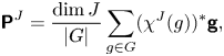
Translationengleiche character table of  $p4/nmm$ (no. 64). The column headings give the Seitz symbol labels for a member of each conjugacy class. The number of elements in each conjugacy class is listed in the first row of the table. Each irrep is given a label on the left using Mulliken notation. The rightmost column gives the corresponding axial isotropy subgroups associated with each irrep. Note that the Seitz symbol labels refer only to the point group part of the symmetry operations; the coset representatives of $2_y$, $2_{xy}$, $\bar {1}$, $m_z$, $\bar {4}_z$ also involve a translation by $(\tfrac {1}{2}, \tfrac {1}{2}, 0)$ (see the ITE description of $p4/nmm$, origin choice 1).
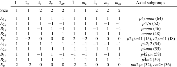
Each of the seven  $t$-subgroups listed in table 1 is associated with one of the one-dimensional irreps in table 2. There are also additional axial subgroups identified in table 2 associated with the two-dimensional representations labelled $E_g$ and $E_u$. These subgroups are not in table 1 as they are not maximal subgroups. It should be stressed that isotropy subgroups need not be maximal subgroups.
5.3. General theory of representations of layer groups
Irreps associated with  $k$-transitions, where translation symmetries are lost, can also be obtained by lifting from appropriate factor groups. An example is given in table 1, which lists an index-9 $k$-transition from $p4/nmm$ to $p4/nmm$ where the associated irreps could be found by considering the irreps of the corresponding factor group $C_3^2 \rtimes D_4$ (where $C_3^2$ denotes the direct product of $C_3$ with itself, i.e. $C_3 \times C_3$, and the symbol $\rtimes$ denotes the semi-direct product). A discussion of the irreps of this particular factor group can be found in Matthews (Reference Matthews2004) (see his figure 1). Such a transition is an example of a spatial-period-multiplying bifurcation where the periodicity of the pattern is broken but maintained on a larger scale: in this case, after the symmetry break, the lattice basis vectors are scaled by a factor 3 in each direction.
An alternative approach is to exploit the general theory that describes the complete set of irreps of layer groups. This theory is somewhat involved, but is understood, and one can simply look up appropriate representations using published tables (Bradley & Cracknell Reference Bradley and Cracknell1972; Litvin & Wike Reference Litvin and Wike1991; Milosevic et al. Reference Milosevic, Nikolic, Damnjanovic and Krcmar1998) or computer software (Aroyo et al. Reference Aroyo, Kirov, Capillas, Perez-Mato and Wondratschek2006a; Stokes, van Orden & Campbell Reference Stokes, van Orden and Campbell2016; de la Flor et al. Reference de la Flor, Souvignier, Madariaga and Aroyo2021).
The starting point for the general theory concerns the representations of the subgroup  $T$ of all translations of the lattice. The subgroup $T$ is a normal subgroup of any layer group. It is also an Abelian group, so its irreps are one-dimensional. The irreps of $T$ are simply $\mathrm {e}^{-\mathrm {i} \boldsymbol {k} \boldsymbol {\cdot } \boldsymbol {d}}$ for a translation by a vector $\boldsymbol {d}$, where $\boldsymbol {k}$ is a wavevector which labels the particular irrep. Wavevectors that differ by a reciprocal lattice vector lead to identical irreps. As such, the wavevectors for defining irreps are restricted to a region of reciprocal space known as the Brillouin zone (a unit cell in reciprocal space) such that each irrep has a unique $\boldsymbol {k}$ label.
The irreps of the layer groups can be built up from the irreps of  $T$ using the theory of induced representations (see Appendix B for a brief example, and Bradley & Cracknell (Reference Bradley and Cracknell1972), Aroyo et al. (Reference Aroyo, Kirov, Capillas, Perez-Mato and Wondratschek2006a) and de la Flor et al. (Reference de la Flor, Souvignier, Madariaga and Aroyo2021) for the detailed theory). Each irrep is labelled by a wavevector $\boldsymbol {k}$, a symbol that represents the type of wavevector (the labels $\varGamma$, $\varSigma$, $\varDelta$, and so on in figure 10 of Appendix B), and an index ( $1, 2, 3,\ldots$) referencing a particular representation of the little group of the wavevector. For example, the index-9 $k$-transition from $p4/nmm$ to $p4/nmm$ is associated with two possible irreps of the parent group: $^* \varSigma _1$ with $\boldsymbol {k} = (1/3, 1/3)$, and $^* \varDelta _3$ with $\boldsymbol {k} = (0, 1/3)$. The full matrices of these representations are given in § B.2. The irreps associated with $t$-transitions have a zero wavevector, $\boldsymbol {k}=(0, 0)$. These are sometimes labelled by $^*\varGamma$ and an index, rather than the Mulliken symbols used in table 2, as they correspond to the $\varGamma$ point in the Brillouin zone (figure 10).
Much information can be obtained about the irreps and isotropy subgroups associated with transitions by querying computer databases (Aroyo et al. Reference Aroyo, Kirov, Capillas, Perez-Mato and Wondratschek2006a; Perez-Mato, Aroyo & Orobengoa Reference Perez-Mato, Aroyo and Orobengoa2012; Stokes et al. Reference Stokes, van Orden and Campbell2016; de la Flor et al. Reference de la Flor, Souvignier, Madariaga and Aroyo2021; Iraola et al. Reference Iraola, Mañes, Bradlyn, Horton, Neupert, Vergniory and Tsirkin2022). Given a parent group and a subgroup, one can ask the software tools to provide the associated irreps and the corresponding fixed-point subspaces of the isotropy subgroups. For a given parent group, one can also obtain from the tools a complete listing of all possible isotropy subgroups and the corresponding irreps. Most of these software tools are designed for use on full three-dimensional space groups, rather than layer groups. However, each layer group can be associated with a corresponding space group (Litvin & Kopský Reference Litvin and Kopský2000). Given a three-dimensional space group  $S$, and $T_z$ as the one-dimensional subgroup of $S$ of the vertical translations, the factor group $S / T_z$ is isomorphic to a layer group. The irreps of layer groups can be obtained from the irreps of space groups where the wavevector is constrained to lie in a particular plane.
6. Equivariant bifurcation theory
Once the irrep associated with a particular transition is known, the nature of the bifurcation can be understood using equivariant bifurcation theory (Hoyle Reference Hoyle2006; Crawford & Knobloch Reference Crawford and Knobloch1991; Golubitsky & Stewart Reference Golubitsky and Stewart2002). The full dynamics, which is described by a set of partial differential equations, can be reduced in the neighbourhood of the bifurcation point to simple ordinary differential equations of the form
 \begin{equation} \frac{\mathrm{d} \boldsymbol{y}}{\mathrm{d} t} = \boldsymbol{f}(\kern 1.5pt \boldsymbol{y}; \mu) \end{equation}
using methods such as centre manifold reduction or Lyapunov–Schmidt reduction. Such equations are termed amplitude equations. Here,  $\boldsymbol {y}$ is the vector of mode amplitudes (which would be referred to as an order parameter in crystallography), and is of the same dimension as the irrep. Also, $\mu$ is the bifurcation parameter, which for convection problems can be related to the Rayleigh number. Bifurcation occurs when $\mu$ passes through zero.
The function  $\boldsymbol {f}(\kern 1.5pt \boldsymbol {y}; \mu )$ is equivariant under the action of the matrices of the given irrep, i.e.
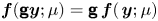 \begin{equation} \boldsymbol{f}( \boldsymbol{\mathsf{g}} \boldsymbol{y}; \mu) = \boldsymbol{\mathsf{g}}\, \boldsymbol{f}(\kern 1.5pt \boldsymbol{y}; \mu ) \end{equation}
for all matrices  $\boldsymbol{\mathsf{g}}$ in the given irrep. Equivariance places strong constraints on the form of the amplitude equations, and in turn on the nature of the bifurcation. Equivariance under a non-trivial irrep implies that $\boldsymbol {f}(\boldsymbol {0}; \mu ) = \boldsymbol {0}$, hence $\boldsymbol {y} = \boldsymbol {0}$ is always an equilibrium solution (although not necessarily a stable one). Steady-state bifurcations without symmetry constraints are generically saddle-node bifurcations; it is the constraints from symmetry that lead to pitchfork or transcritical bifurcations instead.
The simplest example of the consequences of equivariance are in a one-dimensional system, invariant under  $C_2 = \lbrace 1, -1 \rbrace$. Equivariance under $C_2$ implies that the function $f$ is odd ( $\,f(-y; \mu ) = - f(y; \mu )$), which in turn implies that in a Taylor expansion of $f(y; \mu )$ about $y=0$, no even-order terms in $y$ will appear. It follows from the symmetry alone that the associated bifurcation must be a pitchfork.
A common method of analysing amplitude equations is to consider their Taylor expansion in powers of  $\boldsymbol {y}$, and to truncate at some particular order. Much generic behaviour about the bifurcation can be described by these truncated forms. Moreover, symmetry places constraints on the number of independent parameters needed to describe the truncated form: for the $C_2$ example, there are no quadratic or other even-order terms present. The dimension of the space of equivariants of given degree can be obtained purely using the characters of the representation (see Appendix C and Antoneli, Dias & Matthews Reference Antoneli, Dias and Matthews2008). This can be used to show, for example, that the faithful irrep of $D_3$ has a quadratic equivariant, unlike $C_2$. The faithful irrep of $D_3$ is generically associated with a transcritical bifurcation, although for a particular problem there is always the possibility that the coefficient associated with the quadratic equivariant is zero due to some particular feature of the governing equations (e.g. self-adjointness; Golubitsky, Swift & Knobloch Reference Golubitsky, Swift and Knobloch1984) that would then cause the bifurcation to be a pitchfork.
The final column of table 1 classifies the type of generic steady-state bifurcation associated with each of the maximal subgroups of  $p4/nmm$. Only the index-9 $k$-transition is associated with a transcritical bifurcation; all others are pitchforks. The bifurcations can generically be classified depending on whether the dynamics when restricted to the fixed-point subspace has a quadratic term: pitchfork if not, transcritical if so. The classification of bifurcations is discussed further in supplement 3, which provides character tables of several small finite groups and the dimensions of their spaces of equivariants.
7. Convection
We will now apply the theory discussed in the previous sections to transitions in fluid layers, and in particular to thermal convection. Consider a layer of fluid, heated from below and cooled from above. As the Rayleigh number is increased past some critical value, the system begins to convect. Depending on choices of boundary conditions and rheology, different planforms of the flow are possible: common planforms seen at onset are rolls, hexagons and squares. Each of these convective planforms can be classified using crystallographic notation, e.g. squares have layer group symmetry  $p4/nmm$ (layer group 64), as illustrated in figure 3(b).
Examples of crystallographic classification for convective flows consisting of a single horizontal wavenumber: (a) rolls, (b) squares (checkerboard), (c) rectangles (patchwork quilt), (d) triangles, (e) down-hexagons, (f) anti-squares, (g) anti-hexagons. Each pattern, with the exception of rolls, is labelled by its Hermann–Mauguin layer group symbol. The pattern of rolls does not correspond to a layer group, as it has one axis with a continuous translation symmetry (its symmetry may be referred to as  $\mathcal {p}_a {\nu }_b ma2$; Kopský Reference Kopský2006). The left-hand plot of each panel shows the mid-plane temperature field; the right-hand plot shows its Fourier transform (reciprocal space plot). In reciprocal space, the size of the dots shows the amplitude, the colour of the dots shows the phase (colour bar in top right). Grid lines indicate the reciprocal lattice, although note that some mode patterns are consistent with more than one type of lattice (e.g. both hexagonal and rectangular). The lattice shown is that used in ITE for the given layer group. With a single horizontal wavenumber, all modes must lie on a circle in reciprocal space (grey line). All of these patterns represent a single-parameter family: once the origin and orientation is specified, the only remaining parameter is the amplitude.

The physical state of the fluid can be described by its temperature field. Figure 3 shows examples of possible temperature fields that can occur at the initial onset of convection. Each panel shows the mid-plane temperature field with red/blue colouring for hot/cold, along with the corresponding reciprocal space (Fourier domain) pattern, where each dot is coloured according to phase, and the size of the dot indicates its amplitude. At the onset of convection, there is typically a single critical horizontal wavenumber  $k_c$, and the horizontal variation is described by a planform function $f(x,y)$ satisfying $\boldsymbol {\nabla }_h^2\, f = - k_c^2 f$ (Ribe Reference Ribe2018). When constrained to a periodic lattice, the planform function is a superposition of modes of the form $\exp ({{\rm i} (k_x x + k_y y)})$, where $\boldsymbol {k} = (k_x, k_y)$ is the horizontal wavenumber vector, and $|\boldsymbol {k}|=k_c$. Thus in the reciprocal space plots of figure 3, all the dots lie on a circle of radius $k_c$.
Figures 3(f,g) show examples of superlattice patterns (Dionne, Silber & Skeldon Reference Dionne, Silber and Skeldon1997; Dawes, Matthews & Rucklidge Reference Dawes, Matthews and Rucklidge2003; Hoyle Reference Hoyle2006). These are patterns where the critical wavenumber  $k_c$ is larger in magnitude than the basis vectors describing the reciprocal lattice. For example, in figure 3(f), the basis vectors of the reciprocal lattice are $\boldsymbol {k}_1 = (0, 1)$ and $\boldsymbol {k}_2 = (1, 0)$, and the critical circle has $k_c = \sqrt {5} > 1$. Superlattice patterns show periodicity on one scale (in figure 3(f), periodicity in $x$ and $y$ with period $2 {\rm \pi}$), but features in the pattern occur on a smaller scale (in figure 3(f) with wavelength $2 {\rm \pi}/ \sqrt {5}$.)
Each of the patterns illustrated in figure 3 is a single-parameter family: once the origin and orientation of the pattern are specified, the only remaining parameter that describes the flow is the amplitude. Figure 4 illustrates two-parameter examples that still have a single horizontal wavenumber (e.g. bimodal flow). The initial onset of convection and the selection of convective planform has been very well studied (see e.g. the extensive studies by Buzano & Golubitsky Reference Buzano and Golubitsky1983; Golubitsky et al. Reference Golubitsky, Swift and Knobloch1984; Knobloch Reference Knobloch1990); we simply note here that each of the convective planforms that are typically described in the convective literature by a name (such as hexagons, bimodal flow, patchwork quilt) can be given a Hermann–Mauguin symbol that specifies its symmetry unambiguously.
Further examples of crystallographic classification for convective flows consisting of a single horizontal wavenumber. These examples form two-parameter families, and each pattern may be considered as a superposition of two of the single-parameter patterns shown in figure 3: (a) trapezoids (a combination of squares (64) and triangles (72)), (b) bimodal (a combination of squares (64) and rolls, or two orthogonal sets of rolls), (c) up-rectangles (a combination of rectangles (48) and hexagons (77)), (d) down-triangles (a combination of triangles (72) and hexagons (77)).
7.1. Numerical simulations
As the Rayleigh number is increased, the initial convective planforms of hexagons, rolls, squares and so on undergo a series of further symmetry-breaking transitions. Typically, such transitions are investigated using numerical simulations. Ideas from group theory can both illuminate the results of the numerical simulations and be used to make the computations more efficient.
As a concrete example, consider a three-dimensional numerical simulation of fixed-flux convection in a constant-viscosity fluid layer at infinite Prandtl number with the Boussinesq approximation (the governing equations can be found in § A.1). At the onset of convection, the expected planform is squares (Proctor Reference Proctor1981), so it is natural to consider a computational domain that is a box with periodic boundary conditions in the horizontal. The temperature field within the box is described in terms of coefficients with respect to some finite set of basis vectors. The particular calculations here use spectral basis elements of the form
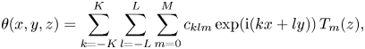 \begin{equation} \theta(x,y, z) = \sum_{k ={-}K}^K \sum_{l ={-}L}^L \sum_{m=0}^{M} c_{klm} \exp({\mathrm{i} (k x + l y)})\,T_m(z), \end{equation}
i.e. a basis of Fourier modes in the horizontal, and Chebyshev polynomials in the vertical (Burns et al. Reference Burns, Vasil, Oishi, Lecoanet and Brown2020). However, the same group theory ideas can be exploited whatever choice of basis is made. Since  $\theta$ (the temperature perturbation) is a real variable, $c^*_{klm} = c_{\bar {k}\,\bar {l}\,m}$.
Suppose that there is an  $N$-dimensional set of coefficients describing the given state. Each symmetry can be represented by an $N\times N$ matrix that describes the action of that symmetry on the basis coefficients (here, the set of $c_{klm}$). In general, this $N\times N$ representation is reducible, and it is possible to change basis such that in the new basis, the components transform according to the irreducible representations of the given group.
The change of basis is achieved using projection operators. To project onto the components that transform according to the  $J$th irrep of a group $G$, we apply the operator $\boldsymbol{\mathsf{P}}^J$ defined by
 \begin{equation} \boldsymbol{\mathsf{P}}^J = \frac{\operatorname{dim} J}{| G| } \sum_{g \in G} (\chi^J (g))^* \boldsymbol{\mathsf{g}}, \end{equation}
where  $\operatorname {dim} J$ is the dimension of the irrep, $| G|$ is the order of the group, $\chi ^J(g)$ is the character of the element $g$, and $\boldsymbol{\mathsf{g}}$ is the matrix representing the action of the element $g$ in the given representation. Moreover, it should be noted that through a change of basis, the representations can be made unitary (orthogonal in the case of real representations) using Weyl's unitary trick. In turn, an orthogonal projection matrix can be used to give an orthogonal set of basis vectors corresponding to a particular irrep using a QR decomposition.
An illustration of an isotypic decomposition into basis vectors that transform according to the irreps is given in figure 5. This example considers the  $c_{210}$ coefficient, and the coefficients to which it can be related using the layer symmetry $p4/nmm$. The periodicity of the computational domain is assumed to align with the principal lattice of translations of $p4/nmm$. As such, the basis vectors $c_{klm}$ are invariant under the group $T$ of lattice translations, so one need only consider the factor group $G/T$ whose character table is given in table 2. There are 8 coefficients that are related by symmetry to $c_{210}$, and the 8 dimensional space can be decomposed into the irreps given in table 2 as the direct sum $A_{1g} \oplus A_{2g} \oplus B_{1g} \oplus B_{2g} \oplus 2 E_u$ (see Dionne et al. (Reference Dionne, Silber and Skeldon1997) for an application of this particular decomposition).
An example of an isotypic decomposition for the wavevector star generated by  $\boldsymbol {k} = (2, 1)$ with no $z$-dependence, i.e. the decomposition into the irreps of $p4/nmm$ given in table 2. The star decomposes as $A_{1g} \oplus A_{2g} \oplus B_{1g} \oplus B_{2g} \oplus 2 E_u$.
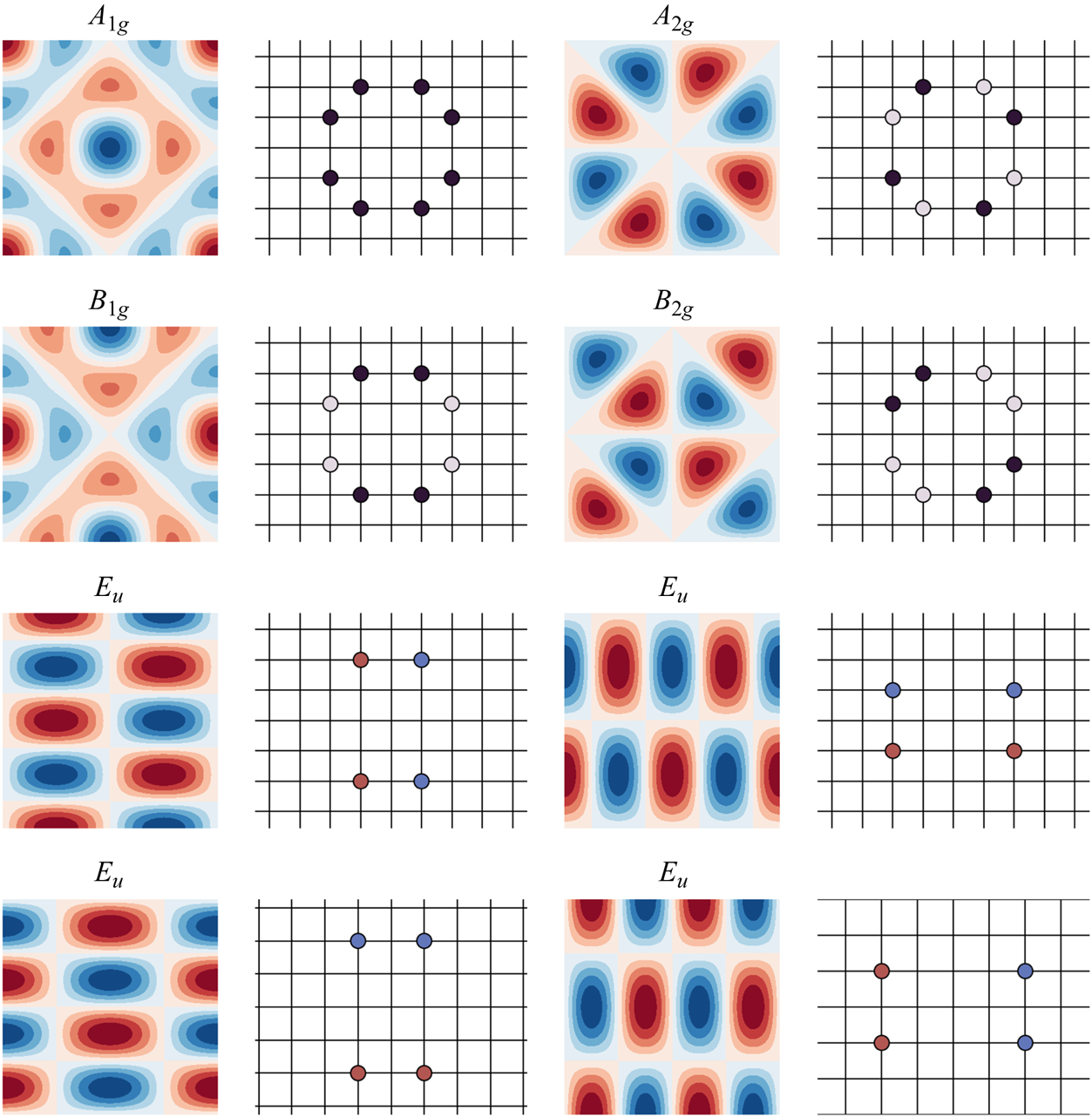
The isotypic decomposition can be used to simplify the numerical study of symmetry-breaking bifurcations. An example of this is shown in figures 6, 7 and 8, which illustrate the breaking of a  $p4/nmm$ pattern of squares into two different planforms with less symmetry, one of $pmmn$ and one of $p4mm$. The computational domain is a box, with aspect ratio such that the distance between rising and sinking regions is 8 times the layer depth. The heat flux is fixed on the top and bottom boundaries, and both boundaries are free-slip. Fixed-flux convection with free-slip boundaries in an infinite layer formally has $k=0$ as the most unstable wavenumber, with critical Rayleigh number ${\textit {Ra}}_c = 120$ (Chapman & Proctor Reference Chapman and Proctor1980; Rieutord Reference Rieutord2015). For the finite horizontal scale of the numerical problem, the critical Rayleigh number is slightly higher, ${\textit {Ra}}_c = 126$. Figure 6(a) shows the planform near onset, at ${\textit {Ra}}=200$, which is dominated by the four modes on the critical circle $|\boldsymbol {k}| = k_c$ although there are also small contributions from higher modes.
Examples of symmetry-breaking bifurcations in fixed-flux convection in a fluid layer, as images of the mid-plane temperature field, both in real space (contour plots) and in reciprocal space (dot patterns). At the onset of convection, a square planform is seen, with  $p4/nmm$ symmetry (layer group 64). The left-hand plots show the evolution of the $p4/nmm$ solution as the Rayleigh number is increased from (a) ${\textit {Ra}} = 200$, (b) ${\textit {Ra}} = 700$, and (c) ${\textit {Ra}} = 1500$. The $p4/nmm$ solution at ${\textit {Ra}} = 1500$ is unstable to perturbations that break the symmetry. (d,e) New solutions at ${\textit {Ra}} = 1500$ that emerge from pitchfork bifurcations from the $p4/nmm$ solution: (d) has symmetry $pmmn$ (layer group 46), and (e) has symmetry $p4mm$ (layer group 55).
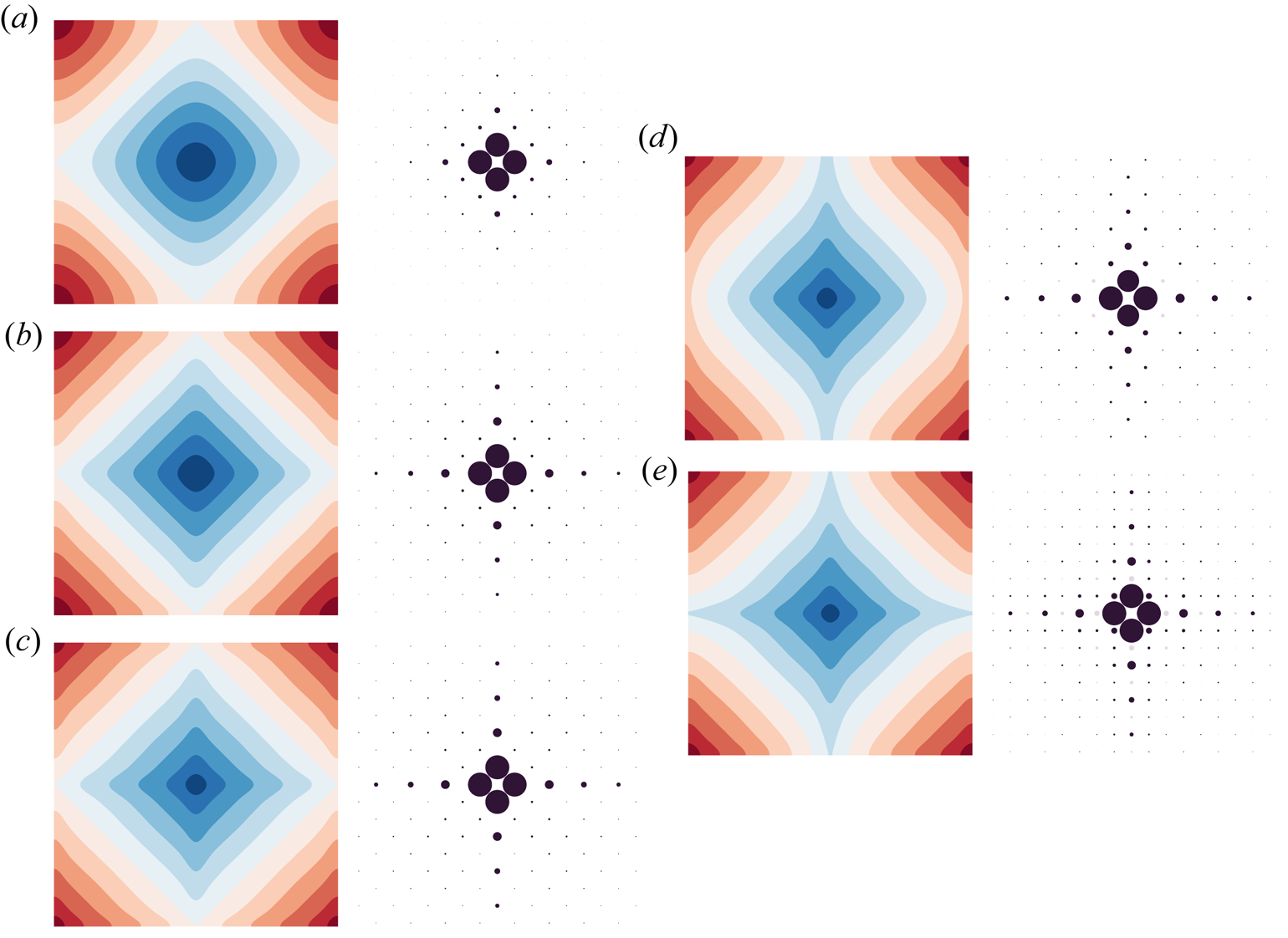
Three-dimensional rendering of the convective flows shown in horizontal cross-section in figures 6(c–e), showing equally-spaced contours of the temperature field. All flows have  ${\textit {Ra}} = 1500$, with symmetries (a) $p4/nmm$, (b) $pmmn$, (c) $p4mm$. The loss of the fourfold vertical rotation symmetry $4_z$ about the centre of the box in going from (a) to (b) can be seen clearly. The loss of symmetry between (a) and (c) is more subtle: the upwellings are now not related by symmetry to the downwellings. Image (c) has lost the horizontal glide reflection $n$, the twofold rotations about horizontal axes, and the twofold screw rotations about horizontal axes (see figure 2).
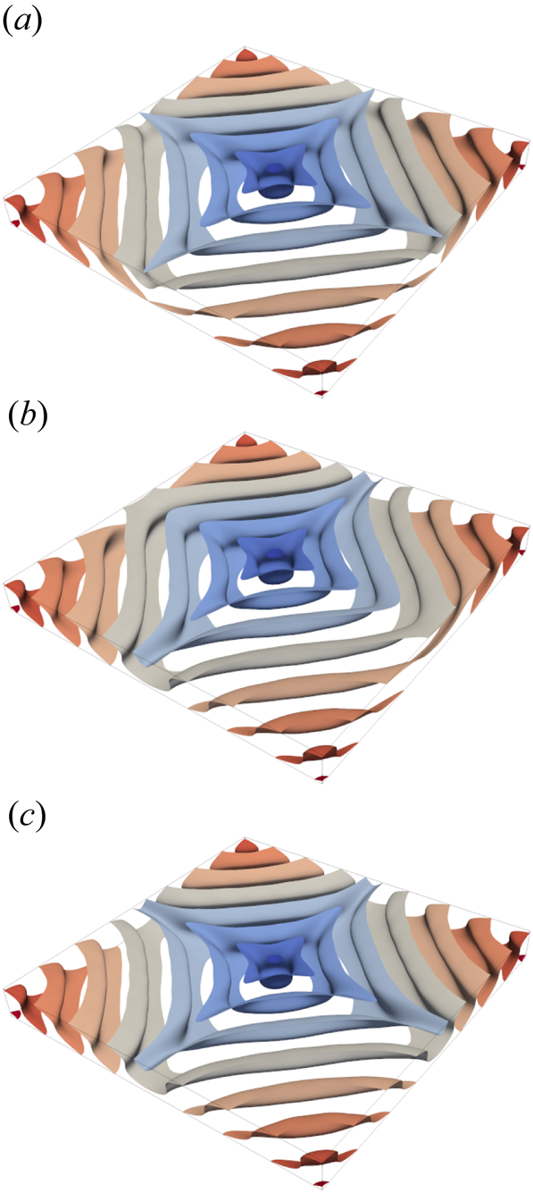
Plots identical to those in figures 6(c–e) but with the origin of the coordinate system shifted by  $(\tfrac {1}{4}, \tfrac {1}{4}, 0)$ (the coordinate system given as origin choice 2 for $p4/nmm$ in ITE). The corresponding symmetry diagrams (with origin shifted from figure 2) are shown on the left. All flows have ${\textit {Ra}} = 1500$, with symmetries (a) $p4/nmm$, (b) $pmmn$, (c) $p4mm$. Some of the symmetry losses are clearer to see with this choice of origin as the rotation axes are moved away from the edges of the box. The loss of the fourfold inversion axes ( $\bar {4}_z$) in going from (a) to (b) or (c) can be seen clearly. The temperature perturbation is necessarily zero on the mid-plane at a fourfold inversion axis.
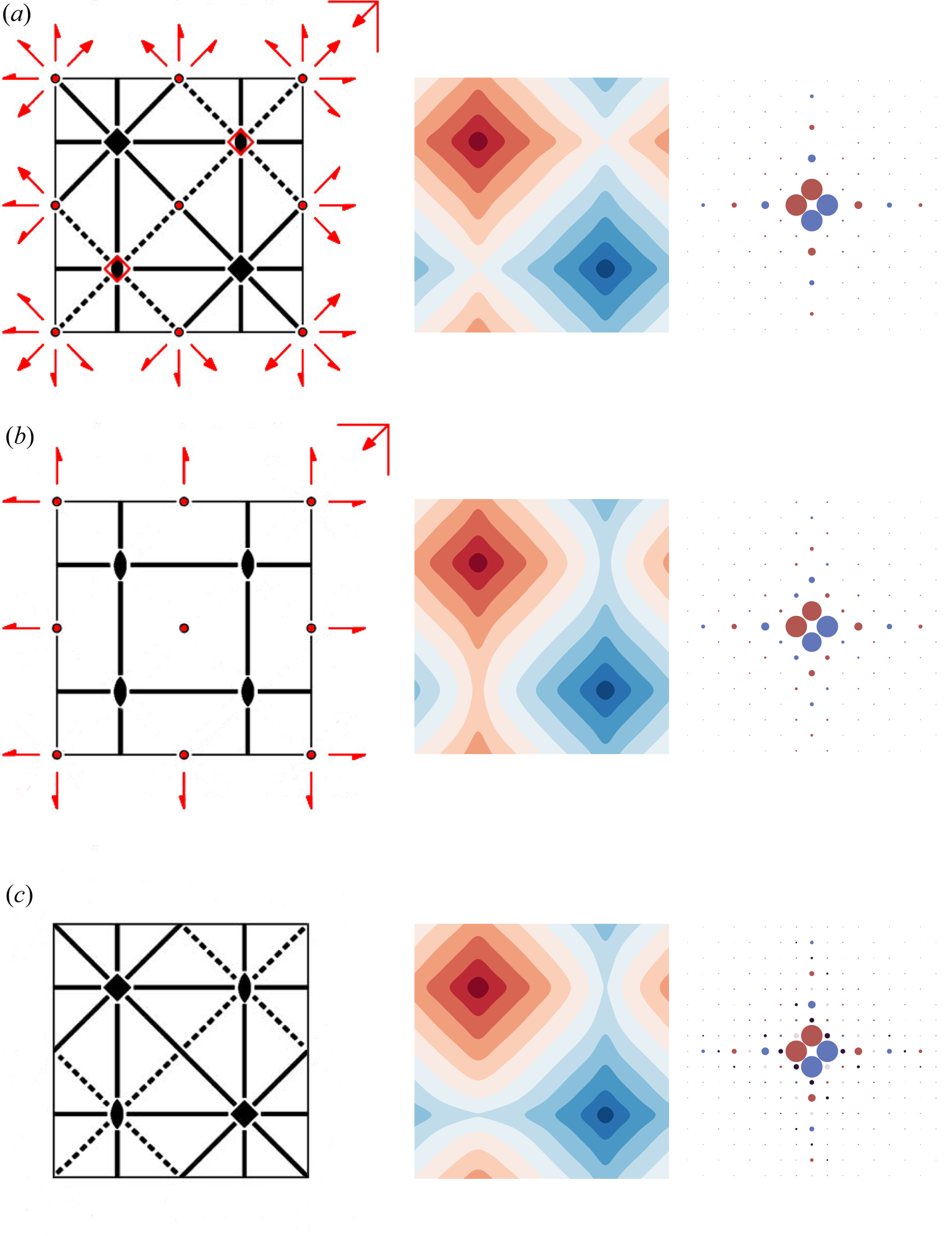
As the Rayleigh number is increased, there is more power in higher modes (figures 6b,c) and sharper features are seen. However, the solution shown in figure 6(c) (and also figures 7(a) and 8(a)) at  ${\textit {Ra}}=1500$ is actually unstable to perturbations that break the symmetry. The unstable solution can be computed by imposing the $p4/nmm$ symmetry on the numerical scheme, either by restricting the set of basis vectors used to those associated with the trivial irrep $A_{1g}$, or by projecting the solutions onto that irrep at each iteration using the projection operator. Restricting the set of basis vectors used is more advantageous in terms of computational efficiency, as one then solves a problem with a much smaller set of unknowns.
Figures 6, 7 and 8 illustrate the same symmetry-breaking transitions, but do so using different projections of the numerical solutions. Figures 6(c), 7(a) and 8(a) show the unstable  $p4/nmm$ solution; figures 6(d), 7(b) and 8(b) show the symmetry break to a $pmmn$ solution; figures 6(e), 7(c) and 8(c) show the symmetry break to a $p4mm$ solution. Both figures 6 and 8 show the mid-plane plane temperature field and its corresponding reciprocal space plot; the only difference is the choice of origin. Figure 6 uses what is given in ITE as origin choice 1 for $p4/nmm$, the same as used in the symmetry diagrams of figure 2. Figure 8 uses an origin that is shifted by $(\tfrac 14, \tfrac 14, 0)$ and referred to as origin choice 2 in ITE. Figure 7 give a three-dimensional rendering of the isotherms in origin choice 1 coordinates.
The loss of symmetry is perhaps clearest to see in the origin choice 2 mid-plane images of figure 8. The loss of the fourfold rotation axes in going from figure 8(a) ( $p4/nmm$) to figure 8(b) ( $pmmn$) is particularly apparent. The loss of symmetry in going from figure 8(a) ( $p4/nmm$) to figure 8(c) ( $p4mm$) is more subtle, as it involves the loss of the glide reflection about the horizontal mid-plane. The upwellings in figure 8(c) are no longer related by symmetry to the downwellings as they are in figure 8(a). This change can be seen in the differences between the shapes of the blue contours (cold downwellings) and the red contours (hot upwellings) in figure 8(c): there are narrow connections between the blue downwelling regions, but no connections between the red upwelling regions. These connections can also be seen in the three-dimensional rendering of figure 7(c), coming through the middle of each side of the box as light blue contours.
The stability of the  $p4/nmm$ solution as a function of Rayleigh number can be assessed using standard linear stability analysis, but the calculations can be made more efficient by exploiting the symmetry. A good general introduction to the numerical methods for performing linear stability and bifurcation analysis can be found in Tuckerman & Barkley (Reference Tuckerman and Barkley2000). The stability analysis relies on the calculation of the eigenvalues of an appropriate Jacobian matrix. When an eigenvalue has a real part that goes from being negative to being positive, there is instability and an associated bifurcation to a new flow pattern. The isotypic decomposition aids the linear stability analysis by allowing one to block-diagonalise the Jacobian according to the irreps. This has several advantages: (i) there are smaller linear systems to deal with in the individual blocks; (ii) the eigenvalues in the individual blocks may be more widely separated that those of the full problem, speeding up convergence of numerical eigenvalue techniques; (iii) one can directly identify the symmetries that are broken and the corresponding active irrep.
Figure 9 illustrates the linear stability analysis of the  $p4/nmm$ solution in figure 6(b) at ${\textit {Ra}}=700$, showing the eigenmodes with largest real part corresponding to the irreps $B_{1g}$ and $A_{2u}$. At ${\textit {Ra}}=700$, eigenvalues of both modes are real and negative. However, for slightly larger ${\textit {Ra}}$, at ${\textit {Ra}}=756$ for $B_{1g}$ and ${\textit {Ra}}=815$ for $A_{2u}$, the eigenvalues become positive, leading to bifurcations and the solutions with broken symmetry seen in figures 6(d,e) (and also figures 7(b,c) and 8(b,c)). Given the irreps involved, these bifurcations are necessarily pitchfork bifurcations.
Examples of eigenmodes in a linear stability analysis of the  $p4/nmm$ solution depicted in figure 6(b), with ${\textit {Ra}}=700$ (using origin choice 1). (a) The mid-plane temperature field for the eigenmode with eigenvalue with largest real part that transforms according to the irrep $B_{1g}$ in table 2, associated with the bifurcation to the $pmmn$ solution in figure 6(d). (b) The corresponding eigenmode that transforms according to irrep $A_{2u}$ in table 2, associated with bifurcation to $p4mm$ in figure 6(e).
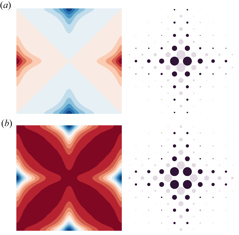
Symmetry can also be exploited to calculate the new equilibrium states after a bifurcation. The solution without the symmetry break can be used as an initial condition, with a small perturbation added in the form of the symmetry-breaking eigenmode of the linear stability calculation. One can use the projection operators to constrain the solution to have the appropriate symmetry (e.g. for figure 6(d), imposing the group  $pmmn$ or restricting to only those basis vectors corresponding to the irreps $A_{1g}$ and $B_{1g}$ of $p4/nmm$ in table 2). Once the eigenmodes associated with the bifurcations have been calculated, it is possible to systematically perform a centre manifold reduction to determine the amplitude equations (Carini, Auteri & Giannetti Reference Carini, Auteri and Giannetti2015), although we have not done this here.
7.2. Further examples
There are many examples of flow transitions in fluid layers in the literature, but almost none use the crystallographic notation that has been adopted here. One study that does is McKenzie (Reference McKenzie1988), which describes a wide variety of transitions in convection, particularly those in the experimental studies of a temperature-dependent viscosity fluid by White (Reference White1988). A convective system with a temperature-dependent viscosity is not invariant under reflection in a horizontal mirror plane. As such, the layer groups involved are those without such mirror planes, which are equivalent to those of the 17 plane or wallpaper groups. Many of the examples discussed by McKenzie (Reference McKenzie1988) are pitchfork bifurcations, although it should be noted that the bifurcations that he discusses with factor group  $D_3$ are generically transcritical, and not pitchforks.
8. Conclusions
Our aim in this work has been to demonstrate the utility of the extensive databases in crystallography for understanding transitions in fluid layers. For simplicity, we have focused on steady states, doubly periodic in space, that are described by the crystallographic layer groups. We have not discussed transitions that break the time-translation symmetry (Hopf bifurcations), which involve spatio-temporal group elements that combine space group elements with time translations. The bifurcation theory for such cases is well understood, but it would be helpful to have a standardised crystallographic notation for describing such transitions. Translations in time can be associated with a fourth dimension. Hopf bifurcations lead to solutions that are time-periodic, thus the natural groups to consider will be the subperiodic groups in four dimensions with a three-dimensional lattice of translations (the two horizontal space dimensions and one time dimension). We have also made no attempt here to describe the representation theory for the initial onset of convection; formally, this would involve a study of the representations of  $E(2) \times C_2$, which is a non-compact Lie group. The difficulty of dealing with such a group is usually side-stepped in the literature by considering instead a problem on a compact domain (the two-torus). The analysis of pattern-forming problems is considerably more straightforward when they are forced to be periodic with respect to a lattice, as they have been in this paper. The spectrum of modes is discrete, and techniques like centre manifold reduction can be used. Patterns that are not exactly periodic are more challenging to analyse, but there are techniques available (see, for example, Chapters 7–11 of Hoyle Reference Hoyle2006). Such methods are required for understanding phenomena such as defects, dislocations, the zig-zag and cross-roll instabilities, spirals and quasi-patterns.
There is a wealth of useful information that lies within the crystallographic databases, and we encourage fluid dynamicists to exploit it.
Supplementary materials
Three supplements with additional group theory tables are available at https://doi.org/10.1017/jfm.2024.482.
Acknowledgements
We thank J. Dawes, A. Rucklidge and three anonymous reviewers for their helpful comments on this work. We also thank N. Balmforth for his editorial handling.
Funding
This research received no specific grant from any funding agency, commercial or not-for-profit sectors.
Declaration of interests
The authors report no conflict of interest.
Appendix A. The symmetries of Rayleigh–Bénard convection
Consider Rayleigh–Bénard convection in a fluid layer, with  $x$ and $y$ as horizontal coordinates, and $z$ as a vertical coordinate. The system has a natural Euclidean symmetry in the horizontal plane, represented by the group $E(2)$. However, depending on boundary conditions and rheological choices, there may be additional symmetries in the problem.
A.1. Governing equations
For Boussinesq, infinite Prandtl number, thermal convection the governing equations are
 \begin{gather} \boldsymbol{\nabla}\boldsymbol{\cdot} \boldsymbol{v} = 0, \end{gather}
 \begin{gather}\boldsymbol{\nabla}\boldsymbol{\cdot} {\sigma} ={-} \rho_0 g \alpha T \hat{\boldsymbol{z}}, \end{gather}
 \begin{gather}\frac{\partial T}{\partial t} + \boldsymbol{v} \boldsymbol{\cdot} \boldsymbol{\nabla} T = \kappa\,\nabla^2T, \end{gather}
where  $\boldsymbol {v}$ is the fluid velocity, ${\sigma }$ is the stress tensor, $\rho _0$ is the reference density, $g$ is the acceleration due to gravity, $\alpha$ is the thermal expansivity, $T$ is the temperature, and $\kappa$ is the thermal diffusivity. The Newtonian constitutive law relating stress to strain rate is
 \begin{equation} {\sigma} ={-} p {\mathsf{I}} + \eta \left(\boldsymbol{\nabla} \boldsymbol{v} + \boldsymbol{\nabla} \boldsymbol{v}^\mathrm{T} \right), \end{equation}
where  $p$ is the pressure. Let $\theta$ represent the temperature perturbation from a conductive steady state, where the steady-state temperature gradient is $\Delta T / a$, and $a$ is the layer thickness. The governing equations (A1), (A2) and (A3) can be rewritten as
 \begin{gather} \boldsymbol{\nabla} \boldsymbol{\cdot} \boldsymbol{v} = 0, \end{gather}
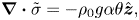 \begin{gather}\boldsymbol{\nabla}\boldsymbol{\cdot} \tilde{{\sigma}} ={-} \rho_0 g \alpha \theta \hat{\boldsymbol{z}}, \end{gather}
 \begin{gather}\frac{\partial \theta}{\partial t} + \boldsymbol{v} \boldsymbol{\cdot}\boldsymbol{\nabla} \theta - \frac{\Delta T}{a}\,\boldsymbol{v} \boldsymbol{\cdot} \hat{\boldsymbol{z}} = \kappa\,\nabla^2 \theta, \end{gather}
where  $\tilde {{\sigma }}$ is a modified stress tensor that represents the difference from the conductive state. The equations can be made dimensionless by scaling all lengths by the layer thickness $a$, and all times by the diffusion time $a^2/\kappa$. The behaviour is controlled by the dimensionless Rayleigh number ${\textit {Ra}} = \rho _0 g \alpha \,\Delta T\,a^3 / (\eta _0 \kappa )$. The temperature can be scaled by $\Delta T / {\textit {Ra}}$, the velocity by $\kappa /a$, and the pressure by $\rho _0 g \alpha \theta _0 d$, to yield
 \begin{gather} \boldsymbol{\nabla}\boldsymbol{\cdot} \boldsymbol{v} = 0, \end{gather}
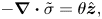 \begin{gather}- \boldsymbol{\nabla}\boldsymbol{\cdot}\tilde{{\sigma}} = \theta \hat{\boldsymbol{z}}, \end{gather}
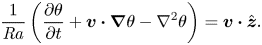 \begin{gather}\frac{1}{{\textit{Ra}}} \left( \frac{\partial \theta}{\partial t} + \boldsymbol{v} \boldsymbol{\cdot}\boldsymbol{\nabla}\theta - \nabla^2 \theta \right) = \boldsymbol{v} \boldsymbol{\cdot} \hat{\boldsymbol{z}}. \end{gather}
A.2. Mid-plane reflection
If boundary conditions top and bottom are identical, then provided that the viscosity is constant (or depth-dependent with mid-plane symmetry), the equations are invariant under the mid-plane symmetry (where  $z=0$ is the mid-plane)
 \begin{equation} m_z: (x, y, z) \rightarrow (x, y, -z), \end{equation}
provided that the variables in the equations transform as
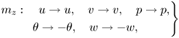 \begin{equation} \left.\begin{gathered} m_z: \quad u \rightarrow u, \quad v \rightarrow v, \quad p \rightarrow p, \\ \theta \rightarrow - \theta, \quad w \rightarrow - w, \end{gathered}\right\}\end{equation}
where the velocity vector is  $\boldsymbol {v} = (u, v, w)$, and $p$ is the pressure perturbation. Here, (A12) represents the symmetry between hot upwellings and cold downwellings.
A.3. Poloidal-toroidal decomposition
For three-dimensional flows represented by poloidal and toroidal potentials  $\mathcal {S}$ and $\mathcal {T}$ (and neglecting any mean-field flow), we have
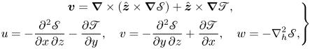 \begin{equation} \left.\begin{gathered} \boldsymbol{v} = \boldsymbol{\nabla} \times (\hat{\boldsymbol{z}} \times \boldsymbol{\nabla} \mathcal{S}) + \hat{\boldsymbol{z}} \times \boldsymbol{\nabla} \mathcal{T}, \\ u ={-} \frac{\partial^2 \mathcal{S}}{\partial x\,\partial z} - \frac{\partial \mathcal{T}}{\partial y}, \quad v ={-} \frac{\partial^2 \mathcal{S}}{\partial y\,\partial z} + \frac{\partial \mathcal{T}}{\partial x}, \quad w ={-} \nabla^2_h \mathcal{S}, \end{gathered}\right\} \end{equation}
so the potentials must transform under mid-plane reflection as
 \begin{equation} m_z: \quad \mathcal{S} \rightarrow - \mathcal{S}, \quad \mathcal{T} \rightarrow \mathcal{T}. \end{equation}
This is different from their transformation under vertical mirrors, which is
 \begin{equation} m_x: \quad \mathcal{S} \rightarrow \mathcal{S}, \quad \mathcal{T} \rightarrow - \mathcal{T} \end{equation}
as  $m_x: u \rightarrow - u$. For the constant-viscosity example in figure 6, the flow is purely poloidal ( $\mathcal {T}=0$). The poloidal potential $\mathcal {S}$ transforms in the same way as the temperature perturbation $\theta$ under the symmetry operations.
While this work uses the Cartesian coordinates of the plane layer, it should be noted that poloidal–toroidal decompositions are commonly used in problems of spherical geometry, such as the study of convection in a spherical shell in mantle dynamics (Ribe Reference Ribe2018). Indeed, symmetry arguments can be similarly exploited in a spherical geometry to understand the nature of the bifurcations (Chossat, Lauterbach & Melbourne Reference Chossat, Lauterbach and Melbourne1991; Matthews Reference Matthews2003).
A.4. Time dimension
This work focuses on steady states, thus there is little discussion of the time dimension. However, it is worth noting that while the governing equations are invariant under any time translation, they are not invariant under time reflection  $m_t$ owing to the diffusion term.
A.5. Self-adjointness
If (A1), (A2) and (A3) are linearised about a conductive steady state (i.e. neglecting the  $\boldsymbol {v} \boldsymbol {\cdot }\boldsymbol {\nabla } \theta$ term), then the equations themselves have an important symmetry: namely, they are self-adjoint provided that the viscosity is constant or purely depth dependent, and appropriate boundary conditions are applied.
Appendix B. Representations of layer groups with non-zero wavevector
The general theory of representations of layer groups with a non-zero wavevector is somewhat involved, and a full account can be found in e.g. Bradley & Cracknell (Reference Bradley and Cracknell1972), Aroyo et al. (Reference Aroyo, Kirov, Capillas, Perez-Mato and Wondratschek2006a), de la Flor et al. (Reference de la Flor, Souvignier, Madariaga and Aroyo2021) and Grenier & Ballou (Reference Grenier and Ballou2012). In this appendix, we give some simple examples of representations with a non-zero wavenumber that are associated with spatial-period-multiplying bifurcations.
Consider the layer group  $p4mm$ (no. 55). This group can be generated by unit translations $t_x$ and $t_y$ in the $x$- and $y$-directions, along with point group element $4_z$ representing a $90^\circ$ rotation about the $z$-axis, and point group element $m_{\bar {x}y}$ representing a reflection in a vertical mirror plane parallel to the line $y=x$. A representation of the group can be described by a mapping of the generators to a set of matrices.
In the general theory of representations of layer groups, each irreducible representation is described by a wavevector  $\boldsymbol {k}$ and a label for a particular small representation of the wavevector. For this example, we consider a wavevector of the form
 \begin{equation} \boldsymbol{k} = u \boldsymbol{a}_1^* + u \boldsymbol{a}_2^*, \end{equation}
where  $u<1/2$, and $\boldsymbol {a}_1^*, \boldsymbol {a}_2^*$ are basis vectors for the reciprocal lattice, defined such that $\boldsymbol {a}_i \boldsymbol {\cdot }\boldsymbol {a}_j^* = 2 {\rm \pi}\delta _{ij}$, where $\boldsymbol {a}_1$ and $\boldsymbol {a}_2$ are the space domain basis lattice vectors. The wavevector lies in a subset of the Brillouin zone known as the representation domain (figure 10).
The Brillouin zone for  $p4/nmm$ from the BCS (de la Flor et al. Reference de la Flor, Souvignier, Madariaga and Aroyo2021). The irreps are specified by a wavevector lying in the labelled triangular region, known as the representation domain. The origin is at the $\varGamma$ point. The special point $M$ is at $(\tfrac {1}{2}, \tfrac {1}{2})$. Software that uses text labels will refer to $\varGamma$ as GM, $\varDelta$ as DT, and $\varSigma$ as SM.
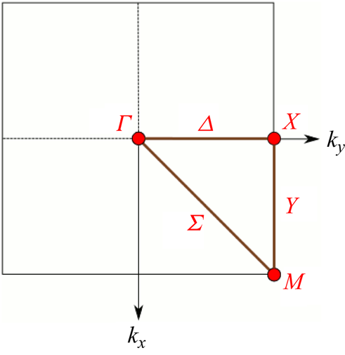
The chosen wavevector in (B1) lies within the part of the Brillouin zone labelled  $\varSigma$ (written as SM in software that uses text labels). The tool LKVEC (de la Flor et al. Reference de la Flor, Souvignier, Madariaga and Aroyo2021) on the BCS can be used to identify the position of a wavenumber vector in the representation domain and the corresponding little co-group $\bar {G}^{\boldsymbol {k}}$. The little co-group is the set of point group elements that leaves the wavevector unchanged. The little co-group associated with wavevectors along $\varSigma$ is $..m$, which has just two elements: the identity and the mirror $m_{\bar {x}y}$.
From the little co-group  $\bar {G}^{\boldsymbol {k}}$, one can form the little group $G^{\boldsymbol {k}}$ of $\boldsymbol {k}$, which is a subgroup of $G$ containing those elements that have the point group elements of the little co-group in their rotational part. We first need to obtain representations of the little group. Such representations must be small (or allowed) representations, which are the representations of the little group that map a pure translation by a vector $\boldsymbol {d}$ to $\exp (- \textrm {i} \boldsymbol {k} \boldsymbol {\cdot }\boldsymbol {d})$ times an identity matrix. In this simple example, the small representations are one-dimensional, and there are just two of them. The small group is generated by the unit translations and the mirror element $m_{\bar {x}y}$. Since the representations of the translations have been prescribed, all that remains is to describe the mapping of the mirror element. There is a trivial representation $\varSigma _1$ that maps the mirror element $m_{\bar {x}y}$ to 1, and another representation $\varSigma _2$ that maps the mirror element to $-1$.
$-1$.
The star of the wavevector is the set of possible wavevectors that can be obtained by applying all the point group operations to the given wavevector. In this example, the star has four arms:
 \begin{gather} \boldsymbol{k}_1 = (u, u), \end{gather}
 \begin{gather}\boldsymbol{k}_2 = ({-}u, -u), \end{gather}
 \begin{gather}\boldsymbol{k}_3 = (u, -u), \end{gather}
 \begin{gather}\boldsymbol{k}_4 = ({-}u, u). \end{gather}
The left cosets of  $G^{\boldsymbol {k}}$ in $G$ are in one-to-one correspondence with the star of the wavevector. A representation of the full group $G$ can be obtained as an induced representation from the little group $G^{\boldsymbol {k}}$. The induced representation is of dimension $m d$, where $d$ is the dimension of the little group representation (here $d=1$), and $m$ is the number of left cosets of $G^{\boldsymbol {k}}$ in $G$ (which is identical to the number of arms in the star of the wavevector, here $m=4$).
In the induced representation, a general translation by a vector  $\boldsymbol {d} = (d_1, d_2)$ is represented by a diagonal matrix of the form
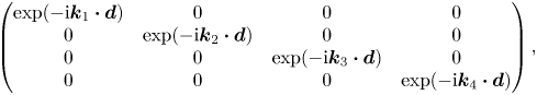 \begin{equation} \begin{pmatrix} \exp({-\mathrm{i} \boldsymbol{k}_1 \boldsymbol{\cdot} \boldsymbol{d}}) & 0 & 0 & 0\\ 0 & \exp({-\mathrm{i} \boldsymbol{k}_2 \boldsymbol{\cdot} \boldsymbol{d}}) & 0 & 0 \\ 0 & 0 & \exp({-\mathrm{i} \boldsymbol{k}_3 \boldsymbol{\cdot} \boldsymbol{d}}) & 0 \\ 0 & 0 & 0 & \exp({-\mathrm{i} \boldsymbol{k}_4 \boldsymbol{\cdot} \boldsymbol{d}}) \\ \end{pmatrix}, \end{equation}
where  $\boldsymbol {k}_1$, $\boldsymbol {k}_2$, $\boldsymbol {k}_3$ and $\boldsymbol {k}_4$ are the arms of the star.
The induced representation  $^*\varGamma _1$ of the full space group $G$ is given in terms of the generators as
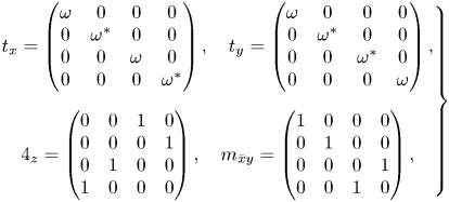 \begin{equation} \left.\begin{gathered} t_x = \begin{pmatrix} \omega & 0 & 0 & 0 \\ 0 & \omega^* & 0 & 0 \\ 0 & 0 & \omega & 0 \\ 0 & 0 & 0 & \omega^* \\ \end{pmatrix}, \quad t_y = \begin{pmatrix} \omega & 0 & 0 & 0 \\ 0 & \omega^* & 0 & 0 \\ 0 & 0 & \omega^* & 0 \\ 0 & 0 & 0 & \omega \\ \end{pmatrix}, \\ 4_z = \begin{pmatrix} 0 & 0 & 1 & 0 \\ 0 & 0 & 0 & 1 \\ 0 & 1 & 0 & 0 \\ 1 & 0 & 0 & 0 \\ \end{pmatrix}, \quad m_{\bar{x}y} = \begin{pmatrix} 1 & 0 & 0 & 0 \\ 0 & 1 & 0 & 0 \\ 0 & 0 & 0 & 1 \\ 0 & 0 & 1 & 0 \\ \end{pmatrix}, \end{gathered}\right\} \end{equation}
where  $\omega = \exp ({-2 {\rm \pi}\mathrm {i} u})$. The representation $^*\varGamma _2$ has identical generators, except for $m_{\bar {x}y}$, which has $-1$ in place of $1$ in each entry. The above representation has complex entries, but by a change of basis, an equivalent real representation can be found.
If the wavevector of form (B1) is chosen with  $u=1/2$, then it lies at a special point in the Brillouin zone labelled $M$. The little co-group is then $4mm$, and the induced representation $^*M_1$ from the trivial representation of the little group is simply the one-dimensional representation that maps the generators as
 \begin{equation} t_x ={-}1, \quad t_y ={-}1, \quad 4_z = 1, \quad m_{\bar{x}y} = 1. \end{equation}
There are four additional representations induced from the little group, including a two-dimensional representation  $^*M_5$, but these will not be considered further.
B.1. Application to spatial-period-multiplying bifurcations
The representations  $^*\varGamma _1$ and $^*M_1$ with matrices given in (B7) and (B8a–d) can be used to describe spatial-period-multiplying bifurcations for $p4mm$. The simplest case is when $u = 1/2$, and the one-dimensional representation $^*M_1$ in (B8a–d) provides a mapping onto the group $C_2$. There is an isotropy subgroup that consists of all those elements that map to 1. This subgroup is also $p4mm$ (as all the point group elements are retained), but it has a reduced set of translation elements (it is an index-2 klassengleiche subgroup). For the subgroup, a new basis for the lattice can be obtained using the translations by $(1, 1)$ and $(1, -1)$. This isotropy subgroup is the maximal isotypic subgroup of lowest index for $p4mm$.
For the representation  $^*\varGamma _1$, suppose that $u=1/p$, where $p$ is a prime number equal to 3 or greater. Then $\omega ^p = 1$, and the matrix group described by (B7) is the finite group $D_4 \ltimes C_p^2$ of order $8 p^2$. There is a klassengleiche axial isotropy subgroup of this representation of $p4mm$ that is also $p4mm$ but with the basis vectors of the lattice scaled by factor $p$ in each direction (the index of the subgroup in the parent group is $p^2$). All the point group operations are retained in the subgroup. In the representation in (B7), this can be recognised explicitly by the fixed-point subspace $(a, a, a, a)$, which is invariant under $4_z$ and $m_{\bar {x}y}$ (retaining the point group) and the translations for which $(d_1, d_2) \equiv (0, 0) \, (\operatorname {mod} p)$. There are also non-isotypic axial isotropy subgroups of $^*\varGamma _1$ with fixed-point subspaces $(b, b, 0, 0)$ and $(0, 0, c, c)$. For these isotropy subgroups, the point group is reduced to $mm2$, consisting of the diagonal mirrors and $2_z$. The translation group is reduced, but retains the diagonal translation with multiples of either $(1, -1)$ or $(1, 1)$. The corresponding layer group is $cmm2$ (index- $2p$ subgroup).
For the particular case  $p=3$, the character table for the group $D_4 \ltimes C_3^2$ is given in supplement 3, and further discussion of its role in spatial-period-multiplying bifurcations can be found in Matthews (Reference Matthews2004) (see his figure 1).
B.2. An example of $p4/nmm$

A slightly more complicated, but closely related, example is given by  $p4/nmm$ (no. 64). This is a non-symmorphic layer group. It can be generated by the same operations as $p4mm$, i.e. $t_x$, $t_y$, $4_z$ and $m_{\bar {x}y}$, but in addition is generated by a glide reflection $n$ that reflects in a vertical mirror $m_z$ and then translates by $(\tfrac {1}{2}, \tfrac {1}{2}, 0)$. An index-9 $k$-transition from $p4/nmm$ to $p4/nmm$ can be obtained as an isotropy subgroup of two different irreps: the irrep $^* \varSigma _1$ with wavevector $\boldsymbol {k} = (\tfrac 13, \tfrac 13)$ given by
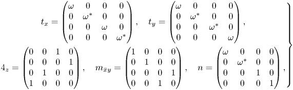 \begin{equation} \left.\begin{gathered} t_x = \begin{pmatrix} \omega & 0 & 0 & 0 \\ 0 & \omega^* & 0 & 0 \\ 0 & 0 & \omega & 0 \\ 0 & 0 & 0 & \omega^* \\ \end{pmatrix}, \quad t_y = \begin{pmatrix} \omega & 0 & 0 & 0 \\ 0 & \omega^* & 0 & 0 \\ 0 & 0 & \omega^* & 0 \\ 0 & 0 & 0 & \omega \\ \end{pmatrix}, \\ 4_z = \begin{pmatrix} 0 & 0 & 1 & 0 \\ 0 & 0 & 0 & 1 \\ 0 & 1 & 0 & 0 \\ 1 & 0 & 0 & 0 \\ \end{pmatrix}, \quad m_{\bar{x}y} = \begin{pmatrix} 1 & 0 & 0 & 0 \\ 0 & 1 & 0 & 0 \\ 0 & 0 & 0 & 1 \\ 0 & 0 & 1 & 0 \\ \end{pmatrix}, \quad n = \begin{pmatrix} \omega & 0 & 0 & 0 \\ 0 & \omega^* & 0 & 0 \\ 0 & 0 & 1 & 0 \\ 0 & 0 & 0 & 1 \\ \end{pmatrix}, \end{gathered}\right\}\end{equation}
where  $\omega = \exp ({-2 {\rm \pi}\mathrm {i} /3})$, and the irrep $^* \varDelta _3$ with wavevector $\boldsymbol {k} = (0, \tfrac 13)$ given by
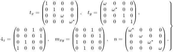 \begin{align} \left.\begin{gathered} t_x = \begin{pmatrix} 1 & 0 & 0 & 0 \\ 0 & 1 & 0 & 0 \\ 0 & 0 & \omega & 0 \\ 0 & 0 & 0 & \omega^* \\ \end{pmatrix}, \quad t_y = \begin{pmatrix} \omega & 0 & 0 & 0 \\ 0 & \omega^* & 0 & 0 \\ 0 & 0 & 1 & 0 \\ 0 & 0 & 0 & 1 \\ \end{pmatrix}, \\ 4_z = \begin{pmatrix} 0 & 0 & 1 & 0 \\ 0 & 0 & 0 & 1 \\ 0 & 1 & 0 & 0 \\ 1 & 0 & 0 & 0 \\ \end{pmatrix}, \quad m_{\bar{x}y} = \begin{pmatrix} 0 & 0 & 1 & 0 \\ 0 & 0 & 0 & 1 \\ 1 & 0 & 0 & 0 \\ 0 & 1 & 0 & 0 \\ \end{pmatrix}, \quad n = \begin{pmatrix} \omega^* & 0 & 0 & 0 \\ 0 & \omega & 0 & 0 \\ 0 & 0 & \omega^* & 0 \\ 0 & 0 & 0 & \omega \\ \end{pmatrix}. \end{gathered}\right\}\end{align}
For both representations (B9) and (B10),  $(a, a, a, a)$ is the fixed-point subspace corresponding to the axial isotropy subgroup $p4/nmm$. Note that for both cases, $t_x^3$, $t_y^3$ and $n^3$ map to the identity and so are elements of the isotropy subgroup. Here, $n^3$ represents a reflection in a vertical mirror followed by a translation by $(\tfrac 32, \tfrac 32, 0)$, so is the same as the original glide reflection $n$ but with the translation vector scaled by 3.
Appendix C. Equivariants and character theory
Much of the key information about symmetry-breaking bifurcations can be obtained from a series of routine mechanical calculations using character tables. As described by Matthews (Reference Matthews2004) and Antoneli et al. (Reference Antoneli, Dias and Matthews2008), these calculations can be automated using the computational algebra package GAP (The GAP Group 2021).
Many key results follow from the trace formula that states that for a group  $G$ acting linearly on a vector space $V$, the dimension of the fixed-point subspace is
 \begin{equation} \text{dim}\,\text{Fix}(G, V) = \langle \chi_V, 1\rangle, \end{equation}
where  $\chi _V$ is the character of the representation of $G$ on $V$, 1 is the trivial character, and angle brackets represent the scalar product on characters. This formula can be used to determine whether a subgroup is an isotropy subgroup (Matthews Reference Matthews2004). Note that $V$ in the trace formula can be any vector space, not just $\mathbb {R}^n$. By applying this formula to appropriately symmetrised parts of tensor product spaces, Antoneli et al. (Reference Antoneli, Dias and Matthews2008) show how it can be used to work out the dimensions of the spaces of invariant and equivariant polynomials (their (3.9) and (3.10)). If $I(k)$ is the dimension of the space of invariant polynomials of degree $k$, and $E(k)$ is the corresponding space of equivariants of degree $k$, then the trace formula yields
 \begin{gather} I(k) = \left\langle \chi_{S^k V}, 1 \right\rangle, \end{gather}
 \begin{gather}E(k) = \left\langle \chi_{S^k V} \chi_{V}, 1 \right\rangle, \end{gather}
where  $S^k V$ refers to the symmetric part of the tensor product of $k$ copies of $V$.
$V$.
As an example, suppose that we want to work out the number of quadratic equivariants for the faithful irrep of  $D_3$. The character of the irrep can be written as $\chi _V = (2, 0, -1)$, where the identity corresponds to 2, the mirrors correspond to 0, and the rotations correspond to $-1$. The symmetric part of $V \otimes V$ has character $\chi _{S^2 V} = (3, 1, 0)$. Thus $\chi _{S^2 V} \chi _V = (6, 0, 0)$. The inner product with the trivial character then yields $E(2) = 6 / 6 = 1$ (since the order of $D_3$ is 6). Supplement 3 provides tables of $I(k)$ and $E(k)$ for a series of small finite groups.


 Open access