


1. Introduction
Volvox is a genus of algae, several species of which form spherical, free-swimming colonies consisting of up to 50 000 somatic cells embedded in an extracellular matrix on the surface, with interior germ cells that develop into a small number of colonies of the next generation. The colony has an anterior–posterior axis of symmetry and each somatic cell bears a pair of beating flagella that enable the colony to swim approximately parallel to this axis. Each cell's flagella beat in approximately the same direction (relative to the colony), i.e. in a plane that is offset from a purely meridional plane by an angle of  $10^\circ \text {--}20^\circ$. This offset causes the colony to rotate about its axis as it swims (Hoops Reference Hoops1993); the rotation is always clockwise when viewed from its anterior pole. In still water colonies tend to swim vertically upwards, on average, because they are bottom heavy (daughter colonies being clustered towards the rear), although they are slightly (approximately 0.3 %) denser than water and therefore sediment downwards when the flagella are inactivated. The beating of the flagella of cells at different polar angles, $\theta$, has been observed, in colonies held stationary on a micro-pipette, to be coordinated in the form of a symplectic metachronal wave, which propagates from anterior to posterior in the same direction as the power stroke of the flagellar beat (Brumley et al. Reference Brumley, Polin, Pedley and Goldstein2012). Modelling suggests that hydrodynamic interactions between the flagella of different cells, coupled with flagellar flexibility, provide the mechanism for the coordination (Niedermayer, Eckhardt & Lenz Reference Niedermayer, Eckhardt and Lenz2008; Brumley et al. Reference Brumley, Polin, Pedley and Goldstein2012, Reference Brumley, Polin, Pedley and Goldstein2015). A detailed survey of the physics and fluid dynamics of green algae such as Volvox has been given by Goldstein (Reference Goldstein2015).
The radius  $a$ of a Volvox colony increases with age (the lifetime of a V. carteri colony is approximately 48 h) although the number and size of cells do not. Drescher et al. (Reference Drescher, Leptos, Tuval, Ishikawa, Pedley and Goldstein2009) measured the free-swimming properties of many colonies of V. carteri of different radii. Results for the mean upswimming speed $W$, sedimentation speed $V_g$, angular velocity $\varOmega$, mean density difference between a colony and the surrounding fluid (inferred from $V_g$) and time scale $\tau$ for reorientation by gravity when the axis is disturbed from the vertical (a balance between viscous and gravitational torques) are shown in figure 1(a–e). Note that, if the colony were neutrally buoyant but otherwise identical, driven by the same flagellar beating, its swimming speed would be $U = W + V_g$. The largest colonies cannot make upwards progress ( $W<V_g$); they naturally sink towards the bottom of the swimming chamber, even when their flagella continue to perform normal upswimming motions. The colony Reynolds number is always less than approximately $0.15$ so that the hydrodynamics is dominated by viscous forces.
Swimming properties of V. carteri as a function of radius: (a) upswimming speed, (b) rotational frequency, (c) sedimentation speed, (d) bottom-heaviness reorientation time, (e) density offset and (f) components of average flagellar force density. (From Drescher et al. (Reference Drescher, Leptos, Tuval, Ishikawa, Pedley and Goldstein2009), figure 3, with permission.)

Drescher et al. (Reference Drescher, Leptos, Tuval, Ishikawa, Pedley and Goldstein2009) also observed the behaviour of V. carteri colonies as they swim up towards a horizontal glass plane above or sink towards a horizontal plane below. In the former case, the flagella on a colony that is close to the upper surface continue beating and applying tangential thrust to the nearby fluid. Since the fluid is prevented from flowing from above, the flagellar beating pulls in fluid horizontally from all round and thrusts it downwards. This was observed by seeding the fluid with  $0.5\ \mathrm {\mu }\textrm {m}$ polystyrene microspheres and the velocity field measured in horizontal and vertical planes using particle image velocimetry (Drescher et al. Reference Drescher, Leptos, Tuval, Ishikawa, Pedley and Goldstein2009).
The simplest model of a swimming colony (Short et al. Reference Short, Solari, Ganguly, Powers, Kessler and Goldstein2006) ascribes the total mean force exerted by the flagella to a uniform tangential shear stress exerted on the spherical surface, with components  $f_\theta$ and $f_\phi$ in the directions of the polar angle $\theta$ and the azimuthal angle $\phi$. Drescher et al. (Reference Drescher, Leptos, Tuval, Ishikawa, Pedley and Goldstein2009) estimated $f_\theta$ and $f_\phi$, as functions of colony radius $a$, from the measured values of $W$,
$W$,  $V_g$ and $\varOmega$ and low-Reynolds-number hydrodynamics (the Stokes law and the equivalent for rotation)
 \begin{equation} f_\theta = 6\mu (W+V_g)/{\rm \pi} a, \quad f_\phi = 8\mu \varOmega/{\rm \pi}, \end{equation}
where  $\mu$ is the fluid viscosity. The estimated values corresponded to a few pN per flagellar pair, as also found by Solari et al. (Reference Solari, Ganguly, Kessler, Michod and Goldstein2006). It can be inferred from these results that there is a critical colony radius, $a_c$, at which a colony far from any boundaries will hover at rest ( $W=-V_g$). For the experiments shown in figure 1, $a_c \approx 300\ \mathrm {\mu }\textrm {m}$.
When two Volvox colonies of approximately the same size, with  $a < a_c$, were introduced into the chamber, and when they were both spinning near the upper surface, they were observed to attract each other and to orbit around each other in a bound state, termed a ‘waltz’, by Drescher et al. (Reference Drescher, Leptos, Tuval, Ishikawa, Pedley and Goldstein2009) (figure 2a and supplementary movie M1 available at https://doi.org/10.1017/jfm.2020.613). When the individual angular velocity $\varOmega$ was approximately $1\ \textrm {rad}\,\textrm {s}^{-1}$, the orbiting frequency $\omega$ was approximately $0.1\ \textrm {rad}\,\textrm {s}^{-1}$. The mutual attraction is consistent with the radial inflow of small particles to a single colony, and the rate of approach of two nearby colonies close to the top wall can be well approximated by treating each colony as a point Stokeslet at the sphere's centre, together with its image system in the plane (Drescher et al. Reference Drescher, Leptos, Tuval, Ishikawa, Pedley and Goldstein2009). These results provided the first quantitative experimental verification of the prediction by Squires (Reference Squires2001) of a wall-mediated attraction between downward-pointing Stokeslets near an upper no-slip surface.
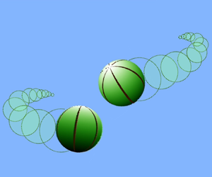
(a) Waltzing of V. carteri: top view. Superimposed images taken 4 s apart, graded in intensity. Scale bar is 1 mm; (b) ‘minuet’ bound state: side views 3 s apart of two colonies near the chamber bottom. Arrows indicate the anterior–posterior axes  ${\boldsymbol {p}}_m$ at angles $\theta _m$ to the vertical. Scale bar is $600\ \mathrm {\mu }\textrm {m}$. (From Drescher et al. (Reference Drescher, Leptos, Tuval, Ishikawa, Pedley and Goldstein2009), figures 1a and 5a, with permission.)

However, the orbiting is not a direct consequence of colony 2 translating in the swirling velocity field generated by colony 1, for example, because an isolated colony does not generate a swirl velocity field. The overall torque on a colony is zero; therefore the azimuthal ( $\phi$-direction) torque generated by the beating flagella is balanced by an equal and opposite viscous torque on the colony as a whole, as if the flagella were trying to crawl along the inside surface of a shell of fluid, but succeed only in pushing the spherical colony surface in the opposite direction. The orbiting comes about because of near-field effects as the colonies approach each other, which can be seen to be important because the rotation rate of colony 1 is reduced by viscous forces in the gap between the two colonies. To predict the rate of orbiting, Drescher et al. (Reference Drescher, Leptos, Tuval, Ishikawa, Pedley and Goldstein2009) added a vertical rotlet at the centre of each sphere, together with its image in the plane and, assuming that the surface of each sphere was rigid, used lubrication theory to calculate the force and torque exerted by one sphere on the other for a given rotation rate $\varOmega$. The torque provides the rotlet strength and this, together with the force, determines the orbiting frequency,
 \begin{equation} \omega \approx 0.069 \log {(d/2a)}\varOmega, \end{equation}
where  $d$ is the separation between the two spherical surfaces (Drescher et al. Reference Drescher, Leptos, Tuval, Ishikawa, Pedley and Goldstein2009). Equation (1.2) is close to the average of measurements on 60 different waltzing pairs.
Some pairs of colonies with  $a\approx {a_c}$, which individually hover, form time-dependent bound states near the bottom of the chamber, with one colony above the other, both colonies oscillating horizontally back and forth. This motion was called a ‘minuet’ by Drescher et al. (Reference Drescher, Leptos, Tuval, Ishikawa, Pedley and Goldstein2009). In this regime the state of perfectly aligned colony axes is unstable, the flow generated by the swimming of one colony tilting and moving the other one away, while the latter's bottom heaviness and swimming tend to bring it back (see figure 2b and movie M2). The distance between two minuetting colonies is large enough for lubrication effects to be negligible, so Drescher (Reference Drescher2010) modelled them as vertical gravitational Stokeslets of equal strength, the resulting sedimentation of each being balanced by steady swimming with speed $U$, directed at a small angle $\theta ^{(m)} (m=1,2)$ to the vertical. This angle is determined by a gyrotactic balance between viscous and gravitational torques, the latter arising from bottom heaviness. The height of each colony above the chamber bottom was taken to be fixed.
We may note that a single sedimenting colony, with  $a > a_c$, will hover with its centre at height $H$ above the chamber bottom, where the sedimenting velocity, $V_g = \tilde {F}_g/(6{\rm \pi} \mu a)$ is balanced by the upward velocity of the fluid at that location due to both the squirming ( $U = {\rm \pi} a f_\theta /(6\mu )$), and the image Stokeslet in the plane, $V_I = 3\tilde {F}_g / (8{\rm \pi} \mu H)$. Hence
 \begin{equation} \tilde{F}_g \left(1 - \frac{9}{8} \frac {a}{H}\right) = {\rm \pi}^2 a^2 f_\theta,\end{equation}
which defines the hovering height  $H$. When $\tilde {F}_g$ is large compared with the squirming force ${\rm \pi} ^2 a^2 f_\theta$ the hovering height asymptotes to $9a/8$; thus the minimum gap width between squirmer and wall is $a/8$. Hence lubrication theory would not be very accurate, and the far-field Stokeslet model will no longer be very accurate either.
The model for the minuet by Drescher et al. (Reference Drescher, Leptos, Tuval, Ishikawa, Pedley and Goldstein2009) consisted of two vertical Stokeslets located at the centres of the spheres,  ${\boldsymbol {x}}^{(m)}$, plus their image systems in the horizontal plane below (Blake Reference Blake1971; see figure 3). For small displacements from the vertically aligned state the model of Drescher et al. (Reference Drescher, Leptos, Tuval, Ishikawa, Pedley and Goldstein2009) led to a two-dimensional dynamical system for the difference in horizontal displacement of the two squirmer centres, $\xi$, and the difference in the angles their two axes make with the vertical, $\varTheta$. This system shows that the equilibrium, $\xi = 0$ and $\varTheta = 0$, goes unstable to a Hopf bifurcation if the gyrotactic time $B$ exceeds a critical value $B_c$, and the instability is a Hopf bifurcation if $U/hB_c$ is large enough. These results were qualitatively consistent with the experimental data.
Model for the minuet bound state: the centres of the two colonies  $\boldsymbol {1}$ and $\boldsymbol {2}$ are at ${\boldsymbol {x}}^{(1)}$ and ${\boldsymbol {x}}^{(2)}$, with their images in the plane $e_3 = 0$ at ${\boldsymbol {x}}^{(1')}$ and ${\boldsymbol {x}}^{(2')}$; ${\boldsymbol {r}} = {\boldsymbol {x}}^{(1)}\text {--}{\boldsymbol {x}}^{(2)}$, ${\boldsymbol {R}} = {\boldsymbol {x}}^{(1)}\text {--}{\boldsymbol {x}}^{(2')}$. In the model analysed by Drescher (Reference Drescher2010), the angle $\theta ^{(m)}$ between the orientation vector of colony $m$ and the vertical is taken to be small, as is the angle $\psi$ between ${\boldsymbol {r}}$ and the vertical.

It should be noted that the above model is only a coarse approximation, as it neglects vertical motions of the two colonies, as well as their spinning motion about the vertical, which can give rise to orbiting motions when the colony axes are not vertical. Moreover, the main weakness of the model is that it assumes that the Stokeslet strengths of the two squirmers are the same but their hovering heights above the bottom are different, which is not consistent with (1.3). A far-field model that does not make this assumption is outlined in § 4 and appendix B below.
It is also worth pointing out that orbiting motions of two squirmers close together, such as occur near the top wall, are not expected near the bottom, because the horizontal component of the fluid motion generated by the squirming will tend to push fluid out radially and in from above, not suck it in radially and push it out axially, as at the top.
The purpose of this paper is to provide a more detailed fluid mechanical understanding of the pairwise interactions of Volvox by means of an improved model of the above phenomena, which confirms and extends the modelling results of Drescher et al. (Reference Drescher, Leptos, Tuval, Ishikawa, Pedley and Goldstein2009). We will simulate the flow due to two identical, spinning squirmers in a semi-infinite fluid with a rigid horizontal plane either above or below, for a range of realistic values of the relevant parameters. In § 2 the problem is specified precisely and the numerical method (using the boundary-element method, or BEM) described. The results are presented in § 3 for the waltz and § 4 for the minuet (in § 4 the two squirmers may have different masses). They will consist of representative movies of both the waltz and the minuet (in supplementary material) with careful comparison with the experiments of Drescher et al. (Reference Drescher, Leptos, Tuval, Ishikawa, Pedley and Goldstein2009). In particular we seek to delineate regions of parameter space in which the dancing modes are stable and investigate what happens when they are not.
2. Basic equations and numerical methods
2.1. A Volvox model
A single colony is modelled as a steady ‘spherical squirmer’, modified from that used previously to study the hydrodynamic interactions between two such model organisms and their behaviour in suspensions (Ishikawa, Simmonds & Pedley Reference Ishikawa, Simmonds and Pedley2006; Ishikawa & Pedley Reference Ishikawa and Pedley2007a,Reference Ishikawa and Pedleyb; Ishikawa, Locsei & Pedley Reference Ishikawa, Locsei and Pedley2008; Pedley Reference Pedley2016). In those studies the velocity on the spherical surface of the squirmer was taken to be purely tangential and prescribed as a function of polar angle  $\theta$, while remaining symmetric about the orientational axis, represented by unit vector $\boldsymbol {p}$. Moreover, the azimuthal, $\phi$, component of velocity was taken to be zero. Thus an isolated squirmer of uniform density would ‘swim’ in the direction of ${\boldsymbol {p}}$, at a constant speed, $U$, but would not rotate. Here, instead of the surface velocity, we prescribe the mean shear stress ${\boldsymbol {f}}_s$ generated by the beating flagella of Volvox as acting tangentially at a radius $\alpha a$, where $\alpha = 1 + \epsilon$ and $\epsilon a$ is proportional to the length of a flagellum (figure 4a); there is no slip on the colony surface $r = a$. The shear stress has components $f_\theta$ and $f_\phi$ in the $\theta$- and $\phi$-directions, i.e. ${\boldsymbol {f}}_s = (\,f_r, f_\theta , f_\phi )$ with $f_r = 0$. Prescribing stresses not velocities is probably more realistic, especially when colonies come close to each other or to a fixed boundary, and especially because it permits no slip on the surface $r=a$. Non-zero $f_\phi$ means that colony rotation is automatically included. The model is still greatly oversimplified because the stresses are taken to be constant, independent of both time and position (i.e. $\theta$ and $\phi$). A similar ‘stress and no-slip’ squirmer model was used, but not fully analysed, in the computations of Ohmura et al. (Reference Ohmura, Nishigami, Taniguchi, Nonaka, Manabe, Ishikawa and Ichikawa2018). We also note that the model bears some relation to the ‘traction-layer’ model for ciliary propulsion proposed by Keller, Wu & Brennen (Reference Keller, Wu, Brennen, Wu, Brennen and Brokaw1975), and to the model studied by Short et al. (Reference Short, Solari, Ganguly, Powers, Kessler and Goldstein2006).
Fluid mechanical model of Volvox. (a) The colony is modelled as a rigid sphere, and forces generated by flagella are expressed by a shell of shear stress  ${\boldsymbol {f}}_s$ at the distance $\epsilon$ above the spherical surface. (b) Cartesian coordinate system used in the study, in which the gravity ${\boldsymbol {g}}$ acts in the ${\boldsymbol {e}}_3$ direction. A plane wall exists at $e_3 = 0$. The orientation vector of colony $m$ is ${\boldsymbol {p}}^{(m)}$ that has the angle $\theta _p^{(m)}$ from the ${\boldsymbol {e}}_3$ axis.

Solution of the Stokes equations shows that the swimming speed and rotation rate of a neutrally buoyant squirmer in an infinite fluid are given by
 \begin{equation} U = \frac{a f_\theta}{\mu} \frac{{\rm \pi}}{6} \frac{4\alpha^3 - 3\alpha^2 - 1}{4\alpha} ,\quad \varOmega = -\frac{f_\phi}{\mu} \frac{{\rm \pi}}{8} (\alpha^3 - 1) \end{equation}
(see appendix A for details). Thus, for small  $\epsilon = \alpha - 1$, the dimensionless shear stresses are given by $af_\theta / (\mu U) = 4/({\rm \pi} \epsilon )$ and $f_\phi /(\mu \varOmega ) = -8/(3 {\rm \pi} \epsilon )$, which can be approximately inferred from the experimental measurements of figure 1(a–c), as long as a value of $\epsilon$ is assumed (this is discussed further in § 5). Moreover, the stresslet strength, which is important in determining the effect of micro-organisms on the fluid flow around them (Simha & Ramaswamy Reference Simha and Ramaswamy2002; Saintillan & Shelley Reference Saintillan and Shelley2008), is identically zero, so according to this model Volvox carteri is approximately a neutral squirmer (Michelin & Lauga Reference Michelin and Lauga2010), consistent with the observations of Drescher et al. (Reference Drescher, Goldstein, Michel, Polin and Tuval2010).
As for previous models (Ishikawa & Pedley Reference Ishikawa and Pedley2007a,Reference Ishikawa and Pedleyb) we can incorporate bottom heaviness by supposing that the centre of mass of the sphere is displaced from the geometric centre by the vector  $-l\boldsymbol {p}$, so when $\boldsymbol {p}$ is not vertical the sphere experiences a torque $-l\boldsymbol {p}\wedge \boldsymbol {g}$ that tends to rotate it back to vertical ( ${\boldsymbol {g}} = - g{\boldsymbol {k}}$ is the gravitational acceleration). The relevant dimensionless quantity representing the effect of bottom heaviness relative to that of swimming is
 \begin{equation} G_{bh} = \frac {4{\rm \pi} \rho g a l}{3 \mu U} = \frac {8 {\rm \pi} a}{B U}, \end{equation}
where  $\rho$ is the density of the fluid. When $G_{bh} = 8 {\rm \pi}$, the angular velocity of a neutrally buoyant colony that is oriented horizontally in an infinite fluid becomes $U/a$. We also add a point Stokeslet at the centre of the sphere to represent the negative buoyancy of a Volvox colony. The dimensionless quantity representing the effect of sedimentation relative to that of swimming is
 \begin{equation} F_g = \frac {4{\rm \pi} {\rm \Delta} \rho g a^2}{3 \mu U}, \end{equation}
where  ${\rm \Delta} \rho$ is the density difference between a colony and the fluid. When $F_g = 6 {\rm \pi}$, the sedimentation velocity in an infinite fluid is $U$.
$U$.
2.2. Basic equations
Since the colony Reynolds number is always less than approximately  $0.15$, we neglect inertia. In the Stokes flow regime, the velocity $\boldsymbol {u}$ is given by an integral equation over the colony surface $S_c$ and the shell of shear stress $S_f$ as (Pozrikidis Reference Pozrikidis1992)
 \begin{equation} {\boldsymbol{u}}({\boldsymbol{x}}) = - \frac{1}{8{\rm \pi}\mu} \int_{S_c} {\boldsymbol{\mathsf{J}}}({\boldsymbol{x}}, {\boldsymbol{y}}) \boldsymbol{\cdot} {\boldsymbol{q}}({\boldsymbol{y}})\,\textrm{d}S_c({\boldsymbol{y}}) - \frac{1}{8{\rm \pi}\mu} \int_{S_f} {\boldsymbol{\mathsf{J}}}({\boldsymbol{x}}, {\boldsymbol{y}}) \boldsymbol{\cdot} {\boldsymbol{f}}_s({\boldsymbol{y}})\,\textrm{d}S_f({\boldsymbol{y}}), \end{equation}
where  ${\boldsymbol{\mathsf{J}}}$ is the Green function for a flow bounded by an infinite plane wall (Blake Reference Blake1971), and $\boldsymbol {q}$ is the traction force; ${\boldsymbol {q}}$ is defined as ${\boldsymbol {q}} = {\boldsymbol {\sigma }} \boldsymbol {\cdot } {\boldsymbol {n}} = (-p {\boldsymbol{\mathsf{I}}} + 2 \mu {\boldsymbol{\mathsf{E}}} ) \boldsymbol {\cdot } {\boldsymbol {n}}$, where ${\boldsymbol {\sigma }}$ is the stress tensor, $p$ is the pressure and ${\boldsymbol{\mathsf{E}}}$ is the rate of strain. As explained in § 2.1, the mean shear stress ${\boldsymbol {f}}_s$ generated by the beating flagella acts at a radius $(1 + \epsilon ) a$. On the surface of the rigid sphere $r = a$, the no-slip boundary condition is given by
 \begin{equation} {\boldsymbol{u}}({\boldsymbol{x}}) = {\boldsymbol{U}} + {\boldsymbol{\varOmega}} \wedge {\boldsymbol{r}},\quad {\boldsymbol{r}} \in S_c, \end{equation}
where  ${\boldsymbol {U}}$ and ${\boldsymbol {\varOmega }}$ are the translational and rotational velocities of the colony.
The shear stress  ${\boldsymbol {f}}_s$ expresses the thrust force per unit area generated by the flagellar beat. The thrust force should be balanced by the viscous drag force and the sedimentation force. Thus, the force condition for a colony can be given as
 \begin{equation} \int_{S_c} {\boldsymbol{q}} \,\textrm{d}S_c + \int_{S_f} {\boldsymbol{f}}_s \,\textrm{d}S_f + \frac{4 {\rm \pi} a^3 {\rm \Delta} \rho}{3} {\boldsymbol{g}} + {\boldsymbol{F}}_{rep}= 0 . \end{equation}
Here,  ${\boldsymbol {F}}_{rep}$ is the non-hydrodynamic repulsive force between colonies and between a colony and a wall. Although lubrication flow can prevent a rigid sphere colliding with a plane wall, the shear-stress shell can easily collide with a plane wall or another shear-stress shell. In the case of a real Volvox, the collision tends to deform the flagella, and the repulsive force may be generated by the elasticity of flagella. Here, we do not model such a complex phenomenon, but follow Brady & Bossis (Reference Brady and Bossis1985) and Ishikawa & Pedley (Reference Ishikawa and Pedley2007b) and use the following function
 \begin{equation} {\boldsymbol{F}}_{rep} =\alpha_1 \frac{\alpha_2 \exp(-\alpha_2 \lambda)\boldsymbol{s}} {(1-\exp(-\alpha_2 \lambda)) s}, \end{equation}
where  ${\boldsymbol {s}}$ is the centre-to-centre vector between two colonies or the normal vector from the wall to the colony centre; $\alpha _1$, $\alpha _2$ are dimensionless coefficients and $\lambda$ is the minimum separation between two shear-stress shells or between a shear-stress shell and the wall, non-dimensionalized by $a$. The coefficients used in this study are $\alpha _1 = 10$ and $\alpha _2 = 10$ for colony–wall interactions, whereas $\alpha _1 = 1$ and $\alpha _2 = 10$ for colony–colony interactions. The parameters were chosen to avoid collision while keeping computational efficiency. Since the colony surfaces are at least $2 \epsilon a$ apart in the present study, the repulsive force remains much smaller than the lubrication forces, and is much less significant than in Ishikawa et al. (Reference Ishikawa, Simmonds and Pedley2006), in which the gap could become infinitely small. The minimum separation obtained with these parameters is of the order of $10^{-2}a$.
The torque condition is given by
 \begin{equation} \int_{S_c} {\boldsymbol{r}} \wedge {\boldsymbol{q}} \,\textrm{d}S_c + \int_{S_f} {\boldsymbol{r}} \wedge {\boldsymbol{f}}_s \,\textrm{d}S_f - \frac{4 {\rm \pi} a^3 \rho l}{3} {\boldsymbol{p}} \wedge {\boldsymbol{g}} = 0 . \end{equation}
The repulsive force does not contribute to the torque balance.
2.3. Numerical methods
The governing equations are discretized by the BEM (Pozrikidis Reference Pozrikidis1992). By combining the governing equations and the boundary condition, a set of linear algebraic equations can be generated. Each spherical surface of a colony is discretized by 320 triangles, while each spherical shear-stress shell is discretized by 1280 triangles. The numerical integration is performed using 28-point Gaussian polynomials, and the singularity is solved analytically. Time marching is performed using a fourth-order Runge–Kutta method. The details of these numerical methods can be found in Ishikawa et al. (Reference Ishikawa, Simmonds and Pedley2006).
The coordinate axes are taken as shown in figure 4(b). Gravity acts in the  $- {\boldsymbol {e}}_3$ direction, i.e. ${\boldsymbol {k}} = {\boldsymbol {e}}_3$, and an infinite plane wall exists at $e_3 = 0$. When we investigate a waltzing motion beneath the wall, colonies are placed in the negative $e_3$ half-space. When we investigate a minuet motion above the wall, on the other hand, colonies are placed in the positive $e_3$ half-space. ${\boldsymbol {p}}^{(m)}$ is the orientation vector of colony $m$. The angle of ${\boldsymbol {p}}^{(m)}$ from ${\boldsymbol {e}}_3$ is defined as $\theta _{p}^{(m)}$.
Parameter values are varied so as to cover experimental conditions. By assuming that the relaxation time,  $B$, defined as $6 \mu / \rho g l$, is about 14 s (Drescher et al. Reference Drescher, Leptos, Tuval, Ishikawa, Pedley and Goldstein2009) and the colony swims about one body length per second, $G_{bh}$ is approximately 2. In the present study, $G_{bh}$ is varied in the range $0\text {--}100$. Small and young Volvox swim faster than the sedimentation speed, though large and old Volvox cannot swim upwards. In order to cover both conditions, $F_g$ is varied in the range $0 \text {--} 9 {\rm \pi}$. The tilt angle of the flagellar beating plane with respect to the colonial axis was approximately $15^\circ$ (Drescher et al. Reference Drescher, Leptos, Tuval, Ishikawa, Pedley and Goldstein2009). We thus set $\arctan (\,f_{\phi }/f_{\theta }) = 15^\circ$ throughout this study; $\epsilon$ is set as $0.05$ on the basis of experimental observations (Brumley et al. Reference Brumley, Polin, Pedley and Goldstein2012).
3. Waltzing motion beneath a top wall
We first calculate the flow field around a single colony hovering beneath a plane wall. The colony is directed vertically upwards, and the hovering motion is stable when the colony is sufficiently bottom heavy. The results for velocity vectors in the  $e_1\text {--}e_3$ plane are shown in figure 5(a) ( $G_{bh}=25$ and $F_g = 3 {\rm \pi}$). We see that fluid is pulled in radially towards the colony and then goes downward. The white broken arrows in the figure schematically show the vortex structure.
A hovering colony beneath a top wall ( $G_{bh} = 25$ and $F_g = 3 {\rm \pi}$). (a) Velocity vectors around a stably hovering colony beneath a top wall. The colony is directed vertically upwards. White broken arrows schematically show the vortex structure. (b) Time change of centre-to-centre distance s between two colonies, where $t_0$ is the time of collision. The broken line indicates experimental result Drescher et al. (Reference Drescher, Leptos, Tuval, Ishikawa, Pedley and Goldstein2009), and the solid line indicates our simulation result. The simulation result is dimensionalized by assuming that the colony swims one body length per second in the absence of gravity.

It is not possible to predict precisely the gap width between the top of a single colony and the wall. Although lubrication forces prevent a rigid sphere from colliding with the wall, this is not the case for a squirmer, nor for a real Volvox colony, for which there will be contact between the flagella and the wall, and the flagellar beating will be modified. This is why we have incorporated the near-field repulsion force (2.7) between the squirmer and the wall. This guarantees that the minimum distance between the wall and the squirmer can be no less than  $\epsilon a$.
The computed flow field is similar to that observed experimentally. When two colonies hover beneath a wall, they are attracted to each other due to the inward suction. The change with time of the centre-to-centre distance  $s$ between two colonies with $G_{bh}=25$ and $F_g = 3 {\rm \pi}$ is shown in figure 5(b), where $t_0$ is the time of collision. The broken line indicates experimental results from Drescher et al. (Reference Drescher, Leptos, Tuval, Ishikawa, Pedley and Goldstein2009) averaged over 60 colonies. The solid line indicates the simulation result, in which the time scale is dimensionalized by using the characteristic time of $a/U = 0.5$ s. The attraction velocity increases as the distance decreases, which is captured in the simulation. This result is not unexpected, as it was shown by Drescher et al. (Reference Drescher, Leptos, Tuval, Ishikawa, Pedley and Goldstein2009) that the average experimental curve was almost identical with that predicted analytically by Squires (Reference Squires2001) for two equal, vertical Stokeslets close to a horizontal boundary, using the far-field, point-particle model.
Two nearby colonies beneath a wall orbit around each other in a ‘waltz’, as stated above. Figure 6 and supplementary movie 3 show the waltzing motion reproduced by the simulation under the condition of  $G_{bh} = 25$ and $F_g = 3 {\rm \pi}$. We see that two colonies orbit around each other with a constant rotation rate. The radius of the orbiting is approximately 1.07, so the two shear-stress surfaces are very close to contact.
Waltzing motion of two colonies ( $G_{bh} = 25$ and $F_g = 3 {\rm \pi}$). (a) Trajectories of two colonies. White or black circles indicate the centre positions of each colony, which are plotted with the time interval of $20a/U$. The colonies attracted each other and finally displayed waltzing motions. (b) Sample image of waltzing colonies, where two colonies are trapped just below the top wall and orbit around each other. Red and yellow arrows schematically show spin and orbit motions, respectively. (See supplementary movie 3.)

In order to discuss the stability of the waltzing motion, we calculated the change of orientations and distance between two nearby colonies. Figure 7(a) shows the definitions of parameters used in the analysis. Let  ${\boldsymbol {x}}^{(m)} = ( x_1^{(m)}, x_2^{(m)}, x_3^{(m)})$ and ${\boldsymbol {p}}^{(m)} = ( p_1^{(m)}, p_2^{(m)}, p_3^{(m)})$ respectively be the position vector and the orientation vector of colony $m$. For simplicity, we assume that the two colonies align in the $e_2$-direction, i.e. $x_1^{(1)} = x_1^{(2)}$ and $x_3^{(1)} = x_3^{(2)}$. The orientation vectors were set as $p_1^{(1)} = -p_1^{(2)}, p_2^{(1)} = -p_2^{(2)}$ and $p_3^{(1)} = p_3^{(2)}$, so that a rotation of ${\rm \pi}$ around the $e_3$-axis leaves the configuration unchanged.
Stability of waltzing motion. White vectors indicate the angular velocity in spherical coordinates  $\theta _p - \phi _p$. Colours indicate the separation velocity of two colonies. (a) Definition of ${\boldsymbol {s}}$ and $\phi _p$. (b) Stability in the case of $G_{bh} = 25$ ( $F_g = 3 {\rm \pi}$). Stable waltzing motion is observed. Stable orientation ( $\theta _p = 0.075, \phi _p = 0.092$) is shown by a black circle. Inset is the magnified image of the black rectangle. (c) Stability in the case of $G_{bh} = 5$ ( $F_g = 3 {\rm \pi}$). Waltzing motion is unstable.

The length of the centre-to-centre vector is set as  $2.14a$. The colour-coded values of $\textrm {d}s/\textrm {d}t$ indicate the separation velocity between the two colonies, i.e. $\textrm {d}s/\textrm {d}t < 0$ is attractive, whereas $\textrm {d}s/\textrm {d}t > 0$ is repelling. $\phi _p$ is the angle of the projection vector of ${\boldsymbol {p}}$ in the $e_1 e_2$ plane from the line connecting the two colony centres. Because of the condition $p_1^{(1)} = -p_1^{(2)}, p_2^{(1)} = -p_2^{(2)}$, $\phi _p$ is the same for each colony; $\theta _p$, defined in figure 4(b), is also the same for each colony.
Figure 7(b) shows the results of fluxes in phase space to understand the direction of motion with  $G_{bh} = 25$ ( $F_g = 3 {\rm \pi}$), in which stable waltzing motion was observed. The horizontal axis indicates $\phi _p$, the vertical axis indicates $\theta _p$, and the components of the white vectors are $\textrm {d} \phi _p / \textrm {d}t$ and $\textrm {d} \theta _p / \textrm {d}t$ at given $\phi _p$ and $\theta _p$. Moreover, the colour indicates the separation velocity $\textrm {d}s/\textrm {d}t$. By following the white vectors and considering the separation velocity, we can understand how the configurations of two colonies change with time. The black dot in figure 7(b) indicates the stable point, where a point sink of the white vector field exists with $\textrm {d}s / \textrm {d}t \le 0$. We can conclude that the waltzing motion with $G_{bh} = 25$ is stable with respect to small fluctuations in the colony configurations.
In the case of  $G_{bh} = 5$ ( $F_g = 3 {\rm \pi}$), on the other hand, there is no stable point (figure 7c). Thus, colonies with $G_{bh} = 5$ eventually repel each other and do not show the stable waltzing motion. Figure 8 shows the phase diagram for the stability of waltzing motion in $G_{bh} - F_g$ space. The waltzing becomes unstable in the bottom grey region, while it is stable in the top white region. The boundary lies between $G_{bh} = 5$ and 10, and $F_g$ has little influence on it. The mean $G_{bh}$ value in the experiments can be estimated as approximately 1.8 (Drescher et al. Reference Drescher, Leptos, Tuval, Ishikawa, Pedley and Goldstein2009), which is smaller than the stable limit in the simulation. There might be two possibilities to explain the discrepancy. First, the flagella beat might be disturbed in the experiments due to interaction with the top glass wall. If the flagella beat is disturbed, the torque generated by the flagella will be reduced, which effectively increases their bottom heaviness to stabilize the vertical orientation of the colony. Another possibility is that it was only colonies with large $G_{bh}$ that were observed in the experiment, because only they could stay near a top wall for a sufficiently long time.
Phase diagram on the stability of waltzing motion in  $G_{bh} - F_g$ space. Circles indicate the simulation cases. The waltzing is unstable in the bottom grey region, and stable in the top white region

Next, we discuss the mechanism of the waltzing motion. For simplicity, we again assume the simple configuration shown in figure 7(a). The coordinate system, forces, torques and velocities are defined in figure 9. In the Stokes flow regime, the motions of two rigid spheres in the presence of a plane wall can be described by using the mobility tensor (Kim & Karrila Reference Kim and Karrila1992). Hence, the orbiting velocity of colony 1,  $U_1^{(1)}$, which is equivalent to the orbiting rotation rate multiplied by the orbiting radius, can be given as follows
 \begin{equation} U_{x1} = M_{1,1} F_1^{(1)} + M_{1,5} T_2^{(1)} + M_{1,6} T_3^{(1)} + M_{1,7} F_1^{(2)} + M_{1,11} T_2^{(2)} + M_{1,12} T_3^{(2)} , \end{equation}
where  $M_{i,j}$ is the $(i,j)$ component of the $12 \times 12$ mobility tensor; $F_2, F_3$ and $T_1$ do not contribute to $U_1$ due to the symmetry of the problem; $M_{i,j}$ can be calculated by BEM in the stable waltzing configurations with $G_{bh}=25$ and $F_g = 3 {\rm \pi}$, and the results are $(M_{1,1}, M_{1,5}, M_{1,6}, M_{1,7}, M_{1,11}, M_{1,12}) = 10^{-2} (2.39, -0.13, -0.8, 0.31, -0.01, -0.50)$. The forces and torques can also be calculated by BEM by fixing two colonies in space with the active shear stress ${\boldsymbol {f}}_s$. The results are $(F_1^{(1)}, T_2^{(1)}, T_3^{(1)}, F_1^{(2)}, T_2^{(2)}, T_3^{(2)}) = (-3.1, 1.5, -13.9, 3.1, -1.5, -13.9)$. The largest positive contribution comes from $M_{1,12} T_3^{(2)} = 0.069$, and other major positive contributions are $M_{1,7} F_1^{(2)} = 0.010$ and $M_{1,6} T_3^{(1)} = 0.011$. The largest negative contribution comes from $M_{1,1} F_1^{(1)} = -0.074$. Thus, one may roughly say that the orbiting velocity $U_1^{(1)}$ is mainly generated by $T_3^{(2)}$ and inhibited by $F_1^{(1)}$. $T_3^{(2)}$ is induced on the colony as a reaction torque from the flagellar beat. Negative $F_1^{(1)}$ is induced because the traction force ${\boldsymbol {q}}^{(1)}$ acting in regions A and $\textrm {A}^\prime$ in figure 9 are different. In region A, ${\boldsymbol {q}}^{(1)}$ is induced by the shear stress of colony 1, ${\boldsymbol {f}}_{s}^{(1)}$. In region $\textrm {A}^\prime$, on the other hand, ${\boldsymbol {q}}^{(1)}$ is induced by the shear stress of both colonies, ${\boldsymbol {f}}_{s}^{(1)}$ and ${\boldsymbol {f}}_{s}^{(2)}$, which tend to cancel each other out. Thus, smaller ${\boldsymbol {q}}^{(1)}$ is generated in region $\textrm {A}^\prime$ than in A.
Schematics of forces and torques exerted on two colonies fixed in space;  ${\boldsymbol {f}}_s^{(m)}$ is the shear stress of colony $m$, and ${\boldsymbol {q}}_m$ is the traction generated on the surface of colony $m$;
$m$;  $F_1^{(m)}$ and $T_3^{(m)}$ are the $e_1$ component of the total force and the $e_3$ component of the total torque exerted on colony $m$, respectively. Magnified views of regions $\textrm{A}$ and $\textrm{A}'$ are indicated by the red broken lines.

The angular velocity of an individual spinning with  $G_{bh} = 25$ and $F_g = 3 {\rm \pi}$ is $\varOmega _3^{(1)} \approx -0.41$. The angular velocity of orbiting, $\omega$ ( $= -2U_1^{(1)}/s$) is approximately 0.013. The ratio of angular velocity of orbiting to that of spinning is about 0.03 in the simulation, which is considerably smaller than the experimental value of 0.19 from Drescher et al. (Reference Drescher, Leptos, Tuval, Ishikawa, Pedley and Goldstein2009). The ratio, however, can be modified dramatically by reducing the value of $G_{bh}$, as shown in figure 10. When $G_{bh}$ becomes small, the colony orientations tend to tilt from the $e_3$-axis. Since the change in the colony orientations is towards the direction in which the colonies follow each other, the colonies tend to have large following velocities. The following velocity directly contributes to the angular velocity of orbiting. Thus, colonies with small $G_{bh}$ quickly follow each other and $\omega$ increases as $G_{bh}$ is decreased. We see from figure 10 that the effect of $G_{bh}$ on $\omega$ is significant, though that of $F_g$ is small.
Effect of  $G_{bh}$ on the angular velocity of orbiting for various $F_g$ values.

4. Minuet motion above a bottom wall
4.1. Numerical results
When colonies become large as they age, so that  $F_g$ exceeds approximately $6{\rm \pi}$, the sedimentation velocity exceeds the swimming velocity. Such colonies stay near a bottom wall and sometimes interact with each other, as discussed in § 1. Before going into the details of two-colony interactions, we first calculate the flow field around a solitary colony near the bottom wall. Figure 11(a) shows the simulated velocity vectors around a colony with $F_g = 9 {\rm \pi}$ hovering stably at a height of approximately 3.2 (non-dimensionalized with $a$) over a bottom wall ( $G_{bh} = 5$). The wall is at $x_3 = 0$, and the $x_3$-axis is taken as shown in the figure. The colony is directed vertically upwards. We see that strong downward flow is generated around the colony. A toroidal vortex, shown by white arrows, is observed at the side of the colony. The height of stable hovering decreases as $F_g$ increases, as shown in figure 11(c) and predicted by (1.3). However, even for $F_g$ as large as $9{\rm \pi}$, a colony exhibits a positive upswimming velocity when its height above the wall is less than the height of stable hovering (figure 11b).
Hovering of a colony near a bottom wall ( $G_{bh} = 5$). (a) Simulated velocity vectors around a stably hovering colony over a bottom wall ( $F_g = 9 {\rm \pi}$). The wall exists at $e_3$ = 0, and the $e_3$-axis is taken as shown in the figure. The colony is directed vertically upwards. White arrows schematically show the vortex structure. (b) Upward velocity of a single colony for various $F_g$ values. (c) Stable height of a hovering colony for various $F_g$ values.

Next we examine the ‘minuetting’ bound state of two colonies, of different mass but otherwise identical, near a bottom wall. We show three examples; in each case colony 1 has  $F_g = 7.5 {\rm \pi}$ and colony 2 has $F_g = 9 {\rm \pi}$. Both colonies are assumed to have the same $G_{bh}$ value, and $G_{bh}$ is varied from 2 to 6. Other parameters of the colonies, such as $a$ and $\epsilon$, are the same. Colonies 1 and 2 are initially placed at $(-1.5, 0, 5)$ and $(1.5, 0, 3)$, respectively. Trajectories of the two colonies near the bottom wall for time $t$ in the range $0-100$ are shown in figure 12. When $G_{bh} = 2$ (cf. figure 12a and supplementary movie 4), the two colonies attract each other when they are apart, but repel each other when they are close together. Attraction and repulsion are repeated, forming the ‘minuet’ bound state. In order to discuss the oscillation of trajectories in the horizontal direction, we calculate the distance between the two colonies projected onto the $x_1 x_2$ plane. The results are shown in figure 13. We see that the horizontal distance oscillates with amplitude up to 3.5 in the case of $G_{bh} = 2$.
Trajectories of two colonies near a bottom wall during  $t = 0\text {--}100$. Trajectories of a colony with $F_g = 7.5 {\rm \pi}$ start from the black circles and end at the white circles. Trajectories of a colony with $F_g = 9 {\rm \pi}$ start from the black triangles and end at the white triangles. (a) Minuet motion with $G_{bh} = 2$ (supplementary movie 4). (b) Minuet motion with $G_{bh} = 3$ (supplementary movie 5). (c) Alignment of two colonies with $G_{bh} = 6$ (supplementary movie 6).

Time course of the changing distance between two colonies with  $F_g = 7.5 {\rm \pi}$ and $9 {\rm \pi}$ projected in the $e_1\text {--}e_2$ plane. $G_{bh}$ is varied to 2, 3 and 6.

In the case of  $G_{bh} = 3$ (cf. figure 12b and supplementary movie 5), the minuet motion is still observed, but the amplitude of the oscillation in the horizontal distance decreases to about 2 (cf. figure 13). This is because the orientation change induced by hydrodynamic interactions is suppressed by the bottom heaviness. We see that the centres of two colonies form almost two-dimensional trajectories up to $t = 30$, though the trajectories become gradually three-dimensional and the two colonies eventually orbit around each other in a bound state. We note that the direction of orbiting relative to the direction of spin, in this case, is opposite to the ‘waltzing motion’ observed near a top wall. Moreover, it seems that two-dimensional minuet motion can be unstable in the direction perpendicular to the plane. In the case of $G_{bh} = 6$, the two colonies eventually align vertically (cf. figure 12c and supplementary movie 6). Similar alignment was observed in the experiment (Drescher et al. (Reference Drescher, Leptos, Tuval, Ishikawa, Pedley and Goldstein2009) and supplementary movie 2). The horizontal distance, shown in figure 13, gradually converges to zero in this case. We note that even when two colonies have the same $F_g$ values, such as $F^{(1)}_g = F^{(2)}_g = 7.5 {\rm \pi}$ or $9 {\rm \pi}$, we observed minuet motion, orbiting around each other or vertical alignment depending on the $G_{bh}$ values and the initial positions (not shown here). Figure 13 shows that the orbiting period decreases from nearly $20a/U$ when $G_{bh} = 2$ to approximately $5$ when $G_{bh} = 6$.
In figure 14, we show the phase diagram of two-colony interactions near a bottom wall ( $F_g = 7.5 {\rm \pi}$ and $9 {\rm \pi}$). In this case the $G_{bh}$ values for the two colonies may be different. The black circle in the figure indicates unstable motion, in which the centre-to-centre distance between the two colonies exceeds $10a$. The white circles indicate the minuet motion or orbiting around each other in a bound state. The black triangles indicate vertical alignment, in which the distance in the $x_1\text {--}x_2$ plane is less than $0.3a$ for $t = 90\text {--}100$. We see that the colonies show the minuet motion when $G_{bh}$ is in the appropriate range, while they align vertically when $G_{bh}$ is large. The effects of the $G_{bh}$ values of colonies 1 and 2 on the stability are almost symmetric.
Phase diagram of two Volvox colonies interacting near a bottom wall ( $F_g = 7.5 {\rm \pi}$ and $9 {\rm \pi}$). The black circle indicates ‘unstable motion’, in which the centre-to-centre distance between two colonies exceeds $10a$. The white circles indicate the ‘minuet motion’. The black triangles indicate ‘vertical alignment’, in which the distance in the $e_1\text {--}e_2$ plane is less than $0.3a$ during $t = 90\text {--}100$.

In further simulations we assume that colony 1 has  $F_g = 6.5 {\rm \pi}$ and colony 2 has $F_g = 9 {\rm \pi}$, so that the two colonies have very different heights of stable hovering (cf. figure 11c) and may interact mainly in the far field. The reason why we changed the parameters is because we would like to focus on far-field fluid mechanics in comparing with the predictions of Drescher et al. (Reference Drescher, Leptos, Tuval, Ishikawa, Pedley and Goldstein2009). Colonies 1 and 2 are initially placed at ( $-1.5, 0, 7$) and ( $1.5, 0, 3$), respectively. Trajectories of the two colonies near the bottom wall for time $t$ in the range 0–1000 or until centre-to-centre distance exceeds $10a$ are shown in figure 15. When $G_{bh} = 0.1$ (cf. figure 15a), the two colonies first show minuet motion, but eventually move apart from each other. The centre-to-centre distance between the two colonies, in this case, is shown in figure 15(d). We see that the distance oscillates due to the minuet motion, but gradually increases with time. In the range $t > 200$, the distance is larger than 4, so near-field hydrodynamics does not play a major role. Hence, we may say that the minuet motion in this case is unstable even in the far field.
Trajectories of two colonies near a bottom wall for time  $t$ in the range 0–1000 or until centre-to-centre distance exceeds $10a$. Trajectories of a colony with $F_g = 6.5 {\rm \pi}$ start from the black circles and end at the white circles. Trajectories of a colony with $F_g = 9 {\rm \pi}$ start from the black triangles and end at the white triangles. (a) Unstable far-field interaction with $G_{bh}= 0.1$. (b) Unstable near-field interaction with $G_{bh} = 0.3$. (c) Stable bound state with $G_{bh} = 1$. Two colonies first show minuet motion, and then orbit around each other. (d) Time change of the centre-to-centre distance of the two colonies in (a–c).

When  $G_{bh} = 0.3$ (cf. figure 15b), the two colonies first show minuet motion, then move apart from each other at approximately $t = 500$ (cf. figure 15d), then come close once again at approximately $t = 730$, and eventually separate fully. The second separation is induced by the near-field interactions at approximately $t = 730$, so the minuet motion becomes unstable due to the near-field hydrodynamics in this case. When $G_{bh} = 1$ (cf. figure 15c), the two colonies show a stable hydrodynamic bound state, in which they first show almost two-dimensional minuet motion, before the trajectories become gradually three-dimensional due to the instability of the two-dimensional minuet motion in the direction perpendicular to the plane. At around $t=600$, the two colonies orbit each other, and the motion continues until $t=1000$. These results illustrate that near-field hydrodynamics plays an important role in the hydrodynamic bound states of squirmers.
The graphs in figure 15(d) show that the period of the minuet oscillations decreases from approximately  $33a/U$ to approximately $14a/U$ as $G_{bh}$ is increased from $0.1$ to $1.0$.
4.2. Far-field model
Since the pair of minuetting colonies in these simulations do not in general approach very close to each other, it is appropriate to investigate the extent to which a far-field model, such as that briefly outlined by Drescher et al. (Reference Drescher, Leptos, Tuval, Ishikawa, Pedley and Goldstein2009), may provide a reasonably accurate description of the stability or instability of the system. We consider two vertical Stokeslets, of different strengths,  $-8{\rm \pi} \mu F^{(1)}$ and $-8{\rm \pi} \mu F^{(2)}$, located at the centres of the spheres, and perturb them from an equilibrium configuration in which one is vertically above the other. They move, and are rotated from the vertical, because of their images in the plane boundary (see figure 3). This model, which does not include three-dimensional effects such as orbiting, is developed in appendix B, and conditions for instability of the aligned equilibrium are derived. In brief, the vertically aligned state is unstable if the reorientation time scale $B > B_c = P^{-1}$ and the instability represents a Hopf bifurcation if $4UQ > (P + 1/B)^2$, where
 \begin{align} P = -\frac{1}{h^2}[F^{(2)}(1-\beta_1) - F^{(1)}(1+\beta_2)],\quad Q = \frac{1}{h^3}[F^{(2)}(1-\gamma_1) + F^{(1)}(1-\gamma_2)], \end{align}
and the quantities  $\beta _{1,2}$ and $\gamma _{1,2}$ depend on the equilibrium heights of the two Stokeslets, $H$ and $H+h$, and are given in (B 6), (B 8), (B 11) and (B 13). The frequency of the resulting oscillations when $B = B_c$ is predicted to be
 \begin{equation} \lambda_1 = \sqrt{UQ - B^{-2}_c}. \end{equation}
 We first consider the minuetting squirmers of figure 12, with  $F^{(1)}_g = 7.5{\rm \pi}$ and $F^{(2)}_g = 9{\rm \pi}$, noting that $F^{(m)} = (Ua/8{\rm \pi} ) F^{(m)}_g$ where $U$ is the swimming speed in isolation, assumed the same for each squirmer (we use the values of $a$ and $U$ from Drescher et al. (Reference Drescher, Leptos, Tuval, Ishikawa, Pedley and Goldstein2009): $a=300\ \mathrm {\mu } \textrm {m}$ and $U=300\ \mathrm {\mu }\textrm {m}\,\textrm {s}^{-1}$). If we take the values of $H$ and $h$ from figure 11(c), i.e. $H\approx 3a, h\approx 2a$, we find that $P<0$ so the equilibrium state is stable. However, if we take the apparent equilibrium values from figure 12, i.e. $H=h\approx 2a$, we find $P>1/B$, so the equilibrium is unstable if $B<B_c$; the critical value of $B=1/P\approx 32$ s. Moreover, the bifurcation is Hopf since $4UQ > (P+1/B)^2$, so for small amplitudes the squirmers’ positions will oscillate, as observed in both the current computations and the experiments, with a predicted oscillation period of $2{\rm \pi} /\lambda _i \approx 17\ \textrm {s}$; this is close to that shown for $G_{bh} = 2$ in figure 13. However, the predicted value of $B_c$ (about 32 s) corresponds to a value of $G_bh$ of approximately $0.79$; this is significantly lower than the range of critical values shown in figure 14. The discrepancy is more marked if we keep the same values of $h$ and $H$ but change the value of $F^{(1)}_g$ from $7.5{\rm \pi}$ to $6.5{\rm \pi}$, as for the computations leading to figure 15. Now $P$ takes a very small negative value, so the system is stable for all values of $G_{bh}$, however small, which is not consistent with the results shown in figure 15. These findings emphasize how sensitive the theory is to the precise parameter values.
Lastly, we reapply the far-field theory to the experiments of Drescher et al. (Reference Drescher, Leptos, Tuval, Ishikawa, Pedley and Goldstein2009), using the parameter values quoted there:  $h/a = 2, H/a = 1.5$ and $F^{(1)}_g = F^{(2)}_g = 6{\rm \pi}$ (in our notation). Then $P = 0.0756 >0$, so the equilibrium is unstable for large enough reorientation time $B$, with a critical value of $B_c = 13.2$ s ( $G_{bh} \approx 2.0$; this is close to the value quoted by Drescher et al. (Reference Drescher, Leptos, Tuval, Ishikawa, Pedley and Goldstein2009) and close to a typical value in our simulations. However, the assumption of equal $F_g$ values but different equilibrium heights casts doubt on the applicability of the model with these parameters.
We should mention here an interesting recent paper by Bolitho, Singh & Adhikari (Reference Bolitho, Singh and Adhikari2020), in which the dynamics of a pair of identical, self-propelling, self-spinning, active spheres between widely separated parallel planes is modelled as Stokeslets and rotlets, with built-in swimming speed and rotation rate, and their images in the plane boundaries. The analysis is thus also a far-field theory, but is more general than the above because the third dimension is not ignored. The nonlinear dynamical system that arises from the equations leads to limit-cycle oscillations, similar to those shown by Drescher et al. (Reference Drescher, Leptos, Tuval, Ishikawa, Pedley and Goldstein2009), when the third dimension is ignored and only the bottom boundary is included. These authors also show that, far from either boundary, the system is Hamiltonian and also describes periodic orbits.
5. Discussion
The boundary-element computations in this paper, using the ‘shear-stress and no-slip’ spherical squirmer model for a swimming micro-organism, have succeeded in simulating the dancing motions performed by colonies of V. carteri in the experiments of Drescher et al. (Reference Drescher, Leptos, Tuval, Ishikawa, Pedley and Goldstein2009). From a broader perspective, they further illustrate how non-trivial time-dependent motions can arise in systems closed to external flows, purely as a consequence of energy injection at the smallest scales. This is the essence of ‘active matter’, as seen in systems ranging from bacterial suspensions to cytoskeletal dynamics.
In the case of the waltzing bound state of pairs of Volvox colonies near the top wall of the chamber, the computations confirm the approximate analysis of Drescher et al. (Reference Drescher, Leptos, Tuval, Ishikawa, Pedley and Goldstein2009), based on the earlier work of Squires (Reference Squires2001), which utilizes point Stokeslets and rotlets at the centres of the two colonies, and lubrication theory for the space between them when they are close together. In addition we examined the stability of the waltzing state, and found that it is stable if the bottom-heaviness parameter  $G_{bh}$ exceeds a critical value between 5 and 10, more or less independently of the gravitational Stokeslet parameter $F_g$. A typical experimental value of $G_{bh}$ was estimated from the data in figure 1 to be approximately 1.8, which is below the computed critical value although the ‘waltzing’ appeared stable; the reason for this discrepancy has not been firmly established, though it seems likely that (a) the flagellar beating is reduced in the narrow gap between the colonies and the plane wall above, due to mechano-sensing and a reduction of the flagellar beat frequency, or due to the flagella sticking to the glass, as has been observed for Tetrahymena (Ohmura et al. Reference Ohmura, Nishigami, Taniguchi, Nonaka, Manabe, Ishikawa and Ichikawa2018), and (b) only colonies with larger values of $G_{bh}$ would stay near the top surface for long enough to attract a neighbour into the waltz.
For the minuet bound state near the bottom boundary, the computational simulations of § 4.1 for two squirmers of different masses (i.e. different  $F_g$) show that a bound state, in which the squirmers oscillate two- or three-dimensionally around each other, tends to arise when $G_{bh}$ is below one critical value (above which the vertically aligned state is stable) and above another, less well-defined one, below which the motion is totally unstable and the squirmers do not remain close to each other (figures 12–15). These findings are in qualitative agreement with both the observations and the far-field analysis of § 4.2, but not quantitative agreement since the critical values of $G_{bh}$ are larger in the simulations than in the analysis. A key feature of the minuet simulations, absent from the far-field model, is the three-dimensionality of the motion, as well as the significant tilt angles that the squirmers’ axes make with the vertical.
In the far-field model, of two vertical Stokeslets near the bottom wall, the vertically aligned equilibrium state remains stable if the two values of  $F_g$ differ by too great an amount; when it does become unstable $G_{bh}$ falls below a critical value, but this value is lower than that found in the simulations. (If the far-field model is applied to two squirmers of equal $F_g$, as was done by Drescher et al. (Reference Drescher, Leptos, Tuval, Ishikawa, Pedley and Goldstein2009), the results agree quite well with the simulations, although assuming two different vertical heights in equilibrium is not consistent.) A difference between the far-field model and the simulations is to be expected, because the former does not allow for significant tilt angles or the consequent three-dimensional motions. Further reasons for the discrepancy between the simulations and the model, as discussed in § 4, could be (a) that the heights of the two colonies in a three-dimensional minuet can vary with time, which is not accounted for in the model, and (b) that the far-field assumption is not accurate enough when the distance between the colonies is less than $10a$. Indeed, a major finding of § 4 is that near-field interactions are usually important at some stage during the minuet motions.
Finally, it is appropriate to give further discussion to the ‘shear-stress and no-slip’ squirmer model itself; here we neglect the density difference between the sphere and the fluid, so  $F_g = 0$ and sedimentation is absent. The formulae (2.1a,b) relating the mean swimming speed $U$ and the mean angular velocity $\varOmega$ to the shear stresses $f_\theta$ and $f_\phi$ exerted at $r=(1+\epsilon )a$ give
 \begin{equation} f_\theta = \frac{4}{{\rm \pi}} \frac{\mu U}{\epsilon a} \quad \mathrm{and} \quad f_\phi = \frac{8}{3{\rm \pi}} \frac{\mu \varOmega}{\epsilon}, \end{equation}
to leading order in  $\epsilon$ for $\epsilon \ll 1$. These are not the same as given by Drescher et al. (Reference Drescher, Leptos, Tuval, Ishikawa, Pedley and Goldstein2009), quoted in (1.1a,b) above. Our model recognizes that the shear stress is effectively exerted by the beating flagella, at their tips in the power stroke, and lower down in the recovery stroke. The model requires that the resultant velocity field satisfies the no-slip condition on the (rigid) spherical surface of the Volvox colony, as well as the zero-Stokeslet condition for a self-propelled body. The earlier model balanced the total force exerted by the shear stress against the viscous (Stokes) drag on an inert sphere pulled through the fluid at the same speed. This ignores the fact that the force on the rigid sphere at $r=a$ consists of both the hydrodynamic (shear stress and pressure) force and the equal and opposite reaction force experienced by the flagella and transmitted by them to the rigid sphere. The force exerted by the flagella not only drives the outer flow, but also the high-shear flow in the flagella layer. Put another way, the previous model balanced the rate of viscous energy dissipation in the flow in $r > a_0$ driven by the shear stress against the rate of working of the Stokes drag on the inert sphere, but ignored the energy dissipation between the shear-stress shell and the no-slip spherical boundary, i.e. in the flagella layer. If we model the flow in this layer as a uniform shear flow, as in figure 16, the total rate of energy dissipation in the layer is $D_1 = \mu \times 4{\rm \pi} a^2\,h \times (\,f_\theta /\mu )^2$, where $h=\epsilon a$, which scales as $\epsilon a^3 f_\theta ^2 /\mu$. The dissipation in the outer flow, assumed to scale similarly to that for a translating rigid sphere, i.e. $6{\rm \pi} \mu a U^2$, which from (5.1) scales as $D_2 \sim \epsilon ^2 a^3 f_\theta ^2 /\mu$, is formally an order of magnitude smaller than that in the layer. In V. carteri $\epsilon$ is between $0.05$ and $0.1$ (Solari et al. Reference Solari, Drescher, Ganguly, Kessler, Michod and Goldstein2011), which is not extremely small, so in view of numerical factors we cannot say that $D_1 \gg D_2$. But we can be confident that the dissipation rate in the layer is at least as important as that outside it. It follows that a greater shear stress is required to achieve the same swimming speed than in the previous model. Similar considerations apply to the angular velocity $\varOmega$ and the zero-torque condition.
Schematic of the flow field around the ‘shear-stress and no-slip’ squirmer model. There is a no-slip spherical boundary at  $r=a$, and uniform tangential stresses $f_\theta$ and $f_\phi$ are applied to the fluid at radius $(1+\varepsilon )a$. Region 1 is defined as $a < r < (1+\varepsilon )a$, whereas region 2 is defined as $(1+\varepsilon )a < r$.

The consequence of the new formulae (5.1) is that the shear stresses for a sphere with  $a=200\ \mathrm {\mu }\textrm {m}$, $U=380\ \mathrm {\mu }\textrm {m}\,\textrm {s}^{-1}$ and $\varOmega =1.3\ \textrm {rad}\,\textrm {s}^{-1}$ (figure 1), and flagella length $\epsilon a=15\ \mathrm {\mu }\textrm {m}$, are $f_\theta \approx 1.9\times 10^{-2}\ \textrm {N}\,\textrm {m}^{-2}$, $f_\phi \approx 1.6\times 10^{-2}\ \textrm {N}\,\textrm {m}^{-2}$. Noting that $1\ \textrm {N}\,\textrm {m}^{-2}= 10^3\ \textrm {fN}\,\mathrm {\mu }\textrm {m}^{-2}$, we see that these values are nearly a factor of 2 greater than the corresponding quantities in figure 1(f); this is mainly a consequence of the additional energy dissipation and the $\epsilon ^{-1}$ factors in (5.1).
The old steady-squirmer model, in which the tangential velocity is prescribed on the sphere surface, is very simple to apply and has therefore been used in numerous investigations of hydrodynamic interactions between micro-swimmers and bounding surfaces or each other. In particular, accurate computations of near-field interactions between pairs of such squirmers has been the essential first step in studies of suspensions of squirmers at non-dilute volume fractions (Ishikawa et al. Reference Ishikawa, Simmonds and Pedley2006; Ishikawa & Pedley Reference Ishikawa and Pedley2007a,Reference Ishikawa and Pedleyb; Ishikawa et al. Reference Ishikawa, Locsei and Pedley2008). The prescribed shear-stress model of Short et al. (Reference Short, Solari, Ganguly, Powers, Kessler and Goldstein2006) has not been used so often, and the ‘shear-stress and no-slip’ model has not been used at all. A useful development would be to see how predictions of suspension rheology, coherent structures (clustering), and nutrient transport properties are changed by the explicit inclusion of no-slip on the inner sphere of radius  $a$, given that the active shear stress is applied at radius $r = a(1+\epsilon )$. The new model focusses attention back onto the ciliary layer and hence on the boundary conditions to be applied, for example for nutrient uptake. Magar, Goto & Pedley (Reference Magar, Goto and Pedley2003) considered two possible boundary conditions, one of constant solute concentration at $r = a$, and one of constant solute consumption rate in $0<r<a$. The time dependence of ciliary beating would interact nonlinearly with the mass transfer if the Péclet number $Pe$ were large enough. In this case the relevant Péclet number would be based on the length of a flagellum, $\epsilon a$, the velocity of the flagellar tip, $\sigma \epsilon a$, where $\sigma$ is the beating frequency, and the solute diffusivity, $D$. For Volvox, $\epsilon a \approx 15\ \mathrm {\mu }\textrm {m}$, $\sigma \approx 200\ \textrm {rad}\,\textrm {s}^{-1}$, and $D$ lies somewhat below $10^{3}\ \mathrm {\mu }\textrm {m}^2\,\textrm {s}^{-1}$, so the Péclet number is of the order of 50 or greater, which is large enough for the mass transfer problem to be interesting (cf. Magar & Pedley Reference Magar and Pedley2005).
Acknowledgements
T.I. is supported by the Japan Society for the Promotion of Science Grant-in-Aid for Scientific Research (JSPS KAKENHI Grant No. 17H00853 and 17KK0080). R.E.G. acknowledges support from the Marine Microbiology Initiative of the Gordon and Betty Moore Foundation (Grant No. 7523), Established Career Fellowship EP/M017982/1 from the Engineering and Physical Sciences Research Council, and Wellcome Trust Investigator Award 207510/Z/17/Z.
Declaration of interests
The authors report no conflict of interest.
Supplementary movies
Supplementary movies are available at https://doi.org/10.1017/jfm.2020.613.
Appendix A
Here we derive (2.1a,b), with reference to figure 16. There is a no-slip spherical boundary at  $r=a$ and uniform tangential stresses $f_\theta$ and $f_\phi$ are applied to the fluid at radius $a_0$. The squirmer is taken to swim at speed $U$ in the $\theta =0$ direction so, relative to the sphere, the velocity at infinity is $-U$ (in the $\theta ={\rm \pi}$ direction). The sphere rotates with angular velocity $\varOmega$ about the axis of symmetry; there is no azimuthal velocity at infinity. The squirmer swims freely, so the force and torque exerted on it by the fluid are zero. We solve the axisymmetric Stokes equations separately for the radial and meridional velocity components, and for the swirl velocity component.
We consider the flow in two regions,  $a<r<a_0$ (region $1$) and $a_0<r<\infty$ (region 2), and represent it by streamfunctions $\psi ^{(i)}(r,\theta ), i=1,2$. In region $1$, the solution of the Stokes equation can be written
 \begin{align} \psi^{(1)} &= {\sum_{n=1}^{\infty}} \frac{1}{2} \sin{\theta} V_{n}(\theta)\nonumber\\ &\quad \times\left[A_n ^{(1)} \left(\frac{a_0}{r}\right)^{n-2} + B_n^{(1)} \left(\frac{a_0}{r}\right)^{n} + C_n^{(1)} \left(\frac{r}{a_0}\right)^{n+1} + D_n^{(1)} \left(\frac{r}{a_0}\right)^{n+3}\right], \end{align}
where  $V_{n}(\theta ) = 2(\sin {\theta } P_{n}'(\cos {\theta }))/{n(n+1)}$, the $P_n$ being Legendre polynomials, and $A_n^{(1)}, B_n^{(1)}, C_n^{(1)}, D_n^{(1)}$ are constants to be determined. In region $2$ the streamfunction is
 \begin{align} \psi^{(2)} &= -\frac{1}{2}U r^2 \sin^2 (\theta) + {\sum_{n=1}^{\infty}} \frac{1}{2} \sin{\theta} V_{n}(\theta) \nonumber\\ &\quad \times\left[A_n ^{(2)} \left(\frac{a_0}{r}\right)^{n-2} + B_n^{(2)} \left(\frac{a_0}{r}\right)^{n} + C_n^{(2)} \left(\frac{r}{a_0}\right)^{n+1} + D_n^{(2)} \left(\frac{r}{a_0}\right)^{n+3}\right] . \end{align}
The first term incorporates the (unknown) uniform stream at infinity, and  $C_n^{(2)} = D_n^{(2)} = 0$ for all $n$ so the corresponding contributions to the velocity tend to zero at infinity. Moreover, $A_1^{(2)}$ is also zero, because this is the Stokeslet term, proportional to the net force on the sphere, which is zero.
The velocity components, pressure and tangential shear stress in region  $1$ are
 \begin{align} u_r &= -U\cos{\theta} + {\sum_{n=1}^{\infty}} \frac{1}{a^2} P_n(\cos {\theta}) \nonumber\\ &\quad \times \left[A_n^{(1)}\left(\frac{a_0}{r}\right)^{n} + B_n^{(1)} \left(\frac{a_0}{r}\right)^{n+2} + C_n^{(1)} \left(\frac{r}{a_0}\right)^{n-1} + D_n^{(1)} \left(\frac{r}{a_0}\right)^{n+1}\right] , \end{align}
 \begin{align} u_\theta &= +U\sin{\theta} + {\sum_{n=1}^{\infty}} \frac{1}{2a^2} V_n(\theta) \left[(n-2)A_n^{(1)}\left(\frac{a_0}{r}\right)^{n} + nB_n^{(1)} \left(\frac{a_0}{r}\right)^{n+2} \right. \nonumber\\ &\quad \left. - (n+1)C_n^{(1)} \left(\frac{r}{a_0}\right)^{n-1} -(n+3) D_n^{(1)} \left(\frac{r}{a_0}\right)^{n+1}\right] , \end{align}
 \begin{align} p &= \frac{2\mu}{a^4} {\sum_{n=1}^{\infty}}P_n(\cos{\theta}) \left[A_n^{(1)}\frac{2n-1}{n+1}\left(\frac{a_0}{r}\right)^{n+1} + D_n^{(1)} \frac{2n+3}{n}\left(\frac{r}{a_0}\right)^{n+3} \right] , \end{align}
 \begin{align} \sigma_{r\theta} &= - \frac{\mu}{a^4} {\sum_{n=1}^{\infty}} V_n(\theta) \left[A_n^{(1)}(n^2 - 1)\left(\frac{a_0}{r}\right)^{n+1} + B_n^{(1)} n(n+2)\left(\frac{a_0}{r}\right)^{n+2} \right. \nonumber\\ &\quad \left. + C_n^{(1)} (n^2 - 1)\left(\frac{r}{a_0}\right)^{n-2} + D_n^{(1)} n(n+2)\left(\frac{r}{a_0}\right)^{n+1}\right], \end{align}
with corresponding equations for region  $2$. The boundary conditions at $r = a$ are $u_r = u_\theta = 0$ and at $r = a_0$ are continuity of $u_r, u_\theta$ and the normal stress $-p + 2\mu \partial {u_r}/\partial {r}$, and the jump in $\sigma _{r\theta }$ from $1$ to $2$ is $f_\theta$. The constant $f_\theta$ can also be expanded in a series of the $V_n$
$V_n$
 \begin{equation} f_\theta = f_\theta {\sum_{n=1}^{\infty}} F_n V_n(\theta), \end{equation}
where
 \begin{equation} F_{2l} = 0,\quad F_{2l + 1} = \frac {(4l+3) \varGamma \left(l + \dfrac{1}{2}\right) \varGamma \left(l + \dfrac{3}{2}\right)}{4 \varGamma (l+1) \varGamma(l + 2)}. \end{equation}
Now, the object of this analysis is to calculate  $U$, which appears only in the $\cos {\theta }$ and $\sin {\theta }$ terms in the above equations. Hence we need to use only the $n=1$ terms in the equations; for example, the relevant contribution to $f_\theta$ is $F_1 = 3{\rm \pi} /8$. A simple calculation gives the result
 \begin{equation} U = \frac{a f_{\theta}{\rm \pi}}{\mu} \frac{(4\alpha^3 - 3\alpha^2 - 1)}{24\alpha}, \end{equation}
where  $\alpha = a_0/a$.
It remains to perform a similar analysis for the swirl velocity  $u_\phi$. The solution of the azimuthal component of the Stokes equation in region $1$ is
 \begin{equation} u_\phi = a_0 {\sum_{n=1}^{\infty}} V_{n}(\theta) \left[G_n ^{(1)} \left(\frac{a_0}{r}\right)^{n+1} + H_n^{(1)} \left(\frac{r}{a_0}\right)^{n}\right], \end{equation}
with corresponding azimuthal shear stress
 \begin{align} \sigma_{r\phi} = \mu r \frac{\partial (u_\phi^{(1)}/r)}{\partial{r}} = \frac {\mu r}{a_0} {\sum_{n=1}^{\infty}} V_{n}(\theta) \left[- (n+2) G_n ^{(1)} \left(\frac{a_0}{r}\right)^{n+2} + (n-1) H_n^{(1)} \left(\frac{r}{a_0}\right)^{n-1}\right]. \end{align}
Similar equations apply to region  $2$, except the $H_n^{(2)}$ terms are all zero because the swirl velocity must tend to zero at infinity. Moreover, the torque on the squirmer is proportional to $G_1 ^{(2)}$, so this too must be zero. The boundary conditions are that $u_\phi$ is $a \sin {\theta } \varOmega$ at $r = a$ and continuous at $r = a_0$, while the jump in azimuthal shear stress at $r = a_0$ is $f_\phi F_1$. Hence we deduce that
 \begin{equation} \varOmega = - \frac {f_\phi}{\mu} \frac {{\rm \pi}}{8}(\alpha ^3 - 1). \end{equation}
This completes the derivation of equations (2.1a,b).
Appendix B. Far-field model for a minuetting pair
We consider two squirmers, represented by Stokeslets of different strengths,  $8{\rm \pi} \mu {\boldsymbol {F}}^{(m)}, m=1,2$, located at the centres of the two spheres, ${\boldsymbol {x}}^{(m)}$. Their orientations ${\boldsymbol {p}}^{(m)}$ are taken to be close to vertical, as depicted in figure 3. The motion of the fluid, occupying the half-space $x_3 > 0$, and of the squirmers is determined by the images of the Stokeslets in the plane $x_3 = 0$ (Blake Reference Blake1971). Rotation of the squirmers about the vertical is ignored as it does not influence the motion of their centres while the orientations are close to vertical. For now we take both orientations to lie in the same $x_1 x_3$ plane.
The motion of sphere  $m$ is given by
 \begin{equation} \frac{\textrm{d}{\boldsymbol{x}}^{(m)}}{\textrm{d}t} = {\boldsymbol{u}}^{(m)} + U {\boldsymbol{p}}^{(m)}, \end{equation}
where  ${\boldsymbol {u}}^{(m)}$ is the velocity at the centre of sphere $m$ generated by the Stokeslet of the other sphere and its image system in the plane, $U = {\epsilon {\rm \pi} a f_{\theta }}/{4\mu }$ (the same for both squirmers), and
 \begin{equation} {\boldsymbol{p}}^{(m)} = (\sin{ \theta^{(m)}},0,\cos{ \theta^{(m)}}) \end{equation}
is the unit orientation vector of sphere  $m$. If we consider $m=1$, take the Stokeslet strength of each sphere to be $(0,0,-8{\rm \pi} \mu F^{(m)})$, and consider the $j$-component of (1.3), then the results of Blake (Reference Blake1971) give
 \begin{align} u^{(1)}_j &= - F^{(2)}_k\left[\left(\frac{1}{r} - \frac{1}{R}\right)\delta_{jk} + \frac{r_j r_k}{r^3} - \frac{R_j R_k}{R^3} \right. \nonumber\\ &\quad \left. + 2H(\delta_{k1}\delta_{1l} + \delta_{k2}\delta_{2l} - \delta_{k3}\delta_{3l}) \frac{\partial}{\partial R_3}\left(\frac{HR_j}{R^3} - \frac{\delta_{j3}}{R} - \frac{R_j R_3}{R^3}\right)\right], \end{align}
where  $H$ is the height of the centre of sphere 2 above the plane, assumed constant. Here, ${\boldsymbol {r}} = {\boldsymbol {x}}^{(1)} - {\boldsymbol {x}}^{(2)} = (r_1,0,r_3)$ and ${\boldsymbol {R}} = {\boldsymbol {x}}^{(1)} - {\boldsymbol {x}}^{(2')} = (r_1,0,r_3 +2H)$, where ${\boldsymbol {x}}^{(2')}$ is the image of ${\boldsymbol {x}}^{(2)}$; $r$ and $R$ are the magnitudes of $\boldsymbol {r}$ and $\boldsymbol {R}$, respectively.
We first consider the displacement in the horizontal,  $1$, direction. For small displacements $r_1$ and $r_3 - h$, and small angles $\theta ^{(m)}$, (B 1) and (B 3) with $m=1$ reduce to
 \begin{equation} u^{(1)}_1 = -F^{(2)} \left[ \frac{r_1 r_3}{r^3} - \frac{R_1 R_3}{R^3} +2H \left(\frac{3HR_1R_3}{R^5} +\frac{R_1}{R^3} - \frac{ 3R_1 R^{2}_3}{R^5}\right)\right] \end{equation}
and hence
 \begin{equation} \frac{\textrm{d}x^{(1)}_1}{\textrm{d}t} = -\frac{F^{(2)}r_1}{h^2} (1-\beta_1) + U \theta^{(1)}, \end{equation}
where
 \begin{equation} \beta_1 = \frac{h^2(h^2+8hH+6H^2)}{(h+2H)^4}. \end{equation}
The corresponding expression for  ${\textrm {d}x^{(2)}_1}/{\textrm {d}t}$ is also obtained from (B 3) by replacing $[r_1, H, r_3, h, \theta ^{(1)}]$ by $[-r_1, H+h,-r_3, -h, \theta ^{(2)}]$, which leads to
 \begin{equation} \frac{\textrm{d}x^{(2)}_1}{\textrm{d}t} = -\frac{F^{(1)}r_1}{h^2} (1+\beta_2) + U \theta^{(2)}, \end{equation}
where
 \begin{equation} \beta_2 = \frac{h^2(-h^2+4hH+6H^2)}{(h+2H)^4}. \end{equation}
 Changes to the angles  $\theta _{m}$ arise from the gravity–viscous torque balance, for example
 \begin{equation} \frac{\textrm{d}{\boldsymbol{p}}^{(1)}}{\textrm{d}t} = \frac{1}{B}\left\{\left[{\boldsymbol{k}} - ({ \boldsymbol{k}}\boldsymbol{\cdot}{\boldsymbol{p}}^{(1)}){\boldsymbol{p}}^{(1)} \right] + \frac{1}{2}{\boldsymbol{\omega}}^{(1)}\wedge {\boldsymbol{p}}^{(1)}\right\}, \end{equation}
where  $\boldsymbol {k}$ is a vertical unit vector, and ${\boldsymbol {\omega }}^{(1)}$ is the vorticity at ${\boldsymbol {x}}^{(1)}$ due to the sphere at ${\boldsymbol {x}}^{(2)}$ and the image system. Here, ${\boldsymbol {\omega }}^{(1)} = (0,\omega ^{(1)}_2,0)$ and
 \begin{equation} \omega^{(1)}_2 = \frac{\partial u^{(1)}_1}{\partial x_3} - \frac {\partial u^{(1)}_3}{\partial x_1} = -\frac{2 F^{(2)} r_1}{h^3} (1 - \gamma_1), \end{equation}
where
 \begin{equation} \gamma_1 = \frac{h^3}{(h+2H)^4} (h + 8H). \end{equation}
Similarly
 \begin{equation} \omega^{(2)}_2 = +\frac {2 F^{(1)}r_1}{h^3} (1 - \gamma_2), \end{equation}
where
 \begin{equation} \gamma_2 = \frac{h^3}{(h+2H)^4} (7h + 8H). \end{equation}
Thus (B 9) becomes
 \begin{equation} \frac{\textrm{d}\theta^{(1)}}{\textrm{d}t} = -\frac{1}{B}\sin{ \theta^{(1)}} - \frac{F^{(2)} r_1}{h^3} (1-\gamma_1) \approx -\frac{\theta^{(1)}}{B} - \frac{F^{(2)} x^{(1)}_1}{h^3} (1-\gamma_1), \end{equation}
and similarly
 \begin{equation} \frac{\textrm{d} \theta^{(2)}}{\textrm{d}t} \approx -\frac{\theta^{(2)}}{B} + \frac{F^{(1)} r_1}{h^3} (1-\gamma_2). \end{equation}
Here,  $B = 6 \mu /(l \rho g)$, where $l$ is the distance from a colony's centre of buoyancy to its centre of mass, is the time scale for gyrotactic reorientation.
If we write  $\xi = r_1 =x^{(1)}_1 - x^{(2)}_1$, $\varTheta = \theta ^{(1)} - \theta ^{(2)}$, the system of linearized equations (B 5), (B 7), (B 14) and (B 15) reduces to
 \begin{equation} \left.\begin{array}{c@{}} \dfrac{\textrm{d}\xi}{\textrm{d}t} = -\dfrac{\xi}{h^2} [F^{(2)} (1-\beta_1) - F^{(1)}(1 + \beta_2)] +U \varTheta ,\\ \dfrac{\textrm{d}\varTheta}{\textrm{d}t} = -\dfrac{1}{B} \varTheta - \dfrac{\xi}{h^3} [F^{(2)} (1-\gamma_1) + F^{(1)} (1-\gamma_2)]. \end{array}\right\} \end{equation}
Assuming that  $\xi$ and $\varTheta$ are proportional to $\textrm {e}^{\lambda t}$, (B 16) gives a quadratic equation for the eigenvalues $\lambda$ whose roots are
 \begin{equation} \lambda = \frac{1}{2}\left[-\frac{1}{B} + P \pm \sqrt{\left(\frac{1}{B} + P\right)^2 - 4UQ }\right], \end{equation}
where  $P$ and $-Q$ are the coefficients of $\xi$ in the first and second of equations (B 17), respectively; note that $Q$ is positive but the sign of $P$ depends on the parameter values. Thus the equilibrium steady state $(\xi = \varTheta = 0)$ is unstable if $P > B^{-1}$; moreover the bifurcation when $P = B^{-1}$ is a Hopf bifurcation if the quantity in the square root is negative. In that case the imaginary part of $\lambda$ gives the frequency of the resulting oscillations. These predictions are compared with the full computations and to the experiments of Drescher et al. (Reference Drescher, Leptos, Tuval, Ishikawa, Pedley and Goldstein2009) in § 4 above.


 Open access