Introduction

We consider a new approach to initializing simulations of ice sheets. Our focus is on simulations used for prediction of 21st-century climate and sea level.

A close analogy can be drawn between ice-sheet prediction and weather forecasting. For a short-term weather forecast, the initial state of the atmosphere is a critical piece of information and must be derived from observations; the model equations are then integrated numerically to predict how the state will evolve. By contrast, in longer-term simulations of 21st-century climate, the precise specification of the initial state has so far been considered relatively unimportant. This is because only the statistics of future climate are sought, not details of the actual storms and weather events that will occur decades from now. Taking this statistical point of view, errors in the initial state of the atmosphere decorrelate and become unimportant after a few days or weeks.

Because ice sheets change more slowly than the atmosphere, predicting their behaviour over the coming century has more in common with short-term weather prediction: small errors in the initial state of an ice sheet could systematically affect a climate forecast throughout the 21st century, perhaps even growing unstably to dominate the predicted sea-level contribution. The ocean circulation in any coupled simulation that includes ice sheets would also be affected. Without a realistic initial configuration, models will not simulate the evolution of the ice sheets accurately, and will give poor predictions of freshwater forcing of ocean circulation and sea-level rise over the coming century.

Initializing an ice-sheet model by a period of ‘spin-up’ over many thousands of years takes little account of the available observations, and is therefore unlikely to represent the current geometry and flow adequately. The present-day geometry of the ice sheets is known fairly accurately from satellite and airborne remote-sensing methods. The horizontal component of the surface velocity can be estimated from satellite radar interferometry and other methods (e.g. Reference Goldstein, Engelhardt, Kamb and FrolichGoldstein and others, 1993). The vertical component of velocity can be inferred from the downslope motion combined with satellite radar altimetry (e.g. Reference Wingham, Shepherd, Muir and MarshallWingham and others, 2006) and observations of the rate of snow accumulation on the ice sheet (e.g. Reference Arthern, Winebrenner and VaughanArthern and others, 2006). Here, we propose a simple algorithm that can make use of these data to initialize an ice-sheet model.

An initialization scheme, based around a linearized shallow-ice model, has been described previously (Reference Arthern and HindmarshArthern and Hindmarsh, 2006). One motivation for this study is to take advantage of better measurements and interpolation methods by improving the description of ice flow. Basal drag caused by sliding is considered, and all components of the stress tensor are retained, including membrane stresses caused by lateral extension, compression and shearing (e.g. Reference HindmarshHindmarsh, 2006).

Throughout this paper we assume that continuous fields of surface elevation, ice thickness and surface velocity are available at the time of model initialization. Methods for the spatio-temporal interpolation of scattered observations of this type have been developed (e.g. Reference Arthern and HindmarshArthern and Hindmarsh, 2003). In this context, continuous approximations to the required fields can be estimated, albeit subject to some level of measurement and interpolation error.

Despite the available observations, several sources of uncertainty remain in specifying the initial state of the ice sheet. Chief among these is the drag coefficient that determines the slipperiness of the lubricating sediment beneath the ice. This relates the basal stress to the basal velocity. Another source of uncertainty is the relationship between velocity and stresses near the grounding line, where ice becomes afloat as it reaches the ocean: forces imposed by laterally confined, floating ice shelves, or poorly mapped sediment wedges, are not accurately known. A third significant source of uncertainty, despite useful information from laboratory experiments, is the viscosity of the ice sheet. This depends upon the temperature of the ice, and its crystal fabric, and these are not well defined from observations. The temperature can also affect basal drag enormously, especially when the bed makes the transition from melted to frozen, or vice versa.

In this paper, we treat the drag coefficient as an undetermined coefficient in a Robin (or ‘third kind’) boundary condition (Reference Gustafson and AbeGustafson and Abe, 1998; Reference GustafsonGustafson, 1999). The Robin condition may be viewed as a linear combination of Dirichlet (velocity) and Neumann (stress) boundary conditions; each is related to the other via the drag coefficient. Here we present a new algorithm to solve for the basal drag coefficient, β, and the viscosity, μ. More generally, the approach solves for any spatially variable Robin coefficient, and could perhaps be used to parameterize stresses near the grounding line.

The algorithm can be viewed as a generalization of the inverse method proposed by Reference MacAyealMacAyeal (1992, Reference MacAyeal1993), which has been applied successfully to many ice streams and ice shelves. However, the new algorithm should address a wider class of problems than either the shallow-ice or other asymptotically approximated models (e.g. Reference Muszynski and BirchfieldMuszynski and Birchfield, 1987; Reference MacAyealMacAyeal, 1989), including the initialization of higher-order models of ice flow (e.g. Reference PattynPattyn and others, 2008), and the full system of Stokes equations.

A practical advantage of the new approach is that it can be implemented numerically using only the forward solver of the Stokes equations, with no need to develop a separate adjoint model. The only requirement placed upon the solver is that boundary conditions of Dirichlet, Neumann and Robin types (i.e. fixed velocity, fixed stress and linearly related stress and velocity) can be implemented in the momentum-conservation equation. In this respect it is similar to a recent algorithm proposed by Reference Maxwell, Truffer, Avdonin and StueferMaxwell and others (2008), which has been applied to a transverse cross section of a glacier.

Our algorithm differs from that of Reference Maxwell, Truffer, Avdonin and StueferMaxwell and others (2008) in several respects. The problem is viewed as an ‘inverse Robin problem’ (Reference Chaabane and JaouaChaabane and Jaoua, 1999). This is translated into a variational problem through the use of a particular form of cost function, first introduced by Reference Kohn and VogeliusKohn and Vogelius (1984). We provide an explicit expression for the gradient of this cost function, and show that this gradient can be calculated efficiently. An analogous problem, in the context of electric impedance tomography, has been studied by Reference Chaabane and JaouaChaabane and Jaoua (1999) for the Laplace equation. The analysis and notation used in this paper closely follows theirs.

Here, we formulate an inverse Robin problem for Stokes flow as commonly encountered in glaciological applications. We also describe an algorithm for the numerical solution of the problem. As a proof of concept, we describe synthetic inversion of basal properties: first for an illustrative one-dimensional (1-D) example; second for a more realistic, three-dimensional (3-D) example, with nonlinear ice and till rheology. In the latter example we use a commercially available solver for the Stokes equations.

Theory

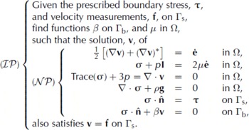
Assume the ice sheet occupies a volume, Ω, of known shape, as shown in Figure 1, bounded by a surface, Γ_s, where we have observations, and a surface, Γ_b, where we wish to solve for the coefficient that linearly relates stresses on the boundary to velocities there, i.e. the parameter in a Robin-type boundary condition. Using Cartesian coordinates, ( x, y, z), denote the outward normal vector on both surfaces by , the material velocity by v, strain-rate tensor by , stress tensor by σ, and pressure by p ≡ −Trace(σ) /3. For now, assume an incompressible material, so that ∇ · v = 0, and a linear viscous rheology, so deviatoric stress is given by , with identity I, and viscosity μ. Further assuming a constant density, ρ, and gravitational field, g, the momentum-conservation equation corresponding to force balance can be written ∇ · σ+ ρg = 0.

Fig. 1.

Geometric depiction of the problem. The ice volume, Ω, has known shape. Measurements of the surface velocity and the stress are available on Γ_s (red dotted). On the rest of the boundary, Γ_b (blue dashed), including the impenetrable part, Γ_i, stresses are defined by a Robin-type boundary condition, with unknown Robin coefficient, β. The viscosity, μ, within Ω is also unknown. We seek solutions for β on Γ_b, and μ within Ω, so that velocities and stresses on Γ_s are consistent with the observational data.

To begin with, consider a simplified problem, in which the force per unit area on the boundary, Γ_b, acts in the opposite direction to the velocity, and in proportion to it, so that , with β > 0, a scalar that may vary spatially; this relationship defines the Robin boundary condition. Later we can adapt this to the more realistic case of sliding past an impenetrable boundary, Γ_i, that supports normal and tangential stresses, such as the base of the ice sheet, but for now we ignore the distinction between Γ_i and the rest of Γ_b.

For the simplified problem the initialization consists of selecting viscosity, μ, in the interior of the domain, and the Robin parameter, β, on the boundary. The inverse Robin problem can be stated as follows:

(1)

We assume the availability of an ice-sheet model, optimized for the efficient solution of the Neumann problem , and that this model can also be used to solve a Dirichlet problem , forced by the surface velocity measurements, f:

(2)

Writing the solutions of the Dirichlet and Neumann problems and as and , p ^N], respectively, the Appendix shows that the inverse problem can be solved by minimizing the Reference Kohn and VogeliusKohn and Vogelius (1984) cost function

(3)

in which the subscript ‘F’ denotes the Frobenius norm, as defined in the Appendix. Furthermore, the gradient of this cost function, with respect to the parameters μ and β, can be expressed as a Gâteaux, or directional, derivative (e.g. Reference ZornZorn, 1946), defined by dJ ≡ d _μJ + d _βJ, with

(4)

where ε is a small parameter that tends to zero in the limit. A more realistic case is that some part of the boundary, Γ_b, is impenetrable, such as the base of the ice sheet. On the impenetrable part, Γ_i, conditions of zero normal velocity, and tangential shear stress proportional to velocity, can be applied:

(5)

Repeating the analysis with this boundary condition, the product of normal forces and normal velocities vanishes in surface integrals over Γ_i, and the results are identical to Equations (3) and (4). Thus, the inverse Robin problem for the case of sliding past an impenetrable boundary can be solved by minimizing J, defined by Equation (3), subject to constraints and , as modified by Equation (5). Furthermore, Equation (4) continues to provide the Gâteaux derivative of J in that case.

Methods

By analogy with the investigation of the Laplace equation, described by Reference Chaabane and JaouaChaabane and Jaoua (1999), the above theory suggests an iterative descent algorithm for minimizing J, and hence selecting μ and β:

(6)

To clarify the above notation, at Step 5 the estimated viscosity, μ, is reduced by an amount , where the strain-rate tensors, and , are available from the Dirichlet and Neumann simulations, respectively.

Results

For the purpose of illustration, consider the following simple application of Algorithm 1, estimating the basal drag coefficient, β, and viscosity, μ, for an infinite slab of constant thickness, h, sliding down an impenetrable, inclined plane at angle α from the horizontal. Define tilted rectangular coordinates so the x- and y-axes are within the plane (in the down- and across-slope directions, respectively) and the z-axis is normal to the plane, increasing upwards. Then neglect all variation in x and y. For observational constraints, specify the downslope surface velocity, f, in the x direction and that the shear stress, σ_xz = μ∂_zv, vanishes at the surface. For this problem the Neumann and Dirichlet problems are second-order, 1-D, boundary-value problems, and can be written in nondimensional form by defining scales |z| = h, |v| = f, |τ| = ρgh sin α, |μ| = |τ| h/f, |β| = |τ| /f. In these units, conservation of momentum in the x direction gives

(7)

where unlabelled equations correspond to both Dirichlet and Neumann problems. Further assuming no variation of μ within the slab, so the parameter space defined by μ and β is two-dimensional, the cost function, J, can be plotted. Figure 2 shows the cost function. This was obtained by numerically solving the boundary-value problems and (Equation (7)) for regularly spaced μ and β (using MATLAB routine bvp4c; Reference Kierzenka and ShampineKierzenka and Shampine, 2001), then evaluating J using Equation (3). The figure also shows the result of applying Algorithm 1, from various initial estimates, with the boundary-value problems solved numerically at each step of the algorithm.

Fig. 2.

Results of applying Algorithm 1 to retrieve the viscosity, μ, and basal drag coefficient, β, for shear flow down an inclined plane. Crosses show the iterative path taken to minimize the cost function, J( μ, β), from various initial estimates. The coloured contours show log₁₀ J. The white dashed curve shows the analytical solution β = 2μ/(2μ − 1). In general, no unique solution is obtained unless an independent estimate of μ or β is available. Circles show two such examples, constrained by prior estimates μ = 1.8 and β = 1.7.

In a more realistic application, with multiple dimensions, it would be impractical to plot the cost function, and specialized numerical algorithms for solving the full Stokes system, or some approximation to it, would be employed in the descent algorithm. Nevertheless, this simple example illustrates the main features of the method.

In fact, the above example can be integrated directly, to reveal that there is no unique solution for nondimensional μ and β which solves the inverse problem , but rather a locus of solutions defined by β = 2μ/(2μ − 1). This locus is shown as a white dashed curve in Figure 2. As anticipated from the theory, it corresponds closely to the minimum of the cost function, and to the solutions converged upon by Algorithm 1.

Figure 2 illustrates that to solve for the drag coefficient, β, prior information about the viscosity, μ, is required. Similarly, to solve for μ requires prior information about β. Nevertheless, if μ (or β) is already known, perhaps from laboratory experiments, Algorithm 1 can be used to determine the other, by setting the initial estimate μ ₀ (or β ₀) to the known value, and the corresponding descent parameter α_μ (or α_β ) to zero: examples are shown in Figure 2.

A more realistic test of the algorithm is shown in Figure 3. This shows a synthetic inversion in a 3-D setting, with nonlinear viscosities for both ice and basal sediment (till). Synthetic data were generated using a commercial Stokes solver to simulate flow down an ice stream 100 km long, 30 km wide and 1.6 km thick, over an isolated patch of low-viscosity till (Fig. 3a). The slope was 0.01 with elevation decreasing in the x direction, driving flow from left to right in Figure 3.

Fig. 3.

Results of applying Algorithm 1 to retrieve the rate coefficient for a nonlinear sliding law in a 3-D simulation. A commercial solver for the Stokes equations was used in this inversion. Each panel represents an ice stream (100 km × 30 km) flowing from left to right over a patch of lower-viscosity sediment. (a) The specified rate coefficient (m d⁻¹ kPa ⁻³); (b) the rate coefficient recovered from noise-free synthetic observations that would be available at the surface; (c) the rate coefficient recovered from synthetic surface observations with random noise added to represent measurement errors after 9 iteration steps and (d) after 19 iterations.

Ice rheology was prescribed by a nonlinear Glen flow law with n = 3 and rate constant A = 4.6 × 10⁻¹⁰ d⁻¹ kPa⁻³. The upper surface was stress-free in all Neumann computations. Periodic boundary conditions were applied at the horizontal boundaries. At the base, a Weertman-type nonlinear sliding law, , with m = 3 was used, with τ _b representing basal shear stress and v _b the basal flow speed.

The coefficient C was specified by adding a Gaussian perturbation to a constant background level (Fig. 3a). This perturbation, centred on x = 50 km, y = 15 km, had amplitude equal to the background value (5.3 × 10⁻⁷ m d⁻¹ kPa⁻³), so that C is double the background value at its peak, with an e-fold decay radius of 5 km.

The rate coefficient, C, was then recovered by applying Algorithm 1, using only those data available at the surface. In this experiment, A is assumed known, and no attempt is made to recover a spatially varying viscosity in the interior. The initial guess for C was spatially uniform at the unperturbed background value. The rate coefficient at each location was updated iteratively, from C_n to C_{n +1}, by adding a contribution in the direction that reduces the cost function. Because an increase in C in effect corresponds to a reduction in β, a change of sign was made to Step 6 of Algorithm 1, replacing it as follows: , with α_C > 0. The basal velocity vectors, and , were from the Dirichlet and Neumann computations, respectively, and their Frobenius norms are simply their magnitude.

If the step-size parameter, α_C , is too large, there is a risk of overshooting the minimum, even if the search direction points locally downhill. We set α_C = 10⁻⁷ m⁻¹ day kPa⁻³, but if a step failed to reduce the cost function, α_C was halved and another trial step taken. If this second step failed, the value of α_C minimizing J in the current search direction was estimated from a quadratic fit, and C_{n +1} updated using this value.

The extension of our theory to the nonlinear sliding law is heuristic, since we have not differentiated the cost function appropriate to the nonlinear case. Despite this, it works well in practice. Results of the inversion are shown in Figure 3b. The close match to Figure 3a demonstrates the successful convergence of the algorithm, even for a 3-D problem with nonlinear rheologies of ice and till.

We investigated the effect of measurement errors upon the algorithm by perturbing the synthetic surface observations with randomly generated noise, before applying the inversion algorithm. Comparing Figure 3a with Figure 3c shows that the recovered rate coefficients suffer some degradation when measurement errors are present. Nevertheless, the inversion is still able to detect the presence of the low-viscosity sediment.

Comparison of Figure 3c with Figure 3d shows that broad-scale features are recovered first. As iterations are continued, the inversion produces sharper features with higher amplitude. Figure 3d shows that this can eventually produce spurious features, by overfitting to measurement errors.

To avoid overfitting, a stopping criterion is needed. For a similar problem Reference Maxwell, Truffer, Avdonin and StueferMaxwell and others (2008) propose a heuristic criterion based upon the mismatch between Neumann and observed velocities at the surface. Our calculations provide support for this approach. Figure 4 shows the root-mean-square (rms) mismatch between the surface velocity data, f, and the surface velocities computed from the Neumann problem . For the noise-free test case, the mismatch decreases iteration by iteration. However, when noise is added, the mismatch stagnates at a level consistent with the rms noise level (dashed horizontal line). Thus, a conservative estimate of the observational error on f can serve to define a stopping criterion. As an example, the first iteration to reach the rms noise level is plotted in Figure 3c.

Fig. 4.

Convergence for synthetic inversions shown in Figure 3. The plot shows the rms mismatch (m d⁻¹) between Neumann and observed surface velocities. Without measurement errors, convergence continues throughout. When measurement errors are introduced, by adding noise to the synthetic data, the convergence stagnates and a stopping criterion is needed. The horizontal dashed line shows the rms of the added noise. Large symbols show the iterations plotted in Figure 3.

Discussion and Conclusions

For the purpose of initializing ice-sheet forecasts, we have described a simple algorithm to invert for the basal drag coefficient and ice viscosity.

If Algorithm 1 is used to estimate the basal drag coefficient and /or refine the ice viscosity, the ice-sheet forecast will begin in a state of force balance, with present-day geometry and surface velocities. This is preferable to a state beginning with present geometry, but with unrealistic viscosity or drag coefficient, since this would produce an ‘initialization shock’ at the beginning of the forecast and a spurious contribution to the sea-level forecast.

Use of Algorithm 1 is also preferable to selecting an initial state for a 21st-century simulation simply by ‘spinning up’ the ice-sheet model over many thousands of years. An ice-sheet model may have more than a million variables describing its geometry and flow. Without the constraint of observations, there is slim chance of obtaining initial conditions close enough to the present-day values to be useful for prediction.

A practical advantage of Algorithm 1 is its ease of implementation. It only uses the forward solver of the Stokes equations, so there is no requirement to develop and test a separate adjoint model. This also means that Algorithm 1 benefits automatically from any parallelization, adaptive grid refinement or asymptotic approximations employed by the forward model. Conveniently, the terms in Equation (4) are proportional to deformational and frictional heating rates, which are routinely evaluated in many ice-sheet models.

This preliminary investigation does not present an exhaustive test of the ability of Algorithm 1 to recover viscosity and basal drag coefficient from realistic glaciological data. In particular, we have assumed that continuous fields of surface elevation, surface velocity and thickness are available. For some applications, error-prone surface velocity data could be incompatible with incompressibility, perhaps leading the Dirichlet problem to be ill-posed unless this constraint is enforced. If the geometry of the bed is poorly known it would be preferable to solve for bed elevation and drag coefficient simultaneously (Reference Gudmundsson and RaymondGudmundsson and Raymond, 2008; Reference Raymond and GudmundssonRaymond and Gudmundsson, 2009). This would require modification of our algorithm, and it may be necessary to take account of prior knowledge of the spatial statistics for bed elevation and its uncertainty (Reference Raymond and GudmundssonRaymond and Gudmundsson, 2009).

To speed convergence, a more sophisticated algorithm, such as conjugate gradients, could be used to minimize the cost function. Deriving the precise derivative of the cost function appropriate for the nonlinear sliding law may also improve the performance. The sensitivity to the stopping criterion suggests that it would be helpful to optimize this aspect further.

Reference Chaabane and JaouaChaabane and others (1999) present a more complete theoretical analysis for the Laplace equation. It would be worth considering which of their results transfer to the glaciological situation considered here. The application to a vector velocity field represents a qualitative difference from the scalar Laplace equation. In particular, further theoretical and numerical work is needed to establish the resolving power of the method, the sensitivity to measurement errors and whether additional regularization is needed. Nevertheless, we hope the inverse Robin problem specified above, the descent algorithm and the preliminary results, will motivate further numerical and theoretical calculations of this kind, so that simulations of 21st-century climate can be undertaken with properly initialized ice-sheet models.