


1. Introduction
In recent decades, wind turbines have grown significantly in size. This trend is expected to continue, especially in the offshore sector, as the wind energy industry seeks to improve the economics of wind turbines (Enevoldsen & Xydis Reference Enevoldsen and Xydis2019; Bilgili & Alphan Reference Bilgili and Alphan2022). However, the increasing size and hub height of wind turbines introduce new research challenges, particularly in understanding and modelling atmospheric turbulence at rotor-relevant altitudes (Veers et al. Reference Veers2023). For example, the widely used Mann (Reference Mann1994) and Kaimal (Kaimal et al. Reference Kaimal, Wyngaard, Izumi and Coté1972) models, recommended by the International Electrotechnical Commission (IEC) for wind turbine design and certification (IEC 2019), were originally developed for turbulence within the atmospheric surface layer. Their validity at the heights of multi-megawatt turbines remains uncertain, partly due to the scarcity of experimental data on turbulence above 100 m in the marine atmospheric boundary layer (MBL) (van Kuik et al. Reference van Kuik2016; Veers et al. Reference Veers2023).
This study aims to present measurements of one-point auto-spectra and two-point spectral coherence of turbulence at heights from 150 to 250 m above sea level, which are then compared with the predictions of the Mann model and its extension, the Syed–Mann model (Syed & Mann Reference Syed and Mann2024). We also attempt to answer the following question: What physical mechanism causes the measurements to deviate from the theoretical foundations of the aforementioned models?
Measurements of atmospheric turbulence over water began with the use of anemometers placed 10–15 m above the surface (Weiler & Burling Reference Weiler and Burling1967; Miyake, Stewart & Burling Reference Miyake, Stewart and Burling1970) and air plane flights (Lenschow & Agee Reference Lenschow and Agee1976; Nicholls & Readings Reference Nicholls and Readings1981; Gage & Nastrom Reference Gage and Nastrom1986) that covered higher altitudes but only provided pointwise measurements over limited durations. Data on the spatio-temporal structure of turbulence in the MBL became more widely available in the 1990s as met-masts were deployed near the coast and offshore (Mann, Kristensen & Courtney Reference Mann, Kristensen and Courtney1991; Gjerstad et al. Reference Gjerstad, Aasen, Andersson, Brevik and Løvseth1995; Vincent et al. Reference Vincent, Larsén, Larsen and Sørensen2013; Larsén et al. Reference Larsén, Vincent and Larsen2013; Holtslag et al. Reference Holtslag, Beirbooms and van Bussel2015; Cheynet, Jakobsen & Reuder Reference Cheynet, Jakobsen and Reuder2018). One of the first campaigns to measure two-point cross-spectra in the marine boundary layer was done by Mann et al. (Reference Mann, Kristensen and Courtney1991) that used two meteorological masts placed on the island of Sprogø in the Great Belt. This dataset was used in the validation of the Mann model. Gjerstad et al. (Reference Gjerstad, Aasen, Andersson, Brevik and Løvseth1995) used measurements spanning many hours from an islet in the Norwegian Sea and observed the spectral gap (van der Hoven Reference van der Hoven1957) in agreement with the seminal Kansas experiment (Kaimal et al. Reference Kaimal, Wyngaard, Izumi and Coté1972). Vincent et al. (Reference Vincent, Larsén, Larsen and Sørensen2013) and Larsén et al. (Reference Larsén, Vincent and Larsen2013) analysed spectra, cross-spectra and coherence at low frequencies down to 10 $^{-6}$
Hz and at separations of more than one kilometre from two wind farms in the North and Baltic Seas. They found that mesoscale turbulence under stationary conditions was two-dimensional (two components of space and two components of velocity, 2D2C) and isotropic such that both components had the same variance. Larsén et al. (Reference Larsén, Larsen and Petersen2016) subsequently derived an empirical expression for the auto-spectra over mesoscales and synoptic scales in the frequency domain, akin to the relation first presented by Lindborg (Reference Lindborg1999) in the wavenumber domain. In another study (Larsén et al. Reference Larsén, Larsen, Petersen and Mikkelsen2021), a similar expression was derived for the cross-wind fluctuations. Cheynet et al. (Reference Cheynet, Jakobsen and Reuder2018) also computed the spectra and vertical coherence over different stability regimes at heights up to 81 m above the German North Sea. They found that the Kaimal model agreed with the observed spectra, except under very stable conditions when there was a spectral gap present. Vertical coherence was also adequately described by the Davenport model (Davenport Reference Davenport1961).
$^{-6}$
Hz and at separations of more than one kilometre from two wind farms in the North and Baltic Seas. They found that mesoscale turbulence under stationary conditions was two-dimensional (two components of space and two components of velocity, 2D2C) and isotropic such that both components had the same variance. Larsén et al. (Reference Larsén, Larsen and Petersen2016) subsequently derived an empirical expression for the auto-spectra over mesoscales and synoptic scales in the frequency domain, akin to the relation first presented by Lindborg (Reference Lindborg1999) in the wavenumber domain. In another study (Larsén et al. Reference Larsén, Larsen, Petersen and Mikkelsen2021), a similar expression was derived for the cross-wind fluctuations. Cheynet et al. (Reference Cheynet, Jakobsen and Reuder2018) also computed the spectra and vertical coherence over different stability regimes at heights up to 81 m above the German North Sea. They found that the Kaimal model agreed with the observed spectra, except under very stable conditions when there was a spectral gap present. Vertical coherence was also adequately described by the Davenport model (Davenport Reference Davenport1961).
The construction costs of offshore met-masts are high and they tend to rise sharply with the height of the mast. Consequently, offshore masts taller than 100 m are rare. This has led to remote sensing techniques such as light detection and ranging (lidar) (Sathe & Mann Reference Sathe and Mann2013) becoming increasingly common in measuring turbulence at higher altitudes in the MBL (Cheynet et al. Reference Cheynet, Jakobsen, Snæbjörnsson, Mikkelsen, Sjöholm, Mann, Hansen, Angelou and Svardal2016, Reference Cheynet2021; Angelou et al. Reference Angelou, Mann and Dubreuil-Boisclair2023; Syed & Mann Reference Syed2024). For instance, short-range dual lidars were deployed by Cheynet et al. (Reference Cheynet, Jakobsen, Snæbjörnsson, Mikkelsen, Sjöholm, Mann, Hansen, Angelou and Svardal2016) on a bridge in Norway at a height of 55 m to measure lateral coherence, demonstrating that spatial averaging effects of lidars were negligible for coherence measurements. Building on this, Cheynet et al. (Reference Cheynet2021) used long-range scanning lidars to record spectra and lateral coherence up to 130 m above the Norwegian Sea. However, high uncertainty in beam pointing directions limited the accuracy of their results. More recently, Angelou et al. (Reference Angelou, Mann and Dubreuil-Boisclair2023) and Syed & Mann (Reference Syed2024) used forward-looking nacelle lidars to measure lateral coherence at separations up to 100 m. These studies also observed mesoscale turbulence with the characteristic $-5/3$
slope (Lindborg Reference Lindborg1999; Larsén et al. Reference Larsén, Larsen and Petersen2016) at wavenumbers below 10
$-5/3$
slope (Lindborg Reference Lindborg1999; Larsén et al. Reference Larsén, Larsen and Petersen2016) at wavenumbers below 10 $^{-3}$
m
$^{-3}$
m $^{-1}$
. However, the measurements were limited to line-of-sight components. Thus, the lateral coherence of the true wind components has not been measured before at separations between 100 to 250 m, at heights above100 m and for frequencies down to the mesoscale range. Consequently, the validity of turbulence models like the Mann model, at these heights and separations, has remained an open question.
$^{-1}$
. However, the measurements were limited to line-of-sight components. Thus, the lateral coherence of the true wind components has not been measured before at separations between 100 to 250 m, at heights above100 m and for frequencies down to the mesoscale range. Consequently, the validity of turbulence models like the Mann model, at these heights and separations, has remained an open question.
In this study we present novel observations of spectra and lateral coherence at heights between 150 and 250 m above the Danish North Sea, with lateral separations of up to 241 m. Our set-up consists of five lidars deployed along the west coast of Denmark, with beam pointing directions calibrated using drones to achieve high accuracy (Thorsen, Simon & Clausen Reference Thorsen, Simon and Clausen2023). This set-up enables direct measurement of the true along-wind and cross-wind components of turbulence. The observations are also compared with the Mann model and its extension, which includes mesoscale turbulence (Syed & Mann Reference Syed and Mann2024). The Syed–Mann model can capture most features of atmospheric turbulence at these heights, albeit with exceptions.
The paper is organised as follows: § 2 describes the site, instrumentation, data processing methods and estimation of atmospheric stability using Weather Research and Forecast (WRF) simulations and boundary layer height detection. Section 3 presents a comparison between our measurements and the turbulence models, with a detailed analysis of cases where discrepancies occur. Finally, key conclusions are summarised in § 4.
2. Experimental dataset
2.1. Description of the field campaign
The experimental site was located near Trans, a small town in the Jutland peninsula on the west coast of Denmark. The site provided unobstructed access to the North Sea while being near the Test Centre Høvsøre where full-scale wind turbine prototypes are routinely tested. Consequently, technicians from the test facility could regularly carry out maintenance on the equipment. Moreover, this region and its climate are of high relevance to wind energy as many offshore wind farms are in operation, under construction or being planned in the North Sea.
We used five long-range pulsed coherent Doppler lidars in the experiment as described in table 1. The campaign lasted for five months, from late January to late June 2024. Thus, the campaign covered a period from late winter to early summer. The change in seasons had a direct effect on the observed atmospheric stability, which is discussed in § 2.3. The set-up of the experiment is shown in figure 1. Two lidars were present at the northern site close to the lighthouse of Bovbjerg while the remaining three lidars were next to the church of Trans in the south. Pictures from these sites are shown in figure 2. The lidar beams had a low elevation angle and intersected approximately 1.5 km from the coast. The plane of intersection lay approximately 150 m above the sea surface from the start of the campaign to the end of April. Subsequently, the elevation angles were increased to move the plane of intersection to nearly 250 m above the sea surface. The azimuth and elevation of the beams during the two periods are described in table 2. Figure 3 provides a closer look at the plane of intersection and the six crossing points. This set-up bears some similarity to the RUNE experiment (Floors et al. Reference Floors, Peña, Lea, Vasiljević, Simon and Courtney2016) that was carried out at the same location, although with only one pair of dual lidars.
Details of the instruments used in the measurement campaign. From left to right the columns are: name of the lidar, manufacturer and model, closest landmark, positions in UTM zone 32V and the elevation above the sea surface of the ground where the lidars are located.

Three-dimensional (3D) view of the experiment indicating the two sites, church and lighthouse, where the black lines indicate the lidar beams in configuration 1 and the red dots show the intersection points. The colours indicate the elevation of the surrounding terrain. The easting and northing axes are defined with the origin at 441 000 m and 6 260 000 m, respectively. Thus, the church is present close to easting 446 000 m and northing 6 262 000 m as indicated in table 1. The arrow with the label ‘N’ denotes the direction of true north that corresponds to 0 $^{\circ }$
azimuth. An interactive version of this plot, the associated data and Jupyter notebook can be found (https://www.cambridge.org/S0022112025111038/JFM-Notebooks/files/Figure_1/Make_figure_1.ipynb).
$^{\circ }$
azimuth. An interactive version of this plot, the associated data and Jupyter notebook can be found (https://www.cambridge.org/S0022112025111038/JFM-Notebooks/files/Figure_1/Make_figure_1.ipynb).

Set-up of the lidars in terms of azimuth and elevation of the beams in configurations 1 and 2. The azimuth is defined such that 0 $^\circ$
is north while the elevation is 0
$^\circ$
is north while the elevation is 0 $^\circ$
for a beam oriented parallel to the sea surface.
$^\circ$
for a beam oriented parallel to the sea surface.

Pictures from the church (a) and lighthouse (b) site showing the instruments used in the experiment. Information about the instruments can be found in table 1.

Extensive verifications of the correct pointing positions of the lidars were performed before, during and after the campaign. The primary method of calibration was hard targeting a drone with real time kinematic (RTK) positioning (Thorsen et al. Reference Thorsen, Simon and Clausen2023). We also relied on sea surface levelling and traditional hard target mapping. A detailed description of the campaign can be found in Mann et al. (Reference Mann, Sjöholm, Patel, Thorsen, Simon, Hung and Gottschall2025). Note that the drone-based calibration resulted in an uncertainty of 1 mrad in the azimuth and elevation angles of the lidar beams. This corresponds to an uncertainty of 1 m in the altitudes and separations shown in table 3, which is negligible compared with the separation distances analysed in this study.
2.2. Preparation of lidar data
This section describes the removal of data with excessive noise and the post-processing applied on the leftover data to prepare it for the analysis shown in § 3.
The available lateral separations for coherence measurements along with the height above sea level and direction bins. The columns from left to right are: lateral separation ( $\Delta _y$
), lidar pairs at the two ends, vertical separation in configuration 1 and 2 (
$\Delta _y$
), lidar pairs at the two ends, vertical separation in configuration 1 and 2 ( $\Delta _z$
), average measurement height in configuration 1 and 2 (
$\Delta _z$
), average measurement height in configuration 1 and 2 ( $z_m$
) and the wind direction bins (
$z_m$
) and the wind direction bins ( $\varTheta$
). The numbers in the braces in columns 2 and 3 refer to the intersection points from figure 3. Note that the heights shown here are the mean of the heights of the two crossing points. As the plane of intersection is not horizontal, the crossing points do not lie on the same height.
$\varTheta$
). The numbers in the braces in columns 2 and 3 refer to the intersection points from figure 3. Note that the heights shown here are the mean of the heights of the two crossing points. As the plane of intersection is not horizontal, the crossing points do not lie on the same height.

Top view of the intersection plane of the lidar beams where the numbers denote the crossing points and the beams from the lidars are denoted according to table 1. The arrow with the label ‘N’ indicates the direction of true north.

Doppler lidars measure the component of the velocity field projected along the lidar beam, which is henceforth referred to as the radial velocity, $v_r$
. Since the radial velocity is sampled at a frequency of 1 Hz, it may contain spikes or noise due to low concentrations of aerosols in the atmosphere, dirt and water on the lens, the presence of obstacles in the lidar beam, etc. (Vasiljević et al. Reference Vasiljević, Lea, Courtney, Cariou, Mann and Mikkelsen2016). The 1 Hz data are first segregated into periods of 10 minutes duration and entire 10 min periods are rejected wherein the noise is above a certain threshold. In the literature, noise is often characterised by the carrier-to-noise ratio (CNR) and a threshold that is constant in time is applied to differentiate between reliable and unreliable data. Although this method is simple to implement, it suffers from the drawback that the optimal CNR threshold varies significantly with the site conditions, instrument manufacturer and experimental set-up (Gryning et al. Reference Gryning, Floors, Peña, Batchvarova and Brümmer2016). Thus, in this study, noise was characterised by another metric:
$v_r$
. Since the radial velocity is sampled at a frequency of 1 Hz, it may contain spikes or noise due to low concentrations of aerosols in the atmosphere, dirt and water on the lens, the presence of obstacles in the lidar beam, etc. (Vasiljević et al. Reference Vasiljević, Lea, Courtney, Cariou, Mann and Mikkelsen2016). The 1 Hz data are first segregated into periods of 10 minutes duration and entire 10 min periods are rejected wherein the noise is above a certain threshold. In the literature, noise is often characterised by the carrier-to-noise ratio (CNR) and a threshold that is constant in time is applied to differentiate between reliable and unreliable data. Although this method is simple to implement, it suffers from the drawback that the optimal CNR threshold varies significantly with the site conditions, instrument manufacturer and experimental set-up (Gryning et al. Reference Gryning, Floors, Peña, Batchvarova and Brümmer2016). Thus, in this study, noise was characterised by another metric: $\sigma _{v_r}$
, which is the standard deviation of
$\sigma _{v_r}$
, which is the standard deviation of $v_r$
over an interval of 10 minutes. The optimal threshold for
$v_r$
over an interval of 10 minutes. The optimal threshold for $\sigma _{v_r}$
was independent of the aforementioned factors.
$\sigma _{v_r}$
was independent of the aforementioned factors.
When $\sigma _{v_r}$
was greater than 4 ms
$\sigma _{v_r}$
was greater than 4 ms $^{-1}$
, the 10 min period contained at least 60 spikes in the 1 Hz data (which corresponds to 10 % of the data). This relation was determined empirically by analysing a large portion of the raw dataset. Consequently, the corresponding 10 min periods were removed from the dataset. On the other hand, when
$^{-1}$
, the 10 min period contained at least 60 spikes in the 1 Hz data (which corresponds to 10 % of the data). This relation was determined empirically by analysing a large portion of the raw dataset. Consequently, the corresponding 10 min periods were removed from the dataset. On the other hand, when $\sigma _{v_r}$
was less than 1.2 ms
$\sigma _{v_r}$
was less than 1.2 ms $^{-1}$
, the 10 min period was free from spikes and was retained for further post-processing. When
$^{-1}$
, the 10 min period was free from spikes and was retained for further post-processing. When $1.2 \leqslant \sigma _{v_r} \leqslant 4$
, the method developed by Beck & Kühn (Reference Beck and Kühn2017) was used to remove spikes. It is based on 2D Gaussian kernel density estimation (KDE) using
$1.2 \leqslant \sigma _{v_r} \leqslant 4$
, the method developed by Beck & Kühn (Reference Beck and Kühn2017) was used to remove spikes. It is based on 2D Gaussian kernel density estimation (KDE) using $v_r$
and CNR and relies on the assumption that good data are self-similar. As a result, they must be present in ‘data-dense’ regions in the abstract space defined by
$v_r$
and CNR and relies on the assumption that good data are self-similar. As a result, they must be present in ‘data-dense’ regions in the abstract space defined by $v_r$
and CNR. Beck & Kühn (Reference Beck and Kühn2017) found that the method minimises the mean error between lidar and sonic anemometer measurements as compared with many other commonly used spike-removal algorithms. The method was modified such that it estimated the kernel density of radial velocity differences (
$v_r$
and CNR. Beck & Kühn (Reference Beck and Kühn2017) found that the method minimises the mean error between lidar and sonic anemometer measurements as compared with many other commonly used spike-removal algorithms. The method was modified such that it estimated the kernel density of radial velocity differences ( $\Delta v_r$
instead of
$\Delta v_r$
instead of $v_r$
) and the CNR as this reduced the amount of data incorrectly identified as noise. After applying the modified KDE algorithm, if less than 10 % of the data was lost in a given 10 min period or the spike removal left gaps less than 5 s in duration, then the gaps were filled by linear interpolation. Otherwise, the corresponding 10 min period was removed as well. Note that the spike-removal algorithm did not remove all the spikes in the dataset. The leftover noise is dealt with separately as described in the next section.
$v_r$
) and the CNR as this reduced the amount of data incorrectly identified as noise. After applying the modified KDE algorithm, if less than 10 % of the data was lost in a given 10 min period or the spike removal left gaps less than 5 s in duration, then the gaps were filled by linear interpolation. Otherwise, the corresponding 10 min period was removed as well. Note that the spike-removal algorithm did not remove all the spikes in the dataset. The leftover noise is dealt with separately as described in the next section.
Next, the east–west ( $v_{\textit{EW}}$
) and north–south (
$v_{\textit{EW}}$
) and north–south ( $v_{\textit{NS}}$
) wind components were reconstructed at the six crossing points using the following relations (Peña & Mann Reference Peña and Mann2019):
$v_{\textit{NS}}$
) wind components were reconstructed at the six crossing points using the following relations (Peña & Mann Reference Peña and Mann2019):
 \begin{align} \underbrace {\left [\begin{array}{l} v_{r_1} \\ v_{r_2} \end{array}\right ]}_{\mathbf{v_r}}=\underbrace {\left [\begin{array}{cc} \cos \zeta _1 \cos \phi _1 & \sin \zeta _1 \cos \phi _1 \\ \cos \zeta _2 \cos \phi _2 & \sin \zeta _2 \cos \phi _2 \end{array}\right ]}_{\mathbf{M}} \underbrace {\left [\begin{array}{l} v_{\textit{EW}} \\ v_{\textit{NS}} \end{array}\right ]}_{\mathbf{v}} \end{align}
and
 \begin{align} \mathbf{v}=\unicode{x1D648}^{\,{-}1} \mathbf{v_r}. \end{align}
The subscripts 1 and 2 refer to the lidars close to the church and lighthouse, respectively, whereas $\zeta$
is the azimuthal orientation of the beam and
$\zeta$
is the azimuthal orientation of the beam and $\phi$
is its elevation. This relation relies on the assumption that the projection of the vertical wind component along the lidar beam is negligible as compared with the radial wind speed. For instance, if the vertical component,
$\phi$
is its elevation. This relation relies on the assumption that the projection of the vertical wind component along the lidar beam is negligible as compared with the radial wind speed. For instance, if the vertical component, $w$
, is 1 ms
$w$
, is 1 ms $^{-1}$
then its projection along the lidar beam with an elevation angle of 10
$^{-1}$
then its projection along the lidar beam with an elevation angle of 10 $^{\circ }$
is
$^{\circ }$
is $1\sin 10^{\circ } \approx 0.17$
ms
$1\sin 10^{\circ } \approx 0.17$
ms $^{-1}$
. This is about 1.7 % of the radial velocity measurement, if
$^{-1}$
. This is about 1.7 % of the radial velocity measurement, if $v_r = 10$
ms
$v_r = 10$
ms $^{-1}$
. Indeed, the projection of the vertical component along the lidar beam is between
$^{-1}$
. Indeed, the projection of the vertical component along the lidar beam is between $1\,\%\text{-}5\,\%$
of the radial wind velocity measurements for the range of elevation angle analysed in this study (refer table 2). The vertical velocity component also introduces a small bias in the measurements of the auto-spectra. This effect is discussed in more detail in the next section and at the end of Appendix B. Since the beams of the church and lighthouse lidars are approximately 90
$1\,\%\text{-}5\,\%$
of the radial wind velocity measurements for the range of elevation angle analysed in this study (refer table 2). The vertical velocity component also introduces a small bias in the measurements of the auto-spectra. This effect is discussed in more detail in the next section and at the end of Appendix B. Since the beams of the church and lighthouse lidars are approximately 90 $^{\circ }$
apart, when using (2.1) and (2.2), the uncertainty in (2.1) is independent of the wind direction (Peña & Mann Reference Peña and Mann2019). However, reconstructing the horizontal wind requires simultaneous data from both lidars. Data availability after noise removal was not uniform across the five lidars. Some lidars showed noisier data than the rest, probably because they were older models (Sterenn) or had accumulated more dirt on the lens (Chinook). Consequently, the 10 min periods where (2.2) could not be applied were also removed from the dataset.
$^{\circ }$
apart, when using (2.1) and (2.2), the uncertainty in (2.1) is independent of the wind direction (Peña & Mann Reference Peña and Mann2019). However, reconstructing the horizontal wind requires simultaneous data from both lidars. Data availability after noise removal was not uniform across the five lidars. Some lidars showed noisier data than the rest, probably because they were older models (Sterenn) or had accumulated more dirt on the lens (Chinook). Consequently, the 10 min periods where (2.2) could not be applied were also removed from the dataset.
Subsequently, the horizontal wind speed, $u_{\textit{hor}}$
, and wind direction,
$u_{\textit{hor}}$
, and wind direction, $\theta$
, were computed:
$\theta$
, were computed:
 \begin{align} u_{\textit{hor}} = \sqrt {v_{\textit{EW}}^2 + v_{\textit{NS}}^2}, \\[-28pt] \nonumber \end{align}
 \begin{align} \theta = \arctan \left ( -v_{\textit{EW}}, -v_{\textit{NS}} \right ). \\[2pt] \nonumber \end{align}
Note that the wind direction will be expressed in the meteorological convention, where 0 $^\circ$
refers to wind blowing from true north. The histograms of the 10 minute mean horizontal wind speed (
$^\circ$
refers to wind blowing from true north. The histograms of the 10 minute mean horizontal wind speed ( $U_{\textit{hor}}$
) and wind direction (
$U_{\textit{hor}}$
) and wind direction ( $\varTheta$
) are shown in figures 4 and 5, where
$\varTheta$
) are shown in figures 4 and 5, where $z_m$
indicates the measurement height above sea level. The modal 10 min wind speed is between 11 and 12 ms
$z_m$
indicates the measurement height above sea level. The modal 10 min wind speed is between 11 and 12 ms $^{-1}$
. The maximum observed value of
$^{-1}$
. The maximum observed value of $U_{\textit{hor}}$
was 26.2 ms
$U_{\textit{hor}}$
was 26.2 ms $^{-1}$
. The modal wind direction was between 210
$^{-1}$
. The modal wind direction was between 210 $^\circ$
and 220
$^\circ$
and 220 $^\circ$
from the start of the campaign to the end of April 2024. While from May 2024 to the end of the campaign, it was between 290
$^\circ$
from the start of the campaign to the end of April 2024. While from May 2024 to the end of the campaign, it was between 290 $^\circ$
and 300
$^\circ$
and 300 $^\circ$
. This corresponds to westerly circulation over the northern mid-latitudes due to the Ferrel cell. Easterly winds are also frequently observed, but only westerly winds were analysed in this study since the scope is limited to marine atmospheric turbulence.
$^\circ$
. This corresponds to westerly circulation over the northern mid-latitudes due to the Ferrel cell. Easterly winds are also frequently observed, but only westerly winds were analysed in this study since the scope is limited to marine atmospheric turbulence.
The number of 10 min periods, $N$
, for different 10 min mean wind speed bins, computed at crossing point 2 for (a) configuration 1 and (b) configuration 2. The measurement height,
$N$
, for different 10 min mean wind speed bins, computed at crossing point 2 for (a) configuration 1 and (b) configuration 2. The measurement height, $z_m$
, is shown at the top of each figure. The data used in the final analysis are highlighted in blue.
$z_m$
, is shown at the top of each figure. The data used in the final analysis are highlighted in blue.

The number of 10 min periods, $N$
, for different 10 min mean wind direction bins plotted in polar coordinates and computed at crossing point 2 for (a) configuration 1 and (b) configuration 2. The measurement height,
$N$
, for different 10 min mean wind direction bins plotted in polar coordinates and computed at crossing point 2 for (a) configuration 1 and (b) configuration 2. The measurement height, $z_m$
, is shown at the top of each figure. The data used in the final analysis are highlighted in blue.
$z_m$
, is shown at the top of each figure. The data used in the final analysis are highlighted in blue.

This study aims to compare the measurements with the turbulence models down to frequencies lower than 10 min $^{-1}$
, similar to the work of Cheynet et al. (Reference Cheynet, Jakobsen and Reuder2018), Larsén et al. (Reference Larsén, Vincent and Larsen2013, Reference Larsén, Larsen and Petersen2016) and Syed & Mann (Reference Syed and Mann2024). Due to the scanning configuration of one of the lidars (Zonda), the duration of the longest continuous time series that can be reconstructed is 20 min. Consequently, from the dataset retained after the aforementioned data removal steps, we found two contiguous 10 min periods. These were attached to each other to create a time series that was 20 min in duration.
$^{-1}$
, similar to the work of Cheynet et al. (Reference Cheynet, Jakobsen and Reuder2018), Larsén et al. (Reference Larsén, Vincent and Larsen2013, Reference Larsén, Larsen and Petersen2016) and Syed & Mann (Reference Syed and Mann2024). Due to the scanning configuration of one of the lidars (Zonda), the duration of the longest continuous time series that can be reconstructed is 20 min. Consequently, from the dataset retained after the aforementioned data removal steps, we found two contiguous 10 min periods. These were attached to each other to create a time series that was 20 min in duration.
In this experiment, coherence was measured between the lateral separations, $\Delta _y$
, whose values are shown in table 3. Note that (3.5), (3.10) and (3.15) were used to quantify the coherence. The separations were obtained by selecting two intersection points from figure 3. The respective intersection points are shown in the second and third columns of table 3. For example, points 6 and 5 were horizontally separated by 50 m while the vertical separation (
$\Delta _y$
, whose values are shown in table 3. Note that (3.5), (3.10) and (3.15) were used to quantify the coherence. The separations were obtained by selecting two intersection points from figure 3. The respective intersection points are shown in the second and third columns of table 3. For example, points 6 and 5 were horizontally separated by 50 m while the vertical separation ( $\Delta _y$
) was 4.5 m and 9 m in configurations 1 and 2, respectively. Moreover, the lateral coherence in this case was only computed for those 20-min periods where the mean wind direction (
$\Delta _y$
) was 4.5 m and 9 m in configurations 1 and 2, respectively. Moreover, the lateral coherence in this case was only computed for those 20-min periods where the mean wind direction ( $\varTheta$
) was between 281
$\varTheta$
) was between 281 $^{\circ }$
and 341
$^{\circ }$
and 341 $^{\circ }$
. Since the analysis is now focused on 20-minute periods, the mean wind direction is also computed over a duration of 20 min. The wind direction bins shown in table 3 were obtained by considering a 30
$^{\circ }$
. Since the analysis is now focused on 20-minute periods, the mean wind direction is also computed over a duration of 20 min. The wind direction bins shown in table 3 were obtained by considering a 30 $^{\circ }$
interval around the normal to the separation vector connecting the intersection points. The 20-min periods where the mean wind direction was outside these bins were also removed from the dataset. Measuring coherence also requires simultaneous data from both intersection points. As mentioned before, data from Sterenn and Chinook was noisier than data recorded by the other lidars. Thus, these two lidars had lower data availability after removal of noisy data based on
$^{\circ }$
interval around the normal to the separation vector connecting the intersection points. The 20-min periods where the mean wind direction was outside these bins were also removed from the dataset. Measuring coherence also requires simultaneous data from both intersection points. As mentioned before, data from Sterenn and Chinook was noisier than data recorded by the other lidars. Thus, these two lidars had lower data availability after removal of noisy data based on $\sigma _{v_r}$
and the modified KDE algorithm. Similarly, the data availability was lower at points 4, 5 and 6 compared with the rest. Thus, for a given separation, the 20-minute periods where simultaneous data from both points were not available were also discarded.
$\sigma _{v_r}$
and the modified KDE algorithm. Similarly, the data availability was lower at points 4, 5 and 6 compared with the rest. Thus, for a given separation, the 20-minute periods where simultaneous data from both points were not available were also discarded.
Turbulence is often analysed in the coordinate system where the $x$
axis is aligned with the mean wind direction, which varies in time and with height. Thus, the along-wind (
$x$
axis is aligned with the mean wind direction, which varies in time and with height. Thus, the along-wind ( $u$
) and cross-wind (
$u$
) and cross-wind ( $v$
) components are computed as
$v$
) components are computed as
 \begin{align} u = u_{\textit{hor}} \cos \left ( \theta - \varTheta \right ), \\[-28pt] \nonumber \end{align}
 \begin{align} v = u_{\textit{hor}} \sin \left ( \theta - \varTheta \right ) , \\[-2pt] \nonumber\end{align}
where $\varTheta$
is the 20 min mean wind direction during a particular period in time and at the height where the time series of
$\varTheta$
is the 20 min mean wind direction during a particular period in time and at the height where the time series of $u_{\textit{hor}}$
and
$u_{\textit{hor}}$
and $\theta$
were measured. The analysis is also limited to data that is quasi-stationary. A linear fit (Angelou et al. Reference Angelou, Mann and Dubreuil-Boisclair2023) was computed to each 20 min time series and if the slope was greater than 2 ms
$\theta$
were measured. The analysis is also limited to data that is quasi-stationary. A linear fit (Angelou et al. Reference Angelou, Mann and Dubreuil-Boisclair2023) was computed to each 20 min time series and if the slope was greater than 2 ms $^{-1}$
h
$^{-1}$
h $^{-1}$
then that period was rejected. For the final processing step, the data where at least four 20 min periods were present in succession was accepted. This is because each 20 min period is considered as a separate realisation and the auto-spectra and coherence will be averaged over at least four realisations. The data available after each processing step is shown in table 4 and is also highlighted in figures 4 and 5. The 388 periods from table 4 correspond to 50 ensembles. Since these ensembles will be referred to on many occasions in this study, an example of the first ensemble is discussed to explain the terminology and the binning of the processed data. The first ensemble contains data from 20 February 2024 01:00 UTC to 05:00 UTC. This corresponds to 12 samples each of which is 20 minutes long. The ensemble-mean wind direction was 294
$^{-1}$
then that period was rejected. For the final processing step, the data where at least four 20 min periods were present in succession was accepted. This is because each 20 min period is considered as a separate realisation and the auto-spectra and coherence will be averaged over at least four realisations. The data available after each processing step is shown in table 4 and is also highlighted in figures 4 and 5. The 388 periods from table 4 correspond to 50 ensembles. Since these ensembles will be referred to on many occasions in this study, an example of the first ensemble is discussed to explain the terminology and the binning of the processed data. The first ensemble contains data from 20 February 2024 01:00 UTC to 05:00 UTC. This corresponds to 12 samples each of which is 20 minutes long. The ensemble-mean wind direction was 294 $^{\circ }$
while the ensemble-mean wind speed was 12.3 ms
$^{\circ }$
while the ensemble-mean wind speed was 12.3 ms $^{-1}$
. Since the realisations were quasi-stationary, the ensemble mean was representative of the mean wind speed and wind direction of each individual 20 min period. Moreover, the lidars Chinook, Brise and Sterenn recorded data that met the noise criteria defined earlier. Thus, this ensemble contains measurements of the lateral coherence between points 5 and 6 from figure 3 along with the auto-spectra at both the points.
$^{-1}$
. Since the realisations were quasi-stationary, the ensemble mean was representative of the mean wind speed and wind direction of each individual 20 min period. Moreover, the lidars Chinook, Brise and Sterenn recorded data that met the noise criteria defined earlier. Thus, this ensemble contains measurements of the lateral coherence between points 5 and 6 from figure 3 along with the auto-spectra at both the points.
Overview of the processes applied on the raw lidar data to prepare it for the analysis of auto-spectra and lateral coherence. The subsequent data availability summed over all lidars or crossing points is shown in the second column.

2.3. Estimation of atmospheric stability
We aim to assign each of the 50 ensembles to a particular stability group based on the stability parameter, $\xi$
, and the classifications described in table 5. An implicit assumption in the analysis presented herein is that since data are quasi-stationary, time averaging can be replaced by ensemble averaging (Wyngaard Reference Wyngaard2010). Moreover, it must be emphasised that ensembles with the same stability are not binned together. Thus, even if two ensembles belong to the same stability group, they are analysed separately. This prevents averaging out phenomena that might not occur during all periods with the same stability. One such example is shown in § 3.4 where gravity waves are possibly detected during a period of very stable stratification.
$\xi$
, and the classifications described in table 5. An implicit assumption in the analysis presented herein is that since data are quasi-stationary, time averaging can be replaced by ensemble averaging (Wyngaard Reference Wyngaard2010). Moreover, it must be emphasised that ensembles with the same stability are not binned together. Thus, even if two ensembles belong to the same stability group, they are analysed separately. This prevents averaging out phenomena that might not occur during all periods with the same stability. One such example is shown in § 3.4 where gravity waves are possibly detected during a period of very stable stratification.
Stability regimes used to classify the ensembles.

Table 5 is drawn from the stability classes used by Cheynet et al. (Reference Cheynet, Jakobsen and Reuder2018) while $\xi$
is the non-dimensional stability parameter:
$\xi$
is the non-dimensional stability parameter:
 \begin{align} \xi = \left \langle \frac {z_i}{L_{\textit{mo}}} \right \rangle \! . \end{align}
Here, $z_i$
is the height of the boundary layer and
$z_i$
is the height of the boundary layer and $L_{\textit{mo}}$
is the Monin-Obukhov length. The brackets,
$L_{\textit{mo}}$
is the Monin-Obukhov length. The brackets, $\left \langle \boldsymbol{\cdot }\right \rangle$
, represent ensemble averaging. Measurements of
$\left \langle \boldsymbol{\cdot }\right \rangle$
, represent ensemble averaging. Measurements of $z_i$
could be obtained from a ceilometer, however, measuring
$z_i$
could be obtained from a ceilometer, however, measuring $ {1}/{L_{\textit{mo}}}$
was not possible because there were no sonic anemometers present on site (due to logistical and economical constraints). Hence, the Monin–Obukhov length computed by WRF (Skamarock et al. Reference Skamarock, Klemp, Dudhia, Gill, Barker, Wang and Powers2005) simulations was used in the calculation of
$ {1}/{L_{\textit{mo}}}$
was not possible because there were no sonic anemometers present on site (due to logistical and economical constraints). Hence, the Monin–Obukhov length computed by WRF (Skamarock et al. Reference Skamarock, Klemp, Dudhia, Gill, Barker, Wang and Powers2005) simulations was used in the calculation of $\xi$
.
$\xi$
.
While several definitions exist for the boundary layer height (Stull Reference Stull1988), in this study, $z_i$
is defined as the height where the aerosol concentration reduces to its level in the free atmosphere. This is because measurements of the vertical profile of the aerosols in the atmosphere were readily available at the site. A Vaisala CL31 ceilometer was placed next to the church of Trans. It measured the vertical profile of the aerosol backscatter at a sampling interval of 16 s and with a vertical resolution of 10 m. Steyn, Baldi & Hoff (Reference Steyn, Baldi and Hoff1999) showed that under ideal cloudless conditions, the aerosol profile in a well-mixed boundary layer follows the shape of the Gauss error function. Thus, the boundary layer height could be computed by fitting the error function to measurements of the backscatter vertical profile. Note that the backscatter profiles were time averaged over a duration of 10 min to reduce noise and obtain a better fit with the error function. However, when clouds form within the boundary layer, it is not possible to detect
$z_i$
is defined as the height where the aerosol concentration reduces to its level in the free atmosphere. This is because measurements of the vertical profile of the aerosols in the atmosphere were readily available at the site. A Vaisala CL31 ceilometer was placed next to the church of Trans. It measured the vertical profile of the aerosol backscatter at a sampling interval of 16 s and with a vertical resolution of 10 m. Steyn, Baldi & Hoff (Reference Steyn, Baldi and Hoff1999) showed that under ideal cloudless conditions, the aerosol profile in a well-mixed boundary layer follows the shape of the Gauss error function. Thus, the boundary layer height could be computed by fitting the error function to measurements of the backscatter vertical profile. Note that the backscatter profiles were time averaged over a duration of 10 min to reduce noise and obtain a better fit with the error function. However, when clouds form within the boundary layer, it is not possible to detect $z_i$
from a ceilometer (or any laser-based remote sensing method) (Hennemuth & Lammert Reference Hennemuth and Lammert2006) because the cloud absorbs light from the laser and no backscatter is obtained after a certain height within the cloud. In such instances, the height where the backscatter becomes negligible is taken as a rough estimate of
$z_i$
from a ceilometer (or any laser-based remote sensing method) (Hennemuth & Lammert Reference Hennemuth and Lammert2006) because the cloud absorbs light from the laser and no backscatter is obtained after a certain height within the cloud. In such instances, the height where the backscatter becomes negligible is taken as a rough estimate of $z_i$
. The implications of the uncertainty in estimations of
$z_i$
. The implications of the uncertainty in estimations of $z_i$
under cloudy conditions are discussed at the end of this section. We refer the reader to Appendix A for more details of boundary layer height estimation from ceilometer measurements.
$z_i$
under cloudy conditions are discussed at the end of this section. We refer the reader to Appendix A for more details of boundary layer height estimation from ceilometer measurements.
The Monin–Obukhov length was determined from WRF simulations carried out by Olsen et al. (Reference Olsen, Hahmann, de, Alonso, Žagar and Dörenkämper2025) as the measurement site was present within the innermost domain of the simulations. The simulations also covered the entire duration of the campaign. Weather Research and Forecast computes the inverse Monin–Obukhov length ( $ {1}/{L_{\textit{mo}}}$
) using bulk estimates of the heat flux from the temperature difference between the surface and the first model level. This is coupled to the planetary boundary layer scheme (PBL) and Monin–Obukhov similarity theory (Peña & Hahmann Reference Peña and Hahmann2012; Skamarock et al. Reference Skamarock, Klemp, Dudhia, Gill, Barker, Wang and Powers2005). The configuration with the three-dimensional turbulent kinetic energy (3DTKE) PBL from Olsen et al. (Reference Olsen, Hahmann, de, Alonso, Žagar and Dörenkämper2025) was used to obtain estimates of
$ {1}/{L_{\textit{mo}}}$
) using bulk estimates of the heat flux from the temperature difference between the surface and the first model level. This is coupled to the planetary boundary layer scheme (PBL) and Monin–Obukhov similarity theory (Peña & Hahmann Reference Peña and Hahmann2012; Skamarock et al. Reference Skamarock, Klemp, Dudhia, Gill, Barker, Wang and Powers2005). The configuration with the three-dimensional turbulent kinetic energy (3DTKE) PBL from Olsen et al. (Reference Olsen, Hahmann, de, Alonso, Žagar and Dörenkämper2025) was used to obtain estimates of $ {1}/{L_{\textit{mo}}}$
at intervals of 30 min.
$ {1}/{L_{\textit{mo}}}$
at intervals of 30 min.
Since $z_i$
and
$z_i$
and $ {1}/{L_{\textit{mo}}}$
were sampled at different rates (10 min and 30 min, respectively), they were ensemble averaged separately such that
$ {1}/{L_{\textit{mo}}}$
were sampled at different rates (10 min and 30 min, respectively), they were ensemble averaged separately such that
 \begin{align} \xi = \left \langle z_i \right \rangle \left \langle \frac {1}{L_{\textit{mo}}} \right \rangle \! . \end{align}
As an example of stability classification, consider the first ensemble of wind speed measurements. It contains data from 20 February 2024 01:00 UTC to 05:00 UTC. Hence, concurrent data (corresponding to 36 periods of 10 minutes) from the ceilometer were used to determine $\left \langle z_i \right \rangle$
. Similarly, concurrent data (eight samples) were retrieved from the WRF simulations to find
$\left \langle z_i \right \rangle$
. Similarly, concurrent data (eight samples) were retrieved from the WRF simulations to find $ \left \langle {1}/{L_{\textit{mo}}} \right \rangle$
. Since
$ \left \langle {1}/{L_{\textit{mo}}} \right \rangle$
. Since $\xi$
was found to be
$\xi$
was found to be $-0.78$
, this ensemble period was classified as stable (S) according to table 5. The ensemble-averaged value of
$-0.78$
, this ensemble period was classified as stable (S) according to table 5. The ensemble-averaged value of $\xi$
was representative of the stability during the entire ensemble period (which in some cases was 8 hours long), as the individual 20 min periods never showed any abrupt changes in the boundary layer height or the Monin–Obukhov length. Daily variations in stability were also not observed at the experimental site as it is located near shore where the global stability varies on a seasonal basis (Sathe et al. Reference Sathe, Gryning and Peña2011a
). Indeed, stable atmospheric conditions were commonly observed during the period from February to late April while unstable conditions were more frequent from early May till the end of the campaign.
$\xi$
was representative of the stability during the entire ensemble period (which in some cases was 8 hours long), as the individual 20 min periods never showed any abrupt changes in the boundary layer height or the Monin–Obukhov length. Daily variations in stability were also not observed at the experimental site as it is located near shore where the global stability varies on a seasonal basis (Sathe et al. Reference Sathe, Gryning and Peña2011a
). Indeed, stable atmospheric conditions were commonly observed during the period from February to late April while unstable conditions were more frequent from early May till the end of the campaign.
The stability classification based on ceilometer measurements and WRF has two sources of uncertainty. As mentioned previously, accurately determining $z_i$
under cloudy conditions is not possible. In these conditions,
$z_i$
under cloudy conditions is not possible. In these conditions, $z_i$
was estimated as the height at which the backscatter signal was lost within the cloud. This certainly underestimates the actual boundary layer height. The second source of uncertainty is that to our knowledge, the
$z_i$
was estimated as the height at which the backscatter signal was lost within the cloud. This certainly underestimates the actual boundary layer height. The second source of uncertainty is that to our knowledge, the $L_{\textit{mo}}$
from WRF using the 3DTKE scheme has never been validated against measurements. Peña & Hahmann (Reference Peña and Hahmann2012) found that estimates of
$L_{\textit{mo}}$
from WRF using the 3DTKE scheme has never been validated against measurements. Peña & Hahmann (Reference Peña and Hahmann2012) found that estimates of $L_{\textit{mo}}$
from WRF and sonic anemometers were strongly correlated in the near-neutral region but showed considerable scatter for the more extreme stability conditions when using the Yonsei University (YSU) PBL scheme. Both 3DTKE and YSU show similar behaviour (Zhang et al. Reference Zhang, Bao, Chen and Grell2018), for instance, in predicting the potential temperature profile. Consequently, the conclusions of Peña & Hahmann (Reference Peña and Hahmann2012) may also be valid for the 3DTKE scheme. Thus, given these uncertainties, the stability classification of each ensemble was verified with the measured vertical profiles of ensemble-averaged wind speed and direction. Appendix C provides more details along with some examples. While the verification was based on qualitative analysis, wind shear and veer are often strong indicators of stability. Thus, this verification with an independent set of measurements provided sufficient confidence in the stability classification.
$L_{\textit{mo}}$
from WRF and sonic anemometers were strongly correlated in the near-neutral region but showed considerable scatter for the more extreme stability conditions when using the Yonsei University (YSU) PBL scheme. Both 3DTKE and YSU show similar behaviour (Zhang et al. Reference Zhang, Bao, Chen and Grell2018), for instance, in predicting the potential temperature profile. Consequently, the conclusions of Peña & Hahmann (Reference Peña and Hahmann2012) may also be valid for the 3DTKE scheme. Thus, given these uncertainties, the stability classification of each ensemble was verified with the measured vertical profiles of ensemble-averaged wind speed and direction. Appendix C provides more details along with some examples. While the verification was based on qualitative analysis, wind shear and veer are often strong indicators of stability. Thus, this verification with an independent set of measurements provided sufficient confidence in the stability classification.
3. Results
3.1. Description of turbulence models
The measurements of auto-spectra and lateral coherence were compared with the Mann (Reference Mann1994) and Syed & Mann (Reference Syed and Mann2024) models, henceforth referred to as M94 and S24, respectively. The M94 model describes the spatial structure of homogeneous, anisotropic, neutral, surface layer turbulence using rapid distortion theory and a parametrisation of the eddy lifetime. Although Mann (Reference Mann1994) presents two models: uniform shear (US) and uniform shear plus blockage (US + B), only the former is within the scope of this paper. The US model has three parameters: $L$
,
$L$
, $\varGamma$
and
$\varGamma$
and $\alpha \varepsilon ^{({2}/{3})}$
. Here
$\alpha \varepsilon ^{({2}/{3})}$
. Here $L$
is a length scale that is related to the size of the most energetic eddies;
$L$
is a length scale that is related to the size of the most energetic eddies; $\varGamma$
is the anisotropy parameter and defines the lifetime of the eddies. The definition of
$\varGamma$
is the anisotropy parameter and defines the lifetime of the eddies. The definition of $\varGamma$
can be found in Mann (Reference Mann1994, Equation (3.6)). It relates the eddy lifetime to the linear shear that rapidly distorts the initial isotropic von Kármán spectra (von Kármán Reference von Kármán1948) into the anisotropic spectra. Thus, as
$\varGamma$
can be found in Mann (Reference Mann1994, Equation (3.6)). It relates the eddy lifetime to the linear shear that rapidly distorts the initial isotropic von Kármán spectra (von Kármán Reference von Kármán1948) into the anisotropic spectra. Thus, as $\varGamma$
increases, the turbulent eddies live for a longer time and suffer more distortion, resulting in turbulence that is more anisotropic. Finally,
$\varGamma$
increases, the turbulent eddies live for a longer time and suffer more distortion, resulting in turbulence that is more anisotropic. Finally, $\alpha \varepsilon ^{({2}/{3})}$
is a scaling parameter and the level of the inertial subrange in the initial von Kármán spectra. Herein,
$\alpha \varepsilon ^{({2}/{3})}$
is a scaling parameter and the level of the inertial subrange in the initial von Kármán spectra. Herein, $\alpha$
is the spectral Kolmogorov constant and
$\alpha$
is the spectral Kolmogorov constant and $\varepsilon$
is the turbulent energy dissipation rate. These parameters are typically computed by fitting the modelled auto-spectra to the measured auto-spectra. Note that in the equations that follow, there is no summation over repeated indices.
$\varepsilon$
is the turbulent energy dissipation rate. These parameters are typically computed by fitting the modelled auto-spectra to the measured auto-spectra. Note that in the equations that follow, there is no summation over repeated indices.
The modelled auto-spectrum is given by
 \begin{align} F_{i} \left (k_1; L, \varGamma , \alpha \varepsilon ^{\frac {2}{3}} \right ) =\int _{-\infty }^{\infty } \int _{-\infty }^{\infty } \varPhi _{\textit{ii}}\left (\boldsymbol{k}; L, \varGamma , \alpha \varepsilon ^{\frac {2}{3}}\right ) \mathrm{d} k_2 \mathrm{d} k_3, \end{align}
where $F_{i} (k_1 )$
is the auto-spectrum in wavenumber space:
$F_{i} (k_1 )$
is the auto-spectrum in wavenumber space: $\boldsymbol{k} = (k_1, k_2, k_3)$
and
$\boldsymbol{k} = (k_1, k_2, k_3)$
and $\boldsymbol{\varPhi } (\boldsymbol{k} )$
is the spectral tensor derived by Mann (Reference Mann1994). Here the indices 1, 2 and 3 refer to the along-wind (
$\boldsymbol{\varPhi } (\boldsymbol{k} )$
is the spectral tensor derived by Mann (Reference Mann1994). Here the indices 1, 2 and 3 refer to the along-wind ( $u$
), cross-wind (
$u$
), cross-wind ( $v$
) and vertical components (
$v$
) and vertical components ( $w$
), respectively. In general, the spectral tensor is defined as the Fourier transform of the two-point covariance tensor,
$w$
), respectively. In general, the spectral tensor is defined as the Fourier transform of the two-point covariance tensor, $R_{\textit{ij}}(\boldsymbol{r})$
(Lumley Reference Lumley1970):
$R_{\textit{ij}}(\boldsymbol{r})$
(Lumley Reference Lumley1970):
 \begin{align} \varPhi _{\textit{ij}}(\boldsymbol{k})=\frac {1}{(2 \pi )^3} \int R_{\textit{ij}}(\boldsymbol{r}) \exp (-\mathrm{i} \boldsymbol{k} \boldsymbol{\cdot }\boldsymbol{r}) \mathrm{d} \boldsymbol{r} \end{align}
and
 \begin{align} R_{\textit{ij}}(\boldsymbol{r})=\left \langle u_i(\boldsymbol{x}) u_{\kern-1pt j}(\boldsymbol{x}+\boldsymbol{r})\right \rangle . \end{align}
Here, $\left \langle \boldsymbol{\cdot }\right \rangle$
denotes ensemble averaging and
$\left \langle \boldsymbol{\cdot }\right \rangle$
denotes ensemble averaging and $\boldsymbol{r}$
is the separation vector.
$\boldsymbol{r}$
is the separation vector.
The components of the spectral tensor can be calculated using equations (3.18) to (3.23) of Mann (Reference Mann1994). Although none of these equations show an explicit dependence on $(L, \varGamma , \alpha \varepsilon ^{2/3})$
, they are implicitly dependent on these parameters via the non-dimensional time,
$(L, \varGamma , \alpha \varepsilon ^{2/3})$
, they are implicitly dependent on these parameters via the non-dimensional time, $\beta$
, and the initial energy spectrum,
$\beta$
, and the initial energy spectrum, $E(k_0)$
(refer to equations (2.17), (3.12) and (3.6) of Mann Reference Mann1994). As a consequence,
$E(k_0)$
(refer to equations (2.17), (3.12) and (3.6) of Mann Reference Mann1994). As a consequence, $(L, \varGamma , \alpha \varepsilon ^{2/3})$
completely determine the values of the spectral tensor. Since it is very difficult to measure the spectral tensor directly, the model is fitted to the measurements via the auto-spectrum. This is achieved by determining the values of
$(L, \varGamma , \alpha \varepsilon ^{2/3})$
completely determine the values of the spectral tensor. Since it is very difficult to measure the spectral tensor directly, the model is fitted to the measurements via the auto-spectrum. This is achieved by determining the values of $(L, \varGamma , \alpha \varepsilon ^{2/3})$
that minimise the difference or error between the model and the measurements. In this context, (3.1) is more intuitive than any definition available in Mann (Reference Mann1994).
$(L, \varGamma , \alpha \varepsilon ^{2/3})$
that minimise the difference or error between the model and the measurements. In this context, (3.1) is more intuitive than any definition available in Mann (Reference Mann1994).
Note that (3.1) is calculated numerically by providing $(L, \varGamma , \alpha \varepsilon ^{2/3})$
as input. The error,
$(L, \varGamma , \alpha \varepsilon ^{2/3})$
as input. The error, ${\chi }^2$
, between the modelled auto-spectra and the measured auto-spectra is defined as
${\chi }^2$
, between the modelled auto-spectra and the measured auto-spectra is defined as
 \begin{align} {\chi }^2\left (L, \varGamma , \alpha \varepsilon ^{\frac {2}{3}}\right )=\sum _{i=1}^2 \sum _{n=1}^N \left [ \log \left ( k^n_1 F_{i} \right )- \log \left ( k^n_1 F_{i, m} \right ) \right ]^2 \!, \end{align}
where the subscript m refers to the measured spectra and the dependence of $F_i$
on
$F_i$
on $(L, \varGamma , \alpha \varepsilon ^{2/3})$
is dropped for convenience. Moreover,
$(L, \varGamma , \alpha \varepsilon ^{2/3})$
is dropped for convenience. Moreover, $k_1$
is discretised on a grid of
$k_1$
is discretised on a grid of $N$
points. Equation (3.4) is the least-squared error between model and measurements summed over all wavenumbers as well as the
$N$
points. Equation (3.4) is the least-squared error between model and measurements summed over all wavenumbers as well as the $u$
,
$u$
, $v$
components (hence,
$v$
components (hence, $i= 1, 2$
). The
$i= 1, 2$
). The $w$
component was not included as the lidars only measured the horizontal wind component. The resulting implications are discussed at the end of this subsection. Here
$w$
component was not included as the lidars only measured the horizontal wind component. The resulting implications are discussed at the end of this subsection. Here ${\chi }^2$
was minimised by a downhill simplex algorithm (McKinnon Reference McKinnon1998) by providing a grid of
${\chi }^2$
was minimised by a downhill simplex algorithm (McKinnon Reference McKinnon1998) by providing a grid of $(L, \varGamma , \alpha \varepsilon ^{2/3})$
as input, resulting in the model being fitted to the measurements. Note that
$(L, \varGamma , \alpha \varepsilon ^{2/3})$
as input, resulting in the model being fitted to the measurements. Note that $k_1F_i$
is typically not much larger than zero. Consequently, the absolute magnitude of the error was 10
$k_1F_i$
is typically not much larger than zero. Consequently, the absolute magnitude of the error was 10 $^{-4}$
and the minimisation algorithm converged very slowly. Thus, the logarithm of
$^{-4}$
and the minimisation algorithm converged very slowly. Thus, the logarithm of $k_1F_i$
and
$k_1F_i$
and $k_1F_{i, m}$
was used to enhance the convergence speed.
$k_1F_{i, m}$
was used to enhance the convergence speed.
The parameters obtained from (3.4) are then used to compute the theoretical coherence, $\gamma$
,
$\gamma$
,
 \begin{align} \gamma _{\textit{ij}}\left (k_1, \Delta _y, \Delta _z\right )=\frac {\mathfrak{R}\left (\chi _{\textit{ij}}\left (k_1, \Delta _y, \Delta _z\right )\right )}{\sqrt {F_i\left (k_1\right ) F_j\left (k_1\right )}}, \end{align}
where $\mathfrak{R}(\boldsymbol{\cdot })$
refers to the real part of a complex number,
$\mathfrak{R}(\boldsymbol{\cdot })$
refers to the real part of a complex number, $\chi _{\textit{ij}}$
, which itself is defined as
$\chi _{\textit{ij}}$
, which itself is defined as
 \begin{align} \chi _{\textit{ij}} \left (k_1, \Delta _y, \Delta _z \right ) =\int _{-\infty }^{\infty } \int _{-\infty }^{\infty } \varPhi _{\textit{ij}}\left (\boldsymbol{k}\right ) \exp \left (\mathrm{i}\left (k_2 \Delta _y+k_3 \Delta _z\right )\right ) \mathrm{d} k_2 \mathrm{d} k_3. \end{align}
Note that in (3.5) and (3.6) the dependence on the parameters has been dropped for convenience. Moreover, the cross-spectrum in (3.6) is defined for $i=j$
as well as
$i=j$
as well as $i \neq j$
.
$i \neq j$
.
Here $\gamma$
is more formally referred to as the co-coherence because it depends on the real part of the cross-spectrum (also called the co-spectrum). On the other hand, the quad-coherence is defined as the ratio of the imaginary part of the cross-spectrum to the square root of the product of the auto-spectra. In this study, the quad-coherence is not analysed and, for convenience, the co-coherence is henceforth called the coherence.
$\gamma$
is more formally referred to as the co-coherence because it depends on the real part of the cross-spectrum (also called the co-spectrum). On the other hand, the quad-coherence is defined as the ratio of the imaginary part of the cross-spectrum to the square root of the product of the auto-spectra. In this study, the quad-coherence is not analysed and, for convenience, the co-coherence is henceforth called the coherence.
Coherence is the correlation in wavenumber space. Thus, if a wind component (say $u$
) is completely correlated at a certain wavenumber (
$u$
) is completely correlated at a certain wavenumber ( $k_1$
) at two points in space, separated horizontally by
$k_1$
) at two points in space, separated horizontally by $\Delta _y$
and vertically by
$\Delta _y$
and vertically by $\Delta _z$
, then
$\Delta _z$
, then $\gamma _{\textit{uu}}(k_1, \Delta _y, \Delta _z) = 1$
. On the contrary, if
$\gamma _{\textit{uu}}(k_1, \Delta _y, \Delta _z) = 1$
. On the contrary, if $u$
is decorrelated at the two points then
$u$
is decorrelated at the two points then $\gamma _{\textit{uu}}(k_1, \Delta _y, \Delta _z) = 0$
.
$\gamma _{\textit{uu}}(k_1, \Delta _y, \Delta _z) = 0$
.
Although the equations in this subsection have been defined in wavenumber space, the measurements are obtained in frequency space. To move between these two representations, Taylor’s hypothesis will be used. De Maré & Mann (Reference de Maré and Mann2016) extended M94 using a Lagrangian framework to derive a four-dimensional space–time representation of the spectral tensor. This version of the spectral tensor did not rely on Taylor’s hypothesis as it could directly predict the auto-spectra and coherence in the frequency domain. However, de Maré & Mann (Reference de Maré and Mann2016) found that it did not result in any significant improvement over Mann (Reference Mann1994) except in predicting the $uw$
cross-spectrum, which is not included in the present analysis. Thus, Taylor’s hypothesis is assumed to be a reasonable approximation for fluctuations in the streamwise direction. To determine the convective velocity used in Taylor’s hypothesis, we also assume that the time average is equal to the ensemble average for the quasi-stationary data analysed in this study.
$uw$
cross-spectrum, which is not included in the present analysis. Thus, Taylor’s hypothesis is assumed to be a reasonable approximation for fluctuations in the streamwise direction. To determine the convective velocity used in Taylor’s hypothesis, we also assume that the time average is equal to the ensemble average for the quasi-stationary data analysed in this study.
Motivated by the results of Nybø et al. (Reference Nybø, Nielsen, Reuder, Churchfield and Godvik2020) and Doubrawa et al. (Reference Doubrawa, Churchfield, Godvik and Sirnivas2019) as well as the observations of Cheynet et al. (Reference Cheynet, Jakobsen and Reuder2018) and Larsén et al. (Reference Larsén, Larsen and Petersen2016, Reference Larsén, Larsen, Petersen and Mikkelsen2021), M94 was extended to account for mesoscale turbulence (Syed & Mann Reference Syed and Mann2024). In S24, mesoscale turbulence is assumed to be 2D anisotropic and modelled using the $-5/3$
scaling observed beyond the spectral gap by Gage & Nastrom (Reference Gage and Nastrom1986) and Lindborg (Reference Lindborg1999). Note that 2D means two components of velocity (
$-5/3$
scaling observed beyond the spectral gap by Gage & Nastrom (Reference Gage and Nastrom1986) and Lindborg (Reference Lindborg1999). Note that 2D means two components of velocity ( $u$
and
$u$
and $v$
) defined over the two horizontal directions of space (2D2C). This terminology is in line with the work of Gage & Nastrom (Reference Gage and Nastrom1986), Lindborg (Reference Lindborg1999) and Syed & Mann (Reference Syed and Mann2024) and will be used throughout the rest of this study. Thus, 3D also means three components of velocity and three directions of space (3D3C).
$v$
) defined over the two horizontal directions of space (2D2C). This terminology is in line with the work of Gage & Nastrom (Reference Gage and Nastrom1986), Lindborg (Reference Lindborg1999) and Syed & Mann (Reference Syed and Mann2024) and will be used throughout the rest of this study. Thus, 3D also means three components of velocity and three directions of space (3D3C).
The S24 model uses the Mann US model for the smaller scales such that together, the 2D + 3D model, can describe turbulence down to frequencies of $\sim 1$ $\mathrm{hr}^{-1}$
. It includes only two additional parameters:
$\mathrm{hr}^{-1}$
. It includes only two additional parameters: $\psi$
and
$\psi$
and $c$
. Here
$c$
. Here $\psi$
is an anisotropy parameter for the mesoscales and is equal to 45
$\psi$
is an anisotropy parameter for the mesoscales and is equal to 45 $^\circ$
for isotropic turbulence. It is determined via
$^\circ$
for isotropic turbulence. It is determined via
 \begin{align} \psi =\arctan \left (\sqrt {\frac {3}{5} \frac {F_{2}}{F_{1}}}\right ) \!. \end{align}
Although, (3.7) implies that $\psi$
is a function of
$\psi$
is a function of $k_1$
,
$k_1$
, $\psi$
is a constant. This is because S24 assumes scale-independent anisotropy for mesoscale turbulence. Thus,
$\psi$
is a constant. This is because S24 assumes scale-independent anisotropy for mesoscale turbulence. Thus, $\psi$
is computed by first averaging
$\psi$
is computed by first averaging $F_1$
and
$F_1$
and $F_2$
over all values of
$F_2$
over all values of $k_1$
than 10
$k_1$
than 10 $^{-3}$
m and then applying (3.7). The implications of this assumption are discussed in Syed & Mann (Reference Syed2024). Here
$^{-3}$
m and then applying (3.7). The implications of this assumption are discussed in Syed & Mann (Reference Syed2024). Here $c$
is a scaling parameter that is zero when no mesoscale turbulence is present (or when turbulence is 3D and microscale) and is found via the fitting procedure described earlier. In other words, it is the constant of proportionality in the 2D energy spectrum (refer to equation (5) of Syed & Mann Reference Syed2024).
$c$
is a scaling parameter that is zero when no mesoscale turbulence is present (or when turbulence is 3D and microscale) and is found via the fitting procedure described earlier. In other words, it is the constant of proportionality in the 2D energy spectrum (refer to equation (5) of Syed & Mann Reference Syed2024).
3.2. Auto-spectra
The one-point spectra or auto-spectra of turbulence $S_i(f)$
are also defined as the Fourier transforms of the autocorrelation functions
$S_i(f)$
are also defined as the Fourier transforms of the autocorrelation functions $R_i(\tau )$
:
$R_i(\tau )$
:
 \begin{align} S_i \left (f \right ) = \frac {1}{2\pi } \int _{-\infty }^{+\infty } R_i \left (\tau \right ) \exp (-2\pi i f\tau ) \mathrm{d}\tau . \end{align}
Here $R_i(\tau )$
are defined as
$R_i(\tau )$
are defined as
 \begin{align} R_i \left ( \tau \right ) = \left \langle u_i\left (t\right ) u_i\left (t + \tau \right ) \right \rangle . \end{align}
Note that $u_i(t)$
is the time series of the
$u_i(t)$
is the time series of the $i$
th wind speed component (
$i$
th wind speed component ( $u_1 = u$
and
$u_1 = u$
and $u_2 = v$
) measured at a particular point in space and
$u_2 = v$
) measured at a particular point in space and $\tau$
is the time lag. Here
$\tau$
is the time lag. Here $S_i(f)$
can be related to
$S_i(f)$
can be related to $F_i(k)$
by Taylor’s hypothesis. In practice, (3.8) is computationally expensive and consequently the measured spectra are calculated by (Lumley Reference Lumley1970)
$F_i(k)$
by Taylor’s hypothesis. In practice, (3.8) is computationally expensive and consequently the measured spectra are calculated by (Lumley Reference Lumley1970)
 \begin{align} S_i \left ( f \right ) = \frac {2\pi }{N_kT} \sum _{k = 1}^{N_k} \big | \mathrm{u}_i^k\left (f, T\right ) \big |^2, \end{align}
where
 \begin{align} \mathrm{u}_i^k\left (f, T\right ) = \frac {1}{2\pi }\int _0^T u_i^k(t) \exp (-2\pi ift) \mathrm{d}t \end{align}
is the Fourier transform of the kth realisation or sample of length $T$
seconds taken from an ensemble of
$T$
seconds taken from an ensemble of $N_k$
samples. Note that (3.10) implies ensemble averaging over
$N_k$
samples. Note that (3.10) implies ensemble averaging over $N_k$
samples. As mentioned in the previous section, 50 ensembles were left after post processing the raw lidar data. Each sample within the ensembles was 20 min in duration (
$N_k$
samples. As mentioned in the previous section, 50 ensembles were left after post processing the raw lidar data. Each sample within the ensembles was 20 min in duration ( $T = 1200$
s), while
$T = 1200$
s), while $N_k$
was always greater than or equal to 4. Subsequently, the measured auto-spectra were computed using (3.10). Here
$N_k$
was always greater than or equal to 4. Subsequently, the measured auto-spectra were computed using (3.10). Here $S_i(f)$
was also averaged over logarithmically spaced frequency bins to further reduce the scatter in the measurements at the high frequency end of the spectra. This procedure is referred to as ‘log-smoothing’ and is explained as follows. The frequencies are divided into
$S_i(f)$
was also averaged over logarithmically spaced frequency bins to further reduce the scatter in the measurements at the high frequency end of the spectra. This procedure is referred to as ‘log-smoothing’ and is explained as follows. The frequencies are divided into $n_{\kern-1.5pt f}$
bins, i.e.
$n_{\kern-1.5pt f}$
bins, i.e.
 \begin{align} n_{\kern-1.5pt f} = d_{\kern-1.5pt f} \log _{10}\left ( \frac {f_{N}}{f_{1}}\right )\!, \end{align}
where $f_{N}$
and
$f_{N}$
and $f_{1}$
are the highest and lowest frequencies in the spectra. The parameter
$f_{1}$
are the highest and lowest frequencies in the spectra. The parameter $d_{\kern-1.5pt f}$
is an input and determines the number of bins per decade. We find that
$d_{\kern-1.5pt f}$
is an input and determines the number of bins per decade. We find that $d_{\kern-1.5pt f} = 12$
sufficiently reduces noise while avoiding any distortions in the spectra. Consequently, the number of frequencies in each bin
$d_{\kern-1.5pt f} = 12$
sufficiently reduces noise while avoiding any distortions in the spectra. Consequently, the number of frequencies in each bin $N_b{_i}$
is given by
$N_b{_i}$
is given by
 \begin{align} N_b{_i} = \lfloor 10^{i/d_{\kern-1.5pt f}} \rfloor - \lfloor 10^{(i-1)/d_{\kern-1.5pt f}} \rfloor , \end{align}
where $\lfloor \boldsymbol{\cdot }\rfloor$
denotes the floor function and
$\lfloor \boldsymbol{\cdot }\rfloor$
denotes the floor function and $i = 1, \ldots , n_{\kern-1.5pt f}$
. However, a few bins have
$i = 1, \ldots , n_{\kern-1.5pt f}$
. However, a few bins have $N_b{_i}= 0$
and these are discarded. This means that the effective number of bins are less than
$N_b{_i}= 0$
and these are discarded. This means that the effective number of bins are less than $n_{\kern-1.5pt f}$
. Thus, the statistical uncertainty quantified by the standard deviation in the ensemble-averaged and log-smoothened measured auto-spectra
$n_{\kern-1.5pt f}$
. Thus, the statistical uncertainty quantified by the standard deviation in the ensemble-averaged and log-smoothened measured auto-spectra $\sigma (S_i)$
is (Mann Reference Mann1994)
$\sigma (S_i)$
is (Mann Reference Mann1994)
 \begin{align} \sigma (S_i) = \frac {\left \langle S_i \right \rangle }{\sqrt {N_k N_b{_i}}}. \end{align}
In addition to the statistical uncertainty, measurements of auto-spectra from lidars can suffer from systematic biases as a result of two separate effects: lidar low-pass filtering and cross-contamination (Sathe et al. Reference Sathe, Mann, Gottschall and Courtney2011b
). The low-pass filtering occurs because the lidar measures over a finite volume in space rather than an infinitesimally small point. Turbulence within this volume gets spatially averaged, attenuating the auto-spectra at wavenumbers larger than the measurement volume. On the other hand, cross-contamination occurs when the measured radial velocity is not resolved into three orthogonal wind components. Consequently, the unresolved components ‘leak’ into the measurements, contributing to the auto-spectra of the resolved components at all frequencies. In the current set-up, this occurred due to the unresolved vertical wind component. For a mathematical derivation of these biases as well as an example of their effect on the auto-spectra, we refer the reader to Appendix B. Since the vertical wind component is often much weaker than the other two components (Syed & Mann Reference Syed and Mann2024), cross-contamination had a negligible effect on the measurements. This is especially true in the low-frequency region as mesoscale turbulence is quasi-2D. To mitigate the low-pass filtering effect, lidars with a short pulse – full width at half-maximum (FWHM) of 20 m – were used. As a result, the attenuation only affected the high frequency part of the auto-spectra ( $f \gt 10^{-1}$
Hz). The turbulence models were subsequently fitted to the measurements for
$f \gt 10^{-1}$
Hz). The turbulence models were subsequently fitted to the measurements for $f \leqslant 10^{-1}$
Hz. This further mitigated the effect of the bias on the analysis presented henceforth. Another reason for discarding the high frequency part of the auto-spectra during the fitting procedure was the presence of leftover noise after applying the spike-removal algorithm mentioned in the previous section. It caused an occasional, unphysical increase in the spectral amplitude at frequencies higher than
$f \leqslant 10^{-1}$
Hz. This further mitigated the effect of the bias on the analysis presented henceforth. Another reason for discarding the high frequency part of the auto-spectra during the fitting procedure was the presence of leftover noise after applying the spike-removal algorithm mentioned in the previous section. It caused an occasional, unphysical increase in the spectral amplitude at frequencies higher than $10^{-1}$
Hz. Lastly, we would like to emphasise that the most important conclusions from this study relate to the measurements in the low-frequency region. Based on the example shown in Appendix B, the systematic bias is less than 5 % of the spectral amplitude (as quantified by (3.14)) in this part of the spectra. On the other hand, the statistical uncertainty can be as high as 50 % (when
$10^{-1}$
Hz. Lastly, we would like to emphasise that the most important conclusions from this study relate to the measurements in the low-frequency region. Based on the example shown in Appendix B, the systematic bias is less than 5 % of the spectral amplitude (as quantified by (3.14)) in this part of the spectra. On the other hand, the statistical uncertainty can be as high as 50 % (when $N_k = 4$
).
$N_k = 4$
).
Premultiplied auto-spectra of the along- and cross-wind components for the measurements (Obs) S24 and M94. The mean wind speed ( $U$
), stability and measurement height (
$U$
), stability and measurement height ( $z_m$
) are shown at the top of the figure where VS stands for very stable (refer to table 5). For this example, the spectra were computed over 1 h periods (
$z_m$
) are shown at the top of the figure where VS stands for very stable (refer to table 5). For this example, the spectra were computed over 1 h periods ( $T = 3600$
s) and averaged over 20 samples (
$T = 3600$
s) and averaged over 20 samples ( $N_k = 20$
in (3.10)). Note that the statistical uncertainty in the measurements is indicated by the error bars.
$N_k = 20$
in (3.10)). Note that the statistical uncertainty in the measurements is indicated by the error bars.

In figure 6 the pre-multiplied, measured auto-spectra are compared with S24 and M94 under very stable conditions at a height of 145 m. The models were fitted to the measurements using (3.4). Note that the same values of $L$
,
$L$
, $\varGamma$
and
$\varGamma$
and $\alpha \epsilon ^{\frac {2}{3}}$
were used in computing the auto-spectra from S24 and M94. The
$\alpha \epsilon ^{\frac {2}{3}}$
were used in computing the auto-spectra from S24 and M94. The $-5/3$
scaling of mesoscale turbulence can be observed at frequencies below
$-5/3$
scaling of mesoscale turbulence can be observed at frequencies below $10^{-2}$
Hz. This scaling behaviour was reported by Gage & Nastrom (Reference Gage and Nastrom1986) among others, although the physical mechanism behind it remains unclear (Lilly Reference Lilly1989). The
$10^{-2}$
Hz. This scaling behaviour was reported by Gage & Nastrom (Reference Gage and Nastrom1986) among others, although the physical mechanism behind it remains unclear (Lilly Reference Lilly1989). The $-5/3$
scaling is also observed at
$-5/3$
scaling is also observed at $f \gt 10^{-1}$
Hz in figure 6. These frequencies correspond to the inertial subrange of microscale turbulence. The transition from mesoscale to microscale turbulence takes place over the spectral minimum. In this case, it is present at
$f \gt 10^{-1}$
Hz in figure 6. These frequencies correspond to the inertial subrange of microscale turbulence. The transition from mesoscale to microscale turbulence takes place over the spectral minimum. In this case, it is present at $9 \times 10^{-3}$
Hz. This minimum is also called the ‘spectral gap’. The 2D, mesoscale turbulence exists to the left of the spectral gap, while 3D, microscale turbulence is present on the right-hand side. The aforementioned features of the measurements are captured by S24. On the other hand, M94 agrees with the measurements at
$9 \times 10^{-3}$
Hz. This minimum is also called the ‘spectral gap’. The 2D, mesoscale turbulence exists to the left of the spectral gap, while 3D, microscale turbulence is present on the right-hand side. The aforementioned features of the measurements are captured by S24. On the other hand, M94 agrees with the measurements at $f \gt 10^{-2}$
Hz. This is because M94 is a model of shear-driven surface layer turbulence and consequently it was not designed to predict the behaviour of the spectra in the mesoscale range. Although the present analysis considers frequencies as low as 1 h
$f \gt 10^{-2}$
Hz. This is because M94 is a model of shear-driven surface layer turbulence and consequently it was not designed to predict the behaviour of the spectra in the mesoscale range. Although the present analysis considers frequencies as low as 1 h $^{-1}$
, M94 has been typically used to model turbulence down to 10 min
$^{-1}$
, M94 has been typically used to model turbulence down to 10 min $^{-1}$
(especially in the wind energy community). For measurements taken at altitudes below 80–100 m, microscale turbulence is dominant in this frequency range and M94 can capture its statistics. However, with increasing altitude, as measurements are taken close to or above the height of the surface layer, mesoscale turbulence can appear at higher frequencies (Cheynet et al. Reference Cheynet, Jakobsen and Reuder2018). For example, in figure 6, it is visible from
$^{-1}$
(especially in the wind energy community). For measurements taken at altitudes below 80–100 m, microscale turbulence is dominant in this frequency range and M94 can capture its statistics. However, with increasing altitude, as measurements are taken close to or above the height of the surface layer, mesoscale turbulence can appear at higher frequencies (Cheynet et al. Reference Cheynet, Jakobsen and Reuder2018). For example, in figure 6, it is visible from $9 \times 10^{-3}$
Hz or 111 s. This occurs because microscale turbulence is primarily generated by interaction with the surface. The strength of these eddies decreases as the altitude increases. Beyond a certain height, mesoscale turbulence becomes stronger and plays a more dominant role. Thus, at altitudes above 150 m, M94 does not match the measurements under stable conditions, even if the analysis were limited to the commonly used 10 min range.
$9 \times 10^{-3}$
Hz or 111 s. This occurs because microscale turbulence is primarily generated by interaction with the surface. The strength of these eddies decreases as the altitude increases. Beyond a certain height, mesoscale turbulence becomes stronger and plays a more dominant role. Thus, at altitudes above 150 m, M94 does not match the measurements under stable conditions, even if the analysis were limited to the commonly used 10 min range.
Subsequently, in figure 7 the measured auto-spectra are shown under varying stability conditions and are compared with S24. The seven ensembles have been selected to show the evolution of the spectra from very unstable to very stable atmospheric conditions. Under unstable conditions, a spectral gap is not visible, as also noted by Cheynet et al. (Reference Cheynet, Jakobsen and Reuder2018). Smedman-Högström & Högström (Reference Smedman-Högström and Högström1975) postulated that under these conditions, it is present at frequencies lower than 10 $^{-5}$
Hz. Thus, the shape of the spectra as modelled by von Kármán (Reference von Kármán1948); Kaimal et al. (Reference Kaimal, Wyngaard, Izumi and Coté1972) is still valid at heights of 150–250 m above the sea surface under unstable stratifications and M94 can also model turbulence in the
$^{-5}$
Hz. Thus, the shape of the spectra as modelled by von Kármán (Reference von Kármán1948); Kaimal et al. (Reference Kaimal, Wyngaard, Izumi and Coté1972) is still valid at heights of 150–250 m above the sea surface under unstable stratifications and M94 can also model turbulence in the $u$
and
$u$
and $v$
components down to frequencies of 20 min
$v$
components down to frequencies of 20 min $^{-1}$
. However, when the atmosphere becomes stable, the spectral gap and mesoscale turbulence start to appear, as seen in figures 7(e), 7(f) and 7(g). With increasing stability, the spectral gap shifts to higher frequencies and mesoscale turbulence covers a wider range of frequencies. Note that in this dataset, the spectral gap was never observed above 10
$^{-1}$
. However, when the atmosphere becomes stable, the spectral gap and mesoscale turbulence start to appear, as seen in figures 7(e), 7(f) and 7(g). With increasing stability, the spectral gap shifts to higher frequencies and mesoscale turbulence covers a wider range of frequencies. Note that in this dataset, the spectral gap was never observed above 10 $^{-2}$
Hz. Moreover, the spectral gap appears to be deeper in the case of the cross-wind (
$^{-2}$
Hz. Moreover, the spectral gap appears to be deeper in the case of the cross-wind ( $v$
) component. The relationship between stability and the auto-spectra can be explained as follows. Convective conditions help strengthen microscale turbulence. While mesoscale turbulence is always present, under unstable conditions, it is relatively weaker and, hence, cannot be observed in this frequency range. However, as its strength varies with
$v$
) component. The relationship between stability and the auto-spectra can be explained as follows. Convective conditions help strengthen microscale turbulence. While mesoscale turbulence is always present, under unstable conditions, it is relatively weaker and, hence, cannot be observed in this frequency range. However, as its strength varies with $f^{-5/3}$
, mesoscale turbulence is eventually dominant at frequencies below
$f^{-5/3}$
, mesoscale turbulence is eventually dominant at frequencies below $10^{-5}$
Hz (Smedman-Högström & Högström Reference Smedman-Högström and Högström1975). On the other hand, a stable atmosphere dampens microscale turbulence, making it weaker than mesoscale turbulence. Thus, mesoscale fluctuations and the spectral gap can be seen at frequencies as high as 10
$10^{-5}$
Hz (Smedman-Högström & Högström Reference Smedman-Högström and Högström1975). On the other hand, a stable atmosphere dampens microscale turbulence, making it weaker than mesoscale turbulence. Thus, mesoscale fluctuations and the spectral gap can be seen at frequencies as high as 10 $^{-2}$
Hz.
$^{-2}$
Hz.
Premultiplied auto-spectra of the along- and cross-wind components measured under varying stability conditions and fitted to S24. The mean wind speed ( $U$
), stability (refer to table 5 for the nomenclature), measurement height (
$U$
), stability (refer to table 5 for the nomenclature), measurement height ( $z_m$
) and number of samples (
$z_m$
) and number of samples ( $N_k$
) are shown at the top of each figure. The error bars indicate the uncertainty in the measurements.
$N_k$
) are shown at the top of each figure. The error bars indicate the uncertainty in the measurements.

As seen from figure 7, S24 captures the behaviour of the measured auto-spectra under all stability conditions. The parameters obtained from fitting S24 to all 50 ensembles are shown in figure 8. The length scale, $L$
, of 3D turbulence on average decreases with stability. For very unstable conditions, length scales as large as 350 m were observed, which are higher than those seen at heights below 150 m by Cheynet, Jakobsen & Obhrai (Reference Cheynet, Jakobsen and Obhrai2017) and Kelly (Reference Kelly2018). On average,
$L$
, of 3D turbulence on average decreases with stability. For very unstable conditions, length scales as large as 350 m were observed, which are higher than those seen at heights below 150 m by Cheynet, Jakobsen & Obhrai (Reference Cheynet, Jakobsen and Obhrai2017) and Kelly (Reference Kelly2018). On average, $L$
also appears to be greater than the value of 42 m used in the IEC standards (IEC 2019). Here
$L$
also appears to be greater than the value of 42 m used in the IEC standards (IEC 2019). Here $\alpha \epsilon ^{({2}/{3})}$
increases with increasing wind speeds. As shown by Syed & Mann (Reference Syed and Mann2024), it is proportional to
$\alpha \epsilon ^{({2}/{3})}$
increases with increasing wind speeds. As shown by Syed & Mann (Reference Syed and Mann2024), it is proportional to $U^2$
. The wind speed dependence of
$U^2$
. The wind speed dependence of $c$
is less clear, although Syed & Mann (Reference Syed and Mann2024) observed that it also increases with
$c$
is less clear, although Syed & Mann (Reference Syed and Mann2024) observed that it also increases with $U$
. Most values lie between
$U$
. Most values lie between $10^{-4}$
and
$10^{-4}$
and $10^{-2}$
except for a few cases with very unstable conditions wherein mesoscale fluctuations are extremely weak in the observed frequency range. Lastly,
$10^{-2}$
except for a few cases with very unstable conditions wherein mesoscale fluctuations are extremely weak in the observed frequency range. Lastly, $\psi$
is often less than 45
$\psi$
is often less than 45 $^\circ$
, which implies that mesoscale 2D turbulence is anisotropic with the along-wind component having more variance. This is contrary to the findings of Larsén et al. (Reference Larsén, Larsen and Petersen2016) and data from the FINO1 met-mast (Syed & Mann Reference Syed and Mann2024) wherein 2D turbulence was observed to be mostly isotropic. On the other hand, Syed & Mann (Reference Syed and Mann2024) found data from HyWind Scotland to show more anisotropy although with a smaller dataset. The measurements in this study also cover a shorter period of time, though unlike the Hywind dataset, this experiment measured the true wind components. Thus, even if the long-term data from this site might show isotropy on average, it is certainly not the norm. The values of
$^\circ$
, which implies that mesoscale 2D turbulence is anisotropic with the along-wind component having more variance. This is contrary to the findings of Larsén et al. (Reference Larsén, Larsen and Petersen2016) and data from the FINO1 met-mast (Syed & Mann Reference Syed and Mann2024) wherein 2D turbulence was observed to be mostly isotropic. On the other hand, Syed & Mann (Reference Syed and Mann2024) found data from HyWind Scotland to show more anisotropy although with a smaller dataset. The measurements in this study also cover a shorter period of time, though unlike the Hywind dataset, this experiment measured the true wind components. Thus, even if the long-term data from this site might show isotropy on average, it is certainly not the norm. The values of $\varGamma$
, which is the anisotropy of 3D turbulence, are not presented here since it is difficult to accurately estimate this parameter without including the
$\varGamma$
, which is the anisotropy of 3D turbulence, are not presented here since it is difficult to accurately estimate this parameter without including the $w$
component in (3.4). Here
$w$
component in (3.4). Here $\varGamma$
is proportional to the ratio of
$\varGamma$
is proportional to the ratio of $L_{\textrm{max}}^u/L_{\textrm{max}}^w$
(Mann Reference Mann1994), where
$L_{\textrm{max}}^u/L_{\textrm{max}}^w$
(Mann Reference Mann1994), where $L_{\textrm{max}}$
is the peak of the respective component spectrum in the wavenumber range of 3D turbulence. In the absence of the
$L_{\textrm{max}}$
is the peak of the respective component spectrum in the wavenumber range of 3D turbulence. In the absence of the $w$
component, the ratio of
$w$
component, the ratio of $L_{\textrm{max}}^u/L_{\textrm{max}}^v$
determines the value of
$L_{\textrm{max}}^u/L_{\textrm{max}}^v$
determines the value of $\varGamma$
leading to a systematic underestimation in most situations as
$\varGamma$
leading to a systematic underestimation in most situations as $L_{\textrm{max}}^v \gt L_{\textrm{max}}^w$
. Indeed
$L_{\textrm{max}}^v \gt L_{\textrm{max}}^w$
. Indeed $\varGamma$
was found to be 1.6 on average while others find that it is often greater than 2.5 (Sathe et al. Reference Sathe, Mann, Barlas, Bierbooms and Van Bussel2013).
$\varGamma$
was found to be 1.6 on average while others find that it is often greater than 2.5 (Sathe et al. Reference Sathe, Mann, Barlas, Bierbooms and Van Bussel2013).
The model parameters of the S24 as obtained by the fit with the measured auto-spectra. The data are binned according to stability, wind speed and height. Note that data from heights between 145 and 169 m are labelled as 150 m and from heights between 245 and 287 m are labelled as 250 m.

3.3. Spectral coherence between laterally separated points
The measured coherence is computed according to (3.5) in the frequency domain, with the co-spectra calculated by
 \begin{align} \chi _{\textit{ij}} \left ( f \right ) = \frac {2\pi }{N_kT} \sum _{k = 1}^{N} \mathrm{u}_i^k\left (f, T\right ) \mathrm{u}_j^{k*}\left (f, T\right ), \end{align}
where $(\boldsymbol{\cdot })^*$
indicates complex conjugation. Note that the co-spectra were also block averaged over consecutive frequency bins. As shown in Appendix B, the systematic bias in the coherence measurements due to lidar low-pass filtering and cross-contamination is less than 0.5 %. Moreover, the measurement noise that occasionally affects the auto-spectra at frequencies above 10
$(\boldsymbol{\cdot })^*$
indicates complex conjugation. Note that the co-spectra were also block averaged over consecutive frequency bins. As shown in Appendix B, the systematic bias in the coherence measurements due to lidar low-pass filtering and cross-contamination is less than 0.5 %. Moreover, the measurement noise that occasionally affects the auto-spectra at frequencies above 10 $^{-1}$
Hz (refer to figure 7
b) is uncorrelated in space. Consequently, the measurements of coherence were unaffected by the leftover noise in the data.
$^{-1}$
Hz (refer to figure 7
b) is uncorrelated in space. Consequently, the measurements of coherence were unaffected by the leftover noise in the data.
The prediction error, $\varepsilon$
, in the modelled coherence was quantified as
$\varepsilon$
, in the modelled coherence was quantified as
 \begin{align} \varepsilon = \sqrt {\sum _{f=8\times 10^{-4}}^{10^{-1}} \left ( \gamma _m(f) - \gamma _t(f) \right )^2}, \end{align}
such that subscripts ‘t’ and ‘m’ denote theoretical and measured coherence, respectively. Note that the error is only computed up to a frequency of $10^{-1}$
Hz.
$10^{-1}$
Hz.
Figure 9 presents a comparison of the theoretical coherence from S24 and M94 with the measured coherence for a lateral separation of 224 m under two different conditions (corresponding to two different ensembles): near-neutral stable (figure 9
a) and very unstable (figure 9
b). Figure 10 presents the corresponding auto-spectra for the two periods. Mesoscale turbulence is observed in figure 10(a) as the spectral amplitude increases at $f \lt 8 \times 10^{-3}$
Hz. Whereas in figure 10(b), the strong convective conditions show 3D, microscale turbulence in the observed frequency range. Thus, M94 significantly under predicts the coherence in panel (a) while there is no difference between the predictions of the two models in panel (b). This is further underscored by the values of the prediction error.
$f \lt 8 \times 10^{-3}$
Hz. Whereas in figure 10(b), the strong convective conditions show 3D, microscale turbulence in the observed frequency range. Thus, M94 significantly under predicts the coherence in panel (a) while there is no difference between the predictions of the two models in panel (b). This is further underscored by the values of the prediction error.
Lateral coherence from the measurements (Obs) S24 and M94 for the along-wind and cross-wind components. The mean wind speed ( $U$
), stability, measurement height (
$U$
), stability, measurement height ( $z_m$
), lateral (
$z_m$
), lateral ( $\Delta _y$
) and vertical (
$\Delta _y$
) and vertical ( $\Delta _z$
) separation are shown at the top of each figure. The prediction error,
$\Delta _z$
) separation are shown at the top of each figure. The prediction error, $\epsilon$
, is also shown in a box.
$\epsilon$
, is also shown in a box.

The fit with the measured auto-spectra used to obtain the model parameters for figure 9.

Figure 11 shows measurements of the lateral coherence for increasing separations as well as the corresponding predictions from S24. Note that these cases correspond to six ensembles with different stability conditions. It is observed that the coherence in $v$
is always higher than in
$v$
is always higher than in $u$
because, when measuring lateral coherence, the separation vector aligns with the cross-wind component of turbulent eddies (Kristensen & Jensen Reference Kristensen and Jensen1979). The rate of decay, on the other hand, appears to be the same in both components and is determined by the separation distance. For example, in figure 11(a) for
$u$
because, when measuring lateral coherence, the separation vector aligns with the cross-wind component of turbulent eddies (Kristensen & Jensen Reference Kristensen and Jensen1979). The rate of decay, on the other hand, appears to be the same in both components and is determined by the separation distance. For example, in figure 11(a) for $\Delta _y = 50$
m,
$\Delta _y = 50$
m, $\gamma _{\textit{uu}}$
decays to 0 at
$\gamma _{\textit{uu}}$
decays to 0 at $f = 7 \times 10^{-2}$
Hz as compared with figure 11(f) where
$f = 7 \times 10^{-2}$
Hz as compared with figure 11(f) where $\Delta _y = 241$
m and
$\Delta _y = 241$
m and $\gamma _{\textit{uu}}$
decays to 0 at
$\gamma _{\textit{uu}}$
decays to 0 at $f = 10^{-2}$
Hz. Furthermore, the effect of stability on coherence can be seen when comparing figure 11(c) (with stable stratification and
$f = 10^{-2}$
Hz. Furthermore, the effect of stability on coherence can be seen when comparing figure 11(c) (with stable stratification and $\Delta _y = 114$
m) to figure 11(b) (with unstable stratification and
$\Delta _y = 114$
m) to figure 11(b) (with unstable stratification and $\Delta _y = 114$
m) at
$\Delta _y = 114$
m) at $8\times 10^{-4} \lt f \lt 2 \times 10^{-3}$
Hz. Here
$8\times 10^{-4} \lt f \lt 2 \times 10^{-3}$
Hz. Here $\gamma _{vv}$
is comparable in the two cases while
$\gamma _{vv}$
is comparable in the two cases while $\gamma _{\textit{uu}}$
is 26 % higher in panel (c), despite the lateral separation and measurement height being the same. At
$\gamma _{\textit{uu}}$
is 26 % higher in panel (c), despite the lateral separation and measurement height being the same. At $f \lt 10^{-2}$
Hz, mesoscale turbulence was observed in cases with stable conditions. This caused both wind components to be coherent even at separations of 114–241 m despite the length scale of 3D turbulence,
$f \lt 10^{-2}$
Hz, mesoscale turbulence was observed in cases with stable conditions. This caused both wind components to be coherent even at separations of 114–241 m despite the length scale of 3D turbulence, $L$
, being less than 100 m (refer to figure 8
a). On the other hand, convective conditions, which often showed
$L$
, being less than 100 m (refer to figure 8
a). On the other hand, convective conditions, which often showed $L \gt 100$
m, did not possess the same level of coherence at those separations. One example is figure 9(b) where
$L \gt 100$
m, did not possess the same level of coherence at those separations. One example is figure 9(b) where $L$
was 216 m.
$L$
was 216 m.
Measurements of lateral coherence for separations increasing from 50 to 241 m with the theoretical predictions from S24 for six ensembles. The mean wind speed, stability, measurement height, lateral and vertical separation are shown at the top of each figure. The prediction, $\varepsilon$
, is also shown in a box. An interactive version of this plot that contains the rest of the ensembles, the associated data and Jupyter notebook can be found (https://www.cambridge.org/S0022112025111038/JFM-Notebooks/files/Figure_13/Make_figure_13.ipynb).
$\varepsilon$
, is also shown in a box. An interactive version of this plot that contains the rest of the ensembles, the associated data and Jupyter notebook can be found (https://www.cambridge.org/S0022112025111038/JFM-Notebooks/files/Figure_13/Make_figure_13.ipynb).

Based on the inspection of all 50 ensembles, we find that there is a significant disagreement between S24 and the measurements when $\varepsilon$
is greater than 1. As seen in figure 12,
$\varepsilon$
is greater than 1. As seen in figure 12, $\varepsilon \leqslant 1$
for most of the data. Thus, the predictions of coherence from S24 agree with the measurements of coherence for a range of separations and stabilities.
$\varepsilon \leqslant 1$
for most of the data. Thus, the predictions of coherence from S24 agree with the measurements of coherence for a range of separations and stabilities.
In the next section we attempt to understand the cause of the discrepancy between the model and measurements for the cases where the prediction error is judged to be too high.
The histograms of prediction error ( $\varepsilon$
) for the lateral coherence in the along-wind (a) and cross-wind component (b).
$\varepsilon$
) for the lateral coherence in the along-wind (a) and cross-wind component (b).

3.4. Analysis of periods with excessive coherence
Some cases with $\varepsilon \gt 1$
are due to a poor fit with model caused by measurement at
$\varepsilon \gt 1$
are due to a poor fit with model caused by measurement at $f \lt 10^{-1}$
Hz. However, time series analysis of the remaining cases points to a more systematic cause. The measured and modelled coherences in these cases are presented in figure 13.
$f \lt 10^{-1}$
Hz. However, time series analysis of the remaining cases points to a more systematic cause. The measured and modelled coherences in these cases are presented in figure 13.
Cases where $\gamma _{vv}$
is under predicted by S24. The mean wind speed (
$\gamma _{vv}$
is under predicted by S24. The mean wind speed ( $U$
), stability, measurement height (
$U$
), stability, measurement height ( $z_m$
), lateral (
$z_m$
), lateral ( $\Delta _y$
) and vertical (
$\Delta _y$
) and vertical ( $\Delta _z$
) separation are shown at the top of each figure.
$\Delta _z$
) separation are shown at the top of each figure.

It can be observed that $\gamma _{vv}$
is under predicted by the model although
$\gamma _{vv}$
is under predicted by the model although $\gamma _{\textit{uu}}$
is not. In both these cases, the mean wind direction was south-westerly. Thus, the lidars next to the church observed a larger portion of the cross-wind component, as their beams pointed to the north–west. The radial wind speeds from many range gates from these lidars were analysed to determine if the excessive coherence was caused by equipment malfunction or a coherent structure. Note that range gate refers to the distance of the measurement point along the lidar beam. Since the signal was strong and the radial wind speeds showed no signs of malfunction, it was ruled out as a possible cause. Moreover, coherent fluctuations of amplitude greater than 1 ms
$\gamma _{\textit{uu}}$
is not. In both these cases, the mean wind direction was south-westerly. Thus, the lidars next to the church observed a larger portion of the cross-wind component, as their beams pointed to the north–west. The radial wind speeds from many range gates from these lidars were analysed to determine if the excessive coherence was caused by equipment malfunction or a coherent structure. Note that range gate refers to the distance of the measurement point along the lidar beam. Since the signal was strong and the radial wind speeds showed no signs of malfunction, it was ruled out as a possible cause. Moreover, coherent fluctuations of amplitude greater than 1 ms $^{-1}$
were observed at many range gates.
$^{-1}$
were observed at many range gates.
Figure 14 displays the radial wind speed measured by Zonda, whose beam is approximately perpendicular to the mean wind direction. Thus, it observes a significant portion of the cross-wind component in the coherence measurements of figure 13(b). Coherent fluctuations in range gates at 470–1520 m can be seen in the figure. These range gates are horizontally separated by 1043 m. A distinct wave-like pattern is observed in figure 14(b), with a period of approximately 400 s while the amplitude increases with height. Interestingly, no coherent fluctuations were seen in the lidars placed close to the lighthouse, which measure the along-wind component as their beams are oriented parallel to the mean wind direction.
The radial wind speeds at different range gates of Zonda on 7 April 2024 corresponding to the measured $\gamma _{vv}$
in figure 13(b). Panel (a) shows the entire 5 h period while panel (b) displays the 20 min period from 19:43 UTC to 20:03 UTC, which is highlighted in (a) by the dashed vertical lines. The colours refer to data from different heights (
$\gamma _{vv}$
in figure 13(b). Panel (a) shows the entire 5 h period while panel (b) displays the 20 min period from 19:43 UTC to 20:03 UTC, which is highlighted in (a) by the dashed vertical lines. The colours refer to data from different heights ( $z_m$
) or range gates (
$z_m$
) or range gates ( $r_g$
) of the lidar (refer to the table at the top left corner of the figure). The data are artificially offset for better visibility, with the black line at range gate 470 m having zero offset.
$r_g$
) of the lidar (refer to the table at the top left corner of the figure). The data are artificially offset for better visibility, with the black line at range gate 470 m having zero offset.

These coherent fluctuations may be caused by a gravity wave. The hypothesis is partly motivated by the presence of very stable atmospheric conditions prior to as well as during the observed fluctuations. Additionally, Wise et al. (Reference Wise, Arthur, Abraham, Wharton, Krishnamurthy, Newsom, Hirth, Schroeder, Moriarty and Chow2024) recently simulated and observed gravity waves at heights of 95–270 m above the ground in the American Great Plains. These waves were generated by a thunderstorm downburst hundreds of kilometres away. Moreover, gravity waves can cause oscillations in the wind speed along the propagation direction (Lighthill & Lighthill Reference Lighthill and Lighthill2001). Indeed, Larsén et al. (Reference Larsén, Larsen and Badger2011) observed wave-like fluctuations in the wind component aligned with the wave propagation direction from met-mast measurements collected at a wind farm in the Baltic Sea.
It is postulated that the lateral coherence in the cross-wind component is inflated by gravity waves travelling approximately perpendicular (north–west) to the mean wind direction (south–west). Since the lidar Zonda points along the propagation direction of the hypothetical wave, the wave-like oscillations at different range gates should exhibit a time lag as the wave travels with a finite speed. Moreover, it should be possible to deduce the wave speed or, more precisely, its projection along the beam direction. To test this hypothesis, the cross-correlation function was computed between those range gates where the coherent fluctuations were observed, only analysing the 20 min period shown in figure 14(b). It is defined as
 \begin{align} \rho \left (\tau , \Delta r_{\textit{ij}}\right )=\frac {\left \langle \tilde {v}_{r_i}(t) \tilde {v}_{r_j}(t + \tau )\right \rangle }{\sigma _{i} \sigma _{j}}, \end{align}
where $\tilde {v}_r$
is the low-pass filtered radial wind speed obtained using a Butterworth second-order low-pass filter with a cutoff frequency of
$\tilde {v}_r$
is the low-pass filtered radial wind speed obtained using a Butterworth second-order low-pass filter with a cutoff frequency of $2 \times 10^{-2}$
Hz and
$2 \times 10^{-2}$
Hz and $\Delta r$
is the range gate separation. Note that ensemble averaging was again replaced by time averaging over a period of 20 min. Given the large amplitude of the wave-like fluctuations, the cross-correlation must be maximum at
$\Delta r$
is the range gate separation. Note that ensemble averaging was again replaced by time averaging over a period of 20 min. Given the large amplitude of the wave-like fluctuations, the cross-correlation must be maximum at $\tau _m$
, which corresponds to the time lag between the fluctuations appearing in the measurements from a given range gate pair. Here
$\tau _m$
, which corresponds to the time lag between the fluctuations appearing in the measurements from a given range gate pair. Here $\tau _m$
is obtained by
$\tau _m$
is obtained by
 \begin{align} \left .\frac {\partial \rho }{\partial \tau }\right |_{\tau =\tau _m} = 0 \text{ and }\left .\frac {\partial ^2 \rho }{\partial \tau ^2}\right |_{\tau =\tau _m}\lt 0. \end{align}
Using the low-pass filter smooths $\rho (\tau , \Delta _{\textit{ij}})$
and makes it easier to find a unique maximum.
$\rho (\tau , \Delta _{\textit{ij}})$
and makes it easier to find a unique maximum.
Figure 15(a) shows the cross-correlation function computed from the radial wind speeds measured by Zonda between 19:43 UTC to 20:03 UTC on 7 April 2024 with $r_i = 815$
m. The curve where
$r_i = 815$
m. The curve where $\Delta r = 0$
m is the auto-correlation function and, hence,
$\Delta r = 0$
m is the auto-correlation function and, hence, $\rho (\tau = 0) = 1$
. However, as the range gate separation increases, the maximum shifts to positive values of
$\rho (\tau = 0) = 1$
. However, as the range gate separation increases, the maximum shifts to positive values of $\tau$
, which indicate the presence of a finite wave propagation speed. Figure 15(b) presents the scatter plot of
$\tau$
, which indicate the presence of a finite wave propagation speed. Figure 15(b) presents the scatter plot of $r_{\textit{ij}}$
and
$r_{\textit{ij}}$
and $\tau _m$
computed from different range gate pairs. Most of the data lie in the first and third quadrants as positive time lags correspond to positive range gate separations and vice versa. The wave speed,
$\tau _m$
computed from different range gate pairs. Most of the data lie in the first and third quadrants as positive time lags correspond to positive range gate separations and vice versa. The wave speed, $c$
, is deduced by a linear fit to the scatter data as
$c$
, is deduced by a linear fit to the scatter data as
 \begin{align} c \approx \frac {\mathrm{d}\Delta r}{\mathrm{d}\tau }. \end{align}
The wave appears to travel at approximately 34.62 ms $^{-1}$
, much faster than the mean wind speed of 17.9 ms
$^{-1}$
, much faster than the mean wind speed of 17.9 ms $^{-1}$
at
$^{-1}$
at $z_m = 169$
m. Moreover, the positive sign indicates that the wave travels away from the lidar in the north-westerly direction. The propagation speed of gravity waves depends on the atmospheric conditions and is usually greater than the wind speed (Lighthill & Lighthill Reference Lighthill and Lighthill2001). Wise et al. (Reference Wise, Arthur, Abraham, Wharton, Krishnamurthy, Newsom, Hirth, Schroeder, Moriarty and Chow2024) observed a propagation speed of 15 ms
$z_m = 169$
m. Moreover, the positive sign indicates that the wave travels away from the lidar in the north-westerly direction. The propagation speed of gravity waves depends on the atmospheric conditions and is usually greater than the wind speed (Lighthill & Lighthill Reference Lighthill and Lighthill2001). Wise et al. (Reference Wise, Arthur, Abraham, Wharton, Krishnamurthy, Newsom, Hirth, Schroeder, Moriarty and Chow2024) observed a propagation speed of 15 ms $^{-1}$
when the wind speed at a height of 200 m was 10 ms
$^{-1}$
when the wind speed at a height of 200 m was 10 ms $^{-1}$
. The method described above was also applied to the radial wind speed measurements of Zonda and Sterenn on 28 February 2024 between 17:18 UTC to 17:38 UTC. This data corresponds to the coherence measurements of figure 13(a). The fitting procedure deduced a wave speed of 27.4 ms
$^{-1}$
. The method described above was also applied to the radial wind speed measurements of Zonda and Sterenn on 28 February 2024 between 17:18 UTC to 17:38 UTC. This data corresponds to the coherence measurements of figure 13(a). The fitting procedure deduced a wave speed of 27.4 ms $^{-1}$
and 23.4 ms
$^{-1}$
and 23.4 ms $^{-1}$
from Zonda and Sterenn, respectively. These values are more than twice the wind speed during this period, while the discrepancy between them could be attributed to the 10
$^{-1}$
from Zonda and Sterenn, respectively. These values are more than twice the wind speed during this period, while the discrepancy between them could be attributed to the 10 $^{\circ }$
offset in the azimuthal orientation of the beams.
$^{\circ }$
offset in the azimuthal orientation of the beams.
Thus, we believe that the analysis presented above provides some support for the hypothesis that wave turbulence associated with gravity waves causes excessive coherence in the wind component aligned with the wave propagation direction, leading to a discrepancy with S24. Conclusively proving or disproving this hypothesis remains challenging without direct measurements of the vertical wind component. Nonetheless, given the available dataset, gravity waves appear to be the most likely explanation.
(a) The cross-correlation function for different range gate separations with $r_i = 815$
m using data from Zonda between 19:43 UTC to 20:03 UTC on 7 April 2024. (b) The time lag corresponding to the maxima of the cross-correlation function for different range gate separations. The wave speed,
$r_i = 815$
m using data from Zonda between 19:43 UTC to 20:03 UTC on 7 April 2024. (b) The time lag corresponding to the maxima of the cross-correlation function for different range gate separations. The wave speed, $c$
, is determined by a linear fit (grey dashed line) to the scatter data. Here
$c$
, is determined by a linear fit (grey dashed line) to the scatter data. Here $\sigma _c$
indicates the uncertainty in the linear fit.
$\sigma _c$
indicates the uncertainty in the linear fit.

4. Conclusion and outlook
We have presented novel measurements of auto-spectra and spectral coherence for a range of lateral separations measured 150–250 m above the sea. These measurements were used to evaluate two turbulence models: Mann (Reference Mann1994) (M94) and Syed & Mann (Reference Syed2024) (S24). The key findings can be summarised as follows.
-
(i) Lateral coherence was measured for the first time at heights 150 and 250 m above the sea in the marine boundary layer. This was facilitated by long-range dual lidars whose pointing directions were calibrated using a RTK-enabled drone. However, the relatively large number of requirements needed to obtain a dataset appropriate for computing lateral coherence led to low data availability. Another limitation was that two of the lidars were older instruments that occasionally suffered from poor signal strength. This meant that the final dataset contained 130 h of data from four and a half months of measurements. This is much shorter in duration than studies using met-mast measurements. For example, Cheynet et al. (Reference Cheynet, Jakobsen and Reuder2018) collected 6000 h of data over 2 years at the FINO1 mast, measuring at a maximum height of 81 m. Nevertheless, the length of this dataset is comparable to other campaigns that used lidars such as Angelou et al. (Reference Angelou, Mann and Dubreuil-Boisclair2023), Syed & Mann (2024) (186 h collected over 3 months) and Cheynet et al. (Reference Cheynet2021) (1764 h collected over 14 months). Furthermore, the measurements sampled a range of different stability conditions and showed that they play a very important role in the characteristics of turbulence at these heights. Thus, the dataset is representative of the turbulence present in horizontal components of the westerly winds at heights 150–250 m above the North Sea. A longer campaign would nonetheless be beneficial in detecting outliers such as gravity waves that can cause a departure from turbulence as described by S24 and the theoretical foundations (Gage & Nastrom Reference Gage and Nastrom1986; Lindborg Reference Lindborg1999) it is based upon Syed & Mann (Reference Syed2024).
-
(ii) The auto-spectra of the along-wind and cross-wind components were computed for frequencies as low as 20 min $^{-1}$
. The global stability conditions as quantified by the ratio of the boundary layer height to the Monin–Obukhov length played a dominant role in determining the shape of the auto-spectra. A spectral gap followed by strong low-frequency mesoscale fluctuations was visible under stable conditions. On the other hand, the spectra followed the blunt model (von Kármán Reference von Kármán1948; Kaimal et al. Reference Kaimal, Wyngaard, Izumi and Coté1972) of 3D microscale turbulence under unstable conditions. Thus, M94 agreed with the observations only in the latter case. We would like to emphasise that this does not mean that M94 is fundamentally deficient. Rather, the turbulence at these altitudes (above the surface layer) does not always satisfy the assumptions behind M94. It was designed as a model of surface layer turbulence and was not intended to capture mesoscale turbulence. However, S24 extends M94 to the mesoscale range and is able to fit the observations of the auto-spectra under all stability conditions. Note that M94 is one of the turbulence models recommended by the standards for design of wind turbines (IEC 2019), independent of the hub height. Due to the aforementioned drawbacks, M94 may under predict fatigue loads caused by mesoscale turbulence, especially for tall, floating wind turbines (Syed Reference Syed2024).
$^{-1}$
. The global stability conditions as quantified by the ratio of the boundary layer height to the Monin–Obukhov length played a dominant role in determining the shape of the auto-spectra. A spectral gap followed by strong low-frequency mesoscale fluctuations was visible under stable conditions. On the other hand, the spectra followed the blunt model (von Kármán Reference von Kármán1948; Kaimal et al. Reference Kaimal, Wyngaard, Izumi and Coté1972) of 3D microscale turbulence under unstable conditions. Thus, M94 agreed with the observations only in the latter case. We would like to emphasise that this does not mean that M94 is fundamentally deficient. Rather, the turbulence at these altitudes (above the surface layer) does not always satisfy the assumptions behind M94. It was designed as a model of surface layer turbulence and was not intended to capture mesoscale turbulence. However, S24 extends M94 to the mesoscale range and is able to fit the observations of the auto-spectra under all stability conditions. Note that M94 is one of the turbulence models recommended by the standards for design of wind turbines (IEC 2019), independent of the hub height. Due to the aforementioned drawbacks, M94 may under predict fatigue loads caused by mesoscale turbulence, especially for tall, floating wind turbines (Syed Reference Syed2024). -
(iii) Measurements of lateral coherence showed that turbulent fluctuations at these heights are correlated at separations up to 241 m. Due to mesoscale turbulence, coherence at a given separation was often higher under stable conditions at frequencies below 0.01 Hz. The S24 model agreed with the measurements for 92 % of the dataset while M94 systematically under predicted coherence when mesoscale turbulence was present. Given that lateral coherence influences wind turbine fatigue loads (Nybø et al. Reference Nybø, Nielsen, Reuder, Churchfield and Godvik2020), incorporating S24 in aero-elastic simulations could improve load predictions for wind turbine design. Future studies could compare simulated turbine loads using M94, S24 and prototype measurements. Increased coherence and energy at low frequencies may also enhance wind turbine wake meandering (Tobin & Chamorro Reference Tobin and Chamorro2018; Yang & Sotiropoulos Reference Yang and Sotiropoulos2019), which could indirectly increase fatigue loads within a wind farm.
-
(iv) We found indications of gravity waves in a few periods of our dataset. This likely explains the excessive coherence observed in the component aligned with the wave propagation direction, providing an answer to the question laid out in § 1. A wave speed could be estimated from the radial wind speed measurements. It was found to be higher than the mean wind speed. Nonetheless, these observations alone are not conclusive proof of gravity waves. Based on the available data, this is the most plausible explanation for the observed discrepancies. Assuming the hypothesis is correct, the measurements provide an insight into gravity-wave turbulence, showing it is potentially more coherent than mesoscale turbulence as described by Lindborg (Reference Lindborg1999). We found two cases of gravity waves from 130 h of data. Moreover, they could be caused by a range of meteorological phenomena such as thunderstorms and frontal passages, which are common in and around the North Sea. Thus, the observation of gravity waves could be relevant for wind energy especially given their impact on the power efficiency of wind farms (Allaerts & Meyers Reference Allaerts and Meyers2018; Ollier, Watson & Montavon Reference Ollier, Watson and Montavon2018).

The primary limitation of this study is the inability to measure the vertical wind component ( $w$
), preventing us from directly challenging the assumption of 2D mesoscale turbulence under very unstable conditions. Aircraft measurements (Lenschow Reference Lenschow1986), as analysed by Syed (Reference Syed2024), indicate that vertical fluctuations can be strong under certain convective conditions, such as those observed over the South China Sea. This study also did not analyse the
$w$
), preventing us from directly challenging the assumption of 2D mesoscale turbulence under very unstable conditions. Aircraft measurements (Lenschow Reference Lenschow1986), as analysed by Syed (Reference Syed2024), indicate that vertical fluctuations can be strong under certain convective conditions, such as those observed over the South China Sea. This study also did not analyse the $uw$
cross-spectrum. Its integral is the vertical momentum flux, which plays an important role in the entrainment of momentum into a wind farm (Porté-Agel et al. Reference Porté-Agel, Bastankhah and Shamsoddin2019). Thus, future studies could address this limitation by incorporating a floating lidar (Gottschall et al. Reference Gottschall, Gribben, Stein and Würth2017) to capture vertical wind variations or via aircraft flights at wind turbine relevant altitudes (Platis et al. Reference Platis2020). Indeed, measurement data from experiments carried out in the wide vicinity could also be used to validate the hypothesis of gravity waves (Knoop et al. Reference Knoop, de Jong de Jong and Assink2025). Additionally, large-eddy simulations with realistic mesoscale forcing (Peña & Mirocha Reference Peña and Mirocha2024) could provide spatio-temporal datasets to further assess the assumption of two-dimensionality. Given the scale of planned offshore wind farms in the North Sea, such investigations could be crucial to the future of wind energy.
$uw$
cross-spectrum. Its integral is the vertical momentum flux, which plays an important role in the entrainment of momentum into a wind farm (Porté-Agel et al. Reference Porté-Agel, Bastankhah and Shamsoddin2019). Thus, future studies could address this limitation by incorporating a floating lidar (Gottschall et al. Reference Gottschall, Gribben, Stein and Würth2017) to capture vertical wind variations or via aircraft flights at wind turbine relevant altitudes (Platis et al. Reference Platis2020). Indeed, measurement data from experiments carried out in the wide vicinity could also be used to validate the hypothesis of gravity waves (Knoop et al. Reference Knoop, de Jong de Jong and Assink2025). Additionally, large-eddy simulations with realistic mesoscale forcing (Peña & Mirocha Reference Peña and Mirocha2024) could provide spatio-temporal datasets to further assess the assumption of two-dimensionality. Given the scale of planned offshore wind farms in the North Sea, such investigations could be crucial to the future of wind energy.
Supplementary material
Computational Notebook files are available as supplementary material at https://doi.org/10.1017/jfm.2025.11103 and online at https://www.cambridge.org/S0022112025111038/JFM-Notebooks.
Acknowledgements
We appreciate the support of the Trans Kirke community. We wish to express our gratitude to Dr Michael Courtney from DTU for making this experiment possible. We are also grateful to Dr Ebba Dellwik from DTU for helping us improve this paper. Discussions with Dr Ásta Hannesdóttir from DTU were also very helpful in determining the height of the boundary layer. Finally, we would like to acknowledge the DTU technical staff of Anders Ramsing Vestergaard, Noah Nørgaard Soelberg, Allan Djernes Blaabjerg, Lars Christensen, Michael Sejer Rasmussen and Per Hansen for their contributions and assistance in installing and supporting the experiment. ChatGPT-4 was used to generate and improve code used to plot the data.
Funding
This project is funded through the European Union Horizon Europe Framework programme HORIZON-CL5-2021-D3-03-04 under grant agreement no. 101084205 (FLOW) and HORIZON-MSCA-2022-DN-01 under grant agreement no. 101119550 (AptWind).
Declaration of interests
The authors report no conflict of interest.
Data availability statement
The post-processed data for all 50 ensembles can be found here. The Python scripts used to compute the measured and theoretical auto-spectra and coherence as well as the fit with the Mann and Syed–Mann models are present here.
Author contributions
AP drafted the paper with support from all the co-authors. AP also carried out the data analysis under the guidance of JM, MS and AHS. The experiment was conceived and designed by JM and MS, and JG. GRT, ES and LH were responsible for the installation, calibration, monitoring and decommissioning of the instrumentation, as well as the data storage.
Appendix A. Estimation of boundary layer height (
$z_i$
)

The aerosol backscatter profile, $\beta (z)$
, in a well-mixed boundary layer on a cloudless day is described by the following (Steyn et al. Reference Steyn, Baldi and Hoff1999):
$\beta (z)$
, in a well-mixed boundary layer on a cloudless day is described by the following (Steyn et al. Reference Steyn, Baldi and Hoff1999):
 \begin{align} \beta (z; B_m, B_u, z_i, s) = \frac {B_m+B_u}{2} - \frac {B_m - B_u}{2} \mathrm{erf}\left ( \frac {z - z_i}{s} \right )\!. \end{align}
Here $z$
is the height above ground level,
$z$
is the height above ground level, $B_m$
is the mean backscatter within the boundary layer,
$B_m$
is the mean backscatter within the boundary layer, $B_u$
is the mean backscatter above the boundary layer,
$B_u$
is the mean backscatter above the boundary layer, $s$
is the entrainment zone thickness and
$s$
is the entrainment zone thickness and $z_i$
is the height of the boundary layer. Note that
$z_i$
is the height of the boundary layer. Note that $\mathrm{erf}(z)$
is the Gauss error function:
$\mathrm{erf}(z)$
is the Gauss error function:
 \begin{align} \mathrm{erf}(z) = \frac {2}{\sqrt {\pi }}\int _0^z {\rm e}^{-t^2} {\rm d} t. \end{align}
While $B_u$
was held constant at 0 (as the concentration of aerosols above the boundary is very low), the other parameters in (A1),
$B_u$
was held constant at 0 (as the concentration of aerosols above the boundary is very low), the other parameters in (A1), $B_m$
,
$B_m$
, $s$
and
$s$
and $z_i$
were obtained via a least squares fit to the measured backscatter profile,
$z_i$
were obtained via a least squares fit to the measured backscatter profile, $\beta _m(z)$
, from the ceilometer. As mentioned in § 2, the measurements were time averaged over a period of 10 minutes to reduce the level of noise. An example of a fit to (A1) is shown in figure 16 for data collected from 11 April 2024 14:10 to 14:20 UTC. The quality of the fit was checked visually for each 10 minute period as (A1) does not always provide a good fit to the measurements. This is mainly due to the presence of clouds that were observed when
$\beta _m(z)$
, from the ceilometer. As mentioned in § 2, the measurements were time averaged over a period of 10 minutes to reduce the level of noise. An example of a fit to (A1) is shown in figure 16 for data collected from 11 April 2024 14:10 to 14:20 UTC. The quality of the fit was checked visually for each 10 minute period as (A1) does not always provide a good fit to the measurements. This is mainly due to the presence of clouds that were observed when $\beta _m \gt 10^{-5}$
srad
$\beta _m \gt 10^{-5}$
srad $^{-1}$
m
$^{-1}$
m $^{-1}$
. The threshold of 10
$^{-1}$
. The threshold of 10 $^{-5}$
srad
$^{-5}$
srad $^{-1}$
m
$^{-1}$
m $^{-1}$
was suggested by Hannesdóttir et al. (Reference Hannesdóttir, Peña, Gryning and Aksel2013) who studied one year of data from the same site and instrument. Under such conditions, the maximum height with a non-zero backscatter was taken as a crude estimate of
$^{-1}$
was suggested by Hannesdóttir et al. (Reference Hannesdóttir, Peña, Gryning and Aksel2013) who studied one year of data from the same site and instrument. Under such conditions, the maximum height with a non-zero backscatter was taken as a crude estimate of $z_i$
. There were other cases when the backscatter close to the surface was very high, possibly as a result of marine aerosols that are large in size and have a stronger backscatter. In this case, a modified version of (A1), as suggested by Hannesdóttir et al. (Reference Hannesdóttir, Peña, Gryning and Aksel2013), was used in the fitting procedure.
$z_i$
. There were other cases when the backscatter close to the surface was very high, possibly as a result of marine aerosols that are large in size and have a stronger backscatter. In this case, a modified version of (A1), as suggested by Hannesdóttir et al. (Reference Hannesdóttir, Peña, Gryning and Aksel2013), was used in the fitting procedure.
The measured aerosol backscatter profile from the ceilometer averaged over a 10 min interval from 14:10 to 14:20 UTC on 11 April 2024. The black line shows the measurements while the red line shows the fit to (A1).

A histogram of the average boundary layer height for each ensemble ( $\left \langle z_i \right \rangle$
) is displayed in figure 17. We observed that the boundary layer was as low as 220 m during very stable conditions in the late winter period. But during this point in time, the lidar elevation angles were in configuration 1 (refer to table 2 and table 3) and, hence, the coherence measurements were not taken above the boundary layer. When the measurement set-up was changed to configuration 2, unstable conditions with a deep boundary layer were dominant, as the season changed from late spring to early summer. The larger values of
$\left \langle z_i \right \rangle$
) is displayed in figure 17. We observed that the boundary layer was as low as 220 m during very stable conditions in the late winter period. But during this point in time, the lidar elevation angles were in configuration 1 (refer to table 2 and table 3) and, hence, the coherence measurements were not taken above the boundary layer. When the measurement set-up was changed to configuration 2, unstable conditions with a deep boundary layer were dominant, as the season changed from late spring to early summer. The larger values of $z_i$
in figure 17 were observed during this point in time, with the highest recorded value being approximately 1000 m.
$z_i$
in figure 17 were observed during this point in time, with the highest recorded value being approximately 1000 m.
Histogram of average boundary layer height during each of the 50 ensemble periods selected for comparison of the coherence measurements to the turbulence models.

Appendix B. Systematic biases of pulsed lidars
The radial component of the velocity as measured by the lidar ( $v_r$
) is assumed to be (Sathe et al. Reference Sathe, Mann, Gottschall and Courtney2011b
)
$v_r$
) is assumed to be (Sathe et al. Reference Sathe, Mann, Gottschall and Courtney2011b
)
 \begin{align} v_r(\boldsymbol{x})=\int _{-\infty }^{\infty } \varphi (s) \boldsymbol{n} \boldsymbol{\cdot }\boldsymbol{u}(s \boldsymbol{n}+\boldsymbol{x}) {\rm d} s, \end{align}
where $\boldsymbol{u}(\boldsymbol{x})$
is the velocity field,
$\boldsymbol{u}(\boldsymbol{x})$
is the velocity field, $\boldsymbol{n}$
is a unit vector along the lidar beam,
$\boldsymbol{n}$
is a unit vector along the lidar beam, $s$
is the distance from the focus point along the lidar beam (it is in the same direction as
$s$
is the distance from the focus point along the lidar beam (it is in the same direction as $\boldsymbol{n}$
) and
$\boldsymbol{n}$
) and $\varphi (s)$
the lidar weighting function;
$\varphi (s)$
the lidar weighting function; $\boldsymbol{x}$
is the coordinate vector with components:
$\boldsymbol{x}$
is the coordinate vector with components: $(x_1, x_2, x_3)$
and the unit vectors along the three axes are
$(x_1, x_2, x_3)$
and the unit vectors along the three axes are $(e_1, e_2, e_3)$
. The coordinate system is defined such that
$(e_1, e_2, e_3)$
. The coordinate system is defined such that $x_1$
is along the mean wind direction,
$x_1$
is along the mean wind direction, $x_2$
points in the cross-wind direction and
$x_2$
points in the cross-wind direction and $x_3$
along the vertical.
$x_3$
along the vertical.
Note that the accuracy of (B1) was investigated in depth by Held & Mann (Reference Held and Mann2018). They found that it is a good approximation to the radial velocity measured by a lidar when the centroid of the Doppler spectrum is used when calculating the Doppler shift in the return signal. Most modern pulsed lidars use a variant of the centroid method, thus, we believe that (B1) is justified.
For a pulsed lidar, $\varphi (s)$
closely resembles a Gaussian function:
$\varphi (s)$
closely resembles a Gaussian function:
 \begin{align} \varphi (s) = \frac {1}{\sqrt {2\pi } l}{\rm e}{\frac {-s^2}{2l^2}}. \end{align}
It is parametrised by $l$
, which is related to the FWHM provided by the lidar manufacturer.
$l$
, which is related to the FWHM provided by the lidar manufacturer.
Now, we derive a model for the spectral coherence of the reconstructed velocity, $\boldsymbol{\tilde {u}}$
, as measured from a dual lidar system. Let
$\boldsymbol{\tilde {u}}$
, as measured from a dual lidar system. Let $\boldsymbol{\tilde {u}}$
be the velocity reconstructed by the lidar at an arbitrary point,
$\boldsymbol{\tilde {u}}$
be the velocity reconstructed by the lidar at an arbitrary point, $\boldsymbol{x}$
. It is computed by combining
$\boldsymbol{x}$
. It is computed by combining $v_r$
from two different lidars denoted by subscripts 1 and 2:
$v_r$
from two different lidars denoted by subscripts 1 and 2:
 \begin{align} \boldsymbol{\tilde {u}} = \unicode{x1D63D}{\unicode{x1D63C}^{-1}} \boldsymbol{v}_{\boldsymbol{r}}. \end{align}
Hence, it has only two components (please refer to the discussion from § 2.2), where
 \begin{align} \boldsymbol{\tilde {u}} &= \begin{bmatrix} \tilde {u} \\ \tilde {v} \end{bmatrix}, \quad \unicode{x1D63D} = \begin{bmatrix} -\cos \bar {\theta } & -\sin \bar {\theta } \\ -\sin \bar {\theta } & \cos \bar {\theta } \end{bmatrix}, \quad \unicode{x1D63C} = \begin{bmatrix} \cos \zeta _1 \cos \phi _1 & \sin \zeta _1 \cos \phi _1 \\[5pt] \cos \zeta _2 \cos \phi _2 & \sin \zeta _2 \cos \phi _2 \end{bmatrix}, \nonumber \\ \boldsymbol{v}_r &= \begin{bmatrix} v_{r_1} \\ v_{r_2} \end{bmatrix}. \end{align}
Here $\bar {\theta }$
is the mean wind direction while
$\bar {\theta }$
is the mean wind direction while $\zeta$
and
$\zeta$
and $\phi$
are azimuth and elevation angles of the respective lidar beams. Moreover,
$\phi$
are azimuth and elevation angles of the respective lidar beams. Moreover, $\tilde {u}$
and
$\tilde {u}$
and $\tilde {v}$
are defined along the two horizontal directions
$\tilde {v}$
are defined along the two horizontal directions $x_1$
and
$x_1$
and $x_2$
, respectively. Thus,
$x_2$
, respectively. Thus, $\tilde {u}$
is the streamwise component and
$\tilde {u}$
is the streamwise component and $\tilde {v}$
the transverse component. We define the matrix,
$\tilde {v}$
the transverse component. We define the matrix, $\unicode{x1D64F}$
, as
$\unicode{x1D64F}$
, as
 \begin{align} \unicode{x1D64F} = \unicode{x1D63D} {\unicode{x1D63C}^{-1}}. \end{align}
Hence, the auto-correlation matrix of the reconstructed velocity, ${\unicode{x1D64D}_{\tilde {\unicode{x1D66A}} \tilde {\unicode{x1D66A}}}} (x_1')$
, for separations
${\unicode{x1D64D}_{\tilde {\unicode{x1D66A}} \tilde {\unicode{x1D66A}}}} (x_1')$
, for separations $x_1'$
along the
$x_1'$
along the $x_1$
component, is
$x_1$
component, is
 \begin{align} {\unicode{x1D64D}_{\tilde {\unicode{x1D66A}} \tilde {\unicode{x1D66A}}}}(x_1') = \big \langle \boldsymbol{\tilde {u}} \boldsymbol{\tilde {u}^T} \big \rangle , \\[-28pt] \nonumber \end{align}
 \begin{align} \unicode{x1D64D}_{\tilde {\unicode{x1D66A}} \tilde {\unicode{x1D66A}}}(x_1') = \big \langle \unicode{x1D64F} \boldsymbol{v}_{\boldsymbol{r}} \boldsymbol{v}_{\boldsymbol{r}}^{\boldsymbol{T}} \unicode{x1D64F}^{\unicode{x1D64F}} \big \rangle , \\[-28pt] \nonumber \end{align}
 \begin{align} \unicode{x1D64D}_{\tilde {\unicode{x1D66A}} \tilde {\unicode{x1D66A}}}(x_1') = \unicode{x1D64F} \unicode{x1D64D}_{{\unicode{x1D66B}_{\unicode{x1D667}}} {\unicode{x1D66B}_{\unicode{x1D667}}}}(x_1') \unicode{x1D64F}^{\unicode{x1D64F}}. \\[-2pt] \nonumber \end{align}
Taking the Fourier transform of (B9), we obtain the following relation for the $2\times 2$
matrix of one-dimensional spectra of the reconstructed velocity
$2\times 2$
matrix of one-dimensional spectra of the reconstructed velocity ${\unicode{x1D641}_{\tilde {\unicode{x1D66A}} \tilde {\unicode{x1D66A}}}} (k_1)$
:
${\unicode{x1D641}_{\tilde {\unicode{x1D66A}} \tilde {\unicode{x1D66A}}}} (k_1)$
:
 \begin{align} {\unicode{x1D641}_{\tilde {\unicode{x1D66A}} \tilde {\unicode{x1D66A}}}} (k_1) = \unicode{x1D64F} {\unicode{x1D641}_{{\unicode{x1D66B}_{\unicode{x1D667}}} {\unicode{x1D66B}_{\unicode{x1D667}}}}}(k_1) {\unicode{x1D64F}^{\unicode{x1D64F}}}. \end{align}
The diagonal elements of ${\unicode{x1D641}_{{\unicode{x1D66B}_{\unicode{x1D667}}} {\unicode{x1D66B}_{\unicode{x1D667}}}}}(k_1)$
can be computed from (Mann et al. Reference Mann, Cariou, Courtney, Parmentier, Mikkelsen, Wagner, Lindelöw, Sjöholm and Enevoldsen2009)
${\unicode{x1D641}_{{\unicode{x1D66B}_{\unicode{x1D667}}} {\unicode{x1D66B}_{\unicode{x1D667}}}}}(k_1)$
can be computed from (Mann et al. Reference Mann, Cariou, Courtney, Parmentier, Mikkelsen, Wagner, Lindelöw, Sjöholm and Enevoldsen2009)
 \begin{align} {F_{{v_r} {v_r}}}(k_1) = n_i n_{\kern-1pt j} \iint |\varphi (\boldsymbol{k} \boldsymbol{\cdot } \boldsymbol{n})|^2 \varPhi _{\textit{ij}}(\boldsymbol{k}) {\rm d} k_2 {\rm d} k_3, \end{align}
where $\varphi (\boldsymbol{k} \boldsymbol{\cdot } \boldsymbol{n})$
is the Fourier transform of (B2) and
$\varphi (\boldsymbol{k} \boldsymbol{\cdot } \boldsymbol{n})$
is the Fourier transform of (B2) and $\varPhi (\boldsymbol{k})$
is the 3D spectral tensor. Note that (B11) implies summation over repeated indices. We refer the reader to Mann et al. (Reference Mann, Cariou, Courtney, Parmentier, Mikkelsen, Wagner, Lindelöw, Sjöholm and Enevoldsen2009) for a detailed derivation of (B11). Note that this equation computes the auto-spectra of the radial velocities.
$\varPhi (\boldsymbol{k})$
is the 3D spectral tensor. Note that (B11) implies summation over repeated indices. We refer the reader to Mann et al. (Reference Mann, Cariou, Courtney, Parmentier, Mikkelsen, Wagner, Lindelöw, Sjöholm and Enevoldsen2009) for a detailed derivation of (B11). Note that this equation computes the auto-spectra of the radial velocities.
From (B11) it can be deduced that measuring spectra from a lidar involves the interaction of two opposing effects (Sathe et al. Reference Sathe, Mann, Gottschall and Courtney2011b
). The summation over all components of the spectral tensor results in a positive contribution to the lidar spectrum (also called cross-contamination), while the convolution of the spectral tensor with the weighing function has a negative contribution and is referred to as the lidar low-pass filtering effect. Since $\varphi (\boldsymbol{k} \boldsymbol{\cdot } \boldsymbol{n})$
approaches one faster than
$\varphi (\boldsymbol{k} \boldsymbol{\cdot } \boldsymbol{n})$
approaches one faster than $\varPhi _{\textit{ij}}(\boldsymbol{k})$
at low wavenumbers, the lidar filtering effect is only noticeable at high wavenumbers. Moreover, cross-contamination is reduced by using two lidars with intersecting beams and reconstructing the auto-spectra using (B10).
$\varPhi _{\textit{ij}}(\boldsymbol{k})$
at low wavenumbers, the lidar filtering effect is only noticeable at high wavenumbers. Moreover, cross-contamination is reduced by using two lidars with intersecting beams and reconstructing the auto-spectra using (B10).
Computing the non-diagonal components of ${\unicode{x1D641}_{{\unicode{x1D66B}_{\unicode{x1D667}}} {\unicode{x1D66B}_{\unicode{x1D667}}}}}(k_1)$
requires a relation akin to (B11), that is, an equation for the cross-spectra of radial velocities. This relation will also be necessary for calculating the reconstructed coherence. We start with the definition of the cross-correlation between radial velocities at two different points,
${\unicode{x1D641}_{{\unicode{x1D66B}_{\unicode{x1D667}}} {\unicode{x1D66B}_{\unicode{x1D667}}}}}(k_1)$
requires a relation akin to (B11), that is, an equation for the cross-spectra of radial velocities. This relation will also be necessary for calculating the reconstructed coherence. We start with the definition of the cross-correlation between radial velocities at two different points, $\boldsymbol{x_1}$
and
$\boldsymbol{x_1}$
and $\boldsymbol{x_2}$
, as a function of
$\boldsymbol{x_2}$
, as a function of $x_1$
and
$x_1$
and $\boldsymbol{\Delta x} = \boldsymbol{x_2} - \boldsymbol{x_1}$
:
$\boldsymbol{\Delta x} = \boldsymbol{x_2} - \boldsymbol{x_1}$
:
 \begin{align} R_{{v_r}{v_r}}(x_1, \boldsymbol{\Delta x}) = \left \langle v_r(\boldsymbol{x_1}) v_r(\boldsymbol{x_2} + x_1\boldsymbol{e_1}) \right \rangle . \end{align}
Using (B1), $R_{{v_r}{v_r}}(x_1, \boldsymbol{\Delta x})$
can be rewritten as
$R_{{v_r}{v_r}}(x_1, \boldsymbol{\Delta x})$
can be rewritten as
 \begin{align} R_{{v_r}{v_r}}(x_1, \boldsymbol{\Delta x}) = \iint \varphi (s) \varphi (s')n_im_j \left \langle u_i(\boldsymbol{x_1} + \boldsymbol{n}s) u_{\kern-1pt j}(\boldsymbol{x_2} + \boldsymbol{m}s' + x_1\boldsymbol{e_1}) \right \rangle {\rm d} s {\rm d} s' \end{align}
or
 \begin{align} R_{{v_r}{v_r}}(x_1, \boldsymbol{\Delta x}) = \iint \varphi (s) \varphi (s')n_im_j R_{\textit{ij}}(\boldsymbol{m}s'-\boldsymbol{n}s + x_1\boldsymbol{e_1} + \boldsymbol{x_2} - \boldsymbol{x_1}) {\rm d} s {\rm d} s'. \end{align}
Note that the convention of summation over repeated indices is still followed. Moreover, $\boldsymbol{n}$
and
$\boldsymbol{n}$
and $\boldsymbol{m}$
are the row vectors of matrix
$\boldsymbol{m}$
are the row vectors of matrix $\unicode{x1D63D}\unicode{x1D63C}$
and not
$\unicode{x1D63D}\unicode{x1D63C}$
and not $\unicode{x1D63C}$
as we define the unit vectors in the coordinate system of the mean wind. Taking the Fourier transform, a relation for the lidar cross-spectrum
$\unicode{x1D63C}$
as we define the unit vectors in the coordinate system of the mean wind. Taking the Fourier transform, a relation for the lidar cross-spectrum $\chi _{v_r v_r}(k_1, \boldsymbol{\Delta x})$
is obtained as follows:
$\chi _{v_r v_r}(k_1, \boldsymbol{\Delta x})$
is obtained as follows:
 \begin{align} & \chi _{v_r v_r}(k_1, \boldsymbol{\Delta x}) \nonumber \\ & = \frac {1}{2\pi } n_i m_j \iint \varphi (s) \varphi (s') \int {R_{\textit{ij}}}(\boldsymbol{m}s'-\boldsymbol{n}s + x_1\boldsymbol{e_1} + \boldsymbol{x_2} - \boldsymbol{x_1}) {\rm e}^{-\mathrm{i}k_1x_1} {\rm d} x_1 {\rm d} s {\rm d} s'. \end{align}
Since $R_{\textit{ij}}$
is the inverse Fourier transform of the spectral tensor, (B15) can be rewritten as
$R_{\textit{ij}}$
is the inverse Fourier transform of the spectral tensor, (B15) can be rewritten as
 \begin{align} \chi _{v_r v_r}(k_1, \boldsymbol{\Delta x}) = n_i m_j \iint \varphi (s) \varphi (s') \iint \varPhi _{\textit{ij}}(\boldsymbol{k}) {\rm e}^{\mathrm{i}\boldsymbol{k} \boldsymbol{\cdot } (\boldsymbol{m}s'-\boldsymbol{n}s + \boldsymbol{\Delta x})} {\rm d} k_2 {\rm d} k_3 {\rm d} s {\rm d} s'. \end{align}
As $\varphi (s)$
and
$\varphi (s)$
and $\varphi (s')$
are functions of
$\varphi (s')$
are functions of $s$
and
$s$
and $s'$
, respectively, the order of integration can be changed and expressed as a product of two integrals:
$s'$
, respectively, the order of integration can be changed and expressed as a product of two integrals:
 \begin{align} \chi _{v_r v_r}(k_1, \boldsymbol{\Delta x}) = n_i m_j \iint \varPhi _{\textit{ij}}(\boldsymbol{k}) \int \varphi (s) e^{-\mathrm{i}\boldsymbol{k} \boldsymbol{\cdot } \boldsymbol{n}s} {\rm d}s \int \varphi (s') {\rm e}^{\mathrm{i}\boldsymbol{k} \boldsymbol{\cdot } \boldsymbol{m}s'} {\rm d}s' {\rm e}^{\mathrm{i}\boldsymbol{k} \boldsymbol{\cdot } \boldsymbol{\Delta x}} {\rm d} k_2 {\rm d} k_3. \end{align}
Fourier transforming the weight functions, we obtain the final expression
 \begin{align} \chi _{v_r v_r}(k_1, \boldsymbol{\Delta x}) = n_i m_j \iint \varphi (\boldsymbol{k}\boldsymbol{\cdot }\boldsymbol{n}) \varphi ^*(\boldsymbol{k}\boldsymbol{\cdot }\boldsymbol{m}) \varPhi _{\textit{ij}} (\boldsymbol{k}) {\rm e}^{\mathrm{i}\boldsymbol{k} \boldsymbol{\cdot } \boldsymbol{\Delta x}} {\rm d} k_2 {\rm d} k_3, \end{align}
where $^*$
denotes complex conjugation. When
$^*$
denotes complex conjugation. When $\boldsymbol{\Delta x}$
is a null vector, the non-diagonal elements of
$\boldsymbol{\Delta x}$
is a null vector, the non-diagonal elements of ${\unicode{x1D641}_{{\unicode{x1D66B}_{\unicode{x1D667}}} {\unicode{x1D66B}_{\unicode{x1D667}}}}}(k_1)$
are recovered. Note that
${\unicode{x1D641}_{{\unicode{x1D66B}_{\unicode{x1D667}}} {\unicode{x1D66B}_{\unicode{x1D667}}}}}(k_1)$
are recovered. Note that $\boldsymbol{n}$
and
$\boldsymbol{n}$
and $\boldsymbol{m}$
are the unit vectors for lidars that intersect at one of the crossing points. We define
$\boldsymbol{m}$
are the unit vectors for lidars that intersect at one of the crossing points. We define $\boldsymbol{p}$
and
$\boldsymbol{p}$
and $\boldsymbol{q}$
as the unit vectors for lidars intersecting at the second crossing point. Thus,
$\boldsymbol{q}$
as the unit vectors for lidars intersecting at the second crossing point. Thus, $\boldsymbol{p}$
and
$\boldsymbol{p}$
and $\boldsymbol{q}$
are rows of
$\boldsymbol{q}$
are rows of $\unicode{x1D63D}\unicode{x1D63E}$
such that
$\unicode{x1D63D}\unicode{x1D63E}$
such that
 \begin{align} \unicode{x1D63E} = \begin{bmatrix} \cos \zeta _3 \cos \phi _3 & \sin \zeta _3 \cos \phi _3 \\[5pt] \cos \zeta _4 \cos \phi _4 & \sin \zeta _4 \cos \phi _4 \end{bmatrix} \!. \end{align}
Thus, the cross-spectra between radial velocities measured at the two intersection points can be obtained by using $\boldsymbol{n}$
(or
$\boldsymbol{n}$
(or $\boldsymbol{m}$
) and
$\boldsymbol{m}$
) and $\boldsymbol{p}$
(or
$\boldsymbol{p}$
(or $\boldsymbol{q}$
) in (B18) along with the respective separation vector,
$\boldsymbol{q}$
) in (B18) along with the respective separation vector, $\boldsymbol{\Delta x}$
. This results in the
$\boldsymbol{\Delta x}$
. This results in the $2 \times 2$
matrix of radial velocity cross-spectra,
$2 \times 2$
matrix of radial velocity cross-spectra, $\boldsymbol{\chi _{v_r v_r}}$
.
$\boldsymbol{\chi _{v_r v_r}}$
.

The tensor of the reconstructed cross-spectra, $ \boldsymbol{\chi }_{\boldsymbol{\tilde {u}} \boldsymbol{\tilde {u}}}$
, can also be calculated from
$ \boldsymbol{\chi }_{\boldsymbol{\tilde {u}} \boldsymbol{\tilde {u}}}$
, can also be calculated from
 \begin{align} \boldsymbol{\chi }_{\boldsymbol{\tilde {u}} \boldsymbol{\tilde {u}}} (k_1, \boldsymbol{\Delta x}) = \unicode{x1D64F} \boldsymbol{\chi _{v_r v_r}}(k_1, \boldsymbol{\Delta x}) \unicode{x1D64C}^T, \end{align}
where
 \begin{align} \unicode{x1D64C} = \unicode{x1D63D} {\unicode{x1D63E}^{-1}}. \end{align}
Finally, the co-coherence of the reconstructed along-wind ( $\tilde {u}$
) and cross-wind (
$\tilde {u}$
) and cross-wind ( $\tilde {v}$
) components can be computed from the diagonal entries of
$\tilde {v}$
) components can be computed from the diagonal entries of $\unicode{x1D641}_{{\tilde {\unicode{x1D66A}}} {\tilde {\unicode{x1D66A}}}}$
and
$\unicode{x1D641}_{{\tilde {\unicode{x1D66A}}} {\tilde {\unicode{x1D66A}}}}$
and $\boldsymbol{\chi }_{\boldsymbol{\tilde {u}} \boldsymbol{\tilde {u}}}$
:
$\boldsymbol{\chi }_{\boldsymbol{\tilde {u}} \boldsymbol{\tilde {u}}}$
:
 \begin{align} \gamma _{\tilde {u}\tilde {u}}(k_1, \boldsymbol{\Delta x}) = \frac {\mathfrak{R} \left ( \boldsymbol{\chi }_{\boldsymbol{\tilde {u}} \boldsymbol{\tilde {u}}}^{11}(k_1, \boldsymbol{\Delta x}) \right )}{\sqrt {{\unicode{x1D641}_{{\tilde {\unicode{x1D66A}}} {\tilde {\unicode{x1D66A}}}}}^{11}(k_1){\unicode{x1D641}_{{\tilde {\unicode{x1D66A}}} {\tilde {\unicode{x1D66A}}}}}^{11}(k_1)}}, \\[-28pt] \nonumber \end{align}
 \begin{align} \gamma _{\tilde {v}\tilde {v}}(k_1, \boldsymbol{\Delta x}) = \frac {\mathfrak{R} \left ( \boldsymbol{\chi }_{\boldsymbol{\tilde {u}} \boldsymbol{\tilde {u}}}^{22}(k_1, \boldsymbol{\Delta x}) \right )}{\sqrt {{\unicode{x1D641}_{{\tilde {\unicode{x1D66A}}} {\tilde {\unicode{x1D66A}}}}}^{22}(k_1){\unicode{x1D641}_{{\tilde {\unicode{x1D66A}}} {\tilde {\unicode{x1D66A}}}}}^{22}(k_1)}}. \\[-2pt] \nonumber \end{align}
Here $\mathfrak{R}(\boldsymbol{\cdot })$
refers to the real part of a complex number. The model derived above requires a 3D spectral tensor as input in (B11) and (B18). Since the spectral tensor cannot be measured directly, we use the spectral tensor of Mann (Reference Mann1994). The effect of lidar filtering can then be qualified by comparing the coherence from (B22) and (B23) to the coherence predicted by M94. Thus, M94 is assumed to represent the ‘ground truth’. As the results from § 3 have shown, this assumption is invalid for turbulence at the heights investigated in this experiment except under very unstable atmospheric conditions. Nevertheless, (B11) and (B18) remain unchanged, irrespective of which spectral tensor is used. Thus, the conclusions obtained herewith based on the Mann spectral tensor can be generalised to any other spectral tensor.
$\mathfrak{R}(\boldsymbol{\cdot })$
refers to the real part of a complex number. The model derived above requires a 3D spectral tensor as input in (B11) and (B18). Since the spectral tensor cannot be measured directly, we use the spectral tensor of Mann (Reference Mann1994). The effect of lidar filtering can then be qualified by comparing the coherence from (B22) and (B23) to the coherence predicted by M94. Thus, M94 is assumed to represent the ‘ground truth’. As the results from § 3 have shown, this assumption is invalid for turbulence at the heights investigated in this experiment except under very unstable atmospheric conditions. Nevertheless, (B11) and (B18) remain unchanged, irrespective of which spectral tensor is used. Thus, the conclusions obtained herewith based on the Mann spectral tensor can be generalised to any other spectral tensor.
We set the model parameters to the following values: $(\alpha \varepsilon ^{2/3}, L, \varGamma ) = (0.1, 50 m, 3.9)$
and use the measurement configuration corresponding to
$(\alpha \varepsilon ^{2/3}, L, \varGamma ) = (0.1, 50 m, 3.9)$
and use the measurement configuration corresponding to $\Delta _y = 50$
m (the first row of table 3) in configuration 1. Hence, the respective lidar azimuth and elevation angles are used to compute
$\Delta _y = 50$
m (the first row of table 3) in configuration 1. Hence, the respective lidar azimuth and elevation angles are used to compute $\unicode{x1D63C}$
and
$\unicode{x1D63C}$
and $\unicode{x1D63E}$
and the mean wind direction is taken as 281
$\unicode{x1D63E}$
and the mean wind direction is taken as 281 $^\circ$
for calculating
$^\circ$
for calculating $\unicode{x1D63D}$
. Lastly, the lidars operate with a short pulse that has a FWHM of 20 m.
$\unicode{x1D63D}$
. Lastly, the lidars operate with a short pulse that has a FWHM of 20 m.
From figure 18 it can be observed that lidar filtering has a negligible effect on the coherence as measured by our dual lidar configuration. The effect is more significant in the case of the auto-spectra as seen in figure 19. The auto-spectra are attenuated at the high wavenumbers ( $k_1 \gt 8 \times 10^{-2}$
m
$k_1 \gt 8 \times 10^{-2}$
m $^{-1}$
) while there is a small positive contribution from the cross-contamination due to the unresolved
$^{-1}$
) while there is a small positive contribution from the cross-contamination due to the unresolved $w$
component at the low wavenumbers. In the case of the
$w$
component at the low wavenumbers. In the case of the $u$
component in figure 19, this means that the spectral amplitudes are 4 % higher when averaged over all wavenumbers below
$u$
component in figure 19, this means that the spectral amplitudes are 4 % higher when averaged over all wavenumbers below $10^{-2}$
m
$10^{-2}$
m $^{-1}$
. This bias is largely dependent on the elevation angle of the lidar beam. As mentioned in § 2, the elevation angles are always less than 11
$^{-1}$
. This bias is largely dependent on the elevation angle of the lidar beam. As mentioned in § 2, the elevation angles are always less than 11 $^{\circ }$
in this study. Thus, the mean bias at wavenumbers below
$^{\circ }$
in this study. Thus, the mean bias at wavenumbers below $10^{-2}$
m
$10^{-2}$
m $^{-1}$
will be less than 5 %. The cross-spectra (not shown here) are also affected in a similar manner such that the ratio of the cross-spectra to auto-spectra remains relatively unchanged. Hence, the coherence can be measured without significant bias.
$^{-1}$
will be less than 5 %. The cross-spectra (not shown here) are also affected in a similar manner such that the ratio of the cross-spectra to auto-spectra remains relatively unchanged. Hence, the coherence can be measured without significant bias.
The auto-spectra of the reconstructed wind components computed from (B10), compared with the ‘true’ coherence obtained using M94.

Examples of vertical profiles of the ensemble-averaged horizontal wind speed ( $U_{\textit{hor}}$
) and wind direction (
$U_{\textit{hor}}$
) and wind direction ( $\phi$
) for four different ensembles. The global stability parameter,
$\phi$
) for four different ensembles. The global stability parameter, $\xi$
, is shown at the top of each subfigure.
$\xi$
, is shown at the top of each subfigure.

Appendix C. Verification of the stability classification with the measured wind profiles
As mentioned in § 2 and Appendix A, it is very difficult to estimate the boundary layer height from the ceilometer under cloudy conditions (Hennemuth & Lammert Reference Hennemuth and Lammert2006) and the Monin–Obhukov length computed by WRF can suffer from inaccuracies during periods of extreme stability conditions (Peña & Hahmann Reference Peña and Hahmann2012). Thus, we attempted to cross-check the stability parameter $\xi$
with the concurrently measured vertical profiles of mean wind speed and wind direction. If the stability classifications based on
$\xi$
with the concurrently measured vertical profiles of mean wind speed and wind direction. If the stability classifications based on $\xi$
(refer to table 5) are correct, the shear and veer in the measured wind profiles should be large during stable conditions, intermediate during near-neutral and neutral conditions, and small for unstable conditions.
$\xi$
(refer to table 5) are correct, the shear and veer in the measured wind profiles should be large during stable conditions, intermediate during near-neutral and neutral conditions, and small for unstable conditions.
The wind profiles were reconstructed from the measurements by retrieving concurrent data from two lidars (Zonda and Brise). The horizontal wind speed $U_{\textit{hor}}$
and wind direction
$U_{\textit{hor}}$
and wind direction $\phi$
(we use a different notation for wind direction to avoid confusion) were reconstructed at different range gates and then time averaged over the entire duration of an ensemble (which was typically greater than 2 h). Since the lidar beams are inclined at angles of approximately 5
$\phi$
(we use a different notation for wind direction to avoid confusion) were reconstructed at different range gates and then time averaged over the entire duration of an ensemble (which was typically greater than 2 h). Since the lidar beams are inclined at angles of approximately 5 $^\circ$
, measurements from different range gates were separated both vertically and horizontally. But, given the absence of any large orographic features near the experiment site, winds at these heights can be assumed to be horizontally homogeneous (Floors et al. Reference Floors, Peña, Lea, Vasiljević, Simon and Courtney2016). Thus, the wind profiles can be interpreted as being measured at the same horizontal position albeit at different heights.
$^\circ$
, measurements from different range gates were separated both vertically and horizontally. But, given the absence of any large orographic features near the experiment site, winds at these heights can be assumed to be horizontally homogeneous (Floors et al. Reference Floors, Peña, Lea, Vasiljević, Simon and Courtney2016). Thus, the wind profiles can be interpreted as being measured at the same horizontal position albeit at different heights.
Examples of wind profiles concurrently measured during four ensemble periods and the corresponding values of $\xi$
are shown in figure 20. All four periods correspond to extreme stability conditions. Even though clouds were detected in the cases shown in panels (a), (b) and (d), the stability classifications match the expected wind shear and veer. For instance, the case shown in panel (a), which corresponds to very stable conditions, shows a large wind speed change of 4 ms
$\xi$
are shown in figure 20. All four periods correspond to extreme stability conditions. Even though clouds were detected in the cases shown in panels (a), (b) and (d), the stability classifications match the expected wind shear and veer. For instance, the case shown in panel (a), which corresponds to very stable conditions, shows a large wind speed change of 4 ms $^{-1}$
over a vertical distance of 100 m. On the other hand, the case shown in panel (b) with very unstable conditions, displays a wind speed change of less than 0.5 ms
$^{-1}$
over a vertical distance of 100 m. On the other hand, the case shown in panel (b) with very unstable conditions, displays a wind speed change of less than 0.5 ms $^{-1}$
over the same distance. Similar checks were done for all ensembles in the dataset. The wind shear in very stable and stable conditions was between 2 and 4 ms
$^{-1}$
over the same distance. Similar checks were done for all ensembles in the dataset. The wind shear in very stable and stable conditions was between 2 and 4 ms $^{-1}$
, while under very unstable and unstable conditions it was less than 0.5 ms
$^{-1}$
, while under very unstable and unstable conditions it was less than 0.5 ms $^{-1}$
. In the case of neutral and near-neutral conditions, the wind shear was between 0.5 and 2 ms
$^{-1}$
. In the case of neutral and near-neutral conditions, the wind shear was between 0.5 and 2 ms $^{-1}$
.
$^{-1}$
.


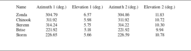


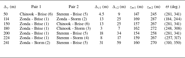


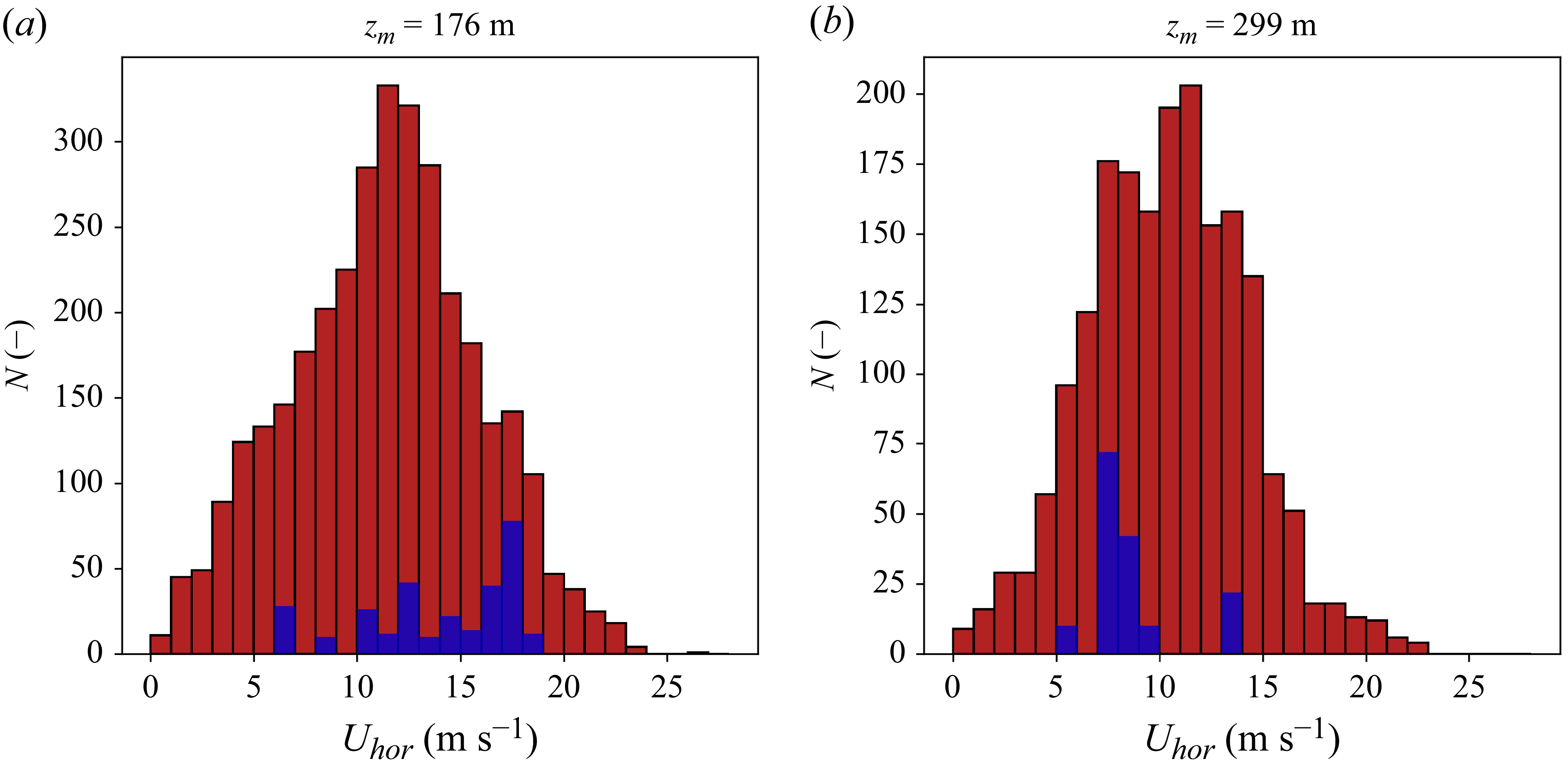


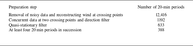
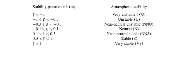


 Open access